an introduction to fluid mechanics - essie - university of …arnoldo/egm5816/classnotes… · ·...
TRANSCRIPT

An Introduction to Fluid Mechanics
Clinton D. Winant1
November 15, 2007
All rights reserved 2007
1Integrative Oceanography Division, Scripps Institution of Oceanography, University of California, San Diego, CA, 92093,E-mail: [email protected], Phone: (858) 534-2067, FAX: (858) 534-0300

Lecture 1
Preliminaries - Fluid Statics
What is a fluid?
The most obvious distinction between a fluid and a solid is theability of the fluid to deform. Very generally, a solidhas a definite shape that changes only a little when external forces are applied. In contrast a fluid element has nopreferred shape, and the application of force usually givesrise to motion.
To be precise we say that fluids cannot support a shearing stress without continuous deformation. Note thatwe are making a distinction between normal and shear stresses. To visualize this, fill a tank of water nearly to thetop, and blow a stream of air over the surface of the water. As soon as the air exerts a stress (this is a shear stress,because it is directed parallel to the free surface, a normalstress would be directed at right angles to the surface)the water begins to move. At the surface the water moves with the stress, but elsewhere in the fluid, the directionand amplitude of the motion varies considerably. The defining feature here is that the motion, or deformation, ofthe fluid continues until the stress is removed. We see that ina fluid, theshearstress is proportional to the time rateof change of deformation, which in turn is related to the velocity field. For a “Newtonian” fluid:
τ = µe where e =dǫ
dt
Note that if rather than a shear stress, we had exerted a normal stress at the surface, by for instance increasingthe pressure so that there was a net force down on the surface,the fluid would have rapidly adjusted to a newequilibrium. That is how a solid reacts to an imposed force. For elastic solids, the strain ( relative deformation) isrelated to the stress (force per unit area) by:
τ = Y ǫ
whereτ is the stress,Y is Young’s modulus, a constant for an elastic solid, andǫ is the strain. Fluids react to normalforces just as solids react to both normal and shear forces, there is some deformation, but no continuous deformation.This definition implies that when we describe the forces exerted by one volume of fluid on a neighbouring volumewe will have to distinguish between normal and shear stresses.
1

H
τundisturbedwater level
disturbedwater level
Figure 1.1: A fluid will undego continuous motion when a shearstressτ is applied
The Continuum approximation
While we understand that at a molecular level matter is made up of discrete particles, we normally experiencematter and in particular fluids as a continuous medium, by which we mean that properties (for instance density) aredistributed continuously, as smooth functions of space andtime. If the scales of the flow considered (say10−4 to107 m) are much greater than molecular scales (say the mean free path between molecules), this is reasonable, andconstitutes the Continuum approximation, adopted throughout this class, and throughout oceangraphy and greatchunks of meteorology. So any propertyθ will be written as
θ = θ(x, t)
the arguments on the right hand side are theindependentvariables of the problem: the positionvector,x, and time,t, which is a scalar quantity.
Diffusive fluxes
We need to allow for important molecular processes to be represented in the continuum description. Diffusion isthe process by which molecules intermingle as a result of their kinetic energy of random motion. Consider twochambers of gas separated by a partition. The molecules of both gases are in constant motion and make numerouscollisions with the partition. If the partition is removed the gases will mix because of the random velocities oftheir molecules. In time a uniform mixture of molecules willbe produced in the container. It is observed thatquite frequently theflux of some property going from one medium to the next is proportional to the gradient of thatproperty. The best known example of this is Fourier’s heat conduction law which staes that if there is a temperature
2

gradient in some medium, then there exists a heat fluxq = −k∇T which is the continuum representation ofinteractions at the molecular level. The constantk is called the conductivity. It varies with different matter, andcan also vary as a function of the independent and the dependent variables. In general the heat flux is a vector thatcarries heat from high temperature regions to low temperature regions, or against the temperature gradient, whichexplains the minus sign. Sometimes this is called a downgradient flux. In many cases, properties such ask aretaken as constants. As a second example, consider a still fluid in a container, in which the salinity varies from somelarger value near the bottom to a smaller value near the surface. Molecular diffusion will drive a flux of salt fromthe bottom to the top of the tank, proportional the vertical gradient of the salt, and characterized by some diffusivitycoefficient. It is very important to understand that the diffusive process affects all properties, including momentum.In this case, because momentum is a vector, for an incompresible fluid, the diffusive law is written as:
σij = µ
(
∂ui∂xj
+∂uj∂xi
)
where the constantµ, the “diffusivity” of momentum, is called theviscosity. This form is only strictly valid forwhat we call “Newtonian” fluids, but all fluids we are concerned with (air, water) qualify. The diffusive flux of ascalar quantity (temperature) is a vector (q). The diffusive flux of a vector (momentum) is atensor, σij . But this isonly a complexity of form. The basic idea for temperature, momentum, or any other property is the same: randommolecular motion causes a kind of stirring at that level thatis accounted for in the continuum approximation bythese diffusive fluxes.
Boundary conditions
The existence of diffusive fluxes has important applications as far as boundary conditions are concerned. If forinstance two media are in contact, say hot iron is pushed intowater, then there will be a flux of heat out of theiron into the water. In other words whatever property fluxes out of one medium has to flux into the neighbouringmedium. In the case of the container of salt water, since saltcan’t diffuse into either the container or the air above,the boundary condition in the water, at the surface or at the bottom, will have to be that the diffusive salt flux iszero, which implies that the salt gradient normal to these boundaries is zero. A related issue has to do with how thevelocity changes at the boundary between a fluid and a solid. Studies have shown that at the molecular level, fluidmolecules enter the solid lattice, for a short while. When they emerge back into the fluid, their average velocity isequal to the average velocity of the solid. In the continuum view this translates into theno-slipboundary conditionthat states that at a solid boundary, the velocity of the fluidparallel to the boundary is the same as the velocity ofthe boundary. Of course the velocity of the fluid normal to theboundary has to be zero relative to the boundary aswell.
3

Fluid Properties
Independent variables
The first point is that there are three kinds of variables. Themost obvious are variables like time or temperatureor density or pressure that need a single number to representthem. These are SCALARS. other variables such asposition or velocity are VECTORS, they require three numbers for their representation. I will use the waves bookconvention of representing a vector (something that has both a length and a direction) by a bold character) For acartesian coordinate system the three numbers are the projections of the vector along each of the axis, so we canwrite
x = ix+ jy + kz
Note that you need to read carefully and distinguish betweenthe boldx which means the whole vector andxwhich represents just the component along thex-axis. So when you read these formulas be attentive. Is it a vectorrelationship or a scalar relationship? Are there tensors? You also need to be aware that there are other coordinatesystems (cylindrical, spherical, etc..) where the components are a little different, see for instance sec 2.4, page32. The essential thing here is that vectors require three values for their specification, because they have a lengthAND an orientation. A lot of times, to keep the algebra simple, we talk about “two dimensional flow” in which weimplicitly assume that everything that happens along the y-axis (or sometimes the z-axis) is zero. In that case thereare only two-values.
x = ix+ kz
In this case the flow is said to be in thex, z plane,v and∂/∂y are everywhere zero.
Scalars
Some properties such as density (ρ) or temperature require a single value for their specification and are calledscalars. Pressure (p) is another important scalar property. Pressure is defined as the force per unit area in thedirectionnormal to the area. In a fluid at rest the pressure is independant of direction.
Vectors
Position (x) and velocity (u) are examples of prperties that require three values for their specification, these arecalled vectors and can be written either as
u = u(x, t)
or, using the indicial notationui = ui(xi, t)
when the index is not repeated, it refers to the collection ofindividual items, thusui means exactly the same thingasu.
4

Tensors
Some variables require 9 values for their specification, These are called tensors. One example is the stress tensor.We write
τij = τij(xi, t)
sincei, j each take on the values 1, 2 and 3,τij means the collection of 9 values. Stress is force per unit are. Bothforce and area have a direction. Consider an x-directed areaelement:
The convention is that the first index (i) refers to the direction of the normal to the surface while the second(j) refers to the direction of the force. Stresses are always reported in a right hand coordinate system in which theoutward directed normal to the surface indicates the positive direction, so:
If the outward normal points in the same direction as the coordinate axis, then the stresses are positive in thedirection of the coordinate and vice-versa.
The sum of the forces acting on a closed surfaceA is then∮
Aτijnida
For a fluid at rest, the shear stresses are zero, and the normalforces are due to pressure, with the result that
τ11 = τ22 = τ33 = −p
where the− sign is required by the sign convention for stress. We will see further on that for a fluid in motion
τ11 + τ22 + τ333
= −p
Hydrostatics
The hydrostatic equation
Consider the force balance on the little volume of water surrounded by a dashed line. On the lower line, atz = z0,say the pressure isp(z0), so the force exerted on the volume is directed up with magnitudep(z0)A. We expect thepressure at the top of the dashed volume is somewhat different from that at the bottom, so we express it as a Taylorseries expansion about the lower level:
p(z = z0 + dz) = p(z0) +
(
∂p
∂z
)
z0
dz + ...
That pressure exerts a downward force on the control volume.Finally gravity exerts a downward forceW =−ρgdzA. The sum of all these forces has to be zero:
p(z0)A−[
p(z0) +
(
∂p
∂z
)
z0
dzA
]
− ρgdzA = 0
5

g
z
dz
p
p+ dzdpdz
Surface area=A
z=z0
z=z +dz0
Figure 1.2: Force balance in a glass of still water
we can divide bydzA, and the termsp(z0) on the right hand side cancel so, the force balance in thex andydirection give∂p/∂x = 0 and∂p/∂y = 0, so p is only a function ofz, and we are left with the hydrostaticequation:
dp
dz= −ρg
The minus sign is due to the fact thatz increase in the opposite direction from gravity. We don’t need partialderivatives because if the fluid is static, the pressure onlydepends onz (along as thez axis is parallel to gravity). Ifand ONLY if the density is constant, then this can be integrated as
p = −ρgz + C
where C is a constant of integration.
Example 1
Consider the problem of an empty glass of weightW in air, that rests upside down near the surface of a large tankof water. We know the constant density of water,ρ, the heightH of the glass, and its diameterD, and we are toldthat the air density is so small it can be ignored, sayρa = 0.
The first thing is to decide where to place the reference for the z-axis. Since the air density is zero, a convenientplace is the water surface, since the pressure there must be zero. Sincep = 0 at z = 0, we see the constantC = 0,so as we descend to the level of the lip of the glass, located atz = −h, the pressure isp = ρgh. It is crucialto realize that because the fluid is not in motion (hydrostatics), there is no pressure difference in either thex or ydirection, so the pressure just under the glass isp = ρgh. Since the density inside the glass is zero, the pressureeverywhereinside the glass isp = ρgh. What force does this exert on the glass? Force is a vector, and so has both
6

z
H
h
Figure 1.3: Upside down glass resting on a pan of water
a direction and a magnitude. Thedirection of the force is given by the direction of the area on which pressure isacting, and the magnitude of the force is given the product ofthe pressure by the area. IfAg = πD2/4 is the areaof the glass, then the pressure in the glass exerts an upward forceFz = ρghAg on the glass. It is important not toforget that the pressure is also pushing against the sidewalls of the glass. At each point on the periphery of the glassthere is a radially outward force. However, since the glass is symmetric, all the radial forces cancel out. What is theforce balance in thez direction? The pressure force is pushing up and the weight ofthe glass is pulling it down, sothe glass will come to equilibrium when
ρghAg = W
This tells us that the depthh = W/(ρgAg). The other way to solve this problem is to invoke Archimedes’principlethat say that there is a buoyant forceFB equal in magnitude to the weight of fluid displaced by the body. In thisproblem, thevolumeof displaced by the fluid is justhAg, soFB = ρghAg . If we equate this to the weight of theglass, we get exactly the same result as above, which is good news, since Archimedes’ principle is EXACTLY thesame thing as what we did above. In other words the reason for the existence ofFB is the fact that by immersingthe glass, the pressure inside is raised in such a way as to produce an upward force.
Example 2
Consider the same water tank as above, but without the water glass. The tank is rectangular in section, with lengthL and widthW into the paper, so that the bottom area of the tank isAT = LW . The depth of the water from thesurface to the bottom isD, We want to know what force the water exerts on the sides and bottom of the tank. Theforce on the bottom is simply the product of the pressure at the bottomρgD time the bottom area:FB = −ρgDAT .The minus sign is needed because the force points down, in theopposite direction from thez-axis. SinceDAT isthe volume of the water in the tank, we see that the downward force due to pressure is just equal to the weight of the
7

x
z
dFx
D
zR
Fx
Figure 1.4: Detail of tank sidewall
water. Now what about the forces on the vertical sides? The force certainly points away from the tank, the wateris pushing out against the walls, but how large is that force?This is a little more difficult, because the pressurechanges along the sidewall. It is zero at the surface of the water and increases toρgD at the bottom. If we thinkabout the side as being made up of a lot of very small elements,that have width into the paperW and heightdz,then the force acting on any such element isdFx = pWdz, where the subscriptx is meant to remind us that this isa force in thex direction. Since pressure is zero at the surface, we know that p = −ρgz, sodFx = −ρgWzdz. Toget the total surface we integrate from the bottomz = −D to the surface:
Fx = −∫ 0
−DρgWzdz = −ρgW
(
z2
2
)0
−D
= ρgWD2
2
This makes sense, if you think that the average pressure acting on the sidewall isρgD/2. and the area isDW , thenthe force is the same as above. Of course there is a force exactly equal to this on the opposite sidewall, so thenetforce is zero, however all these forces are working to stretch the tank outward. Often the question is asked of wherethe resultantforce acts. The magnitude of the resultant force is as given above forFx, the location of the resultantforce is such that themomentof all the elementaldFx forces add up to zero:
FxzR = −∫ 0
−DρgWz2dz = −ρgW D3
3
8
D
L
H
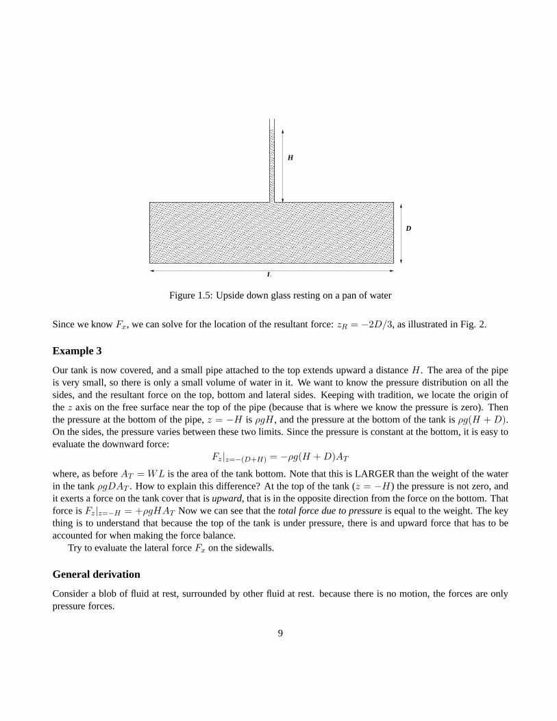
Figure 1.5: Upside down glass resting on a pan of water
Since we knowFx, we can solve for the location of the resultant force:zR = −2D/3, as illustrated in Fig. 2.
Example 3
Our tank is now covered, and a small pipe attached to the top extends upward a distanceH. The area of the pipeis very small, so there is only a small volume of water in it. Wewant to know the pressure distribution on all thesides, and the resultant force on the top, bottom and lateralsides. Keeping with tradition, we locate the origin ofthez axis on the free surface near the top of the pipe (because thatis where we know the pressure is zero). Thenthe pressure at the bottom of the pipe,z = −H is ρgH, and the pressure at the bottom of the tank isρg(H +D).On the sides, the pressure varies between these two limits. Since the pressure is constant at the bottom, it is easy toevaluate the downward force:
Fz |z=−(D+H) = −ρg(H +D)AT
where, as beforeAT = WL is the area of the tank bottom. Note that this is LARGER than the weight of the waterin the tankρgDAT . How to explain this difference? At the top of the tank (z = −H) the pressure is not zero, andit exerts a force on the tank cover that isupward, that is in the opposite direction from the force on the bottom. Thatforce isFz|z=−H = +ρgHAT Now we can see that thetotal force due to pressureis equal to the weight. The keything is to understand that because the top of the tank is under pressure, there is and upward force that has to beaccounted for when making the force balance.
Try to evaluate the lateral forceFx on the sidewalls.
General derivation
Consider a blob of fluid at rest, surrounded by other fluid at rest. because there is no motion, the forces are onlypressure forces.
9

The total body force acting on the fluid in volumeV is∫
ρg dV
The total contact force exerted by the surrounding fluid at the surfaceA boundingV is
−∫
pn dA
wheren is the unit vector pointing outward fromA. The minus sign is needed to represent the forces acting onV
from the surrounding matter.Then
−∫
pn dA = −
∫
∇p dV
Since the sum of the forces must be zero∫
(ρg −∇p)dV = 0
But the integral has to be zero no matter what the volume of integration is. The only way this is possible is for theintegrand to be everywhere zero:
ρg= ∇p
We always choose a coordinate system in which thez axis is vertical and pointing up, in other wordsg= −kg,
wherek is the unit vector in thez direction andg is the magnitude of gravity (9.81 ms−2). In this case, the vectorequation above has the following three components:
∂p
∂x= 0
∂p
∂y= 0
∂p
∂z= −ρg
The last equation is called the hydrostatic equation. The minus sign comes from the fact that positivez is in the
opposite direction fromg . In the special case when the density is not a function ofz, it can be integrated to give:
p = −ρgz + pa
10

wherepa is a constant of integration: to knowp, you need to know what the pressure is at some level. If, for instancep = pa at the surface of the ocean, wherez = 0, the equation forp says that pressure increases asz becomes morenegative, that is with increasing depth.
It is important to understand that theforce due to this pressure is avector. If the pressure is constant over asmall area element, then the force is
F= pA
n
wheren is the direction of thenormal to the surface. So the direction of the force is entirely determined by the
orientation of the surface, whereas the manitude is detrmined by the product of the pressure times the area.As an example consider a rectangular tank of heightH lengthL and widthW , filled with still fluid and open at
the top.
z g
HF
FF
z
xx
x
If the pressure at the surface (z = 0) is the atmospheric pressurepa, then the pressure just above the bottom ofthe tank isρgH + pa (because the tank bottom is located atz = −H). The force due to that pressure on the bottomsurface is directed down (in the−z direction):
Fz = (pa + ρgH)LW
It is important to understand that the pressure that gives rise toFz also creates a forces on the vertical sides of thetank. The direction of that force is normal to the sidewal, orin thex direction. The magnitude is more complicatebecause the pressure changes along the vertical wall: near the surface (z = 0) it is close topa, and near the bottom,it is is pa + ρgH. To get the magnitude of this force we have ti intgrate the variable pressure. For the right handsidewall
Fx = W
∫ 0
−Hpdz = W
∫ 0
−H(pa − ρgz)dz = paHW + ρg
H2
2
On the left sidewall the pressure exerts a force in thex-direction of equal magnitude but the direction is opposite,so thex-directed forces cancel out.
11

Lecture 2
Flow Field Specification
Eulerian & Lagrangian descriptions
How will we describe the flowfield? Two possibilities come to mind. The first is to describe what hapens at somefixed point−→x and at timet. Thus for velocity we would say
−→u = −→u (−→x , t)
This is what is called the Eulerian description, a simple wayto think about this is to think of making obserbationsat some number of fixed positions, as a function of time, or to think of the output of a numerical simulation of theflow, where the grid is fixed in space.
A second possibility is to describe the history of each property of each indivudual parcel of mass. So forvelocity,
−→v = −→v (−→x0, t)
where−→x0 is the position of a parcel of fluid at some initial timet0. This is called the Lagrangian description,and corresponds more or less to what we do when we track drifters in the ocean, or balloons in the atmosphere.
For almost all the work in this class, we will stick with the Eulerian description.
Specifying the velocity field and trajectories
Just as we map out a scalar variable by plotting the locus of constant values of the variable, a contour plot, thereare three ways to illustrate a flow field. If the flow is steady, that is it does not vary in time (∂/∂t ≡ 0), all threedescriptions are the same.
12

Streamlines
Streamlines are defined to be at any time parallel to the velocity vector. The idea of a snapshot is inherent to theconcept of streamlines, that is for an unsteady flow streamlines patterns change as a function of time. In a Cartesiancoordinate, and for a two dimensional flow (a flow for which there is no change in the third dimension) the slope ofa streamline is simply given by
dy
dx=v
u
For a three-dimensional flow, this can be extended to
dx
u=dy
v=dz
w
Note that since fluid cannot flow across a boundary, they must be streamlines.
Pathlines
A pathline is the trajectory of one identified mass parcel. Imagine dying a prticular element of fluid, them thepathline is the line drawn betwen all the positions that the marked parcel has moved through. Pathlines extend withtime, and correspond to the trajectories of neutrally buoyant drifters, or ballons. In two dimensions, the equationfor a pathline can be derived by integrating
x = x0 +
∫
t0udt
y = y0 +
∫
t0vdt
wherex0, y0 are the location of the identified parcel att0.
Streaklines
A third way of describing a flow would be to indroduce dye or smoke into the flow at a given positionx0, y0, thentaking pictures at some timet of the locus of all the marked parcel, or the dye or smoke line.
The Streamfunction
In two-dimensional or axisymmetric flow it is convenient to define a streamfunctionψ such that
u =∂ψ
∂y
13

v = −∂ψ∂x
Consider a point A on one streamline and a point B on another streamline. What is the flux of massρQ of fluidacross the line AB? If AB is parallel toy, thenQ = udy. In general, , if the surface AB is defined by (dx1, dx2),thenn = idy − jdx, so thatu · n = udy − vdx. ThenQ = udy − vdx, or
Q =∂ψ
∂ydy +
∂ψ
∂xdx = dψ
If A and B are on the same streamline, thenQ ≡ 0, soψ must be a constant along a streamline. Another way to seethis is to remember the definition of a streamline in two dimensions:
dx
u=dy
v
If we introduce the streamfunction:
dx∂ψ∂y
=dy
−∂ψ∂x
We can manipulate this to give
∂ψ
∂xdx+
∂ψ
∂ydy = dψ = 0
which also shows thatψ is constant along a streamline (but doesnt make the point that the transport betweenstremlines is given by the difference in the streamfunction).
Differentiation following a fluid parcel
If we adopt the Eulerian description, we are going to have to express the rate of changes of properties following amaterial parcel, ie we will want to ask how much the temperature of a given blob of fluid changes with time, whichis different from asking how much the temperature changes atsome point−→x . For an arbitrary propertyQ, the chainrule tells us:
dQ
dt=∂Q
∂t+∂Q
∂x
dx
dt+∂Q
∂y
dy
dt+∂Q
∂z
dz
dt
but for a fluid parcel,u = dx/dt, etc..., so
dQ
dt=∂Q
∂t+ u
∂Q
∂x+ v
∂Q
∂y+ w
∂Q
∂z
14

in shorthand:
dQ
dt=∂Q
∂t+ u.∇Q =
DQ
Dt
where the capital D is used as a way to remember we are talking about the dericative following a fluid parcel,also know as the total derivative. This consists of two parts: one is simple the local rate of change with time, andthe other,u.∇Q, is the rate of change due to transport between two positionswhereQis different. This later part isthe “advective” change. It is important to note that even in asteady flow, the total rate of change is not necessarilyzero.
15

Lecture 3
Global Conservation Equations
Advective fluxes
The advective flux of any property (scalar, vector,...) is the amount of that property that crosses a surface per unittime. Think for instance of the number of cars going through atoll both per unit time, that would be the flux of carsacross the width of the freeway. When we talk about a flux, we need to have a surface in mind. For some (intensive)propertyQ (for mass, this is the densityρ) the flux is equal toQ times the velocity normal to the surface consideredtimes the surface area. For an elemental areasdA:
F = Qu · ndA
wheredA represents the magnitude of the area element andn represents the normal direction to the surface element.The mass flux is thusρu · ndA. The total mass flux out of a volume bound by the closed surfaceA is thus:
∫
Aρu · ndA
If the variable of concern is a vector (momentum for instance), then the flux is also a vector:
F = (ρu)u · ndA
Mass Conservation
Statement:
In the absence of sources or sinks of mass, the change of mass within a fixed volume (the control volume) is equalto the difference between the fluid flowing into and out from the volume. Consider an arbitrary, potato shapedfixedCV, The total amount of fluid in the volume is
∫
ρdv, and the total flux into the CV is− ∫ ρu.nda∂
∂t
∫
ρdv +
∫
ρu.nda = 0
16

Note that if the density is constant and the volume is fixed, then the sum of the fluxes must be zero. This means thatthevolumeis conserved.
Examples
One dimensional flow of an incompressible fluid
Consider a pipe or duct of varying diameter.
ρ1A1V1 = ρ2A2V2
If the density is constant this becomesV1A1 = V2A2 = Q
Water fawcet
Traffic flow: variable density
Consider a section of a road as a control volume. There is a traffic signal at the downstream end through which themaximum flow rate is 1 car per second. On the upstream end cars enter the control volume at a rate greater than 1car per second?
For steady flow∂ρ/∂t = 0, notDρ/Dt = 0, so∇.−→ρu = 0. This means that the flux of cars through any twosections has to be the same, but in this casebothu andρ can change, and there is a very definite maximum toρ. Soif youre caught in bumper to bumper, and all of a sudden another lane opens what happens? Not obvious that yougo twice as fast, because car separation tends to increase, so density decreases. What about the reverse situation,two lanes become one? If the traffic is choked before the constriction, then your speed will increase when you getto the single lane!
Tidal flow in an estuary: variable volume
Mass inside the estuaryρ (H + η) (L− x)WFlux into estuary from the ocean:ρu (H + η)WSolve foru
u (x) =L− x
H + η
∂η
∂t
order of magintude estimates,
Momentum Theorem
Statement
The time rate of change of momentum contained within afixedcontrol volume plus the net flux of momentum outof the surfaces is equal to the sum of all forces acting on the volume.
17

Mean water depth
L
u(x,t)H
W
x
η( t)
∂M
∂t+
∮
Aρuu.nda = F
whereM =
∫
Vρudv
andF = Σ(body forces+ surface forces) = g
∫
Vρdv +
∮
Aτijnjda
Becausen is defined to be positive outward, the surface integral on theleft hand side of the equation represents themomentum fluxout of the control volume.
Body forces are due to a force field such as gravity. If, as in the case of gravity, this field is conservative, thefield cam be written as the gradient of a potential:
g = −∇(gz) = −kg
where we have assumed that thez-axis points up.Surface forces are those exerted by neighboring fluid elements at the boundaries of the element being consid-
ered. In general this force is at some arbitry angle to the surface. The force per unit area (stress) can be decomposedinto components normal to the surface (normal stress) and parallel to the surface (shear stress).
18

Examples
One dimensional flow of an incompressible fluid
Return to the variable area straight pipe, the flow is steady so the local change in time is zero. For the momentumtheorem in thex-direction, the net flux of momentum out
ρV 22 A2 − ρV 2
1 A1 = ρQ(V2 − V1)
Ignoring friction, the only forces acting in thex-direction are due to pressure:
p1A1 − p2A2
If we know conditions at the entrance, and the area at the exit, conserving mass givesV2, and the momentumtheorem gives usp2. Consider the length of the pipe to be very small, equal toδx, and the area to change by only asmall amount, then the momentum theorem can be written
ρQδV = −Aδp
Divide by the volume, and take the limit asδx becomes small:
ρVdV
dx= −dp
dx
Integrating along x then givesρ
2V 2 + p = constant
which we will see later is Bernouilli’s equation.
A bent pipe
Think about a constant diameter pipe that is bent by some angle θ along its length. What force does the pipe exerton the fluid to cause the stream to bend? The densityρ, velocityV and cross-sectionA are constant. The flow issteady, and we consider only thex component, so the momentum theorem reduces to
∮
Aρuu.nda = F
whereD is the force exerted by the body on the fluid. We look at the momentu theorem inx andy directionsseparately:
Fx = ρV V cos θA− ρV 2A = ρV 2A(cos θ − 1)
and, in they-direction:Fy = ρV 2 sin θA
19

Drag on a body immersed in a flow
It is useful to consider first the mass concervation principle for the control volume drawn above:
−2ρU0B + 2ρ
∫ L
−Lwdx+ ρ
∫ b
−bu(z)dz = 0
Then evaluate the flux ofx momentum into the control volume:
−2ρU20B + 2ρ
∫ L
−Luwdx+ ρ
∫ b
−bu2(z)dz
Now takeB to be large enough that u in the first integral can be taken to beU0, and set the sum of the fluxes equalto the force:
−2ρU20B + 2ρU0
∫ L
−Lwdx+ ρ
∫ b
−bu2(z)dz = D
Use the conservation of mass result to evaluate the first integral:
−2ρU20B + ρU0
(
2U0B −∫ b
−bu(z)dz
)
+ ρ
∫ b
−bu2(z)dz = D
or:
D = ρ
∫ b
−bu(u− U0)dz
The sign is negative because the force exerted by the body is in the opposite direction from the flow.WHat about thez-direction? w
Tidal flow in an estuary
Mx = ρW
∫
(H + η) udx
20

Flux(x = 0) = ρ (H + η)Wu2
PressureForce(x = 0) = W
∫ H+η
pdz = ρWg(H + η)2
2
PressureForce(x = L) = W
∫ H+η
pdz = ρWg(H + η)2
2
Bottomstress = (2H +W )
∫
τdx
INCLUDE SUMMARY FIGURE
21

Lecture 4
Local Conservation Equations
Mass Conservation
In the last lecture we concludes that for any volume surrounded by a closed areaA
∂
∂t
∫
ρdv +
∫
ρu.nda = 0
If we apply this to a small fixed volume with sidesδx, deltay anddeltaz, the flux term can be written as
[ρu+∂(ρu)
∂xδx]δyδz − [ρu]δyδz + [ρv +
∂(ρv)
∂yδy]δxδz − [ρv]δxδz + [ρw+
∂(ρw)
∂zδz]δxδy − [ρw]δxδy
This proves the divergence theorem, relating the integral over a volume to the integral over the closed surfacesurrounding the volume:
∫
∇ · (ρu)dv =
∮
ρu.nda
Other forms of the Divergence theorem are:∫
∇θdv =
∮
θnda
whereθ represents any scalar variable, and
∫
∂τij∂xj
dv =
∮
τijnjda
for any tensorτij . Thus∫(
∂ρ
∂t+ ∇ · ρu
)
dv = 0
22

This has to be true for any volume, and so the integrand has to be zero:
∂ρ
∂t+ ∇ · ρu = 0
This can be written as:∂ρ
∂t+ u · ∇ρ+ ρ∇ · u = 0
or, with the definition ofD/Dt;Dρ
Dt+ ρ∇ · u = 0
This is the local version of the full continuity equation
The special case of incompressible flow
If the density of a fluid parcel is constant (note this is less restrictive than to say the density of the fluid is constant),thenDρ/Dt = 0, an we get the special result that∇ · u = 0. But this eliminates compressibility and soundwaves, and the ability to understand how a fluid adjusts to changes in pressure. It forces us to think that fluid reactsinstantaneously to changes in pressure. In this case the local conservation of mass becomes:
∇ · u =∂u
∂x+∂v
∂y+∂w
∂z= 0
whereu, v, w are the components ofu. What is the equivalent form for a polar , cylindrical coordinate system?
Momentum
Now the starting point, from the last lecture, is:
∫
∂ρui∂t
dv +
∮
ρuiujnjda =
∫
ρgidv +
∮
τijnjda
Use the Divergence integral for tensors to rewrite the area integrals:
∫
∂ρui∂t
+∂(ρuiuj)
∂xj− ρgi +
∂τij∂xj
dv = 0
where we have used the fact that the volume integral must be zero for any arbitrary volume of integration, so thatthe integrand must be zero. Expanding the derivatives of thefirst two terms:
ui[∂ρ
∂t+∂(ρuj)
∂xj] + ρ[
∂ui∂t
+∂(uiuj)
∂xj] = ρgi +
∂τij∂xj
23

But the first term on the left is zero by continuity, so the momentum equaton simplifies to:
ρ[∂ui∂t
+∂(uiuj)
∂xj] = ρgi +
∂τij∂xj
Note that this is valid for any deformable medium, solid, liquid or fluid. Note also that this is a vector equation(equivalent to 3 scalar equations) with a total of 12 dependant variables, even ifρ is assumed to be constant.
ρDu
Dt= ρg +
∂τij∂xj
valid for anycontinuous medium (fluid or solid).
The relation between stress and rate of strain
With this equation and Mass concervation we have four equations in thirteen unknowns! Need a relation betweenthe flow field and the stress tensor. SInce for a fluid at rest only the pressure exists, we can write:
τij = −pδij + σij
σij is called the “deviatoric” part of the stress tensor. It parameterizes the diffusive flux of momentum. For anincompressibleNewtonianfluid, we write
σij = µ
(
∂ui∂xj
+∂uj∂xi
)
The minus sign in front of the pressure is needed for consistency with the sign convention for tensors.
More detail
The most general form forσij is
σij = 2µ
(
eij −2
3eiiδij
)
whereδij is the kronecker delta, andeii = ∂ui/∂xi = 0 whenDρ/Dt = 0.For a term likeτ12:
τ12 = µ
(
∂u1
∂x2+∂u2
∂x1
)
and, for incompressible flow,
τ11 = −p+ 2µ∂u1
∂x1
24

This is what we call a “Newtonian” fluid, and can be taken as thedefinition of bothp and the viscosityµ.How to interpret this? For Couette flowτ12 = τ12 = µ∂u1/∂x2, this is analogous to the Fourier heat conduction
law: q = k∂T/∂x. Back to the momentum equation, for incompressible flow:
∂τij∂xj
= − ∂p
∂xi+ 2µ
∂eij∂xj
2µ∂eij∂xj
= µ
(
∂2ui∂xj∂xj
+∂2uj∂xi∂xj
)
but the last term in the parenthesis is zero because we can write it as:
∂
∂xi
∂uj∂xj
and for incompressible flow
∂uj∂xj
= 0
and,
∂τij∂xj
= −∇p+ µ∇2u
Putting it all together, the momentum eqaution for an incompressible fluid is:
ρDu
Dt= −∇p+ ρg + µ∇2u
Strain rates
We think of strain, or deformation, as consisting of two parts, linear strain, or elongation, and shear strain.
Linear Strain
Consider an element of mass that is pulled out from some initial lengthAB to a new lengthA′B′. we define thestrain to be the relative change in length, or:
ǫ =A′B′ −AB
AB
if the velocity of pointA is u, and the velocity of pointB is u+ (∂u/∂x) δx, andδx is the lengthAB,
25

A B A’ B’
A
B
A’
B’
Figure 4.1: Strain and deformation
ǫ =AB +BB′ −AA′ −AB
δx=
(
u+ ∂u∂xδx− u
)
δt
δx
and the strain rate,exx = ǫ/δt, is exx = ∂u/∂xThis reasoning can be extended to a volume and gives the volumetric strain rate:
eii =1
δv
d (δv)
dt=∂u
∂x+∂v
∂y+∂w
∂z=∂ui∂xi
For an incompressible fluid, the volumetric strain rate is zero.
Shear Strain
In a two dimensional plane, the deformation is defined in terms of the two anglesφ1 andφ2.
φ2 =B′B −A′A
δy
the velocity of pointA is u, and the velocity of pointB is u+ (∂u/∂y) δy, andδy is the lengthAB,
φ2 = −
[(
u+ ∂u∂y δy
)
− u]
δt
δy
where the minus sign comes about because we define positive rotations to be CCW. The shear deformation rateis thendφ2/dt = −∂u/∂y, and similarlydφ1/dt = ∂v/∂x. The rate of shear strain is then:
dφ
dt=dφ1
dt− dφ2
dt=∂v
∂x+∂u
∂y
26

And the deformation can be described by the strain rate tensor eij :
eij =1
2
(
∂ui∂xj
+∂uj∂xi
)
But since the linear strain rate iseii = ∂ui/∂xi, the expression above describes all cases: the diagonal termssare the linear strain rates, and the off-diagonal terms are half the shear starin rates.
Rotation rate
The derivation of the shear deformation can be used to define the rotation of a fluid parcel: for instance the rotationalong the z-axis is given by
rk =d
dt(φ1 + φ2) =
1
2
(
∂v
∂x− ∂u
∂y
)
wherer is a vector.More usefully, we define the vortivity vector, as twice the rotation rate:
1 =
(
∂w
∂y− ∂v
∂z
)
2 =
(
∂u
∂z− ∂w
∂x
)
3 =
(
∂v
∂x− ∂u
∂y
)
or: = ∇× u, the vorticity is the curl of the velocity.
27

Lecture 5
Boundary Conditions
A flow system is only fully specified once boundary conditionshave been established. The boundary conditionscharacterize a flow system and make it distinct from other flows (the equations of motion in priciple apply to allflow systems). We often talk about two different kinds of boundary conditions: kinematic and dynamic.
Kinematic Boundary Conditions
Unless physical tearing occurs at a boundary, it must remaina material surface for both bounding media. The mostobvious implication is that at any boundary the normal component of velocity must be constant; were this not truethe boundary would split apart, an obviously unacceptable result.
To express this in math:u.n = ub.n
whereu is the fluid velocity,ub is the velocity of the boundary and .n is the unit vector normal to the body.A somewhat less obvious example of a kinematic boundary condition is that the velocity component parallel
to the body must be continuous acroos the boundary. This is the Stokesno slip boundary condition that can beexplained on a molecular basis. At the contact point betweenmedia, there are molecular exchanges that wouldimmediately wipe out any discontinuity, including in velocity, across the boundary. Since the basis for the noslip condition lies in molecular processes, it must not be applied when the viscosity of a fluid is taken to be zero.Mathematically:
u|boundary = ub
Dynamic Boundary Conditions
If some quantity such as heat or momentum has a flux out of one medium at a boundary, that same flux must enterthe other medium. In terms of the momentum flux this means thatthe stress tensors on either side of a medium must
28

be equal. An obvious example is that the pressure remains unchanged across a boundary, although this statementmust be modified if there is surface tension present, that is if deflections of the surface give rise to a force along thesurface.
In the same way that the no slip boundary condition must be relaxed, the shear stress cannot be assumed constantacross the boundary in an inviscid fluid.
Solid Boundaries and Free Surfaces
It is practically very important to distinguish between solid boundaries, where the shape of the surface is knowna priori, and deformable boundaries as exist for instance between two fluid media (say water and air), where bothkinematic and dynamic boundary conditions are required. The latter class of problems, known asfree surfaceproblemsinvolve the further complexity that the location of the boundary is not known so must be found as partof the solution of the problem. This makes the problemnon-linear just as when dependant variables appear to agreater power than one in the equations so superposition of solutions will not work. One common way around thisproblem is to assume that the displacement of the free surface is relatively small, and apply the boundary conditionat themeanlocation of the free surface. This is one example of a perturbation solution.
Free surface: Open channel flow
µd2u
dz2=dp
dx
u = 0 at z = 0
µdu
dz= 0 at z = h
u = − 1
2µ
dp
dxz(2h− z)
29

Lecture 6
Dynamic Similarity
Similarity Parameters
The equations of motion are:∂u
∂x+∂v
∂y+∂w
∂z= 0
∂u
∂t+ (u · ∇)u + fk× u = −∇p
ρ+ g + ν∇2u
The units of viscosity arePa s, orNm−2s. because the viscosity often appears divided by the density, the parameterν = µ/ρ is the kinematic viscosity is often used. It has dimensionsm2s−1
Define new non-dimensional variables (starred) in terms ofappropriatereference quantities:
t = t∗t0, (x, y, z) = (x∗, y∗, z∗)L0, ∇ = ∇∗/L0,
and(u, v,w) = (u∗, v∗, w∗)U0, p = p∗p0,
The central idea here is that the non-dimensional variablesare of order 1, that is they vary between -1 and +1, ratherthat -100 and +100. Think for instance of a boat of lengthL sailing at velocityU0 and riding on waves whose periodis t0.
With these new variables the equations of motion become:
∂u∗
∂x∗+∂v∗
∂y∗+∂w∗
∂z∗= 0
The continuity equation remains the same as before introducing the non-dimensional parameters. For the momen-tum equation
U0
t0
∂u∗
∂t∗+U2
0
L0(u∗ · ∇∗)u∗ + U0fk× u∗ = − p0
ρL0∇∗p∗ + g +
νU0
L20
∇2u∗
30
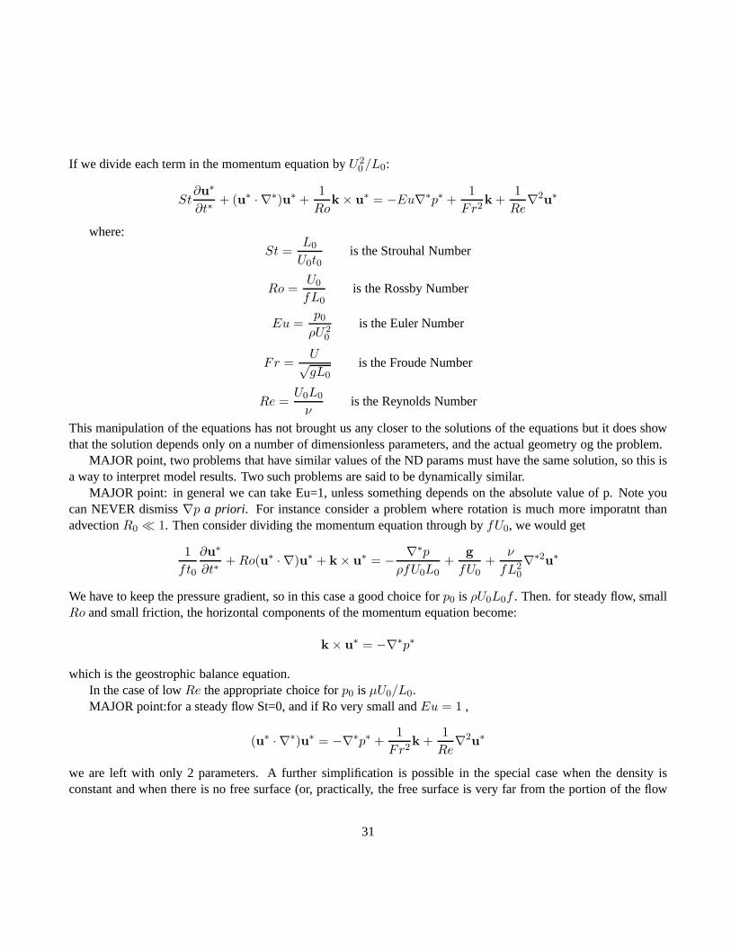
If we divide each term in the momentum equation byU20 /L0:
St∂u∗
∂t∗+ (u∗ · ∇∗)u∗ +
1
Rok × u∗ = −Eu∇∗p∗ +
1
Fr2k +
1
Re∇2u∗
where:
St =L0
U0t0is the Strouhal Number
Ro =U0
fL0is the Rossby Number
Eu =p0
ρU20
is the Euler Number
Fr =U√gL0
is the Froude Number
Re =U0L0
νis the Reynolds Number
This manipulation of the equations has not brought us any closer to the solutions of the equations but it does showthat the solution depends only on a number of dimensionless parameters, and the actual geometry og the problem.
MAJOR point, two problems that have similar values of the ND params must have the same solution, so this isa way to interpret model results. Two such problems are said to be dynamically similar.
MAJOR point: in general we can take Eu=1, unless something depends on the absolute value of p. Note youcan NEVER dismiss∇p a priori. For instance consider a problem where rotation is much moreimporatnt thanadvectionR0 ≪ 1. Then consider dividing the momentum equation through byfU0, we would get
1
ft0
∂u∗
∂t∗+Ro(u∗ · ∇)u∗ + k× u∗ = − ∇∗p
ρfU0L0+
g
fU0+
ν
fL20
∇∗2u∗
We have to keep the pressure gradient, so in this case a good choice forp0 is ρU0L0f . Then. for steady flow, smallRo and small friction, the horizontal components of the momentum equation become:
k× u∗ = −∇∗p∗
which is the geostrophic balance equation.In the case of lowRe the appropriate choice forp0 is µU0/L0.MAJOR point:for a steady flow St=0, and if Ro very small andEu = 1 ,
(u∗ · ∇∗)u∗ = −∇∗p∗ +1
Fr2k +
1
Re∇2u∗
we are left with only 2 parameters. A further simplification is possible in the special case when the density isconstant and when there is no free surface (or, practically,the free surface is very far from the portion of the flow
31

field we are interested in). For example the flow in a duct or...Define thenon-hydrostatic pressurep′ = p + ρgz,then note that
∇p′ = ∇p− ρg
For steady, non-rotating flow, the non-dimensional momentum equation then simply becomes
(u∗ · ∇∗)u∗ = −∇∗p′∗ +1
Re∇2u∗
So the solution isonly a function of the geometry and the Reynolds number.
Typical magnitudes
0.01ms−1 < U < 1ms−1 10−4m < L < 105m
for water:ρ ≈ 103Kgm−3 ν =
µ
ρ≈ 10−6m2s−1
at mid-latitudes,f ≈ 10−4s−1 Range of Reynolds numbers:
1 < Re < 1011
Range of Rossby numbers10−3 < Ro < 108
Examples
Pipe friction
Sabersky page 187
Flow over a body: the drag coefficient
Sabersky page 202
Flow over a body: the lift coefficient
Sabersky page 204
Drag on a boat
Sabersky page 208
32

Lecture 7
Viscous Flows:Re ≪ 1
The full momentum and continuity equations are:There exists a special class of flows, called straight flows, for which the equations of motion take on a reasonably
simple form. The idea is to look at a flow along a single component of the coordinate system, sayu = iu. In thiscase, the conservation of mass guarantees that∂u/∂x = 0. Then it is simple to show that the advective terms in themomentum equation,(u · ∇)u ≡ 0. In cartesian coordinates, the three components of the momentum equation arethen:
∂u
∂t= −1
ρ
∂p
∂x+ ν
(
∂2u
∂y2+∂2u
∂z2
)
0 =∂p
∂y
0 = −1
ρ
∂p
∂z+ g
where it is assumed that the motion is in the horizontal plane, and that thez axis is positive upward. If the flow istwo-dimensional, that is∂/∂y ≡ 0 and the flow is steady,∂/∂t ≡ 0, thex component of the momentum equationreduces to:
0 = −dpdx
+ µd2u
dz2
As it turns out this is also the limit of the N-S equations whenthe Reynolds number is small, so the flowsdescribed here are solutions to viscous flows, even if they are not really straight. In that case the∂2u/∂x2 may needto be retained.
33
Steady flow
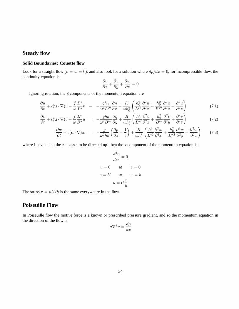
Solid Boundaries: Couette flow
Look for a straight flow (v = w = 0), and also look for a solution wheredp/dx = 0, for incompressible flow, thecontinuity equation is:
∂u
∂x+∂v
∂y+∂w
∂z= 0
Ignoring rotation, the 3 components of the momentum equation are
∂u
∂t+ ǫ(u · ∇)u− f
ω
B∗
L∗v = − gh0
ω2L∗2
∂η
∂x+
K
ωh20
(
h20
L∗2
∂2u
∂2x+
h20
B∗2
∂2u
∂2y+∂2u
∂2z
)
(7.1)
∂v
∂t+ ǫ(u · ∇)v +
f
ω
L∗
B∗u = − gh0
ω2B∗2
∂η
∂y+
K
ωh20
(
h20
L∗2
∂2v
∂2x+
h20
B∗2
∂2v
∂2y+∂2v
∂2z
)
(7.2)
∂w
∂t+ ǫ(u · ∇)w = − g
ω2h0
(
∂p
∂z− 1
ǫ
)
+K
ωh20
(
h20
L∗2
∂2w
∂2x+
h20
B∗2
∂2w
∂2y+∂2w
∂2z
)
(7.3)
where I have taken thez − axis to be directed up. then the x component of the momentum equation is:
d2u
dz2= 0
u = 0 at z = 0
u = U at z = h
u = Uz
h
The stressτ = µU/h is the same everywhere in the flow.
Poiseuille Flow
In Poiseuille flow the motive force is a known or prescribed pressure gradient, and so the momentum equation inthe direction of the flow is:
µ∇2u =dp
dx
34

Plane (two dimensional)
In plane (two-dimensional flow), we take the x axis parallel to the bounding plates, z=0 on the lower plate and theupper plate is at z=h. In this cartesian coordinate system, so long as the flow does not depend ony, the momentumequation is:
µd2u
dz2=dp
dx
Integrating the momentum equation gives:
u =1
µ
∂p
∂x
z2
2+Az +B
The boundary conditions are:u = 0 at z = 0, h
and the solution to the momentum equation is:
u =1
2µ
∂p
∂x(z2 − h2)
It is impotant to remember thatz ≤ h so thatu anddp/dx are of opposite sign. We can say that the flow isdowngradient.
Consider the force balance on a small square element of fluid:on thex sides, the pressure forces combide togive a force−dp/dx, whereas on thez faces the forces combine to givedτ/dz, and the sum of those forces is zero.
Combined Couette and Poiseuille Flow
Because the momentum eqaution for straight flows is linear, solutions can be added linearly, so the flow driven bya pressure gradient between two plates, one of which is fixed while the other moves at velocity U is given by:
u = Uz
h+
1
2µ
∂p
∂x(z2 − h2)
Flow down a plane
Assume the plane makes an angleθ with the horizontal, then thex-component ofgi is g sin θ and thex-componentof the momentum equation is:
0 = g sin θ + νd2u
dz2
with boundary conditions thatu = 0 atz = 0 andτ = du/dx = 0 at the surface,z = H. rewrite as:
d2u
dz2= −g sin θ
ν
35

Integrate the momentum equation twice alongz:
u = − g
2νsin θz2 +Az +B
The boundary condition atz = 0 forcesB = 0, while the boundary condition atZ = H gives:
B =g
νsin θH
so the overall solution is:u =
ρg
2µsin θ(2H − z)z
36

Lecture 8
Unsteady viscous flow
In the previous lecture, the effects of viscosity extended throughout the flowfield, this is what is called fully devel-oped flow. Now we look at time-dependent viscous flows. The major motivation for this, apart from seeing someuseful techniques for solving the heat equation, is that viscous effects are confined to within some finite area nearthe boundary, what is called a boundary layer. We will see later that for viscous flows at high Reynolds numberviscous effects are also confined to a boundary layer near thebody, except when the flow is separated. In manyunsteady viscous flows at low Reynolds number, the subject ofthis lecture, the boundary layer thickness (δ) growsas a function of time, but in periodic flows it remains constant.
For two-dimesional (x, y-plane) straight flow, the component of the momentum in the direction of the flow is:
ρ∂u
∂t= −dp
dx+ µ
∂2u
dy2
When (if) the pressure gradient is zero, this becomes the heat equation, a parabolic linear partial differential equationthat requires one initial condition and two boundary conditions.
Impulsively Started Plate
Consider a plate that is at rest, and immersed in a fluid also atrest. At some initial time the plate is impusivelyaccelerated so that it has velocity U from then on, while the velocity of the fluid far away from the plate remainszero. Consider the case when the pressure gradient is zero, the equation of motion and boundary conditions are:
∂u
∂t= ν
∂2u
∂y2
The boundary conditions fort > 0 are:
u = U at y = 0 u = 0 as y → ∞
and the initial condition isu(x, y, t = 0) = 0. Note that in all there are three conditions.
37

The governing equation is the heat equation, that can be solved by separation of variables, but in this particularcase there is a more elegant solution. Looking at the combination of independant variable in the original equa-tion suggests a new independant variable that is a function of y/
√νt could be useful. This is called asimilarity
transformation. Experience suggests trying
η =y
2√νt
Note the denominator under the radical has units of length. To transform the equation, we need
∂
∂t=∂η
∂t
d
dη= − η
2t
d
dη
∂
∂y=∂η
∂y
d
dη=
1
2√νt
d
dη
∂2
∂y2=
1
4νt
d2
dη2
Substituting these expressions into the differential equation and multiplying both sides byt gives:
d2u
dη2+ 2η
du
dη= 0
This is a second order differential equation so we need the combination of the two boundary conditions and theinitial condition to transform into two conditions that depend onη alone. the boundary conditions transform into
u = U at η = 0 u = 0 as η → ∞
while the initial condition transform into
u = 0 as η → ∞
The key to the success of the similarity transformation is that both the initial condition and one of the boundaryconditions have collapsed into a single condition inη, so the ODE has only two conditions, rather than three. Thissecond order ODE can further be simplified into a first order ODE with the transformation
f =du
dη
giving the first order equationdf
dη+ 2ηf = 0
with the solutionf = Ae−η
2
38

Integrating once gives a general solution foru:
u = A
∫ η
0e−η
′2
dη′ +B
or, in terms of the function
erf(η) =2√π
∫ η
0e−η
′2
dη′
−3 −2 −1 0 1 2 3−1
−0.8
−0.6
−0.4
−0.2
0
0.2
0.4
0.6
0.8
1The Error Function
Erf(η)
η
e−η2
erf(η)
Figure 8.1: The error function
u = U (1 − erf(η))
Note that forη > 2, the error function is very nearly one, sou is very nearly zero. We say that viscous effects, i.e.the acceleration (∂u/∂t) due to diffusion of momentum away from the plate (ν∂2u/∂y2) are confined to the regionη > 2. If we call this the boundary layer, then the boundary layer thickness is given by:
δ
2√νt
= 2 or δ = 4√νt
39

This leads us to conclude that the region of influence, the so-calledboundary layergrows as the square root of time.This is illustrated in the following figure that shows velocity profiles (u/U as a function ofy) for different times,incresing in the direction of the arrow.
0 0.1 0.2 0.3 0.4 0.5 0.6 0.7 0.8 0.9 10
0.5
1
1.5
2
2.5
3
3.5
4
4.5
5Velocity Profile
u/U
y
time
Figure 8.2: Velocity profiles at different times
Oscillating Plate
Now we consider a very similar problem, with the only difference that the plate, rather than suddenly accelerating toa constant velocity, oscillates in its own plane with velocity U cosωt. The differential equation governing the flowis the same as in the previous example, and the boundary condition far from the plate is the same, but the boundarycondition at the surface of the plate does not transform intoanything useful with the transformation of independantvariables used above. Instead we look for a solution of the form
u = Re(Y (y)eiωt)
40

Some may recognize this as a simple Fourier transform in the time domain. The need to use the real part of acomplex time function (eiωt) will become clear as the solution progresses. The boundaryconditions in terms ofYare:
Y = U at y = 0 and Y = 0 as y → ∞Substitution into the momentum equation gives
iωY = νY ′′
or
Y ′′ − iω
νY = 0
Remembering that√i = ±(1 + i)/
√2, the general solution is:
Y = Aexp
[
−(1 + i)
√
ω
2νy
]
+Bexp
[
(1 + i)
√
ω
2νy
]
The condition thatY goes to yero for largey means thatB must be zero, while the remaining boundary conditionimplies thatA = U , so the solution is:
Y = Uexp
[
−(1 + i)
√
ω
2νy
]
Notice here again that the motion is confined to within a region of influenceδ the amplitude of which is approxi-mately
δ =
√
2ν
ω
The solution foru can then be written
u = Re(Y (y)eiωt) = Ue−y/δ cos (ωt− y
δ)
Notice here again that the motion is confined to within a region of influenceδ.
Periodic Couette Flow
Suppose now that we complicate the problem above by inserting a fixed plate some distanceh above the oscillatingplate. The only difference now is that the boundary condition that used to be imposed far from the plate is imposedat some fixed distance. Common sense tells us that if the distanceh is very large, then the flow near the movingplate has no knowledge of the fixed plate, and in that case we should recover exactly the solution above. Followingthe previous solution, look for:
u = Re(Y (y)eiωt)
41

−1 −0.5 0 0.5 10
0.5
1
1.5
2
2.5
3
3.5
4
4.5
5
u/U
z/δ
Figure 8.3: Velocity profiles at different times
Now, the boundary conditions onY are:
Y = U at y = 0 and Y = 0 at y = h
Substitution into the momentum equation gives The genral solution is the same as before, but we can no longerclaim thatb has to be zero. instead the two boundary conditions give:
A+B = U
Ae−(1+i)h/δ +Be(1+i)h/δ = 0
Solving for A and B, and remembering thatsinhx = ex − e−x, the solution forY can be written:
Y = Usinh [(1 + i)(h− y)/δ]
sinh [(1 + i)h/δ]
Now look at the limiting form of this solution. For very smallh
42

sinh(1 + i)h
δ≈ (1 + i)h
δ
and
Y = Uh− y
yu = U
h− y
ycosωt
This is simply the Couette flow solution modulated in time bycosωt, so the period of oscillation is so long, that ateach time the flow looks exactly as would be expected from the staedy flow solution.
Next look at the limiting form for very largeh
sinh(1 + i)h
δ≈ exp
[
(1 + i)h
δ
]
and
Y = Uexp
[
−(1 + i)y
δ
]
Exactly as in the previous solution.Another way to obtain similar results would have been to non-dimesionalize the governing equation by intro-
ducing new independant variablesy∗ = y/h andt∗ = ωt, and a new dependant variableu∗ = u/U . In terms ofthese variables the equation of motion becomes:
∂u∗
∂t∗=
ν
ωh2
∂2u∗
∂y∗2
The boundary conditions are:
u∗ = cos t∗ at y∗ = 0 u∗ = 0 as y∗ = 1
The parameter on the right of the equal sign makes clear that largeh means thath is large compared to√
ν/ω. Ifwe callRe = ωh2/ν, then it is clear that whenRe is large the momentum equation simply reduces to
∂2u∗
∂y∗2 = 0
this can be integrated iny twice:u∗ = F (t∗)y∗ +G(t∗)
where we have to allow the constants of integration (iny) to be functions oft∗. Given the boundary conditions, thesolution is obviously
u∗ = (1 − y∗) cos t∗
What happens whenRe is small is more subtle. It is tempting to say that the right hand side of the momentumequation should be dropped but this cannot be true, or else wewould have more boundary conditions than we can
43

satisfy. It isalwaysthe case that when the highest order derivative appears to bemultiplied by a small parameter,there is been some inapropriate choice of scaling parameters. Here we could have chosen another independantvariabley′ = y/δ in which case the transformed differential equation would be:
2i∂u∗
∂t∗=∂2u∗
∂y′2
with boundary conditions:
u∗ = cos t∗ at y′ = 0 u∗ = 0 as y′ → ∞
This is exactly the same as the problem of the oscillating plate, introduce
u∗ = Re(Y (y)eit∗
)
this gives and equation forY :Y ′′ − 2iY = 0
with solution Y=exp[-(1+i)y’]the solution can immediately be written as:
u∗ = e−y′
cos (t∗ − y′)
Notice how compact the solution is in terms of the non-dimensional variables.
44

Lecture 9
Laminar and Turbulent Pipe Flow
Pipe flow (cylindrical)
Here the geometry consists of a cylindrical pipe. Thex axis runs down the center of the pipe, and points relocated in planes normal tox by their distancer from thex axis and their angular positionθ from some srbitraryreference direction. In such a coordinate system, the equations of motion are as given by Kundu for cylindricalpolar coordinates. Draw the geometry and argue that
∇2u =1
r
∂
∂r
(
r∂u
∂r
)
+1
r2∂2u
∂θ2+∂2u
∂x2
The boundary conditions are thatu = 0 onr = awherea is the radius of the pipe. Because the boundary conditionsdo not depend onθ, it is reasonable to look foru = u(r) alone, in which case the momentum equation becomes:
µ1
r
∂
∂r
(
r∂u
∂r
)
=dp
dx
and the solution is
u =1
4µ
dp
dxr2 +A ln r +B
Because the flow has to be finite atr = 0, the constantA has to be zero, and the boundary condition atr = a isused to determineB with the result that
u =1
4µ
dp
dx(r2 − a2)
The volume flux through the pipe isQ:
Q =
∫ 2π
0
∫ a
0urdrdθ = −πa
4
8µ
dp
dx
whereda = rdθdr. The shear stress varies as a function ofr:
τ =r
2
dp
dx
45

Note that the shear stress does not depend on the viscosity.TheDarcy friction factor,f , is a non-dimensional measure of the ratio of the pressure drop∆p over a lengthL
of pipe to the dynamic pressure,ρU2/2:
f = −∆p
L
4a
ρU2
whereU is the average velocityQ/(2πa2). In terms ofF andU , the transport results can be written
2πa2U =πa3ρU
2
32µf
or, solving forf :
f =64
Re
where the Reynolds numberRe = aρU/µ. This is observed untilRe ≈ 2000. To see how f depends on theReynolds number over a wide range ofRe, see Figure 5.4 in Fluid Flow.
Turbulent pipe flow
We leave for a moment the comfort of viscous flow, to extend theresults of the previous chapter to high Reynoldnumber pipe flows, and introduce the subject of turbulenc. Inone of the famous exoeriments in fluid mechanics,Osborne Reynolds ... For small Reynold number, the flow is steady, and the velocity and pressure gradient are inclose agreement with the predictions of laminar theory:
dp
dx= −8µQ
πa4
wherea is the pipe radius. A dye line injected near the center of the pipe moves down the pipe as a straight line.However, some distance downstream, periodic fluctuations begin to appear, and the dye streak becomes wavy. Theseperturbations grow very quickly, and soon the flow becomes not only time dependent, but unpredictable, or chaotic,as well. At that point the dye appears uniformly distributedthroughout the pipe. This is what is called turbulent flow.Reynolds’ great achievement was to show that the onset of instability depended on a non-dimensional parameterUD/ν, whereU is the centerline velocity,D is the diameter of the pipe andν is the kinematic viscosity. In hishonor, this grouping has been called the Reynolds number. Make point about transition to turbulence occurring overa range of values ofRe. Typically in a pipe, transition to turbulence takes place at Re between2000 and40000.We now understand that turbulence occurs in all fluid systems, when the Reynolds Number is large enough.
Stability
The theory of hydrodynamic stability ....
46

Equation governing the mean flow
From a practical perspective, the variables of greatest useare not the fluctuating properties, particulalry since theyare not reproducible, but their statistics (time average, variance, higher order moments...). This reasoning leadReynolds to propose that we think of the instantaneous velocity as:
ui = ui + u′i
whereui represents the velocity averaged over some sufficiently long time periodT that it does not change, andu′i = 0 by definition. If we introduce this and similar definitions for the other components of velocity and for thepressure into the equations of motion, we first find that bothu andu′ satisfy the mass conservation equation:
∂
∂xi(ui + u′i) = 0
Take the time aerage of all the terms in the equations:
∂ui∂xi
= 0∂u′i∂xi
= 0
For the momentum equation, start from:
∂(ui + u′i)
∂t+ (uj + u′j)
∂(ui + u′i)
∂xj= −1
ρ
∂(p+ p′)
∂xi+ ν
∂2(ui + u′i)
∂xj∂xj
If we take the time average of each term above:
uj∂ui∂xj
+ u′j∂u′i∂xj
= −1
ρ
∂p
∂xi+ ν
∂2ui∂xj∂xj
The second term on the left does not average out to zero. We canrewrite this to simplify a bit, since∂u′i/∂xi = 0:
u′j∂u′i∂xj
=∂u′iu
′
j
∂xj
so that the momentum equation becomes:
uj∂ui∂xj
+∂u′iu
′
j
∂xj= −1
ρ
∂p
∂xi+ ν
∂2ui∂xj∂xj
The momentum equation for the time averaged velocities lookvery similar to the equation for laminar flow, exceptfor the presence of the additional term that represent a turbulent flux of momentum.
47

The Reynolds stress and correlations
We can rewrite the equation for the mean axial momentum as:
u∂u
∂x+ v
∂u
∂y+ w
∂u
∂z= −1
ρ
∂p
∂x+
1
ρ
∂
∂xj
(
µ∂ui∂xj
− ρu′iu′
j
)
which shows that the correlation terms look like a stress andact somehow like the viscous transfer of momentum.For this reason we refer to−ρu′iu′j as the Reynolds stress. How do these correlations vary in theflow field? Lookat Laufer’s results.
Why the minus sign? Consider a turbulent flow in thex, y plane, with a positive∂u/∂y slope. Fluid parcelsthat have a positivev′ will have a lower x-velocity than the fluid into which they aremoving because the averagevelocity of their provenance is less than their destination. The fluctuationu′ caused by the upward moving fluid isthus expected to be negative, and vice-versa, so that the correlationu′v′ is expected to be negative when∂u/∂y ispositive. More generally we expectu′v′ to have the opposite sign from∂u/∂y. This has been confirmed by directobservations, the most famous being those of Laufer (1954),who not only confirmed the sign of the correlation,but also showed that the Reynolds stress accounts for most ofthe total stress except in a very small region near thewall, called the laminar sublayer.
The eddy diffusivity
Just as weclosed the Navier-Stokes equations by stating that the shear stresses were proportional to a constant times(the viscosity) times the starin rate, it is possible to define the local shear stress
τij = ρ
(
ν∂ui∂xj
+ νT∂ui∂xj
)
whereνT is called the eddy viscosity. Now we need to figure out a way to evaluateνT . Turbulent flows do notbehave at all like laminar flows with a higher viscosity, so itis clear that unlikeν, νT is not constant. This is thesubject of much current research. Before outlining some of those results, it is important to note that a qualitativeidea of how average properties in a turbulent flow behave might be achieved by thinking ofνT as simply a largerν.
Prantdl mixing length theory
Prandtl postulated thatνT should depned on a “mixing length”l, which could for instance be the characteristicdimensions of the turbulent eddies. Then, on dimensional grounds:
νT = l2(
du
dy
)
48

Von Karman’s law of the wall
One-equation models
Two-equation models
49

Lecture 10
Wind-driven viscous flow in a closed shallowbasin
Introduction
η(x, y) represents the location of the free surface above thez = 0, where the free surface is located when theforcing (τ ) is zero. In general,h is a function ofx, y but for simplicity we takeh = h(y).
xy
z
2B
2L
Hh
τ
50

Equations and Boundary Conditions
∇ · ~u = 0
We look for steady flow (∂/∂t = 0) and assume the non-linear terms are small, so that the fluid parcel accelerationis zero, then the momentum equation reduces to saying that the sum of forces is zero:
0 = −∇p+ ρ~g + ρν∇2~u
Boundary conditions:u = v = w = 0 at z = −h
∂u
∂z=τxsρν
and∂v
∂z=τysρν
at z = η
w = 0 and p = 0 at z = η
Non-dimensionalize
PickB to be a characteristic length in the horizontal plane, andH the characteristic length in the vertical, with theunderstanding thatB ≫ H. Then
x = Lx∗ y = Bx∗ and z = Hz∗
where the superscript * means a variable is non-dimensional. To find a measure of u, consider the wind to beblowing along thex-axis, with constant strength (from now on,τxs = τ andτys = 0), then the boundary conditionsat the surface suggest:
u =τH
ρνu∗ and v =
τH
ρνv∗
Look at the mass conservation equation to get a non-dimensionalization for the vertical velocity:
τH
ρνL
∂u∗
∂x∗+
τH
ρνB
∂v∗
∂y∗+
1
H
∂w
∂z∗= 0
If we choose
w =τH
ρν
H
Lw∗
the mass conservation equation for the non-dimensional variables is
∂u∗
∂x∗+L
B
∂v∗
∂y∗+∂w∗
∂z∗= 0
Defineα = L/B to be the horizontal aspect ratio of the basin.
51

Now look at the x component of the momentum equation
0 = −∂p∂x
+ ρντH
ρν
1
L2
(
∂2u∗
∂x∗2+ α2 ∂
2v∗
∂y∗2+L2
H2
∂2u∗
∂z∗2
)
SinceL≫ H, only the third term needs to be retained in the parenthesis,and the equation reduces to:
0 = −∂p∂x
+τ
H
∂2u∗
∂z∗2
Note that this is dimensionally correct. The other two components give:
0 = −∂p∂y
+τ
H
∂2v∗
∂z∗2
0 = −∂p∂z
− ρg +τ
H
H
B
∂2w∗
∂z∗2
In the last equation, the viscous term is much smaller than inthe horizontal components, and this suggests usingthe hydrostatic balance for the vertical component:
0 = −∂p∂z
− ρg
p = −∫
ρg dz = −ρgz + constant
The constant is evaluated atz = η, where the pressure is zero, so
p = ρg(η − z)
If ρ is constant, the two remaining momentum equations are then:
0 = − 1
L
∂η
∂x∗+
τ
ρgH
∂2u∗
∂z∗2
0 = − 1
B
∂η
∂y∗+
τ
ρgH
∂2v∗
∂z∗2
This tells us that the equations become particularly simpleif we define a nondimensional sea level as:
η =τL
ρgHη∗
in which case the two equations are simply∂2u∗
∂z∗2=∂η∗
∂x∗
52

and∂2v∗
∂z∗2= α
∂η∗
∂y∗
The remaining boundary conditions are:
u∗ = v∗ = w∗ = 0 at z∗ = −h/H = −h∗
∂u∗∂z∗ = 1 ;
∂v∗
∂z∗= 0 at z = η
The horizontal velocities
Note that even without non-linear terms in the momentum equation, the boundary condition applied atz = η makesthe problem non-linear. We will work around this difficulty by applying the surface boundary condition atz = 0,on the ground thatη is much smaller thanH. Then
u∗ = η∗x∗z∗2
2+Az∗ +B
The boundary condition at the surface (z = 0) forcesA = 1, then the boundary condition atz∗ = −h∗ gives:
u∗ = η∗x∗z∗2 − h∗2
2+ (z∗ + h∗)
This assumes a somewhat simpler form if we rescale withz = z∗/h∗:
u∗ = η∗x∗h∗2 z
2 − 1
2+ h∗(z + 1)
The first term on the right is the velocity forced by the pressure gradient (negative becausez2 is always less than1),and the second term is the velocity driven by the wind stress.
v∗ = αη∗y∗h∗2 z
2 − 1
2
If we had chosen to apply the surface boundary condition atz = η, then the horizontal velocities would be:
u∗ = η∗x∗
[
z∗2 − h∗2
2− η(z + h)
]
+ (z∗ + h∗)
v∗ = η∗y∗
[
z∗2 − h∗2
2− η(z + h)
]
53

−0.4 −0.2 0 0.2 0.4 0.6 0.8 1−1
−0.9
−0.8
−0.7
−0.6
−0.5
−0.4
−0.3
−0.2
−0.1
0z/
h
u/h
hηx=2 hη
x=0
If we make the assumption thatη∗ ≪ h∗, the equations foru andv can now be written as:
u∗
h∗= hη∗x∗
z2 − 1
2+ (z + 1)
v∗
h∗= αh∗η∗x∗
z2 − 1
2
Note that a positive pressure gradient drives the flow towardnegativex! Note also that the velocity profile dependsonh. If h is very small, then the second term in the expression foru dominates over the first: on the shallow sides,the flow is just like Couette flow.
Transport
Define the transport to be
U∗ =
∫ η∗
−h∗u∗ dz∗ ≈
∫ 0
−h∗u∗ dz∗ =
h∗2
2− η∗x∗
h∗3
3
54

The first term on the right shows that wind stress forces transport downwind, whereas a positive pressure gradientforces transport toward negativex.
V ∗ =
∫ η∗
−h∗v∗ dz∗ ≈
∫ 0
−h∗v∗ dz = −αη∗y∗
h∗3
3
This follows from the two integrals:∫ 0
−h(z2 − h2)dz = −2
3h3
∫ 0
−h(z + h)dz =
h2
2
Solution near mid-basin
Near the middle of the basin, ifL > B, we expect two things: first the flow will be in thex-direction only and,second, the flow will have no net flux in the x-direction, sincethe basin extends fromy = ±1:
∫ 1
−1U∗ dy∗ = 0
If v∗ = 0, thenη∗ is only a function ofx∗, and soη∗x∗ does not depend ony∗. Then we can integrate the transportacross the basin:
∫ 1
−1U∗ dy∗ =
∫ 1
−1
h∗2
2dy∗ − η∗x∗
∫ 1
−1
h∗3
3dy = 0
Sinceh∗ is a prescribed function ofy∗, this gives an expression for the axial elevation gradient:
η∗x∗ =3
2
∫ 1−1 h
∗2 dy∗∫ 1−1 h
∗3 dy∗=
3
2
< h∗2 >
< h∗3 >
If, for instance the bottom profile is like a linear trough, that ish∗ = 1 − |y∗|, then< h∗2 >= 1/3 and< h∗3 >=1/4, andη∗x∗ = 2. In dimensional terms this corresponds to
ηx = 2τ
ρgH
How big is this? Imagine the wind is10 ms−1, this corresponds toτ = 0.1 Pa, say the lake is10 m deep and10 km long.
ηx = 20.1
1000 10 10= 2 10−6
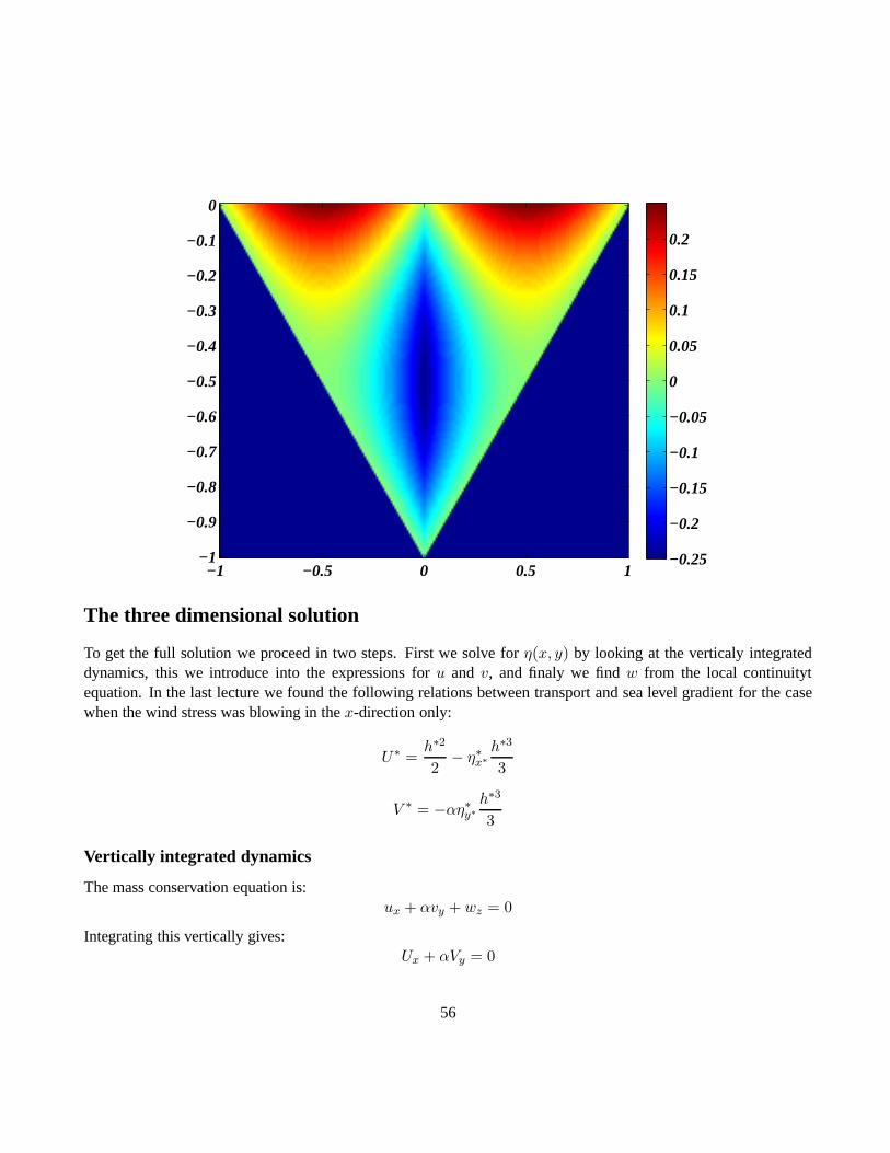
so that at the end of the lakeη = 2 10−6 5 103 or about one centimeter!Now we can get the axial velocityu:
u∗ = h∗2(
z2 − 1)
+ h∗ (z + 1)
Here is a map ofu∗ on ay∗, z∗ section.On the right, for smallh, the flow is just like Couette flow, but on the left, the flow is more like the flow forced
by a pressure gradient between two parallel plates.HOMEWORK FOR THURSDAY: make similar maps forh∗ = exp−6y∗2 andh∗ = (1 − y∗2)
55
−1 −0.5 0 0.5 1−1
−0.9
−0.8
−0.7
−0.6
−0.5
−0.4
−0.3
−0.2
−0.1
0
−0.25
−0.2
−0.15
−0.1
−0.05
0
0.05
0.1
0.15
0.2
The three dimensional solution
To get the full solution we proceed in two steps. First we solve for η(x, y) by looking at the verticaly integrateddynamics, this we introduce into the expressions foru and v, and finaly we findw from the local continuitytequation. In the last lecture we found the following relations between transport and sea level gradient for the casewhen the wind stress was blowing in thex-direction only:
U∗ =h∗2
2− η∗x∗
h∗3
3
V ∗ = −αη∗y∗h∗3
3
Vertically integrated dynamics
The mass conservation equation is:ux + αvy + wz = 0
Integrating this vertically gives:Ux + αVy = 0
56

This condition guarantees the existence of a “transport streamfunction”ψ defined as:
U = −ψy αV = ψx
The analogy with the streamfunction is obvious: lines of constantψ are everywhere parallel to the transport vector,and soψ must be constant along the boundaries. We can then write the equations for the transport as:
ηx =3
h3ψy +
3
2h
ηy = − 3
α2h3ψx
Solution for the transport streamfunction
Then cross-differentiate and subtractto eliminateη, and get an quation forψ:(
ψxα2h3
)
x+
(
ψyh3
)
y= −
(
1
2h
)
y=
hy2h2
Whenh = h(y)
ψxxα2
+ h3(
ψyh3
)
y=hhy2
the boundary condition is thatψ = 0 on all boundaries. Note that in theMathieu et al.paper, the sign on the rightis the opposite, because their definition ofψ is the opposite of ours. Also, thetxS in their paper is1 here, since wehave assume the wind stress is constant. The PDE is elliptic
Near mid-basin (x = 0), we expectψx = ψxx = 0. If ψ∞ represents the solution in that region, then it solves:
(
ψ∞
y
h3
)
y=
hy2h2
= −(
1
2h
)
y
This can be integrated once to give
ψ∞
y =h2
2+ Ch3
The constant C is evaluated by imposing the condition thatψ∞ = 0 on both sides of the basin, givingC = 2/3, fora linearly sloping bottom (< h2 >= 1/3 and< h3 >= 1/4). Comparison with the expression forU shows thatthis corresponds toηx = 2, so this is the same solution as we found before.
In the rest of the basin, we want to find a solution of the form
ψ =∞∑
n=0
anXn(x)Yn(y)
57

One way to do this is to define theYn’s as solutions to:
d
dy
(
1
h3
dYndy
)
+λnh3Yn = 0
with homogeneous boundary conditions:Yn(y = ±1) = 0.This is useful because the differential equation
d
dx
(
p(x)dYndx
)
+ (q(x) + λnr(x))Yn = 0
with homogeneous boundary conditions atx = a, b is called a Sturm-Liouville system. The solutions (Yn) form anorthonormal, or complete set of functions. Any function canbe written as
f(x) =∞∑
n=0
anYn(x)
and normalized such that∫ b
ar(x)YnYmdx = δnm
The easiest way to findYn is to make afinite differenceanalog to the equation: MORE ON THIS LATER. Hereis what theYn functions look like: With these definitions the equation forψ can be written as:
−1 −0.5 0 0.5 1−1
−0.8
−0.6
−0.4
−0.2
0
0.2
0.4
0.6
0.8
1
y
Yn
∞∑
n=0
anX′′
n(x)Yn(y)
α2h3−
∞∑
n=0
anλnXn(x)Yn(y)
h3=
hy2h2
58
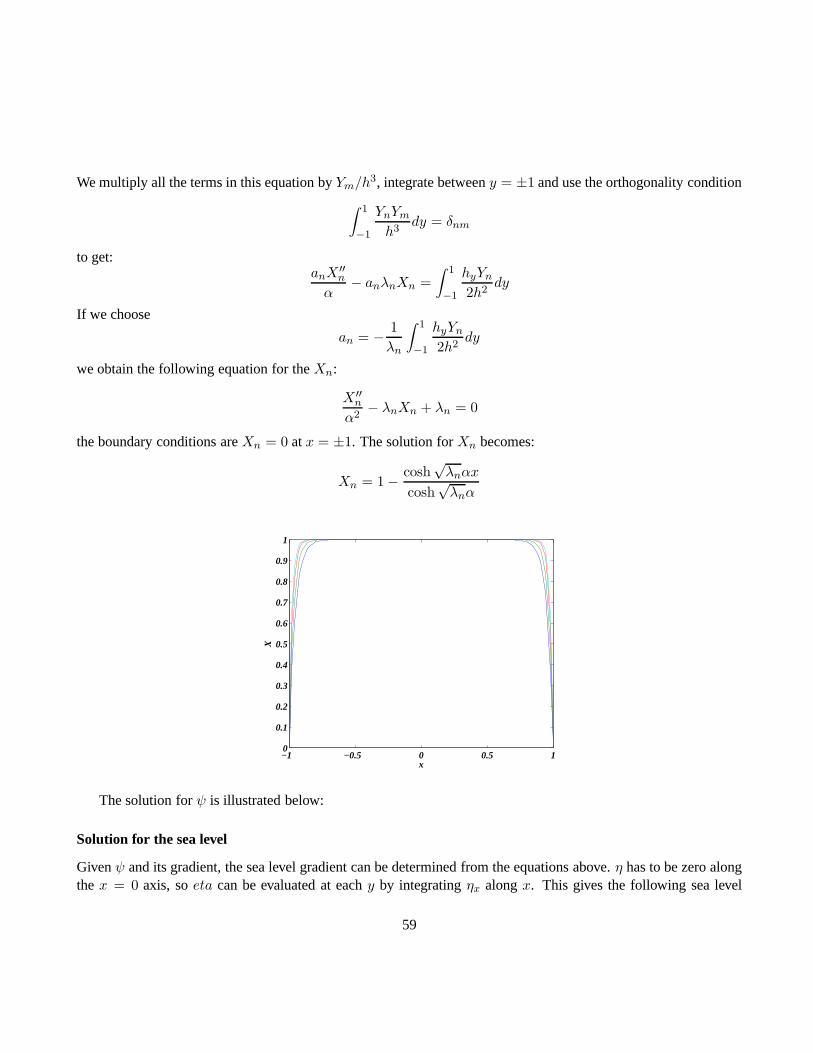
We multiply all the terms in this equation byYm/h3, integrate betweeny = ±1 and use the orthogonality condition
∫ 1
−1
YnYmh3
dy = δnm
to get:anX
′′
n
α− anλnXn =
∫ 1
−1
hyYn2h2
dy
If we choose
an = − 1
λn
∫ 1
−1
hyYn2h2
dy
we obtain the following equation for theXn:
X ′′
n
α2− λnXn + λn = 0
the boundary conditions areXn = 0 atx = ±1. The solution forXn becomes:
Xn = 1 − cosh√λnαx
cosh√λnα
−1 −0.5 0 0.5 10
0.1
0.2
0.3
0.4
0.5
0.6
0.7
0.8
0.9
1
x
X
The solution forψ is illustrated below:
Solution for the sea level
Givenψ and its gradient, the sea level gradient can be determined from the equations above.η has to be zero alongthex = 0 axis, soeta can be evaluated at eachy by integratingηx alongx. This gives the following sea level
59

x
y0.005
0.010.015
−0.015−0.01
−0.005
−1 −0.5 0 0.5 1−1
−0.8
−0.6
−0.4
−0.2
0
0.2
0.4
0.6
0.8
1
−1−0.5
00.5
1
−1−0.5
00.5
1−0.02
−0.01
0
0.01
0.02
xy
ψ
pattern: Alternatively we can take the divergence of the expressions forU andV to obtain a partial differentialequation forη:
Ux = −h3
3ηxx
60

Vy = −αh3
3ηyy − αh2hyηy
ηxx + α2ηyy +3α2hyh
ηy = 0
with boundary conditions:
ηx =3
2hon y = ±1 and ηy = 0 on x = ±L
this is a more difficult problem to solve.
Solution for the vertical velocity
To get the vertical velocity, start from the continuity equation:
wz = −ux − αvy = −z2 − h2
2(ηxx + α2ηyy) + α2hhyηy
or, substituting from the differential equation forη
wz = 3α2hyηyh
z2 − h2
2+ α2hhyηy = α2hhyηy
2
(
3z2
h2− 1
)
Upon integration this gives
w = α2h2hyηy
2
z
h
(
z2
h2− 1
)
which satisfies the boundary condition thatw = 0 at both the bottom and the surface. Plots of the vertical structureof v andw are illustrated for positiveηy below.
The following figure illustrates the three components of thevelocity atx = 0.92 and atx = 0.99.
61

−0.5 −0.4 −0.3 −0.2 −0.1 0 0.1 0.2−1
−0.9
−0.8
−0.7
−0.6
−0.5
−0.4
−0.3
−0.2
−0.1
0
wv
62

−101−1
−0.5
0
−0.2
−0.1
0
0.1
0.2
−1
0
1
x 10−3
−4
−3
−2
−1
0x 10
−3
−101−1
−0.5
0
−0.1
0
0.1
−0.2
−0.1
0
0.1
0.2
−0.4
−0.3
−0.2
−0.1
0
63

Lecture 11
Flow at high Re: Bernouilli
As always, begin with:∇ · u∗ = 0
St∂u∗
∂t∗+ (u∗ · ∇∗)u∗ +
1
Rok × u∗ = −Eu∇∗p∗ +
1
Fr2k +
1
Re∇2u∗
If the Reynolds number is very large,and we are willing to drop the no-slip condition, the dimensional version ofthese equations becomes:
∇ · u = 0
The Bernouilli Equation
Now we consider inviscid flow, when the momentum equation canbe written as:
∂u
∂t+ (u · ∇)u = −∇p
ρ+ g
This is called Euler’s equation. Noting that
(u · ∇)u =1
2∇(u2) − u×∇× u
and withω = ∇× u =, and for a constant density fluid, the momentum equation is
∂u
∂t+
1
2∇(u2) − u× ω = −1
ρ∇(p+ ρgz)
Look at components of this equation along and normal to streamlines:ω is perpendicular tou, so the componentof the momentum equation along a streamline can be writen:
∂u
∂t+
∂
∂s
(
1
2u2 +
p
ρ+ gz
)
= 0
64

wheres represents distance along a streamline. The component normal to the streamline is:
u∂v
∂s= −1
ρ
∂(p + ρgz)
∂n
which shows that for a flow to change direction, the pressure must be different in the direction normal to thestreamline.
Steady Flow
For steady flow, the inviscid momentum equation can be integrated between any points on a streamline with theresult that
1
2u2 +
p
ρ+ gz = B(ψ)
in words, the expression on the left hand side is a constant along the streamline. This is Bernouilli’s equation forsteady, inviscid, rotational flow.
Unteady Flow
The equivalent expression for unsteady flow is:
∫ 2
1
∂u
∂tds+
1
2u2
2 +p2
ρ+ gz2 =
1
2u2
1 +p1
ρ+ gz1
where the integral on the left hand side is the integral between two points1 and2 on the same streamline of theaccelaration. This expression takes on a particularly useful form in the case of irrotational flow (ω = 0). In thatcase, the velocity can be written as the gradient of the so-called velocity potentialu = ∇φ. This is a very strongrestriction on the velocity field. In that case the unsteady momentum equation becomes:
∇(
φt +1
2u2 +
p
ρ+ gz
)
= 0
This can then be integrated in space to give:
φt +1
2u2 +
p
ρ+ gz = f(t)
and since we are only interested in gradients inφ, we can without loss of generality takef(t) = 0. So the lefthand side is zero everywhere in an irrotational inviscid unsteady fluid. This is Bernouilli’s equation for unsteady,inviscid, irrotational flow.
65

Examples
Convergent section: the Venturi
Assume thatz is the same in both problems
Q = U1A1 = U2A2
p1 +ρU2
1
2= p2 +
ρU22
2
p1 − p2 =ρ
2(U2
2 − U21 ) = ρ
U22
2
(
1 − A22
A21
)
or in terms ofQ:
p1 − p2 = ρQ2
2A22
(
1 − A22
A21
)
The primary use of the Venturi is to measure flow rate.
Pitot tube
pt = ps + ρU2
2
so the velocity is given by
U =
√
2(pt − ps)
ρ
Leaky tank
Define two points, the first,1 located at the free surface and the other2 locate in the middle of the orifice. Theheight of the water in the tank ish. First assume the flow is steady. Along a streamline
p1 +ρU2
1
2+ ρgh = p2 +
ρU22
2
butp1 = p2, then solve the above forU2:
U2 =
√
2gh
1 −A22/A
21
66
Faucet
The first point is where the faucet opens to the atmosphere, and the second point is some length h beneath the first.The pressure outside the flowing water is constant, and because the flow is straight, the pressure has to be constantat any value of h, sop1 = p2.
ρU21
2+ ρgh =
ρU22
2
Sluice gate
U-tube
The fluid in one arm has heightl1 and in the otherl1. Define points1 and2 at the two surfaces. The unsteady formof Bernouilli’s equation gives:
∫ 2
1
∂U
∂tds+
1
2U2
2 + gl2 =1
2U2
1 + gl1
because the pressure is the same at the surface. If the diameter of the tube is constant,U is as well, the equationreduces to:
(l1 + l2)dU
dt= g(l1 − l2)
or, with l = l1 + l2, andU = dl2/dtd2l2dt
+2gl2l
= g
This is the equation for a harmonic oscillator with frequency√
2g/l.
Unsteady leaky tank
67

Lecture 12
Potential Flow
As always, begin with:∇ · u = 0
It can be verified that if∇× u + 0
the velocity can be defined as the gradient of a potentisl:
u = ∇φ
then the governing equation forφ comes directly from ccontinuity:
∇ · ∇φ = ∇2φ = 0
This is another elliptic pde, so required boundary conditions are that the normal component ofφ vanish at theboundary. For a 2-d (can be extended to axisymmetric) flow, a streamfunction can be defined as
u = −∂ψ∂y
v =∂ψ
∂x
The condition that the vorticity be zero then gives:
∇2ψ = 0
so that both the stream and potential functions satisfy Laplace’s equation.
Flow around a cylinder
Make coord system sketch
68

In cylindrical polar coordinates (x, r, θ) Laplace’s equation is
∇2φ =1
r
∂
∂r
(
r∂φ
∂r
)
+1
r2∂2φ
∂θ2+∂2φ
∂x2
In this problem there is no variation inx. Then the equation becomes:
∂2φ
∂r2+
1
r
∂φ
∂r+
1
r2∂2φ
∂θ2= 0
The boundary conditions are that there be noflow through the surface of the cylinder (r = a): φr = 0 and that faraway from the cylinder the velocity is uniform and along the x-axis:
ur = U cos θ uθ = −U sin θ
∂φ
∂r= U cos θ
In terms of the streamfunction, atr = a, ψ = 0 while for larger, ψ = Ur sin θIf we write φ = R(r)Θ(θ) and multiply the equation byr2/φ:
r2
R
∂2R
∂r2+r
R
∂R
∂r+
1
Θ
∂2Θ
∂θ2= 0
r2
R
∂2R
∂r2+r
R
∂R
∂r= − 1
Θ
∂2Θ
∂θ2= k2
where the choice ofk2 anticipates that the solution must be periodic inθ. This separates out as:
r2∂2R
∂r2+ r
∂R
∂r− k2R = 0
and∂2Θ
∂r2+ k2Θ = 0
The general solution forRk is:Rk = bkr
k + ckr−k
Θ = dk cos kθ + ek sin kθ
∂φ
∂r=∑
k(bkrk−1 − ckr
−k−1)(dk cos kθ + ek sin kθ)
Far from the sphere the bc is∂φ
∂r= U cos θ
69

this means that we have to choosek = 1 only, b1d1 = U ande1 = 0. and on the sphere
φr = 0
This meansc1 = b1a2 So the overall solution is
φ = U
(
r +a2
r
)
cos θ
and for the streamfunction:
ψ = U
(
r − a2
r
)
sin θ
In terms of velocities:
ur = U
(
1 − a2
r2
)
cos θ
uθ = −U(
1 +a2
r2
)
sin θ
Figure At the surface of the cylinderuθ = −2U sin θ, and we can get the pressure for Bernouilli’s equation:
p(a, θ) = p∞ + ρU2
2(1 − 4 sin2 θ)
In non-dimensional terms
Cp =p(a, θ) − p∞
ρU2
2
= 1 − 4 sin2 θ
The complex plane
For 2-d flows (this works for axisymmetric flows as well), we define a new independant variable:z = x+ iy. Nowconsider a general complex functions:
W (z) = φ+ iψ
and look at
∇2W =∂2W
∂x2+∂2W
∂y2=d2W
dz2
(
∂z
∂x
)2
+d2W
dz2
(
∂z
∂y
)2
but∂z/∂x = 1 and∂z/∂y = i so(∂z/∂y)2 = −1
∇2W = 0 = ∇2φ = ∇2ψ.
70
Another aspect of this is that we want the derivativeW ′ = dW/dz to not depend on the direction in the z-planethat the derivative is taken. Ifz ‖ x,
dW
dz=∂φ
∂x+ i
∂ψ
∂x
if z ⊥ x,dW
dz=
1
i
∂φ
∂y+∂ψ
∂y= −i∂φ
∂y+∂ψ
∂y
for these two values of to be equal, the Cauchy-Riemann conditions have to be satisfied:
∂φ
∂x=∂ψ
∂y
and∂φ
∂y= −∂ψ
∂x.
So ANY function we can write asW = W (z) as opposed toW = W (x, y) provides two solutions to Laplace’sequations. We this in mind we can build a catalog of solutions, and see what flows they correspond to, or equiv-alently what boundary conditions they satisfy. One boundary condition is that the velocity normal to a boundarymust be zero. Note that this is equivalent to saying that any streamline can be a boundary.
Flows without Circulation
1. Streaming;W = Uz u = U , a constant
2. Corner Flows:W = Uzn;n > 0W = Arn(cosnθ + i sinnθ)
φ = Arn cosnθ ψ = Arn sinnθ
The body can be found byψ = 0 onθ = 0, π/n.
3. Sources and Sinks:
W =k
2πlnz =
k
2πlnr + i
kθ
2π
then
ur =∂φ
∂r=
k
2πruθ = 0
This represents a flow that extends radially out from the origin. The source strength is given by:
Q =
∫ 2π
0urrdθ = k
71

4. Doublet:W = Cz−1
The doublet comes about by letting a source and a sink of equalstrength come together at the origin, in sucha way that the product of the source strength time the separation remains finite:
5. Half body:
W = Uz +k
2πlnz + a
ψ = Ur sin θ +kθ
2π
There is a stagnation point on thex axis, a distancea from the origin, wherek/2πa = U The equation forthe streamline that passes through the stagnation point is:
ψb = Ur sin θ +kθ
2π=k
2
6. Rankine Bodies:
W = Uz +k
2πlnz + a − k
2πlnz − a
7. Cylinder:
W = Uz + Ua2
z
The real part is:
φ = U
(
r +a2
r
)
cos θ
as before.
Flows with Circulation
1. Point Vortex:
W =iΓ
2πlnz = − iΓ
2πlnr +
Γθ
2π
Note that the potential function is not unique, it increase by an incrementΓ every timeθ increases by2π. Theradial velocity is every where zero and
uθ =Γ
2πr
This represents a flow that circulates radially around the origin. A measure of the strength of the circulationsis:
∫ 2π
0urrdθ = Γ
72

This flow lookslike it ought to have vorticity. In a polar coordiante systemthex component of vorticity (outof the plane) is:
ω =1
r
∂(ruθ∂r
− 1
r
∂ur∂θ
= 0
But note that the flow is singular atr = 0, and a careful analysis shows that the vorticity is infinite there. Tosee that consider the following:
2. Rankine Combined Vortexuθ = kr r ≤ r0
and
uθ =kr20r
r ≥ r0
This is a combination on solid body rotation forr ≤ r0 and a Point Vortex forr ≥ r0. In the solid bodyrotation portion of the flow,ω = 2k, so this portion of the flow is not potential. Next consider what happensasr0 → 0, andk is increased such that the productkr20 is kept constant, the entire flow becomes irrotationalexcept at the origin, this is the same flow as the Point Vortex descried earlier. The Combine Vortex is oftentaken as a very simple model for a tornado.
3. Images. This method comes in useful when trying to accomodate certain boundary conditions. Considerfor example the case when a Point Vortex is located at some finite distance from a wall. The Point Vortexpotential by itself does not satisfy the boundary conditionof no flow normal to the wall, however considerthe potential
W =iΓ
2πln(z − h) − iΓ
2πln(z + h)
The velocities corresponding to each vortex are equal and opposite along the imaginary axis, and so thevelocity normal to the axis is zero, and that axis becomes a streamline. The addition of animagevortex atz = −h has made it possible to accomodate the boundary. It is important to note that each vortex inducesa velocityux = Γ/4πh at the location of the other vortex, and this has to be interpreted so mean that bothvortices will move in time with that velocity. This result isused to explain why a vortex pair, or a vortex ringwill move through a fluid that is otherwise at rest.
4. Lifting Cylinder:
W = Uz + Ua2
z+iΓ
2πln z
The streamfunction is
ψ = U
(
r − a2)
r
)
sin θ +Γ
2πln r
and the velocities are:
ur = U
(
1 − a2
r2
)
cos θ
73

uθ = −U(
1 +a2)
r2
)
sin θ − Γ
2πr
Compared to the solution without rotation, only the tangential velocity is changed. This affects the locationof the stagnation points. If they are on the body, they will belocated where
sin θ =Γ
4πU
and while still being symmetric fore and aft, we see that the solution above thex axis no longer mirrors thesolution beneath the axis. In general the pressure distribution is no longer symmetric and there can be a netforce acting perpendicular to the free stream. This is called a lift The pressure on the cylinder is given byBernouilli’s equation:
p|r=a = p∞ +1
2ρ
[
U2 −(
−2U sin θ − Γ
2πa
)2]
The lift L is then determined by integrating the pressure around the periphery of the cylinder with the resultthat
L = ρUΓ
This very simple result can be shown to hold trueindependantof the actual shape of the body, and is know asthe Kutta Zhukhowski Lift Theorem. Zhukhowski used this in the early 1900’s to explain how airfoils couldgenerate lift and support the weight of an airplane. Note that the force parallel to the free stream, theDrag isstill zero for these flows.
Discussion of Lift
Consider the flow around an elongated ellipse:
Now consider the same flow when the stream is not aligned with the major axis of the ellipse, but offset byanangle of attackα.
In this solution, the stagnation points are located at pointother than where the major axis intercepts the body.Kutta and Zhukhowski argued that observations never showedthe flow behaved like this, but that because ofother factors (viscosity), the rear stagnation point is always located where the major axis intercepts the ellipseon the lee side of the flow. They suggested that potential flow could be reconciled with the observations ifa just enough circulation was added to the solution to move the lee stagnation point by the right amount.Then they reasoned that the lift on the airfoil could be evaluated using the theorem that bears their name.Experiments suggest that this actually works surprisinglywell, as long asα is kep small. Typically smalmeans less that six or svem degrees, or so long as the observedflow does not separate from the top of theairfoil, a condition known asstall.
74

Lecture 13
Vorticity and the Vorticity Equation
Vorticity
Need a figure
The derivation of the shear deformation can be used to define the rotation of a fluid parcel: for instance therotation along the z-axis is given by
rk =d
dt(φ1 + φ2) =
1
2
(
∂v
∂x− ∂u
∂y
)
wherer is a vector.
More usefully, we define the vortivity vector,ω as twice the rotation rate:
ω1 =
(
∂w
∂y− ∂v
∂z
)
ω2 =
(
∂u
∂z− ∂w
∂x
)
ω3 =
(
∂v
∂x− ∂u
∂y
)
or: ω = ∇× u, the vorticity is the curl of the velocity.
Note that since the vorticity is a curl, it must be divergencefree:
∇ · ω = 0
75

Circulation
Another measure of rotation is the circulation, defined as
Γ =
∫
Aω · nda =
∫
u · ds
Kelvin’s theorem states that for an inviscid fluid
DΓ
Dt= 0
Vortex lines and vortex tubes
Just as streamlines were defined to be lines that are everywhere parallel to the velocity vector, vortex linesare defined to be everywhere parallel to the vorticity vector. The following are a few examples:
(a) In Couette flow the vorticity is−U/h, constant everywhere. The vortex lines are perpendicular to theplane of the flow, and equidistant.
(b) For Poiseuille flow the vorticity is , zero at the center ofthe pipe, and maximum near the walls. Vortexlines are concentric circles, spaced more densely near the outer edge of the flow.
(c) For the Point vortex, there is one isolated vortex line atthe origin.
(d) For solid body rotation, the vorticity is uniform everywhere.
(e) In the Idealized tornado, the vorticity is uniform within the core and zero outside.
Helmholtz proved the following
(a) vortex lines move with the fluid.
(b) the circulation along a vortex tube is constant along itslength
(c) a vortex tube cannot end at a solid boundary. Single vortex lines can, but in general, vortex tubes formclosed loops within the fluid.
The vorticity equation
Sinve vorticity is the curl of the velocity, we can obtain an equation for vorticity by taking the curl of bothsides of the momentum equation:
∇×(
Du
Dt
)
= ∇×(
−∇pρ
+ g + ν∇2u
)
76

First work on the left hand side:
∇×(
Du
Dt
)
=∂
∂t(∇× u) + ∇× [(u · ∇)u]
with
(u · ∇)u =1
2∇u2 − u× (∇× u)
and since the curl of any gradient is zero, the left hand side becomes:
∇×(
Du
Dt
)
=∂
∂t(∇× u) −∇× u× ω
an expression for the curl of the cross product between two vectors gives:
∇× u× ω = (ω · ∇)u − (u · ∇)ω + u(∇ · ω) − ω(∇ · u)
For incompressible flow the last two terms are zero, and so theleft hand side is:
∇×(
Du
Dt
)
=∂ω
∂t+ (u · ∇)ω − (ω · ∇)u =
Dω
Dt− (ω · ∇)u
The right hand side is:
∇×(
−∇pρ
+ g + ν∇2u
)
= −1
ρ∇×∇p+
1
ρ2∇ρ×∇p+ ν∇×∇2u
The first term on the right is zero because it is the curl of a gradient, then:
∇2u = ∇(∇ · u) −∇×∇× u = −∇× ω
and∇×∇2u = −∇×∇× ω = −∇(∇ · ω) + ∇2ω
so the right hand side is:1
ρ2∇ρ×∇p+ ν∇2ω
The vorticity equation is then:
Dω
Dt= (ω · ∇)u +
1
ρ2∇ρ×∇p+ ν∇2ω
If the effect of the earth’s rotation had been included in themomentum equation we would have:
Dω
Dt= [(ω + 2Ω) · ∇]u +
1
ρ2∇ρ×∇p+ ν∇2ω
There are three ways of changing the vorticity of a fluid parcel: the first is when vortex lines are stretched,the second is when constant density and constant pressure lines are not parallel, and the thirs is by diffusion.
77

The stretching of vortex lines
Consider the first mechanism alone, we can write the vorticity equation as:
Dω
Dt= (ω · ∇)u
The factorω · ∇ means the spatial gradient in the direction of the vorticity. If the velocity is not constantin this direction, the vortex lines are strained. If the resulting deformation stretches the vortex lines, thenthe vorticity must increase (to conserve angular momentum), and the opposite is true if the vortex lines arecompressed.
Baroclinic generation
Dω
Dt=
1
ρ2∇ρ×∇p
Isolate a small circular fluid element. The sum of the pressure forces will act through the center of the circle.If the density is not constant and the density lines are not parallel to the pressure lines, the center of gravitywill not lie beneath the center of pressure and a torque will exist in the sense to generate vorticity.
Diffusion of vorticity
Dω
Dt= ν∇2ω
If shear stresses exist, acting on the periphery of a fluid element, then they can add up to produce a torque.
Vorticity generation in a constant density flow
In a constant density flow, the vorticity equation is:
Dω
Dt= (ω · ∇)u + ν∇2ω
There are no source terms on the right, in the sense that if= 0 everywhere, thenDω/Dt = 0 as well. Thisleads to the conclusion that without sources of vorticity atthe boundaries, the vorticity of a flow acceleratedfrom rest would have to remain zero. How might the boundariesproduce vorticity?
78

Consider the flow very near the surface of a solid boundary, inthe presence of a pressure gradient. Thecomponent of the momentum equation parallel to the surface is
∂us∂t
+ us∂us∂s
+ un∂us∂n
= −1
ρ
∂p
∂s+ ν
(
∂2us∂s2
+∂2us∂n2
)
In the limit ass→ 0, all the terms on the left go to zero, and the momentum balancereduces to:
0 = −1
ρ
∂p
∂s+ ν
∂2us∂n2
near the surface,ω = ∂us/∂n, so the boundary condition at the wall is:
µ∂ω
∂n=∂p
∂s
The pressure gradients acts like a vorticity source. Consider how this works on a plate that has a small bluntnose:
79

Lecture 14
Viscous Flows at High Reynolds Number
The Boundary Layer Equations
Prandtl’s central idea was the realization that whenRe ≫ 1 the length scale in the direction normal tothe flow will be smaller than in the direction parallel to the flow, so that the potential flow solution will bemodified to accomodate the no-slip condition in a thin layer (usually, not always) called the boundary layerFor two-dimensional, steady flow
Equations of motion along and perpendicular to the boundary
∂u
∂x+∂v
∂y= 0
u∂u
∂x+ v
∂u
∂y= −1
ρ
∂p
∂x+ ν
(
∂2u
∂x2+∂2u
∂y2
)
u∂v
∂x+ v
∂v
∂y= −1
ρ
∂p
∂y+ ν
(
∂2v
∂x2+∂2v
∂y2
)
Introduce non-fimensional variables:
x∗ = x/L, y∗ = y/δ, u∗ = u/U, v∗ = v/V, p∗ = p/ρU2
Then the continuity equation becomes:
U
L
∂u∗
∂x∗+V
δ
∂v∗
∂y∗= 0
from which we conclude
V ≈ Uδ
L
80

The two components of the momentum equation become:
u∗∂u∗
∂x∗+ v∗
∂u∗
∂y∗= −∂p
∗
∂x∗+
1
Re
∂2u∗
∂x∗2+
1
Re
L2
δ2∂2u∗
∂y∗2
δ2
L2
(
u∗∂v∗
∂x∗+ v∗
∂v∗
∂y∗
)
= −∂p∗
∂y∗+δ2
L2
1
Re
∂2u∗
∂x∗2+
1
Re
∂2u∗
∂y∗2
The first equation suggests that we can retain the higher order derivative at the same time asRe → 0, if wechoose
δ ≈ LRe−1/2
With that choice, they momentum equation becomes simplyp∗y∗ = 0. A cocnsistent set of approxiamtionsleads us to conclude that
(a) p∗ is invariant across the boundary layer.
(b) p∗x∗ can therefore be evaluated at any value ofy∗
(c) A particularly simple place will be at the outer edge of the boundary layer, where the boundary layersolution merges into the outer (potential) flow.
The Streamfunction
The number of independant variables can be reduced, while satisfying the continuity equation if we relatevelocities by the streamfunction, defined as:
u =∂ψ
∂y∗, v = − ∂ψ
∂x∗
The streamwise momentum equation becomes:
ψy∗ψx∗y∗ − ψx∗ψy∗y∗ = px|oe + ψy∗y∗y∗
The equation is third order, and the boundary conditions are:
ψ∗
x = ψ∗
y = 0, at y∗ = 0
andψy ∗ → U(x), at y∗ → ∞
where U(x) represents the velocity at the outer edge of the boundary layer.
The method of solution then consists of first finding the potential flow solution valid outside the area close tothe body, then solving the boundary layer equation, subjectto the conditions listed above.
81

Lecture 15
Laminar Boundary Layer on a Solid Surface
The Flat Plate
The potential flow induced by a uniform stream (velocity=U ) over a plate aligned with the flow is particularlysimple. Since the boundary condition of no flow perpendicular to the plate is atisfied by the streaming flow,the potential flow over the plate has constant velocity, Bernouilli’s equation then insures that the pressure isconstant and so the streamwise pressure gradient is zero everywhere, and the forcing term in the boundarylayer equation is zero. The boundary layer equation is then:
ψy∗ψx∗y∗ − ψx∗ψy∗y∗ = ψy∗y∗y∗
with boundary conditions:ψx∗ = ψy∗ = 0 at y∗ = 0
ψy∗ = 1 as y∗ =→ ∞The method of solutions consists of transforming the partial differential equation into an ordinary differentialequation, this is called asimilsrity transformation. This approach is similar to what we did whenwe workedout the solution to the impulsively started flat plate, in viscous flow. Try
η = Axpy
thendη
dx= Apxp−1y = p
η
x
dη
dy= Axp
82

Sinceu∗ → 1 asy∗ becomes large, independant ofx∗, it seems a good idea to define as a new dependantvariable
u∗ = ψy∗ =df
dη= f ′(η)
then
ψ =
∫
df
dηdy =
dy
dη
∫
df
dηdη = A−1x−pf(η)
andψx∗ = −A−1px−p−1f +A−1px−p−1ηf ′ = A−1px−p−1(ηf ′ − f)
ψx∗y∗ = pη
xf ′′
ψy∗y∗ = Axpf ′′
ψy∗y∗y∗ = A2x2pf ′′′
Introducing the new variables into the boundary layer equation gives:
pη
xf ′f ′′ − xppx−p−1(ηf ′ − ff ′′ = A2x2pf ′′′
orp
xff ′′ = A2x2pf ′′′0
If we pick p = −1/2, the equation becomes independant of x, and if we pickA = 1, the expression for thenew independant variable is:
η =y∗√x∗
and the equation becomes2f ′′′ + ff ′′ = 0
In terms of the new variables, the boundary conditions are:
f ′ = f = 0 at η = 0
f ′ = 1 as η → ∞The equation is non-linear and can be solved numerically using a method known asShooting. Imagine thatinstead of the boundary condition atη → ∞, we knew a third conditon atη = 0, sayf ′′(0) = 1. Thenthe equation could be numerically integrated away from zero, by quadrature or some other method. Turn thethird order differential equation into a system of three first order equations:
g = f ′ h = g′ = f ′′ 2h′ = −fh
If we have initial conditions, for instance atη = 0, these equations can be integrated numerically by someappropriate scheme. One important concept here is that in practice the bc at infinity can be applied at some
83

finite value ofη, although just what that value is may require some experimentation. Typically, for boundarylayer calculations, integrating out toη∞ = 10 is sufficient. If theη axis is discretized intoN segements, thesimplest quadrature scheme would say:
fn+1 = fn + gnδη
gn+1 = gn + hnδη
hn+1 = hn −fnhn
2δη
The first integration is carried out with an initial guess athn(1), and the result forgN is compared to therequired value of1. If the computedgN is too large, then a new initial guess, smaller than the first is tried. Ifthe new guess give a value ofgN that is too small another guess is made, and the process is repeated until theboundary condition away from the plate is met. Blasius foundthat the value off ′′(0) that results inf ′ tendingto one for largeη is 0.3321. The results are slightly sensitive to the choice of N andη∞. The computedf ′ isillustrated in Fig.
For practical purposes, the viscous effects are seen to be confined within a region that extends out toηoe = 6.to return to physical space
y∗oe√x∗
=
√L
δ
δoe√x
=
√
U
ν
δoe√x
= 6
and this gives and expression for the boundary layer thickness:
δoe =
√
νx
U
The stress at the wall is:
τw = µ∂u
∂y|y=0 = µU
√
U
νxf ′′(0) = 0.3321µ
√
U3
νx
Stagnation Point Flow
As a first example of a flow where the pressure gradient forcingis important consider the flow near thestagnation point of a cylinder in a flow that has a uniform velocity upstream equal toU . The potential flowsolution for the tangential velocity is:
Uoe(x) = −2U sin θ ≈ 2Ux
R
and the pressure
poe = p∞ +ρU2
2− 2ρU2x2
R2
84

so the pressure gradient in boundary layer variables is:
p∗x|oe = 4x∗
u∂u
∂x+ v
∂u
∂y= 4
U20
R2x+ ν
∂2u
∂y2.
η =Ay
xn, ψ = BxmF (η)
d3F
dη3+ F
d2F
∂η2−(
dF
dη
)2
+ 1 = 0
.
Flow over a Wedge
85

Lecture 16
Free Shear Flows
86