AN INTRODUCTION TO FLAG MANIFOLDS

Notes1 for the Summer School on Combinatorial Models in Geometry andTopology of Flag Manifolds, Regina 2007

1. The manifold of flags

The (complex) full flag manifold is the space Fn consisting of all sequences

V1 ⊂ V2 ⊂ . . . ⊂ Vn = Cn

where Vj is a complex linear subspace of Cn, dim Vj = j, for all j = 1, . . . , n (such sequences

are sometimes called flags in Cn). The manifold structure of Fn arises from the fact that thegeneral linear group GLn(C) acts transitively on it: by this we mean that for any sequenceV• like above, there exists an n × n matrix g which maps the standard flag

SpanC(e1) ⊂ SpanC(e1, e2) ⊂ . . . ⊂ Cn

to the flag V• (here e1, . . . , en is the standard basis of Cn). That is, we have

(1) g(SpanC(e1, . . . , ej)) = Vj,

for all j = 1, 2, . . . , n − 1 . In fact, if we return to (1) we see that we can choose the matrixg such that ge1, ge2, . . . , gen is an orthonormal basis of Cn with respect to the standardHermitean product 〈 , 〉 on C

n; the latter is given by

〈∑

j

ζjej ,∑

j

ξjej〉 :=∑

j

ζjξj,

for any two vectors ζ =∑

j ζjej and ξ =∑

j ξjej ∈ Cn. In other words, g satisfies

〈gζ, gξ〉 = 〈ζ, ξ〉

for all ζ, ξ ∈ Cn; so g is an element of the unitary group U(n).

In conclusion: flags can be identified with elements of the group GLn(C), respectivelyU(n), modulo their subgroup which leave the standard flag fixed. The two subgroups canbe described as follows:

• for the GLn(C) action, the group Bn of all upper triangular (invertible) matrices withcoefficients in C

• for the U(n) action, the group T n of all diagonal matrices in U(n); more specifically,T n consists of all matrices of the form

Diag(z1, z2, . . . , zn)

where zj ∈ C, |zj| = 1, j = 1, 2, . . . , n, which means that T n can be identified withthe direct product (S1)×n; we say that T is an n-torus.

This implies that Fn can be written as

Fn = GLn(C)/Bn = U(n)/T n

so it is what we call a homogeneous manifold ( for more explanations, see Section 2, theparagraph after Definition 2.4).

Another related space is the Grassmannian Grk(Cn) which consists of all complex linear

subspacesV ⊂ C

n

1I am indebted to Leonardo Mihalcea and Matthieu Willems for helping me prepare these notes.1

2

with dim V = k. The spaces Fn and Grk(Cn) are the two extremes of the following class of

spaces: fix 0 ≤ k1 < k2 < . . . < kp ≤ n and consider the space Fk1,...,kpwhich consists of all

sequencesV1 ⊂ V2 ⊂ . . . ⊂ Vp ⊂ C

n

with dim Vj = kj, for all j = 1, . . . , p. These spaces are called flag manifolds. Each of themhas a transitive action of U(n) (the arguments we used above for Fn go easily through), sothey are homogeneous manifolds.

There exist also Lie theoretical generalizations of those manifolds. The goal of these notesis to define them and give some basic properties of them. First, we need some backgroundin Lie theory. This is what the next section presents.

2. Lie groups, Lie algebras, and generalized flag manifolds

This is an informal introduction to Lie groups. It is intended to make the topics ofthe School accessible to the participants who never took a course in Lie groups and Liealgebras (but do know some point-set topology and some basic notions about differentiable2

manifolds).

Definition 2.1. A Lie group is a subgroup of some general linear group GLn(R) which is aclosed subspace.

Note. For people who know Lie theory: the groups defined here are actually “matrix Liegroups”. These are just a special class of Lie groups. However, unless otherwise specified,no other Lie groups will occur in these notes and probably also in the School’s lectures.

We note that GLn(R) has a natural structure of a differentiable manifold (being open

in the space Matn×n(R) ≃ Rn2

of all n × n matrices – why?). Moreover, the basic groupoperations, namely multiplication

GLn(R) × GLn(R) ∋ (g1, g2) 7→ g1g2 ∈ GLn(R)

and taking the inverseGLn(R) ∋ g 7→ g−1 ∈ GLn(R)

are differentiable maps (why?). Finally, consider the exponential map

exp : Matn×n(R) → GLn(R)

given by

(2) exp(X) =∑

k≥0

1

k!Xk.

The differential of exp at 0 is the identity map on Matn×n(R); consequently exp is a localdiffeomorphism at 0.

An important theorem says that any Lie group G ⊂ GLn(R) like in Definition 2.1 is adifferentiable manifold, actually a submanifold3 of GLn(R). Consequently, the maps

G × G ∋ (g1, g2) 7→ g1g2 ∈ G

andG ∋ g 7→ g−1 ∈ G

2By “differentiable” we always mean “of class C∞”.3For us, submanifolds are closed embedded submanifolds, unless otherwise specified.

3

are differentiable. A proof of this theorem can be found for instance in [Br-tD, Ch. I,Theorem 3.11] or [He, Ch. II, Section 2, Theorem 2.3]. The idea of the proof is to constructfirst a local chart around I: more precisely, one shows that

(3) g := X ∈ Matn×n(R) : exp(tX) ∈ G ∀t ∈ R

is a vector subspace of Matn×n(R). Moreover, exp (see (2)) maps g to G and is a localhomeomorphism at 0: this homeomorphism gives the chart at I; a chart at an arbitrarypoint g is obtained by “multiplying” the previous chart by g. The map

exp : g → G

is called the exponential map of G. The subspace g of Matn×n(R) is called the Lie algebra ofG. It is really an algebra (non-commutative though), with respect to the composition lawdefined in the following lemma.

Lemma 2.2. Let G be a Lie group and g its Lie algebra.

(a) If g is in G and X in g then

Ad(g)X := gXg−1 ∈ g.

(b) If X, Y ∈ g, one has

d

dt|0 exp(tX)Y exp(−tX) = XY − Y X

Consequently, the commutator

[X, Y ] := XY − Y X

is in g.

Proof. Exercise.

The composition law on g we were referring at above is

g × g ∋ (X, Y ) 7→ [X, Y ] ∈ g.

Note that the algebra (g, [ , ]) is not commutative and not associative; instead, the Liebracket operation [ , ] satisfies

[X, Y ] = −[Y, X] (anticommutativity)

[[X, Y ], Z] + [[Z, X], Y ] + [[Y, Z], X] = 0 (Jacobi identity)

for any X, Y, Z ∈ g.

Note. Have you ever seen a composition law with the above properties before? I hopeeveryone remember that the space of vector fields on a manifold M can be equipped witha Lie bracket which satisfies the two properties from above. Namely, if u, v are two vectorfields on M , then the vector field [u, v] is defined by

(4) [u, v]p(ϕ) := up(v(ϕ)) − vp(u(ϕ)),

for any p ∈ M and any germ of real function ϕ (defined on an open neighborhood of p inM). This is called the Lie algebra of vector fields on M and is denoted by X (M).

There is a fundamental question we would like to address at this point: to which extentdoes the Lie group G depend on the surrounding space GLn(R)? Because G can be imbeddedin infinitely many ways in a general linear group: for instance, we have

G ⊂ GLn(R) ⊂ GLn+1(R) ⊂ . . . .

4

All notions defined above — the space g, the map exp : g → G, and the bracket [ , ] — aredefined in terms of GLn(R). In spite of their definition, they actually depend only on themanifold G and the group multiplication (in other words, they are intrinsically associatedto the Lie group G). This is what the following proposition says. First, we say that a vectorfield u on G is a G-invariant vector field if

ug = (dg)I(uI)

for all g ∈ G (here we identify g with the map from G to itself give by left multiplication byg). We denote by XG the space of all G-invariant vector fields on G.

Proposition 2.3. Let G be a Lie group.

(a) The space g is equal to the tangent space TIG of G at the identity element I. The mapg → XG given by

X 7→ [G ∋ g 7→ gX]

is a linear isomorphism.

(b) If X is in g, then the map

R ∋ t 7→ exp(tX)

is the integral curve associated to the (invariant) vector field

G ∋ g 7→ gX.

(c) The space XG is closed under the Lie bracket [ , ] given by (4).

(d) The map

g ∋ X 7→ [G ∋ g 7→ gX]

is a Lie algebra isomorphism (that is, a linear isomorphism which preserves the Lie brackets)between g and XG.

Proof. To prove (a), we note that for any X ∈ g, the assignment R ∋ t 7→ exp(tX) is a curveon G whose tangent vector at t = 0 is

d

dt|0 exp(tX) = X.

The equality follows by dimension reasons.

The only non-trivial remaining point is (d). Namely, we show that if X, Y are in g, thanthe Lie bracket of the vector fields

G ∋ g 7→ gX and G ∋ g 7→ gY

is equal to

G ∋ g 7→ g[X, Y ].

It is sufficient to check that the two vector fields are equal at I. Indeed, the Lie bracket ofthe two vector fields at I evaluated on a real function ϕ defined on a neighborhood of I inG equals to

d

dt|0

d

ds|0[ϕ(exp(tX) exp(sY ))] −

d

dt|0

d

ds|0[ϕ(exp(tY ) exp(sX))],

which is the same as

(dϕ)I(XY − Y X).

The proof is finished (the students are invited to check all missing details).

5

Consequently, if we denote by GL(g) the space of all linear automorphisms of g, then themap

Ad : G → GL(g), g 7→ Ad(g)

(see Lemma 2.2, (b)) is also independent of the choice of GLn(R) in Definition 2.1. The mapAd is called the adjoint representation of G. It can be interpreted as an action of G on g,

that is, it satisfies4

Ad(g1g2)X = Ad(g1)(Ad(g2)X)

Ad(e)X = X,

for all g, g1, g2 ∈ G and all X ∈ g.

In the category of Lie groups, a morphism is a group homomorphism which is also adifferentiable map. An isomorphism is of course a bijective morphism whose inverse is alsoa morphism. Two Lie groups are isomorphic if there exists an isomorphism between them.Proposition 2.3 implies that for Lie groups that are isomorphic, there is a natural way toidentify the adjoint orbits (by identifying first their Lie algebras).

Definition 2.4. A (generalized) flag manifold is an adjoint orbit

Ad(G)X0 := Ad(g)X0 : g ∈ G,

where G is a compact Lie group.

Before seeing examples, we would like to explain the manifold structure of Ad(G)X0. LetGX0

be the G-stabilizer of X0, which consists of all g ∈ G with

Ad(g)X0 = X0.

This is also a closed subgroup of GLn(R), thus a Lie group. Set-theoretical, we can obviouslyidentify

(5) Ad(G)X0 = G/GX0,

where the latter is the space of all cosets gGX0, with g ∈ G. The quotient G/GX0

is ahomogeneous manifold: to define the manifold structure, we consider the Lie algebra gX0

ofGX0

and pick a direct complement of it in g, call it h; that is, we have

g = gX0⊕ h.

For a sufficiently small neighborhood U of 0 in h, the map

U ∋ X 7→ exp(X)GX0∈ G/GX0

is a local chart around the coset IGX0. A chart at an arbitrary point gGX0

is obtained by“multiplying” the previous one by g.

Examples. 1. (R>0, ·) and more generally ((R>0)n, ·) (the multiplication is componentwise)

are Lie groups. Indeed, the latter can be identified with the subgroup of GLn(R) consisting ofdiagonal matrices with all entries strictly positive: the latter is a closed subspace of GLn(R).

2. (R, +) and more generally, (Rn, +) are Lie groups. Because the latter can be identifiedwith the Lie group ((R>0)

n, ·) from the previous example via the exponential map.

3. Consider the circleS1 := z ∈ C | |z| = 1.

4In general, a (smooth) action of a Lie group G on a manifold M is a (differentiable) map G×M →M ,G×M ∋ (g, p) 7→ gp ∈M with the properties Ip = p and g1(g2p) = (g1g2)p, for all p ∈M , g, g1, g2 ∈ G. Ifp ∈M , then orbit of p is Gp := gp : g ∈ G and the stabilizer of p is Gp := g ∈ G : gp = p.

6

The groupT n := (S1)n

is a Lie group, being identified with the subgroup of GLn(C) consisting of

Diag(z1, . . . , zn),

with zk ∈ S1, 1 ≤ k ≤ n. The group T n is called the n-dimensional torus. Note that themap

Rn → T n, (θ1, . . . , θn) 7→ (eiθ1 , . . . , eiθn)

is a group homomorhism, being at the same time a covering map (all pre-images can beidentified with Z).

4. Recall from Section 1 that the unitary group U(n) consists of all n×n matrices g whichpreserve the canonical Hermitean product on Cn. An easy exercise shows that

U(n) = g ∈ Matn×n(C) : g · gT = In.

Show that U(n) is a compact topological subspace of GLn(C) (hint: what are the diagonalelements of the product ggT?). Then show that U(n) is a connected topological subspace ofGLn(C) (hint: consider first the canonical action of U(n) on Cn and note that the orbit ofe1 is the unit sphere S2n−1 and the stabilizer of the same e1 is U(n − 1); this implies thatS2n−1 = U(n)/U(n − 1) is a connected space; use induction by n.) Via the identification5

Matn×n(C) ∋ a + ib =

(

a −bb a

)

∈ Mat2n×2n(R),

U(n) becomes a closed subgroup of GL2n(R), thus a Lie group. By the definition given by(3), its Lie algebra is the space

u(n) := X ∈ Matn×n(C) : X + XT = 0

of all skew-hermitean n× n matrices. We want to describe the corresponding adjoint orbits.A result in linear algebra says that the eigenvalues of a skew-hermitean matrix are purelyimaginary; moreover, any skew-hermitean matrix is U(n)-conjugate to a matrix of the form

X0 = Diag(ix1, ix2, . . . , ixn),

where xj ∈ R, j = 1, 2, . . . , n, such that

x1 ≤ x2 ≤ . . . ≤ xn.

So it is sufficient to describe the orbit of X0. This is obviously the set of all skew-hermiteanmatrices with eigenvalues ix1, ix2 . . . , ixn. For sake of simplicity we assume that

x1 < x2 < . . . < xn.

The orbit of X0 can be identified with the space of all n-tuples (L1, L2, . . . , Ln) of complexlines (one-dimensional complex subspaces) in Cn which are any two orthogonal: that is, toany such n-tuple corresponds the matrix X with eigenvalues ix1, ix2, . . . , ixn and correspond-ing eigenspaces L1, L2, . . . , Ln. Via

(L1, L2, . . . , Ln) 7→ L1 ⊂ L1 ⊕ L2 ⊂ . . . ⊂ L1 ⊕ L2 ⊕ . . . ⊕ Ln = Cn,

the latter space coincides with the manifold Fn defined in section 1. In conclusion, theflag manifolds corresponding to U(n) are the manifolds of flags defined in section 1. Thespecial unitary group is

SU(n) = g ∈ U(n) | det(g) = 1.

5Any matrix a + ib ∈ Matn×n(C) defines an R-linear automorphism of R2n, via (a + ib)(u + iv) =a(u) − b(v) + i(b(u) + a(v)).

7

Its Lie algebra is

su(n) := X ∈ Matn×n(C) : X + XT = 0, Tr(X) = 0,

as one can easily check. We can see by using the same arguments as above that the adjointorbits of SU(n) are the manifolds of flags as well.

5. The orthogonal group O(n) consists of all g ∈ GLn(R) which leave the usual scalarproduct on Rn invariant. Concretely,

O(n) = g ∈ Matn×n(R) : g · gT = I,

so O(n) is a Lie group. It is not connected: indeed, its subgroup

SO(n) := g ∈ O(n) : det(g) = 1

is connected (use the same connectivity argument as for U(n), see above) and O(n) is thedisjoint union of SO(n) and

O−(n) := g ∈ O(n) : det(g) = −1.

The group SO(n) is called the special orthogonal group. It is not difficult to see that it is acompact Lie group. There exist descriptions of its adjoint orbits in terms of flags, similar tothose of U(n). We will not use those in the School, so I just address the interested studentsto [Fu-Ha, p. 383] or [Bi-Ha, p. 7].

6. LetH = a + bi + cj + dk | a, b, c, d ∈ R

denote the (non-commutative) ring of quaternions. This is a real algebra generated by i, j,and k, subject to the relations

i2 = j2 = k2 = −1, ij = k, jk = i, ki = j.

The conjugate of an arbitrary quaternion q = a + bi + cj + dk is by definition

q = a − bi − cj − dk.

Note that we have

q1 · q2 = q2 · q1,

for any q1, q2 ∈ H. For n ≥ 1, we regard Hn as an H-module with multiplication from theright. In this way, any matrix A ∈ Matn×n(H) induces a H-linear transformation of Hn, bythe usual matrix multiplication. Any H-linear transformation of Hn is induced in this way.We identify

Hn = C

n ⊕ jCn ≃ C

2n

via

(6) Hn ∋ u = x + jy 7→ (x, y) ∈ C

n ⊕ Cn,

where x, y are vectors in Cn. The latter is a C-linear isomorphism. Take A ∈ Mat(n× n, H)and write it as

A = B + jC,

where B, C ∈ Mat(n×n, C). The C-linear endomorphism of C2n induced by a is determinedby

(B + jC)(x + jy) = Bx − Cy + j(Cx + By).

We deduce that

(7) Mat(n × n, H) =

(

B −CC B

)

| B, C ∈ Mat(n × n, C).

8

We can easily see that if we denote

J =

(

0 −II 0

)

,

then

Mat(n × n, H) = A ∈ Mat(2n × 2n, C) | AJ = JA.

Now let us consider the pairing ( , ) on Hn given by

(u, v) :=n

∑

ν=1

uν vν = u · v∗,

for all u = (u1, . . . , un) and v = (v1, . . . , vn) in Hn. The symplectic group Sp(n) is defined as

Sp(n) = A ∈ Matn×n(H) | (Au, Av) = (u, v) ∀u, v ∈ Hn.

The condition which characterizes A in Sp(n) can be written as

A · u · v∗ · A∗ = u · v∗

for for all q ∈ H. This is equivalent to

A · q · A∗ = q,

for all q ∈ H. We deduce that an alternative presentation of Sp(n) is

Sp(n) = A ∈ Matn×n(H) | A∗ · A = In.

If we use the identification (6), we can express the pairing of u = x + jy with itself as

(8) ‖u‖2 = (u, u) = (x+jy)·(x∗−jyT ) = xx∗+yyT +j(yx∗−xyT ) = xx∗+yy∗ = ‖x‖2+‖y‖2.

An element A of Mat(n × n, H) is in Sp(n) if and only if

(Au, Au) = (u, u),

for any u ∈ Hn. If we write again

A = B + jC =

(

B −CC B

)

as above, then

‖A(u)‖2 = ‖(B + jC)(x + jy)‖2 = ‖Bx − Cy‖2 + ‖Cx + By‖2 = ‖

(

B −CC B

)

·

(

xy

)

‖2.

We deduce that Sp(n) ⊂ U(2n). In fact, we have

(9) Sp(n) =

(

B −CC B

)

∈ U(2n) = g ∈ U(2n) | g = JgJ−1

Thus Sp(n) is a Lie group. Like in Example 5, descriptions of its adjoint orbits in terms offlags can be found in [Fu-Ha, p. 383] or [Bi-Ha, p. 7].

The groups U(n), SU(n), O(n), SO(n) and Sp(n) are called the classical groups.

9

3. The flag manifold of (g, X0)

By Definition 2.4, a flag manifold is determined by a compact Lie group G and the choiceof an element X0 in its Lie algebra g. In this section we discuss the classification of compactLie groups with the same Lie algebra g. We will see that for all such Lie groups the adjointorbits of X ∈ g are the same. The treatment will be sketchy: the details can be found forinstance in [Kn, Chapter I, Section 11] and/or [He, Chapter II, Section 6].

Definition 3.1. A Lie algebra is a vector subspace g of some Matn×n(R) which is closedunder the operation

Matn×n(R) ∋ X, Y 7→ X · Y − Y · X ∈ Matn×n(R).

We also say that g is a Lie subalgebra of Matn×n(R).

We have seen that to any Lie group G ⊂ GLn(R) corresponds a Lie algebra g ⊂ Matn×n(R).Related to this, we have the following result.

Theorem 3.2. (a) Any Lie algebra g is the Lie algebra of a Lie group G. More specifically ifg ⊂ Matn×n(R) is a Lie subalgebra, then there exists a unique connected immersed subgroupG ⊂ GLn(R) whose Lie algebra is g.

(b) More generally, if the Lie group G has Lie algebra g and h ⊂ g is a Lie subalgebra(that is, a linear subspace closed under [ , ]), then there exists a unique connected immersedsubgroup H ⊂ G with Lie algebra h.

Note. The groups G and H arising at point (a), respectively (b), are not necessarily Liegroups, as defined in Definition 2.1. For example, the Lie algebra of the torus T 2 = S1 × S1

is R2 (abelian). The subspace

h := (αt, βt) : t ∈ R

is a Lie subalgebra (here α and β are two real numbers). The subgroup H prescribed bypoint (b) above is

H = (eiαt, eiβt) : t ∈ R.

One can show that if the ratio α/β is irrational, then H is dense in T 2. So there is no wayof making H into a (closed) matrix Lie group — see also the note following Definition 2.1.In fact such situations occur “rarely”. This is why we will always assume (without proof!)that the subgroups G and H arising at point (a), respectively (b) above are (closed matrix)Lie groups.

In general, there is more than one G with Lie algebra g, as the following example shows.

Example. The center of SU(n) is

Z = ζkI | 0 ≤ k ≤ n − 1,

where ζ := e2πin . Then SU(n)/Z is a Lie group (the map Ad : SU(n) → GL(su(n)) has

kernel equal to Z). Its Lie algebra coincides with the tangent space at the identity; but onecan easily see that the map SU(n) → SU(n)/Z is a local diffeomorphism around I and agroup homomorphism, thus the two spaces have the same tangent space at I, with the sameLie bracket. Finally, note that Z can be chosen to be an arbitrary subgroup of Z(G) (wecall it a central subgroup).

In fact, we can describe exactly all Lie groups with given Lie algebra g, as follows.

10

Theorem 3.3. (a) If g is a Lie algebra, then there exists a unique simply connected Liegroup, call it G, of Lie algebra g.

(b) Any Lie group of Lie algebra g is of the form

G = G/Z,

where Z is a discrete central subgroup of G. The group G is called the universal cover of G.

For us, this result is important for the following application:

Corollary 3.4. Let g be a Lie algebra and X0 an element of g. Then for any Lie group Gwith Lie algebra g, the adjoint orbits Ad(G)X0 and Ad(G)X0 are equal.

Proof. We have G = G/Z, where Z ⊂ G is a central subgroup. For g ∈ G we denote by [g]its coset in G. We have

Ad([g])X =d

dt|0[g][exp(tX)][g−1] =

d

dt|0[g exp(tX)g−1] =

d

dt|0g exp(tX)g−1 = Ad(g)X

where we have identified G and G locally around I.

If we want to restrict ourselves to compact Lie groups, we may face the situation whereG is compact but G is not. For example, the universal cover of G = T n (see Example 3,Section 2) is G = Rn (see Example 2, Section 2). Note however that the torus is not aninteresting example for us, as we have

Ad(T )X0 = X0,

for any X0 in the Lie algebra of T , thus an adjoint orbit consists of only one point. Bycontrary, if G is compact, then any G = G/Z like in the previous proposition is compactas well. The following result shows that we do not lose any generality by considering onlyadjoint orbits of groups that are compact and simply connected.

Theorem 3.5. If G is a compact Lie group, then there exists a compact simply connectedLie group H and a torus T such that

G = (H × T )/Z

where Z is a central discrete subgroup of H × T .

Examples. 1. The group U(n) is not simply connected, for any n ≥ 1. This follows by usingagain the inductive argument from Example 4, Section 2: since S2n−1 is simply connectedfor any n ≥ 2, this shows that the fundamental group of U(n) is the same as the one of U(1).But the latter is nothing but the circle S1 in C, so it’s not simply connected.

2. Like in the previous example, the group SU(n) is simply connected, for any n ≥ 1.This time we note that SU(1) is a point, thus simply connected.

3. Like in the previous example, Sp(n) is simply connected, for any n ≥ 1.

4. The group SO(n) is not simply connected. Again, we rely on the inductive argumentand the fact that the fundamental group of SO(3) is Z/2. The same will be the fundamentalgroup of SO(n) for any n ≥ 3. The case n = 2 is special, since

SO(2) =

(

cos θ sin θsin θ cos θ

)

| θ ∈ R,

which can be identified with S1; the fundamental group is Z.

11

5. We can describe H in Theorem 3.5 for U(n) and SO(n). For U(n), we consider theisomorphism

U(n) ≃ S1 × SU(n)

given bySU(n) × S1 ∋ (A, z) 7→ zA ∈ U(n).

As about SO(n), the situation is very different: namely, there exists a simply connectedgroup, denoted by Spin(n), whose centre Z is isomorphic to Z/2 such that

Spin(n)/Z ≃ SO(n).

We wonder now which are the Lie algebras which correspond via Theorem 3.2 to simplyconnected Lie groups which are compact. There exists an algebraic description of such Liealgebras, which is given in the following theorem. First, if g is an arbitrary Lie algebra, andX is in g, by adX we denote the linear endomorphism of g given by

Y ∋ g 7→ adX(Y ) := [X, Y ].

The Killing form of g is the bilinear form B on g given by

κ(X, Y ) := Tr(adX adY ),

for X, Y ∈ g.

Theorem 3.6. A simply connected Lie group G is compact if and only if its Lie algebra hasstrictly negative definite Killing form.

The conclusion of the section can be formulated as follows:

Any flag manifold is an adjoint orbit of a Lie group whose Lie algebra g has strictlynegative definite Killing form. Any such group is automatically compact and has finitecentre. The adjoint orbit of X ∈ g is the same for any Lie group of Lie algebra g.

4. Structure and classification of Lie algebras with κ < 0

Throughout this section g will denote a Lie algebra whose Killing form κ is strictly negativedefinite. The pairing

g ∋ X, Y 7→ 〈X, Y 〉 := −κ(X, Y )

makes g into a Euclidean space. Moreover, we have

(10) 〈[X, Y ], Z〉 = 〈X, [Y, Z]〉,

for all X, Y, Z ∈ g (check this!). We pick t ⊂ g a maximal abelian subspace (by this we meanthat [X, Y ] = 0, for all X, Y ∈ t, and if t′ ⊂ g has the same property and t ⊂ t′, then t′ = t).From equation (10) we deduce that for any X ∈ t, the map denoted

adX : g → g, adX(Y ) := [X, Y ]

is a skew-symmetric endomorphism of g. Consequently its eigenvalues are purely imaginary.To describe the eigenspaces, we need to complexify g, that is, to consider

gC := g ⊗ C.

The family adX, X ∈ t, consists of C-linear endomorphisms of gC which commute with eachother. The eigenspace decomposition of the latter space is

(11) gC = tC ⊕⊕

α∈Φ(g,t)

gC

α,

12

where tC := t ⊗ C, α are some non-zero linear functions t → R and6

(12) gC

α := Y ∈ gC : [X, Y ] = iα(X)Y, for all X ∈ t.

The functions α are called the roots of the pair (g, t). One can show that gC

α are com-plex vector subspaces of gC of dimension 1, called root spaces. Equation (12) is called the

root space decomposition of gC. As we will see shortly, the roots are the key towards theclassification result we are heading to. Right now we would like to use this opportunity todefine a few more notions which are directly related to the roots and will be needed later.The root lattice is the Z-span (in t∗) of all the roots. There is a canonical isomorphismbetween t and t∗, given by

(13) t ∋ X 7→ 〈X, ·〉 ∈ t∗.

To the root α ∈ t∗ corresponds the vector in t denoted by vα. The coroot corresponding toα is

α∨ :=2vα

〈α, α〉.

The coroot lattice is the Z-span (in t) of all the coroots. Finally, a weight is a an element λof t∗ with the property that

λ(α∨) ∈ Z, ∀α ∈ Φ.

The set of all weights is a lattice (that is, a Z-vector subspace of t), called the weight lattice.

The following theorem describes some properties of the roots. The scalar product inducedon t∗ by the isomorphism (13) is denoted again by 〈 , 〉.

Theorem 4.1. With the notations above the following holds.

(a) Φ(g, t) spans t∗ and 0 /∈ Φ(g, t)

(b) For any α in Φ(g, t), the reflection about the hyperplane α⊥, call it sα, maps Φ(g, t) toitself.

(c) For any α, β ∈ Φ(g, t), the number

2〈α, β〉

〈α, α〉

is in Z. Otherwise expressed, the vector

sα(β) − β = −2〈α, β〉

〈α, α〉α

is an integer multiple of α.

(d) If α, β ∈ Φ(g, t) are proportional, then α = β or α = −β.

Rather than proving this (see e.g. [Br-tD, Chapter V, Theorem 3.12]), we do some exam-ples.

Examples. 1. The Lie algebra of SU(n) is the space su(n) of all n × n skew-hermitianmatrices with trace equal to 0 (see Section 2, Example 4). A simple calculation shows thatthe Killing form is given by

B(X, Y ) = 2nTrace(XY ),

for any X, Y ∈ su(n). A maximal abelian subspace t ⊂ su(n) is the one consisting of alldiagonal matrices (whose entries are necessarily purely imaginary) with trace 0. We identify

t = (x1, . . . , xn) ∈ Rn : x1 + . . . + xn = 0.

6It is a fact that dimC gCα = 1.

13

The restriction of the negative of the Killing form to t is, up to a rescaling, given by thecanonical product on Rn. The complexification of su(n) is isomorphic to the Lie algebra

sl(n, C) = A ∈ Matn×n(C) : Trace(A) = 0.

The isomorphism is given by

su(n) ⊗ C → sl(n, C), X ⊗ z 7→ zX.

It turns out that the roots are of the form

αij : t → R, t ∋ x = (x1, . . . , xn) 7→ αij(x) = xi − xj,

where 1 ≤ i 6= j ≤ n. Consequently, the dual roots are

α∨ij =

2(ei − ej)

〈ei − ej, ei − ej〉= ei − ej ,

1 ≤ i, j ≤ n, where e1, . . . , en is the canonical basis of Rn. Point (c) of the previous theoremimplies that for general g, any root is a weight, so the root lattice is contained in the weightlattice. The converse is in general not true, as su(2) shows: one can see (see for instance[Hu1, Section 13.1]) that the weight lattice is spanned by

λ1 =1

3α1 +

2

3α2 and λ2 =

2

3α1 +

1

3α2.

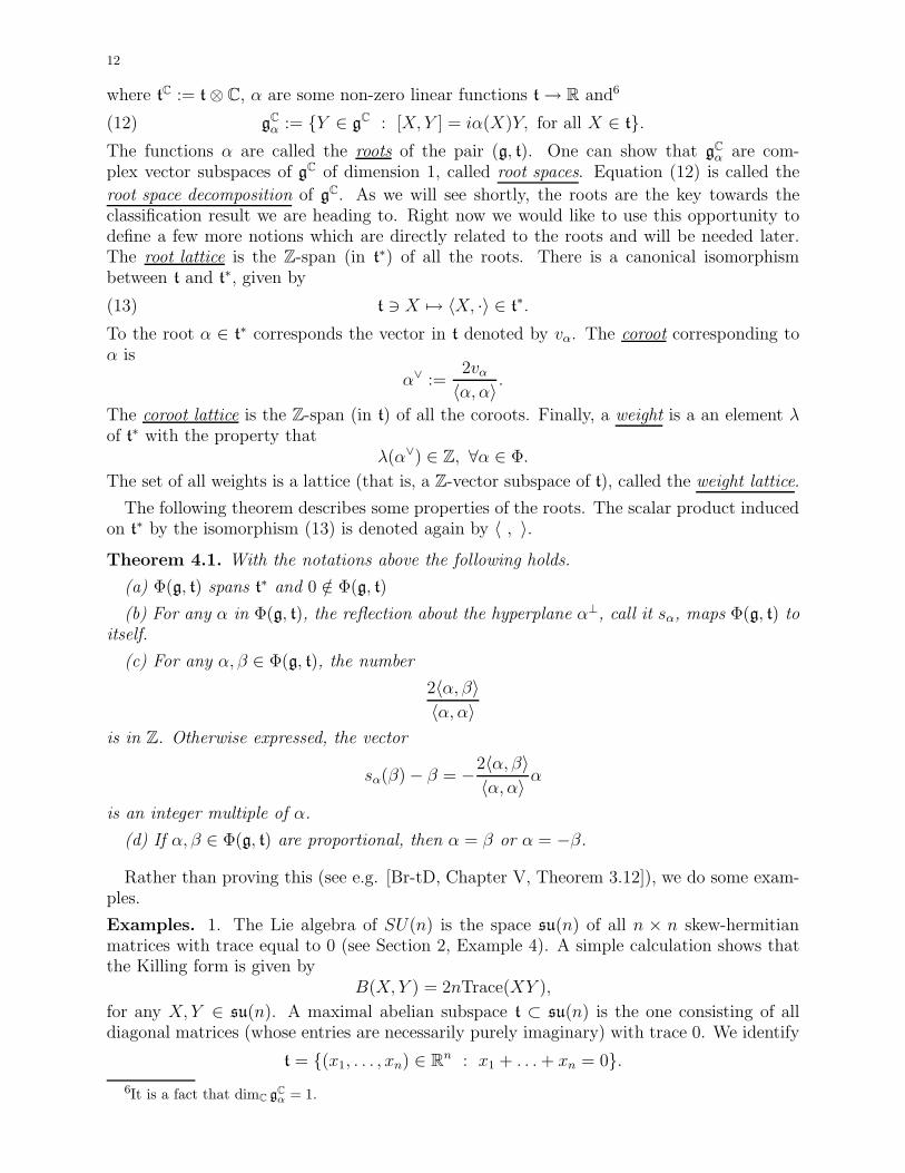
Figure 1. The roots of su(2): we identify t∗ with the2-plane t = (x1, x2, x3) ∈ R3 : x1 + x2 + x3 = 0. Thesix continuous arrows are the roots and the two dottedarrows span the weight lattice.

2. The Lie algebra of SO(n) (see Example 6, Section 2) is the space so(n) of all skew-symmetric n × n matrices with real entries and trace 0 (prove this!). Its complexification

so(n, C) := so(n) ⊗ C

consists of all skew-symmetric n × n matrices with complex entries and trace 0. There isa difference between the cases n even and n odd, due to the form of the elements of themaximal abelian subalgebra. To give the students a rough idea about this, we only mentionthat

14

• a maximal abelian subspace of so(4) consists of all matrices of the form

0 h1 0 0−h1 0 0 0

0 0 0 h2

0 0 −h2 0

where h1, h2 ∈ R

• a maximal abelian subspace of so(5) consists of all matrices of the form

0 h1 0 0 0−h1 0 0 0 0

0 0 0 h2 00 0 −h2 0 00 0 0 0 0

,

where h1, h2 ∈ R

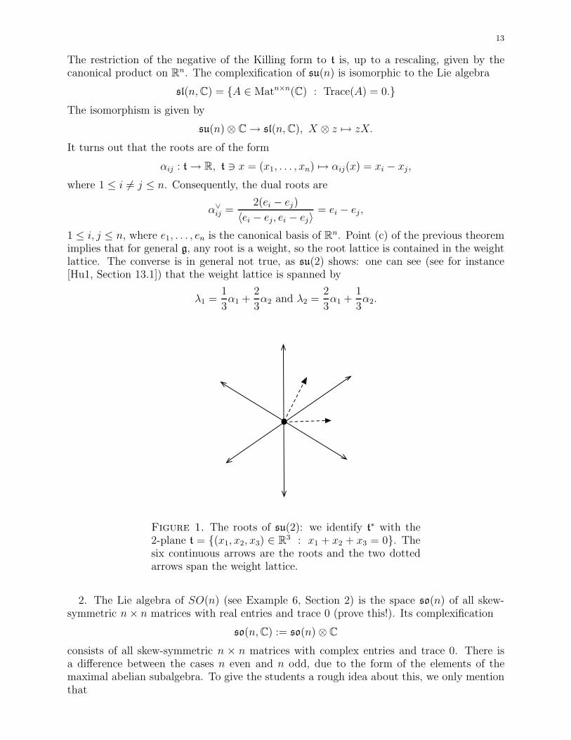
For a complete discussion of the roots, one can see [Kn, Ch. II, Section 1] or [Fu-Ha,Section 18.1]. We will confine ourselves to describe the roots and the weights for so(4, C)and so(5, C), see Figures 2 and 3).

Figure 2. The roots of so(4), which are represented bycontinuous lines. The dotted arrows span the weight lat-tice.

3. To determine the Lie algebra of Sp(n), call it sp(n), we use the description given inExample 7, Section 2, eq. (9): we deduce that sp(n) consists of all X ∈ u(2n) (that is,skew-hermitean 2n × 2n matrices) with

X = JXJ−1.

The set of all 2n× 2n matrices which satisfy only the last condition is denoted by7 sp(n, C),so that we can write

sp(n) = u(2n) ∩ sp(n, C).

Otherwise expressed,

sp(n) =

(

B −CC B

)

: B, C ∈ Matn×n(C), BT = −B, CT = C.

7This notation is used for instance in [Kn] (see Chapter I, Section 8]); in [Fu-Ha], the same Lie algebra isdenoted by sp2n(C) (see Lecture 16).

15

Figure 3. The roots of so(5): it is interesting to notethat here the root and the weight lattice coincide.

The complexification of this is just sp(n, C) (this is because the complexification of u(2n)is the space of all complex 2n × 2n matrices, and sp(n, C) is a complex vector space). Amaximal abelian subalgebra of sp(n, C) is

t =

(

D 00 D

)

: D is a diagonal n × n matrix , D = −D.

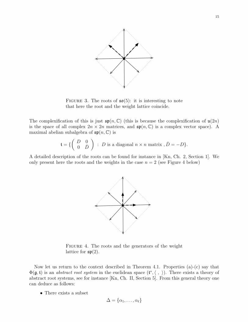
A detailed description of the roots can be found for instance in [Kn, Ch. 2, Section 1]. Weonly present here the roots and the weights in the case n = 2 (see Figure 4 below)

Figure 4. The roots and the generators of the weightlattice for sp(2).

Now let us return to the context described in Theorem 4.1. Properties (a)-(c) say thatΦ(g, t) is an abstract root system in the euclidean space (t∗, 〈 , 〉). There exists a theory ofabstract root systems, see for instance [Kn, Ch. II, Section 5]. From this general theory onecan deduce as follows:

• There exists a subset

∆ = α1, . . . , αℓ

16

of Φ(g, t) which is a linear basis of t∗ and any α ∈ Φ(g, t) can be written as

α =

ℓ∑

k=1

mkαk,

where mk ∈ Z are all in Z≥0 or all in Z≤0. Here ℓ denotes the dimension of t. Theelements of ∆ are called simple roots. The roots α for which all mk are in Z≥0 arecalled positive: the set of all those roots is denoted by Φ+.

• The group of linear transformations of8 t generated by the reflections about theplanes ker α, α ∈ Φ(g, t), is finite; this is called the Weyl group of (g, t). It is actuallygenerated by the reflections s1, . . . , sℓ about ker α1, . . . , ker αℓ.

An important result in the theory of abstract root systems gives their classification:

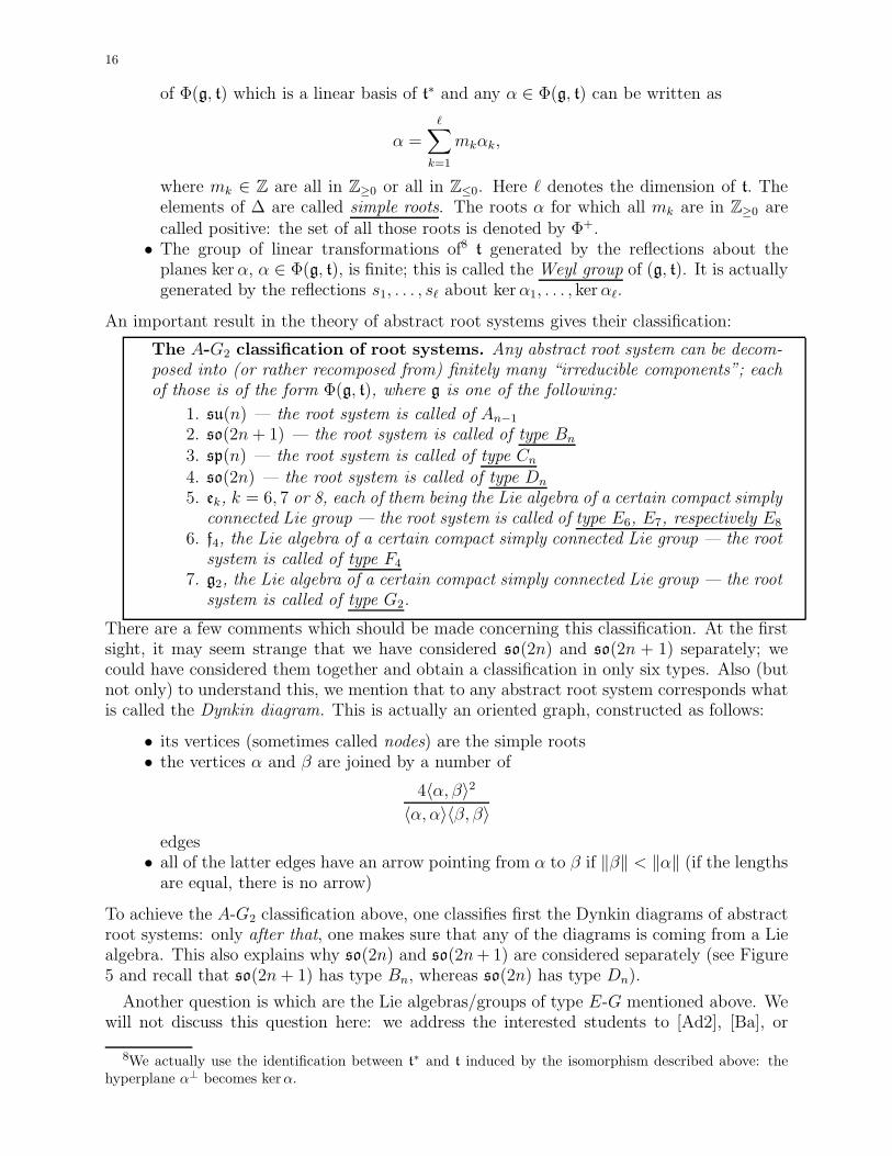
The A-G2 classification of root systems. Any abstract root system can be decom-posed into (or rather recomposed from) finitely many “irreducible components”; eachof those is of the form Φ(g, t), where g is one of the following:

1. su(n) — the root system is called of An−1

2. so(2n + 1) — the root system is called of type Bn

3. sp(n) — the root system is called of type Cn

4. so(2n) — the root system is called of type Dn

5. ek, k = 6, 7 or 8, each of them being the Lie algebra of a certain compact simplyconnected Lie group — the root system is called of type E6, E7, respectively E8

6. f4, the Lie algebra of a certain compact simply connected Lie group — the rootsystem is called of type F4

7. g2, the Lie algebra of a certain compact simply connected Lie group — the rootsystem is called of type G2.

There are a few comments which should be made concerning this classification. At the firstsight, it may seem strange that we have considered so(2n) and so(2n + 1) separately; wecould have considered them together and obtain a classification in only six types. Also (butnot only) to understand this, we mention that to any abstract root system corresponds whatis called the Dynkin diagram. This is actually an oriented graph, constructed as follows:

• its vertices (sometimes called nodes) are the simple roots• the vertices α and β are joined by a number of

4〈α, β〉2

〈α, α〉〈β, β〉

edges• all of the latter edges have an arrow pointing from α to β if ‖β‖ < ‖α‖ (if the lengths

are equal, there is no arrow)

To achieve the A-G2 classification above, one classifies first the Dynkin diagrams of abstractroot systems: only after that, one makes sure that any of the diagrams is coming from a Liealgebra. This also explains why so(2n) and so(2n + 1) are considered separately (see Figure5 and recall that so(2n + 1) has type Bn, whereas so(2n) has type Dn).

Another question is which are the Lie algebras/groups of type E-G mentioned above. Wewill not discuss this question here: we address the interested students to [Ad2], [Ba], or

8We actually use the identification between t∗ and t induced by the isomorphism described above: thehyperplane α⊥ becomes kerα.

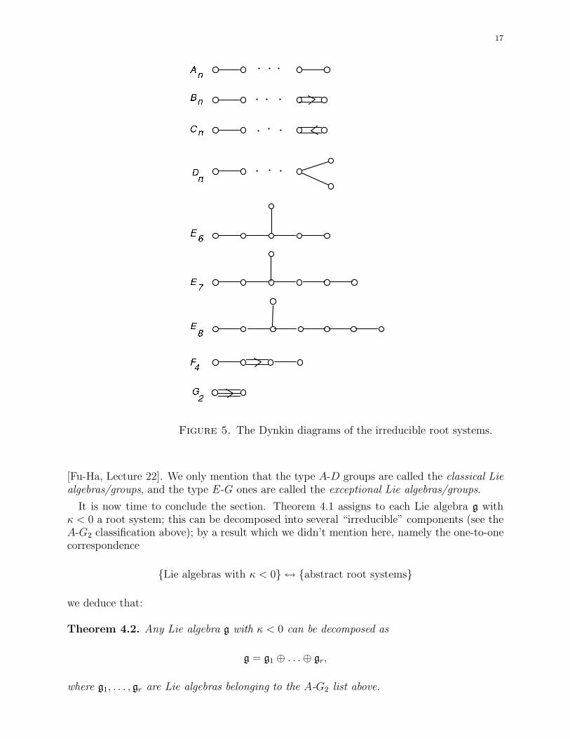
17A B C DEEEF G

nn nn6

784 2Figure 5. The Dynkin diagrams of the irreducible root systems.

[Fu-Ha, Lecture 22]. We only mention that the type A-D groups are called the classical Liealgebras/groups, and the type E-G ones are called the exceptional Lie algebras/groups.

It is now time to conclude the section. Theorem 4.1 assigns to each Lie algebra g withκ < 0 a root system; this can be decomposed into several “irreducible” components (see theA-G2 classification above); by a result which we didn’t mention here, namely the one-to-onecorrespondence

Lie algebras with κ < 0 ↔ abstract root systems

we deduce that:

Theorem 4.2. Any Lie algebra g with κ < 0 can be decomposed as

g = g1 ⊕ . . . ⊕ gr,

where g1, . . . , gr are Lie algebras belonging to the A-G2 list above.

18

5. The flag manifold of a type A-G2 Dynkin diagram with marked nodes

From Theorem 3.3 and the results stated at the end of section 3 we deduce that anycompact simply connected Lie group G can be written as

G = G1 × . . . × Gr,

where G1, . . . , Gr are compact simply connected belonging to the A-G2 list. The result atthe end of section 4 implies that any flag manifold is a product of adjoint orbits associated to(g, X0), where g is in the A-G2 list and X0 ∈ g. Consequently, we do not lose any generalityif we assume as follows:

Assumption 1. The Lie group G is connected and compact and its Lie algebra g

belongs to the A-G2 list in section 4.

More assumptions can be imposed on the element X0 of g, due to the following theorem.Recall first that t ⊂ g denotes a maximal abelian subalgebra. By Theorem 3.2 (b), thereexists a unique subgroup T ⊂ G with Lie algebra t. One can show that T is an abeliangroup (one uses the fact that exp : t → T is surjective). In fact T is isomorphic to a torus(see Example 3, Section 2). We call it a maximal torus in G (cf. [Kn, Ch. IV, Proposition4.30]).

Theorem 5.1. (a) The map exp : g → G is surjective.

(b) Any element of G is conjugate to an element of T . More precisely, for any k ∈ Gthere exists g ∈ G such that

gkg−1 ∈ T.

(c) Any Ad(G) orbit intersects t. More precisely, for any X ∈ g there exists g ∈ G suchthat

Ad(g)X ∈ t.

We will not prove the theorem. Point (b) is known as the “Maximal Torus Theorem”.Point (c) is related9 to it via (a). For a nice geometric proof of all points of the theorem,we recommend [Bu, Theorems 16.3 and 16.4] (point (c) is not explicitly proved there, butit follows immediately from the proof); another useful reference is [Du-Ko, Ch. 3, Theorem3.7.1]. It is worth trying to understand point (c) in the special case G = SU(n) (recall that t

consists of diagonal matrices with purely imaginary entries): it says that any skew-hermitianmatrix is SU(n)-diagonalizable.

Point (c) shows that we do not lose any generality if we study flag manifolds Ad(G)X0

such that

Assumption 2. The element X0 of g is actually in t.

In fact, as we will see shortly, we can refine this assumption. In Section 4 we have assignedto the pair (g, t) a root system, call it now Φ, and then the corresponding Weyl group, callit W . We recall that the latter is the group of linear transformations of t generated by thereflections sα, α ∈ Φ. Now let us consider the group

N(T ) := g ∈ G : gTg−1 ⊂ T,

that is, the normalizer of T in G. It is easy to see that for any g ∈ N(T ) we have

gtg−1 ⊂ t,

9I don’t see any obvious way to deduce (c) from (b), though.

19

and also that for any g ∈ T we have

gXg−1 = X, ∀X ∈ t.

This means that the group N(T )/T acts linearly on t. The action is effective, in the sensethat the natural map N(T )/T → GL(t) is injective.

Theorem 5.2. The subgroups W and N(T )/T of GL(t) are equal.

For a proof one can see for instance [Br-tD, Ch. V, Theorem 2.12] or [Kn, Ch. IV,Theorem 4.54].

Exercise. Show that the Weyl group of SU(n) acts on t described in Example 1, Section 4,by permuting the coordinates x1, . . . , xn. In other words, we can identify

W (su(n), t) = Sn.

Then find the element gij of N(T ) whose coset modulo T gives the reflection about the roothyperplane xi = xj in t.

The components of

t \⋃

α∈Φ

ker α

are polyhedral cones, called Weyl chambers. Pick a simple root system ∆ = α1, . . . , αℓ forΦ. Then one of the Weyl chambers is

C(∆) = X ∈ t : αj(X) < 0, j = 1, . . . , ℓ.

This is called the fundamental Weyl chamber. The planes ker αj, 1 ≤ j ≤ ℓ, which bound itare called the walls. The following result is relevant for our goals.

Theorem 5.3. The Weyl group acts simply transitively on the set of Weyl chambers. Thatis, for any Weyl chamber C there exists a unique w ∈ W such that

wC = C(∆).

Consequently, for the element X0 in Assumption 2 one can find w ∈ W such that wX0 isin the closure C(∆). On the other hand, we can write

w = nT ∈ N(T )/T,

thus

wX0 = nX0n−1

is in the adjoint orbit of X0. This shows that the next assumption is not restrictive.

Assumption 3. The element X0 of g is actually in C(∆) (the fundamental chamberC(∆) together with its walls) .

Our next goal is to understand how the diffeomorphism type of the flag manifold Ad(G)X0

changes when X0 moves inside C(∆). First we need to return to the root decomposition ofgC given by (12). This induces a similar decomposition of g itself, as follows:

(14) g = t ⊕⊕

α∈Φ+

gα,

where

gα = (gC

α ⊕ gC

−α) ∩ g = Y ∈ g : [X, [X, Y ]] = −α(X)2Y, ∀X ∈ t.

20

Proposition 5.4. Let the walls of C(∆) to which X0 belongs be ker αi1, . . . , ker αik , wherei1, . . . , ik ∈ 1, . . . , ℓ. Then we have the diffeomorphism

Ad(G)X0 ≃ G/Gi1,...,ik

where Gi1,...,ik denotes the connected closed subgroup of G of Lie algebra

t ⊕⊕

α∈Φ+(X0)

gα.

Here

(15) Φ+(X0) := α ∈ Φ+ : α(X0) = 0 = Φ+ ∩ SpanZαi1, . . . , αik.

In particular, if X0 is in C(∆) (that is, contained in no wall), then

Ad(G)X0 ≃ G/T.

Proof. We only need to show that the stabilizer of X0 is

(16) GX0= Gi1,...,ik ,

and use the homogeneous structure of Ad(G)X0 described by equation (5). To prove 16, wecheck as follows:

1. The Lie algebra of GX0is the same as the one of Gi1,...,ik

2. The group GX0is connected

and then we use Theorem 3.2 (b).

Let us start with 1. The Lie algebra of GX0is

X ∈ g : [X, X0] = 0.

Can you justify this? One can now easily see that we have

X ∈ gC : [X, X0] = 0 = tC ⊕⊕

α∈Φ,α(X0)=0

gC

α.

To obtain the Lie algebra of GX0we intersect the latter space with g and obtain the desired

description; it only remains to justify the second equation in (15) — we leave it as an exercisefor the students.

As about 2., we rely on the fact that the flag manifold Ad(G)X0 = G/GX0is simply

connected, a fact which will be proved later on (see Corollary 7.2). The long exact homotopysequence of the bundle

GX0→ G → G/GX0

implies that GX0is connected. For a more direct argument, one can see for instance [Du-Ko,

Chapter 3, Theorem 3.3.1].

The School will be concerned with the study of the flag manifolds

G/Gi1,...,ik

defined in Proposition 5.4, where G is a compact connected Lie group whose Liealgebra g is one of the seven in the A-G2 list and i1, . . . , ik are labels of certain simpleroots, that is, certain nodes of the Dynkin diagram of g.

Note. By Theorem 3.3 and Corollary 3.4, G can be any connected Lie group with Liealgebra g. We will often assume that G is the simply connected one: the benefit is describedin the following theorem (see for instance [Br-tD, Chapter V, Section 7]).

21

Theorem 5.5. Let g be in the A-G2 list and G a connected Lie group with Lie algebra g.Then the fundamental group of G is

π1(G) ≃ ker(exp : t → T ) / SpanZ(coroots).

In particular, if G is simply connected, then we have

ker(exp : t → T ) = SpanZ(coroots).

Exercise. Describe the flag manifold Fn and the Grassmannian Grk(Cn) in terms of Dynkin

digrams with marked nodes.

6. Flag manifolds as complex projective varieties

A useful observation in the study of flag manifolds is that they can be realized as complexsubmanifolds of some complex projective space. We recall that if V is a finite dimensionalcomplex vector space, then the corresponding projective space

P(V ) := ℓ : ℓ is a 1 − dimensional vector subspace of V

is a complex manifold10. One way to see this is by identifying V = Cn and constructing aholomorphic atlas on P(V ) = P(Cn). There is another way, which is more instructive for us.Namely, we note first that P(Cn) is just the grassmannian Gr1(C

n), so a flag manifold. Asnoticed in the first section, the group GLn(C) acts transitively on Gr1(C

n) and the stabilizerof Ce1 is C∗ × GLn−1(C) (the latter is naturally embedded in GLn(C)). Consequently wehave

P(V ) = P(Cn) = Gr1(Cn) = GLn(C)/(C∗ × GLn−1(C)).

The latter quotient space, regarded as a homogeneous manifold, is complex, since bothGLn(C) and C∗ × GLn−1(C) are open subspaces of Matn×n(C) ≃ Cn2

. A similar argumentshows that any of the manifolds of flags defined in Section 1 is a complex manifold. It is notclear though why are they projective complex manifolds, that is, how can we embed them(like Fn or Grk(C

n)) in some P(V ): this will be explained shortly.

Before going any further we discuss a few basic things about complex Lie groups. Firstrecall (see footnote page 6) that the space Matn×n(C) is a closed subspace of Mat2n×2n(R)via the embedding

Matn×n(C) ∋ A + iB 7→

(

A −BB A

)

.

We deduce that GLn(C) is a closed subspace (actually subgroup) of GL2n(R).

Definition 6.1. A complex Lie group is a subgroup G of some general linear group GLn(C)such that

1. G is a closed subspace of GLn(C)2. the Lie algebra of G is a complex vector subspace of Matn×n(C).

Note that condition 1 implies that G is a Lie group (because it’s closed in GL2n(R)) andalso that its Lie algebra is contained in Matn×n(C) as a real (but not necessarily complex)vector space.

Another notion we need is that of complex Lie algebra:

10By definition, this is a manifold with an atlas whose charts are of the form (U,ϕ) where U is open insome CN (same N for all charts) and for any two charts (U,ϕ), (V, ψ) the change of coordinates map ϕψ−1

is holomorphic.

22

Definition 6.2. A complex Lie algebra is a complex vector subspace of Matn×n(C) for somen ≥ 1, which is closed under the Lie bracket [ , ] given by

Matn×n(C) ∋ X, Y 7→ [X, Y ] := XY − Y X ∈ Matn×n(C).

We list here a few properties of complex Lie groups/Lie algebras:

• Any complex Lie group is a complex manifold.• If G is a complex Lie group of Lie algebra g and h ⊂ g is a complex Lie subalgebra

(that is, a complex vector subpace which is closed under the bracket [ , ]), thenthere exists a unique closed and connected subgroup H ⊂ G with Lie algebra h (His necessarily a complex Lie group, although it is worth looking again at the notefollowing Theorem 3.2). The quotient space

G/H = gH : g ∈ G

has a natural structure of a complex manifold.

The complex Lie groups corresponding to the Lie algebras g ⊗ C in examples 1, 2, 3 inSection 4 are as follows.

Examples of complex Lie groups. 1. The Lie algebra of

SL(n, C) := g ∈ GLn(C) : det(g) = 1

is sl(n, C). Thus SL(n, C) is a complex Lie group.

2. The Lie algebra of

SO(n, C) = g ∈ GLn(C) : g · gT = In

is so(n, C). Thus SO(n, C) is a complex Lie group.

3. The Lie algebra of

Sp(n, C) := g ∈ GLn(C) : g = JgJ−1.

is sp(n, C). Thus Spn(C) is a complex Lie group. We also note the obvious identity

Sp(n) = U(2n) ∩ Spn(C).

In general, whenever G is a compact Lie group, say G ⊂ GLn(R), one considers itsLie algebra g ⊂ Matn×n(R) and its complexification g ⊗ C which is a Lie subalgebra ofMatn×n(C). The complex Lie group corresponding to g ⊗ C is called the11 complexification

of G and is usually denoted by GC. The complexifications of SU(n), SO(n) and Sp(n) areSLn(C), SO(n, C), respectively Sp(n, C).

From now on in this section, G will be a compact connected Lie group of Lie algebra g inthe A-G2 list, and gC = g⊗C, GC will be their complexifications. As usually, we take t ⊂ g

a maximal abelian subalgebra, together with the corresponding root system Φ = Φ(g, t). Wealso pick a simple root system ∆ ⊂ Φ and denote by Φ+ the corresponding set of positiveroots. The space

b := tC ⊕⊕

α∈Φ+

gC

α

is a Lie subalgebra of gC.

11Of course one can ask if GC depends on the embedding G ⊂ GLn(R): the answer is “no, it doesn’t” (seee.g. [Du-Ko, p. 297]). This is not important for us, as we know exactly which are the complexifications forG of type A-D and for the other (exceptional) types, we may just say that we take an arbitrary embeddingand the corresponding complexification.

23

Exercise. Prove the previous claim. First show that

[gC

α, gC

β ] =

gC

α+β , if α + β ∈ Φ

0, if contrary.

Let B denote the (complex) connected Lie subgroup of GC whose Lie algebra is b. Wecall it a Borel subgroup. More generally, let us pick some nodes of the Dynkin diagram, sayi1, . . . , ik. Consider

p = pi1,...,ik := tC ⊕⊕

α

gC

α,

where the sum runs this time over

α ∈ Φ+⋃

(Φ− ∩ SpanZαi1 , . . . , αik).

Again one can show that p is a Lie subalgebra of of g. The corresponding Lie subgroup ofGC, call it

P = Pi1,...,ik

is called a parabolic subgroup12.

The next proposition tells us that the flag manifolds are GC/P , where P is parabolic.

Proposition 6.3. Denote P = Pi1,...,ik , p = pi1,...,ik .

(a) With the notations at the end of Section 5 we have

Gi1,...,ik ⊂ P.

The natural map

G/Gi1,...,ik → GC/P

is a diffeomorphism.

(b) The normalizer

NGC(p) := g ∈ GC : gpg−1 = p

is equal to P . Consequently the only Lie subgroup of GC with Lie algebra p is P .

(c) We have

P ∩ G = Gi1,...,ik .

In particular,

B ∩ G = T.

Proof (for P = B). Set

B′ := g ∈ GC | Adg(p) ⊂ p.

The latter is a closed subgroup of GC of Lie algebra b (Exercise: check this!)

We show that the natural map

(17) G/T ∋ gT 7→ gB′ ∈ GC/B′

is a diffeomorphism. We identify the tangent space to GC/B′ at IB′ as

TIB′GC/B′ = gC/b ≃∑

α∈Φ+

gC

α.

12It is interesting (although not useful to us) that any subgroup P of GC with B ⊂ P is automaticallyparabolic (see e.g. [Fu-Ha, Claim 23.48]).

24

Similarly, the tangent space to IT at G/T is

TIT G/T = g/t ≃∑

α∈Φ+

gα.

The differential at IT of the map (17) is

g/t → gC/b

induced by the inclusions; its kernel consists of the cosets in g/t of b∩g. Since the latter is t,the kernel is 0, thus the differential is an isomorphism (surjectivity follows from a dimensionargument). Consequently the map (17) is open, so its image is open in GC/B′. Since G iscompact, its image is closed, so (17) is surjective. Injectivity follows from the fact that

G ∩ B′ = T.

To justify the last equation, we only need to check that G ∩ B′ ⊂ T . To this end we write

b = tC + n,

where

n :=∑

α∈Φ−

gC

α.

Pick X0 ∈ t which is not in ker α, for any α ∈ Φ. This implies that

X ∈ g : [X, X0] = 0 = t.

If g is in G ∩ B′ then

Adg(X0) = Y + H,

where Y ∈ tC and H ∈ n. On the other hand, Adg(X0) is in g, which implies that Y ∈ t andH ∈ g (see eq. (14)). Since g ∩ n = 0, we deduce that

Adg(X0) ∈ t.

Due to the choice of X0, this implies that

Adg(t) ⊂ t,

which means that g ∈ NG(T ). We have to show that actually g ∈ T . Suppose it isn’t: thisimplies that

gmodT = w

which is an element of the Weyl group W = NG(T )/T , is different from the identity in thelatter group. One can show that

Adg(gC

α) = gC

wα,

for any α ∈ Φ (can you justify this?). There is a result in the theory of root systems whichsays that for any w ∈ W , w 6= 1, there exists a positive root α such that wα is a negativeroot (see e.g. [Kn, Chapter II, Section 5, Proposition 2.70]). This contradicts the fact thatAd(g)b = b.

Now since GC/B′ is diffeomorphic to G/T , the former has to be simply connected. Wededuce that B′ is connected, thus B′ = B and the proof is finished. The same argumentswork for general parabolic P .

We are now ready to accomplish the goal mentioned at the beginning of the section:

Proposition 6.4. The flag manifold GC/Pi1,...,ik is a projective manifold, in the sense thatit is a complex submanifold of some P(V ), where V is a complex vector space.

25

Proof (main ideas). Let λ ∈ t∗ be a weight with the property that

λ(α∨i ) ≥ 0, ∀1 ≤ i ≤ ℓ

λ(α∨i ) = 0 iff i ∈ i1, . . . , ik.

From the general representation theory, there exists a complex vector space V acted on byGC via complex linear automorphisms such that the action of tC on V given by

tC × V ∋ (X, v) 7→ X.v :=d

dt|0 exp(tX).v ∈ V

has the following properties13:

1. We have the “weight space” decomposition

V =⊕

µ

Vµ,

where µ are weights and Vµ = 0 unless µ ∈ λ − SpanZ≥0αi1, . . . , αiℓ.

2. dim Vλ = 1.3. gC

α.Vλ ⊂ Vλ+α, for any α ∈ Φ.4. For any α ∈ Φ− we have Vλ−α = 0 (this is a direct consequence of 1.).5. For α ∈ Φ+ we have Vλ−α = 0 if and only if λ(α∨) = 0.

The group GC acts naturally on P(V ). In the latter space we consider the point x repre-sented by Vλ (see point 2. above). We show that the GC-stabilizer of x is Pi1,...,ik. The Liealgebra of the stabilizer consists of all X ∈ gC with

X.Vλ ⊂ Vλ.

Is this hard to understand? From points 4. and 5. above we deduce that the Lie algebra ofthe stabilizer of x is p. From Proposition 6.3 (b), we deduce that the stabilizer is equal toP , so the orbit GC.x is just the flag manifold GC/P .

Example. Let V = Cn be the standard representation of SLn(C). The latter group acts

linearly also on the vector space∧k V, where k ≥ 1. It turns out that this representation

arises in the way described in the proof above (see [Fu-Ha, Section 15.2]). The SLn(C) orbit

on P(∧k V) consists of points C(v1 ∧ . . . ∧ vk), with v1, . . . , vk ∈ V. One can see that this

is a projective embedding of the Grassmannian Grk(Cn): in each k-plane V one picks a

basis v1, . . . , vk and one assigns to V the point C(v1 ∧ . . . ∧ vk). This is called the Pluckerembedding of the Grassmannian. For more details, see for instance [Fu-Ha, Section 23.3].

7. The Bruhat decomposition

Let g be a (real) Lie algebra belonging to the A-G list and a (compact) connected Liegroup G of Lie algebra g. We pick some nodes i1, . . . , ik in the Dynkin diagram and denote

P := Pi1,...,ik .

We are interested in the topology of the flag manifold GC/P . In this section we describe it asa CW complex. The idea is simple to describe: the cells are just the orbits of B, which actson GC/P by left multiplication. The main instrument is the Bruhat decomposition of GC,presented in the following theorem. We recall that the Weyl group of G is W = NG(T )/T .

13The space V is the representation of gC of highest weight λ, see for instance [Hu1, Chapter VI].

26

For each w ∈ W we pick nw ∈ NG(T ) whose coset modulo T is w. The subspace BnwB ofGC is independent of the choice of nw (because T ⊂ B); we denote

BwB := BnwB.

We also recall that W can also be regarded as a group of linear transformations of t: it isgenerated by the reflections s1, . . . , sℓ about the hyperplanes ker α1, . . . , ker αℓ which boundthe fundamental Weyl chamber. To the parabolic subgroup P = Pi1,...,ik we attach

WP := 〈si1 , . . . , sik〉

which is a subgroup of W . One can show that if w ∈ WP is of the form w = nmodT , then14

n ∈ P . Consequently, the subset BwP of GC depends only on the class of w in W/WP .

Theorem 7.1. (a) The group GC is the disjoint union

GC =⊔

w∈W

BwB.

If P is parabolic then

GC =⊔

wmodWP∈W/WP

BwP.

(b) In the disjoint union

GC/B =⊔

w∈W

BwB/B

any BwB/B is a subvariety of GC/B isomorphic to Cℓ(w). Here

ℓ(w) := minp : w is the product of p elements of s1, . . . , sℓ

is the length of w. In the disjoint union

GC/P =⊔

wmodWP∈W/WP

BwP/P

any BwP/P is a locally closed subvariety of GC/P isomorphic to Cℓ(w′), where w′ is theelement of the coset wmodWP whose length is minimal.

We will not prove the theorem (point (a) is proved for instance in [Ku, Theorem 5.1.3],[He, Ch. IX, Theorem 1.4] or [Hu2, Theorem 28.3]; for point (b), one can see [Ku, Theorem5.1.5]). Instead, we will discuss an example — see below. Point (b) says that GC/P is aCW complex, the (real) dimension of each cell being an even number. From a general resultabout the homology of CW complexes (see for instance [Br, Ch. IV, Section 10] or [Bo-Tu,Proposition 17.12]) we deduce as follows:

Corollary 7.2. Any flag manifold GC/P is simply connected. Moreover, all cohomologygroups H2k+1(GC/P ; Z) are zero (so we can have non-vanishing homology groups only ineven dimensions).

The orbit BwP/P is called a Bruhat cell. Its closure

Xw := BwP/P

14A proof goes as follows: assume w = sij; from Adn(gC

α) = gCsij

α, for any α ∈ Φ, we deduce that

Adn(pi1,...,ik) = pi1,...,ik

, thus n ∈ P .

27

is called a Schubert variety. Results in algebraic geometry imply that Xw is a closed sub-

variety15 of GC/P (recall from our Section 6 that the latter is a complex projective variety.It is also irreducible16: indeed, the B-orbit is a (locally closed) subvariety isomorphic toC

ℓ(w), thus it is irreducible (w.r.t. Zariski topology); in general, the closure of an irreducibletopological subspace is irreducible.

We will use the following general facts concerning the cohomology of algebraic varieties(the details can be found in [Fu, Section B3]).

Fact 1. If Y is a d-codimensional (possibly singular) irreducible closed subvariety of asmooth projective variety X, then we can attach to it the fundamental cohomology class

[Y ] ∈ H2d(X; Z).

Fact 2. Let X be a smooth projective variety with a filtration

X = X0 ⊃ X1 ⊃ . . . ⊃ Xs = φ,

where each Xj, 0 ≤ j ≤ s, is a closed subvariety. Assume that for each j we have

Xi \ Xi+1 =⊔

j

Uij

where Uij is a (locally closed) subvariety isomorphic to some Cn(i,j). Then the classes[Uij] are a basis of H∗(X, Z).

These two facts will be used to prove that the fundamental classes of Schubert varietiesare a basis of the cohomology group of GC/P . We first give a result which describes Xw;this is B invariant, thus a union of B-orbits (that is, cells) and the point is to say which arethose cells. For simplicity we only consider the case P = B.

Proposition 7.3. The following two statements are equivalent:

(a) BvB/B ⊂ Xw

(b) There exists simple roots αi1 , . . . , αik such that

• w = vsi1 . . . sik

• ℓ(w) = ℓ(v) + k.

If so, we denote v ≤ w. The resulting ordering on the Weyl group W is called theBruhat ordering (this is of course not a total ordering).

The “standard” proof can be found for instance in [Ku, Theorem 5.1.5] (this is actually avery abstract proof, using only the axioms of a Tits system) . For the classical flag manifoldFn, the result is proved in [Fu, Section 10.5].

Theorem 7.4. The classes [Xw], wWP ∈ W/WP , are a basis of H∗(GC/P ), which is calledthe Schubert basis.

Proof. (for P = B) Set

Xd :=⋃

ℓ(w)≤d

BwB/B.

15Here are a few more details: First, GC is an algebraic group (see [Fu-Ha, p. 374]) and P and B arealgebraic subgroups. The orbits of the B action on the algebraic variety GC/P are locally closed (see [Hu2,Proposition 8.3]). Consequently, the closures of such an orbit with respect to the Zariski and the usualtopologies are the same (see [Mu, Theorem 2.3.4]).

16An topological space is called irreducible if it cannot be written as a union of two closed proper subspaces.

28

These are a filtration of GC/P . The theorem follows from Fact 2: we can easily see that thefiltration Xd, d ≥ 0, satisfies the hypotheses in Fact 2 (we use Proposition 7.3).

In the following we will discuss in more detail an example.

Schubert varieties in the Grassmannian.17 For G = SU(n) we have GC = SLn(C),W = Sn (the symmetric group), B consists of all upper triangular matrices in SLn(C). Wetake the parabolic group

P =

(

A C0 B

)

: A ∈ GLk(C), B ∈ GLn−k(C) ∩ SLn(C).

The Grassmannian isGrk(C

n) = SLn(C)/P.

This is the same as the set of all k-planes in Cn: indeed, to any such plane V we attach the

coset of the element g of SLn(C) with the property that

V = gSpanCe1, . . . , ek.

The Bruhat cells are the B orbits of W/WP , which is embedded in Grk(Cn). Let us first

understand the latter embedding. We have

WP = Sk × Sn−k,

which is embedded in Sn via

Sk × Sn−k ∋ (µ, τ) 7→ (µ(1), . . . , µ(k), τ(1) + k, . . . , τ(n − k) + k) ∈ Sn

(exercise: try to justify this). Otherwise expressed, Sk × Sn−k consists of permutations σwith

σ(1), . . . , σ(k) ≤ k and k + 1 ≤ σ(k + 1), . . . , σ(n)

The elements of minimal length of W/WP = Sn/Sk×Sn−k (which label the Schubert varieties,see Theorem 7.1, (b)) are permutations σ ∈ Sn with the property that

σ(1) < . . . < σ(k) and σ(k + 1) < . . . < σ(n).

To each such σ we assign the k-plane

Vσ := SpanCeσ(1), . . . , eσ(k).

We have(

nk

)

such elements of Grk(Cn), to each of them corresponding a Schubert variety.

We first describe the Bruhat cell of Vσ. It is not hard to describe the elements of B.Vσ andsee (exercise) that the latter can be identified with Cd(σ), where

d(σ) = (σ(1) − 1) + (σ(2) − 2) + . . . + (σ(k) − k).

We denoteEj := SpanCe1, . . . , ej,

for 1 ≤ j ≤ n. One can show (exercise) that the Bruhat cell of Vσ is18

Ωσ := B.Vσ = U ∈ Grk(Cn) : dim(U ∩ Eσ(j)) = j, for all 1 ≤ j ≤ k.

The corresponding Schubert variety is

Ωσ = U ∈ Grk(Cn) : dim(U ∩ Eσ(j)) ≥ j, for all 1 ≤ j ≤ k.

17It is worth noticing that it was actually the Grassmannian manifold that Hermann Schubert, the founderof what is nowadays called “Schubert calculus”, investigated: he realized that problems in incidence geometrycan be solved by counting “intersection numbers” for the subspaces of Grk(Cn) which are now called afterhis name. His works were published between 1886 and 1903 (more on the history can be found for instancein [Kl]).

18The traditional notation is Ω, and not X , as above.

29

We can justify this as follows: if (Ur)r is a sequence of k-planes with limr→∞ Ur = U anddim(Ur ∩ E) = m (same for all r), then we have limr→∞(Ur ∩ E) ⊂ U ∩ E, thus

dim(U ∩ E) ≥ m.

There is a more convenient presentation of the Bruhat cells and Schubert varieties, whichwe give in what follows. The change is purely formal: we replace the data

1 < σ(1) < σ(2) < . . . < σ(k) < n

byn − k ≥ λ1 ≥ λ2 ≥ . . . ≥ λk ≥ 0

where λi are given by

0 ≤ (σ(1)−1 =: n−k−λ1) ≤ (σ(2)−2 =: n−k−λ2) ≤ . . . ≤ (σ(k)−k =: n−k−λk) ≤ n−k.

The same data can be arranges in a diagram as follows: in a rectangle of size k(height)×n−k(width) we choose λ1 boxes in the first row, λ2 boxes in the second one, ..., λk boxes in thelast one; the region inside the rectangle is a Young diagram (see Figure 6). With this newconvention, the Schubert variety is

(18) Ωλ = U ∈ Grk(Cn) : dim(U ∩ En−k−λj+j) ≥ j, for all 1 ≤ j ≤ k.λλλλλλ λ

123456 7 = 0= 0Figure 6. A Young diagram.

Let us record as follows:

Theorem 7.5. Pick an arbitrary flag

0 ⊂ E1 ⊂ . . . ⊂ En = Cn

where dim Ek = k, 1 ≤ k ≤ n. Then the cohomology classes [Ωλ], λ a Young diagram fittinga k × n − k box, are a basis of H∗(Gk(C

n); Z). Here Ωλ is described by equation (18).

It should be explained why did we start with an arbitrary flag E•, rather than the standardone, like in the previous discussion. The reason is that the cohomology class [Ωλ] does notdepend on the choice of E•, even though the variety Ωλ does depend on it: if necessary, wewill even use the notation Ωλ(E•).

As you know, the cohomology H∗(Grk(Cn); Z) has a ring structure (roughly, the product

of two classes [Ωλ] and [Ωµ] is “equal” to the class of the suvbariety Ωλ ∩ Ωµ). The mainproblem we will deal with in this context is:

30

The Littlewood-Richardson Problem. Find combinatorial formulae for the structureconstants of the ring H∗(Grk(C

n)) with respect to the Schubert basis. In other words, deter-mine the numbers cν

λµ from

[Ωλ][Ωµ] =∑

ν

cνλµ[Ων ].

Solutions to this problem are known and will be presented in the class lectures. The sameproblem can be posed in the general context of GC/P (see Theorem 7.4): find the structureconstants of the ring H∗(GC/P ) with respect to the Schubert basis. This question will alsobe addressed in the class lectures, probably mostly (only?) for the case of GC/B.

References

[Ad1] J. F. Adams, Lectures on Lie Groups, The University of Chicago Press, 1969[Ad2] J. F. Adams, Lectures on Exceptional Lie Groups, The University of Chicago Press, 1996[Ba] J. C. Baez, The octonions, http://math.ucr.edu/home/baez/octonions/[Bi-Ha] S. Billey and M. Haiman, Schubert polynomials for the classical groups, J.A.M.S. 8, 1995[Br-tD] T. Brocker and T. tom Dieck, Representations of Compact Lie Groups, Springer-Verlag 1985[Bo-Tu] R. Bott and L. Tu, Differential Forms in Algebraic Topology, Springer-Verlag 1982[Br] G. Bredon, Topology and Geometry, Springer-Verlag 1993[Bu] D. Bump, Lie Groups, Springer-Verlag 2004[Du-Ko] J. J. Duistermaat and J. A. C. Kolk, Lie Groups, Springer-Verlag 2000[Fu] W. Fulton, Young Tableaux, LMS Student Texts 1999[Fu-Ha] W. Fulton and J. Harris, Representation Theory, Springer-Verlag 2004[He] S. Helgason, Differential Geometry, Lie Groups, and Symmetric Spaces, Academic Press 1978[Hu1] J. Humphreys, Introduction to Lie Algebras and Representation Theory, Springer-Verlag 1972[Hu2] J. Humphreys, Linear Algebraic Groups, Springer-Verlag 1985[Kl] S. L. Kleiman, Rigorous foundation of Schubert’s enumerative calculus, Proceedings of Symposia

in Pure Mathematics, Vol. 28, 1976[Kn] A. Knapp, Lie Groups Beyond an Introduction (2nd Edition), Birkhauser 2002[Ku] S. Kumar, Kac-Moody Groups, their Flag Varieties, and Representation Theory, BIrkhauser 2001