ESTADISTICA (2010), 62, 179, pp.c©Instituto Interamericano de Estadıstica

AN INTRODUCTION OF BAYESIAN DATAANALYSIS WITH R AND BUGS: A SIMPLE

WORKED EXAMPLE

PABLO E. VERDECoordination Center for Clinical Trials, University of Duesseldorf,

Moorenstr. 5, D-40225, Duesseldorf, GermanyPabloEmilio.Verde@uni-duesseldorf.de

ABSTRACT

This article introduces the application of R and BUGS in Bayesian data analysis,mainly the basic model set up, analyzing simulation output, model checking,dealing with missing data and with the data generating process. The presentationis written informally omitting most of the technical details and concentrating onthe use of these powerful statistical computing languages in practice.

Key words

Bayesian modeling, binary data, posterior prediction, missing data, R, BUGS.

RESUMEN

Este articulo es una introduccion al uso de R y BUGS en analisis Bayesianode datos. Principalmente, la preparecion basica del modelo, el analisis de losresultados de simulacion, el diagnostico del modelo, el modelaje de datos perdidosy del proceso de generacion de datos. La presentacion es informal donde omitimosresultados tecnicos y nos concentramos en el uso de estos poderosos lenguagesestadısticos.

Palabras clave

Modelacion Bayesiana, datos binarios, prediction a posteriori, datos faltantes, R,BUGS.

1. Introduction

Bayesian models are very attractive when we have to combine multiple sourcesof information in a coherent statistical model. That makes this approach usefulto those that have to face complexities in data analysis including: repeated data

2

structures, very large multidimensional data, multi-level data, missing data, com-plex dependent data (e.g., spatial-temporal). The aim of this paper is to give anelementary introduction to Bayesian modeling by bringing together two statisti-cal software R from the R Development Core Team (2010) and BUGS (Bayesianinference Using Gibbs Sampling) as described in Spiegelhalter, Thomas, andBest (2004).

R is an open-source and freely available statistical software implementing theS language (Becker and Chambers 1984; Becker, Chambers, and Wilks 1988;Chambers and Hastie 1992; and Chambers 1998). R provides a general languagefor data analysis supported by techniques of data management, powerful graph-ics, numerical computations, model fitting, computer simulation, and much otherfunctionality. R is highly portable and runs in different operating systems includ-ing Unix, Linux, Windows, and Mac. A great feature of R is its extensibility; thesystem has been enriched with thousands of software packages built on R makingthe system a unique platform for data analysis.

BUGS is a versatile computer language for analyzing complex statistical mod-els using Markov Chain Monte Carlo (MCMC) techniques. Starting in the late1980s the BUGS project was pioneer software development in statistics by combin-ing ideas of artificial intelligence (e.g., declarative computer language, graphicalrepresentations, automatic-proof theorems) and multidimensional computer sim-ulation techniques (e.g., Gibbs sampling and Metropolis sampling) to routinelysolve complicated Bayesian computations. BUGS has been central in applicationsof Bayesian ideas over the last 20 years, see for example Lunn, Spiegelhalter,Thomas, and Best (2009).

In this paper we show how to setup a model in BUGS, call BUGS from R with thepackage R2WinBUGS (Sturtz, Ligges, Gelman 2005) analyze simulation outputs,model checking, and dealing with missing data. The structure of the paper is asfollows. In Section 2 we present a running example that is used to illustrate anumber of ideas and computational techniques. In Section 3 we present a briefintroduction to Bayesian data analysis. Section 4 is the main part of this tutorialwhere a full example is worked out in BUGS and R. Bayesian model checking ispresented in Section 5 and handling missing data in Section 6. Finally, Section 7presents a summary with further directions in this area.

2. Running example: Real versus fake coin flips

Gelman and Nolan (2002, page 106) present an interesting example that we bor-row to illustrate a series of concepts in Bayesian data analysis. One group ofstudents is instructed to flip a coin 100 times and record results writing heads as“1” and tails as “0”. The second group is instructed to create a sequence of 100“0”s and “1”s that are intended to mimic results of flipping a coin 100 times. It iscounterintuitive that sequences of truly coin flips may produce long runs of headsand tails. Usually, people believe that these sequences should produce haphaz-ard patterns with frequent but not regular alternations between heads and tails.

3

Therefore, we may expect that students in the second group may bias resultswith this stereotype in mind. These two sequences are entered in the R consoleas follows.# Sequence 1y.true <-c(0,0,1,1,1,0,0,0,1,1,0,0,1,0,0,0,0,1,0,0,0,0,1,0,0,

0,1,0,0,0,1, 0,0,0,0,0,0,0,0,1,0,0,1,1,0,0,1,0,1,0,1,1,0,0,0,0,1,1,1,1,1,1,0,0,1,1,0,0, 0,1,0,1,0,1,1,0,0,1,0,0,1,0,0,0,1,0,0,0,0,0,0,0,1,1,1,1,1,0,0,1)

# Sequence 2y.fake <-c(0,1,0,0,0,1,0,1,0,0,1,1,0,0,0,1,0,1,0,0,1,1,1,0,1,

0,0,1,1,0,0,0,1,1,1,1,0,1,0,0,0,1,1,1,0,1,0,0,0,1,1,0,0,0,1,1,0,1,1,1,1,0,0,0,1,0,0,1,0,1,1,0,1,1,0,1,1,1,0,0,0,1,1,0,0,1,0,0,0,1,0,0,1,0,0,0,0,1,0,0)

Given that the number of trials in these sequences are fixed by design we canapply a Fisher’s test to test difference of rates between sequences> fisher.test(y.true , y.fake)

Fisher ’s Exact Test for Count Data

data: y.true and y.fakep-value = 0.2203alternative hypothesis: true odds ratio is not equal to 195 percent confidence interval:0.2335482 1.4352513

sample estimates:odds ratio0.5865073

A p-value of 0.2203 shows that we can not distinguish between head’s rates ofthese sequences. That is, apparently the students did a good job in cheating coinflips. Later on in Section 5 we will see that this is a misleading result.

Large part of our applied statistical work is made by statistical procedures like theFisher exact test. In this tutorial we move away from this procedural statisticalapproach and we state us closer to the dynamic of the data analysis where sta-tistical models are inherent provisional, after the model has been fit, one shouldlook their results and see if it makes sense. In this way Bayesian and classicalstatistical modeling are very similar in their application.

3. Background in Bayesian modeling

Bayesian data analysis is an eclectic approach to applied statistics, where Bayesianinference is used to fit models to data and classical statistical is borrowed for modelchecking and model selection. In this section we present a brief introduction tothese ideas and we point out some further references.

4

3.1 Bayesian statistical inference

Suppose that yT = (y1, y2, . . . , yn) is a vector of n observations that we are goingto use to draw inference in a particular statistical problem. Bayesian modelingstarts as classical statistics by specifying the probability distribution p(y|θ) whichdepends on the unknown quantities θT = (θ1, . . . , θk).

Bayesian statistics generalizes classical statistics by regarding θ as a realizationof a random variable instead of a fixed quantity and by introducing a prior dis-tribution p(θ). The prior distribution p(θ) encapsulates what is known about θindependently of the data y. It can be constructed by using empirical informa-tion independent of y, by subjective prior beliefs about θ or can be handled justas a component introduced by the data modeler. In any case, it is intrinsicallyprovisional, once the data y is observed the prior is updated to the posterior ofθ by using the Bayes’ theorem

p(θ|y) ∝ p(y|θ)p(θ).

The need of introducing p(θ) in statistical inference is a point of discord betweenstatisticians. In particular the issue of handling at the same level potentially sub-jective information with empirical evidence. Once the prior is specified and theposterior is calculated, Bayesian inference automatically ensure important infer-ential properties. The data enters in the posterior only through the likelihoodp(y|θ), then the sufficient principle and the strong likelihood principle are satis-fied. Because the posterior density p(θ|y) is the distribution of θ given the wholedata, then any ancillary statistic to the problem is held automatically.

From the practical point of view, the advances of the MCMC techniques and theirimplementation in statistical software have shown the success of Bayesian meth-ods in several areas of statistics, including applications of hierarchical models,handling missing data, modeling large dimensional data, and so on. In practicalterms, the advantage of learning and using Bayesian methods usually overcomethe costs of having to defend this approach.

3.2 Posterior predictions and model checking

The fact that using Bayesian inference automatically incorporates nice inferentialproperties into the model does not protect us to go very wrong in a particularapplication. For this reason, the use of techniques of model checking and modelcriticism are fundamental in Bayesian data analysis. In this way, we furthergeneralize the Bayesian paradigm by extending the posterior p(θ|y) ∝ p(y|θ)p(θ)to the full statistical model

p(θ,yrep|y) ∝ p(y|θ)p(θ)p(yrep|θ),

5

where yrep is a replicated or predicted data set of the same size and shape as theobserved data y. In a typical application, yrep is simulated from p(yrep|y) thepredictive posterior distribution of yrep, which is approximated by MCMC. Modelchecking can then be performed by direct comparison between y and yrep.

To assess model misfit particular measures of discrepancy between y and yrep

have to be defined. The general approach is to use antisymmetric discrepancyfunctions of the data and the replications of the form D(y,yrep). These discrep-ancy functions are antisymmetric in the sense that if y is swapped with yrep thenthe sing of D must be changed. The advantage of using antisymmetric discrep-ancies rather than test statistics is that the discrepancies are always compared tozero, that simplifies visual model checks as well. Examples of model checking byapplying these techniques are presented in Section 5.

The use of simulated data from a model for model checking has a long traditionin data analysis, see for example Bush and Mosteller (1955, Chapter 6). Posteriorpredictive assessment was introduced by Guttman (1967), further developmentsare given by Box (1980), applications are given by Rubin (1981), a formaliza-tion is given by Rubin (1984); West (1986) and Gelfand, Dey, and Chang (1992)also present posterior predictive approaches to model evaluation. For an excel-lent introduction to Bayesian model checking see Gelman, Carlin , Stern andRubin (2004, Chapter 6) and Gelman and Hill (2007, Chapter 24).

3.3 Bayesian p-values

A Bayesian p-value is a posterior probability under a particular modeling assump-tion. Following the strategy of using antisymmetric discrepancy functions of theform D(y,yrep), then

p-value(y) = Pr[D(y,yrep) > 0|y].

In other words a Bayesian p-value is a posterior probability that a certain antisym-metric function exceeds zero. It quantifies how much a particular model deviatesfrom some data features. These results are used in practice to understand thedeficits of a model fitted.

3.4 Missing data and data collection process

Another generalization of the Bayesian paradigm is the incorporation of the datacollection mechanism into the model. The posterior is extended from p(θ|y) top(θ, φ|y, I), where I represents the information of which data points are actuallyobserved, and φ are parameters describing the design of the data-collection andrecording process.

Including the data-structure I in the model allows easily model missing data,censor data, truncated data and so on. In general, a data-collection process is

6

“ignorable” if p(θ, φ|y, I) = p(θ|y)p(φ|I), that is if the data structure can be ig-nored. For example, randomized data collection is an example of data collectionwhich is ignorable. Clearly, by understanding “ignorability” we can build non-ignorable models for example by adding covariates which can explain the datacollection process (e.g., lack of complaint or drop-outs in clinical trials) or mod-eling a priory the dependence between θ and φ. In Section 6.1 and Section 6.2we illustrate these concepts by implementing two toy examples in R.

4. Bayesian analysis with R and BUGS

4.1 Getting started with R and BUGS

In this section we assume that you have installed the last version of R and youare able to do most of the basic actions in R, such as simple statistical analysis,loading data from different formats, build basic graphics, and so on. To followthe statistical analysis of this section you have to setup your computational en-vironment as follows.

1. Install the last version of WinBUGS (1.4.3) fromhttp://www.mrc-bsu.cam.ac.uk/bugs/winbugs/contents.shtml

and follow the instructions at the “Quick Start” section, which are self-explanatory.

2. Within the R’s console install the package R2WinBUGS and load it.> install.packages(‘‘R2WinBUGS ’’, dependencies = TRUE)> library(R2WinBUGS)

3. Setup your working directory and the WinBUGS directory, e.g.> bugsdir <- ‘‘C:/ Programs/WinBUGS14 ’’> workdir <- ‘‘C:/bayesian -examples ’’

4.2 Writing the model in BUGS language

Let us start by modeling the y.true sequence and let us assume that these valuescan be modeled with a Binomial distribution. Suppose we observe y heads outof n trials assuming trials are independent, with common unknown heads rate θ,that leads to a binomial likelihood

p(y|n, θ) =

(ny

)θy(1− θ)n−y ∝ θy(1− θ)n−y.

We consider the response rate θ to be a continuous parameter, i.e., we need to givea continuous prior distribution p(θ). To represent external evidence that some

7

response rates are more plausible than others, it is mathematical convenient touse a Beta(a, b) prior distribution for θ

p(θ) ∝ θa−1(1− θ)b−1

Combining this prior with the binomial likelihood gives a posterior distribution

p(θ|y, n) ∝ p(y|θ, n)p(θ)

∝ θy(1− θ)n−y

= θy+a−1(1− θ)n−y+b−1

∝ Beta(y + a, n− y + b).

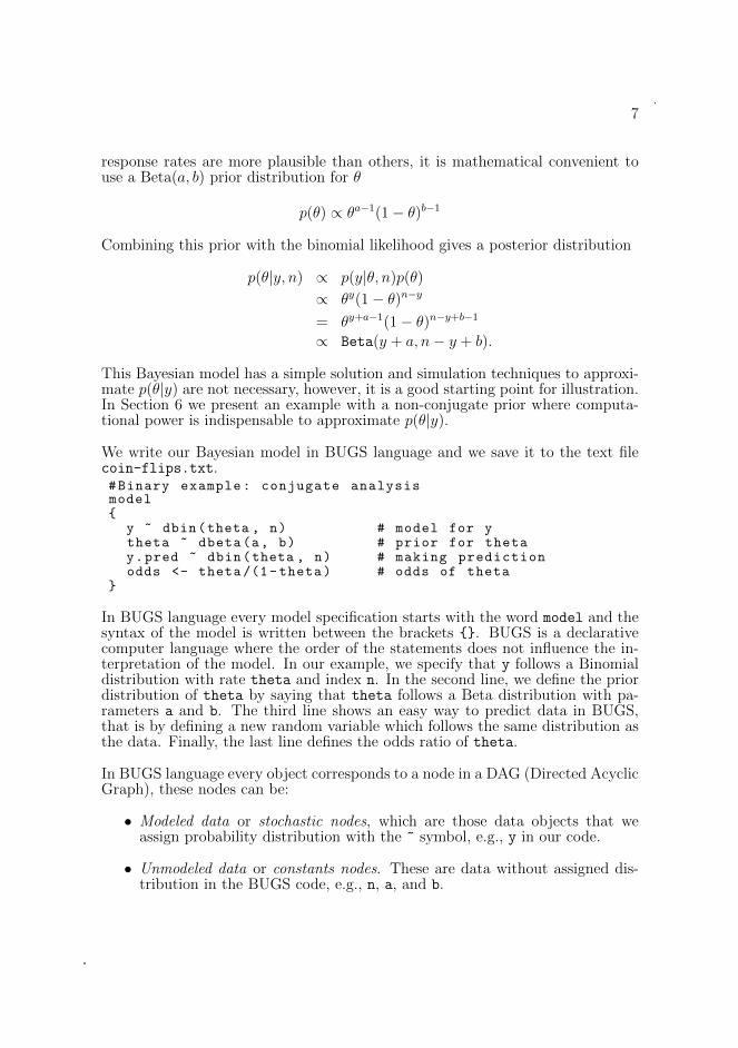
This Bayesian model has a simple solution and simulation techniques to approxi-mate p(θ|y) are not necessary, however, it is a good starting point for illustration.In Section 6 we present an example with a non-conjugate prior where computa-tional power is indispensable to approximate p(θ|y).

We write our Bayesian model in BUGS language and we save it to the text filecoin-flips.txt.#Binary example: conjugate analysismodel{

y ~ dbin(theta , n) # model for ytheta ~ dbeta(a, b) # prior for thetay.pred ~ dbin(theta , n) # making predictionodds <- theta/(1- theta) # odds of theta

}

In BUGS language every model specification starts with the word model and thesyntax of the model is written between the brackets {}. BUGS is a declarativecomputer language where the order of the statements does not influence the in-terpretation of the model. In our example, we specify that y follows a Binomialdistribution with rate theta and index n. In the second line, we define the priordistribution of theta by saying that theta follows a Beta distribution with pa-rameters a and b. The third line shows an easy way to predict data in BUGS,that is by defining a new random variable which follows the same distribution asthe data. Finally, the last line defines the odds ratio of theta.

In BUGS language every object corresponds to a node in a DAG (Directed AcyclicGraph), these nodes can be:

• Modeled data or stochastic nodes, which are those data objects that weassign probability distribution with the ~ symbol, e.g., y in our code.

• Unmodeled data or constants nodes. These are data without assigned dis-tribution in the BUGS code, e.g., n, a, and b.

8

• Parameters, these are stochastic nodes that represent unknown quantitiesin our model, e.g., theta and y.pred.

• Derived parameters or logical nodes : These are objects that are defineddeterministically using <-, in our example odds is a logical node.

• Loops or plates : These are a set of replicated model components in a forloop. For example in Section 5 we use a for loop in our model specification.

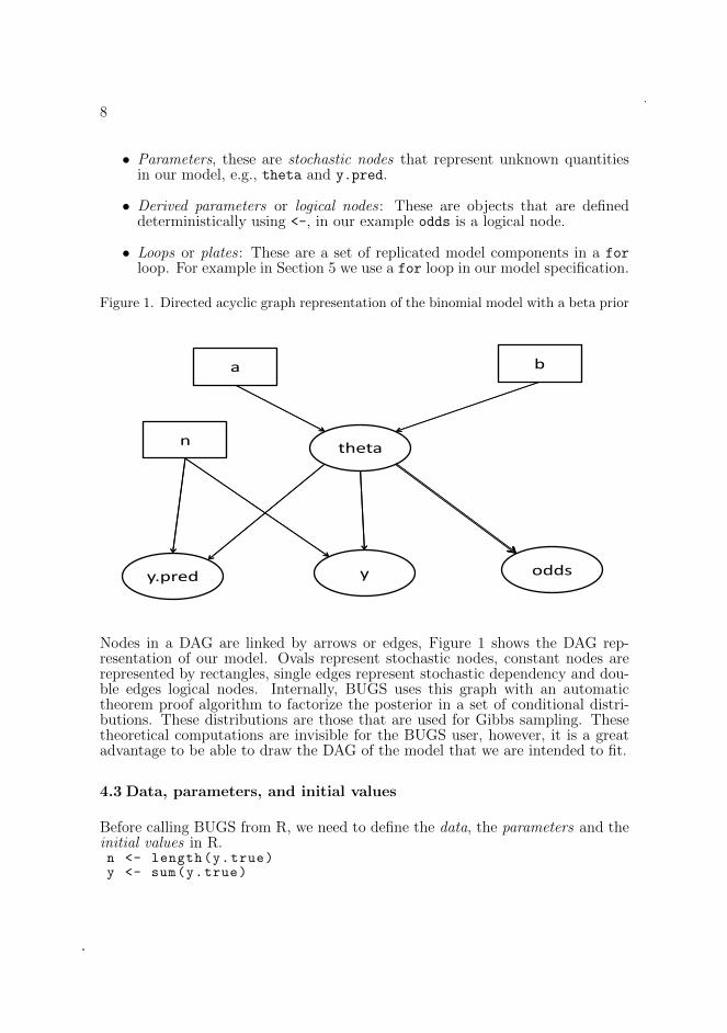
Figure 1. Directed acyclic graph representation of the binomial model with a beta prior

theta

ba

y.pred y odds

n

Nodes in a DAG are linked by arrows or edges, Figure 1 shows the DAG rep-resentation of our model. Ovals represent stochastic nodes, constant nodes arerepresented by rectangles, single edges represent stochastic dependency and dou-ble edges logical nodes. Internally, BUGS uses this graph with an automatictheorem proof algorithm to factorize the posterior in a set of conditional distri-butions. These distributions are those that are used for Gibbs sampling. Thesetheoretical computations are invisible for the BUGS user, however, it is a greatadvantage to be able to draw the DAG of the model that we are intended to fit.

4.3 Data, parameters, and initial values

Before calling BUGS from R, we need to define the data, the parameters and theinitial values in R.n <- length(y.true)y <- sum(y.true)

9

a <- 0.5b <- 0.5data1 <- list (‘‘n’’, ‘‘y’’, ‘‘a’’, ‘‘b’’)par1 <- c(‘‘theta ’’, ‘‘y.pred ’’, ‘‘odds ’’)

Here our data corresponds to the number of observations n, the number of headsin 100 flips y and the parameters of the Beta prior distribution a and b. Theunknown parameters in this analysis are the true rate theta the predictive numberof heads out of 100 in future trials y.pred and the odds of theta.

In this simple example let BUGS to use random initial values for theta andy.pred. It is, however, a good practice to take control on the initial values toavoid BUGS crashes due to numerical overflow. To work with 3 chains for eachmodel parameter we generate their initial values by combining three list() ofvalues in a single list object in R as follows.inits1 <- list(list(theta = 0.5, y.pred = 10),list(theta = 0.1, y.pred = 50),list(theta = 0.9, y.pred = 80))

This initial values are completely arbitrary and taking far away to check conver-gence issues. Alternately, we can use random generating values in R as well.

4.4 Calling BUGS from R

The function bugs() form the R2WinBUGS package is used to link R to BUGS,the value of this function is an R object that collects BUGS computations. Thefollowing runs the coin-flips.txt model in R.m1 <- bugs(data1 , inits = NULL , par1 , ‘‘coin -flips.txt ’’,

n.chains = 3, n.iter = 2000, n.thin = 1, n.burnin =floor(n.iter /2), bugs.directory = bugsdir ,working.directory = workdir , clearWD = TRUE , debug =TRUE)

In this example we use a series of options in the bugs() function by definingdifferent argument values. For example, inits=inits1 indicates the initial valuesused for computations, alternatively setting inits=NULL leaves BUGS to generaterandom initial values; n.chains=3 means that we run 3 independent chains, thiscan be used for convergence assessment; n.iter=2000 specifies the number ofiterations, n.thin=1 means that we take every simulated value, e.g., n.thin=5means that we take one every 5 values; n.burnin=floor(n.iter/2) defines thelength of the burn in period, i.e. the number of iterations that we are going todiscard, as default half of the simulating values are discard; debug=TRUE showsthe BUGS outputs on the log-file and hang up the batch in WinBUGS in a waythat we can check if BUGS syntaxes work correctly, then WinBUGS will wait forour OK to send results back to R.

We inspect the results using the function print() in R.

10

> print(m1, digits.summary = 3)

Inference for Bugs model at ‘‘coin -flips.txt ’’, fit usingWinBUGS , 3 chains , each with 4000 iterations (first2000 discarded), n.thin = 5 n.sims = 1200 iterationssaved

mean sd 2.5% 25% 50% 75% 97.5% Rhat n.efftheta 0.38 0.04 0.28 0.35 0.38 0.41 0.47 1.00 1200

y.pred 38.30 6.66 26.00 34.00 38.00 43.00 52.00 1.00 670

odds 0.62 0.12 0.40 0.54 0.62 0.70 0.88 1.00 1200

deviance 5.93 1.33 5.00 5.09 5.40 6.20 9.78 1.00 820

For each parameter , n.eff is a crude measure of effectivesample size , and Rhat is the potential scale reductionfactor (at convergence , Rhat =1).

DIC info (using the rule , pD = Dbar -Dhat)pD = 0.9 and DIC = 6.9DIC is an estimate of expected predictive error (lower

deviance is better).>

The print() output contains the following information: posterior means, stan-dard deviations and the 5 quantiles of the posterior distribution of each parameterin the model. The last two columns Rhat and n.eff are used for convergencechecking. Rhat is the ratio between a measure of variability within and betweenchains, a value of Rhat close to 1 indicates satisfactory convergence (Gelman andRubin 1992; Brooks and Gelman 1997). The n.eff refers to the effective numberof iterations adjusted by the autocorrelation between simulated values. To havea good approximation of the posteriors quantiles we need at least 2000 effectivenumber of iterations. Very low values of n.eff compared to the total number ofsimulations may indicate poor convergence induced by a drift in the simulated val-ues. The value of DIC is an estimation of the predictive error of the model and pDis an estimation of the effective number of parameters in the model (Spiegelhalter,Best, Carlin, and van der Linde 2002).

4.5 Calling BUGS from R in a Linux operating system

Although BUGS is a Windows application, it is possible to run BUGS from R inUNIX operating systems, e.g., Linux, BDS, and Mac OS X. Here we present asimple setup to run BUGS under a Linux, which can be use in other systems aswell.

1. You need to install wine a Windows emulator http://www.winehq.org/.This program makes possible to run Windows applications under Linux.

11

2. WinBUGS has to be installed under wine.

3. Clearly your working directory will have a Linux type of direction, e.g.,> workdir <- ‘‘/home/stat -lab/bayesian -examples ’’

4. To run BUGS we need to address where the executable file is located, e.g.,> bugsdir <- ‘‘/home/stat -lab/.wine/dosdevices/c:/

Programs/WinBUGS14 ’’

5. The bugs function works as usual, but you have to specify the argumentuseWINE=T.

4.6 Working with the BUGS’ results

The R object m1 generated in this analysis belong to the class bug and can befurther analyzed in R. For example, we can see the class, names, and extractvalues from this object in R.> ### obtaining results from the object ‘‘m1 ’’> class(m1)[1] ‘‘bugs ’’> names(m1)[1] ‘‘n.chains ’’ ‘‘n.iter ’’ ‘‘n.burnin ’’ ‘‘n.thin ’’...

> m1$pD[1] 0.926> m1$n.chains[1] 3

The component sims.array[] in m1 is a three dimensional array with the outputof the simulated values. The first dimension corresponds to the iterations, thesecond to chain and the third to parameters’ names. For example, to extract thefirst 10 simulated values of both parameters from chain number 1 we use:> m1$sims.array [1:10,1, ‘‘theta ’’][1] 0.3964 0.3692 0.5159 0.3611 0.3671 0.4680 0.4466

0.3351 0.3270 0.3801> m1$sims.array [1:10,1, ‘‘y.pred ’’][1] 36 31 49 42 35 45 44 35 41 38

>

These values are used to approximate the parameters’ posteriors in the model.For example, to approximate posterior percentiles of odds.theta:> odds.theta <- m1$sims.array[,,‘‘odds ’’]> quantile(odds.theta , prob=c(0.025 , 0.5, 0.975))

2.5% 50% 97.5%0.4023825 0.6222500 0.8872950>

To visualize these posteriors in R:

12

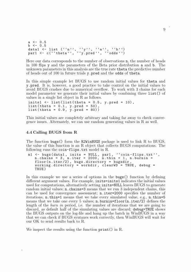
Figure 2. Results of MCMC computations. Left panel: Posterior distribution of θ rateof heads in flipping a fair coin. Right panel: Posterior of the odds θ/(1− θ)

Posterior of theta

theta.sim

Dens

ity

0.25 0.35 0.45 0.55

02

46

8

Posterior of odds theta

odds.theta

Dens

ity

0.4 0.6 0.8 1.0 1.2

0.00.5

1.01.5

2.02.5

3.0

> theta.sim <- m1$sims.array[,,‘‘theta ’’]> par(mfrow=c(1,2))> hist(theta.sim , breaks = 30, prob = TRUE ,

main=‘‘Posterior of theta ’’, col=‘‘magenta ’’)> curve(dbeta(x, shape = 0.5 + y, shape2 = 0.5 + n -y),

from = 0, to = 1, lwd=2, add = TRUE)> hist(odds.theta , breaks = 30, prob = TRUE ,

main=‘‘Posterior of odds theta ’’, col=‘‘lightblue ’’)> par(mfrow=c(1,1))

An alternative way to access m1 objects is by using the attach.bug() functionand calling the simulation arrays by the parameter names, e.g.,> attach.bugs(m1)> quantile(theta)

0% 25% 50% 75% 100%0.2147 0.3506 0.3836 0.4125 0.5245>

4.7 Checking convergence

The fact that after running a MCMC for a while we get convergence, may be atleast in theory an illusion. We need to be protected against this issue by checkingconvergence.

13

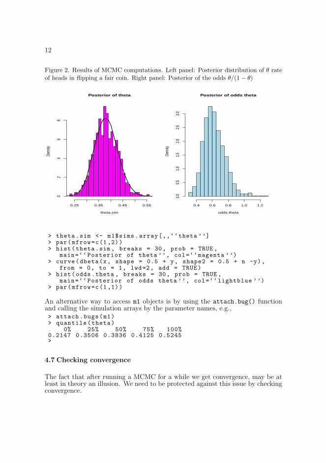
The R’s package coda (Plummer, Best, Cowles, and Vines 2010) provides a flexiblefunctionality to check convergence and visualize MCMC outputs. This function-ality includes: plots of sample traces for each parameter in each chain, kerneldensity estimates for each variable, auto-correlation and cross-correlations be-tween parameters, and plots of Gelman and Rubin diagnostic versus final iterationnumber.

To analyze the MCMC output with the coda package we need to run the bugs()function with the argument codaPkg=TRUE. The resulting object will lose the“bugs” class attribute and it will be a character class object which gives thedirection where the MCMC output files have been saved. These output files haveto be read from R and converted to a list.mcmc format. The following codeshows this process.> m1<-bugs(data1 ,+ inits=inits1 ,par1 ,‘‘coin -flips.txt ’’,n.chains = 3,+ n.iter = 4000, n.thin=5, bugs.directory = bugsdir ,+ working.directory = getwd (),+ clearWD=TRUE , debug=TRUE ,+ codaPkg=TRUE)> class(m1)[1] ‘‘character ’’> m1[1] ‘‘C:/bayesian -examples/coda1.txt ’’[2] ‘‘C:/bayesian -examples/coda2.txt ’’...> library(coda)> m1.coda <- read.bugs(m1)...Abstracting theta ... 400 valid valuesAbstracting y.pred ... 400 valid values> class(m1.coda)[1] ‘‘mcmc.list ’’>

The “m1.coda” object can be used to display MCMC convergence diagnostics, forexample we can see how these three chains are mixing and their autocorrelationfunctions with> xyplot(m1.coda)> acfplot(m1.coda)

The resulting plots are displayed in Figure 3 and Figure 4, both figures indicategood convergence in this example.

We have seen in Section 4.4 that a quick convergence check is provided by theRhat statistics, which measures the variability within and between chains, wherea value of Rhat close to 1 indicates satisfactory convergence.

14

Figure 3. Results of MCMC computations: traces for each parameter by running threeMarkov chains. These results show a clear convergence for all model parameters

iterations

510

15

0 100 200 300 400

deviance

0.40.6

0.81.0

odds

0.30.4

0.5

theta

2030

4050

60

y.pred

Figure 4. Results of MCMC computations: autocorrelation functions for each parame-ter in each chain. Different colors are used to display three chains

Lag

Autoc

orre

lation

0.0

0.2

0.4

0.6

0.8

0 5 10 15 20 25

●

●●

●

●

● ●

● ●● ●

●

●●

● ●●

●

●

●●

●●

● ●●

●

●

●●

● ●

●

●● ●

●

●●

●

●

●

● ●●

●●

●● ●

● ●●

●

●

● ● ● ●● ● ● ●

●

●

●

● ● ●●

●● ● ●

●●

●● ●

●●

deviance●

● ●

● ●●

●

●

●●

● ●

●

● ●●

●

●

● ●

●●

● ●

●

●

●

●

●●

● ● ● ●● ●

● ●

●

●●

● ● ● ●●

●●

●●

●

●

●

●

●

●●

●

● ● ● ● ●●

●

●

●

●

●

●

●●

● ●●

●●

●

●●

●

odds

●

● ●

● ●●

●

●

● ●

● ●

●

● ●●

●

●

● ●

● ●

● ●

●

●●

●

● ●

●●

●●

● ●● ●

●●

●● ● ● ●

●

●●

●●

●

●

●

●

●

●●

●

●● ● ●

●● ●

●

●

●

●

●

●

●

●●

●

●●

●

●

●

●

theta

0 5 10 15 20 25

0.0

0.2

0.4

0.6

0.8

●

●

●● ● ● ●

●● ●

●

●

●

● ●● ●

●

●

●

● ●

●●

● ●●

●

●

●● ● ●

●●

●● ● ●

●● ● ●

● ●

● ●

●

●● ●

● ●●

●

● ● ●●

● ●●

●

●● ● ●

●

●

●

●

●

●●

● ●●

●

●

● ●

y.pred

15

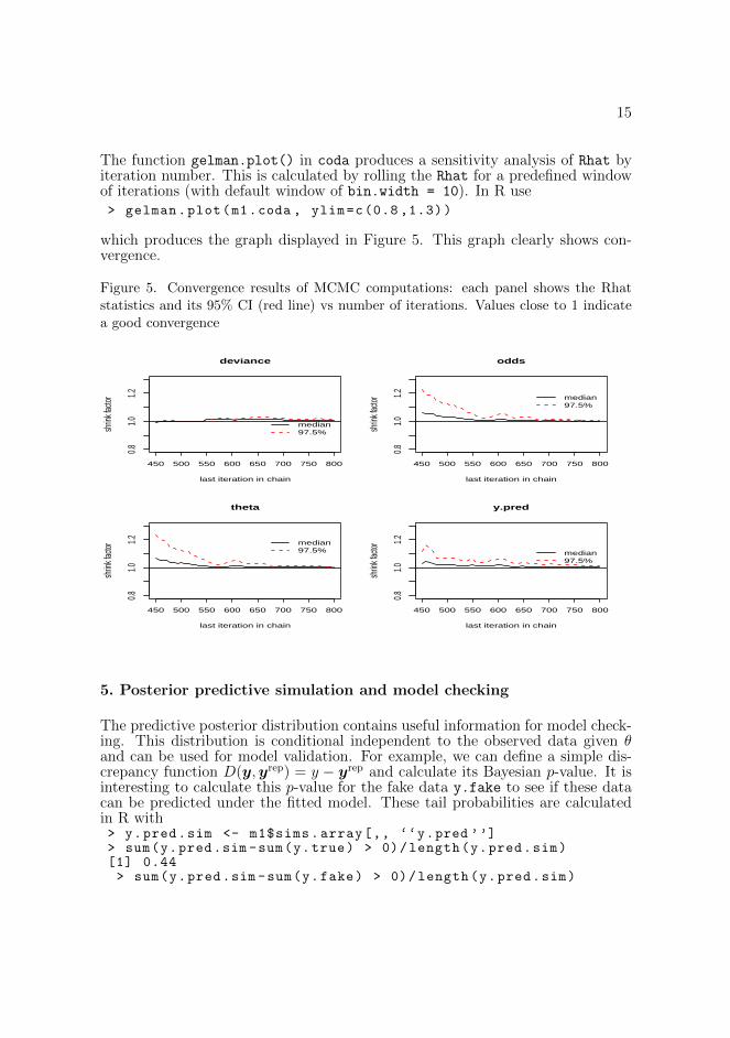
The function gelman.plot() in coda produces a sensitivity analysis of Rhat byiteration number. This is calculated by rolling the Rhat for a predefined windowof iterations (with default window of bin.width = 10). In R use> gelman.plot(m1.coda , ylim=c(0.8 ,1.3))

which produces the graph displayed in Figure 5. This graph clearly shows con-vergence.

Figure 5. Convergence results of MCMC computations: each panel shows the Rhatstatistics and its 95% CI (red line) vs number of iterations. Values close to 1 indicatea good convergence

450 500 550 600 650 700 750 800

0.81.0

1.2

last iteration in chain

shrin

k fac

tor

median97.5%

deviance

450 500 550 600 650 700 750 800

0.81.0

1.2

last iteration in chain

shrin

k fac

tor median97.5%

odds

450 500 550 600 650 700 750 800

0.81.0

1.2

last iteration in chain

shrin

k fac

tor

median97.5%

theta

450 500 550 600 650 700 750 800

0.81.0

1.2

last iteration in chain

shrin

k fac

tor

median97.5%

y.pred

5. Posterior predictive simulation and model checking

The predictive posterior distribution contains useful information for model check-ing. This distribution is conditional independent to the observed data given θand can be used for model validation. For example, we can define a simple dis-crepancy function D(y,yrep) = y − yrep and calculate its Bayesian p-value. It isinteresting to calculate this p-value for the fake data y.fake to see if these datacan be predicted under the fitted model. These tail probabilities are calculatedin R with> y.pred.sim <- m1$sims.array[,, ‘‘y.pred ’’]> sum(y.pred.sim -sum(y.true) > 0)/length(y.pred.sim)[1] 0.44> sum(y.pred.sim -sum(y.fake) > 0)/length(y.pred.sim)

16

[1] 0.141

These values show that fake data is less usual than the actual observed data.

One way to further investigate model adequacy is by defining some data featuresthat we expect from real data and assessing their discrepancy from the simulatedpredictive data.

For binary data, we define two interesting data features, one is the number ofswitches between 0’s and 1’s and the other is the length of the longest run, i.e.the longest sequence of 1’s or 0’s. The following R function calculates these twodata features.check.seq <- function(y.star){

n <- length(y.star)# number of switchesn.switch <- (n-1) - sum(y.star [1:(n-1)]==y.star [2:n])# maximum lengthL <- NULLk <- 1for(i in 2:n){

if(y.star[i-1]==y.star[i]) k <- k + 1else {L <- c(L, k)k <- 1}

}maxL <- max(L)return(c(n.switch , maxL))

}

Applying the function check.seq() to the true and fake sequences yields.> check.seq(y.fake)[1] 52 4> check.seq(y.true)[1] 43 8

Interesting, the longest run in the fake data is half of the longest run in true data.The true data has a few long sequences of 0’s and 1’s, with the longest one beinga sequence of 8 zeros. This is typical in real coin flips but counter intuitive to thestudents who emulated real data.

To quantify and visualize these discrepancy measures, we use theta.sim, thevalues sampled from θ’s posterior, and apply the check.seq() function to thepredictive values.B <- length(theta.sim)res1 <- matrix(rep(0, B*2), nrow = B, ncol = 2)for(b in 1:B){ # Simulate predictive data

y.star <- rbinom(n = 100, size = 1, prob = theta.sim[b])# Summary number of switches and longest runres1[b, ] <- check.seq(y.star)

17

}#plot for resultsplot(jitter(res1 [,2]) ~ jitter(res1 [,1]), cex =0.08,xlab = ‘‘Number of switches ’’, ylab = ‘‘Length of the

longest run ’’,main=‘‘Predictive features of flipping a fair coin 100

times ’’)

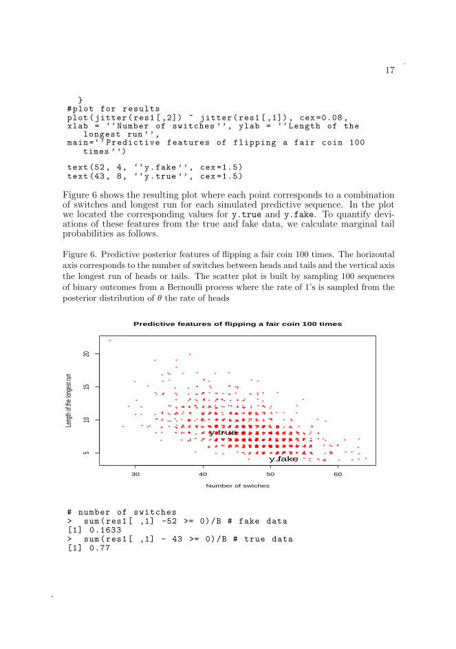
text(52, 4, ‘‘y.fake ’’, cex =1.5)text(43, 8, ‘‘y.true ’’, cex =1.5)

Figure 6 shows the resulting plot where each point corresponds to a combinationof switches and longest run for each simulated predictive sequence. In the plotwe located the corresponding values for y.true and y.fake. To quantify devi-ations of these features from the true and fake data, we calculate marginal tailprobabilities as follows.

Figure 6. Predictive posterior features of flipping a fair coin 100 times. The horizontalaxis corresponds to the number of switches between heads and tails and the vertical axisthe longest run of heads or tails. The scatter plot is built by sampling 100 sequencesof binary outcomes from a Bernoulli process where the rate of 1’s is sampled from theposterior distribution of θ the rate of heads

●

●

●

●

●

●

●

●

●

●

●

●

●●

●

●

●

●

●

●

●

●

●

●

●

●

●

●

●

●

●

●

●

●

●

●

● ●

●

●

●

●

●

●

●

●

●

●

●

●

●●

●

●

●

●

●

●

●

●

●

●

●

●

●

●

●

●

●

●

●

●

●

●

●

●

●

●

●

●

●

●

●

●

●

●

●

●

●

●

●

●

●

●

●

●

●

●

●

●

●

●

●

●

●

●

●

●

●

●

●

●

●

●

●

●

●

●

●

●

●

●

●

●

●

●

●

●

●

●

●

●

●

●

●

●

●

●

●

●

●

●

●

●

●

●

●

●

●

●

●

●

●

●

●

●

●

●

●

●

●

●

●

●●

●

●

●

●

● ●

●

●

●●

●

●

●● ●

●

●

●

●

●

●

●

●

●

●

●

●

●

●

●

●

●

●

●

●

●

●

●

●

●

●●

●

●

●

●●

●

●

●

●

●

●

●

●

●

●

●

●

●

●●

●

●

●

●

●

●

●

●

●

●

●

●

●●

●

●

●

●

●

●

●

●

●

●

●

●

●

●

●

●

●

●

●

●

●

●

●

●

●

●

● ● ●

●

●

●

●

●

●

●

●

●

●

●

●

●

●

●

●

●

●

●

●

●

●

●

●

●

●

●

●

●

●

●

●

●

●

●

●

●

●

●

●

●●

●

●

●

●

●

●●

●

●

●

●

●

●

●

●●

●●

●

●

●

●

●

●

●

●

●

●

●

●

●

●

●

●

●

●

●

●

●

●

●

●

●

●

●

●

●

●

●

●

●

●

●

●

●

●

●

●

●

●

●

●

●

●

●

●

●

●

●

●

●

●

●

●

●

●

●

●

●

●

●●

●

●

●

●

●

●

●

●

●

●

●

●

●

●

●

●

●

●

●

●

●

●

●

●

●

●

●

●

●

●

●

●

●

●●

●

●

●

●●

●

●

●

●

●

●

●

●

●

●

●

●

●

●

●

●

●

●

●

●

●

●

●

●

●

●

●

●

●

●

●

●

●

●

●

●

●

●

●

●

●

●

●

●●

●●

●

●

●

●

●

●

●

●

●

●

●

●

●

●

●

●

●

●

●

●

●

●

●

●

●

●

●

●

●

●

●

●

●

●

●

●

●

●

●

●

●

●

●

●

●

●

●● ●

●

●

●

●

●

●

●

●

●

●

●

●

●

●

●

●

●

●

●

●

●

●

●

●

●●●

●

●

●

●

●

●

●

●

●

●

●

●

●

●

●

●

●

●

●

●

●

●

●

●●

●

●

●

●

●

●

●

●

●

●

●

●

●

●

●

●

●

●

●

●

●

●

●

●

●

●

●

●

●

●

●

●

●

●

●

●

●

●

●

●

●

●

●

●

●

●

●

●

●

●

●

●

●

●

●

●

●

●

●

●

●

●

●

●

●

●

●

●

●

●

●

●

●

●

●

●●

●

●

●

●

●

●

●

●

●

●

●

●

●

●

●

●

●

●

●

●

●

●

●

●

●

●

●

●

●

●

●

● ●●

●

●

●

●

●●

●

●

●

●

● ●

●

●

●

●

●

●

●

●

●

●

●

●

●

●

●

●

●

●

●

●

●

●●

●

●

●

●

●

●

●

●

●

●

●

● ●

●

●

●

●

●

●

●

●

●●

●

●

●

●

●

●

●

●

●

●

●

●

●

●

●

●

●

●

●

●

●

●

●

●

●

●

●

●

●

●

●

●

●

●

●

●

●

●

●

●

●

●

●

●

●

●

●

●

●

●

●●●

●

●

●

●

●

●

●

●

●

●

●

●

●●

●

●

●

●

●

●

●

●

●

●

●

●●

●

●

●

●

●

●

●

●●

●

●

●

●

●

●

●● ●

●

●

●

●

●

●

●

●

●

●

●

●

●

●

●

●

●

●

●

●

● ●

●

●

●●

●

●

●

●

●

●

●

●

●●

●

●

●

●

●

●

●

●

● ●

●

●

● ●

●

●

●

●

●

●

●

●●

●

●

●

●

●

●

●

●

●

●

●

●

●

●

●

●

●

●

● ●

●

●

●

●

●

●

●

●

●

●

●

●

●

●●

●

●

●

●

●●

●

●

●

●

●

●

●

●

●

●

●

●●

●

●

●

●

●

●

●

● ●●

●

●

●

●

●

●

●

●

●

●

●

●

●

●

●●

●

●

●

●

●

●

●

●

●

●

●

●

●

●

●

●

●

●

●

●

●

●

●

●

●

●

●

●●

●

●

●

●

●

●

●

●

●

●

●

●

●

●

●

●

●

●

●

●

●

●

●

●

●

●

●●● ●

●

●

●

●

●

●●

●

●

●

●

●

●

●

●

●

●

●

●

● ●

●

●

●

●●

●

●

●

●

●

●

●

●

●

●

●

●

●

●

●

●

●

●

●

●

●

●

●

●●

●

●●

●

●●

●

●

●

●

●

●

●

●

●

●

●

●

●

●

●

●

●

●

●

●

●

●

●

●

●

●

●

●

●

●●

●

●

●

●

●

●

●

●

●

●

●

●

●

●

●

●

●

●

●

●

●

●

●

●

●

●

●

●

●

●

●

●

●

●

●

●

●

●

●

●

●

●●

●

●

●

●

●

●

●

●

●

●

●

●

●

●

●

●

●

●

●

● ●

●

30 40 50 60

510

1520

Predictive features of flipping a fair coin 100 times

Number of swiches

Leng

th of

the lo

nges

t run

y.fake

y.true

# number of switches> sum(res1[ ,1] -52 >= 0)/B # fake data[1] 0.1633> sum(res1[ ,1] - 43 >= 0)/B # true data[1] 0.77

18

>#length of the longest run> sum(res1[ ,2] - 4 <= 0)/B # fake data[1] 0.0117> sum(res1[ ,2] - 8 <= 0)/B # true data[1] 0.578

Clearly the length of the longest run presents the mayor feature deviation. Thefake data has a Bayesian tail probability of 0.0117 compared to a tail probabilityof 0.578 for the true data.

6. Missing data

6.1 Ignorable missing data mechanism

Missing data is one of the mayor issues of concern in applied data analysis. Inthis section, we present an example where the missing mechanism can be regardas ignorable. In this situation, BUGS directly imputes missing values in eachiteration by using their predictive posterior values. That is, BUGS automaticallyextends p(θ|y, I) to p(θ,ymiss|y, I) where ymiss are the set of observations withmissing data and I is an indicator vector pointing to the values that are missing.

Now, let’s generate some missing data at random in our example.# missing flipsset.seed (123)index <- sample (1:100 , 40, replace=FALSE)indexy.miss <- y.truey.miss[index] <- NA

We use this example to illustrate the application of a non-conjugate prior forθ, where the posterior cannot be handle in a close form. We transform θ byφ = logit(θ), where logit(x) = ln(x/(1 − x)), and we use for a prior of φ a t-distribution with mean equal to 0, variance equal to 1000 and with 4 degrees offreedom. In BUGS, we handle this model as follows.#Binary example: missing data analysis#Non -conjugate model with $t$ -distribution priormodel{for(i in 1:n){

y.miss[i] ~ dbern(theta) # model for y}logit(theta) <- phiphi ~ dt(mu.phi , pre.phi , 4) # prior for theta

}

The scale of θ is changed with the function logit() in BUGS, this is one ofthe few functions that can be written on the left hand side of the equation.

19

Figure 7. Directed acyclic graph representation of the binomial model with a t-distribution prior on the logistic scale. The DAG represents the loops over the observedvalues of y and over the missing values ymis. Missing data is imputed by posterior pre-dictive values

phi

pre.phimu.phi

theta

for(i in 1:n-m)

y.obs[i]

for(i in n-m+1:n)

y.miss[i]

eta

The t-distribution in BUGS uses the precision and not the variance as the scaleparameter of the distribution. Precision is defined as the inverse of the variance.BUGS uses this parametrization in all symmetric continues distributions, e.g.,Normal and double exponential.

To run this model in R, we save the BUGS code in missing-flips.txt and wechange the list of data by including the prior mean and precision of φn <- length(y.true)mu.phi <- 0pre.phi <- 0.001data1 <- list (‘‘n’’, ‘‘y.miss ’’, ‘‘mu.phi ’’, ‘‘pre.phi ’’)par1 <- c(‘‘theta ’’)

then we apply the bugs() function as usual.m.miss <- bugs(data1 , inits=NULL , par1 ,

‘‘missing -flips.txt ’’, n.chains = 3,n.iter = 4000, n.thin=5, bugs.directory =

bugsdir ,working.directory = getwd(),clearWD=TRUE , debug=TRUE)

> print(m.miss , digits.summary = 3)...

20

mean sd 2.5% 25% 50% 75% 97.5% Rhat n.efftheta 0.38 0.06 0.26 0.33 0.38 0.42 0.50 1.00 1200deviance 80.87 1.37 79.88 79.99 80.39 81.20 84.76 1.00 1200...pD = 1.0 and DIC = 81.9

The presence of missing data has been increased substantially the spread of theposterior of θ. The posterior standard deviation with complete data is 0.048compared with 0.062 with missing data. Almost a 30% of increase in variabilitydue to the missing values. Figure 8 shows the effect of imputing missing valuesin the posterior distribution of θ.

Figure 8. Posterior distribution of the heads rate θ. The histogram corresponds to theposterior distribution of θ for complete data and the solid line is the smoothed posteriorof θ with 30% of missing data. Missing data is imputed by using the predictive posteriordistribution

Comparison between posteriors

θ

Dens

ity

0.20 0.25 0.30 0.35 0.40 0.45 0.50

02

46

8

6.2 Non-ignorable missing data mechanism

Non-ignorable missing data means that the process which generates missing ob-servations is linked somehow to the data generating process. Under this assump-tion, we can improve imputation and estimation by gaining understanding on howmissing values were generated.

To illustrate the importance of including this information in the data analysis,consider the following toy example. Let θ be the head’s rate and let γ = θ/(1+θ)

21

be the rate of missing values. Now, suppose that m out of 100 flips are missing,then m/100 gives information about γ and θ as well. To implement this examplein R, we generate some missing data according to this parameters’ relationship.# Informative missing process ...> mean(y.true)

[1] 0.38> 0.38/(1+0.38)[1] 0.2753623># missing flipsset.seed (123)index <- sample (1:100 , 28, replace=FALSE)y.miss <- y.truey.miss[index] <- NAI.mis <- rep (1 ,100)I.mis[y.miss!=‘‘NA ’’] <- 0> I.mis

[1] 1 0 1 0 0 1 1 1 0 1 0 1 1 0 0

The vector I.mis has values equal to 1 for the missing data and 0 to observedvalues. This vector is used together with y.mis in BUGS as follows.#Binary example: informative missing data analysismodel{for(i in 1:n){

y.miss[i] ~ dbern(theta) # model for yI.mis[i] ~ dbern(gamma) # model for missing

indicator}gamma <- theta /(1+ theta)logit(theta) <- phiphi ~ dt(mu.phi , pre.phi , 4) # prior for theta

}

We save this model as missing-flips2.txt and we run the analysis in R.data1 <-

list(‘‘n’’,‘‘y.miss ’’,‘‘I.mis ’’,‘‘mu.phi ’’,‘‘pre.phi ’’)par1 <- c(‘‘theta ’’)m.miss2 <- bugs(data1 , inits=NULL , par1 ,

‘‘missing -flips2.txt ’’, n.chains = 3, n.iter = 4000,n.thin=5, bugs.directory = bugsdir , working.directory =getwd (), clearWD=TRUE , debug=TRUE)

> print(m.miss2 , digits.summary = 3)mean sd 2.5% 25% 50% 75% 97.5% Rhat n.eff

theta 0.3 0.04 0.2 0.3 0.3 0.3 0.4 1 1200deviance 213.6 1.2 212.9 212.9 213.2 213.9 217.3 1 1200

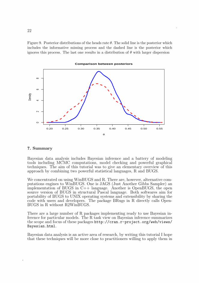
Now we can compare these results with the model ignoring the missing mechanismimplemented in the file missing-flips.txt. There is an increase of 33% ofvariability in the posterior of θ. Figure 9 compares these two posteriors.

22

Figure 9. Posterior distributions of the heads rate θ. The solid line is the posterior whichincludes the informative missing process and the dashed line is the posterior whichignores this process. The last one results in a distribution of θ with larger dispersion

0.20 0.25 0.30 0.35 0.40 0.45 0.50 0.55

02

46

8

Comparison between posteriors

θ

Dens

ity

7. Summary

Bayesian data analysis includes Bayesian inference and a battery of modelingtools including MCMC computations, model checking and powerful graphicaltechniques. The aim of this tutorial was to give an elementary overview of thisapproach by combining two powerful statistical languages, R and BUGS.

We concentrated on using WinBUGS and R. There are, however, alternative com-putations engines to WinBUGS. One is JAGS (Just Another Gibbs Sampler) animplementation of BUGS in C++ language. Another is OpenBUGS, the opensource version of BUGS in structural Pascal language. Both softwares aim forportability of BUGS to UNIX operating systems and extensibility by sharing thecode with users and developers. The package BRugs in R directly calls Open-BUGS in R without R2WinBUGS.

There are a large number of R packages implementing ready to use Bayesian in-ference for particular models. The R task view on Bayesian inference summarizesthe scope and focus of these packages http://cran.r-project.org/web/views/Bayesian.html.

Bayesian data analysis is an active area of research, by writing this tutorial I hopethat these techniques will be more close to practitioners willing to apply them in

23

their own work.

8. Acknowledgements

The author is very grateful to the Editorial Board of Estadıstica for the inviti-tation to write this tutorial paper and in particular to Veronica Beritich for herhelp and patience during the editorial process.

References

BECKER R. A. AND CHAMBERS J. M. (1984). S. An Interactive Environmentfor Data Analysis and Graphics. Wadsworth & Brooks/Cole, Pacific Grove.

BECKER R. A. CHAMBERS J. M. AND WILKS A. R. (1988). The New S.Language. Chapman & Hall, New York.

BOX G. E. P. (1980). “Sampling and Bayes inference in scientific modelling androbustness.” Journal of the Royal Statistical Society, Series A. 143: 383–430.

BROOKS S. P. AND GELMAN A. (1997). “General methods for monitoringconvergence of iterative simulations.” Journal of Computational and GraphicalStatistics. 7: 434–455.

BUSH, R. R. AND MOSTELLER, F. (1955). Stochastic Models for Learning.Wiley, New York.

CHAMBERS J. M. (1998). Programming with Data. A Guide to the S Language.Springer-Verlag, New York.

CHAMBERS J. M. AND HASTIE T. J. (1992). Statistical Models in S. Chapman& Hall, New York.

GELFAND, A. E., DEY, D. K., AND CHANG, H. (1992). “Model determinationusing predictive distributions, with implementation via sampling-based methods.”Bayesian Statistics. 4: 147–167. Oxford University Press, New York.

GELMAN A. AND HILL J. (2007). Data Analysis Using Regression and Multi-level/Hierarchical Models, 513–527. Cambridge University Press, New York.

GELMAN A. AND NOLAN D. (2002). Teaching Statistics: A Bag of Tricks.Oxford University Press, Oxford.

GELMAN A. AND RUBIN D. B. (1992). “Inference from iterative simulationusing multiple sequences (with discussion).” Statistical Science. 7: 457–511.

24

GELMAN A., CARLIN J. B., STERN H. S., AND RUBIN, D. B. (2004). BayesianData Analysis, Second Edition. Chapman & Hall, New York.

GUTTMAN, I. (1967). “The use of the concept of a future observation ingoodness-of-fit problems.” Journal of the Royal Statistical Society, Series B. 29:83–100.

LUNN D., SPIEGELHALTER D., THOMAS A., AND BEST N. (2009). “TheBUGS project: Evolution, critique and future directions.” Statistics in Medicine.28: 3049–3067.

PLUMMER M., BEST N., COWLES K., AND VINES K. (2010). “Coda: Outputanalysis and diagnostics for MCMC.” R package version 0.13–5. http://CRAN.R-project.org/package=coda.

R DEVELOPMENT CORE TEAM (2010). R: A Language and Environment forStatistical Computing. Vienna: R Foundation for Statistical Computing. ISBN3-900051-07-0. http://www.R-project.org.

RUBIN, D. B. (1981). “Estimation in parallel randomized experiments.” Journalof Educational and Behavioral Statistics. 6: 377–400.

RUBIN, D. B. (1984). “Bayesian justifiable and relevant frequency calculationsfor the applied statistician.” The Annals of Statistics. 12: 1151–1172.

SPIEGELHALTER D. J., BEST N. G., CARLIN B. P., VAN DER LINDEA. (2002). “Bayesian measures of model complexity and fit (with discussion).”Journal of the Royal Statistical Society, Series B. 64: 583–640.

SPIEGELHALTER, D. J., THOMAS A., AND BEST, N. (2004). WinBUGS,Version 1.4, Upgraded to 1.4.1, User Manual. MRC Biostatistics Unit, Cam-bridge.

STURTZ S., LIGGES U., AND GELMAN A. (2005). “R2WinBUGS: A Packagefor Running WinBUGS from R.” Journal of Statistical Software. 12: 1–16.

WEST, M. (1986). “Bayesian model monitoring.” Journal of the Royal StatisticalSociety, Series B. 48: 70–78.

Invited TutorialReceived August 2010Revised December 2010