An Interactive Environment for the Modeling

and Discovery of Scientific Knowledge

Will Bridewell a,1,∗, Javier Nicolas Sanchez a, Pat Langley a,1,

Dorrit Billman a,1

aComputational Learning Laboratory, Center for the Study of Language and

Information, Stanford University, Stanford, CA 94305 USA

Abstract

Existing tools for scientific modeling offer little support for improving models inresponse to data, whereas computational methods for scientific knowledge discoveryprovide few opportunities for user input. In this paper, we present a language forstating process models and background knowledge in terms familiar to scientists,along with an interactive environment for knowledge discovery that lets the userconstruct, edit, and visualize scientific models, use them to make predictions, andrevise them to better fit available data. We report initial studies in three domainsthat illustrate the operation of this environment and the results of a user studycarried out with domain scientists. Finally, we discuss related research on modelingformalisms and model revision, and we suggest priorities for additional research.

Key words: Scientific modeling, Interactive knowledge discovery, Model revision

1 Background and Motivation

Models play a central role in science, in that they utilize general laws or theo-ries to predict or explain behavior in specific situations. Models occur in manyguises, but the more complex the phenomena for which they account, the moreimportant that they be cast in some formal notation with an unambiguous

∗ Corresponding author. Tel: +1 (650) 494-3884. Fax: +1 (650) 494-1588.Email addresses: willb@csli.stanford.edu (Will Bridewell),

jsanchez@cs.stanford.edu (Javier Nicolas Sanchez), langley@isle.org (PatLangley), dbillman@psych.stanford.edu (Dorrit Billman).1 Also affiliated with the Institute for the Study of Learning and Expertise, 2164Staunton Court, Palo Alto, CA 94306 USA.

Preprint submitted to IJHCS 3 July 2006

interpretation. Moreover, the advent of fields like Earth science and systemsbiology, which attempt to explain the behavior of complex systems in termsof interacting components, have increased the need for computational tools toaid model construction and use.

A variety of computational modeling tools already exist, although they aretypically associated with particular fields. For example, STELLA (Richmondet al., 1987) provides a language and environment for creating quantitativemodels in terms of instantaneous and difference equations. This frameworkhas been adopted widely in the Earth science community for use in ecosys-tem models. Similarly, MATLAB (The Mathworks, Inc., 1997) offers an al-ternative formalism and environment for specifying quantitative models thatinclude instantaneous and differential equations. However, it is most popularin engineering circles that model complex artifacts like electric circuits.

Both these and other environments offer interactive tools that let users vi-sualize the structure of models, run them as simulations, and examine theirpredictions. However, they provide at most limited facilities for using availabledata to generate or improve models. That is, current modeling environmentsare concerned primarily with the formulation and simulation of models, notwith their discovery. However, as data become more available and as the com-plexity of models grows, scientists would increasingly stand to benefit fromsuch computational assistance.

On another front, there has been considerable research on computationalmethods for discovering knowledge from data. Much of this work, especiallywithin the data mining paradigm (e.g., Fayyad et al., 1996), has emphasizedformalisms like decision trees and logical rules that came originally from thefield of artificial intelligence. These notations are perfectly appropriate forbusiness applications, since the corporate world lacks established ways to rep-resent domain knowledge, but they are more poorly suited for scientific disci-plines, which have a long history of formalisms for encoding knowledge.

Fortunately, an alternative paradigm, known as computational scientific dis-

covery (e.g., Langley, 2000), has dealt instead with discovery of knowledgecast as numeric equations and other notations widely used in fields of sci-ence and engineering. Yet research in this framework shares with data miningan emphasis on automating the discovery process, so that, with few excep-tions, the developed methods provide little support for interaction with humanusers. Another drawback is that these methods typically focus on discoveringknowledge from scratch, and thus takes no advantage of scientists’ existingknowledge about a domain.

Clearly, scientists would benefit from computational tools that combine theadvantages of available modeling environments with the strengths of existing

2

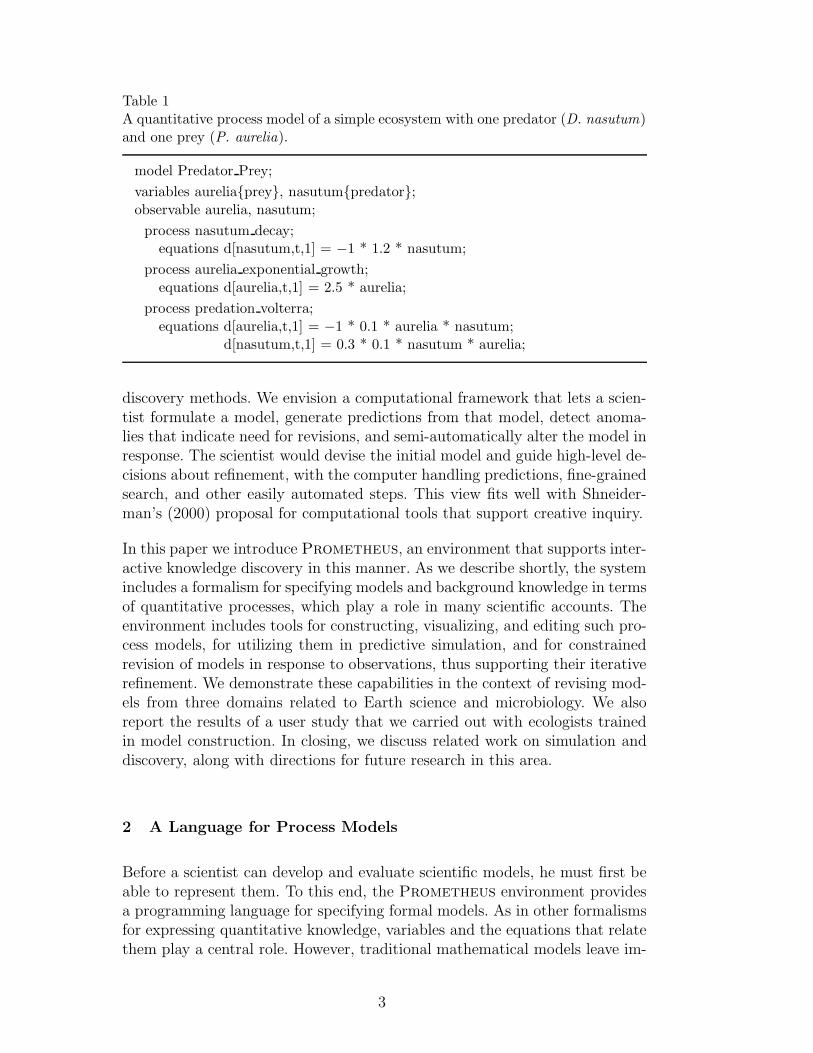
Table 1A quantitative process model of a simple ecosystem with one predator (D. nasutum)and one prey (P. aurelia).

model Predator Prey;

variables aurelia{prey}, nasutum{predator};observable aurelia, nasutum;

process nasutum decay;equations d[nasutum,t,1] = −1 * 1.2 * nasutum;

process aurelia exponential growth;equations d[aurelia,t,1] = 2.5 * aurelia;

process predation volterra;equations d[aurelia,t,1] = −1 * 0.1 * aurelia * nasutum;

d[nasutum,t,1] = 0.3 * 0.1 * nasutum * aurelia;

discovery methods. We envision a computational framework that lets a scien-tist formulate a model, generate predictions from that model, detect anoma-lies that indicate need for revisions, and semi-automatically alter the model inresponse. The scientist would devise the initial model and guide high-level de-cisions about refinement, with the computer handling predictions, fine-grainedsearch, and other easily automated steps. This view fits well with Shneider-man’s (2000) proposal for computational tools that support creative inquiry.

In this paper we introduce Prometheus, an environment that supports inter-active knowledge discovery in this manner. As we describe shortly, the systemincludes a formalism for specifying models and background knowledge in termsof quantitative processes, which play a role in many scientific accounts. Theenvironment includes tools for constructing, visualizing, and editing such pro-cess models, for utilizing them in predictive simulation, and for constrainedrevision of models in response to observations, thus supporting their iterativerefinement. We demonstrate these capabilities in the context of revising mod-els from three domains related to Earth science and microbiology. We alsoreport the results of a user study that we carried out with ecologists trainedin model construction. In closing, we discuss related work on simulation anddiscovery, along with directions for future research in this area.

2 A Language for Process Models

Before a scientist can develop and evaluate scientific models, he must first beable to represent them. To this end, the Prometheus environment providesa programming language for specifying formal models. As in other formalismsfor expressing quantitative knowledge, variables and the equations that relatethem play a central role. However, traditional mathematical models leave im-

3

plicit an important aspect of scientific knowledge—processes—whereas Pro-

metheus makes it an explicit part of its models. In fact, the notion of aprocess is the central organizing principle in the programming language, sowe refer to programs written in this formalism as process models.

We borrow this distinctive characteristic from work in qualitative process the-ory (Forbus, 1984), in which a user describes a dynamic system by the generalrelationships among its parts. That representation was designed to supportcommonsense reasoning and knowledge, whereas we developed Prometheus’language with deterministic scientific modeling in mind. Some work in quali-tative process theory includes support for quantitative knowledge (Forbus andFalkenhainer, 1990), which brings this work closer to our own, but the empha-sis still rests on the qualitative processes, with the quantitative informationstored in a separate library. Since we built Prometheus as a tool for devel-oping mathematical models, the associated language places the quantitativeinformation on equal grounds with the qualitative content.

To illustrate the use of process models, we appeal to a classic example ofpredator–prey interaction. Consider an ecosystem consisting of two protistspecies Paramecium aurelia and Didinium nasutum, wherein the latter preysupon the former. Jost and Ellner (2000) give a thorough analysis of this simpleecosystem using traditional modeling methods. We developed a model of thisecosystem on the same general model structure that guided their exploration,and we use this model to illustrate the process modeling formalism and todemonstrate the Prometheus environment.

Table 1 shows the candidate process model for the protist ecosystem. Thespecification begins with the model name (here, Predator Prey) and the vari-ables it references. This model has two variables, aurelia and nasutum, thatrepresent the population density of each species in the ecosystem. A type, usedprimarily during model revision, follows the variable’s name. In this example,aurelia has the type prey and nasutum has the type predator. The model alsodeclares both aurelia and nasutum to be observable, which means that theywere measured at some point during system activity.

Following the variable definitions come descriptions of the model’s processes.Here we have three processes that explain how the values of variables changeover time. A process consists of a name (e.g., predation volterra) and one ormore equations, plus an optional set of conditions. The processes in Table 1involve differential equations, although we will see examples of algebraic equa-tions later in the paper. The processes in this model always apply, so they haveno conditions to restrict their activity.

The first process, nasutum decay, indicates the death of D. nasutum, in whichthe left-hand side of the equation specifies a first-order differential equa-

4

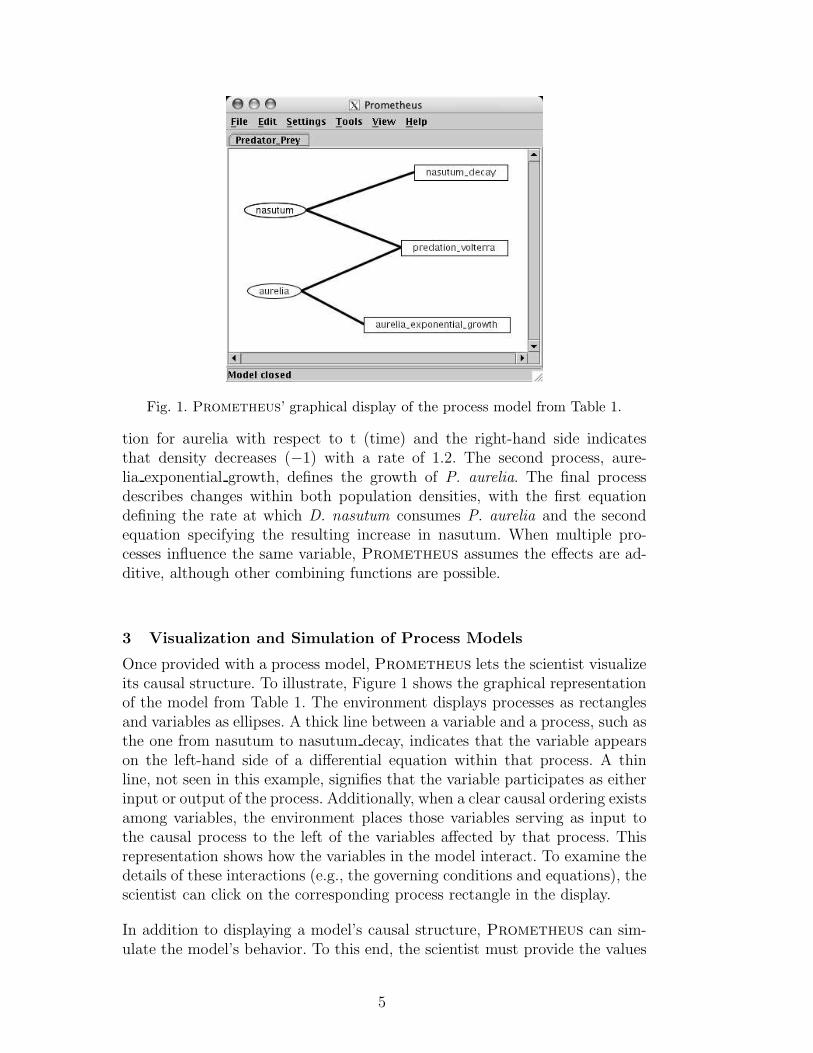
Fig. 1. Prometheus’ graphical display of the process model from Table 1.

tion for aurelia with respect to t (time) and the right-hand side indicatesthat density decreases (−1) with a rate of 1.2. The second process, aure-lia exponential growth, defines the growth of P. aurelia. The final processdescribes changes within both population densities, with the first equationdefining the rate at which D. nasutum consumes P. aurelia and the secondequation specifying the resulting increase in nasutum. When multiple pro-cesses influence the same variable, Prometheus assumes the effects are ad-ditive, although other combining functions are possible.

3 Visualization and Simulation of Process Models

Once provided with a process model, Prometheus lets the scientist visualizeits causal structure. To illustrate, Figure 1 shows the graphical representationof the model from Table 1. The environment displays processes as rectanglesand variables as ellipses. A thick line between a variable and a process, such asthe one from nasutum to nasutum decay, indicates that the variable appearson the left-hand side of a differential equation within that process. A thinline, not seen in this example, signifies that the variable participates as eitherinput or output of the process. Additionally, when a clear causal ordering existsamong variables, the environment places those variables serving as input tothe causal process to the left of the variables affected by that process. Thisrepresentation shows how the variables in the model interact. To examine thedetails of these interactions (e.g., the governing conditions and equations), thescientist can click on the corresponding process rectangle in the display.

In addition to displaying a model’s causal structure, Prometheus can sim-ulate the model’s behavior. To this end, the scientist must provide the values

5

Fig. 2. Simulated trajectories for the predator–prey model from Table 1.

for each exogenous variable (i.e., those input variables that the model shouldnot explain), initial values for each variable that occurs in the left-hand sideof a differential equation, the start and end times of the simulation, and thesize of the time step. In one such run, we used initial values from Jost andEllner’s (2000) analysis, 2 setting aurelia and nasutum to 276.60 and 64.67 in-dividuals/mL, respectively. We also told the program to start the simulationon day 10, to end on day 35, and to report values once every 12 hours so thatthe timing of the predictions and the observed data would correspond.

After running the simulation, the user can view how a variable’s predictedvalues change over time, as shown in Figure 2. Prometheus draws a graphfor the variable, with the x axis representing time and the y axis representingthe variable’s value. As the results indicate, the model produces a series ofsharp peaks such that the growth of D. nasutum occurs slightly after thegrowth of P. aurelia. Once the prey population reaches its peak, a sharp declineprecedes a similar decline in the predator population. To further evaluate amodel, the user can plot the simulated results against the observed data. Forexample, Figure 3 shows how the process model’s behavior compares to thedata from Jost and Ellner’s analysis. For both species the model producesfewer and sharper peaks than were observed, with the peaks being slightlyout of synchronization with the observations.

Since the model fails to adequately reproduce the behavior of the ecosystem,the scientist may want to revise it. To this end, the graphical environmentsupports the addition and alteration of both variables and processes, 3 andthe user has full access to the underlying text of the model. Thus the scientistcan adjust the model, view the new causal structure, and simulate the newmodel’s behavior. Used in this manner, Prometheus acts primarily as atool for model visualization and simulation, but it can also serve as an active

2 These data are available at http://www.pubs.royalsoc.ac.uk/ as an appendix toJost and Ellner’s article. For this example, we used the data from their Figure 1(a)starting at day 10.3 The user can either instantiate a generic process from the library or create a newprocess from scratch.

6

Fig. 3. Simulated versus observed output for the protist ecosystem.

assistant in the analysis of data as we will illustrate in the next section.

4 Revision of Process Models

When a model’s predictions disagree with the observations, the Prometheus

user can also invoke a module for automated model revision. We can charac-terize the behavior of this system component as:

• Given: trajectories for a set of continuous variables over time;

• Given: background knowledge cast in terms of generic processes and variabletype hierarchies;

• Given: observable and theoretical variables to be modeled;

• Given: an initial model, processes that may be removed from the model orhave their parameters changed, generic processes that may be added tothe model, and constraints on model size;

• Find : a set of process models, ranked by their fit to the data, that explainthe observed trajectories.

In this section, we discuss the input to this approach in more detail, describethe search algorithm that produces the revised models, and show the outputfrom the module.

Before Prometheus can aid in model revision, it must have some knowl-edge about the domain. One type of knowledge takes the form of genericprocesses, which serve as building blocks when adding new processes to themodel. Generic processes specify the form of a model’s instantiated processesand have an analogous representation. Table 2 shows five generic processesrelevant to modeling predator–prey interaction. Each generic process consistsof five components: a name, a set of variables, a set of parameters, a set of

7

Table 2Some generic processes relevant to the predator–prey model in Table 1.

generic process logistic growth;variables S{prey};parameters p[0,3], k[0,1];equations d[S,t,1] = p * S * (1 − k * S);

generic process predation volterra;variables S1{prey}, S2{predator};parameters a[0,1], b[0,1];equations d[S1,t,1] = −1 * a * S1 * S2;

d[S2,t,1] = b * a * S1 * S2;

generic process predation holling;variables S1{prey}, S2{predator};parameters a[0,1], b[0,1], c[0,1];equations d[S1,t,1] = −1 * a * S1 * S2/(1 + c * a * S1);

d[S2,t,1] = b * a * S1 * S2 / (1 + c * a * S1);

generic process exponential growth;variables S{prey};parameters b[0,3];equations d[S,t,1] = b * S;

generic process exponential decay;variables S{species};parameters a[0,2];equations d[S,t,1] = −1 * a * S;

conditions, and a set of equation forms. Of these components, the parametersand conditions are optional. To instantiate a generic process, the user mustprovide both variables of the correct type and parameters that fall within aspecified range. For example, aurelia exponential growth in Table 1 instanti-ates exponential growth so that aurelia fills the role of S and b equals 2.5.

In addition to generic processes, the scientist must provide a type hierarchyover the variables. The types predator and prey from the protist ecosystemmodel are subtypes of species, which in turn is a subtype of number—the rootof the hierarchy. When instantiating a generic process, Prometheus mustselect variables of the appropriate types. Consider exponential decay, whichexpects a species variable. Since both aurelia and nasutum are instances ofspecies, either one can fill the role. In contrast, predation volterra requires onevariable each of the more specific types predator and prey. Here, knowledge ofthe variable types keeps Prometheus from considering implausible modelsin which predator and prey switch roles.

Along with this general domain knowledge, the scientist provides Prome-

theus with additional, task-specific information to direct its search for alter-native models. This information includes a set of variables to include in the

8

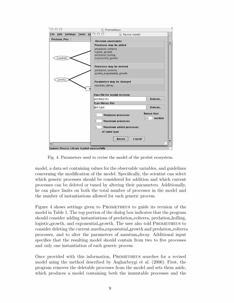
Fig. 4. Parameters used to revise the model of the protist ecosystem.

model, a data set containing values for the observable variables, and guidelinesconcerning the modification of the model. Specifically, the scientist can selectwhich generic processes should be considered for addition and which currentprocesses can be deleted or tuned by altering their parameters. Additionally,he can place limits on both the total number of processes in the model andthe number of instantiations allowed for each generic process.

Figure 4 shows settings given to Prometheus to guide its revision of themodel in Table 1. The top portion of the dialog box indicates that the programshould consider adding instantiations of predation volterra, predation holling,logistic growth, and exponential growth. The user also told Prometheus toconsider deleting the current aurelia exponential growth and predation volterraprocesses, and to alter the parameters of nasutum decay. Additional inputspecifies that the resulting model should contain from two to five processesand only one instantiation of each generic process.

Once provided with this information, Prometheus searches for a revisedmodel using the method described by Asgharbeygi et al. (2006). First, theprogram removes the deletable processes from the model and sets them aside,which produces a model containing both the immutable processes and the

9

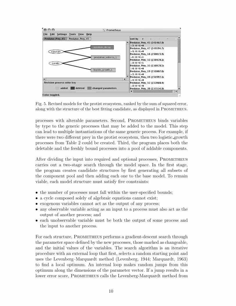
Fig. 5. Revised models for the protist ecosystem, ranked by the sum of squared error,along with the structure of the best fitting candidate, as displayed in Prometheus.

processes with alterable parameters. Second, Prometheus binds variablesby type to the generic processes that may be added to the model. This stepcan lead to multiple instantiations of the same generic process. For example, ifthere were two different prey in the protist ecosystem, then two logistic growthprocesses from Table 2 could be created. Third, the program places both thedeletable and the freshly bound processes into a pool of addable components.

After dividing the input into required and optional processes, Prometheus

carries out a two-stage search through the model space. In the first stage,the program creates candidate structures by first generating all subsets ofthe component pool and then adding each one to the base model. To remainviable, each model structure must satisfy five constraints:

• the number of processes must fall within the user-specified bounds;• a cycle composed solely of algebraic equations cannot exist;• exogenous variables cannot act as the output of any process;• any observable variable acting as an input to a process must also act as the

output of another process; and• each unobservable variable must be both the output of some process and

the input to another process.

For each structure, Prometheus performs a gradient-descent search throughthe parameter space defined by the new processes, those marked as changeable,and the initial values of the variables. The search algorithm is an iterativeprocedure with an external loop that first, selects a random starting point anduses the Levenberg–Marquardt method (Levenberg, 1944; Marquardt, 1963)to find a local optimum. An internal loop makes random jumps from thisoptimum along the dimensions of the parameter vector. If a jump results in alower error score, Prometheus calls the Levenberg-Marquardt method from

10

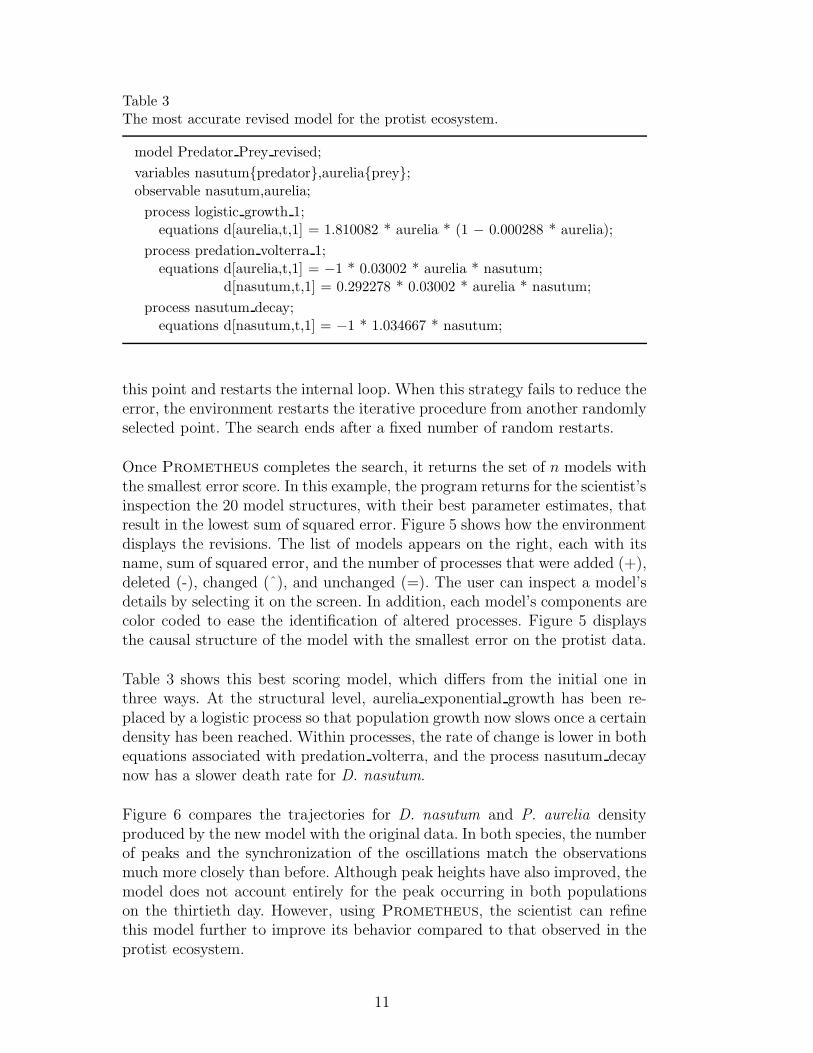
Table 3The most accurate revised model for the protist ecosystem.

model Predator Prey revised;

variables nasutum{predator},aurelia{prey};observable nasutum,aurelia;

process logistic growth 1;equations d[aurelia,t,1] = 1.810082 * aurelia * (1 − 0.000288 * aurelia);

process predation volterra 1;equations d[aurelia,t,1] = −1 * 0.03002 * aurelia * nasutum;

d[nasutum,t,1] = 0.292278 * 0.03002 * aurelia * nasutum;

process nasutum decay;equations d[nasutum,t,1] = −1 * 1.034667 * nasutum;

this point and restarts the internal loop. When this strategy fails to reduce theerror, the environment restarts the iterative procedure from another randomlyselected point. The search ends after a fixed number of random restarts.

Once Prometheus completes the search, it returns the set of n models withthe smallest error score. In this example, the program returns for the scientist’sinspection the 20 model structures, with their best parameter estimates, thatresult in the lowest sum of squared error. Figure 5 shows how the environmentdisplays the revisions. The list of models appears on the right, each with itsname, sum of squared error, and the number of processes that were added (+),deleted (-), changed (ˆ), and unchanged (=). The user can inspect a model’sdetails by selecting it on the screen. In addition, each model’s components arecolor coded to ease the identification of altered processes. Figure 5 displaysthe causal structure of the model with the smallest error on the protist data.

Table 3 shows this best scoring model, which differs from the initial one inthree ways. At the structural level, aurelia exponential growth has been re-placed by a logistic process so that population growth now slows once a certaindensity has been reached. Within processes, the rate of change is lower in bothequations associated with predation volterra, and the process nasutum decaynow has a slower death rate for D. nasutum.

Figure 6 compares the trajectories for D. nasutum and P. aurelia densityproduced by the new model with the original data. In both species, the numberof peaks and the synchronization of the oscillations match the observationsmuch more closely than before. Although peak heights have also improved, themodel does not account entirely for the peak occurring in both populationson the thirtieth day. However, using Prometheus, the scientist can refinethis model further to improve its behavior compared to that observed in theprotist ecosystem.

11

Fig. 6. Simulated trajectories predicted by the revised protist model and observedvalues for the same system.

5 Modeling an Aquatic Ecosystem Using Prometheus

In evaluating Prometheus, we have also modeled the Ross Sea ecosystem,which Arrigo et al. (2003) have described at length. For this system, scien-tists are particularly interested in the change in phytoplankton populationthroughout the year. Suspected influences include the availability of nutrientsand light, as well as grazing behavior by zooplankton. Table 4 shows an initialprocess model for this ecosystem.

As in the protist model, variables appear first. In this case, zooplankton (zoo)and phytoplankton (phyto) indicate two species, nitrate is the primary nutri-ent for the phytoplankton, and both light and ice are pertinent environmentalfactors. Of these variables, only phyto, nitrate, and ice are observable; thesedenote the measured concentrations of phytoplankton, NO3, and sea ice, re-spectively. In addition to being observable, ice is exogenous, meaning boththat the model should not explain its behavior and that the scientist mustprovide the values of this variable when simulating or revising the model.

The process definitions follow the list of variables. While most processes inthis model are relatively straightforward, set constants is distinctive in thatit shows how, within our formalism, the user can define parameters that areshared among multiple processes. Since our language revolves around variablesand processes, the user treats the constants as variables, placing equations thatspecify the values inside a process. Thus we need not introduce new languagestructures to represent global parameters. As with the parameters local to aprocess, the values of these constants can be tuned during model revision.

The process for light production clarifies another important feature of theenvironment—algebraic equations can express instantaneous effects. In prac-tice, Prometheus computes the values of these equations immediately afterit simulates the differential equations for a particular point. The algebraicequation within light production indicates that sunlight varies as a functionof the day of the year. Since the Ross Sea is deep in the Southern Hemisphere,

12

Table 4A quantitative process model of the Ross Sea ecosystem.

model Ross Sea Ecosystem;

variables zoo{z species}, nitrate to carbon ratio{n const},light{signal}, nitrate{n nutrient}, phyto{p species},ice{fraction}, light rate{l rate}, G{gz rate},growth rate{gw rate}, nitrate rate{n rate},remin rate{r rate}, r max{r const}, residue{residue};

observable nitrate, phyto, ice;exogenous ice;

process light production;equations light = max(0.5 * 410 * cos(6.283 * t / 365), 0) * ice;

process phyto loss;equations d[phyto,t,1] = −0.1 * phyto;

d[residue,t,1] = 0.1 * phyto;

process phyto growth;equations d[phyto,t,1] = growth rate * phyto;

process phyto absorption nitrate;equations d[nitrate,t,1] = −1 * nitrate to carbon ratio * growth rate * phyto;

process growth limitation;equations growth rate = r max * min(nitrate rate,light rate);

process nitrate availability;equations nitrate rate = nitrate / (nitrate + 5);

process light availability;equations light rate = light / (light + 50);

process set constants;equations nitrate to carbon ratio = 0.251247;

r max = 0.193804;remin rate = 0.067559;

the periods of day and night are extended. The equation produces cycles inrough accordance with the natural availability of sunlight while ensuring thatvalues never become negative. The process multiplies the light intensity bythe ice concentration because the ice particles reduce the availability of lightto the phytoplankton.

Figure 7 shows how Prometheus displays this model graphically. The topportion indicates that the concentration of ice affects the available light andhence the growth rate of phytoplankton. Similarly, the next chain of influencedown relates NO3 to phytoplankton’s growth. The concentration of phyto-plankton itself is a direct result of the process governing its growth and theprocess governing its loss. Two variables, zoo and G, which refer to zooplank-ton’s concentration and growth rate, are unconnected, indicating that thismodel lacks grazing effects.

13

Fig. 7. The graphical representation of tje Ross Sea ecosystem model from Table 4as displayed in Prometheus.

Figure 8 compares the change over time in phytoplankton and nitrate con-centrations as simulated by this model to that actually observed. Althougha slight increase appears in the phytoplankton trajectory, it comes too latein the season, after light availability has already diminished. Therefore, themodel does not reproduce the exponential growth followed by an exponentialdecrease that actually occurred in the Ross Sea. However, when the phyto-plankton population increases, less nitrate is available.

To revise the model so that it better fits the data, we invoked Prometheus’revision component. As in the predator–prey example, we provided types forthe variables and a list of generic processes. Table 4 shows the types in theoriginal model, whereas the generic processes that we let Prometheus instan-tiate and add to this model appear in Table 5. In addition, we let the environ-ment alter the parameters of all current processes except for light availability,light production, and set constants.

Table 6 presents the alterations to the original model that occurred in thebest-scoring revision. Prometheus added one each of the generic processes in

Fig. 8. Observed concentrations of phytoplankton and nitrate, along with valuespredicted by the initial model of the Ross Sea ecosystem.

14

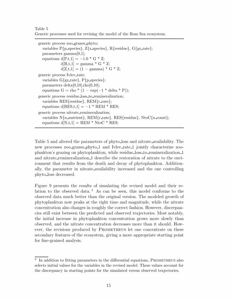
Table 5Generic processes used for revising the model of the Ross Sea ecosystem.

generic process zoo grazes phyto;variables P{p species}, Z{z species}, R{residue}, G{gz rate};parameters gamma[0,1];equations d[P,t,1] = −1.0 * G * Z;

d[R,t,1] = gamma * G * Z;d[Z,t,1] = (1 − gamma) * G * Z;

generic process Ivlev rate;variables G{gz rate}, P{p species};parameters delta[0,10],rho[0,10];equations G = rho * (1 − exp(−1 * delta * P));

generic process residue loss to remineralization;variables RES{residue}, REM{r rate};equations d[RES,t,1] = −1 * REM * RES;

generic process nitrate remineralization;variables N{n nutrient}, REM{r rate}, RES{residue}, NtoC{n const};equations d[N,t,1] = REM * NtoC * RES;

Table 5 and altered the parameters of phyto loss and nitrate availability. Thenew processes zoo grazes phyto 1 and Ivlev rate 1 jointly characterize zoo-plankton’s grazing on phytoplankton, while residue loss to remineralization 1and nitrate remineralization 1 describe the restoration of nitrate to the envi-ronment that results from the death and decay of phytoplankton. Addition-ally, the parameter in nitrate availability increased and the one controllingphyto loss decreased.

Figure 9 presents the results of simulating the revised model and their re-lation to the observed data. 4 As can be seen, this model conforms to theobserved data much better than the original version. The modeled growth ofphytoplankton now peaks at the right time and magnitude, while the nitrateconcentration also changes in roughly the correct fashion. However, discrepan-cies still exist between the predicted and observed trajectories. Most notably,the initial increase in phytoplankton concentration grows more slowly thanobserved, and the nitrate concentration decreases more than it should. How-ever, the revisions produced by Prometheus let one concentrate on thesesecondary features of the ecosystem, giving a more appropriate starting pointfor fine-grained analysis.

4 In addition to fitting parameters in the differential equations, Prometheus alsoselects initial values for the variables in the revised model. These values account forthe discrepancy in starting points for the simulated versus observed trajectories.

15

Table 6Processes that were either altered or added by Prometheus to the original RossSea model.

process zoo grazes phyto 1;equations d[phyto,t,1] = −1 * G * zoo;

d[residue,t,1] = 0.914228 * G * zoo;d[zoo,t,1] = (1 − 0.914228) * G * zoo;

process Ivlev rate 1;equations G = 2.232819 * (1 − exp(−1 * 0.004399 * phyto));

process residue loss to remineralization 1;equations d[residue,t,1] = −1 * remin rate * residue;

process nitrate remineralization 1;equations d[nitrate,t,1] = remin rate * nitrate to carbon ratio * residue;

process phyto loss;equations d[phyto,t,1] = −0.017099 * phyto;

d[residue,t,1] = 0.017099 * phyto;

process nitrate availability;equations nitrate rate = nitrate / (nitrate + 9.804389);

6 Modeling Photosynthesis Regulation with Prometheus

In addition to the two ecosystems already described, we used Prometheus

to investigate the regulation of photosynthesis. Biologists have devoted a largeamount of time to this system, and they continue to investigate the underlyingmechanisms. Recently, Labiosa et al. (2003) examined photosynthetic behav-ior within the cyanobacterium Synechocystis sp. PCC 6803. Their experimentssimulated natural lighting conditions and sampled the bacteria at nine pointswithin a 24-hour period. They processed these samples using cDNA microar-ray technology, and measured mRNA concentrations for numerous genes. Weused Prometheus to build a plausible model of photosynthesis regulation,to analyze the microarray data, and to revise this model.

Fig. 9. Observed concentrations of phytoplankton and nitrate, along with valuespredicted by the revised model of the Ross Sea ecosystem.

16

Table 7 displays the initial model of photosynthesis regulation, which relatessix variables. The first represents the amount of light available to the observedplants throughout the day. As in the Ross Sea model, the amount of light issimulated using a trigonometric function, which ensures that the light intensitypeaks at noon. The next three variables represent concentrations of mRNA,photosynthetic protein, and reactive oxygen species (ROS), respectively. ThemRNA variable encodes an aggregate over 17 genes that were implicated inregulation of the photosynthetic system, whereas both photosynthetic proteinand ROS are biologically plausible theoretical terms. The former denotes theaverage concentration of all proteins involved in photosynthesis, whereas thelatter represents the amount of a damaging byproduct the process produces.The final two variables signify the amount of energy in the system (redox) andthe rate of mRNA transcription.

The eight processes in the initial model are similar in form to those we havepreviously discussed. Photosynthesis produces both redox and ROS. Transla-tion increases the amount of protein, while transcription increases the mRNAconcentration while consuming redox. The negative effect of ROS on proteinis captured in protein degradation ros, and the normal degradation of mRNAis represented by mRNA degradation.

Unlike the other models, some of the processes in Table 7 have conditions,which are stated as arithmetic relations placed before the equations and sep-arated by commas. During simulation, a process is active only when all of itsconditions are met. As an example, mRNA degradation cannot occur unlessmRNA is present, so the model explicitly requires a positive mRNA concen-tration for the degradation process to proceed.

Figure 10 shows how Prometheus displays the process model for photosyn-thesis regulation. This graphical representation reveals three primary path-ways that are tied together by three processes. The lighting pathway providesinput to photosynthesis and affects the amount of mRNA by influencing thetranscription rate. The pathway containing ROS and photosynthetic proteindescribes how protein concentrations decrease within the cell as affected bythe amount of mRNA through photo translation. The last pathway describesthe change in mRNA due to the amount of cellular energy. All three inter-act through the central photosynthesis process that uses light and producesboth ROS, which lowers the protein concentration, and redox, which increasesmRNA transcription.

Figure 11 presents the simulated results from the model compared with theobserved mRNA values. As in the data, the predicted trajectory has two peaks,with a striking drop in mRNA concentration at noon. However, both themagnitude and timing of the events are incorrect. The first peak produced bythe model occurs too early in the day, and the last peak both occurs too late

17

Table 7The initial model of photosynthesis regulation.

model Photosynthesis Regulation;

variables light{light}, mRNA{mRNA}, transcription rate{rate},ROS{ros}, redox{redox}, photo protein{photo protein};

observable mRNA;

process photosynthesis;equations d[redox,t,1] = 1.50 * light * photo protein;

d[ROS,t,1] = 1.00 * light * photo protein;

process photo translation;equations d[photo protein,t,1] = 0.20 * mRNA;

process protein degradation ros;conditions photo protein > 0, ROS > 0;equations d[photo protein,t,1] = −0.05 * ROS;

d[ROS,t,1] = −0.05 * ROS;

process mRNA transcription;equations d[mRNA,t,1] = transcription rate;

process regulate light;equations transcription rate = 0.80 * light;

process regulate redox;conditions redox > 0;equations transcription rate = −2.00 * redox;

d[redox,t,1] = −1.00 * redox;

process mRNA degradation;conditions mRNA > 0;equations d[mRNA,t,1] = −0.02 * mRNA;

process lighting;equations light = 1 − cos((2 * 3.1415926 / 24) * t);

and overshoots the observed maximum concentration. Even more distressingis that the concentration of mRNA dips below zero for several hours. Eachof these discrepancies in the simulated trajectory indicates that we shouldattempt to revise the model.

In earlier work (Langley et al., 2006), we reported the model in Table 8, whichprovides an improved fit to the data. Structurally, this model differs from thatin Table 7 due to the absence of regulate light. Originally, the amount of lightaffected mRNA translation directly, but the revised version posits that lighthas only an indirect effect due to its influence on redox. In addition to thisstructural change, Prometheus altered the parameters of all the processes.The resulting model leads to the behavior shown on the right in Figure 11,which fits the observations almost perfectly. 5

5 We have not reported the observed data because our biologist collaborators havenot yet published them. Also, given the noise inherent in microarrays, such a good

18

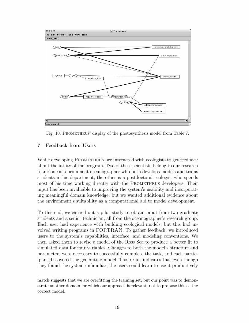
Fig. 10. Prometheus’ display of the photosynthesis model from Table 7.

7 Feedback from Users

While developing Prometheus, we interacted with ecologists to get feedbackabout the utility of the program. Two of these scientists belong to our researchteam: one is a prominent oceanographer who both develops models and trainsstudents in his department; the other is a postdoctoral ecologist who spendsmost of his time working directly with the Prometheus developers. Theirinput has been invaluable to improving the system’s usability and incorporat-ing meaningful domain knowledge, but we wanted additional evidence aboutthe environment’s suitability as a computational aid to model development.

To this end, we carried out a pilot study to obtain input from two graduatestudents and a senior technician, all from the oceanographer’s research group.Each user had experience with building ecological models, but this had in-volved writing programs in FORTRAN. To gather feedback, we introducedusers to the system’s capabilities, interface, and modeling conventions. Wethen asked them to revise a model of the Ross Sea to produce a better fit tosimulated data for four variables. Changes to both the model’s structure andparameters were necessary to successfully complete the task, and each partic-ipant discovered the generating model. This result indicates that even thoughthey found the system unfamiliar, the users could learn to use it productively

match suggests that we are overfitting the training set, but our point was to demon-strate another domain for which our approach is relevant, not to propose this as thecorrect model.

19

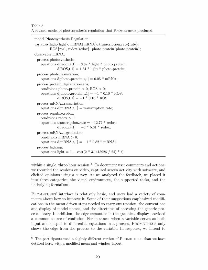
Table 8A revised model of photosynthesis regulation that Prometheus produced.

model Photosynthesis Regulation;

variables light{light}, mRNA{mRNA}, transcription rate{rate},ROS{ros}, redox{redox}, photo protein{photo protein};

observable mRNA;

process photosynthesis;equations d[redox,t,1] = 3.62 * light * photo protein;

d[ROS,t,1] = 1.34 * light * photo protein;

process photo translation;equations d[photo protein,t,1] = 0.05 * mRNA;

process protein degradation ros;conditions photo protein > 0, ROS > 0;equations d[photo protein,t,1] = −1 * 0.10 * ROS;

d[ROS,t,1] = −1 * 0.10 * ROS;

process mRNA transcription;equations d[mRNA,t,1] = transcription rate;

process regulate redox;conditions redox > 0;equations transcription rate = −12.72 * redox;

d[redox,t,1] = −1 * 5.31 * redox;

process mRNA degradation;conditions mRNA > 0;equations d[mRNA,t,1] = −1 * 0.82 * mRNA;

process lighting;equations light = 1 − cos((2 * 3.1415926 / 24) * t);

within a single, three-hour session. 6 To document user comments and actions,we recorded the sessions on video, captured screen activity with software, andelicited opinions using a survey. As we analyzed the feedback, we placed itinto three categories: the visual environment, the supported tasks, and theunderlying formalism.

Prometheus’ interface is relatively basic, and users had a variety of com-ments about how to improve it. Some of their suggestions emphasized modifi-cations in the menu-driven steps needed to carry out revision, the conventionsand display of model names, and the directness of accessing the generic pro-cess library. In addition, the edge semantics in the graphical display provideda common source of confusion. For instance, when a variable serves as bothinput and output to differential equations in a process, Prometheus onlyshows the edge from the process to the variable. In response, we intend to

6 The participants used a slightly different version of Prometheus than we havedetailed here, with a modified menu and window layout.

20

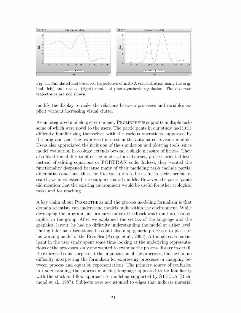
Fig. 11. Simulated and observed trajectories of mRNA concentration using the orig-inal (left) and revised (right) model of photosynthesis regulation. The observedtrajectories are not shown.

modify the display to make the relations between processes and variables ex-plicit without increasing visual clutter.

As an integrated modeling environment, Prometheus supports multiple tasks,some of which were novel to the users. The participants in our study had littledifficulty familiarizing themselves with the various operations supported bythe program, and they expressed interest in the automated revision module.Users also appreciated the inclusion of the simulation and plotting tools, sincemodel evaluation in ecology extends beyond a single measure of fitness. Theyalso liked the ability to alter the model at an abstract, process-oriented levelinstead of editing equations or FORTRAN code. Indeed, they wanted thefunctionality deepened because many of their modeling tasks include partialdifferential equations; thus, for Prometheus to be useful in their current re-search, we must extend it to support spatial models. However, the participantsdid mention that the existing environment would be useful for other ecologicaltasks and for teaching.

A key claim about Prometheus and the process modeling formalism is thatdomain scientists can understand models built within the environment. Whiledeveloping the program, our primary source of feedback was from the oceanog-rapher in the group. After we explained the syntax of the language and thegraphical layout, he had no difficulty understanding the model at either level.During informal discussions, he could also map generic processes to pieces ofhis working model of the Ross Sea (Arrigo et al., 2003). Although each partic-ipant in the user study spent some time looking at the underlying representa-tions of the processes, only one wanted to examine the process library in detail.He expressed some surprise at the organization of the processes, but he had nodifficulty interpreting the formalism for expressing processes or mapping be-tween process and equation representations. The primary source of confusionin understanding the process modeling language appeared to be familiaritywith the stock-and-flow approach to modeling supported by STELLA (Rich-mond et al., 1987). Subjects were accustomed to edges that indicate material

21

flow between variables as opposed to causal influences. As a result, we planto incorporate a second graphical view that better matches stock-and-flow di-agrams, thus providing a familiar representation to help ecologists interprettheir models.

The user study provided generally encouraging results, but it also suggestedextensions that should make Prometheus more useful to domain scientists.In summary, the users appreciated the ability to search through a space ofmodel structures and liked the integration of multiple model-related tools.However, their comments about spatial modeling and the visual representationof the model indicated obvious areas for improvement.

8 Related Research on Modeling and Discovery

In the preceding text, we illustrated both the structure of quantitative pro-cess models and the capabilities of Prometheus. We introduced a formalismthat lets a scientist represent mechanisms as networks of variables and familiarprocesses, along with an environment that displays the causal structure of themodel and simulates its behavior. If the simulated trajectories fail to match ob-served data, the user can ask Prometheus to propose revisions that improveits fit in ways consistent with domain knowledge. Generic processes providethe link in these revision efforts, giving the ability to produce explanatorymodels, as opposed to simply descriptive ones. This combination of featuresdistinguishes the system from other quantitative modeling environments.

As we indicated in the introduction, Prometheus’ approach to scientificmodeling is not entirely new, but rather borrows ideas from two previouslydisconnected literatures. However, it does more than simply combine two ex-isting technologies; it moves beyond them to demonstrate new functionalityand address new issues in interface design. Here we discuss in more detail therelations between our approach and earlier work.

On the one hand, the Prometheus environment has many similarities tomodeling frameworks like STELLA (Richmond et al., 1987) and MATLAB(The Mathworks, Inc., 1997). They share the notion of a formal syntax forspecifying both instantaneous and dynamic quantitative models in terms ofmathematical equations, although their detailed notations differ. In addition,they let the user create and edit models in this syntax, as well as invoke an as-sociated simulator that can run those models to generate predictions. Finally,they all provide a graphical interface that lets the user display and inspect thelogical structure of his mathematical models. Our approach also shares manyfeatures with Keller’s (1995) SIGMA, which is another graphical environmentthat takes an interactive approach to model building, visualization, and anal-

22

ysis, as well as providing extensive checks to ensure model consistency and tohandle unit conversions.

However, Prometheus moves beyond these earlier modeling environmentsby requiring the user to organize equations into processes. This idea plays acentral role in many scientific disciplines and appears in qualitative modelingtools such as Homer (Bredeweg and Forbus, 2003), but previous quantita-tive simulation languages have not supported it. Equally important, the newenvironment supports computational revision of models in response to data,constrained by domain knowledge in the form of generic processes and byinput from the user. MATLAB includes some facilities for attempting to esti-mate a model’s parameters for a given data set, but it cannot alter the basicstructure of a model.

At the same time, Prometheus incorporates many ideas from earlier workon computational scientific discovery. In particular, it adopts the metaphor ofheuristic search through a space of candidate structures guided by their abilityto fit data. Our approach differs from other quantitative discovery work (e.g.,Langley et al., 1987; Washio and Motoda, 1998) by focusing on process models,rather than on independent sets of equations, and by emphasizing revision ofmodels rather than their generation, although it borrows ideas on this frontfrom other efforts. Early research in this area emphasized qualitative models(e.g., Ourston and Mooney, 1990; Towell, 1991), although some more recentwork addresses quantitative models with numeric equations (e.g., Chown andDietterich, 2000; Saito et al., 2001; Todorovski and Dzeroski, 2001).

The environment also differs from most earlier discovery research by its re-liance on explicit domain knowledge to constrain search. Easley and Bradley(1999) take a similar approach in that their system uses generalized physical

networks, which take the form of general equations, as background knowl-edge to discover differential equation models of nonlinear dynamic systems.Similarly, Todorovski and Dzeroski’s (1997) Lagramge encodes backgroundknowledge in terms of context-free grammars that specify the space of equa-tions to consider during its search for models. Prometheus draws on a similaridea, but employs domain knowledge in terms of generic processes rather thanthese other formalisms, as has Todorovski’s (2003) recent work.

But the main difference from earlier discovery research concerns the interactivenature of our environment. Previous work on computational scientific discov-ery has focused almost exclusively on automated methods, whereas Prome-

theus aims explicitly to support scientists rather than to replace them. Thisphilosophy is consistent with a general trend in artificial intelligence researchtoward advisory systems, but it means we have had to address issues abouthuman–computer interaction (e.g., how best to let users constrain the searchfor revised models) that some algorithm-oriented researchers will find unin-

23

teresting. Nevertheless, such issues must receive serious attention if we hopeto develop computational discovery tools that practicing scientists will use ona regular basis.

We should note that our environment is not quite the first designed to acceptuser input. 7 For example, Valdes-Perez (1995) developed Mechem, whichfinds chemical reaction pathways that explain how a set of reactants produce aset of observed products. In addition to background knowledge about catalyticchemistry, the system accepts input from the user about constraints, expressedin terms familiar to chemists, that the inferred pathways must satisfy. Theuser can only influence Mechem’s behavior by setting switches before a run,not in an on-line manner, as we envision for the Prometheus environment.Nevertheless, the system has produced a number of novel reaction pathwaysthat have appeared in the chemistry literature.

Another example is Mitchell et al.’s (1997) Daviccand, which was designedto discover quantitative relations in metallurgy. This system encourages theuser to actively direct the search process and provides explicit control pointswhere he can influence choices. In particular, the user formulates a problemby specifying the dependent variable the laws should predict, the region ofthe space to consider, and the independent variables to use when lookingfor numeric laws. The user can also manipulate the data by selecting whichpoints to treat as outliers. Daviccand presents its results in terms of graphicaldisplays and functional forms that are familiar to metallurgists, and the systemhas produced knowledge published in their literature.

The research that appears closest to our own comes from Mahidadia andCompton (2001), who report an integrated environment for the developmentand revision of qualitative causal models. Their system provides a graphicalinterface for model construction and visualization that maps well onto modelsin their target domain, neuroendocrinology. The JustAid system starts withan initial model provided by the user and, using experimental data about theeffects of independent variables on dependent measures, recommends changesto this model in terms of link additions and deletions, which the user mustapprove before they are implemented. The main functional difference betweenJustAid and Prometheus are that the former supports qualitative models,stated as signed links between continuous variables, whereas the latter dealswith quantitative process models. Their underlying algorithms also differ, butthese are far less visible to users than the model formalism and interface.

7 A number of commercial environments for knowledge discovery also support userinteraction, but, besides focusing on business applications, these emphasize decisionsabout how to preprocess the data and which algorithm to run on them.

24

9 Directions for Future Research

Although Prometheus breaks new ground in computer-assisted modelingand discovery, we must still extend it along a number of dimensions beforeit becomes a robust tool for practicing scientists. One limitation is that thecurrent framework only supports models at one level of description, whichmeans that it is most appropriate for situations that involve relatively fewvariables and processes. A natural response is to expand the modeling languageto incorporate the notion of subsystems that characterize components of theoverall model. For example, an ecosystem model might include one subsystemfor water-related processes and another for sunlight-related processes. This“decompositional” approach would let users hide information and help themmanage more complex models by letting them focus both their own attentionand that of Prometheus’ revision module on one subsystem at a time.

Other extensions would augment the background knowledge available to theenvironment, which is currently limited to a taxonomy of variables that islinked to a set of generic processes. Future versions of Prometheus shouldincorporate dimensional information about classes of variables, which wouldgive the system enough knowledge to check models more carefully for cor-rectness and convert units across processes that use different measures. Thesystem should also support a taxonomy of processes to provide the user withmore flexibility to direct model revision. For instance, such a taxonomy mightinclude generic processes like ‘growth’ at higher levels that specify only quali-tative proportions between variables, whereas processes at lower levels wouldencode specialized types like ‘exponential growth’ that give the forms of nu-meric equations. Such a hierarchy would let users identify either the abstractprocesses or the more concrete ones as candidates for revision. More generally,the environment should also support the creation and revision of qualitativemodels, which are especially appropriate for domains with limited data.

The current implementation of Prometheus relies on a single revision al-gorithm, but this is certainly not a logical necessity. In future versions, weplan to incorporate other discovery algorithms that would broaden the meth-ods available for model revision, which in turn should make this facility morerobust and effective. Additionally, we recognize that scientists will need tomanually edit the models that the program produces (e.g., to account for mi-nor discrepancies as discussed at the end of Section 5). In response, we shouldinclude tools that ease parameter tuning and sensitivity analysis, which willhelp the scientist better understand the interrelationships within the model.We should also extend the Prometheus environment to move beyond modelrevision to support the induction of process models from generic componentsand data, as we have described elsewhere (Langley et al., 2003).

25

Finally we plan to modify Prometheus’ interface based on the results of ouruser study. Currently, users instantiate processes by selecting a generic pro-cess from a list and specifying the variable bindings and parameter values ina dialog window. Ideally, this activity should take on a more visual character.Research on educational modeling tools such as IQON (Miller et al., 1993)and VModel (Bredeweg and Forbus, 2003) suggests possible improvementsin this direction. Prometheus also needs tools that help the user understandthe deep nature of the relationships among variables. Although the programcan produce simulated trajectories, the user must engage in tedious parame-ter tuning to explore the behavior of a particular model structure. To enablemore meaningful exploration of the structure, the environment could create aqualitative version of the model and use a tool like VisiGarp (Salles, 2003) tolet the user see the effects of large-scale changes without worrying about para-metric details. Such additions will bring the environment closer to a flexibleand robust tool that domain scientists would readily adopt and use.

10 Concluding Remarks

In this paper, we presented a new framework for modeling and discovering sci-entific knowledge, along with Prometheus, an interactive environment thatimplements this approach. The environment includes a language for specifyingquantitative models in which the notion of process plays a central role. Thisformalism takes advantage of traditional scientific notations like algebraic anddifferential equations, but provides additional structure to aid in presentingand revising models. We illustrated the process modeling language with ex-amples from three domains, which also clarified the interactive features ofPrometheus. These include options for visualizing the causal structure ofprocess models, for simulating these models to generate predictions, for visu-alizing the resulting behavior of models, and for semi-automatically revisingmodels in response to observations. The latter facility lets the user specify theportions of a model to revise and indicate additional processes, taken from alibrary of generic background knowledge, that the system should consider.

We evaluated this approach to model revision on two domains that concernedinteractions within an ecosystem and one that involved gene regulation. Usinga simple predator–prey ecosystem, we demonstrated that Prometheus canproduce revised models that yield improvements to both the qualitative shapeand quantitative error score with respect to the original model. Application tothe Ross Sea ecosystem indicated that the environment’s revision capabilitiesscale up to represent more complicated interactions, whereas revision of aphotosynthesis-regulation model supported the generality of the approach. Inaddition, ecologists who worked with Prometheus were interested in therevision module and found its output understandable.

26

Although our development of Prometheus is still in its early stages, we be-lieve the environment makes important contributions to simulation languages,to human–computer interaction, and to computational scientific discovery. Ourinitial results with the system have been encouraging and, despite the roomthat remains for extensions and improvements, we feel that they demonstratethe promise of such an interactive framework for computer-assisted construc-tion and use of scientific models.

Acknowledgements

The research reported in this paper was supported in part by NTT Commu-nication Science Laboratories, Nippon Telegraph and Telephone Corporation,in part by Grant NCC 2-1220 from NASA Ames Research Center, and in partby Grant No. IIS-0326059 from the National Science Foundation. We thankNima Asgharbeygi and Xumei Marker for their early work on the environ-ment’s component algorithms, along with Saso Dzeroski, Ljupco Todorovski,Kazumi Saito, and Daniel Shapiro for discussions that led to many of the ideasin this paper. We also thank Kevin Arrigo and Stuart Borrett for assistancewith the ecological aspects of the research.

References

Arrigo, K.R., Worthen, D.L., Robinson, D.H., 2003. A coupled ocean–ecosystem model of the Ross Sea: 2. Iron regulation of phytoplankton taxo-nomic variability and primary production. Journal of Geophysical Research108 (C7), 3231.

Asgharbeygi, N., Langley, P., Bay, S., 2006. Inductive revision of quantitativeprocess models. Ecological Modeling 194, 70–79.

Bredeweg, B., Forbus, K.D., 2003. Qualitative modeling in education. AI Mag-azine 24, 35–46.

Chown, E., Dietterich, T.G., 2000. A divide and conquer approach to learn-ing from prior knowledge, in: Proceedings of the Seventeenth InternationalConference on Machine Learning. Morgan Kaufmann, San Francisco, CA,143–150.

Easley, M., Bradley, E., 1999. Generalized physical networks for automatedmodel building, in: Proceedings of the Sixteenth International Joint Con-ference on Artificial Intelligence. Morgan Kaufmann, 1047–1053.

Fayyad, U., Piatetsky-Shapiro, G., Smyth, P., 1996. From data mining toknowledge discovery in databases. AI Magazine 17, 37–54.

Forbus, K.D., 1984. Qualitative process theory. Artificial Intelligence 24, 85–168.

27

Forbus, K.D., Falkenhainer, B., 1990. Self-explanatory simulations: An inte-gration of qualitative and quantitative knowledge. in: Proceedings of theEigth National Conference on Artificial Intelligence. AAAI Press, 380–387.

Jost, C., Ellner, S., 2000. Testing for predator dependence in predator–preydynamics: A nonparametric approach. Proceedings of the Royal Society ofLondon: Biological Sciences 267, 1611–1620.

Keller, R.M., 1995. An intelligent visual programming environment for scien-tific modeling. Science Information Systems Newsletter 35.

Labiosa, R., Arrigo, K., Grossman, A., Reddy, T.E., Shrager, J., 2003. Diurnalvariations in pathways of photosynthetic carbon fixation in a freshwatercyanobacterium, presented at European Geophysical Society Meeting. Nice,France.

Langley, P., 2000. The computational support of scientific discovery. Interna-tional Journal of Human–Computer Studies 53, 393–410.

Langley, P., Shiran, O., Shrager, J., Todorovski, L., Pohorille, A., 2006. Con-structing explanatory process models from biological data and knowledge.Artificial Intelligence in Medicine 37, 191–201.

Langley, P., George, D., Bay, S., Saito, K., 2003. Robust induction of processmodels from time-series data, in: Proceedings of the Twentieth InternationalConference on Machine Learning. Washington, DC, 432–439.

Langley, P., Simon, H.A., Bradshaw, G.L., Zytkow, J.M., 1987. Scientific dis-covery: Computational explorations of the creative processes. MIT Press,Cambridge, MA.

Levenberg, K., 1944. A method for the solution of certain problems in leastsquares. Quarterly of Applied Mathematics 2, 164–168.

Mahidadia, A., Compton, P., 2001. Assisting model discovery in neuroen-docrinology, in: Proceedings of the Fourth International Conference on Dis-covery Science. Springer, 214–227.

Marquardt, D., 1963. An algorithm for least-squares estimation of nonlinearparameters. SIAM Journal of Applied Mathematics 11, 431–441.

Miller, R., Ogborn, J., Briggs, J., Brough, D., Bliss, J., Boohan, R., Brosnan,T., Mellar, H., Sakonidis, B., 1993. Educational tools for computationalmodelling. Computers in Education 21, 205–261.

Mitchell, F., Sleeman, D., Duffy, J.A., Ingram, M.D., Young, R.W., 1997.Optical basicity of metallurgical slags: A new computer-based system fordata visualisation and analysis. Ironmaking and Steelmaking 24, 306–320.

Ourston, D., Mooney, R., 1990. Changing the rules: A comprehensive approachto theory refinement, in: Proceedings of the Eighth National Conference onArtificial Intelligence. AAAI Press, Boston, MA, 815–820.

Richmond, B., Peterson, S., Vescuso, P., 1987. An academic user’s guide toSTELLA. High Performance Systems, Lyme, NH.

Saito, K., Langley, P., Grenager, T., Potter, C., Torregrosa, A., Klooster, S.A.,2001. Computational revision of quantitative scientific models, in: Proceed-ings of the Fourth International Conference on Discovery Science. Springer,336–349.

28

Shneiderman, B., 2000. Creating creativity: User interfaces for supporting in-novation. ACM Transactions of Computer-Human Interaction 7, 114–138.

Salles, P., Bredeweg, B., 2003. Qualitative reasoning about population andcommunity ecology. AI Magazine 24, 77–90.

The MathWorks, Inc., 1997. Simulink user’s guide: Dynamic system simula-tion for MATLAB. Natick, MA.

Todorovski, L., 2003. Using domain knowledge for automated modeling ofdynamic systems with equation discovery. Doctoral Dissertation, Faculty ofComputer and Information Science, University of Ljubljana, Slovenia.

Todorovski, L., Dzeroski, S., 1997. Declarative bias in equation discovery, in:Proceedings of the Fourteenth International Conference on Machine Learn-ing. Morgan Kaufmann, Nashville, TN, 376–384.

Todorovski, L., Dzeroski, S., 2001. Theory revision in equation discovery, in:Proceedings of the Fourth International Conference on Discovery Science.Springer, Washington, DC, 389–400.

Towell, G., 1991. Symbolic knowledge and neural networks: Insertion, refine-ment, and extraction. Doctoral dissertation Computer Sciences Department,University of Wisconsin, Madison, WI.

Valdes-Perez, R.E., 1995. Machine discovery in chemistry: New results, Arti-ficial Intelligence 74, 191–201.

Washio, T., Motoda, H., 1998. Discovering admissible simultaneous equationsof large scale systems, in: Proceedings of the Fifteenth National Conferenceon Artificial Intelligence. AAAI Press, Madison, WI, 189–196.

29