an intelligent active range sensor for … local processing provides greater autonomy, ... the...

Pergamon

Mechatronics Vol, 6, No. 7, pp. 733-759, 1996 Copyright © 1996 Elsevier Science Ltd. All rights reserved.

Printed in Great Britain. 0957-4158/96 $15.00+0.00

PII:S0957-4158 (96) 00022-0

AN INTELLIGENT ACTIVE RANGE SENSOR FOR MOBILE ROBOT GUIDANCE

N. E. PEARS* and P. J. PROBERT* *Department of Engineering, University of Cambridge, Trumpington Street, Cambridge

CB2 1PZ, U.K. and *Department of Engineering, University of Oxford, Parks Road, Oxford OX1 3PJ, U.K.

(Received 13 July 1995; accepted 20 December 1995)

Abstract--The mechatronic design of an eye-safe laser rangefinder, based on the lateral-effect photodiode (LEP) and synchronised scanning, is described. The sensor acquires two-dimensional range data, which has been found sufficient to guide the local manoeuvres of a mobile robot in most environments. An analysis of LEP operation shows that image position measurement repeatability, normalised with respect to the detector half length, is equal to the signal current to noise current ratio. This result suggests a method for estimating the noise density of the measurement process and, along with a geometric model of the ranging process, allows accurate estimation of the variance of individual range measurements, making the sensor particularly amenable to statistically based range feature detection, tracking, and data fusion algorithms. The sensor is active, in the sense that it can change the orientation of its field of view, in order to track useful and stable range features. Range data acquisition, range feature extraction, and control of the active head behaviour are all implemented on a local network of six transputers. This parallel structure is described and it is shown how the sensor constitutes an intelligent agent in a balanced sensor suite for the guidance of close range mobile robot manoeuvres. Copyright (~) 1996 Elsevier Science Ltd.

1. INTRODUCTION

Robotic systems, which handle large amounts of sensor data from a number of often disparate sources, require a processing structure which is distributed in order to operate in real-time. A logical and modular way to distribute processing is to dedicate one or more processing units to each data stream entering the system so that only the salient features and associated uncertainties of that data need to be presented to the rest of the robotic system. If the sensor creating the data stream is active, in the sense that it can change its position and orientation in order to extract the maximum amount of information relevant to the current task and the information extracted locally can guide such position changes, then the sensor and associated processing units form ~in intelligent sensor. Such sensors operate as modular units within a distributed robotic system,

In the Oxford Autonomous Guided Vehicle (AGV) project, a number of such

733

734 N.E. PEARS and P. J. PROBERT

sensors have been built into a common distributed processing platform called the locally intelligent control agent (LICA) architecture [1], which is essentially an extremely flexible on-board transputer based real-time embedded processing system. The sensors are complementary and, in addition to the senor described here, include eight steerable sonar, an active vision stereo head and a laser bar code scanner, all of which "plug in" to this architecture to form a well balanced sensor suite. A large suite of sensors on a single flexible architecture has allowed sensor planning and sensor integration to be implemented on a number of different levels for the purpose of mobile robot navigation.

The motivation for the lateral-effect photodiode (LEP) rangefinder was to build a reliable obstacle avoidance capability into an autonomous guided vehicle for factory use. The type of vehicle for which the intelligent sensor is intended is one which already has a reliable means of global position measurement in the form of a rotating bar code reader, which allows position and orientation to be triangulated. Such a system cannot avoid anything that is not accurately incorporated into a map based around the bar code positions. The provision of an additional sensor and its associated local processing provides greater autonomy, allowing many everyday circumstances in the factory to be tackled without any form of human intervention. The LEP rangefinder acquires two-dimensional range data, which is abstracted into a piecewise linear model of the environment. This has been found sufficient for local manoeuvres in most environments.

In the following section, a number of different ranging methods are compared, illustrating why optical triangulation is particularly suitable for our ranging application. The sensor design, described in section 3, combines a number of technologies, which include low noise amplification, lock-in detection and synchronous scanning, in order to extend the application domain of LEPs into mobile robotics. Previously, such devices have been used over smaller depths of field and/or have used non eye-safe lasers. Section 4 details both the calibration procedure and the measured performance specification. The following section gives a theoretical analysis of sensor performance. Firstly, this is necessary to predict the performance of the sensor, which allows both feasibility testing at the design stage, and a means of vindicating the design by comparing it with the measured sensor performance. Secondly, the analysis provides a means of estimating range variance in order to apply statistically based range feature extraction to the raw range data. A final section before the conclusions details how the sensor is integrated into the LICA architecture, and outlines how line segments are extracted recursively and used to guide both the sensor head orientation and the vehicle.

2. A REVIEW OF RANGE MEASUREMENT TECHNIQUES

Passive vision provides the most comprehensive source of sensory information from a single sensing device; however, the projection of a three-dimensional scene into a two-dimensional image engenders ambiguity, making range recovery difficult. Several different cues have been exploited to recover range, such as stereo disparity [2], and visual motion [3]. However, the use of passive vision is often precluded, since the large bandwidth of raw data requires fast, potentially expensive processing hardware

Intelligent active range sensor for mobile robot guidance 735

to extract the required range information. Sensors designed specifically for range measurement can often provide task-specific range' information at a sufficiently high rate for the real-time performance requirements more cheaply. Here, we will compare optical radar, sonar, and optical triangulation. Comprehensive reviews of ranging techniques can be found in [4, 5].

In optical radar, the phase relationship between an amplitude modulated light beam (laser, or collimated L E D ) a n d its reflection is used to calculate range [6]. In sonar, the speed of sound is sufficiently low for the round trip of pulses to be timed [7]. Optical triangulation is a geometric means of ranging and involves projecting a light source onto the scene and observing the image position of that projection with a lens/detector combination offset from the axis of projection. Scene coverage can be achieved either by scanning a spot or line stripe [8], or by projecting a pattern of dots or lines [9] onto the area of interest.

Sonar has a number of disadvantages when compared to optical methods. Firstly, the low speed of sound means that range measurements can only be made at a low rate (10-100 Hz, depending on range). Secondly, its large wavelength means it suffers from specularities. This means that the spatial density of measurements is low, since only certain parts of the scene can be detected, such as cylinders, comers, and planar surfaces which are oriented within the effective beamwidth of the ultrasonic pulse. Thirdly, specularity in combination with a large beamwidth engenders ambiguity in the angle of the range measurement. For these reasons, we believe that sonar sensing is unsuitable for guiding close range vehicle manoeuvres.

Of the optical methods of active ranging mentioned, optical radar is more practical than optical triangulation in outdoor environments where, at large ranges, triangulation becomes inaccurate. In addition, the missing parts problem, which is a characteristic of any stereo/triangulation system, is eliminated, since the transmitted and received beams are co-axial. However, over short ranges, such systems are generally of lower accuracy when compared with active triangulation systems. For this reason, we elected to design a triangulation system. General discussion of the tradeoffs involved when designing optical triangulation range sensors can be found in [10].

2.1. Complementary, cooperative sensing

Although sonar was considered unsuitable for guiding close range vehicle manoeuvres, this does not mean that sonar is unsuitable for autonomous vehicle localisation using mapped features [11], or for obstacle detection and sensor guiding. In fact, both sonar and the optically based LEP sensor are mounted on the Oxford AGV, and it is instructive to describe in what ways they are complementary, and how they can both be accommodated in a balanced sensor suite. Table 1 summarises this comparison in a variety of performance categories. The LEP sensor provides high (sub-millimetre) repeatability at close ranges, with a high spatial density of information at a high data rate, whereas sonar provides the ability of sensing at larger ranges, but is subject to speculatities, low spatial density of range information, and a low data rate. However, since these devices are cheap and simple, a number of transducers can be placed around the vehicle to provide a global surveillance ability. This makes sonar suitable for detecting the incidence of an obstacle, but it cannot provide sufficiently detailed information to plan an effective avoidance path. In this case, the sonar can direct the

736 N. E. PEARS and P. J. PROBERT

Table 1. LEP sensor and sonar comparison

Performance category LEP sensor Sonar

Sub-millimetre repeatability (lo) at 0.75 m Yes No Sub-centimetre repeatability (lo) at 1.5 m Yes Yes Long range (> 2.5 m) capability No Yes Global (360 ° ) surveillance No Yes Specularity immunity Yes No Data rate 2.5 kHz 10 Hz Spatial density of information High Low Angular resolution Good Poor

LEP to look in the direction of the obstacle to gain more detailed information, and so the two sensor systems act in a complementary fashion.

3. MECHATRONIC SENSOR DESIGN

In this section, analogue (LEP) and discrete (CCD) methods of image position measurement are compared. This is followed by a design method for determining the feasibility of using the LEP for analogue range measurements in mobile robot applications. Section 3.3 gives a description of the electronic design required for the low noise detection of LEP signals. Finally, the geometry of the range sensor and its optical and mechanical realisation are described.

3.1. Choice of image position detector

In active optical triangulation schemes, an image position measurement is required to make a range reading. The most common way to do this is with a CCD which is a discrete image sensing device. However, the lateral-effect photodiode (LEP) provides an alternative, analogue means of image position measurement. Here, the generated photocurrent is split linearly between two terminals according to the position of the centroid of light intensity, so that this position relative to the centre of the device (see Fig. 1) can be computed as

P - Ii + ~ \ 2 - ] - ~ p ~< + (1)

and the detector current is given by the sum of the two terminal currents

I0 = I1 + 12. (2)

The LEP has both benefits and drawbacks when compared to CCD technology. On the plus side, the LEP is cheaper and simpler to interface than a CCD, typically costing around £35 in total, and has no hard bandwidth limitations, such as frame rate or clock out rate, other than that set by the resistance and capacitance of the device (typically 2 MHz*). The LEP has extremely high resolution when the signal to noise

*In practice, this bandwidth has to be limited in the interests of signal to noise ratio.

Intelligent active range sensor for mobile robot guidance

+15v bias

P

737

I P

Fig. 1. The lateral-effect photodiode.

ratio is high, and so ranging is extremely accurate at short ranges and with targets of good reflectivity. It is shown that the image position on an LEP has a Gaussian noise characteristic, the variance of which can be found accurately from detector current. This makes the device amenable to statistically based algorithms for feature detection, feature tracking and data fusion (e.g. the Kalman filter). On the minus side, the LEP is both insensitive and noisy compared to a CCD. This means that at larger target ranges and with low reflectivity targets, low signal to noise ratios are encountered. The analogue structure of the LEP makes image position very sensitive to signal to noise ratio and so, in such circumstances, image position resolution is poor in comparison to a CCD.

If the image of the structured light falls over several pixels of a CCD, a curve can be fitted through the image profile to give sub-pixel accuracy. An LEP, however, integrates the signal over its surface and so provides a single image position reading which corresponds to the centroid of light intensity. On the one hand, the inherent structure of the device conveys an immediate result, the centre of the image position, without any further processing. On the other hand, information concerning image profile is lost through the integration, making the LEP susceptible to signal distortion. Results have shown that one such distortion is caused by the internal reflections inside a concave corner.

Since our obstacle avoidance function required short (0.4 m) to medium (2.5 m) ranging, we chose the LEP as our image position measurement device. However, it was necessary to check that a good performance could be achieved, whilst using a laser of low enough power to be eye-safe. The design method used to check the feasibility of an LEP based sensor is given in the following section.

3.2. Sensor performance prediction

Any given range measurement is subject to two sources of error: noise in the measurement process, which determines repeatability, and a calibration error. If we assume that the calibration error can be made sufficiently small by increasing the


number of calibration points, then the feasibility of the LEP based sensor head design for guiding close range mobile robot manoeuvres is based on whether sufficient repeatability is maintained over the desired depth of field. It should be noted that close range repeatability is particularly important, since this allows the safety margins during vehicle manoeuvres to be smaller. This, in turn, means that manoeuvres around obstacles can be made which would have otherwise been deemed as unpassable. At larger ranges (above 2 m), we only need to detect the fact that an obstacle exists, to initiate deceleration. Thus, as the vehicle approaches, features must be extracted much more accurately, and this behaviour is inherent in the sensor's operation.

The approach for determining repeatability is described in the five stages below. It should be emphasised that this procedure does not generate noise values that can be used in range feature extraction algorithms, since too many estimates (data sheet specifications) are used for it to be accurate. Rather, it provides an indication of feasibility at the design stage, and a means with which to assess the actual, empirically determined noise performance of the sensor.

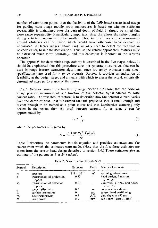
3.2.1. Detector current as a Junction o f range. Section 5.2 shows that the noise on image position measurement is a function of the detector signal current to noise current ratio. The first step, therefore, is to determine how the detector current varies over the depth of field. If it is assumed that the projected spot is small enough and distant enough to be treated as a point source and that Lambertian scattering only occurs in the scene, then the total detector current, I0, at range z can be approximated by

S 10 - , ( 3 )

9 Z-

where the parameter S is given by

S = p A cos OdT I T2R,Pj (4)

2zr

Table 2 describes the parameters in this equation and provides estimates and the source from which the estimates were made. (Note that the first three estimates are taken from the sensor head design described in section 3.4.) These estimates give an estimate of the parameter S as 24.8 n A m z.

Table 2. Sensor parameter estimates

Symbol Description Estimate Units Source of estimate

A aperture 8.8 × 10 -4 m 2 scanning mirror area T~ transmission of projection 0.73 -- head design, 3 mirrors,

optics T = 0.9 7"2 transmission of detection 0.77 -- 2 mirrors, T = 0.9 and filter,

optics T = 0.95 p scene reflectivity 0.5 -- conservative estimate 0d surface orientation 0 rad sensor head positioning R¢ LEP responsivity 0.7 A/W data sheet at 670 nm P1 laser power 0.9 mW sub 1 mW (class II limit)


3.2.2. RMS current noise density calculation. The theoretical current noise density of the detector and preamplifier combination is calculated using values of device characteristics taken from data sheets. Since these values are only an approximate reflection of the actual device characteristics, and an rms summation of noise sources has the effect of raising the threshold below which a noise source is considered insignificant, only dominant noise sources are considered. (An example of a negligible noise source is the shot noise due to any current generated by any 670 nm ambient light passing through the optical filter.)

The total current noise density associated with the detector is the rms summation of shot noise from the dark current and signal current, and the thermal noise due to its resistive layer. An estimate of signal current is taken by using the range at the centre of the depth of field (1.45 m) and applying Eqn (3) to give I 0 = 13.1 hA. For the LEP used in the sensor, dark current I d = 100 hA, Rs = 50 k•, and assuming T = 298 K

ind = ~ ( 2 e ( I d + Io) + 4 k T I = o . tpA(Hz)-I /2 . (5) Rs I

Preamplifier noise, including feedback resistor noise, is given as

• .2 en~ 4 k T tn, = tn, + + = 0.2 pA(Hz) -1/2. (6)

R s Rf ]

Calculating the rms of Eqns (5) and (6) gives the total current noise density for the detector-preamplifier combination as 0.632 pA(Hz) -1/2.

3.2.3. RMS current noise calculation. An rms noise is calculated from the rms noise density as

In = in~/(B), (7)

where B is the measurement bandwidth. This bandwidth must be chosen as a compromise between a low value of noise rejection and a high value for speed of response since the LEP signals must respond to step changes as the sensor scans over range discontinuities in the scene. In the design detailed here, a bandwidth of 1 kHz was chosen, which gives the rms current noise as 20 pA. In section 5.4, this figure is compared with an empirically determined noise current in order to vindicate the electronic design of the sensor described in section 3.3.

3.2.4. R M S image position measurement noise. Image position measurement noise can be predicted over the depth of field of the sensor by computing detector current at a number of ranges using Eqn (3). Equation (17), developed in section 5.2, can then be used to determine the rms noise in image position measurement.

3.2.5. RMS range measurement noise. The noise in image position measurement can be projected into noise in range measurement using Eqn (20), which is developed from the geometric analysis given in section 5.1. This requires estimation of the focal length, f , and triangulation baseline, d. The sensor head design gives these as 0.05 and 0.09 m respectively.


3.3. Electronic design for the low noise detection of LEP signals

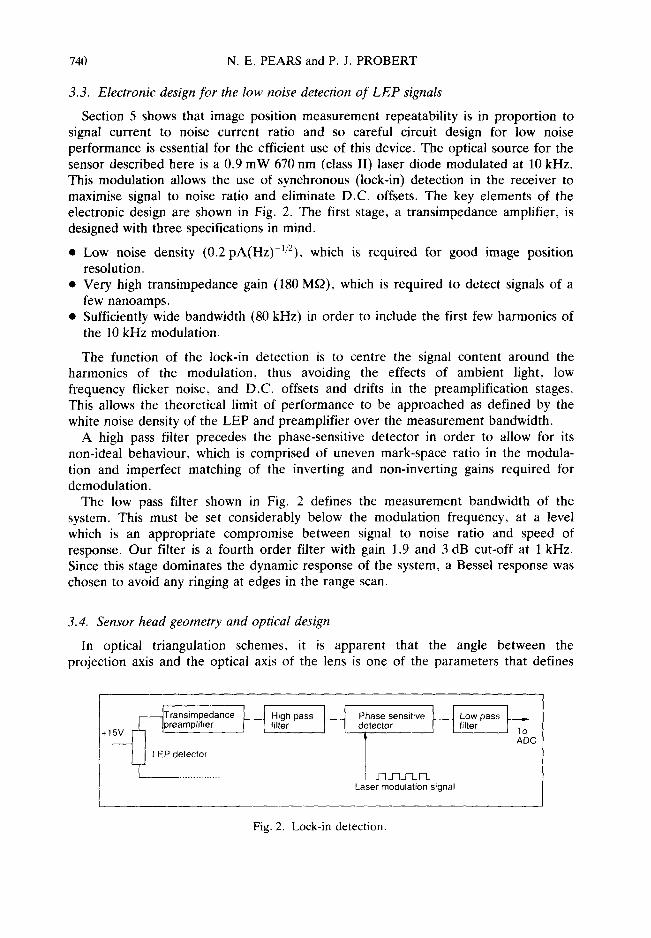
Section 5 shows that image position measurement repeatability is in proportion to signal current to noise current ratio and so careful circuit design for low noise performance is essential for the efficient use of this device. The optical source for the sensor described here is a 0.9 mW 670 nm (class II) laser diode modulated at 10 kHz. This modulation allows the use of synchronous (lock-in) detection in the receiver to maximise signal to noise ratio and eliminate D.C. offsets. The key elements of the electronic design are shown in Fig. 2. The first stage, a transimpedance amplifier, is designed with three specifications in mind.

• Low noise density (0.2pA(Hz)-l/2), which is required for good image position resolution.

• Very high transimpedance gain (180 M£2), which is required to detect signals of a few nanoamps.

• Sufficiently wide bandwidth (80 kHz) in order to include the first few harmonics of the 10 kHz modulation.

The function of the lock-in detection is to centre the signal content around the harmonics of the modulation, thus avoiding the effects of ambient light, low frequency flicker noise, and D.C. offsets and drifts in the preamplification stages. This allows the theoretical limit of performance to be approached as defined by the white noise density of the LEP and preamplifier over the measurement bandwidth.

A high pass filter precedes the phase-sensitive detector in order to allow for its non-ideal behaviour, which is comprised of uneven mark-space ratio in the modulation and imperfect matching of the inverting and non-inverting gains required for demodulation.

The low pass filter shown in Fig. 2 defines the measurement bandwidth of the system. This must be set considerably below the modulation frequency, at a level which is an appropriate compromise between signal to noise ratio and speed of response. Our filter is a fourth order filter with gain 1.9 and 3 dB cut-off at 1 kHz. Since this stage dominates the dynamic response of the system, a Bessel response was chosen to avoid any ringing at edges in the range scan.

3.4. Sensor head geometry and optical design

In optical triangulation schemes, it is apparent that the angle between the projection axis and the optical axis of the lens is one of the parameters that defines

Transimpedance + 1 ~ tpreamp tier LEP detector

I High pass ~_~ filter detectorPhase sensitive H filterL°W pass ~To

t " ADC

Laser modulation signal

Fig. 2. Lock-in detection.


the accuracy and depth of field in ranging, which is problematic if the light source is to be scanned across the scene. However, if the detection lens is scanned in synchronism with the projected light, so that their angular separation remains constant, then the performance in ranging varies very little with scan angle [12]. The implication for close range vehicle manoeuvres, such as obstacle avoidance and docking, is that a large scan angle (large field of view) can be built into the sensor design without compromising depth of field, and vigilance during vehicle movement can be maintained.

To avoid unnecessary ranging errors, it is important to ensure that the light source and detector are scanned in exact synchronism, and the best way to do this is to scan them with the same physical device: for example, with different regions on an oscillating planar mirror, or with different facets on a rotating multifaceted prismatic or pyramidal mirror, or with the two sides of a double sided oscillating planar mirror. In the latter two cases, an appropriate arrangement of stationary mirrors determines the triangulation baseline and the vergence angle.

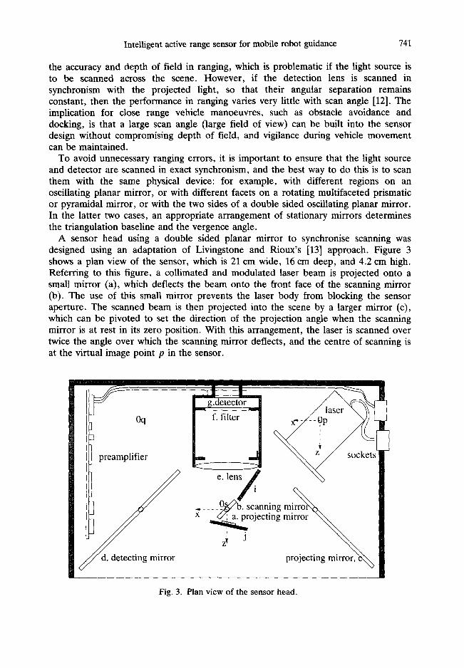
A sensor head using a double sided planar mirror to synchronise scanning was designed using an adaptation of Livingstone and Rioux's [13] approach. Figure 3 shows a plan view of the sensor, which is 21 cm wide, 16 cm deep, and 4.2 cm high. Referring to this figure, a collimated and modulated laser beam is projected onto a small mirror (a), which deflects the beam onto the front face of the scanning mirror (b). The use of this small mirror prevents the laser body from blocking the sensor aperture, The scanned beam is then projected into the scene by a larger mirror (c), which can be pivoted to set the direction of the projection angle when the scanning mirror is at rest in its zero position. With this arrangement, the laser is scanned over twice the angle over which the scanning mirror deflects, and the centre of scanning is at the virtual image point p in the sensor•

6

0q

preamplifier oc e s| e . 0 / l e n s z ~

. . . . . -O,~b. scanning m i ~ ° ~ / x ~ r ° j e c t i n g mirr°r ~ i

projecting mirror, ~ I

Fig. 3. Plan view of the sensor head.


Laser light, scattered by objects in the scene, is collected by the large adjustable detection mirror (d) and is deflected onto the rear of the scanning mirror. (This mirror is silvered on both sides.) Light leaving the scanning mirror is focussed by the lens (e) and passes through an optical filter (f), matched to the laser wavelength, before forming an image of the projected spot on the image position detector (g). To minimise noise, the detector signals are amplified inside the sensor head before being passed to the lock-in detector in the sensor interface rack.

With the geometry described above, the lens is effectively scanned around virtual image point q in the sensor on an arc with radius equal to the separation between the scanning mirror and the lens. In our design, this separation is kept as small as possible to minimise variations in triangulation baseline over the scanning range. The dimensions and positioning of the detection mirror (d) are critical and ensure that the full sensor aperture (the full surface of the scanning mirror) is accessible over all combinations of scan angle and target range.

The sensor is designed with as large an aperture as possible that is consistent with our scanning requirements because of the LEP's dependence on a good signal to noise ratio. Most of the aperture derives from the depth of the scanning mirror (4 cm) rather than its width (2.2 cm) in order to limit rotational inertia. Direct optical paths, in which laser light is focussed directly from the scene onto the LEP, have been prevented with the use of a "cats-eye" aperture stop (h) behind the lens and shielding plates (i) and (j).

3.5. Sensor head drive

The scanning optics described above is termed the sensor head. This sensor head is mounted on a servo driven platform which can rotate the field of view of the sensor head between +90 and -90 ° relative to the forward looking direction, traversing this 180 ° range in around one second, and positioning the head with an angular resolution of 0.36 °. The limits of rotation are protected by optical limit switches, whilst a third optical switch allows zeroing of the head. This head drive allows the scanning field of view to be centered at the optimal position for the current manoeuvre. For example the sensor may centre on navigable freespace or may turn so that the obstacle being avoided does not leave the scanning field of view.

4. CALIBRATION AND PERFORMANCE SPECIFICATION

In order to calibrate the sensor in the z dimension, the AGV is positioned normal to a laboratory wall, so that the range sensor is 2.5 m from the wall. It then uses its bar code scanner guidance system to move incrementally towards the wall with a predefined step size. A sample of raw scans, taken between 0.5 and 1 m, is shown in Fig. 4. (Note that, since the lens is scanned in synchronism with the laser, there is only a small variation in image position over the scanning range. Also, the fall in triangulation gain with the inverse square of target range is shown by the decreasing separation of the image position curves.) After each scare spatial filtering is applied along the scan angle dimension by application of the one-dimensional convolution operator [1,4,6,4,1]. This approach causes minimal distortion of the look-up table as a


0 . 8 ,

0 . 6

.-~ 0.4

8. 8~ t~ .E_ 0.2

- 0 . 2 . . . . . ~ . ~ , ~ . ~ ' ~

,t t i i I t i L -0"-20 -15 -10 -5 0 5 10 15 20

scan angle (degrees)

~=0.5m

~.=0.6m

~.=0.7m

.~:O.8m

~.=0.gm

,-=1 .Om

Fig. 4. Calibration curves: image position against scan angle.

model of the ranging process, since image position data is much denser in the scan angle axis than the range axis (256 data points compared to around 40), and the non-linearity is less severe. After N moves, a two-dimensional look-up table of dimension 256 angles by N range values has been built. Subsequently, range can be calculated as

z = Tz(p , 0), (8)

where T z represents an interpolation in the calibration look-up table. The second stage of calibration occurs concurrently with that of the range

dimension and is for the x dimension, which is normal to the range dimension and in the plane of the laser scan. During the advance of the AGV towards the target wall, points along the two peripheral scan lines, which correspond to scan angle 0 and scan angle 255, are measured in (x, z) coordinates in the sensor frame, which has its origin at the centre of rotation of the sensor head, and a least squares fit is computed. The output of the least squares fit is a pair of two vector parameterisations of a line, [a, b]~2, in the plane described by the sensor frame (see Fig. 5). From this, the origin of the scan, (x0, z0), and the magnitude of the field of view, O, can be calculated. Thus xi can be calculated at the ith scan angle as

xi = (z~ - zo)tan + Xo, {-128 ~ i ~ 127}. (9) \255!

4.1. Performance specification

Table 3 summarises the specification of the sensor head and sensor head drive. The results of a typical scan showing cardboard boxes adjacent to a wall are shown in Fig. 6.

744 N . E . PEARS and P. J. PROBERT

\ / \\\ //

, / /

- left peripheral ~ right peripheral scan line /' scan fine

/

4- 8-

. . . . . / . . . . . rain range

/ I / ! , /"' ~ensor fraln~

"v I /Xo.Zo) !

I

Fig. 5. Peripheral scan lines.

Table 3. Sensor specifications

Specification Value

field of view depth of field stand of distance (minimum range) maximum range number of range measurements per scan range measurement frequency bandwidth of detector scan frequency laser class power laser wavelength laser class sensor head position resolution head response time for 90 ° step

40 ° 2.1m 0.4m 2.5m

256 2.5 kHz 1 kHz 9.8 Hz 1 m W

670 nm II 0.36 ° 0.5s

In order to determine ranging repeatabil i ty as a function of image posit ion repeatabil i ty (which, in turn, is a function o f detec tor current) , the laser was directed along the z axis and 1000 readings o f image posit ion, range, and de tec tor current were taken, at target ranges equally spaced between 0.75 and 2.5 m. The detailed range results at 1 m are shown in Fig. 7. In this figure, the crosses show the f requency with which a measu remen t fell within a part icular range interval. The solid line shows the equivalent Gaussian, genera ted using mean and s tandard deviation o f the batch of 1000 measurements . It is evident that, in any processing of the raw sensor data, the assumption of a Gaussian form is reasonable.


Raw (calibrated) scan data 1.2

1.0

0.8

[(m)

:o'.5 o.o x(m) ois-

Fig. 6. Scene with boxes.

key: + Measu remen ts , - Equiva lent Gauss ian 250 ~ ~ , , , , ,

' ~ 2 0 0 + +

.c_

.=_ 150

c "

~ 100

"6 t ' ,

50

99.5 99.6 99.7 99.8 99.9 100 100.1 100.2 100.3 100.4 100.5 range(cm)

Fig. 7. The distribution of range measurements at 1 m.

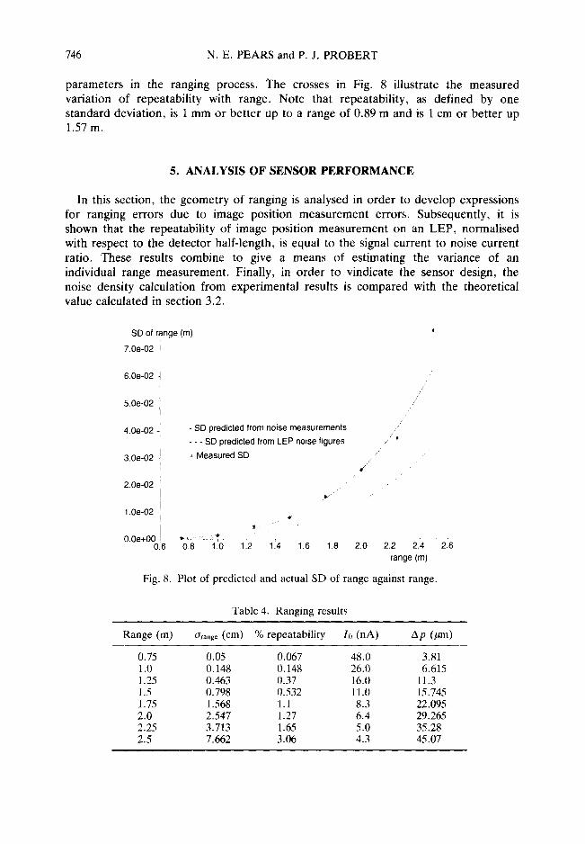
Standard deviations for all target ranges, and their values as a percentage of the target range, are shown in Table 4. In addition, the standard deviation of image position and the average detector current in nanoamps are shown. These results are used in section 5.3 to determine current noise on the LEP and intrinsic geometric

746 N . E . PEARS and P. J. PROBERT

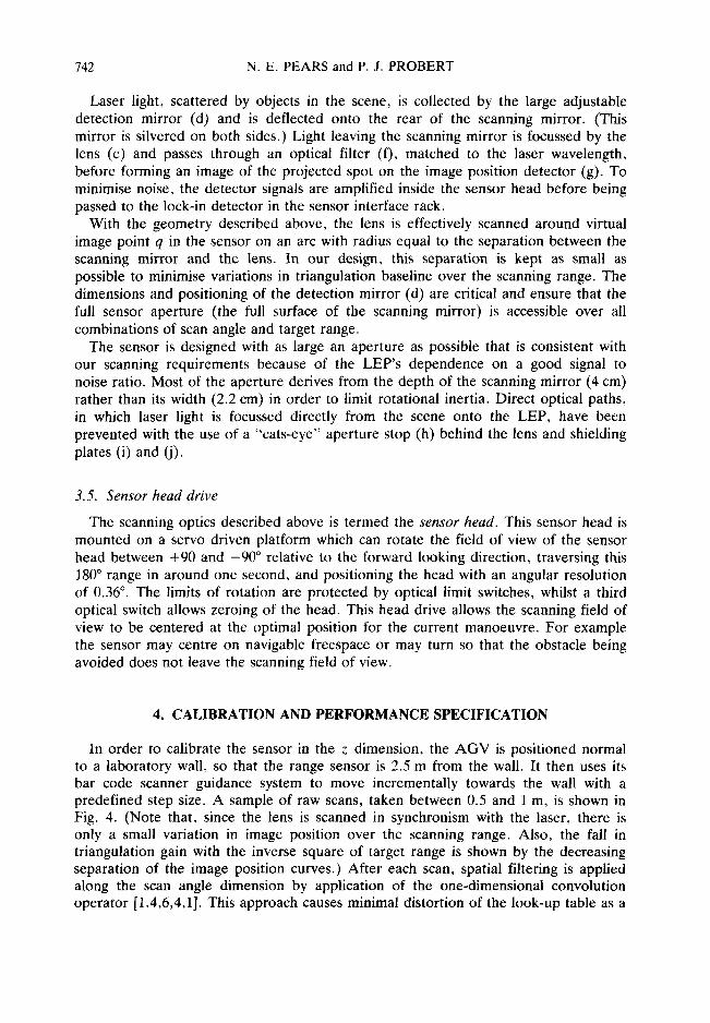
parameters in the ranging process. The crosses in Fig. 8 illustrate the measured variation of repeatability with range. Note that repeatability, as defined by one standard deviation, is 1 mm or better up to a range of 0.89 m and is 1 cm or better up 1.57 m.

5. ANALYSIS OF SENSOR PERFORMANCE

In this section, the geometry of ranging is analysed in order to develop expressions for ranging errors due to image position measurement errors. Subsequently, it is shown that the repeatability of image position measurement on an LEP, normalised with respect to the detector half-length, is equal to the signal current to noise current ratio. These results combine to give a means of estimating the variance of an individual range measurement. Finally, in order to vindicate the sensor design, the noise density calculation from experimental results is compared with the theoretical value calculated in section 3.2.

SD of range (m)

7.0e-02 1 I

6.0e-02

5.0e-02

4.0e-02 i

3.0e-02

2.0e-02 /

- SD predicted from noise measurements

- - - SD predicted from LEP noise figures

+ Measured SD

1.0e-02

i " O.Oe+O0 - , - : 0.6 0.8 1.0 1.2

?it, ~

114 1,6 1.8

: / / /

/ / t /

/ / / "

/ /

210 212 2.4 range (m)

2~e

Fig. 8. Plot of predicted and actual SD of range against range.

Table 4. Ranging results

Range (m) Orange (cm) % repeatability I0 (nA) Ap (pm)

0.75 0.05 0.067 48.0 3.81 1.0 0.148 0.148 26.0 6.615 1.25 0.463 0.37 16.0 11.3 1.5 0.798 0.532 11.0 15.745 1.75 1.568 1.1 8.3 22.095 2.0 2.547 1.27 6.4 29.265 2.25 3.713 1.65 5.0 35.28 2.5 7.662 3.06 4.3 45.07


5.1. Analysis of the ranging geometry

Figure 9 is a schematic diagram of the ranging geometry in which the range of the object is assumed to be large compared with the focal length of the collecting lens so that the focal plane is at a distance f from the principal point of the lens. Essentially, this schematic is an optical ray diagram of Fig. 3 with the laser projection axis and lens optical axis "unfolded" into their virtual image positions so that they rotate in synchronism about the origin 0 and the point q respectively. (These points correspond to the virtual positions p and q on Fig. 3.) Note that the centre of the lens does not coincide with the point q but rotates about q on an arc with radius s, the scanning mirror-lens separation.

It should be observed that, if the laser projection axis and lens optical axis were parallel, then at least half of the detector length must be unused, since a target at infinite range would project to the centre of the detector. That unused part of the detector would provide no benefit to the system in terms of depth of field or accuracy but would still contribute thermal noise to the system, thus degrading performance. The possible solutions to this problem include moving the detector off the optical axis of the lens, or introducing a vergence angle. The latter solution was chosen as the most practical, and is represented by the small angle y on Fig. 9. The analysis of this geometry, given in Appendix 1, assumes that the vergence angle is zero. Appendix 2 then modifies the equations to include this effect. This analysis yields

scene

J / a ,, f l e n s o p t i c a i axis

0 -~( /q d

Fig. 9. Geometry of the ranging process.


Z ~- f d cos2 0 P

- scos 0[1

1 + (tanO - f ) t a n

f 1 + ~ tan y

P

sec y .]

+ ----f tan y P

x = ztanO.

+ sin20 1

1 + ---f tany P

(10)

(11)

Equation (10) is expressed so that the terms in the square brackets represent the effect of the vergence angle. [Note that if ~, is zero in Eqn (10), each of the terms in square brackets is unity, which gives the result of the original analysis with zero vergence angle.]

5.2. Image position measurement performance

Rewriting Eqn (1), the image position on an LEP can be normalised with respect to the detector half-length so that

p 11 - 12 pn -- / p / / 1 + ' 2 {-1 ~ pn ~ "~1}~ (12)

\ z !

and the uncertainty in normalised position, zXpn, is given by

where

and

Ap, = 3pn AII + 3pn A12, (13) 311 312

3pn _ 212 - 212 (14) 311 (I~ + I2) 2 I~

3pn _ 211 _ 211 (15) 912 (1l + 12) 2 Io

NOW it can be shown that thermal noise in the one-dimensional LEP and the shot noise due to the dark current are significantly greater than the shot noise due to the signal current. This latter, relatively minor noise, divides between the LEP terminals according to image position. The dominant noise sources, however, divide equally between the LEP terminals. Thus, ignoring shot noise due to signal current, and denoting the remaining rms noise current by In

In A I I = AI2 - . (16)

2


Substituting Eqns (14), (15) and (16) into Eqn (13), and writing I0 for the sum of the terminal currents, gives

Ap In apo - - - - . (17)

,0

The image position repeatability is inversely proportional to the signal current to noise current ratio.

5.3. Range variance estimation

In this section, a means of estimating range error as a function of range, scan angle, and LEP detector current is developed. In general, ranging errors are dependent on image position measurement errors and scan angle errors. In the design presented here, specifications of the scanning mirror galvanometer drive indicate that ranging errors due to scan angle errors are negligible. Furthermore, if we ignore the small vergence angle in Eqn (10), and consider the dominant term only such that

z ~-" fd cos2 0, (18) P

then an estimate of the RMS value of ranging error can be computed as

Az = ~Z A p ~- z2Ap . (19) BP fd cos 2 0

Substituting for Ap using Eqn (17) gives

Az ~-

where

kz 2

I 0 COS 2 0 ' (20)

Scan angle, 0, and signal current, I0, are available each time a range measurement is made. Range itself is obtained as a function of measured image position and scan angle, through a calibration tube interpolation. Thus, to generate estimates of range variance, all that is required is to obtain an estimate of the constant, k.

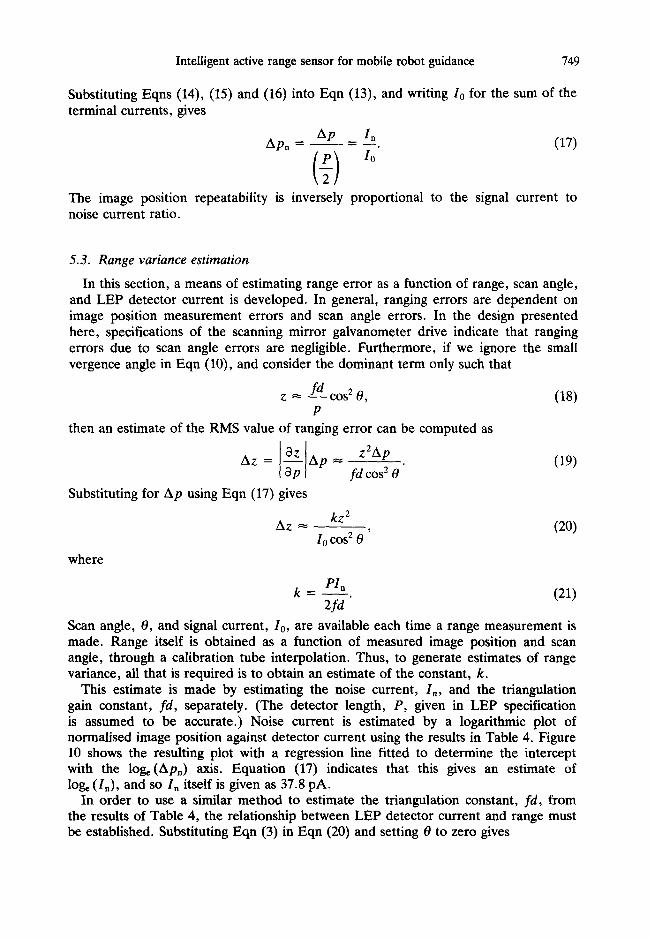
This estimate is made by estimating the noise current, In, and the triangulation gain constant, fd , separately. (The detector length, P, given in LEP specification is assumed to be accurate.) Noise current is estimated by a logarithmic plot of normalised image position against detector current using the results in Table 4. Figure 10 shows the resulting plot with a regression line fitted to determine the intercept with the loge(Apn ) axis. Equation (17) indicates that this gives an estimate of loge (In), and so I~ itself is given as 37.8 pA.

In order to use a similar method to estimate the triangulation constant, fd , from the results of Table 4, the relationship between LEP detector current and range must be established. Substituting Eqn (3) in Eqn (20) and setting 0 to zero gives

k - (21) 2fa


-16.5

-17

i -17.5

g

E_ - t8

8 -t8.5

- 1 9

+• regression gradient = -0.98

\ Iog(n.Lr) intercept = -24.0

- 1 9 . 5 J ~ ~ - - - - ~ - 7 . 5 - 7 - 6 . 5 - 6 - 5 , 5 - 5 - 4 .

Iog(Io)

Fig. i0. Logarithmic plot of Ap against signal current.

where

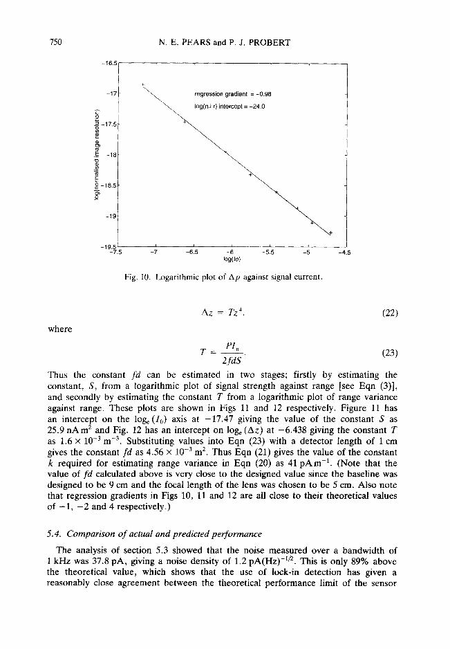
A z = T z 4 , (22)

T - PIn (23) 2fdS

Thus the constant fd can be estimated in two stages; firstly by estimating the constant, S, from a logarithmic plot of signal strength against range [see Eqn (3)], and secondly by estimating the constant T from a logarithmic plot of range variance against range. These plots are shown in Figs 11 and 12 respectively. Figure 11 has an intercept on the log e(I0) axis at -17.47 giving the value of the constant S as 25.9 n A m 2 and Fig. 12 has an intercept on log~ (Az) at -6.438 giving the constant T as 1.6 x 10 -3 m -3. Substituting values into Eqn (23) with a detector length of 1 cm gives the constant fd as 4.56 × 10 -3 m 2. Thus Eqn (21) gives the value of the constant k required for estimating range variance in Eqn (20) as 41 pAre -1. (Note that the value of fd calculated above is very close to the designed value since the baseline was designed to be 9 cm and the focal length of the lens was chosen to be 5 cm. Also note that regression gradients in Figs 10, 11 and 12 are all close to their theoretical values of - 1 , - 2 and 4 respectively.)

5.4. Comparison of actual and predicted performance

The analysis of section 5.3 showed that the noise measured over a bandwidth of 1 kHz was 37.8 pA, giving a noise density of 1.2 pA(Hz) -1/2. This is only 89% above the theoretical value, which shows that the use of lock-in detection has given a reasonably close agreement between the theoretical performance limit of the sensor

-16.5 - - - -

-17

-17.5

~ regression gradient = -2.02

~ og(n.i.r) intercept = -17.47

_s" -18

o

-18.5

-19

InteUigent active range sensor for mobile robot guidance 751

-19.5 ~ i ~ ~ , L -0.4 -0.2 0 0.2 0.4 0.6 08

log(z)

Fig. 11. Logarithmic plot of signal current against range.

-2

-3

- 4

"5 o

~ - - 5

-6

-7

-8 -0.4

+

regression gradient = 4.06 + ~ . . + = - - .

-012 0 01.2 0.4 01.6 0.8 log(z)

Fig. 12. Logarithmic plot of Az against z.

and its actual ranging performance. The ranging repeatability predicted from this theoretical noise density by projecting the resulting theoretical image position repeatability through the estimated triangulation gain is shown by the dashed line on Fig. 8. The solid line shows the expected performance using the measured values of noise density and triangulation gain.


6. INTEGRATION OF THE SENSOR INTO THE LICA ARCHITECTURE

6.1. System overview

In addition to underpinning the LICA architecture, transputer technology provides simple interfacing to external sensing and actuating devices via readily available commercial link adaptors such as the C O l l . This is essential given that the physical manifestation of robotic systems is an assembly of sensing and actuating devices with which it interacts with the real world.

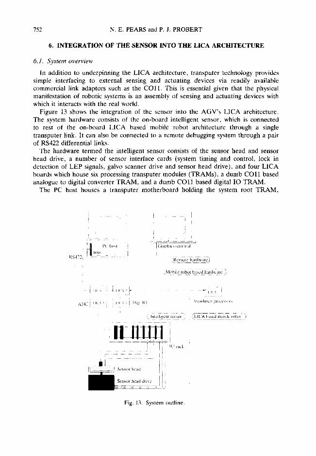
Figure 13 shows the integration of the sensor into the AGV's LICA architecture. The system hardware consists of the on-board intelligent sensor, which is connected to rest of the on-board LICA based mobile robot architecture through a single transputer link. It can also be connected to a remote debugging system through a pair of RS422 differential links.

The hardware termed the intelligent sensor consists of the sensor head and sensor head drive, a number of sensor interface cards (system timing and control, lock in detection of LEP signals, galvo scanner drive and sensor head drive), and four LICA boards which house six processing transputer modules (TRAMs), a dumb C O l l based analogue to digital converter TRAM, and a dumb C O l l based digital IO TRAM.

The PC host houses a transputer motherboard holding the system root TRAM,

t , J,(' ho.t [6,~,i, hi~, ~-~.-,,,,i,,,--~-

k S 4 2 2 Rt ' l l l t)[~. ' h a r d w a i ' c

N 4 o b l l c r o b o t b a > , c d h : l r t l ' , , , t l r c ',

A I ) ( ' . .t ~. ~ i ii .~ . [ )1~ l( ) ~ \ t ioa fwt2 l')r(),:t_',,,~oi,

h l lc l ! lgc! l_ t ~t . 'nst ,!_ I . I C A b a s e d n ) t )b ] l e r o b o t

ilJnIn

S e n s o r h e a d drP, 'L ' . [ J

Fig. 13. System outline.


which configures the system and provides debugging facilities, and a graphics TRAM, which provides a real-time display of the range scans. If debugging and graphics are not required the RS422 umbilical cord can be disconnected and the remaining transputers can be booted from EPROM.

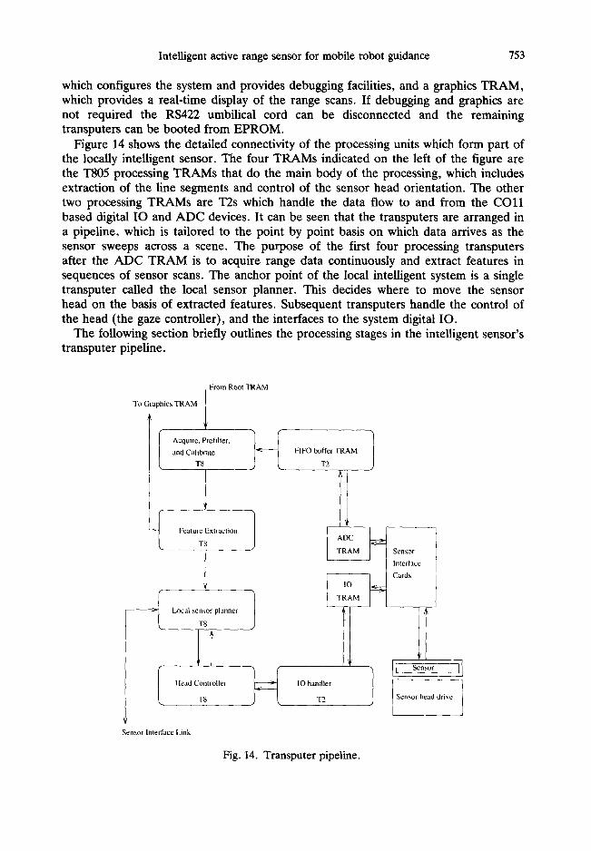
Figure 14 shows the detailed connectivity of the processing units which form part of the locally intelligent sensor. The four TRAMs indicated on the left of the figure are the T805 processing TRAMs that do the main body of the processing, which includes extraction of the line segments and control of the sensor head orientation. The other two processing TRAMs are T2s which handle the data flow to and from the C O l l based digital IO and ADC devices. It can be seen that the transputers are arranged in a pipeline, which is tailored to the point by point basis on which data arrives as the sensor sweeps across a scene. The purpose of the first four processing transputers after the ADC TRAM is to acquire range data continuously and extract features in sequences of sensor scans. The anchor point of the local intelligent system is a single transputer called the local sensor planner. This decides where to move the sensor head on the basis of extracted features. Subsequent transputers handle the control of the head (the gaze controller), and the interfaces to the system digital IO.

The following section briefly outlines the processing stages in the intelligent sensor's transputer pipeline.

From Root TRAM

To Graphics TRAM

and Calibrate. FIFO buffer TRAM T8 T2

FeatureTSEXtraction 1

-i Local sensor planner |

J "1"8

I lead Controller

1"8

t

IO handler

T2

Sensor Interface Link

Fig. 14. Transputer pipeline.

Sensor t Interface Cards

Sensor

1 Sensor head drive [ ]


6.2. The transputer pipeline

6.2.1. Data acquisition and buffering. Sensor data enters the T R A M network synchronously at 2.5 kHz, by externally triggering A to D conversion of the amplified and demodulated LEP terminal signals on the sensor's system clock. The A D C TRAM sends the data along a transputer link to a FIFO buffering T R A M as it is converted, which removes synchrony at the front end of the pipeline, and so relaxes timing constraints. This means that the maximum scan rate, as defined by pipeline processing limitations, depends on the average time to process a point, and nct the maximum time to process a point.

6.2.2. Filtering and range mapping. The subsequent T R A M requests data from the FIFO buffer and calculates normalised image position, with which there is an associated scan angle, detector current and sensor head angle. Any image positions registered outside the calibration range for a given angle are ignored. Also, range positions registered with low detector current are rejected in accordance with a dynamic threshold. This threshold requires a predefined minimum detector current at the defined minimum range, I z"'° and readings are rejected for which

0mi n '

- Z 2

Effectively, this dynamic signal threshold filters out areas of poor reflectivity, since it is in the same form as the inverse square law of signal strength with range. In particular, the dynamic threshold is effective in filtering out those noisy range readings at edges, which are associated with the (near) zero signal current of missing parts. Such areas, which can be thought of as having zero reflectivity, can be rejected at close ranges without blanking out measurements which are of low signal strength due to their larger range. For the remaining points, the sensor calibration described in section 4 provides the mapping

(p, 0P) T--, (z, x) r (25)

Also, before each data point is passed to the feature detection TRAM, an associated range variance is calculated, as described in section 5.3.

6.2.3. Range discontinuity detection. It is assumed that the range data set for a given scan can be associated with a piecewise linear model of the world. If the parameters of such a model can be extracted from a scan, they can be used to guide both sensor head movements and vehicle movements in a purposeful, task-oriented manner. For many real environments in which autonomous vehicles operate (contain- ing, for example, walls, pillars and boxes), a piecewise linear assumption is not unrealistic. Parts of the environment where the assumption does not hold can be identified because the discontinuities extracted will not exhibit predictable behaviour when the vehicle and sensor head move.

The feature extraction algorithm must estimate the parameters of the line segments, the position of range discontinuities, and their associated uncertainties. The standard least squares estimator is inappropriate, since the world coordinates x and z are not independent, but are related by Eqn (11). Also, the algorithm must cater for sensor head movements, since they can be significant in the time it takes for a single scan.


The Extended Kalman Filter (EKF) satisfies these requirements and provides a computational framework in which sensor head movements are catered for by the evolution of an appropriate state. This algorithm is recursive and so maps very well onto a point by point pipelined transputer architecture. The advantage of this approach is that edges are found with minimal latency as the sensor scans across the scene. Typically this latency is two to three range sample periods, or around 1 ms, which compares favourably with a batch processing approach which must incur delays of more than 256 range sample periods, or around 100 ms.

The edge position information is employed both by the intelligent sensor itself to control the sensor field of view and at the tactical level of the robot navigation system for obstacle avoidance and docking.

6.2.4. Local sensor planner. The local sensor planner implements a finite state machine, where each state is a particular sensor head behaviour. State sequencing is dependent on the type of manoeuvre, the current state, and the local sensor observations provided by the line segment extraction algorithm. Currently, these states include the following.

• Slaving the head orientation to the tangent of the vehicle path. • Centering on the nearest discontinuity (edge) in the vehicle frame. • Moving the head so that it is parallel to a line segment. • Centering on freespace.

The first of these is the default state, reflecting the fact that the sensor should "look" in the direction that the vehicle is moving. The other three states operate when a potential collision is detected, each one defining a different way in which the sensor head should move on the basis of the line segments extracted from the most recent scan.

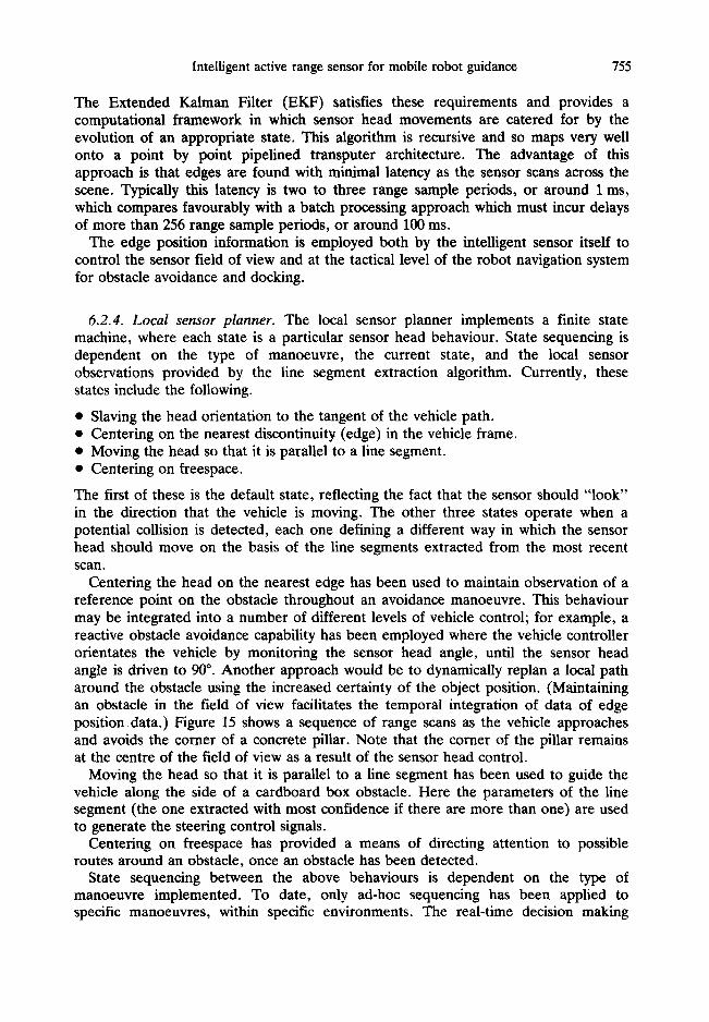
Centering the head on the nearest edge has been used to maintain observation of a reference point on the obstacle throughout an avoidance manoeuvre. This behaviour may be integrated into a number of different levels of vehicle control; for example, a reactive obstacle avoidance capability has been employed where the vehicle controller orientates the vehicle by monitoring the sensor head angle, until the sensor head angle is driven to 90 °. Another approach would be to dynamically replan a local path around the obstacle using the increased certainty of the object position. (Maintaining an obstacle in the field of view facilitates the temporal integration of data of edge positiondata.) Figure 15 shows a sequence of range scans as the vehicle approaches and avoids the comer of a concrete pillar. Note that the comer of the pillar remains at the centre of the field of view as a result of the sensor head control.

Moving the head so that it is parallel to a line segment has been used to guide the vehicle along the side of a cardboard box obstacle. Here the parameters of the line segment (the one extracted with most confidence if there are more than one) are used to generate the steering control signals.

Centering on freespace has provided a means of directing attention to possible routes around an obstacle, once an obstacle has been detected.

State sequencing between the above behaviours is dependent on the type of manoeuvre implemented. To date, only ad-hoc sequencing has been applied to specific manoeuvres, within specific environments. The real-time decision making


1.5m

Fig. 15. Centering a corner by sensor head control.

0.Sin

required for effective active sensor control in a more general sense is not addressed here, though the active sensor provides a useful tool for implementing and evaluating such schemes.

6.2.5. Sensor head position controller. Demand sensor head positions are passed to the head position controller from the sensor planner TRA M at the scan rate, 9.8 Hz. This controller is a synchronous process in which a sensor scan time interval is divided into 10 control time intervals. An appropriate demand velocity is computed and output to the head motor control board at each of these control time intervals.

7. CONCLUSIONS

The mechatronic design of a range sensor, the characterisation of its performance, its integration into a mobile robot architecture, and the processing required to actively control its field of view have been described. Low noise preamplifier design and lock-in detection gave a measurement system with a noise figure close to the theoretical one based on the LEP specifications. This low noise performance has extended the application domain of LEPs to larger depths of field whilst still using a laser power which is eye safe.

Analysis of LEP image position measurement and a geometric model of the ranging process have allowed meaningful algorithms to be applied to the range data. In particular, the LEP based sensor has the useful properly of a Gaussian noise form of image position measurement, the variance of which can be accurately estimated from signal intensity. Thus the sensor has been amenable to line segment extraction using an algorithm based on the Extended Kalman Filter.

The sensor has proved to be suitable for guiding close range real-time mobile robot manoeuvres because it is optically based (and therefore can provide a high spatial density of range readings), fast, accurate, it has a wide field of view, and is active and locally autonomous. The senor is a locally autonomous agent which has been, and continues to be, a useful platform with which to investigate the interaction between active sensor control (sensor planning) and vehicle control for close range mobile robot manoeuvres.


R E F E R E N C E S

1. Hu H., Sensor-based control architecture. In Advanced Guided Vehicles (Edited by Cameron S. and Probert P.), Series in Robotics and Automated Systems, Ch. 3, p. 17-35. World Scientific Publishing, Singapore (1994).

2. Pollard S. B., Mayhew J. E. W. and Frisby J. P., PMF: a stereo correspondence algorithm using a disparity gradient. Perception 14, 449-470 (1985).

3. Harris C., Geometry from visual motion. In Active Vision (Edited by Blake A. and Yuille A.). MIT Press, Cambridge, MA (1992).

4. Jarvis R. A., A perspective on range finding techniques for computer vision. IEEE Trans. Pattern Anal. Mach. Intell. 5,122-139 (1983).

5. Everett H. R., Survey of collision avoidance and ranging sensors for mobile robots. Robotics Auton. Syst. 5, 5-67 (1989).

6. Miller G. L. and Wagner E. R., An optical rangefinder for autonomous robot cart navigation. In Mobile Robots H, SPIE 852, pp. 132-144, Cambridge, MA, 5-6 November. Bellingham, Washington (1987).

7. Kuc R., A spatial sampling criterion for sonar obstacle detection. IEEE Trans. Pattern Anal. Mach. Intell. 12(7), 686-690 (1990).

8. Reid G. T. and Rixon R. C., Stripe scanning for engineering. Sensor Review 8(2), 67-71 (1988).

9. Lo H. R., Blake A., McCowen D. and Konash D., Epipolar geometry for trinocular active range sensors. In Proc. British Machine Vision Conf., pp. 19-24, Oxford, 24-27 September (1990).

10. Pears N. E. and Probert P. J., Active triangulation rangefinder design for mobile robots. In Proc. IEEE/RSJ Int. Conf. on Intelligent Robots and Systems, volume 3, pp. 2047-2052, Raleigh, NC, 7-10 July (1992).

11. Pears N. E. and Bumby J. R., Guidance of an autonomous guided vehicle using low-level ultrasonic and odometry sensor systems, lEE Trans. Inst. Meas. Control 11(5), 231-248 (1989).

12. Pears N. E. and Probert P. J., An optical range sensor for mobile robot guidance. In Proc. IEEE Int. Conf. on Robotics and Automation, volume 3, pp. 659-665, Atlanta, GA, May (1993).

13. Livingstone F. R. and Rioux M., Development of a large field of view 3-d vision system. In Optical Techniques for Industrial Inspection, SPIE 665, pp. 188-194, Quebec City, 4-6 June. BeUingham, Washington (1986).

A P P E N D I X 1: G E O M E T R I C A N A L Y S I S OF T H E S E N S O R

In the geometric analysis of the ranging process, it is assumed that the optical centre of the lens is scanned about a point, q, which is at the same z coordinate as the origin of the laser scan, 0, as shown in Fig. 9. The sensor was designed so that this would be the case to a good approximation.

Assume, initially, that the small vergence angle, y, is zero, then examination of Fig. 9 reveals the following three relationships.

x - d + a - tan(0 - q~) (A1)

Z

tan 0 - x (A2) Z


From Eqns (A1) and (A2)

tan 0 - p . (A3) f

d - a - - - tan 0 - tan (0 - (p). (A4)

Z

Expanding the tangent of a sum gives

d - a _ tan0(1 + t a n 20) (A5)

z 1 + tan 0 tan q~

Substituting for tan q~ using Eqn (A3) and rearranging gives

f c o s 2 0 ( 1 + P - - - t a n 0 ) ( d - a ) f

z = (A6) P

The length, a, shown in Fig. 9 varies with both scan angle, 0, and the angular displacement associated with the image position, q~. Applying the sine rule to the triangle bounded by a, s and the detection axis in Fig. 9 gives

a - s sin (P . (A7) cos (0 - q~)

Expanding the cosine of a sum and rearranging gives s

a = . (A8) cos 0(cot q) + tan 0)

Substituting the above equation into Eqn (A6) and rearranging gives

z = f d cos2 0 + __d sin20 - s cos 0. (A9) p 2

Note that the effect of the lens-mirror separation is equal to the length of that separation resolved in the z direction, as expected.

APPENDIX 2: THE EFFECT OF VERGENCE ANGLE

With the addition of a vergence angle, y, Eqn (A1) becomes

x - d + a - t a n ( 0 - q~- 7),

z whereas Eqns (A2) and (A3) remain intact. Thus we have

d - a _ t a n 0 _ t a n ( 0 - y ) - tan z 1 + t a n ( 0 - y) tanq~

Substituting for tan ~ using Eqn (A3) and rearranging gives

t an0 - tan(0 - y) + P ( t a n 0 t a n ( 0 - y) - d a J

Z 1 + P - - - t a n ( 0 - y)

f

1)

(A10)

( A l l )

(A12)


but, from the tangent of a sum we have

t a n O - t a n ( O - 7) =

and

tan 7(1 + tan 2 0) 1 +tan0tan7

(A13)

tan 0 tan (0 - 7) = tan2 0 - tan 0 tan Y (A14) 1 + tan 0 tan 7

Also, with a vergence angle included, Eqn (A8) becomes S

= . (A15) a cos(0 - 7)(cot ¢ + tan(0 - 7))

Substituting Eqns (A13)-(A15) into Eqn (A12) and rearranging gives

[ l+( tan0-__ tany] z = f d COS2 0 . . . . . . ~ .

P 1 + ]---tan7

P

I 1 l _ s c o s 0 [ secTf / ]" (AI6) dsin20 +

1 + ), 1 + p t a n T j 2 f tan P

Note that if 7 is zero, then each term in square brackets is unity, and we have the same result as was derived with zero vergence angle.

an intelligent active range sensor for … local processing provides greater autonomy, ... the...

Documents