1

An Integrated Sampling and Quantization Schemefor Large-Scale Compressive Reconstruction

Zhao Song∗, Andrew Thompson†, Robert Calderbank∗, and Lawrence Carin∗

Abstract—We study integrated sampling and quantizationstrategies for compressive sampling, and compressive imaging inparticular. We propose a novel regionalized non-uniform scalarquantizer, which adaptively assigns different bit budgets to dif-ferent regions. The bit assignment task is formulated as a convexoptimization problem which has an exact closed-form solution,under certain conditions. The method gives improved quantiza-tion error compared to the scalar quantizers typically used incompressing sampling, while offering considerable computationaladvantages over typical vector quantization approaches. We alsodesign fully deterministic sampling matrices whose performanceis robust to the rejection of saturated measurements, and whichpermit the efficient encoding of rejected measurements. Wepresent fast transforms for computing matrix-vector productsinvolving these sampling matrices. Our experiments show thatboth our sampling and quantization schemes outperform otherstate-of-the-art methods while being scalable to large imagereconstruction problems.

I. INTRODUCTION

The past decade has witnessed the rapid development ofcompressive sampling (compressed sensing), since the pio-neering work of Candes et al. [1] and Donoho [2]. Theresearch community has focused on the important special caseof reconstruction of a sparse signal from an underdeterminedlinear system. More recent work has addressed the practicallyrelevant problem of reconstruction from quantized compres-sive samples [3, 4, 5, 6, 7, 8, 9, 10, 11].

Uniform scalar quantization (USQ) [12] is often used in acompressive sampling context due to ease of implementationand analysis [4, 5, 6, 9]. A uniform scalar quantizer wasproposed in [8] which aims to optimize the distortion of thereconstructed signal as opposed to the measurements. In [10],a non-uniform quantizer was derived which minimizes thereconstruction error within a message passing framework, byusing of a state evolution analysis. Both of these approachesassume a restrictive signal model, and in addition the latterrequires a sequential quadratic programming (SQP) method tosolve the underlying optimization problem and therefore doesnot scale easily to large problems.

Scalar quantization is an example of quantization democ-racy [13], the principle that individual bits in a quantizedrepresentation of a signal receive equal weight in approximat-ing the signal. However, as was argued in Kostina et al. [7],democratic (scalar) quantization is suboptimal for compressive

∗Z. Song, R. Calderbank, and L. Carin are with the Department of Electricaland Computer Engineering, Duke University, USA; email: zhao.song,robert.calderbank, lcarin@duke.edu†A. Thompson is with the Mathematical Institute, University of Oxford,

UK; email: thompson@maths.ox.ac.uk

sampling due to the geometrical properties of commonlyused sampling matrices. For example, improvements are tobe expected by allowing the bit budget allocation to varyover the measurement distribution. Vector quantizers adaptedto compressive sampling have been proposed; for example,a joint source-channel vector quantization scheme for com-pressive sampling was developed in [14]. The computationalcomplexity is high, however, and the application to large-scale problems such as image reconstruction is not addressed.There is a need for quantizers for compressive measurementswhich give improved performance over scalar quantizationwhile reducing the complexity of typical vector quantizationmethods.

A further issue, often neglected, is whether to allow mea-surements to exceed the dynamic range of the quantizer,typically referred to as saturation. The naıve approach is tochoose the dynamic range to be suitably large enough thatsaturation hardly ever occurs. Laska et al. [5], on the otherhand, proposed two strategies in which a nontrivial proportionof measurements are allowed to saturate. One approach isto build the assumption of saturated measurements into theoptimization problem in the form of additional constraints.The other approach, which we choose to adopt and furtherdevelop in this paper, is to simply reject the measurementswhich exceed the chosen dynamic range. It was demonstratednumerically in [5] that this apparently wasteful strategy ofthrowing away information can improve the accuracy of signalrecovery. Theoretical guarantees of robust signal recoverywere also obtained in [5] provided the sampling matrix satis-fies a restricted isometry property (RIP) [15] after the removalof rows corresponding to the rejected measurements. Theauthors reinterpret this property as a measure of measurementdemocracy, the notion that each measurement contributes asimilar amount of information about the underlying signal inthe compressed representation.

Kostina et al. [7] extended the work of [5] by proposinga new framework for evaluating computational efficiency, inwhich the number of bits needed to encode the indices of therejected measurements is taken into account. To mitigate thisextra overhead, the authors proposed the use of deterministicDelsarte-Goethals frames in which only a sub-collection ofstructured sets of measurements are allowed as candidatesfor rejection. Numerical experiments in [7] showed that theirdeterministic rejection scheme led to improvements in quan-tization error. The reason for the improvement is that moreefficient encoding of the rejected indices means that a finergrid can be imposed on the remaining measurements for thesubsequent quantization.

2

This paper proposes practical and computationally efficientstrategies for quantized compressive sampling, which scalewell to high-dimensional problems that occur, for example, inimage reconstruction. We design deterministic sampling ma-trices for rejection-based quantization for which the rejectedmeasurements can be efficiently encoded, and which have twoproperties crucial for incorporation into practical compressivesampling schemes, namely• they have compressive reconstruction properties which

are robust to rejection;• their associated matrix-vector products can be computed

using fast transforms.We also propose a regionalized scalar quantizer which• improves both quantization and reconstruction error com-

pared to standard scalar quantization;• has significantly reduced computational complexity com-

pared to vector quantization methods.By addressing together the inter-related issues of how tosample and how to quantize, we propose a practical, integrated,solution to quantized compressive sampling.

More specifically, our two main contributions are as follows.1) Following the broad approach of [7], we show how to

construct fully deterministic sampling matrices basedon Delsarte-Goethals frames which are appropriate forrejection-based quantization. We also present provablyfast transforms for performing their associated matrix-vector products, a crucial requirement for tractable/fastrecovery algorithms. Our constructed matrices havenear-optimal coherence, which is a property known toimprove the fidelity of reconstruction methods based onconvex optimization [16, 17]. Moreover, the matricesconsist of stacked row blocks and are designed so thatthe removal of row blocks results only in a controlleddeterioration of the matrices’ coherence, thereby makingthem robust to rejection. Inspired by [7], we then opti-mize the rejection with respect to a reduced number ofrow block combinations, indexed using a binary finitefield. We compare our proposed sampling scheme toGaussian matrices and demonstrate that we can recoverthe underlying signal more accurately from quantizedsamples using our scheme.

2) We propose a novel regionalized non-uniform scalarquantization scheme which is able to adapt to unknownmeasurement distributions. Our method is based onoptimizing an upper bound on the quantization errorfunction. We show that that this surrogate optimizationproblem is convex, and that it has a closed-form solution.We assign different bit budgets to different regions tomatch their distribution; within each region, we applyLloyd’s algorithm [18] to generate the quantization level,as a fine-tuning step. Experiments on natural imagesshow that this regionalized non-uniform scalar quantizerconsistently outperforms state-of-the-art scalar quantiz-ers in terms of quantization error, and state-of-the-artvector quantizers in terms of computational efficiency.

We note that two different notions of democracy [13, 5]play an important role in the design of quantizers for compres-

sive reconstruction. Effective compressive sampling matricestypically enjoy the property of measurement democracy, whilethe performance/efficiency trade-off between scalar and vectorquantization methodologies can also be viewed in terms ofquantization democracy. In this paper we propose a democraticsampling scheme which is also practically implementable andamenable to structured rejection, and a quantization schemewhich is only partially (regionwise) democratic. A naturalextension would be to consider combining our approachwith the non-democratic multi-level sampling schemes oftenespoused for compressive imaging [19, 20, 21], but we leavethis interesting extension as future work.

The structure of the rest of the paper is as follows. Section IIprovides a broad overview of our general framework. Wepresent our sampling matrix construction in Section III. Wethen show in Section IV how to design the regionalizedquantizer. Section V provides our experimental results, andSection VI concludes the paper.

II. OVERVIEW OF OUR FRAMEWORK

A. Rejection-Based Quantization Scheme

Before presenting in detail our sampling and quantizationschemes, we first outline in broad terms a framework forsignal reconstruction from quantized samples using structuredrejection [7].

1) Obtain the original measurement y ∈ RN as y = Ax+ε, where A ∈ RN×p is the sensing matrix designedin Section III, x ∈ Rp is the underlying signal to bereconstructed, and ε ∈ RN is an arbitrary noise vector.

2) Fix a collection Ω of index sets corresponding to rejec-tion sets of cardinality D.

3) Reject the measurements indexed by the set ω ∈ Ω withmaximal `2-norm, i.e.,

ω = arg maxω∈Ω‖yω‖2.

4) Collect the surviving measurements y ∈ RN−D as

y = y[1:N ] \ ω. (1)

Equivalently, we obtain the sensing matrix A by remov-ing from A the rows whose indices are contained in ω.

5) Quantize y to obtain y as y = Q(y) using the region-alized nonuniform quantizer described in Section IV.

6) Use y and A in a compressive sensing recovery algo-rithm to reconstruct the signal x.

Note that the key idea here is that after the rejection stepin (1), a finer grid can be put on the surviving measurementsfor the subsequent quantization step. Unlike Laska et al. [5],this framework avoids the difficult task of tuning the saturationlevel when rejecting measurements. Moreover, in contrastto Laska et al. [5], here we take a realistic account of the totalnumber of bits required, comprising those required to encodethe rejection indices in Ω, describe the quantization region andperform the quantization itself. Given a budget of τN bits,we need to distribute this total among encoding the rejectionindices, encoding the quantization region, and encoding theindividual quantization levels.

3

B. Design Motivation

In this paper and much previous work [3, 4, 5, 6, 7, 8, 9,10, 11], quantized compressive sensing can be represented asthe following unconstrained optimization problem, which hasa similar form to the basis pursuit denoising (BPDN) [22]problem.

minimizex∈Rp

‖y − Ax‖22 + λ ‖x‖1 (2)

where y and A are defined in Section II-A. We notice thatthe objective function in (2) can be upper bounded by twoseparate terms, namely the quantization error and the BPDNobjective, as shown in Lemma 1.

Lemma 1. The objective function of quantized compressivesensing in (2) is upper bounded as

‖y−Ax‖22 +λ ‖x‖1 ≤ ‖y − y‖22︸ ︷︷ ︸quantization error

+ ‖y − Ax‖22 + λ ‖x‖1︸ ︷︷ ︸BPDN objective

Proof: Applying the triangle inequality on the objectivein (2) leads to the conclusion.

Lemma 1 suggests that the original problem in (2) can bedecomposed into two sub problems: reducing the quantizationerror and solving the original BPDN. By minimizing bothterms separately, we can achieve a smaller upper bound ofthe objective in (2). In Section III we concentrate on mini-mizing the reconstruction error: we develop novel structuredsampling matrices whose coherence properties are robust toremoval of row blocks. In Section IV, we focus on minimizingquantization error: we design a regionalized non-uniformscalar quantizer which achieves improved quantization errorscompared to several other widely used quantization schemes.

III. DESIGN OF A STRUCTURED SENSING MATRIX

Our construction employs Delsarte-Goethals (DG) frames,which have been previously proposed for compressive sam-pling in Calderbank et al. [23] and Duarte et al. [24], andwhich have been shown empirically to allow reconstructionperformance indistinguishable from that of Gaussian matri-ces in the case of uniform (unstructured) sparsity and `1-minimization decoding [25]. We consider one particular in-stantiation of DG frames known to have near optimal coher-ence: real Kerdock matrices1. Fix a positive integer m, andindex the rows of a matrix K of dimensions 2m+1 × 22m+1

by v =[vm+1 . . . v2 v1

]T, a binary string of length

m + 1, for which we write v ∈ Fm+12 , where F2 is the

binary finite field. Similarly, index the columns of K by[aT bT

]T, where a =

[am . . . a2 a1

]T ∈ Fm2 andb =

[bm+1 . . . b2 b1

]T ∈ Fm+12 (binary strings of length

m and m + 1 respectively). Define the entries of K to beexponentiated Kerdock codes, namely

Kv,(a,b) := (−1)bT v+ 1

2 vTRav, (3)

1Delsarte-Goethals frames are complex, but real analogues can be obtainedfrom them by applying a Gray mapping to codes which generate the complexframes, see [24, Appendix B] for more details.

whereRa :=

[0 aT

a Qa + aaT

], (4)

and where Qa ∈ Km = Qa : a ∈ Fm2 such thatdiag(Qa) = a, and where Km is a Kerdock set of 2m binarym×m Hankel matrices. The set Km has the property that thedifference between any two distinct elements of the set is fullrank2. It can also be shown that the matrix K is a union of2m orthonormal matrices of size 2m+1 × 2m+1, namely

K =[D0Hm |D1Hm | . . . |D2mHm

], (5)

where Hm is the 2m+1 × 2m+1 Hadamard matrix withrows/columns in standard (Hadamard) order, and each Di isa diagonal matrix whose diagonal entries are (−1)

12vTRav for

some a. We note that the factor of number of columns torows is high: 2m. For practical applications it is common totruncate the matrix to obtain the desired undersampling ratio.Our constructions will in fact involve two Kerdock codes:an “inner” and an “outer” code. The inner code will not betruncated, but the outer code will be truncated according tothe desired undersampling ratio.

1) Construction 1: “Stacked Kerdock” matrix: We build anorthogonal matrix M by stacking Kerdock row blocks. Moreprecisely, we introduce another binary string u ∈ Fm2 to indexthe row blocks, and define

M(u,v),(a,b) := 2−(2m+1)

2 (−1)aTu+bT v+ 1

2 vTRav. (6)

A proof that M is orthogonal is given in Appendix A. Theconstruction of M constitutes the “inner code”, and it isdesigned to be robust to the removal of row blocks. Now weuse M to form a new “Kerdock-like” matrix by replacing theHadamard matrix H2m+1with M . We thus generate diagonalmatrices E1, E2, . . . , Er, where r ≤ 22m using the Kerdockset K2m, the “outer code”, giving

A =[E1M |E2M | . . . |ErM

]. (7)

Note that the dimensions of A are 22m+1× r · 22m+1, givingan undersampling ratio of 1/r.

2) Construction 2: “Permuted Hadamard” matrix: Wefollow the same approach as for Construction 1, except thatwe make a change to the definition of the matrix Ra, replacing(4) by

Ra :=

[0 aT

a Qa + diag(a)

]. (8)

The expression in (8) differs from (4) in just one term, andalso ensures that the quadratic form 1

2vTRav is well-defined

and integer. With this small change, the matrix M is nothingother than a Hadamard matrix with permuted rows, which wenext demonstrate. For each v ∈ Fm+1

2 , define rv ∈ Fm2 to bethe binary vector satisfying

(rv)i :=1

2vTReiv,

where ei is the vector with a one in position i and zerootherwise. Then it is easy to show that 1

2vTRav = aT rv and,

2The matrix Ra is a Hankel matrix with zeros on its diagonal, which issufficient to ensure that the quadratic form 1

2vTRav is an integer and thus

(3) is well defined.

4

after substitution into (6) and a little rearrangement, we arriveat

M[u v],[a b] := 2−(2m+1)

2 (−1)aT (u+rv)+bT v, (9)

from which it follows that M is a Hadamard matrix H2m+1

with rows permuted as

σ :

[uv

]→[u+ rvv

].

That σ is a permutation is clear on observing that it is aself-inverse mapping from F2m+1

2 to itself. M is triviallyorthogonal since it is a row-permuted Hadamard matrix. Wethen use the new M to build the matrix A in the same wayas for Construction 1.

3) Coherence measures: Define the coherence µ(A) of amatrix A to be the maximum normalized inner product ofany two distinct columns of A. In other words, writing A =[a1 a2 . . . ap

],

µ(A) := maxi 6=j

|aTi aj |‖ai‖2‖aj‖2

. (10)

It has been shown that a sufficient condition for recoveryof a vector of sparsity k using `1-minimization is that thesensing matrix A satisfies µ(A) < 1/(2k − 1)[16, 17] and,since an N × p Kerdock matrix has coherence 1/

√N for

N an even power of 2 and 2/√N for N an odd power

of 2, vectors of sparsity of the order√N are guaranteed

to be recovered. Coherence is not a necessary condition forgood compressive sampling performance, which is typicallyobserved to be better in practice in the case of Kerdock (andmany other) matrices, with k proportional to N rather than√N . Nonetheless, coherence is still often a reliable guide to

the performance of a matrix in compressive sampling and ametric highly relevant to the successful design of a samplingmatrix. In particular, we wish to design sensing matrices whosecoherence deteriorates in a robust manner when row blocks areremoved from it.

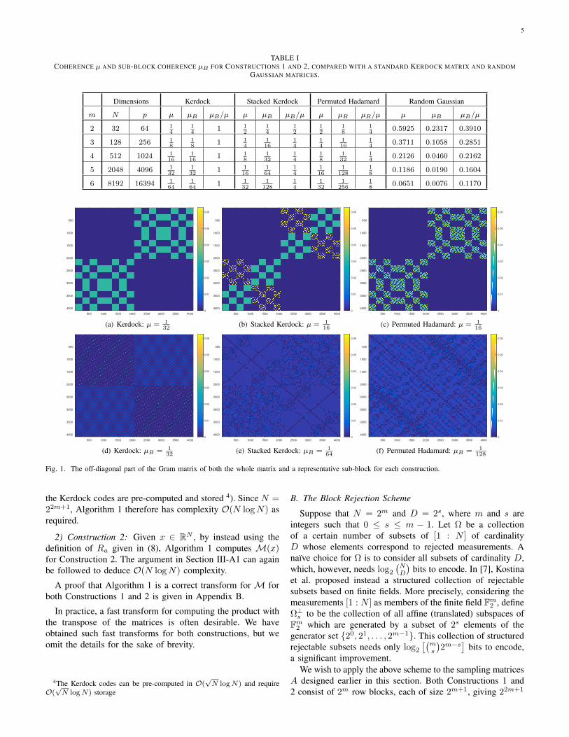
First we investigate the coherence of the whole matrix. Weconsider matrices of different dimensions, with two blocksin the outer Kerdock code, giving an undersampling ratio of1/2. In terms of the parameter m, the matrices thus havedimensions 22m+1×22m+2. We compare Constructions 1 and2 with an obvious baseline, namely a standard (outer) Kerdockmatrix. Table I gives coherence values µ for the whole matrix,and also coherence values µB for a representative sub-blockB of size 2m+1 × 22m+2, where the same normalization isused as for the whole matrix3. For random Gaussian matrices,we generate 100 independent matrices and report the averageresults.

We see that both Constructions 1 and 2 have overallcoherence µ(A) = 1/2m−1, which is a factor of 2 worse than astandard Kerdock matrix for which µ(A) = 1/2m. However,both of our constructions have better row-block coherence.Also shown is the factor by which row-block coherences aresmaller than the corresponding overall coherence. The smallerthis factor, the more robust the matrix is likely to be to theremoval of some of its row-blocks. For further illustration,

3In all cases, the coherence of all sub-blocks is the same.

the off-diagonal part of the Gram matrix of both the wholematrix and a representative sub-block is displayed in Figure 1for each construction.

A. Faster Implementation and Complexity Analysis

It is well known that multiplication of a vector of lengthN by a Hadamard matrix can be performed with complexityO(N logN) by means of the Walsh-Hadamard transform(WHT) [26]. Since an N × p Kerdock matrix K defined as in(3) is a concatenation of Hadamard matrices pre-multiplied bydiagonal matrices, it is easy to see that we immediately havean O(p logN) “Kerdock transform” consisting of WHTs andsign changes. It is desirable that our constructed matrices havethe same property, and we show in this section that O(p logN)transforms for matrix-vector products involving both matricesdo indeed exist.

We first observe from (7) that we can reduce the task ofmultiplication by A to r multiplications by M , sign changesto the each of the outputs, and a final addition of the resultingr vectors. More precisely, writing an input vector x ∈ Rp as

x =

x1

x2

...xr

,and given a transform M for computing the product with M ,we have

y = Ax =

r∑i=1

εi M(xi),

where εi = diag(Ei) and denotes the elementwise productof two vectors. If the complexity of the transform M is C,then the overall complexity is O(p + rC), and so it remainsto find a transform M with complexity O(N logN) for eachconstruction.

1) Construction 1: Denote by H the orthogonal WHT withrows and columns in standard (Hadamard) order. Given x ∈RN , Algorithm 1 computesM(x) for Construction 1 providedthe definition of Ra in (4) is used.

Algorithm 1 Fast transform for Constructions 1 and 2

Input: x(a,b) where a ∈ Fm2 , b ∈ Fm+12 .

1) For all a ∈ Fm2 :• (xa)b := x(a,b),• wa := H(xa).

2) For all v ∈ Fm+12 :

• (zv)a := (−1)12 vTRav(wa)v for all a ∈ Fm2 ,

• yv := H(zv),• y(u,v) := (yv)u for all u ∈ Fm2 .

Output: y(u,v) where u ∈ Fm2 , v ∈ Fm+12 .

In terms of complexity, step (i) involves 2m WHTs of size2m+1, which has complexity O(m ·22m+1). Step (ii) involves2m+1 sets of sign changes, transpose operations and WHTs ofsize 2m, which also has complexity O(m · 22m+1) (assuming

5

TABLE ICOHERENCE µ AND SUB-BLOCK COHERENCE µB FOR CONSTRUCTIONS 1 AND 2, COMPARED WITH A STANDARD KERDOCK MATRIX AND RANDOM

GAUSSIAN MATRICES.

Dimensions Kerdock Stacked Kerdock Permuted Hadamard Random Gaussian

m N p µ µB µB/µ µ µB µB/µ µ µB µB/µ µ µB µB/µ

2 32 64 14

14

1 12

14

12

12

18

14

0.5925 0.2317 0.3910

3 128 256 18

18

1 14

116

14

14

116

14

0.3711 0.1058 0.2851

4 512 1024 116

116

1 18

132

14

18

132

14

0.2126 0.0460 0.2162

5 2048 4096 132

132

1 116

164

14

116

1128

18

0.1186 0.0190 0.1604

6 8192 16394 164

164

1 132

1128

14

132

1256

18

0.0651 0.0076 0.1170

500 1000 1500 2000 2500 3000 3500 4000

500

1000

1500

2000

2500

3000

3500

40000

0.01

0.02

0.03

0.04

0.05

0.06

(a) Kerdock: µ = 132

500 1000 1500 2000 2500 3000 3500 4000

500

1000

1500

2000

2500

3000

3500

40000

0.01

0.02

0.03

0.04

0.05

0.06

(b) Stacked Kerdock: µ = 116

500 1000 1500 2000 2500 3000 3500 4000

500

1000

1500

2000

2500

3000

3500

40000

0.01

0.02

0.03

0.04

0.05

0.06

(c) Permuted Hadamard: µ = 116

500 1000 1500 2000 2500 3000 3500 4000

500

1000

1500

2000

2500

3000

3500

40000

0.01

0.02

0.03

0.04

0.05

0.06

(d) Kerdock: µB = 132

500 1000 1500 2000 2500 3000 3500 4000

500

1000

1500

2000

2500

3000

3500

40000

0.01

0.02

0.03

0.04

0.05

0.06

(e) Stacked Kerdock: µB = 164

500 1000 1500 2000 2500 3000 3500 4000

500

1000

1500

2000

2500

3000

3500

40000

0.01

0.02

0.03

0.04

0.05

0.06

(f) Permuted Hadamard: µB = 1128

Fig. 1. The off-diagonal part of the Gram matrix of both the whole matrix and a representative sub-block for each construction.

the Kerdock codes are pre-computed and stored 4). Since N =22m+1, Algorithm 1 therefore has complexity O(N logN) asrequired.

2) Construction 2: Given x ∈ RN , by instead using thedefinition of Ra given in (8), Algorithm 1 computes M(x)for Construction 2. The argument in Section III-A1 can againbe followed to deduce O(N logN) complexity.

A proof that Algorithm 1 is a correct transform for M forboth Constructions 1 and 2 is given in Appendix B.

In practice, a fast transform for computing the product withthe transpose of the matrices is often desirable. We haveobtained such fast transforms for both constructions, but weomit the details for the sake of brevity.

4The Kerdock codes can be pre-computed in O(√N logN) and require

O(√N logN) storage

B. The Block Rejection Scheme

Suppose that N = 2m and D = 2s, where m and s areintegers such that 0 ≤ s ≤ m − 1. Let Ω be a collectionof a certain number of subsets of [1 : N ] of cardinalityD whose elements correspond to rejected measurements. Anaıve choice for Ω is to consider all subsets of cardinality D,which, however, needs log2

(ND

)bits to encode. In [7], Kostina

et al. proposed instead a structured collection of rejectablesubsets based on finite fields. More precisely, considering themeasurements [1 : N ] as members of the finite field Fm2 , defineΩ⊥s to be the collection of all affine (translated) subspaces ofFm2 which are generated by a subset of 2s elements of thegenerator set 20, 21, . . . , 2m−1. This collection of structuredrejectable subsets needs only log2

[(ms

)2m−s

]bits to encode,

a significant improvement.We wish to apply the above scheme to the sampling matrices

A designed earlier in this section. Both Constructions 1 and2 consist of 2m row blocks, each of size 2m+1, giving 22m+1

6

rows in total. Motivated by the fact that A has been specificallydesigned to be robust to the removal of some of its 2m rowblocks, we instead use Ω⊥s to index the row blocks (rather thanindividual rows), giving us a collection of rejectable sets of(entire) row blocks. We denote this blockwise rejection schemeas Ω?s . Compared with Ω⊥s , Ω?s needs log2

[(ms

)2m−s

]bits to

encode, which corresponds to a saving of log2

[(2m+1s

)/(ms

)]compared to Ω⊥s (replacing m with 2m+ 1 in Ω⊥s ).

IV. REGIONALIZED NON-UNIFORM SCALAR QUANTIZER

To encode measurements obtained after applying the sam-pling matrix and rejection scheme designed in Section III,we need to quantize the measurement vector y into itsquantization level y via a quantizer Q. The main goal forQ is to minimize the quantization error, defined as ξ(y, y) =‖y−y‖22, given the bit budget constraint. For many interestingapplications involving high-dimensional data like compres-sive imaging, USQ is more scalable and more efficient toimplement than vector quantization (VQ); however, USQusually leads to larger quantization errors, due to the fact thatthe probability density function (PDF) of the measurementsis not well approximated by a cube. A non-uniform scalarquantizer can improve mean squared error performance byusing non-uniform intervals to better match the measurementPDF. However, like the USQ, the non-uniform scalar quantizerassumes identical coding rates for each of the elements inthe vector to be quantized. This constraint can be relaxed byallowing different coding rates for different regions, whichforms the basis for the design of our regionalized non-uniformscalar quantization (RNSQ).

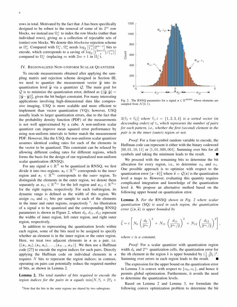
For any signal s ∈ RN to be quantized in RNSQ, we firstdivide it into two regions: s0 ∈ RN0 corresponds to the innerregion and s1 ∈ RN1 corresponds to the outer region. Todistinguish the elements in the outer region, we denote themseparately as s11 ∈ RN11 for the left region and s12 ∈ RN12

for the right region, respectively. For each (sub)region, itsdynamic range is defined as the width of this region. Weassign α0 and α1 bits per sample to each of the elementsin the inner and outer regions, respectively 5. An illustrationof a signal s to be quantized and the corresponding RNSQparameters is shown in Figure 2, where d0, d11, d12 representthe widths of inner region, left outer region, and right outerregion, respectively.

In addition to representing the quantization levels withineach region, some of the bits need to be assigned to specifywhether an element is in the inner region or the outer region.Here, we treat two adjacent elements in s as a pair, i.e.(s1, s2), (s3, s4), . . . , (sN−1, sN ). We then use a Huffmancode [27] to encode the region indices for such pairs. Directlyapplying the Huffman code on individual elements in srequires N bits to represent the region indices; in contrast,operating on pairs can potentially reduce the required numberof bits, as shown in Lemma 2.

Lemma 2. The total number of bits required to encode theregion indices for the pairs in s equals min[N, τ1 + 2τ2 +

5Note that the bits in the outer regions are shared by two subregions.

s

-5 0 5

Cou

nt

0

200

400

600

800

1000

1200

N11

, α1

N12

, α1

N0, α

0

d11

d12

d0

Fig. 2. The RNSQ parameters for a signal s ∈ R30000 whose elements aresampled from N (0, 1).

3(τ3 + τ4)] where τi, i = 1, 2, 3, 4 is a sorted vector (indescending order) of τi, which represents the number of pairsfor each pattern, i.e., whether the first (second) element in thepair is in the inner (outer) region or not.

Proof: For a four-symbol random variable to encode, theHuffman code can represent it either with the binary codeword[00, 01, 10, 11] or [1, 01, 000, 001]. Summing over bits for allsymbols and taking the minimum leads to the result.

We proceed with the remaining bits to determine the bitallocation for every region, i.e., to determine α0 and α1.One possible approach is to optimize with respect to thequantization error ‖s−s‖22 where s = Q(s) is the quantizationlevel s maps to. However, evaluating this quantity requirescomplicated integration and knowledge of the quantizationlevel s. We propose an alternative method based on thefollowing upper bound on quantization error.

Lemma 3. For the RNSQ shown in Fig. 2 where scalarquantization (SQ) is used in each region, the quantizationerror ξ(s, s) is upper bounded by

ξ = c

[N0

(d0

2α0

)2

+ N11

(d11

2α1/2

)2

+ N12

(d12

2α1/2

)2],

where c is a constant.

Proof: For a scalar quantizer with quantization regionwidth dk and 2αk quantization cells, the quantization error forthe ith element in the region k is upper bounded by ( 1

2dk

2αk )2.Summing over errors in each region leads to the result.

The expression for the upper bound on the quantization errorin Lemma 3 is convex with respect to α0, α1, and hence itpermits global optimization. Furthermore, it avoids the needto determine the quantization levels.

Based on Lemma 2 and Lemma 3, we formulate thefollowing convex optimization problem to determine the bit

7

budget assignment:

minimizeα0,α1

N0

(d0

2α0

)2

+N11

(d11

2α1/2

)2

+N12

(d12

2α1/2

)2

subject to N0α0 +N11α1 +N12α1 = Nα− ηα0 ≥ 0, α1 ≥ 0.

(11)where η is the number of bits used to denote the region indicesfrom the Huffman code. When the parameters in RNSQsatisfy

log2 d0 ≤ 1+1

2log2

(N11d

211 +N12d

212

N11 +N12

)+Nα− ηN0

(12a)

and

log2 d0 ≥ 1+1

2log2

(N11d

211 +N12d

212

N11 +N12

)− Nα− ηN −N0

(12b)

the optimal solution to (11) is

α?0 =N −N0

N

[Nα− ηN −N0

+ log2 d0 − 1

− 1

2log2

(N11d

211 +N12d

212

N11 +N12

)]α?1 =

N0

N

[Nα− ηN0

+ 1− log2 d0

+1

2log2

(N11d

211 +N12d

212

N11 +N12

)].

We refer the reader to [28] for background on convex opti-mization, and provide the derivation in Appendix C.

Note that our derivation for the bit budget allocation sofar assumes that the inner and outer quantization regions aregiven, and it remains to give a strategy for determining theseregions. One approach is to fix the bit budgets α0, α1 andthen update the region widths d0, d11, d12. This approach,however, leads to a violation of the bit budget constraintin (11). Instead, we take a grid search approach, by solving(11) over a group of candidate regions and selecting theone which gives the smallest quantization error. We need toguarantee that (12) is satisfied for these candidate regions.Since we have a closed-form solution to (11), this grid searchapproach is efficient to implement. It can also be executed inparallel for different candidate regions, as their correspondingoptimization problems in (11) are independent of each other.

After specifying the bit allocation for each region, weneed to quantize elements within each region. We employLloyd’s algorithm [18] for this task. In contrast to USQ,Lloyd’s algorithm achieves a better match to the measurementdistribution and hence obtains smaller quantization errors. Werefer the reader to [12] for more details on Lloyd’s algorithm.

Lloyd’s algorithm has been shown in Dai et al. [3] tooutperform USQ in terms of reconstruction performance,which is also observed in our experiments in Section V.

V. EXPERIMENTAL RESULTS

We test our proposed sensing matrices and quantizer, byreconstructing sparse signals from quantized compressive sam-ples. For scalar quantization, we implement USQ and the

Lloyd’s algorithm. For vector quantization, we implement thescalar vector quantization (SVQ) [29]. Our evaluation metricfor the quantizers is the relative quantization error, which isdefined as

relative quantization error :=‖y − y‖2‖y‖2

.

To recover the sparse signal, we follow Kostina et al. [7] inusing the SPGL1 toolbox [30] across all of our followingexperiments. All code is written in MATLAB and tested on aLinux machine with 3.1GHz CPU.

A. Simulated Example

We start by simulating a signal x ∈ R1024 with sparsityK = 40, whose non-zero positions are randomly chosenand whose non-zero elements are sampled from N (0, 1). Weset m = 4 and hence all matrices have size 512 × 1024.Following the rejection-based quantization scheme outlined inSection II-A, we obtain the estimated signal x. Our perfor-mance metric is the signal-to-noise ratio (SNR), defined as

SNR := 20 log10

‖x‖2‖x− x‖2

.

To account for the randomness, we repeat the above process100 times and report the average results.

Rejection rate0 0.1 0.2 0.3 0.4 0.5

SN

R (

dB

)

6

8

10

12

14

16

18Stacked Kerdock

Permuted Hadamard

Kostina et al.

Fig. 3. The SNR as a function of the rejection rate for different sensingmatrices, with SVQ as the quantizer and a bit budget of 2 bits/sample. Itwas shown in [7] that Kostina et al. outperforms Laska et al. [5] in a similarsetting.

Figure 3 shows the SNR as a function of rejection ratefor different sensing matrices. When no measurements arerejected, we can conclude that both of our constructionsachieve better reconstruction performance than the construc-tion in Kostina et al. [7], since the same quantizer and recoverysolver have been employed. Both of our constructed matricesshow a general trend of an improvement in SNR with rejec-tion rate, which shows a favourable robustness to rejection,explained by the matrices’ desirable coherence properties (seeSection III).

To compare the performances of different quantizers, werecover the sparse signal using the same stacked Kerdockmatrix. The results are summarized in Figure 4: SVQ achievesthe highest SNR for most of the points; however, it also

8

Rejection rate0 0.1 0.2 0.3 0.4 0.5

SN

R (

dB

)

8

9

10

11

12

13

14

15

16

17

SVQLloydRNSQUSQ

(a)

Rejection rate0 0.1 0.2 0.3 0.4 0.5

CP

U t

ime

(se

co

nd

s)

10 -4

10 -3

10 -2

10 -1

10 0

10 1

SVQRNSQLloydUSQ

(b)

Rejection rate0 0.1 0.2 0.3 0.4 0.5

Rela

tive q

uantization e

rror

0.05

0.1

0.15

0.2

0.25

0.3

0.35

0.4

USQRNSQLloydSVQ

(c)

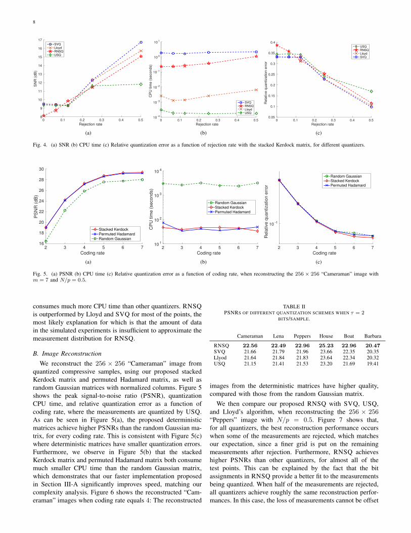
Fig. 4. (a) SNR (b) CPU time (c) Relative quantization error as a function of rejection rate with the stacked Kerdock matrix, for different quantizers.

Coding rate2 3 4 5 6 7

PS

NR

(d

B)

16

18

20

22

24

26

28

30

Stacked KerdockPermuted HadamardRandom Gaussian

(a)

Coding rate2 3 4 5 6 7

CP

U tim

e (

seconds)

101

102

103

104

Random GaussianStacked KerdockPermuted Hadamard

(b)

Coding rate2 3 4 5 6 7

Rela

tive q

uantization e

rror

10-1

Random Gaussian

Stacked KerdockPermuted Hadamard

(c)

Fig. 5. (a) PSNR (b) CPU time (c) Relative quantization error as a function of coding rate, when reconstructing the 256 × 256 “Cameraman” image withm = 7 and N/p = 0.5.

consumes much more CPU time than other quantizers. RNSQis outperformed by Lloyd and SVQ for most of the points, themost likely explanation for which is that the amount of datain the simulated experiments is insufficient to approximate themeasurement distribution for RNSQ.

B. Image ReconstructionWe reconstruct the 256 × 256 “Cameraman” image from

quantized compressive samples, using our proposed stackedKerdock matrix and permuted Hadamard matrix, as well asrandom Gaussian matrices with normalized columns. Figure 5shows the peak signal-to-noise ratio (PSNR), quantizationCPU time, and relative quantization error as a function ofcoding rate, where the measurements are quantized by USQ.As can be seen in Figure 5(a), the proposed deterministicmatrices achieve higher PSNRs than the random Gaussian ma-trix, for every coding rate. This is consistent with Figure 5(c)where deterministic matrices have smaller quantization errors.Furthermore, we observe in Figure 5(b) that the stackedKerdock matrix and permuted Hadamard matrix both consumemuch smaller CPU time than the random Gaussian matrix,which demonstrates that our faster implementation proposedin Section III-A significantly improves speed, matching ourcomplexity analysis. Figure 6 shows the reconstructed “Cam-eraman” images when coding rate equals 4: The reconstructed

TABLE IIPSNRS OF DIFFERENT QUANTIZATION SCHEMES WHEN τ = 2

BITS/SAMPLE.

Cameraman Lena Peppers House Boat Barbara

RNSQ 22.56 22.49 22.96 25.23 22.96 20.47SVQ 21.66 21.79 21.96 23.66 22.35 20.35Llyod 21.64 21.84 21.83 23.64 22.34 20.32USQ 21.15 21.41 21.53 23.20 21.69 19.41

images from the deterministic matrices have higher quality,compared with those from the random Gaussian matrix.

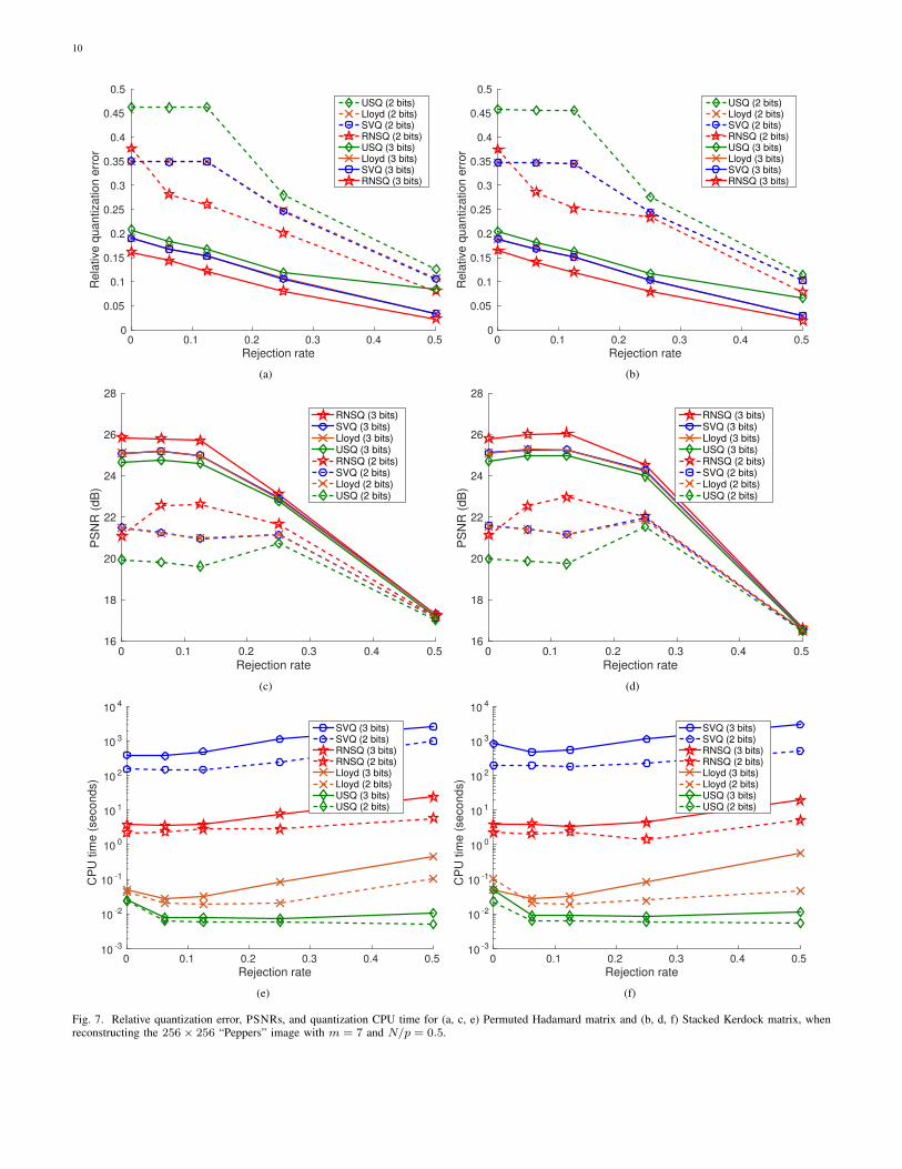
We then compare our proposed RNSQ with SVQ, USQ,and Lloyd’s algorithm, when reconstructing the 256 × 256“Peppers” image with N/p = 0.5. Figure 7 shows that,for all quantizers, the best reconstruction performance occurswhen some of the measurements are rejected, which matchesour expectation, since a finer grid is put on the remainingmeasurements after rejection. Furthermore, RNSQ achieveshigher PSNRs than other quantizers, for almost all of thetest points. This can be explained by the fact that the bitassignments in RNSQ provide a better fit to the measurementsbeing quantized. When half of the measurements are rejected,all quantizers achieve roughly the same reconstruction perfor-mances. In this case, the loss of measurements cannot be offset

9

(a) (b) (c) (d)

Fig. 6. (a) The original “Cameraman” image; the reconstructed “Cameraman” images from (b) stacked Kerdock (c) permuted Hadamard (d) random Gaussianmatrices, when coding rate equals 4 and N/p = 0.5.

by the improvement of quantization, even after we increase thebit budget. Furthermore, we observe that RNSQ consumes lessCPU time than SVQ, which implies that RNSQ has smallercomputational complexity.

To test the robustness of RNSQ, we further compare it withother quantization schemes on other 256×256 images. Table IIshows the best PSNRs achieved from different rejection rates,using the stacked Kerdock matrix. Among all methods, RNSQhas the best reconstruction performance for every image.

VI. CONCLUSION

Finding computational efficient, and hence scalable,schemes for compressive signal reconstruction from quantizedmeasurements is a task of vital practical relevance, for examplein image reconstruction. We have proposed an integratedapproach which addresses both the choice of sampling schemeand the method of quantization itself. We have designed fastsampling transforms specially adapted to addressing saturationerror through measurement rejection, and we have proposeda regionalized non-uniform scalar quantizer which achievesimproved quantization error compared to uniform scalarquantization, while achieving reduced complexity comparedto vector quantization. Our experimental results on imagesdemonstrate empirically that our new scheme is scalable andoutperforms all state-of-the-art methods.

There remain a number of possible avenues for future work,and we wish to mention two in particular. Firstly, it would beexpected that extending RNSQ by performing vector quan-tization within each region would further boost quantizationperformance. Secondly, an important recent body of researchconsiders multi-level sampling schemes for image reconstruc-tion with wavelets [19, 20, 21]. Such sampling schemes areinherently non-democratic, and it is a natural question to askhow the quantization schemes we have proposed in this papercould be combined with multi-level sampling strategies.

APPENDIX APROOF OF ORTHOGONALITY OF M

Using the definition of M in (6),∑(a,b)

M(u1,v1),(a,b)M(u2,v2),(a,b)

=∑(a,b)

(−1)(u1+u2)T a+(v1+v2)T b+ 12 vT1 Rav1+ 1

2 vT2 Rav2

=

2m+1

∑a

(−1)(u1+u2)T a+ 12 vT1 Rav1

×(−1)12 vT2 Rav2 v1 = v2

0 otherwise

=

2m+1∑a

(−1)(u1+u2)T a+vTRav v1 = v2 = v

0 otherwise

=

2m+1∑a

(−1)(u1+u2)T a v1 = v2

0 otherwise,(13)

where in the last step we use the fact that vTRav ≡ 0 (mod 2)for any binary symmetric matrix Ra. This argument appliesequally to the definitions of Ra in both Constructions 1 and2. It then follows from (13) that∑(a,b)

M(u1,v1),(a,b)M(u2,v2),(a,b) =

22m+1 u1 = u2, v1 = v2

0 otherwise,

and so M has orthogonal columns. Since M is also square,it is therefore an orthogonal matrix under appropriate normal-ization.

APPENDIX BPROOF OF CORRECTNESS OF ALGORITHM 1

Consider applying Algorithm 1 to x(a,b) where a ∈ Fm2 , b ∈Fm+1

2 , obtaining the output y(u,v) where u ∈ Fm2 , v ∈ Fm+12 .

Since wa = H(xa) for all a ∈ Fm2 , we have

(wa)v = 2−(m+1)

2

∑b∈Fm+1

2

(−1)bT v(xa)b,

from which it follows that

(zv)a = 2−(m+1)

2 (−1)12vTRav

∑b∈Fm+1

2

(−1)bT vx(a,b).

10

Rejection rate0 0.1 0.2 0.3 0.4 0.5

Re

lative

qu

an

tiza

tio

n e

rro

r

0

0.05

0.1

0.15

0.2

0.25

0.3

0.35

0.4

0.45

0.5

USQ (2 bits)Lloyd (2 bits)SVQ (2 bits)RNSQ (2 bits)USQ (3 bits)Lloyd (3 bits)SVQ (3 bits)RNSQ (3 bits)

(a)

Rejection rate0 0.1 0.2 0.3 0.4 0.5

Re

lative

qu

an

tiza

tio

n e

rro

r

0

0.05

0.1

0.15

0.2

0.25

0.3

0.35

0.4

0.45

0.5

USQ (2 bits)Lloyd (2 bits)SVQ (2 bits)RNSQ (2 bits)USQ (3 bits)Lloyd (3 bits)SVQ (3 bits)RNSQ (3 bits)

(b)

Rejection rate0 0.1 0.2 0.3 0.4 0.5

PS

NR

(dB

)

16

18

20

22

24

26

28

RNSQ (3 bits)SVQ (3 bits)Lloyd (3 bits)USQ (3 bits)RNSQ (2 bits)SVQ (2 bits)Lloyd (2 bits)USQ (2 bits)

(c)

Rejection rate0 0.1 0.2 0.3 0.4 0.5

PS

NR

(dB

)

16

18

20

22

24

26

28

RNSQ (3 bits)SVQ (3 bits)Lloyd (3 bits)USQ (3 bits)RNSQ (2 bits)SVQ (2 bits)Lloyd (2 bits)USQ (2 bits)

(d)

Rejection rate0 0.1 0.2 0.3 0.4 0.5

CP

U t

ime

(se

co

nd

s)

10 -3

10 -2

10 -1

10 0

10 1

10 2

10 3

10 4

SVQ (3 bits)SVQ (2 bits)RNSQ (3 bits)RNSQ (2 bits)Lloyd (3 bits)Lloyd (2 bits)USQ (3 bits)USQ (2 bits)

(e)

Rejection rate0 0.1 0.2 0.3 0.4 0.5

CP

U t

ime

(se

co

nd

s)

10 -3

10 -2

10 -1

10 0

10 1

10 2

10 3

10 4

SVQ (3 bits)SVQ (2 bits)RNSQ (3 bits)RNSQ (2 bits)Lloyd (3 bits)Lloyd (2 bits)USQ (3 bits)USQ (2 bits)

(f)

Fig. 7. Relative quantization error, PSNRs, and quantization CPU time for (a, c, e) Permuted Hadamard matrix and (b, d, f) Stacked Kerdock matrix, whenreconstructing the 256× 256 “Peppers” image with m = 7 and N/p = 0.5.

11

Since yv = H(zv) for all v ∈ Fm+12 , we have

y(u,v) = (yv)u

= 2−m2

∑a∈Fm2

(−1)aTu(zv)a

= 2−(2m+1)

2

∑a∈Fm2

(−1)aTu

∑b∈Fm+1

2

(−1)bT vx(a,b)

=∑a∈Fm2

∑b∈Fm+1

2

2−(2m+1)

2 (−1)aTu+bT v+ 1

2 vTRavx(a,b)

=∑a∈Fm2

∑b∈Fm+1

2

M(u,v),(a,b)x(a,b),

where the last line follows from (6).

APPENDIX CDERIVATION OF THE OPTIMAL BIT ASSIGNMENT IN RNSQ

We first write the objective function in (11) as f(α0, α1) =N0 d

20 2−2α0 +4(N11d

211+N12d

212) 2−2α1 . Plugging the equal-

ity constraint α1 = Nα−η−N0α0

N11+N12into this objective function

and setting ∂f∂α0

= 0, we obtain

α?0 =N −N0

N

[Nα− ηN −N0

+ log2 d0 − 1

− 1

2log2

(N11d

211 +N12d

212

N11 +N12

)].

Subsequently, we have

α?1 =N0

N

[Nα− ηN0

+ 1− log2 d0

+1

2log2

(N11d

211 +N12d

212

N11 +N12

)].

To guarantee both α?0 and α?1 are non-negative, we needto have the constraints for the parameters in RNSQ, shownin (12).

REFERENCES

[1] E. J. Candes, J. Romberg, and T. Tao, “Robust un-certainty principles: Exact signal reconstruction fromhighly incomplete frequency information,” IEEE Trans.Inf. Theory, vol. 52, no. 2, pp. 489–509, 2006.

[2] D. L. Donoho, “Compressed sensing,” IEEE Trans. Inf.Theory, vol. 52, no. 4, pp. 1289–1306, 2006.

[3] W. Dai, H. V. Pham, and O. Milenkovic, “Distortion-rate functions for quantized compressive sensing,” inIEEE Information Theory Workshop on Networking andInformation Theory, vol. 61, 2009.

[4] A. Zymnis, S. Boyd, and E. J. Candes, “Compressedsensing with quantized measurements,” IEEE Signal Pro-cess. Lett., vol. 17, no. 2, pp. 149–152, 2010.

[5] J. N. Laska, P. T. Boufounos, M. A. Davenport, andR. G. Baraniuk, “Democracy in action: Quantization,saturation, and compressive sensing,” Applied and Com-putational Harmonic Analysis, vol. 31, no. 3, pp. 429–443, 2011.

[6] L. Jacques, D. K. Hammond, and J. M. Fadili, “Dequan-tizing compressed sensing: When oversampling and non-gaussian constraints combine,” IEEE Trans. Inf. Theory,vol. 57, no. 1, pp. 559–571, 2011.

[7] V. Kostina, M. F. Duarte, S. Jafarpour, and A. R.Calderbank, “The value of redundant measurement incompressed sensing,” in Proc. IEEE Int. Conf. Acoust.,Speech, Signal Processing, 2011, pp. 3656–3659.

[8] J. Sun and V. Goyal, “Quantization for compressed sens-ing reconstruction,” in SAMPTA’09, 2009, pp. Special–session.

[9] K. Qiu and A. Dogandzic, “Sparse signal reconstruc-tion from quantized noisy measurements via GEM hardthresholding,” IEEE Trans. Signal Process., vol. 60,no. 5, pp. 2628–2634, 2012.

[10] U. S. Kamilov, V. K. Goyal, and S. Rangan, “Message-passing de-quantization with applications to compressedsensing,” IEEE Trans. Signal Process., vol. 60, no. 12,pp. 6270–6281, 2012.

[11] C. Thrampoulidis, E. Abbasi, and B. Hassibi, “The lassowith non-linear measurements is equivalent to one withlinear measurements,” in Annual Conference on NeuralInformation Processing Systems, 2015.

[12] A. Gersho and R. M. Gray, Vector quantization andsignal compression. Springer Science & BusinessMedia, 2012, vol. 159.

[13] A. R. Calderbank and I. Daubechies, “The pros and consof democracy,” IEEE Trans. Inf. Theory, vol. 48, no. 6,pp. 1721–1725, 2002.

[14] A. Shirazinia, S. Chatterjee, and M. Skoglund, “Jointsource-channel vector quantization for compressed sens-ing,” IEEE Trans. Signal Process., vol. 62, no. 14, pp.3667–3681, 2014.

[15] E. J. Candes and T. Tao, “Decoding by linear program-ming,” IEEE Trans. Inf. Theory, vol. 51, no. 12, pp.4203–4215, 2006.

[16] D. L. Donoho and M. Elad, “Optimally sparse repre-sentation in general (nonorthogonal) dictionaries via `1minimization,” Proceedings of the National Academy ofScience, vol. 100, no. 5, 2003.

[17] R. Gribonval and M. Nielson, “Sparse representations inunions of bases,” IEEE Trans. Inf. Theory, vol. 49, no. 12,2003.

[18] S. P. Lloyd, “Least squares quantization in PCM,” IEEETrans. Inf. Theory, vol. 28, no. 2, pp. 129–137, 1982.

[19] J. Romberg, “Imaging via compressive sampling,” IEEESignal Process. Mag., vol. 25, no. 2, pp. 14–20, 2008.

[20] B. Adcock, A. C. Hansen, C. Poon, and B. Roman,“Breaking the coherence barrier: A new theory for com-pressed sensing,” arXiv preprint arXiv:1302.0561, 2013.

[21] F. Krahmer and R. Ward, “Stable and robust samplingstrategies for compressive imaging,” IEEE Trans. ImageProcess., vol. 23, no. 2, pp. 612–622, 2014.

[22] S. S. Chen, D. L. Donoho, and M. A. Saunders, “Atomicdecomposition by basis pursuit,” SIAM review, vol. 43,no. 1, pp. 129–159, 2001.

[23] A. R. Calderbank, S. Howard, and S. Jafarpour, “Con-struction of a large class of deterministic sensing matrices

12

that satisfy a statistical isometry property,” IEEE J. Sel.Topics Signal Process., vol. 4, no. 2, pp. 358–374, 2010.

[24] M. F. Duarte, S. Jafarpour, and A. R. Calderbank, “Per-formance of the Delsarte-Goethals frame on clusteredsparse vectors,” IEEE Trans. Signal Process., vol. 61,no. 8, pp. 1998–2008, 2013.

[25] H. Monajemi, S. Jafarpour, M. Gavish, and D. L.Donoho, “Deterministic matrices matching the com-pressed sensing phase transitions of Gaussian randommatrices,” Proceedings of the National Academy of Sci-ences, vol. 110, no. 4, 2013.

[26] W. Pratt, J. Kane, and H. Andrew, “Hadamard transformimage coding,” Proceedings of the IEEE, vol. 57, no. 1,1969.

[27] T. M. Cover and J. A. Thomas, Elements of InformationTheory, 2nd ed. Hoboken, NJ: Wiley, 2006.

[28] S. Boyd and L. Vandenberghe, Convex Optimization.Cambridge University Press, 2004.

[29] R. Laroia and N. Farvardin, “A structured fixed-ratevector quantizer derived from a variable-length scalarquantizer. I. memoryless sources,” IEEE Trans. Inf. The-ory, vol. 39, no. 3, pp. 851–867, 1993.

[30] E. van den Berg and M. P. Friedlander, “Probing thepareto frontier for basis pursuit solutions,” SIAM Journalon Scientific Computing, vol. 31, no. 2, pp. 890–912,2008.