An instrumental electrode model for solving electrical impedance tomography forward problems

Article (Published Version)

http://sro.sussex.ac.uk

Zhang, Weida and Li, David (2014) An instrumental electrode model for solving electrical impedance tomography forward problems. Physiological Measurement, 35 (10). pp. 2001-2026. ISSN 0967-3334

This version is available from Sussex Research Online: http://sro.sussex.ac.uk/48938/

This document is made available in accordance with publisher policies and may differ from the published version or from the version of record. If you wish to cite this item you are advised to consult the publisher’s version. Please see the URL above for details on accessing the published version.

Copyright and reuse: Sussex Research Online is a digital repository of the research output of the University.

Copyright and all moral rights to the version of the paper presented here belong to the individual author(s) and/or other copyright owners. To the extent reasonable and practicable, the material made available in SRO has been checked for eligibility before being made available.

Copies of full text items generally can be reproduced, displayed or performed and given to third parties in any format or medium for personal research or study, educational, or not-for-profit purposes without prior permission or charge, provided that the authors, title and full bibliographic details are credited, a hyperlink and/or URL is given for the original metadata page and the content is not changed in any way.

This content has been downloaded from IOPscience. Please scroll down to see the full text.

Download details:

IP Address: 139.184.30.133

This content was downloaded on 22/09/2014 at 08:40

Please note that terms and conditions apply.

An instrumental electrode model for solving EIT forward problems

View the table of contents for this issue, or go to the journal homepage for more

2014 Physiol. Meas. 35 2001

2001

Physiological Measurement

An instrumental electrode model for

solving EIT forward problems

Weida Zhang1,2 and David Li1,3

1 Department of Engineering and Design, School of Engineering and Informatics,

University of Sussex, BN1 9SB, UK2 Department of Electronic Engineering, School of Information and Electronics,

Beijing Institute of Technology, 100081, People’s Republic of China3 Strathclyde Institute of Pharmacy and Biomedical Sciences, University of

Strathclyde, G4 0RE, Scotland, UK

E-mail: wz39@sussex.ac.uk and david.li@strath.ac.uk

Received 28 February 2014, revised 22 May 2014

Accepted for publication 9 June 2014

Published 19 September 2014

Abstract

An instrumental electrode model (IEM) capable of describing the performance of

electrical impedance tomography (EIT) systems in the MHz frequency range has

been proposed. Compared with the commonly used Complete Electrode Model

(CEM), which assumes ideal front-end interfaces, the proposed model considers the

effects of non-ideal components in the front-end circuits. This introduces an extra

boundary condition in the forward model and offers a more accurate modelling

for EIT systems. We have demonstrated its performance using simple geometry

structures and compared the results with the CEM and full Maxwell methods. The

IEM can provide a signiicantly more accurate approximation than the CEM in

the MHz frequency range, where the full Maxwell methods are favoured over the

quasi-static approximation. The improved electrode model will facilitate the future

characterization and front-end design of real-world EIT systems.

Keywords: electrical impedance tomography (EIT), complete electrode

model, instrumental EIT, inite elements, EIDORS, non-ideal front-ends

(Some igures may appear in colour only in the online journal)

1. Introduction

Electrical impedance tomography (EIT) (Barber and Brown 1984, Cheney et al 1999, Holder

2005, Metherall et al 1996, Saulnier et al 2001, Webster 1990), is a technique for determining

Institute of Physics and Engineering in Medicine

Content from this work may be used under the terms of the Creative Commons Attribution 3.0

licence. Any further distribution of this work must maintain attribution to the author(s) and the title

of the work, journal citation and DOI.

0967-3334/14/102001+26$33.00 © 2014 Institute of Physics and Engineering in Medicine Printed in the UK

Physiol. Meas. 35 (2014) 2001–2026 doi:10.1088/0967-3334/35/10/2001

W Zhang and D Li

2002

Physiol. Meas. 35 (2014) 2001

the distribution of the conductivity or admittivity in a volume by injecting electrical currents

into the volume and measuring the corresponding potentials on the surface of the volume.

A 3D image of the conductivity distribution is generated by using inverse algorithms, which

includes a so-called forward problem capable of predicting the voltages on deined surface

electrodes for a given conductivity distribution (Lionheart 2004).

EIT has been applied to cancer diagnosis applications. It is desirable to operate in the 0.1–

10 MHz band since a difference in admittivity between malignant and normal tissues can be

observed in this frequency range (Grimnes and Martinsen 2008, Schwan 1957, Surowiec et al

1988). Recently, several image reconstruction methods have been proposed to enhance the EIT

contrast, but only in the frequency range of tens of kHz (Ahn et al 2010, Harrach et al 2010, Jun

et al 2009, Seo et al 2008). There are two major problems in extending the operating frequency

of EIT systems. Firstly, it is dificult to obtain accurate measurements from experimental devices

when the operating frequency increases. The instrumental effects including non-idealities of the

sources, measurement devices and parasitic capacitance (from the cables, connectors or the elec-

trodes themselves), etc., start to degrade the measurement accuracy at frequencies larger than

hundreds of kHz. Secondly, the Laplace equation used by the EIT forward problem is an approxi-

mation derived from Maxwell’s equations (Boyse et al 1992, Boyse and Paulsen 1997, Paulsen

et al 1992, Soni et al 2006). The ‘irrotational electric ield’ approximation tends to fail when the

frequency increases, as the quasi-static assumption is no longer valid (Sheng and Song 2012).

For the irst problem, we found that the boundary conditions (BCs) used for forward prob-

lems are not suficient for system modelling in the low MHz band. There are different kinds

of BCs used in the EIT forward problems, including the Gap Model (Boyle and Adler 2010),

Shunt Electrode Model (Boyle and Adler 2010) and Complete Electrode Model (CEM) (Boyle

and Adler 2010, Cheng et al 1989, Somersalo et al 1992, Vauhkonen et al 1999). The CEM

constrains the electrical currents lowing on the electrode surfaces and on the boundary of the

imaging volume. It also includes the contact impedance on the electrode surface and therefore

accounts for the voltage difference between the electrode and the outer surface of the imaging

volume. It has been reported that the CEM can match experimental results with a very high

precision up to 0.1 % (Somersalo et al 1992). To reconstruct accurate images from in vivo

data an accurate electrode model is usually required, and thus, the CEM is generally preferred

(Boyle and Adler 2010). The accuracy of CEM solutions depends on accurate measurements or

estimations of the contact impedance. Methods and results have been reported to estimate the

contact impedance for CEM (Boverman et al 2007, Demidenko 2011, Demidenko et al 2011).

The CEM, however, assumes that the system hardware is ideal and therefore does not

consider the loading effects of the current excitation sources or the voltage measurement

components. This assumption is only valid at frequencies much lower than 1 MHz. Several

research groups have described design implementations, simulations and experiment results

using hardware with current source output impedances measured in MΩ at frequencies up to

hundreds of kHz (Denyer et al 1994). Usually the input impedance of the front-end ampliiers

in voltage measurement components (such as op-amp follower (Oh et al 2011) or instrumen-

tation ampliier (Oh et al 2007a)) is around several GΩ.

To overcome the irst problem, the requirements for high output/input impedance of the

excitation/measurement circuits pose a signiicant challenge in hardware implementation, espe-

cially at high frequencies, and therefore impose a limitation on the effective use of the forward

model. Recent research efforts have been devoted to enhancing the output impedance of current

sources, such as using driven shields and generalized impedance converters (GIC) (Ross et al

2003). It has been shown that a GIC can increase the output impedance up to 2 MΩ at 495 kHz

(Oh et al 2011). Another method for modelling and optimising the hardware of EIT systems

has been proposed (Hartinger et al 2006) using a Howland current source and a bootstrapped

W Zhang and D Li

2003

Physiol. Meas. 35 (2014) 2001

follower to model the hardware effects and optimise the parameters of the circuit, but it only

improved the performance at frequencies less than 100 kHz. An image reconstruction method

has been reported in which hardware effects were modelled through modiication of the system

matrix used for the inversion (Hartinger et al 2007). However, the reported operating frequency

was much lower than 500 kHz as there was no optimisation of the forward model.

For the quasi-static approximation, which is the second problem mentioned earlier, a inite

element analysis method derived from the full Maxwell equations (called the A − Φ formulation)

has been proposed (Soni et al 2006) and the formulations (which did not apply the quasi-static

assumption) have been applied to voltage source based systems operating up to 10 MHz (Halter

et al 2004, Halter et al 2008). Being derived from the full Maxwell equations, the formulation

is very computationally intensive compared to a Laplace formulation. A calibration method is

used for compensating the instrumental effects (which also appear in voltage source systems).

Several calibration algorithms have been proposed for correcting the measurement errors

caused by hardware non-idealities (Halter et al 2008, Holder 2005, McEwan et al 2006, Oh

et al 2007a). These effectively compensate the instrumental effect on driving electrodes but

it is dificult to remove all instrumental effects (including measuring electrode error) in the

frequency range we are considering.

The proposed instrumental electrode model (IEM) considers the effects on the potential

distribution in the volume caused by hardware non-idealities, especially at frequencies larger

than 500 kHz. An extra boundary condition is introduced accordingly to the CEM in the for-

ward problem. The IEM can provide a much more accurate representation of the overall sys-

tem including instrumental effects introduced by the hardware (the irst problem mentioned).

It is worth noting that although the two previously mentioned effects are normally combined

when operating in the MHz frequency range, they do not always occur together. The instru-

mental effect is due to hardware non-idealities and depends on the parameters of the hardware

alone, while the full Maxwell effect is caused by the quasi-static assumption and depends on

the admittivity and permeability of the material and the overall system geometry and scale size.

In this paper, we will derive the IEM forward model and compare with the results obtained

from the CEM, from A − Φ formulations (derivations for 3D problems are attached in

appendix A based on the equations for 2D problems derived in Soni et al (2006)) and from

COMSOL Multiphysics (commonly used commercial Maxwell solvers) to assess the com-

parative performance over the frequency range of interest.

The paper is organized as follows. Section 2 describes the forward problem formulation as

usually applied in EIT. The IEM is detailed in section 3 based on the CEM. A lumped-circuit

model and a tank model are solved by the above methods in section 4 and their results are

cross-compared and discussed. The conclusions are presented in section 5.

The paper is mainly focused on current source EIT systems. We believe that the instru-

mental non-idealities would bring similar impacts to both current source and voltage source

EIT systems based on circuit theory. Demonstrating such impacts on a current source system

should be able to shed a light on how instrumental non-idealities deteriorate system perfor-

mances. The IEM formula for typical voltage source systems, however, is also derived with an

example included in the appendix B, as voltage source systems are also widely used.

2. Forward problem

The forward problem for the volume under consideration can be formulated from Maxwell’s

equations,

ωμ∇ × = −E Hi , (2.1a)

W Zhang and D Li

2004

Physiol. Meas. 35 (2014) 2001

ωε∇ × = +H J Ei , (2.1b)

where E is the electric ield, H is the magnetic ield, ω is the angular frequency, μ and ε are

the electrical permittivity and magnetic permeability respectively, and J = σE with σ being the

conductivity. With the complex permittivity or so-called admittivity, ε* = σ + iωε, substituted

in the equation (2.1b) we have

σ ωε ε∇ · ∇× = ∇· + = ∇· * =H E E E( ) ( i ) ( ) 0. (2.2)

As electric ields often contain singularities, electric potentials are used instead. In computa-

tional electromagnetics (Sheng and Song 2012), the electric potential Φ is also called the sca-

lar potential in contrast with the vector potential A or magnetic potential which are deined as

ω

= ∇ ×

= −∇ Φ−

B A

E A

,

i . (2.3)

The electric ield E consists of an irrotational part (∇Φ) and a rotational part (iωA). From

equation (2.2) and equation (2.3), we obtain

ε ω= ∇ ∇Φ + A0 · * ( i ) . (2.4)

The vector potential is usually ignored in EIT systems, considering the operating frequency or

the geometric scale of the problem. The Maxwell equation is therefore reduced to a Laplace

equation at low frequencies using the well-known quasi-static approximation,

ε ω ε∇ ∇Φ + ≃ ∇ ∇Φ =A· * ( i ) · * 0. (2.5)

Equation (2.5) is the governing equation for EIT systems. Many experimental results have

been presented (Halter et al 2008, Holder 2005) which demonstrate that the approximation

performs equivalently to the full Maxwell solutions at low frequencies.

3. Boundary conditions and numerical solutions

3.1. IEM boundary conditions

To solve the partial differential equation (2.5), proper boundary conditions should be applied

to describe the current injection and model the behaviour of electrodes. The CEM (Cheng et al

1989, Somersalo et al 1992, Vauhkonen et al 1999) is commonly used and has been experi-

mentally proven to be accurate in low frequency EIT systems. The proposed IEM is based on

the CEM, but instrumental non-ideality is given additional consideration within the electrode

model. These boundary conditions can be understood from igure 1. Here we use a current

source EIT system for this demonstration, and for those who interested in voltage source sys-

tems please see the appendix B.

Referring to the EIT electrode model in igure 1, each electrode can be conigured either as

a driving electrode (with the switch closed and the current source connected to the electrode)

or as a measuring electrode (with the switch opened and the current source disconnected).

The current source has an output impedance ZO with the electrode contributing some parasitic

capacitance CS to ground, and the measurement circuit can be modelled with an input imped-

ance ZI. The current source generates a current of I lS .

In the ideal situation, ZO and ZI are assumed to be ininite, CS to be zero, and all of the

current generated from the source goes into the electrode, I lS = Il, when the switch is closed.

When the switch is opened (the circuit acts as a measurement circuit), Il = 0.

W Zhang and D Li

2005

Physiol. Meas. 35 (2014) 2001

The frequency of interest for many EIT applications extends up to several MHz, and dif-

iculties therefore emerge when applying the CEM. Some of the assumptions in the ideal situ-

ation mentioned above need to be re-examined and modiied, since non-ideal loading effects

are not negligible in the MHz frequency range.

Firstly, the output impedance ZO of the current source and input impedance ZI of the

measurement circuit are not ininitely high. The circuit front-ends can easily contribute a

few pF of parasitic capacitance contributed by the devices, therefore reducing input/output

impedances and degrading the performance in the MHz range. In addition the parasitic

capacitance of the cable, PCB trace and electrode itself (modelled by CS in general) is not

negligible. Although CS almost remains constant across the frequency range, the equivalent

impedance of the capacitance 1/(iωCS) reduces and starts loading the front-ends as the fre-

quency increases.

At high frequencies, the electrode current lows therefore behave differently. In con-

trast to the assumption made by the CEM, at high frequencies some portion of I lS lows

through ZO, ZI and CS (this part is negligible when the frequency is low) rather than

entirely into the electrode. Also, for electrodes in measuring mode (with the switch open),

there is some current lowing through ZI and CS to ground, as Il, even though there is no

driving current I lS .

Analytical calculations based on typical circuit parameters provide some indication of typi-

cal input and output impedances. When the operating frequency is 1 MHz, the output imped-

ance ZO typically comprises a resistance of 5 MΩ in parallel with a capacitance of 4 pF and the

input impedance ZI comprises a resistance of 10 MΩ in parallel with a capacitance 4 pF (This

comes from an easily accessible front-end ampliier, for example, 4.5 pF from the Analog

Devices AD8065 or 6 pF from the Texas Instruments OPA2365.) and a parasitic capacitance

CS of 2 pF. At 1 MHz, the overall instrumental effect is modelled with a virtual impedance

ZF, as shown in igure 1, and becomes 16 kΩ in driving mode and 26 kΩ in measuring mode,

which is far from ininite.

For EIT systems working at lower frequencies (< 500 kHz), the GIC (Oh et al 2011, Oh

et al 2007b, Ross et al 2003) is widely used to alleviate the effects of capacitive loading, but

it performs poorly at frequencies higher than 500 kHz.

From the above calculations, it is obvious that there is a signiicant ‘leakage current’

lowing through the instrumental path (with an equivalent impedance of ZF) from the cur-

rent source (in the driving mode) or from the imaging volume (in the measuring mode) and

for accurate representation this leakage current must be included when solving the system

matrix.

We can reformulate the electrode model to include the ‘leakage currents’ in the forward

problem. We obtain, in the driving mode,

+−

+ =IV V

IZ

0,ll

lSGND

F

and in the measuring mode,

−+ =

V VI

Z0,

ll

GND

F

combined as

+ + =IV

IZ

0.ll

lSF

(3.1)

W Zhang and D Li

2006

Physiol. Meas. 35 (2014) 2001

Together with the CEM BCs, we have the IEM as

ε ∇Φ =n* · 0 (Surface not on electrodes) , (3.2a)

∫ ε ∇Φ = S I ln* · d (Surface on th electrode) ,S

ll

(3.2b)

ηεΦ + ∇Φ = Vn* · ,l (3.2c)

∑

+ + =

==

IV

I

I

Z0,

0.

ll

l

l

L

l

SF

1

(3.2d)

Note that, with the external circuit attached, the total current generated from current sources

∑=

Il

L

l1

S may not be balanced any more (as ZF on different driving electrodes may vary), but

the total charge in the volume to be solved ∑=

Il

L

l1

has to be zero.

Figure 1. EIT electrode geometry and circuit model.

where Ω is the volume to be solve,

∂Ω is the surface of the volume,

E is a designator for the electrode circuit node,

n is the outward normal vector on the volume surface,

Sl is the surface of the lth electrode,

Il is the current of the lth electrode,

η is the contact impedance in Ω · m2,

Vl is the voltage measured on the lth electrode,

I lS is the current output by the source, connected with the lth electrode,

CS is the total parasitic capacitance of the cable, PCB trace and electrode itself,

ZO is the output impedance of the current source,

ZI is the input impedance of the voltage measurement device,

and ZF is the virtual impedance, equivalent to the total effect of the above impedance.

For the remaining symbols in the igure we kept the previous deinitions.

W Zhang and D Li

2007

Physiol. Meas. 35 (2014) 2001

In our IEM formulations, the potential balance condition ∑=

Vl

L

l1

used in CEM is removed.

As the CEM does not have a reference ground, whereas the IEM embeds one in the instru-

mental circuit.

When the operating frequency is low enough, the current lowing through the instrumental

path ZF is negligible, in which case the IEM will behave just like the CEM.

The IEM provides a method for describing non-ideal hardware behaviours and is therefore

able to obtain accurate solutions of the forward problem with knowledge of the hardware,

unlike the CEM which assumes perfect hardware.

3.2. Numerical modelling with IEM

Finite element methods (FEM) are used for solving the forward model with the IEM. Our

programs were developed based on the software package EIDORS (Electrical Impedance

and Diffuse Optical Reconstruction Software). EIDORS is a Matlab toolkit for three-dimen-

sional EIT (Adler and Lionheart 2006, Polydorides and Lionheart 2002, Soleimani et al

2005). To apply our IEM model, similar formulations were derived, but with modiications.

We use equation (2.5) and the IEM derived in section 3 as our formulations. Applying

the vector derivative identity, Green’s identity and divergence theorem, we obtain the

weak form:

∫ ∫ε ε∇ ∇Φ = ∇Φ∂

v V v Sn* · d * · d ,Ω Ω

(3.3)

where v is an arbitrary test function.

With the Non-Electrode surface BC equation (3.2a) included,

∫ ∫∑ε ε∇ ∇Φ = ∇Φ=

v V v Sn* · d * · d .

l

L

SΩ1 l

(3.4)

Two unknowns are added to the system equations; one of them is Vl, the potential on electrode

circuit ‘node E’, and the other is Il, the current through the volume to be solved. Equation (3.2c)

is used to add the extra unknown Vl,

∫ ∫ ∫∑ ∑εη η

∇ ∇Φ + Φ − =

= =

v V v SV

v S* · d1

d d 0.

l

L

Sl

Ll

SΩ1 1l l

(3.5)

To constrain Vl, we substitute equation (3.2c) into equation (3.2b) to derive extra equations for

Vl with the other unknown Il involved, hence,

∫η

− Φ− =

VS Id 0.

S

ll

l

(3.6)

To constrain Il, we have the additional equation (3.1), with the known instrument impedance

as the factor,

+ = −V

I IZ

.l

l lF

S (3.7)

Imposing the constraint of charge balance, equation (3.7) becomes

∑− = −

=

−

VI I

Z.

L

l

L

l LF 1

1

S (3.8)

W Zhang and D Li

2008

Physiol. Meas. 35 (2014) 2001

Finally, we obtain

∫ ∫ ∫

∫

∑ ∑

∑

εη η

η

∇ ∇Φ + Φ − =

− Φ− =

+ = − = ⋯ −

− = −

= =

=

−

v V v SV

v S

VS I

VI I l L

VI I

Z

Z

* · d1

d d 0,

d 0,

, 1, 2, 1,

.

l

L

Sl

Ll

S

S

ll

ll l

L

l

L

l L

Ω1 1

FS

F 1

1

S

l l

l

(3.9)

Using Galerkin’s Method we insert the shape functions, ∑ ϕΦ ==

uj

N

j j1

and v = ϕi in

equation (3.9) and lead to the system matrix in the form

+

− =

−

×

×

×

×

×

⎛

⎝

⎜⎜

⎞

⎠

⎟⎟

⎛

⎝⎜⎜

⎞

⎠⎟⎟

⎛

⎝

⎜⎜⎜

⎞

⎠

⎟⎟⎟

A B C

C D

E F

0

0

uv

i

0

0

iS

,

N L

L L

L N

N

LT

1

1I

∫

∫

∫

∑

ε ϕ ϕ

ηϕ ϕ

ηϕ

η

= ∇ ∇ ∈ ℂ

= ∈ ℂ

= − ∈ ℂ

= ∈ ℂ

= ∈ ℂ

×

=

×

×

×

×

⎧⎨⎩

⎫⎬⎭

⎧⎨⎩

⎫⎬⎭

A

B

C

D

E

V

S

S

S

Z

* · d , ,

1d , ,

1d , ,

diag , ,

diag1

, ,

i jN N

l

L

Si j

N N

Si

N L

l L L

L L

Ω

1

F

l

l

⎡

⎣

⎢⎢⎢⎢

⎤

⎦

⎥⎥⎥⎥

=

⋯

⋮ ⋱ ⋮

− − ⋯ −

∈ℜ ×F

1 0 0 0

0 1 0 0

0 0 1 0

1 1 1 0

, ,L L

where ×L LI is identity matrix, ×uN 1 is the nodal potential vector (made up with uj),

×vL 1 is the

electrode voltage vector(made up with Vl), ×iL 1 is the electrode current vector (made up with Il),

×i LS

1 is the source injection current vector (made up with ISl), ϕi, j is the shape functions, N is

the total number of the vertices, and i j, are the index of vertices.

Compared with the CEM, our IEM adds the matrix ×L LI providing extra freedom to the elec-

trode current, and regulates the electrode current by E and F. When the frequency increases

with the ZF reduced, Ev increases and therefore reduces the current applied on the products

CTu and Dv in the driving mode. For the measuring mode, (although the imposed source cur-

rent ISl is zero) Ev + Fi allows the current to low through electrodes. While on the other hand,

if the frequency is low, ZF tends to ininity and the system matrix is equivalent to the CEM.

W Zhang and D Li

2009

Physiol. Meas. 35 (2014) 2001

In addition, the process to ind the ground node is removed, as the ground node is embedded

in the IEM formulations.

4. Case studies and discussions

The following sections illustrate solutions of the forward model for two different geometry

models and compare the results obtained using different solution methods.

4.1. Lumped model

The irst geometry model, called ‘Lumped Model,’ is a cylinder with two electrodes at each

end. The cylinder is illed with materials to simulate breast tissues (Surowiec et al 1988) and

placed in free space as igure 2 deines.

In contrast to typical EIT models, the Lumped Model is clearly not able to predict the

impedance distribution inside the volume without the prior knowledge of its homogeneity,

as there are not enough electrodes. The free space outside the cylinder is usually ignored.

The beneit of the Lumped Model is that as long as the free space (in the sphere) is removed,

then it can be veriied analytically by considering the model as a lumped circuit containing

a parallel-plate capacitor CS in parallel with a resistor RS. As the material in the cylinder is

homogeneous, the circuit components are given as

σ

ε

ε= = =

+

=*

ω

ωS

S

SZR

L, C

L,

R

R

L,S S S

S1

i C

S1

i C

S

S

where RS, CS and ZS are the equivalent resistor, capacitor and impedance of the material, σ, ε

and ε* are the conductivity, permittivity and admittivity of the material, S is the surface area of

the electrode (also the top/bottom surface area of the cylinder), L is the distance between the

electrodes (also the length of the cylinder).

Figure 2. the geometry of the Lumped Model.

W Zhang and D Li

2010

Physiol. Meas. 35 (2014) 2001

In addition, on each electrode, a circuit unit consisting of a resistor RF and a capacitor CF

can be attached to simulate the instrumental impedance ZF we proposed in the IEM. Because

there are only two electrodes in the model, current sources are applied on both of them in

opposite direction and no measuring electrode is included.

When the surrounding free space is considered, the two electrodes form another capacitor

(relecting the interaction with the free space electric ield) connected in parallel with ZS. We

denote it as CA or its reactance XCA, and solve it numerically.

As mentioned in the Introduction, the Laplace equations under the quasi-static approxi-

mation are not suficient to obtain accurate solutions for the frequency range of interest. Here

we denote the difference between the solutions obtained from the full Maxwell equations and

the Laplace equations as the full Maxwell effect, and we use a circuit unit +ZM to model this

effect although a simplistic equivalent impedance cannot fully represent this effect.

The equivalent circuit of the Lumped Model is shown in igure 3.

In our simulations, three main effects are included in the Lumped Model for solving the forward

models. Note that we are not trying to quantify these effects, as they vary with geometries and

materials, but merely to use the combinational effects to verify the IEM. These three effects are:

•Instrumentaleffect,ZF;

•VolumeCut-offeffect,XCA;

•FullMaxwell’seffect, +ZM .

We obtained the simulation results by using the following nine methods (forward problem

solvers or BCs sets) and cross-compared the results to assess the accuracy of the IEM imple-

mentation. The methods are:

(a) analytical lumped method

An analytical solution based on an equivalent circuit of the cylinder and current sources.

(b) analytical lumped method with the instrumental effect ZF

Similar to (a), but the instrumental impedance effect ZF is also included in the analysis.

(c) CEM by EIDORs (Polydorides and Lionheart 2002) without considering the free

space (no XCA)

Figure 3. The equivalent circuit for Lumped Model. (a) For method (a)–(g). (b) For method (h) and (i).

(a) (b)

W Zhang and D Li

2011

Physiol. Meas. 35 (2014) 2001

An FEM forward model of the cylinder solved with the CEM. This models the potential

distribution in the cylinder, contact impedance and the potentials on the two electrodes.

Only the cylinder (coloured in dark red in igure 2) is meshed and solved without consid-

ering the surrounding free space (or XCA).

(d) CEM by EIDORs with XCA

Similar to (c), but with the free space (in igure 2) included and solved. Note that the

governing equation (2.5) and the derivation in section 3.2 are free of sources inside the

volume, which differs from the coniguration for this simulation (the source electrodes

are inside the inite elements volume). They are equivalent mathematically, but we do not

need to detail the equations here.

(e) IEM without considering the free space (no XCA)

Similar to (c), but using the IEM we proposed in the section 3. It models the potential dis-

tribution in the cylinder, contact impedance on the two electrodes with the instrumental

effect ZF included.

(f) IEM with XCA

Similar to (e), but the free space (XCA) is included in the simulations.

(g) A − Φ forward model in Helmholtz equations

An FEM forward model that solves the full Maxwell equations. It models the vector

potential (A) and scalar potential (Φ) distribution in the cylinder and also the surrounding

free space shown in igure  2, but the contact impedance or instrumental effect is not

considered. We derived the formula of the A − Φ method based on a previously published

2D work (Soni et al 2006), and the data structure in Matlab is based on EIDORS using

the mesh generating software NETGEN. A description of the forward model formulation

can be found in the appendix.

(h) COMSOL Multiphysics without the instrumental effect ZF

The solution is obtained by COMSOL Multiphysics (well-known commercial inite-

element software developed for solving differential equations  in different applications,

denoted as COMSOL hereafter). It models the electric ield distribution in the cylinder

and the surrounding free space (perfect matching layer, PML, is usually used in solving

Maxwell’s equations).

(i) COMSOL Multiphysics with ZF

Similar to (h), but we included the instrumental effect ZF on electrodes.

Table 1 summarises the methods we used.

For all methods the dimensions of the cylinder, conductivity, permittivity, instrumen-

tal impedance, stimulation and frequencies are kept constant to allow fair comparison. The

parameters are:

•Materialconductivity,0.03 S m −  1, (Surowiec et al 1988);

•Materialrelativepermittivity,40,(Surowiecet al 1988);

•Cylinderradius,0.01 m; •Cylinderlength,0.10 m; •Currentsourcedrivingcurrent,1 mA; •Frequencyrange,250 kHz–20 MHz.

Various other parameters apply to some of the individual methods:

•TheequivalentimpedanceofthecylinderZS in (a) and (b) is calculated from the material

property and cylinder dimension above.

•Theresistivepartoftheinstrumentalimpedance,RF, in methods (b), (e) and (f) is 5 MΩ.

•Thecapacitivepartoftheinstrumentalimpedance,CF, in methods (b), (e) and (f) is 10 pF.

W Zhang and D Li

2012

Physiol. Meas. 35 (2014) 2001

•Thediameterofthefreespacesphereinmethods(d),(f)and(g)is0.15 m. •ThediameterofthefreespaceplusPMLsphereinmethod(h)and(i)is0.15 m. •Method (h) and (i) which uses COMSOL requires a uniform ‘port’ deined as ield

excitation, so the two opposing electrodes are considered as a single ‘port’, and the

instrumental impedance, which is attached on each electrode in methods (b), (e) and (f), is

combined into a single effective impedance connected in parallel with the port, as shown

in igure 3(b) (with the impedance doubled to maintain equivalence with igure 3(a)).

igures 4 and 5 show the differential voltage in magnitude and phase obtained by the

methods, (a)–(i).

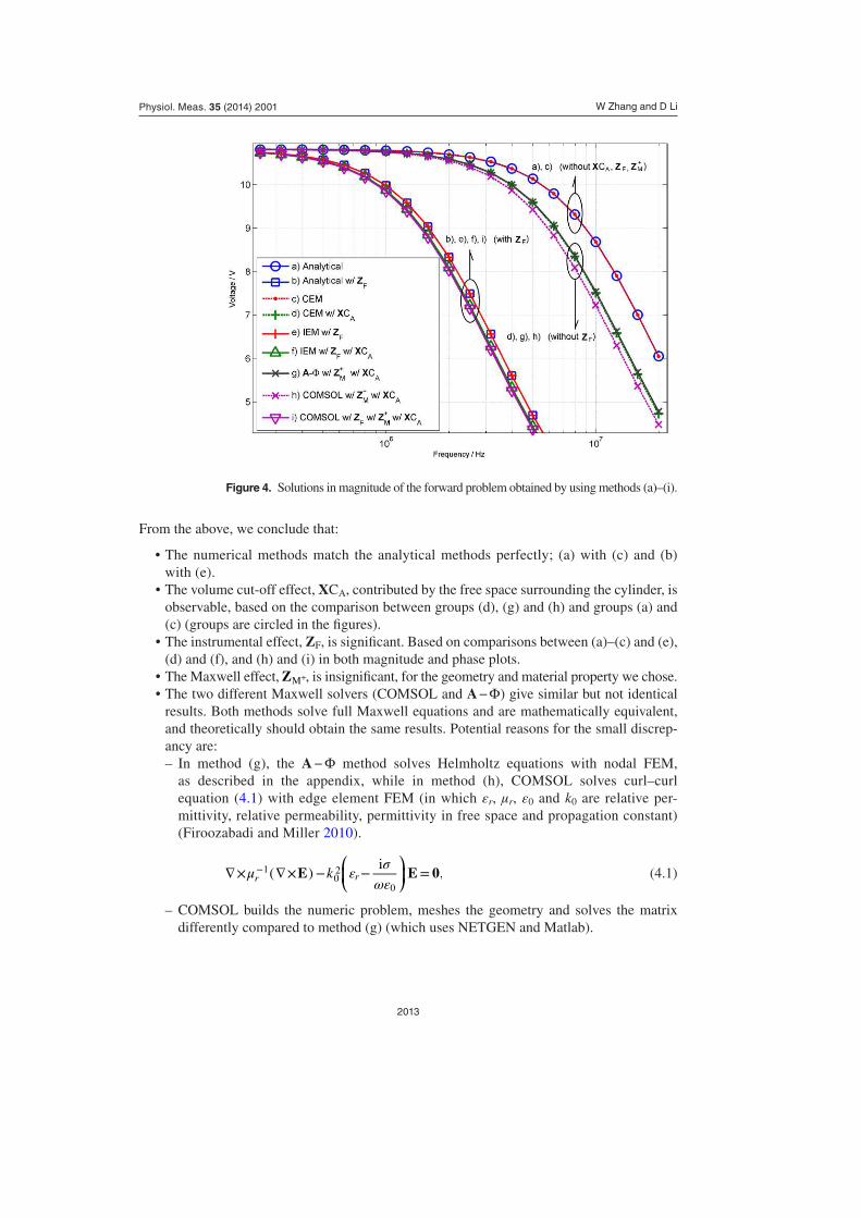
Key indings from the various solution methods are as follows:

•The results from (a), analyticalmethod, and (c),FEMwithCEMBCsare almost thesame, as they describe the same problem in analytical and numerical ways.

•Theresultsfrom(b),analyticalmethodwithZF, and (e), FEM with IEM BCs are in a

good agreement, as they describe the same problem. And this shows our IEM describes

the instrumental effect correctly.

•Both(b)and(e)starttoattenuateatamuchlowerfrequencythan(a)and(c).Thiscomesfrom the instrumental effect, where ZF provides an extra path for the current and reduces

the current injected into the cylinder.

•Similarly,theresultsfor(d),FEMwithCEMBCsandXCA, attenuate in magnitude at

a lower frequency than the (a) and (c) results. This illustrates the volume cut-off effect.

The capacitance contributed by the free space is not considered in (a) and is numerically

chopped off in (c), which provides an extra path for the current.

•Similarly,theresultsfor(f),FEMwithIEMBCsandXCA, also shows the volume cut-off

effect, but are not so different from the results for (b) and (e). This demonstrates that the

instrument effect dominates in this case.

•Theresultsfor(g),FEMofA − Φ problem with XCA, are very similar to the results for

(d), FEM with CEM BCs and XCA. This shows that the full Maxwell effect +ZM is not

obvious for the structure we chose in this frequency range.

•The(h)curves(obtainedusingCOMSOL,butwithoutconsideringZF) are similar to the

(d) curves, showing further that the Maxwell effect is not signiicant. The error between

(g) and (h) will be discussed shortly.

•Theresultsfor(i)usingCOMSOL(includingZF) show the combined effects of ZF, XCA

and +ZM , and they are close to the results for (f).

Table 1. List of the effects considered by each method.

Index Name Effect ZF Effect XCA Effect +ZM

(a) Analytical No No No(b) Analytical w/ZF Yes No No(c) CEM No No No(d) CEM w/XCA No Yes No(e) IEM Yes No No(f) IEM w/XCA Yes Yes No(g) A − Φ No Yes Yes(h) COMSOL No Yes Yes(i) COMSOL w/ZF Yes Yes Yes

Note: The contact impedance in (c)–(f) is set to be 1 × 10  −  6Ω · m2 in order to compare with other

methods which the contact impedance are not considered.

W Zhang and D Li

2013

Physiol. Meas. 35 (2014) 2001

From the above, we conclude that:

•Thenumericalmethodsmatch theanalyticalmethodsperfectly; (a)with (c) and (b)with (e).

•Thevolumecut-offeffect,XCA, contributed by the free space surrounding the cylinder, is

observable, based on the comparison between groups (d), (g) and (h) and groups (a) and

(c) (groups are circled in the igures).

•Theinstrumentaleffect,ZF, is signiicant. Based on comparisons between (a)–(c) and (e),

(d) and (f), and (h) and (i) in both magnitude and phase plots.

•TheMaxwelleffect, +ZM , is insigniicant, for the geometry and material property we chose.

•ThetwodifferentMaxwellsolvers(COMSOLandA − Φ) give similar but not identical

results. Both methods solve full Maxwell equations and are mathematically equivalent,

and theoretically should obtain the same results. Potential reasons for the small discrep-

ancy are:

– In method (g), the A − Φ method solves Helmholtz equations  with nodal FEM,

as described in the appendix, while in method (h), COMSOL solves curl–curl

equation (4.1) with edge element FEM (in which εr, μr, ε0 and k0 are relative per-

mittivity, relative permeability, permittivity in free space and propagation constant)

(Firoozabadi and Miller 2010).

⎛

⎝⎜

⎞

⎠⎟μ ε

σ

ωε∇× ∇× − − =

− kE E 0( )i

,r r1

02

0

(4.1)

– COMSOL builds the numeric problem, meshes the geometry and solves the matrix

differently compared to method (g) (which uses NETGEN and Matlab).

Figure 4. Solutions in magnitude of the forward problem obtained by using methods (a)–(i).

W Zhang and D Li

2014

Physiol. Meas. 35 (2014) 2001

4.2. Tank model and discussion

For the second forward problem we use a simple cylinder tank as shown in igure 6 (relatively

simple to model but complicated enough to illustrate the differences between the IEM and

the other methods). There are six electrodes located at the vertical mid-point of the cylinder

wall with free space surrounding the tank. Each electrode is modelled as a small circle dis-

tributed around the perimeter of the cylinder tank at a uniform 60-degree angular spacing.

Furthermore, a more realistic contact impedance is introduced in this forward problem.

The electrochemical (polarization) impedance part of the contact impedance (Kolehmainen

et al 1997) is considered. Based on experimental measurements of polarization impedance

(Mirtaheri et al 2005), we set the contact impedance of electrodes in the Tank Model using

0.9 % -saline-gold data measured at 1 kHz. It is the highest frequency measured in the report

and the experimental results suggest that the impedance tends to reduce with increasing

frequency (Mirtaheri et al 2005), so we can expect the effect of contact impedance is less

signiicant in the frequency range considered here. The contact impedance is given by,

η = = +⎛

⎝⎜

⎞

⎠⎟S SZ R

1

i2πfC,C C

C

C

where RC is the resistive part measured in the contact impedance experiment, CC is the

capacitive part,

ZC is the measured impedance,

f = 1 kHz is the frequency,

SC is the electrode surface area, 0.07 cm2 Mirtaheri et al (2005).

In a similar fashion to the Lumped Model described previously, we use several methods to

solve the forward problem, and make cross-comparisons to verify the results obtained from

IEM, subject to the following effects,

Figure 5. Solutions in phase of the forward problem obtained by using methods (a)–(i).

W Zhang and D Li

2015

Physiol. Meas. 35 (2014) 2001

•Instrumentaleffect,ZF;

•VolumeCut-offeffect,XCA;

•FullMaxwell’seffect, +ZM .

Figure 7 illustrates the equivalent circuit for the Tank Model. A pair of ideal current sources

are attached to two electrodes of the tank. Each of these sources comes with its instru-

mental impedance ZFD, consisting of RF and CFD. The sources drive the tank through the

contact impedance ηD (expressed as an impedance ηDS − 1 where S is the electrode surface

area). The impedances ηDS − 1 are shown with dashed lines, as the true locations are at the

surface of the electrodes. Two electrodes (No. 4 and No. 5 on the right hand side) consti-

tute the measurement circuit with the differential voltage between them (DV45) measured

down-stream from the contact impedance (ηMS −  1) and with their instrumental impedance

attached (ZFM to ground comprising RF and CFM in parallel). The model includes instru-

mental impedances for all six electrodes (ZFM for measuring and ZFD for driving) although

these are not all shown on the diagram. Once again the model uses simplistic equivalent

impedance representations for the volume cut-off effect (represented by capacitor CA) and

the full Maxwell effect (represented by the two port network +Z )M . In simulations, the driv-

ing and measuring pattern can be varied to use any of the available electrode pairs.

We obtained the results using the following solution methods:

(a) CEM using EIDORs;

(b) CEM including the outer free space using EIDORs;

(c) IEM including the outer free space and instrumental effects;

(d) A − Φ forward model in Helmholtz equations;

(e) COMSOL without the instrumental effect;

(f) COMSOL including the instrumental effect.

The model parameters are:

•Materialconductivity,0.03 S m −  1;

•Materialrelativepermittivity,40;

Figure 6. the geometry setting of Tank model.

W Zhang and D Li

2016

Physiol. Meas. 35 (2014) 2001

•Tankradius,0.05 m; •Tankheight,0.05 m; •Electroderadius,0.002 m; •Drivingcurrent,1 mA; •Anelectrodedrivepatternbasedonoppositedriving(1and4)andmeasuringelectrodes

(2 and 5) is used.

Together with some parameters which apply to particular solution methods,

•Formethod(c),RF = 5 MΩ, CFD (the capacitive part of the instrumental impedance on

driving electrodes) = 10 pF, and CFM (the capacitive part of the instrumental impedance

on measuring electrodes) = 6 pF.

•Thediameterofthefreespacesphereinmethods(b)–(f)is0.15 m. •TheBCusedin(d),A − Φ forward model, is similar to the Gap electrode model Boyle and

Adler (2011) (see appendix) and does not include the contact impedance or instrumental

impedance.

•ContactimpedanceisnotapplicableinCOMSOLElectromagneticsimulation,andisnotapplied in methods (e) and (f).

•Formethods(a)–(c),thecontactimpedanceonmeasuringelectrodes,

η = × − ×− −7 10 i5 10 ,Ω·m .M4 4 2

•Formethods(a)–(c),thecontactimpedanceondrivingelectrodes,

η = ×−1 10 ,Ω·m .D6 2

Table 2 summarises the methods we used.

For all three methods the contact impedance of the driving electrodes is set to the same small

value used for the Lumped Model, so that the measured voltage difference is comparable with

Figure 7. Equivalent circuit of Tank Model including instrumental effects.

W Zhang and D Li

2017

Physiol. Meas. 35 (2014) 2001

methods (d)–(f) which do not include contact impedance (The contact impedance on driving

electrodes is in series with the impedance of the whole tank, which reduces the current lowing

through the driving electrodes when a inite instrumental impedance is present at the elec-

trodes.). The contact impedance on the driving electrodes exacerbates the instrumental effects

but here we ignore it to show the instrumental effects caused by the measuring electrodes.

Figures 8 and 9 show magnitude and phase for the measured differential voltage for meth-

ods (a)–(f) (driving at electrode No. 1 and 4 and measuring at No. 2 and 5).

From igures 8 and 9 we found:

•Thevolumecut-offeffect,XCA, due to the free space surrounding the tank, is not easily

observed until the frequency exceeds 5 MHz. See curves (a) and (b).

•ThefullMaxwelleffect, +ZM , is not easily observed until the frequency exceeds 5 MHz.

See curves (b), (d) and (e).

•Theinstrumentaleffect,ZF, can be easily observed from f > 300 kHz. See curves (b), (c)

and (f).

•Theobserveddiscrepancybetween(d)and(e)maybeduetonumericaldifferencesinthemethods for A − Φ and COMSOL (as discussed previously for the Lumped Model).

•Thedifferencebetween(c)and(f)couldresultfromacombinationofthefullMaxwelleffect, lack of contact impedance in (f) and differences in numerical methods (different

mesh, nodal/edge elements, solver, etc.), but it is not signiicant.

•Results(e)and(f)obtainedusingCOMSOLdonotconvergeforfrequencieslowerthan2 MHz (3 MHz for (f)). These results illustrate the limitations of COMSOL.

It is desirable to check at high frequencies whether the Laplace equation with our IEM model

is adequate to predict the potential distribution without resorting to the full Maxwell equa-

tions, especially at frequencies where the quasi-static hypothesis tends to fail. In other words,

we check here whether the instrumental effect is the effect dominates the full Maxwell effect

across the frequency range of interest.

Figures 10 and 11 show contour plots (logarithmic scale) for the electric potential obtained

by different methods with opposite and adjacent electrode drive at f = 5.01MHz. The three

subplots illustrate results for (a) the A − Φ method, (b) CEM with XCA and (c) IEM.

In igures 10 and 11, the contours are at z = 0.025 m (electrodes slice, see igure 6). The

edge of the tank is in blue. The green dots in the plots represent electrodes and the red ones

represent the driving electrodes.

The electric potentials obtained using the A − Φ and CEM methods are similar, whereas the

IEM method produces different results. It suggests the Maxwell effect does not contribute to

the difference as much as the instrumental effect does for the parameters we chose. Hence if

the instrumental effect is taken into account then the Laplace equations as implemented by the

IEM should be used to predict the potential distribution.

Table 2. List of the effects considered by each method.

Index Name

Contact Impedance

Effect ZF Effect XCA Effect +ZMηD ηM

(a) CEM Small Yes No No No(b) CEM w/XCA Small Yes No Yes No(c) IEM w/XCA Small Yes Yes Yes No(d) A − Φ No No No Yes Yes(e) COMSOL No No No Yes Yes(f) COMSOL w/ZF No No Yes Yes Yes

W Zhang and D Li

2018

Physiol. Meas. 35 (2014) 2001

5. Summary

This paper investigates the effects of non-ideal instrumentation on the performances of EIT

front-end hardware. A more accurate electrode model for forward problems, IEM, is presented

which includes the instrumental loading effects in the electrode model.We conclude that the

instrument loading effects should be considered by both semi Maxwell and full Maxwell

Figure 8. Voltage difference (magnitude) on measuring electrodes.

Figure 9. Voltage difference (phase) on measuring electrodes.

W Zhang and D Li

2019

Physiol. Meas. 35 (2014) 2001

methods, and the full Maxwell results (using the COMSOL with instrumental boundary con-

ditions; see igures 8 and 9) conirm our argument.

Modelling demonstrates that the IEM model provides a more accurate representation in the fre-

quency range from 500 kHz to a few MHz, a range where it is dificult for GIC circuits to overcome

instrument effects at the driving electrodes and for calibration methods to compensate for effects at

the measuring electrodes. Simulations show that an IEM formulation of the semi-Maxwell equa-

tions can provide a more accurate solution for the forward problems in situations where the full

Maxwell effect is not the dominant effect in the frequency range. It is suggested to check with full

Maxwell’s solvers whether the material and frequency is suitable for the Laplace equations.

Table 3 summarises the general characteristics of the various solution methods investigated

in this paper.

It is worth noting that the beta dispersion frequency used in some studies for distinguishing

cancerous from normal tissues is reported to be fall in the same frequency range (100 kHz to

10 MHz) (Grimnes and Martinsen 2008, Schwan 1957, Surowiec et al 1988).

The IEM is a model for including instrumental effects in the electrode model to be solved

with the forward problems, rather than a formula applied to a speciic hardware setting. This

concept can be applicable to different EIT systems by identifying major front-end non-ideali-

ties and including their impacts in the forward problems.

Figure 10. Contours of potential with opposite electrode drive at frequency 5.01 MHz. (a) the A − Φ method. (b) CEM method. (c) IEM method.

(a) A − Φ method (b) CEM method (c) IEM method

Figure 11. Contours of potential with adjacent electrode drive at frequency 5.01 MHz. (a) the A − Φ method. (b) CEM method. (c) IEM method.

(a) A − Φ method (b) CEM method (c) IEM method

W Zhang and D Li

2020

Physiol. Meas. 35 (2014) 2001

For effective use of the EIT model it is important to quantify the instrumental impedance

present on each electrode. Approaches to characterisation of EIT hardware are currently under

investigation and will facilitate the application of a more accurate forward model. Related

inverse methods for the IEM and the use of instrumental boundary conditions for full Maxwell

solvers are also the subject of further investigation, and the results will appear soon.

Appendix A.

This section describes our derivation of the A − Φ Helmholtz equation from the full Maxwell

equations. The A − Φ formulation is used in section 4 as comparative solution method.

Our work on the A − Φ problem is based on the reports (Boyse et al 1992, Boyse and

Paulsen 1997, Paulsen et al 1992, Soni et al 2006). Compared with the 2D work (Soni et al

2006), we develop a 3D model with the data structure provided by EIDORS and element

meshing provided by NETGEN.

We have derived the coupled equations arising from Maxwell’s equations  in our earlier

description of the forward problem (see equation  (2.3) and equation  (2.4)). Using equa-

tion (2.1a), equation (2.1b) and equation (2.3) we have,

μω ωε ω∇ × ∇ × −∇Φ − + −∇Φ − =A A

1( i ) i ( i ) 0 .*

With equation (2.4), we obtain,

με ω∇ × ∇ × + +∇Φ =A A

1* (i ) 0, (A.1a)

ε ω∇ +∇Φ =A· * (i ) 0. (A.1b)

Note, the vector potential A and scalar potential Φ are not deined uniquely, and the Lorentz

Gauge says

ε μ∇ = − ΦA· * . (A.2)

Furthermore, the A − Φ strong formula is given as,

μωε

με∇ × ∇ × + − ∇ ∇ − Φ∇ =A A A

1i

1· 0,* * (A.3a)

Table 3. Comparison of general characteristics of different methods for solving the forward problems.

Analytical CEM IEMA − Φmethod COMSOL

Inversion No Capable Capable Capable DificultInstrumental effect Yes No Yes No YesMaxwell’s effect No No No Yes YesComplicated geometry No Yes Yes Yes Yes& outer spaceProcessing density Low Normal Normal High HighLow frequency stability Good Good Good Good PoorHigh frequency

Normal PoorMaterial Material

GoodAccuracy Dependant Dependant

W Zhang and D Li

2021

Physiol. Meas. 35 (2014) 2001

ε μω

ε εΦ − ∇ ∇Φ − ∇ =A*1

i· * · * 0.2 (A.3b)

With the arbitrary test function ψ added, and the gradient of material properties removed

by carefully chosen integral by parts, the weak formula is obtained. And using Galerkin’s

method, domain discretization and linear shape functions, ∑ ϕ νΦ ==j

N

j j1

, ∑ ϕ Λ==

Aj

N

j j1

and ψ = ϕi we have

∫ ∫ ∫

∫ ∫ ∫

∮ ∮ ∮

∑ ∑ ∑

∑ ∑ ∑

μϕ ϕ

μϕ ϕ

μϕ ϕ

ωε ϕ ϕ ε ν ϕ ϕ ε ν ϕ ϕ

ϕμ

ϕμ

ε ϕ

Λ Λ Λ

Λ

∇ ∇ − ∇ ∇ + ∇ ∇

+ + ∇ + ∇

= − × ∇ × + ∇ + Φ

= = =

= = =

∂ ∂ ∂

⎛

⎝⎜

⎞

⎠⎟

( )( )

( )

V V V

V V V

S S Sn A A n n

1· d

1· d

1· d

i d * d * d

1d

1· d * d ,

j

N

i j j

j

N

i j j

j

N

j j i

j

N

j

N

j i j

j

N

j j i

i i i

1Ω

1Ω

1Ω

1

*

Ωi j j

1Ω

1Ω

Ω Ω Ω (A.4a)

∫ ∫ ∫

∫ ∮ ∮

∑ ∑ ∑

∑

ε μν ϕ ϕω

ε ν ϕ ϕ ε ϕ ϕ

ε ϕ ϕ ε ϕω

ϕ ε

Λ

Λ

+ ∇ ∇ + ∇

+ ∇ = + ∇Φ

= = =

=∂ ∂

( )

V V V

V S SA n n

* d1

i* · d * d ·

  * d · * · d1

i( * · ) d .

j

N

j i j

j

N

j i j

j

N

i j j

j

N

j i j i i

1Ω

1Ω

1Ω

1Ω Ω Ω

2

(A.4b)

For the boundary conditions, it is dificult to apply complex BCs used for the CEM or IEM

to the A − Φ problem and it is not within the scope of this paper. The BCs we used to obtain

the results in section 4 are very similar to the Gap electrode model (Boyle and Adler 2011) and

errors introduced by the quasi-static approximation (or the full Maxwell effect, as we named

it in the previous sections) can therefore be estimated independently and separately from any

errors caused by electrode models.

The Lorentz gauge appears in the normal component on the RHS of equation (A.4a), and

as it holds, the normal condition vanishes,

∮ ∮ϕμ

ε ϕ∇ + Φ =∂ ∂

⎛

⎝⎜

⎞

⎠⎟ ( )S SA n n

1· d * d 0.i i

Ω Ω

For the tangential components,

∮ ∮ϕμ

ϕ− × ∇ × = − ×∂ ∂

S Sn A n H1

d d .i iΩ Ω

(A.5)

And the RHS of equation (A.4b) can be reduced to a scalar condition of the E ield,

∮ ∮

∮

ε ϕω

ϕ ε

ωϕ ε

+ ∇Φ

= −

Ω∂ ∂

∂

( ) S S

S

A n n

E n

* · d1

i( * · ) d

1

i( * · ) d .

i i

i

Ω

Ω

(A.6)

By assuming that the electromagnetic ield at the boundary of the outer free space is

relatively small, we force equations  (A.5) and (A.6) to vanish, and since the bound-

ary is well outside the main imaging volume (as seen in the Lumped Model or Tank

Model), we assume that numeric chopping or relection does not introduce signiicant

W Zhang and D Li

2022

Physiol. Meas. 35 (2014) 2001

errors. (Coordinate transformations between the global geometry system and the bound-

ary geometry system have been performed in order to apply Dirichlet conditions on

equation (A.5)).

For the electrode surfaces, we derive the BCs as shown below where subscript 1 denotes

the inner surface and subscript 2 denotes the outer surface (in the metal electrode). The tan-

gential component of the electric ield should be continuous so

− × =E E n 0( ) .1 2

Also the electric ield does not exist in the metal,

ε ε= ≈ ≠∞E 0 ( ) .2 2 0

Current conservation yields,

σ ωρ∇ · + = ∇· + = −J J J E( ) ( ) i .2 1 2 1 1

So we can express the BC of equation (A.6) as

∮ ∮σ ωε ε

ωψ ε

ωψ

= = − + = −

=∂ ∂

( ) S S

J J n E E n E n

E n J

· ( i ) · * · ,

1

i* · d

1

id ,n

n 2 1 1 1 1 1 1

Ω1 1

Ω

where Jn is the normal current density at the driving electrodes and is zero elsewhere

Furthermore, the current density is replaced by the injected current with a constant factor

derived from an integral of the shape function.

Appendix B.

As mentioned in section 3.1, the IEM formula needs to be revised for voltage source EIT

systems, and we derive it here including a simple example. Theoretically, there is no differ-

ence between voltage source and current source EIT systems, as voltage sources and current

sources can be made equivalent in circuits. However, using voltage source systems can avoid

the situation where current source systems are not able to provide output impedance high

enough to avoid from loading effects (Holder 2005).

Although voltage source EIT systems can bring some beneits, the non-idealities, how-

ever, cannot be completely avoided. First, the input impedance between the voltage measur-

ing electrode pairs cannot be ininite. Second, voltage source systems need to measure the

currents on the exciting electrodes as it appears in inverse problems (Holder 2005), but the

current measurements can be inaccurate due to the inite impedance attached to electrodes.

Different approaches have been used for implementing EIT systems with voltage sources,

including resistive sensors (Halter et al 2008, Saulnier et al 2006), bridges (Dutta et al

2001, Li et al 2013), etc. Typically, the voltage source system can be modelled as a collec-

tion of voltage sources, current measurement and voltage measurement components. We use

igure B1 to explain this, which is modiied from igure 1.

The switch controls the electrode to be in the exciting mode or measuring mode. In the

exciting mode, an ideal voltage source is assumed and applied, generating a voltage V lS .

A small resistor (connected between the source and the electrode) is used to measure the

injected current. Similar to current source systems, not all the current measured by the sen-

sor goes into the electrode especially when the operating frequency is high due to the inite

impedance attached to electrode (measurement circuit, switches and parasitic capacitor, etc.).

These non-ideal instrumental effects result in inaccuracy. In the measuring mode, there are

W Zhang and D Li

2023

Physiol. Meas. 35 (2014) 2001

leakage currents lowing throughout the electrode and perturbing the potential distribution in

the volume in a way similar to current source systems.

To derive the forward model for voltage source systems, the same procedure as in sec-

tion 3.1 is used. We apply the current equation for the circuit node E to obtain,

−+

−+ =

V V V VI

Z Z0, in the driving mode,

l l ll

S

S

GND

F

and,

−+ =  

V VI

Z0, in the measuring mode,

ll

GND

F

where ZS denotes the sensing impedance of each electrode. Combining these two equations,

we obtain (with ZS = ∞ indicating the measuring mode),

⎛

⎝⎜

⎞

⎠⎟+ + =V I

V

Z Z Z

1 1.l l

l

S F

S

S

(B.1)

Substituting the above equation into the weak formula, we have,

∫ ∫ ∫

∫

∑ ∑

∑

εη η

η

∇ ∇Φ + Φ − =

− Φ− =

+ + = = ⋯ −

+ − =

= =

=

−

⎛

⎝⎜

⎞

⎠⎟

⎛

⎝⎜

⎞

⎠⎟

v vV

v

VI

V IV

l L

V IV

Z Z Z

Z Z Z

* · dV1

dS dS 0,

dS 0,

1 1, 1, 2, 1,

1 1.

l

L

Sl

Ll

S

S

ll

l ll l

l

l

L LL

l

L

lL

L

Ω1 1

S F

S

S

S F 1

1

S

S

l l

l

(B.2)

With ZS = [ZS1, ..., ZSL]T and vS = [VS1, ..., VSL]T the FEM matrix can be,

+

− =

×

×

×

×

×

⎛

⎝

⎜⎜

⎞

⎠

⎟⎟

⎛

⎝⎜⎜

⎞

⎠⎟⎟

⎛

⎝

⎜⎜

⎞

⎠

⎟⎟

A B C

D

G F

C

0

0

uv

i

0

0

v Z/

,

N L

L L

L N

N

LT

1

1

S S

I

⎧⎨⎩

⎫⎬⎭

= + ∈ℂ×

GZ Z

diag1 1

, .L L

S F

In the measuring mode, 1/ZSl is set to zero. The formula is very similar to the current

source IEM but more complicated than the voltage source CEM. In addition, it predicts the

current on the sensing resistor, but it requires the information of instrumental impedance ZF

and sensing impedance ZS.

We use the tank model in section 4.2 with the following parameters to show the difference

between the voltage source CEM and the voltage source IEM.

•DrivingVoltages: +/− 2 V; •Anelectrode-drivingpatternbasedontheoppositedriving(1and4)andmeasuringelec-

trodes (2 and 5) is used;

W Zhang and D Li

2024

Physiol. Meas. 35 (2014) 2001

•Inorderforcomparison,thevoltageacrossthedrivingelectrodepairismonitored; •ForIEMRF = 5 MΩ, CFM = CFM = 6 pF, and ZS = 10 Ω for voltage driving electrodes;

•Thecontactimpedanceonbothdrivingandmeasuringelectrodes,

η = × − ×− −7 10 i5 10 ,Ω·m .4 4 2

Simulation results are shown in igure  B2. The instrumental effect on driving electrodes,

contributed by the measuring circuits and parasitic capacitors, is not signiicant. The differ-

ence between the voltages on the CEM driving pair (red dot curve) and the IEM driving pair

(orange dot curve) is caused by the sensor impedance, and we ignore it for simplicity here.

On the other hand, it suggests that the CEM solutions can be signiicantly inaccurate on the

measuring electrode pairs due to the instrumental effects. The CEM shows an almost constant

voltage across the frequency band (blue curve), whereas the IEM concludes that the input

Figure B1. EIT electrode geometry and voltage source circuit model, where V lS is the voltage generated by the source, connected with the lth electrode, ZS is the impedance of the sensor resistor. For the remaining symbols in the igure we kept the previous deinitions.

Figure B2. Voltage difference on electrode Pairs, with voltage source setup.

W Zhang and D Li

2025

Physiol. Meas. 35 (2014) 2001

impedance of the measuring pair varies with frequency (green curve), and it changes the

potential distribution inside the object accordingly.

Furthermore, the current measurements in the voltage source systems affected by hardware

non-idealities can be more serious than what the simulation shows, especially when the sens-

ing impedance contains a signiicant capacitive component. This problem is system dependent

and closely related to the inverse problem, but we would like to discuss it in a different report.

Acknowledgments

This work has been supported by Loxbridge Research and WZVI Ltd. The authors would like

to thank Warris Bokhari, Charles Roberts, Michael Cox, Rupert Lywood and Stuart Lawson

for their consistent support and comments on our research.

The authors would also like to thank the anonymous referees for their advice.

References

Adler A and Lionheart W R B 2006 Uses and abuses of EIDORS: an extensible software base for EIT Physiol. Meas. 27 25–42

Ahn S, Oh T I, Jun S C, Lee J, Seo J K and Woo E J 2010 Weighted frequency-difference EIT measurement of hemisphere phantom J. Phys.: Conf. Ser. 224 012161

Barber D C and Brown B H 1984 Applied potential tomography J. Phys. E: Sci. Instrum. 17 723–33Boverman G, Kim B, Isaacson D and Newell J C 2007 The complete electrode model for imaging and

electrode contact compensation in electrical impedance tomography Proc. 29th Annual Int Conf. of the IEEE Engineering in Medicine and Biology Society (EMBS) (Lyon, Aug. 2007) p 34623465

Boyle  A and Adler  A 2010 Electrode models under shape deformation in electrical impedance tomography J. Phys.: Conf. Ser. 224 012051

Boyle A and Adler A 2011 The impact of electrode area, contact impedance and boundary shape on EIT images Physiol. Meas. 32 745–54

Boyse W E, Lynch D R, Paulsen K D and Minerbo G N 1992 Nodal-based inite-element modeling of Maxwell’s equations IEEE Trans. Antennas Propag. 40 642–51

Boyse W E and Paulsen K D 1997 Accurate solutions of Maxwell’s equations around PEC corners and highly curved surfaces using nodal inite elements IEEE Trans. Antennas Propag. 45 1758–67

Cheney M, Isaacson D and Newell J C 1999 Electrical impedance tomography SIAM Rev. 41 85–101Cheng K S, Isaacson D, Newell J C and Gisser D G 1989 Electrode models for electric current computed

tomography IEEE Trans. Biomed. Eng. 36 918–24Demidenko  E 2011 An analytic solution to the homogeneous EIT problem on the 2D disk and Its

application to estimation of electrode contact impedances Physiol. Meas. 32 14531471 Demidenko E, Borsic A, Wan Y, Halter R J and Hartov A 2011 Statistical estimation of EIT electrode

contact impedance using a magic Toeplitz matrix IEEE Trans. Biomed. Eng. 58 2194–201Denyer C W, Lidgey F J, Zhu Q S and McLeod C N 1994 A high output impedance current source

Physiol. Meas. 15 A79–82Dutta M, Rakshit A and Bhattacharyya S N 2001 Development and study of an automatic AC bridge for

impedance measurement IEEE Trans. Instrum. Meas. 50 10481052 Firoozabadi R and Miller E L 2010 Finite element modeling of electromagnetic scattering for microwave

breast cancer detection The COMSOL Conference (Boston, Aug. 2010) Grimnes  S and Martinsen  O 2008 Bioimpedance and bioelectricity basics Bioimpedance and

Bioelectricity Basics (Amsterdam: Elsevier)Halter R, Hartov A and Paulsen K D 2004 Design and implementation of a high frequency electrical

impedance tomography system Physiol. Meas. 25 379–90Halter R, Hartov A and Paulsen K D 2008 A broadband high-frequency electrical impedance tomography

system for breast imaging IEEE Trans. Biomed. Eng. 55 650–9Harrach B, Seo J K and Woo E J 2010 Factorization method and Its physical justiication in frequency-

difference electrical impedance tomography IEEE Trans. Med. Imag. 29 1918–26

W Zhang and D Li

2026

Physiol. Meas. 35 (2014) 2001

Hartinger A E, Gagnon H and Guardo R 2006 A method for modelling and optimizing an electrical impedance tomography system Physiol. Meas. 27 51–64

Hartinger A E, Gagnon H and Guardo R 2007 Accounting for hardware imperfections in EIT image reconstruction algorithms Physiol. Meas. 28 13–27

Holder  D 2005 Electrical impedance tomography: methods, history, and applications Electrical Impedance Tomography: Methods, History and Applications (Bristol: Institute of Physics)

Jun S C, Kuen J, Lee J, Woo E J, Holder D and Seo J K 2009 Frequency-difference EIT (fdEIT) using weighted difference and equivalent homogeneous admittivity: validation by simulation and tank experiment Physiol. Meas. 30 1087–99

Kolehmainen V, Vauhkonen M, Karjalainen P A and Kaipio  J P 1997 Assessment of errors in static electrical impedance tomography with adjacent and trigonometric current patterns Physiol. Meas. 18 289–303

Li N, Xu H, Wang W, Zhou Z, Qiao G F and Li D D U 2013 A high-speed bioelectrical impedance spectroscopy system based on the digital auto-balancing bridge method Meas. Sci. Technol. 24

Lionheart  W R B 2004 EIT reconstruction algorithms: pitfalls, challenges and recent developments Physiol. Meas. 25 125–42

McEwan  A, Romsauerova  A, Yerworth  R, Horesh  L, Bayford  R and Holder  D 2006 Design and calibration of a compact multi-frequency EIT system for acute stroke imaging Physiol. Meas. 27 199–210

Metherall P, Barber D C, Smallwood R H and Brown B H 1996 Three-dimensional electrical impedance tomography Nature 380 509–12

Mirtaheri  P, Grimnes  S and Martinsen  O G 2005 Electrode polarization impedance in weak NaCl aqueous solutions IEEE Trans. Biomed. Eng. 52 2093–9

Oh T I, Lee K H, Kim S M, Koo H, Woo E J and Holder D 2007a Calibration methods for a multi-channel multi-frequency EIT system Physiol. Meas. 28 1175–88

Oh T I, Wi H, Kim D Y, Yoo P J and Woo E J 2011 A fully parallel multi-frequency EIT system with lexible electrode coniguration: KHU Mark2 Physiol. Meas. 32 835–49

Oh T I, Woo E J and Holder D 2007b Multi-frequency EIT system with radially symmetric architecture: KHU Mark1 Physiol. Meas. 28 183–96

Paulsen K D, Boyse W E and Lynch D R 1992 Continuous potential Maxwell solutions on nodal-based inite elements IEEE Trans. Antennas Propag. 40 1192–200

Polydorides N and Lionheart W R B 2002 A Matlab toolkit for three-dimensional electrical impedance tomography a contribution to the electrical impedance and diffuse optical reconstruction software project Meas. Sci. Technol. 13 1871–83

Ross A S, Saulnier G J, Newell J C and Isaacson D 2003 Current source design for electrical impedance tomography Physiol. Meas. 24 509–16

Saulnier G J, Ross A S and Liu A S 2006 A high-precision voltage source for EIT Physiol. Meas. 27 221236

Saulnier G J, Blue J C, Newell J C, Isaacson D and Edic P M 2001 Electrical impedance tomography IEEE Signal Process. Mag. 18 31–43

Schwan H 1957 Electrical properties of tissue and cell suspensions Adv. Biol. Med. Phys. 5 147–209Seo  J K, Lee  J, Kim  S W, Zribi  H and Woo  E J 2008 Frequency-difference electrical impedance

tomography (fdEIT): algorithm development and feasibility study Physiol. Meas. 29 929–44Sheng X Q and Song W 2012 Essentials of Computational Electromagnetics (Singapore: Wiley)Somersalo E, Cheney M and Isaacson D 1992 Existence and uniqueness for electrode models for electric

current computed tomography SIAM J. Appl. Math. 52 1023–40Soni N K, Paulsen K D, Dehghani H and Hartov A 2006 Finite element implementation of Maxwell’s

equations for image reconstruction in electrical impedance tomography IEEE Trans. Med. Imaging 25 55–61

Soleimani  M, Powell  C E and Polydorides  N 2005 Improving the forward solver for the complete electrode model in EIT using algebraic multigrid IEEE Trans. Med. Imag. 24 577–83

Surowiec A, Stuchly S, Barr J and Swarup A 1988 Dielectric properties of breast carcinoma and the surrounding tissues IEEE Trans. Biomed. Eng. 35 257–63

Vauhkonen P J, Vauhkonen M, Savolainen T and Kaipio J P 1999 Three-dimensional electrical impedance tomography based on the complete electrode model IEEE Trans. Biomed. Eng. 46 1150–60

Webster  J G 1990 Electrical impedance tomography Electrical Impedance Tomography (Bristol: Adam Hilger)