an inquiry based exercise involving a tank of water with … · an inquiry -based exercise...
TRANSCRIPT

AC 2010-1174: AN INQUIRY-BASED EXERCISE INVOLVING A TANK OFWATER WITH A HOLE IN ITS SIDE
Gerald Recktenwald, Portland State University
Robert Edwards, Penn State Erie, The Behrend College
Jenna Faulkner, Portland State University
Douglas Howe, Portland State University
© American Society for Engineering Education, 2010
Page 15.161.1

An Inquiry-Based Exercise Involving a
Tank of Water with a Hole in its Side
Introduction
The tank draining exercise is part of a larger study on inquiry-based laboratory exercises
for undergraduate engineering courses in the fluid and thermal sciences. Our research involves
the development of the curricular material, measurement of learning gains, and measurement of
changes in student attitude toward laboratory work. In this paper we discuss the laboratory
hardware, the laboratory procedure, and typical results of using the tank draining hardware.
Broad Goals
The tank draining exercise provides a laboratory experience to teach students about
transient, incompressible flow. Draining of a tank is one of the few practical applications of
transient flow that can be analyzed at the level of fluid mechanics knowledge typical of
undergraduate engineering students. Mass conservation is applied to the tank to relate the change
in height of the free surface to the exit velocity from the hole in the side of the tank. The tank
draining experiment also affords a discussion of the whether hydrostatic pressure equation can be
applied when the fluid is moving. This issue is explored in the pre-lab reading assignment.
In addition to addressing core concepts of fluid mechanics, the tank draining exercise is
designed to develop qualitative reasoning skills. We define qualitative reasoning as the ability to
predict trends in the behavior of a system from direct observations (experimental evidence) and
qualitative manipulation of mathematical models. This skill is especially useful in a laboratory
setting or on a factory floor where there may not be time to perform a detailed engineering
analysis. Qualitative reasoning is described by the common expressions “thinking on one’s feet”,
“using engineering experience”, and “back of the envelop calculation”.
Qualitative reasoning is a kind of higher order thinking practiced by experienced engineers.
A laboratory exercise provides opportunities to develop and demonstrate qualitative reasoning
skills because the system response can be predicted and then observed with minimal formal
analysis. In the tank draining exercise, students make measurements on one tank. They are then
asked to predict the results of repeating the measurements on a tank with a different shape. After
making their predictions, they perform the measurements that provide immediate feedback on
the accuracy of their predictions.
Previous Work
Similar tank draining experiments have been used in class demonstrations, in science
museums, and by other authors1-4
. For example, the supplemental material to the textbook by
Munson, Young and Okiishi4 includes a video of water draining from three holes in a two liter
soda bottle. Libii1, and Libii and Faseyitan
2 describe a tank-draining experiment where the drain
orifice is at the bottom of the tank. Saleta et al. use a configuration similar to that in Figure 1,
Page 15.161.2
below3. The experiment we have developed uses a digital camera to measure the jet trajectory
(like Saleta et al.) and a pressure transducer to measure the fluid height (like Libii and
Faseyitan).
Our version of the tank draining exercise is unique in that the arc of the water jet is
recorded with a digital camera at the same time a data acquisition system is recording output of
the pressure transducer. We also use two tanks with different shapes to show that only the depth
of the water, not the shape of the tank, determines length of the jet issuing from the side of the
tank. The most significant difference between our work and the preceding work is that our
exercise uses guided inquiry to actively engage the students in the measurements as they are
conducted.
Building on Tank-Filling Exercise
The tank draining exercise is the second of two exercises that use the same equipment. In
the first exercise called “tank-filling”, students record pressure as water is added to the tank5.
The goal of the tank filling exercise is to firmly establish that the relationship between pressure
and water depth is independent of the tank shape when the water is stationary. The tank filling
exercise is performed in the first week of class, which is appropriate because the hydrostatic
equation is introduced early in the academic term. Even if students have not seen the hydrostatic
equation in the lecture, the concept of pressure being solely a function of depth is relatively
simple to grasp. Despite the simplicity of the concept, a significant fraction of the students hold
the misconception that pressure is due to the total weight of water above the point of pressure
measurement.
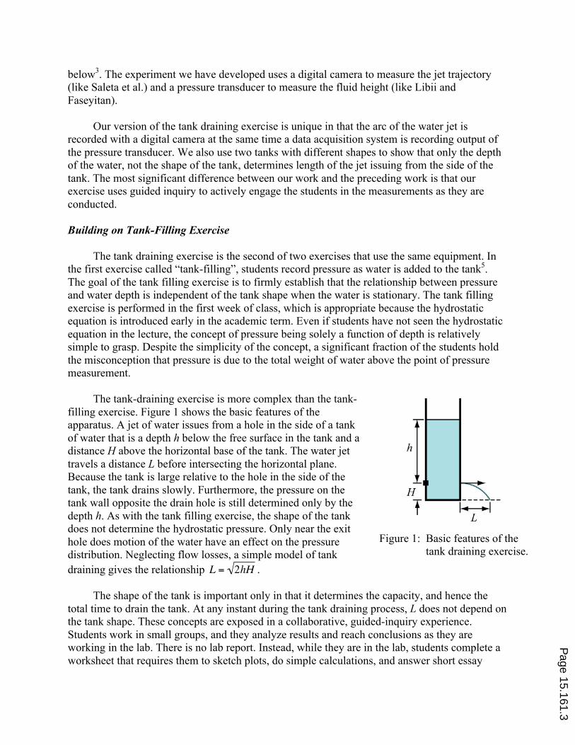
The tank-draining exercise is more complex than the tank-
filling exercise. Figure 1 shows the basic features of the
apparatus. A jet of water issues from a hole in the side of a tank
of water that is a depth h below the free surface in the tank and a
distance H above the horizontal base of the tank. The water jet
travels a distance L before intersecting the horizontal plane.
Because the tank is large relative to the hole in the side of the
tank, the tank drains slowly. Furthermore, the pressure on the
tank wall opposite the drain hole is still determined only by the
depth h. As with the tank filling exercise, the shape of the tank
does not determine the hydrostatic pressure. Only near the exit
hole does motion of the water have an effect on the pressure
distribution. Neglecting flow losses, a simple model of tank
draining gives the relationship L = 2hH .
The shape of the tank is important only in that it determines the capacity, and hence the
total time to drain the tank. At any instant during the tank draining process, L does not depend on
the tank shape. These concepts are exposed in a collaborative, guided-inquiry experience.
Students work in small groups, and they analyze results and reach conclusions as they are
working in the lab. There is no lab report. Instead, while they are in the lab, students complete a
worksheet that requires them to sketch plots, do simple calculations, and answer short essay
Figure 1: Basic features of the
tank draining exercise.
Page 15.161.3
Page 15.161.4

experiment was progressing. Each image was stored with a file name that indicated the time in
seconds from the start of the experiment. Capturing and storing the images on the fly was not
robust. The operating system (Windows XP) and LabVIEW would occasionally hang up,
requiring the experiment to be rerun, which caused the students to be frustrated.
A simpler and more robust solution is to asynchronously capture the images and then
transfer the images to the computer after the tank draining is complete. This approach requires a
mechanism for adding a time stamp to the images so that the L(t) measurement with the camera
can be associated with the h(t) measurement with the pressure transducer. A time stamp is added
to each image by positioning a six segment LED display kit (USB7 from Fundamental Logic
http://store.fundamentallogic.com) in the field of view of the camera. Figure 3 is a photograph of
a tank draining measurement in progress. An enlarged image of the LED is also inset in the
image. The digits on the LED display are set from the internal time of the LabVIEW program
recording the pressure transducer output. Therefore, each image that records L(t), also indicates
the time the image was captured according to the time base of the pressure measurements.
Figure 3. Stepped-tank during draining. The seven-segment LED display at the base of the
tank indicates the time in sections from the start of the pressure transducer
measurements. Blue food coloring was added to the water to increase the contrast.
Page 15.161.5

Data Collection and Analysis
In a conventional laboratory exercise, students record data in the lab and then go home to
analyze the data and write a report. In our guided inquiry exercise, the data collection and
analysis both happen in the laboratory. The objective is to engage students in reasoning while
they can change the sequence and configuration of the measurements. This requires students to
be more active participants in the laboratory. It also creates opportunities to practice qualitative
reasoning when students are asked to predict the outcome of a measurement and then confirm
that prediction with a measurement.
If analysis of measurement data is to occur in the laboratory, the analysis must either be
simple enough for students to do by hand in a short time, or the analysis must be supported by
software provided to the students. The latter approach is used in the tank draining exercise. The
pressure transducer data is recorded with a LabVIEW VI. Combination and analysis of the
pressure transducer and image data is performed with a MATLAB program provided to the
students.
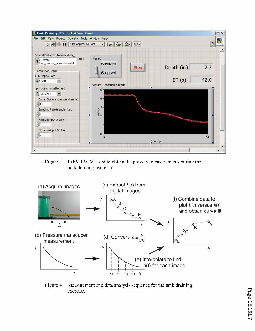
Figure 3 is a screen capture of the LabVIEW VI that records the pressure transducer output.
The center of the VI is a plot of the p(t) signal which is proportional to h(t). The “Depth” and
“ET” displayed in the upper right corner are the instantaneous water depth and the elapsed time.
The ET value is also sent to the LED display to provide the time stamp for the L(t) images. A
toggle switch on the VI determines which channel of the DAQ is stored in the data file. Two
pressure transducers – one for each of the two tanks – are connected to the DAQ. Therefore, the
toggle positions are labeled with “straight” or “stepped” to indicate the tank shape.
Each experiment with the tank draining apparatus consists of three main phases
1. Record output of the pressure transducer and capture images as water drains from the
tank.
2. Use an image viewer to assist in manually extracting the L(t) distance traveled by the jet.
3. Combine the h(t) and L(t) data to obtain L(h).
Figure 4 provides a more detailed conceptual map for the tasks involved in the data capture and
analysis. As the tank is draining, images are captured (step a.) and pressure versus time data is
recorded (step b). After the draining is complete and the data logging is stopped, the jet length
values, L, are extracted from the images captured by the digital camera (step c). The pressure
transducer values are converted to depth (step d). The time ti at which each image was captured
is used to interpolate in the depth versus time data, and to extract a set of h(ti) values
corresponding to each of the images used to measure L(ti), (step e). Finally, the L(ti) and h(ti)
data are combined to yield a plot of L(h), (step f). Figure 5 is an annotated screen shot of the
MATLAB program used to perform the analysis in steps d, e, and f.
Page 15.161.6
Page 15.161.7

Figure 5 Annotated screen shot of the user interface (UI) for the MATLAB
program that performs data analysis steps d, e, and f in Figure 4. The
data in the plots is from an experiment with the step-walled tank.
The analysis with the MATLAB program is performed in the following steps. The step
numbers correspond to the annotations in Figure 5.
1. The L(ti) data extracted from the images captured during the experiment are entered in a
spreadsheet-like data table. The ti are discrete times at which the images are captured. As
the L(ti) data is entered in the table, it is automatically displayed in the plot in the pane in
the upper right quadrant of the User Interface (UI) window.
2. The p(t) data captured by the LabVIEW VI is loaded from a text file saved by the VI.
The p(t) data is displayed in the figure pane in the lower right quadrant of the UI.
3. With the L(ti) data and p(t) stored in program memory, the user clicks a button labeled
“Transfer Jet Data”, which interpolates the p(t) data to find p(ti), i.e. the pressure at the
discrete times when then images of the water jet were captured. The p(ti) data is
converted to depth, h(ti), which is added to the data table in the upper left quadrant. To
visually represent the interpolation, short red vertical bars are added to the p(t) curve in
the lower right quadrant of the UI window. Page 15.161.8

4. With L(ti) and h(ti) data on a common time base ti, a plot of L(h) is created in the lower
left quadrant of the UI window.
5. The user clicks a button labeled “Add Curve Fit” and a least squares fit of L = c h is
performed and added to the L(h) plot. The value of c is displayed.
As a homework assignment or as part of a laboratory report, it would be reasonable to ask
students to perform the steps that are automated by the MATLAB program. In our guided inquiry
exercise, the computational tasks are automated, and the students are asked to provide reasoning
and explanations for the observed behavior.
Guided-Inquiry Exercise
As a result of performing the guided-inquiry exercise, students should achieve the
following learning objectives.
• Be able to apply mass conservation to a control volume with a time-varying mass;
• Be able to determine the pressure at depth in a tank with a small hole in its side;
• Use digital photographs to measure geometric features, specifically the trajectory of the
water jet emerging from a hole in the side of the tank;
• Apply the Bernoulli and Energy Equations to compute the velocity of a free jet emerging
from a hole in a tank;
• Explain the key similarities and key differences between the draining of two tanks with
different shapes.
Directions for performing the exercise are written in a worksheet that students complete in
the lab. There is no lab report. The calculations on the worksheet are simple enough to be
performed with a calculator. The MATLAB program depicted in Figure 5 performs the data-
intensive computations required to complete the exercise. Students make sketches of the plots
from the data analysis screens, and they are asked to predict how the trends in the plots will
change during the next set of experiments.
The exercise begins with both tanks filled with water. A complete cycle of measurement
and analysis is performed with the straight-walled tank. Worksheets provide a structured path of
inquiry. Questions are posed and the lab group is expected to reach conclusion before moving on
to the next phase of the measurements. The lab instructor is required to check the worksheet at
key points. The checkpoints are indicated by large “stop signs” in the worksheet. This prevents
students from rushing through the exercise in the way that they might in a typical lab exercise
that requires them only to record data.
All members of the team progress at the same pace. The goal is to encourage group
discussion and resolution of the conceptual questions. A modest amount of instructor
involvement is required to make this work. When the team has reached one of the stop signs, the
instructor can ask a conceptual question, and whether everyone agrees with the answer provided.
In Fall 2008 the tanks had only one size of drain hole. During a discussion with the
instructor, the effect of hole size was debated. In preparation for Fall 2009, the tanks were
Page 15.161.9

redesigned to have three drain holes 3.2 mm, 6.4 mm and 7.9 mm in diameter (1/8, 1/4 and 5/16
inch, respectively). The holes are at the same depth as the pressure transducer and are plugged
with corks. The tank base was redesigned to allow the tank to be rotated so that the water jet
emerging from hole can be aligned parallel with the horizontal meter stick. Only one hole is
opened at a time for each experiment. In the guided inquiry worksheet there is no explicit
instruction to choose a specific size of drain hole. At the start of the lab session, the instructors
position the tank so that the medium size hole is aligned to produce a water jet parallel to the
meter stick. The very last question on the guided inquiry worksheet is
Consider two straight-walled tanks that have holes with different diameters, say d1
and d2, with d1 > d2. At the same h, which tank would have the larger L? At the same
h, which tank would have the larger Vj?
The students are not instructed to obtain their answer with any measurements. The overwhelming
majority of student groups simply wrote down their opinion of the correct response. Only a small
number of student groups took advantage of the opportunity to make measurements to confirm
the answers to the last question on the worksheet.
Typical Results
In this section we show results from measurements with the tank draining apparatus. The
results are formatted for publication, and are not arranged exactly as the students see the results
from the MATLAB data reduction program during the laboratory exercise. However, the data is
obtained in the same way that students make measurements, and the data presented here was
recorded with the LabVIEW program used by students. Images used to obtain the L(t) data were
captured with a more expensive camera than that used by students, and extra care was taken to
align the camera to maximize accuracy of the L(t) measurements. Despite these modest
differences in procedure and equipment, students can obtain results similar, if not identical, to
those presented here.
Figure 6 shows representative data from the straight walled tank. The two plots on the left
side of the figure are measurements plotted as a function of time. The top plot is the output of the
pressure transducer, converted to depth. The bottom plot is the jet length data obtained from
inspection of the digital images. During draining, the changes in depth and the variation in jet
length are smoothly varying functions of time. The plot on the right has eliminated time to plot L
as a function of h. A curve fit of L = c h , where c is a constant, is a good match to the data.
During the laboratory exercise, students see the data displayed as in Figure 5 (without the
numbered circles). They are asked to sketch the h(t), L(t) and L(h) plots on their worksheets.
Before making measurements on the step-walled, tank, students are asked to overlay sketches of
their predictions for the h(t), L(t) and L(h) data from the step-walled tank. Students then perform
the experiment on the step-walled tank to confirm or reject their prediction. Figure 7 shows
representative data from the step walled tank. The plots on the left of the time-varying data show
a distinct kink at the time when the water depth crosses the change in tank diameter. Although
the time varying data shows clear evidence of the influence of the step change in area, the L(h)
data is smooth.
Page 15.161.10

Figure 6 Data from draining of the straight-walled tank. On the left are the h(t)
and L(t) curves (top and bottom, respectively). On the right is the
combined L(h) data and the curve fit of L = c h to that data.
Figure 7 Data from draining of the step-walled tank. On the left are the h(t) and
L(t) curves (top and bottom, respectively). On the right is the
combined L(h) data and the curve fit of L = c h to that data.
Page 15.161.11
Having performed the experiment on the straight-walled tank and the step-walled tank, the
natural question is how do these tanks compare. Figure 8 is a plot of the L(h) data for the
straight-walled tank and the step-walled tank when water is draining from the medium sized
hole. The two L(h) data sets are very close. The difference in the L(h) data is due to
manufacturing tolerances in the holes, which causes slight differences in the loss coefficients.
The most important information from Figures 6, 7 and 8 is that the L(h) function is
independent of the tank geometry. The guided inquiry worksheet begins with a theoretical
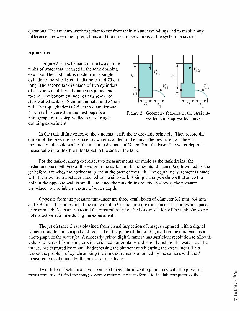
analysis of the tank draining problem and a short derivation shows that L = 2Hh , where H is
the height of the hole above the horizontal plane that defines L (see Figures 1 and 2). Students
are given the worksheets in advance, and they are told to study the first few pages before coming
to the lab. The significance of the simple L = 2Hh is reinforced by the measurements.
Another natural question is how does the hole size affect the jet velocity and travel length.
Figure 9 shows the measurements L(h) on the step-walled tank for drain holes, 3.2 mm, 6.4 mm
and 7.9 mm in diameter. The L(h) curves for the medium and large holes are close to each other.
The small hole is distinctively lower. The jet of water from the small hole is qualitatively
different from the jet of water from the larger holes. The jet from the small hole is not round and
has a wavy instability. We suspect that the dynamics of the jet after it has left the tank is unlikely
to affect the distance traveled by the jet. Rather, we believe that the loss coefficient of the
smaller hole is larger than the loss coefficient from the larger holes.
Conclusion
The tank draining apparatus is relatively inexpensive and its operation is easily
comprehendible to students. The apparatus is used in two exercises: one focused simply on the
hydrostatic equation, and one involving the draining experiment described in this paper. The
apparatus also provides an opportunity to engage students in guided-inquiry pedagogy. The first
exercise is simple and has the objective of introducing the students to inquiry-based laboratory
work. The second exercise is more subtle. It requires students to transform measurements made
in real time – p(t) and L(t) – into the more fundamental relationship L = f(h).
Within a two-hour lab session, students can observe and characterize the behavior of the
straight-walled tank. From those observations they can predict the behavior of the tank with a
cross section that varies with depth. This exercise confirms the hydrostatic equation and extends
it to the situation of measuring the depth in a slowly draining tank.
As with any teaching experience, many factors influence on the learning outcomes from the
tank draining exercise. We have refined the apparatus and the worksheets over two years. The
procedures are robust and can be used at other universities. We encourage instructors to visit
eet.cecs.pdx.edu. There they will find the latest copy of the guided-inquiry worksheet, and more
details on the experimental apparatus.
Page 15.161.12

Figure 8 Combined L(h) data for the straight-walled and step-walled tanks with
medium-size drain holes.
Figure 9 Effect of hole size on the L(h) data for the step-walled tank.
Page 15.161.13

Acknowledgement
This work is supported by the National Science Foundation under Grant No. DUE
0633754. Any opinions, findings, and conclusions or recommendations expressed in this material
are those of the authors and do not necessarily reflect the views of the National Science
Foundation.
The authors are grateful for the assistance of Dr. Jack Kirschenbaum in interpreting the
survey data. The authors are also very appreciative of the cooperation and support of Dr. Derek
Tretheway who taught the lecture section of EAS 361 during Fall 2008 and Fall 2009. Jerimiah
Zimmerman was very helpful as the teaching assistant in Fall 2009. Michael Chuning redesigned
and fabricated the two tanks used in the exercises.
References
1. Libii, J.N., Mechanics of the slow draining of a large tank under gravity. American Journal
of Physics, 2003. 71(11): p. 1204-1207.
2. Libii, J.N. and S.O. Faseyitan. Data acquisition systems in the fluid mechanics laboratory:
Draining of a Tank. in 1997 ASEE Annual Conference and Exposition Year. Milwaukee,
WisconsinASEE.
3. Saleta, M.E., D. Tobia, and S. Gil, Experimental study of Bernoulli's equation with losses.
American Journal of Physics, 2005. 73(7): p. 598-602.
4. Munson, B.R., D.F. Young, and T.H. Okiishi, Fundamentals of Fluid Mechanics. fifth ed.
2006, New York: Wiley.
5. Edwards, R., G. Recktenwald, and B. Benini. A laboratory exercise to teach the hydrostatic
principle as a core concept in fluid mechanics. in ASEE Annual Conference and
Exposition. Austin, TX. June 14-17, 2009, American Society for Engineering Education.
Page 15.161.14