Citation: Underwood, Chris (2014) An improved lumped parameter method for building thermal modelling. Energy and Buildings, 79. pp. 191-201. ISSN 0378-7788

Published by: Elsevier

URL: http://dx.doi.org/10.1016/j.enbuild.2014.05.001 <http://dx.doi.org/10.1016/j.enbuild.2014.05.001>

This version was downloaded from Northumbria Research Link: http://nrl.northumbria.ac.uk/16866/

Northumbria University has developed Northumbria Research Link (NRL) to enable users to access the University’s research output. Copyright ©  and moral rights for items on NRL are retained by the individual author(s) and/or other copyright owners. Single copies of full items can be reproduced, displayed or performed, and given to third parties in any format or medium for personal research or study, educational, or not-for-profit purposes without prior permission or charge, provided the authors, title and full bibliographic details are given, as well as a hyperlink and/or URL to the original metadata page. The content must not be changed in any way. Full items must not be sold commercially in any format or medium without formal permission of the copyright holder. The full policy is available online: http://nrl.northumbria.ac.uk/policies.html

This document may differ from the final, published version of the research and has been made available online in accordance with publisher policies. To read and/or cite from the published version of the research, please visit the publisher’s website (a subscription may be required.)

1

An improved lumped parameter method for building thermal modelling

C. P. Underwood

Faculty of Engineering and Environment, University of Northumbria, UK

Abstract

In this work an improved method for the simplified modelling of the thermal response of

building elements has been developed based on a 5-parameter second-order lumped

parameter model. Previous methods generate the parameters of these models either

analytically or by using single objective function optimisation with respect to a reference

model. The analytical methods can be complex and inflexible and the single objective

function method lacks generality. In this work, a multiple objective function optimisation

method is used with a reference model. Error functions are defined at both internal and

external surfaces of the construction element whose model is to be fitted and the resistance

and capacitance distributions are adjusted until the error functions reach a minimum.

Parametric results for a wide range (45) of construction element types have been presented.

Tests have been carried out using a range of both random and periodic excitations in weather

and internal heat flux variables resulting in a comparison between the simplified model and

the reference model. Results show that the simplified model provides an excellent

approximation to the reference model whilst also providing a reduction in computational cost

of at least 30%.

Keywords:

Dynamic thermal modelling; building response; lumped parameter modelling; optimisation

Corresponding author: Tel +44-191-227-3533 Email: chris.underwood@northumbria.ac.uk

List of symbols

A Area (m2)

C Thermal capacity per unit area (Jm-2

K-1

)

c Specific heat capacity (Jkg-1

K-1

)

F Fourier number

f Thermal resistance rationing factor

g Thermal capacity rationing factor

h Surface convection coefficient (Wm-2

K-1

)

k Thermal conductivity (Wm-1

K-1

)

L Number of layers of material

m Mass flow rate (kgs-1

)

Q Heat transfer (W)

R Thermal resistance (m2KW

-1)

T Temperature (oC, K)

T Sol-air temperature (external), rad-air temperature (internal) (oC)

t Time (s)

W Weighting factor

x Distance (m)

2

Greek

α Thermal diffusivity (m2s

-1 = k / c)

t Time step increment (s)

x Spatial increment (m)

ε Root-mean-square error

Density (kgm-3

)

ΣC Total element thermal capacity per unit area (Jm-2

K-1

)

ΣR Total element thermal resistance (m2KW

-1)

Subscripts and superscripts

a Air, material ref. ‘a’

b Material ref. ‘b’

c Convection

i Layer node index

i Internal (space)

m Middle position

n Time row index

o Outside, exterior

r Radiant, solar radiation

s Surface

s Surface index number

upper Upper bound limit

1. Introduction

In 2002 Gouda et al. [1] developed a simplified method for the dynamic thermal modelling of

single-layer and multi-layer construction elements. They used an optimisation algorithm to

find the five required parameters of the simplified model by matching its dynamic response to

a high-order reference model. The work was limited in three respects:

A unit step response was used as the excitation variable for the simplified model

parameter fitting whereas excitations in practice vary continuously.

The results were based on excitations applied individually to both heat flux and

temperature at one surface only using a single objective function search algorithm

whereas in practice, both internal and external surfaces would be subject to

simultaneous excitations of more than one variable.

Only two sets of results were published making it difficult for other users to make

use of the simplified model.

In this work an improved method is proposed for the extraction of the simplified model

parameters based on a multiple objective function search algorithm (i.e. objective functions

simultaneously applied to both inside and outside surfaces) and the use of a reference model

consisting of a rigorous finite-difference method. Extensive sets of results are generated for a

range of common construction elements and a sample of these elements are tested in the

context of a simple room enclosure model which alternately uses the simplified model and

the more rigorous reference model for its construction elements.

3

2. Review

The application of lumped parameter modelling methods to building dynamic thermal

response is motivated by the desire to find simpler and, hence, computationally less

‘expensive’ methods for the analysis building thermal energy response. Approaches broadly

fall into two categories:

Lumped parameter construction element models from which whole room models may

be constructed [1, 2, 3]

Lumped parameter whole room models [4, 5, 6, 7, 8]

Though the differences between the two approaches are rather subtle (since models of

individual constructions elements are almost always used as a basis for grouping or

aggregating into whole room models), the treatment of individual elements usually provide

greater detail in modelling information such as individual surface temperatures which can be

important when dealing with radiant sources, etc.

Lorenz and Masy [2] were among the first to propose a simplified lumped parameter

approach to building response modelling using a first-order model consisting of two

resistances and one capacitor. Gouda et al. [1] demonstrated improved accuracy using a

second-order model in which each construction element is described using three resistances

and two capacitances. These approaches to modelling were often referred to as ‘analogue

circuit’ models due to their connotation with electric circuits (i.e. see Figure 1 in Section 4).

Fraisse et al. [3] also compared first- and second-order element models (the latter referred to

as a ‘3r2c’ model) and went further to propose a fourth-order ‘3r4c’ model with aggregated

resistances. Like Lorenz and Masy [2], they propose an analytical method for deriving the

parameters of the model (essentially, the distribution of resistance and capacitance values

throughout the ‘circuit’) whereas Gouda et al. [1] used an optimisation method to determine

the parameters with reference to a rigorous reference model.

Crabb et al. [4], Tindale [5] and others [6, 7, 8] have applied the lumped parameter approach

to the formulation of low-order whole room models by casting the capacitance parameter

over the higher capacity elements of a room (external walls, solid floors, etc) and using

algebraic heat balances for the lower capacity room elements (demountable partitions, etc).

Tindale [5] attempted this using a second-order room model but found that it provided

unacceptable results for rooms with very high thermal capacity (i.e. ‘traditional’

construction). He corrected this by introducing a third ‘equivalent’ room capacitance which

required an inconvenient method for its parameterisation.

Though low-order whole room models offer very low computational demands and simplicity,

there remain questions over the accuracy of these models particularly over long time horizons

and they tend to provide less modelling information (i.e. individual and accurate element

surface temperatures) essential in many lines of design enquiry. For this reason, it is argued

that room models constructed from second-order (or higher) construction element

descriptions provide greater accuracy and detail whilst retaining some of the key advantages

4

of simplicity and low computational demand and are, therefore, to be preferred other than for

approximate and early feasibility simulation studies.

The key advantages of lumped parameter building modelling are those of simplicity,

transparency and low computational demand. They are particularly suited to bespoke (i.e.

research-based) building response modelling using either modular-graphical modelling tools

such as Simulink [9] – see for example [10, 11, 12], or equation-based methods such as

Modelica [13] or EES [14, 15].

3. Reference Conduction Model

A key requirement for accuracy in simplified lumped parameter building models is the

correct distribution of the overall element resistance and capacitance to ensure that the

element surface temperatures are accurately predicted. It is possible to attempt this

analytically as has been done by Lorenz and Masy [2] and Fraisse [3] however these methods

usually require complicated mathematical models and are often restricted to defined surface

input excitations. In the present work, an optimisation procedure is designed to adjust the

resistance and capacitance distributions so that the surface temperature of the simplified

model matches that of a rigorous reference model.

The reference construction element model was created from the one-dimensional energy

equation using a finite-difference scheme:

2

2

T T

t x

(1)

A full description of the discretisation and solution procedure of this equation as adopted in

the present work applied to multi-layer construction elements can be found in [16]. A

summary of the main discretised equations is given in the following for reference. For the

temperature distribution through the body of each layer of material the following is used

where the superscript n refers to the current time row and n+1 to the next time row:

1 1 11 1

1

2 1

n n n ni i i iT T FT FT

F

(2)

in which the Fourier number, F, can be shown to be:

2

tF

x

(3)

At the interfaces between two differing layers of material the interface temperature is

obtained from the following (expressed here as the interface centred at the ith

discrete slice

forming a junction between two layers of different material, ‘a’ and ‘b’):

5

1 1 1 11 11

a ba a a b b b a b

2n n n n

i i i in ni i

T T T TtT T k k

c x c x x x

(4)

And at a surface boundary, the temperature of the first discrete slice of the first layer of

material is given by the following (in this case for the first slice of material on the inside

surface layer which is taken to form slice 1 and bounded by room air at Ti with a surface

convection coefficient of hi):

1 1 1 11 2 i 11

1 1 ii1 / 2

n n n n

n nT T T Tt

T T k hc x x h x k

(5)

Finally, the temperature at the inside surface (of zero heat capacity) will be:

1 11 i i1

si

/ 2

1 / 2

n nn T T h x k

Th x k

(6)

(a similar equation can be written for the temperature of the exterior surface).

The reference model was solved using a fully implicit scheme adopting Gauss-Seidel

iteration. The discretisation scheme adopted one node at the centre of each layer of material

and thus, with the interface equations, 2L+1 conduction equations needed to be solved

iteratively at each time step (where L is the number of layers of material) plus the two surface

temperature equations.

4. Second-order Lumped Parameter Model

A simplified second-order construction element model can be used as an approximation to

the much more rigorous description of the previous section. Gouda et al. [1] compared both

first-order and second-order simplifications and concluded that the latter was an improvement

on the former in terms of accuracy whilst requiring little additional computational effort.

Figure 1 illustrates the parameters and variables of the second-order model based generally

on that of Gouda et al. [1].

6

Figure 1 – Simplified 2nd

-order construction element model

The overall thermal resistance between the inside and outside surfaces, ΣR (m2KW

-1), can be

easily calculated from material properties as can the overall thermal capacity per unit area,

ΣC (Jm-2

K-1

). To generate the simplified model, the overall surface-to-surface resistance

requires to be apportioned between the three series resistances, Ri, Rm and Ro, and the overall

thermal capacity requires to be apportioned between the two capacitances, Ci and Co such

that:

i i

o o

m i o m i o

i i

o i o i

1

1

R f R

R f R

R R R R f f f

C g C

C C C g g

(7)

(8)

(9)

(10)

(11)

Gouda et al. [1] referred to fi, fo, fm, gi and go as resistance and capacitance rationing factors.

Thus a second-order model for a multi-layered construction element can be realised as

follows.

ii ai i i o

i si i o

oi i o o ao

i o o so

d 1 1

d 1

d 1 11

d 1

Tg C T T T T

t f R R f f R

Tg C T T T T

t f f R f R R

(12)

(13)

And the internal and external surface temperatures using this model will be:

7

i ai si isi

i si

o ao so oso

o so

R T R TT

R R

R T R TT

R R

(14)

(15)

This model can be completely parameterised by obtaining values for the three resistance and

capacitance rations fi, fo and gi.

In the original study, Gouda et al. [1] developed three alternative complete room models.

The first used construction elements based on a high-order reference model. The second used

the simplified second order model for the construction elements and the third used an existing

first order model for comparative purposes. A single objective function search algorithm was

applied to find values of the three rationing parameters which minimised the root-sum-

square-error in the room air temperatures predicted by the second-order model and the

reference model in response to a unit step change in either heat flux at the external surface

(e.g. due to solar radiation) or external air temperature. The method and results given in this

original study were limited in a number of respects:

A whole room model was used to generate the parameter values making it

difficult for the work to be replicated by other researchers and practitioners.

A step response excitation for this application is unrealistic.

The method would require to be repeatedly applied for different disturbance

variables and is inapplicable when more than one excitation variable are

simultaneously active.

There was an insufficient number of results for alternative construction types

making it difficult to utilise the model for a range of alternative applications.

The method and results reported in the following sections attempt to address these

shortcomings in the following ways:

a) A multiple objective function search algorithm is used with simultaneous disturbances

applied to both inside and outside surfaces of the reference and target models.

b) The proposed new method is applied at the construction element level by targeting

surface (rather than room) temperatures thus making the method easier to replicate by

other researchers and practitioners.

c) The method is tested at room level in relation to room temperature response to

demonstrate robustness.

d) A periodic function is used to drive the excitation variables.

e) A large number of results are generated and reported for a range of alternative

construction elements making the model easy for students, researchers and

practitioners to apply without needing to carry out a parameter-fitting analysis.

8

5. Optimised Parameter Fitting Method

A function was created to implement the two models described in sections 4 and 5 for a

defined single or multi-layer construction element. The internal and external air temperatures

were varied sinusoidally with peak-to-peak amplitudes of 1K and a period of 24h consistent

with a diurnal cycle. The internal and external surface temperatures predicted by eqns. (6)

(reference model), and eqns. (14 & 15) (second-order model) were obtained and root-mean-

square error values between the two sets of surface temperatures (si so

,T T for the internal

and external surface errors respectively) were returned as a function of values of the three

rationing parameters, fi, fo and gi. The followuing optimisation problem was then set up:

si so

si soi o i

i o i, ,

i o i i-upper, o-upper i-upper

,

min , subject to: , , 0,0,0

, , , ,

T T

T Tf f g

W W Goal

f f g

f f g f f g

(16)

An active-set optimisation algorithm was used with a single objective function derived from

an importance weighting of the two fundamental objective functions, si so

,T T . Unity

weightings were applied to both of the root objective functions in the work reported here to

signify that both internal and external surface temperature targets were equally important. (In

practice, the Matlab function ‘fgoalattain’ was used for the above [17].)

6. Improved Second-order Lumped Parameter Model – Results

The optimisation algorithm was applied to a wide range of typical construction elements

grouped into 4 categories:

Internal partitions (14 examples)

Floors (8 examples)

Roofs (8 examples)

External walls (15 examples)

The overall surface-to-surface resistances (including allowances for interstitial air gaps where

relevant) and overall thermal capacities were calculated using material properties listed in

CIBSE Guide, Book A [18].

Results for the various construction elements are given in the tables in Appendix A. The

tables list the resistance rations (internal zone, middle and outer zone) and capacitance rations

(internal zone and outer zone) so that the simplified lumped parameter construction element

model described in Section 4 can be fully parameterised for any chosen element. As might

be expected, for single layer elements or multi-layer elements with symmetrical layering, the

9

results show that fi = fo and gi = go = 0.5. For multi-layer elements with many layers (e.g. >4)

the middle zone resistance tends to dominate.

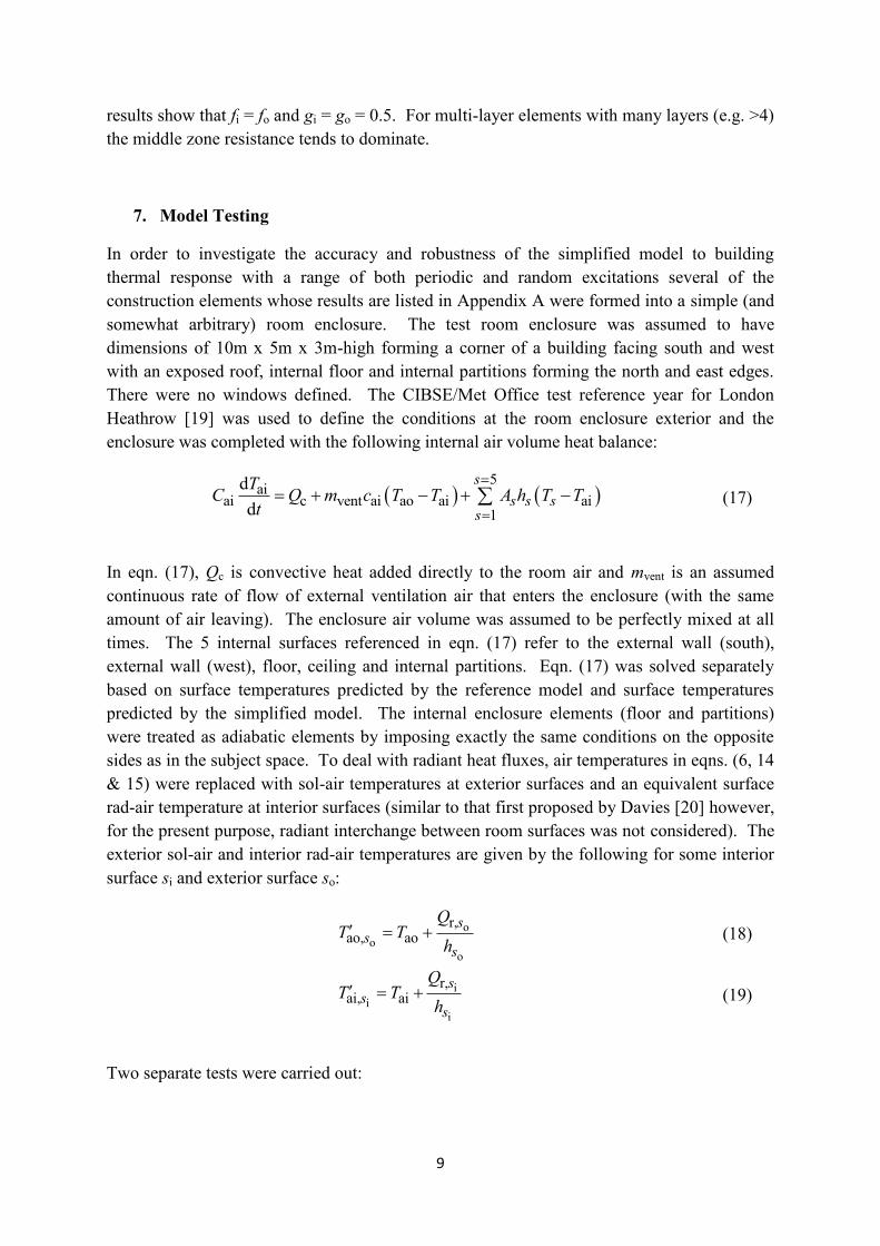
7. Model Testing

In order to investigate the accuracy and robustness of the simplified model to building

thermal response with a range of both periodic and random excitations several of the

construction elements whose results are listed in Appendix A were formed into a simple (and

somewhat arbitrary) room enclosure. The test room enclosure was assumed to have

dimensions of 10m x 5m x 3m-high forming a corner of a building facing south and west

with an exposed roof, internal floor and internal partitions forming the north and east edges.

There were no windows defined. The CIBSE/Met Office test reference year for London

Heathrow [19] was used to define the conditions at the room enclosure exterior and the

enclosure was completed with the following internal air volume heat balance:

5

aiai c vent ai ao ai ai

1

d

d

s

s s ss

TC Q m c T T A h T T

t

(17)

In eqn. (17), Qc is convective heat added directly to the room air and mvent is an assumed

continuous rate of flow of external ventilation air that enters the enclosure (with the same

amount of air leaving). The enclosure air volume was assumed to be perfectly mixed at all

times. The 5 internal surfaces referenced in eqn. (17) refer to the external wall (south),

external wall (west), floor, ceiling and internal partitions. Eqn. (17) was solved separately

based on surface temperatures predicted by the reference model and surface temperatures

predicted by the simplified model. The internal enclosure elements (floor and partitions)

were treated as adiabatic elements by imposing exactly the same conditions on the opposite

sides as in the subject space. To deal with radiant heat fluxes, air temperatures in eqns. (6, 14

& 15) were replaced with sol-air temperatures at exterior surfaces and an equivalent surface

rad-air temperature at interior surfaces (similar to that first proposed by Davies [20] however,

for the present purpose, radiant interchange between room surfaces was not considered). The

exterior sol-air and interior rad-air temperatures are given by the following for some interior

surface si and exterior surface so:

o

o

o

i

i

i

r,ao, ao

r,ai, ai

ss

s

ss

s

QT T

h

QT T

h

(18)

(19)

Two separate tests were carried out:

10

A moderately high thermal capacity test using external wall type 6 (Appendix A,

Table A1.4), roof type 5 (Appendix A, Table A1.3), floor type 5 (Appendix A, Table

A1.2) and partition type 9 (Appendix A, Table A1.1) giving an overall enclosure

fabric thermal capacity of 48.9MJK-1

.

A low thermal capacity test using external wall type 2 (Appendix A, Table A1.4), roof

type 3 (Appendix A, Table A1.3), floor type 1 (Appendix A, Table A1.2) and

partition type 1 (Appendix A, Table A1.1) giving an overall enclosure fabric thermal

capacity of 6.8MJK-1

.

The tests consisted of one complete annual simulation in each case, using the weather file.

The global horizontal solar radiation in the weather file was first pre-processed into annual

time-series surface irradiances relevant to the south- and west-facing walls and the horizontal

roof surface using the clearness index model of Skartveith and Olseth [21]. A ground

reflection factor of 0.2 was assumed and a surface absorption coefficient of 0.9 was used for

all surfaces. The results were then used in eqn. (18) to determine time-series sol-air

temperatures for each surface together with the corresponding external air temperature from

the weather data.

mvent was calculated by assuming a constant rate of ventilation equivalent to 0.5 of an air

change per hour. An internal heat excitation rate of 1kW (20Wm-2

of floor area) was ramped

in each day of the simulation between 07:00h and 10:00h and then ramped back down to zero

between 18:00h and 21:00h after being held constant between these times. Half of this

energy was allocated to convection (entering via the Qc term in eqn. (17)) and the remaining

half was uniformly added to each surface as radiation (entering via the rad-air temperatures of

eqn. (19)).

Though the conditions defined above are somewhat arbitrary, they are considered sufficient

to capture a wide range of the important variables that are likely to be of primary influence

over the behaviour of a construction fabric dynamic thermal model.

Results of the two tests are presented in the following. They were obtained using an

integration time step of 1 minute over one complete annual cycle. The reference model used

a single central node for each layer of material such that each layer of material was

completely defined by 3 nodes (one at the centre and two interface nodes). Thus 2L+1

equations (where L is the number of material layers) required to be solved for the reference

model whereas just 2 equations require to be solved for all instances of the simplified model

(excluding surface equations in both cases).

Comparisons of the enclosure air temperature predicted by both models are given in figures 2

and 3. Figure 2 shows that the simplified model gives an excellent agreement with the

reference model for a traditional high thermal capacity construction. Figure 3 shows that the

agreement is adequate for a low thermal capacity construction though not as good as for high

thermal capacity. This conclusion is also evident in the results of surface temperature

comparison shown in Figure 4 (high thermal capacity) and Figure 5 (low thermal capacity).

The surface temperature comparisons show a good level of agreement over a very wide range

11

of operating surface temperatures particularly the exterior surfaces of the external wall and

roof where solar radiation is responsible for some high surface temperature behaviour.

Figure 2 – Enclosure air temperature comparisons (high thermal capacity)

(Top: Three day sample, winter / Middle: Three day sample, summer / Bottom: All data)

Figure 3 – Enclosure air temperature comparisons (low thermal capacity)

(Top: Three day sample, winter / Middle: Three day sample, summer / Bottom: All data)

12

Figure 4 – Fabric surface temperature agreements (high thermal capacity)

Figure 5 – Fabric surface temperature agreements (low thermal capacity)

The overall RMS error results are given in Table 1. The overall average RMS errors

resulting from the two models over all surface temperatures and the internal air temperature

are 0.30K (high thermal capacity) and 0.43K (low thermal capacity).

13

Table 1 – RMS errors in key variables between the reference and simplified models

Variable High thermal capacity test Low thermal capacity test

Air temperature 0.24 0.50

External wall (south) inside

surface temperature

0.25 0.43

External wall (south) outside

surface temperature

0.18 0.11

External wall (west) inside

surface temperature

0.25 0.43

External wall (west) outside

surface temperature

0.18 0.11

Internal floor inside surface

temperature

0.38 0.66

Internal floor opposite

surface temperature

0.32 0.57

Ceiling surface temperature 0.29 0.53

Roof outside surface

temperature

0.74 0.22

Partition inside surface

temperature

0.22 0.59

Partition opposite surface

temperature

0.22 0.59

Mean over all variables 0.30 0.43

The computational elapsed time using the reference model only was 9.1 minutes (high

thermal capacity test case) and 9.8 minutes (low thermal capacity test case). When using the

simplified model only, the computational elapsed time reduced to 6.5 minutes (both cases) –

a reduction of around 30%.

Results were also generated using alternative integration time intervals of 5 minutes and 10

minutes (the default time step used in a number of commercially available energy simulation

programs). The RMS errors did not change significantly at these wider time steps. To a

certain extent this is to be expected since the conduction calculations are performed using an

implicit calculation algorithm (though at very wide time steps the accuracy would be

expected to begin to suffer). However the computation times reduced to an average of 2.6

minutes (reference model) and 1.3 minutes (simplified model) at an integration interval of 5

minutes and an average of 1.6 minutes (reference model) and 0.7 minutes (simplified model)

at the higher integration time step.

8. Comparisons with Established Methods

The advantages of the simplified building element model developed in this work are those of

simplicity, transparency and ease of implementation compared with established methods.

Though not suited to rigorous detailed simulations of multi-zone buildings, the simplified

14

method is particularly suited to smaller (e.g. 1-3 zone) building response modelling using

modular-graphical or equation-based modelling tools as are frequently used in building

energy research or in bespoke building design practice. The model developed here has been

fitted to a range of building element thermal responses generated using a detailed finite-

difference numerical model. The finite-difference numerical method for conduction

calculations is used in several established energy simulation tools including ‘ApacheSim’

which forms part of IES, the predominant energy simulation program used by practitioners in

the UK [22], and ‘ESP-r’ which is a long-standing freeware-based energy simulation program

used mainly by researchers [23]. However, arguably the dominant method of performing

these calculations is through the use of conduction transfer functions which are used in many

of the early simulation programs such as ‘BLAST’ and ‘DOE-2’ and, more recently, a very

widely used program which was formed out of these two called ‘EnergyPlus’ [24].

In order to explore the performance of the simplified model developed in this work with the

use of the conduction transfer function (CTF) method, a further simple test was conducted.

An example cooling load transient performed using CTFs on a 5-layer external wall

construction with defined internal and external surface temperatures was described by Spitler

[25]. Details of the data used, and the transient cooling load results obtained, are given in

Appendix 2. The optimisation method described in Section 5 was applied to Spitler’s

example construction using the finite-difference reference model described in Section 3 and

the following results were obtained for the simplified lumped parameter model:

fi = 0.100 ; fm = 0.866 ; fo = 0.034 ; gi = 0.360 ; go = 0.640

The simplified model was then applied using the above parameter settings and Spitler’s

surface temperatures [25] as listed in Appendix 2. The results of internal cooling load surface

heat fluxes are compared in Figure 6. The root-mean-square error between Spitler’s results

[25] and the simplified model was found to be 0.0286 (i.e. < 3%). Thus the simplified model

fitted using a finite-difference reference model appears to offer a very good approximation to

the traditional CTF conduction modelling method.

Figure 6 – Simplified and CTF model response comparison of surface heat flux transient

15

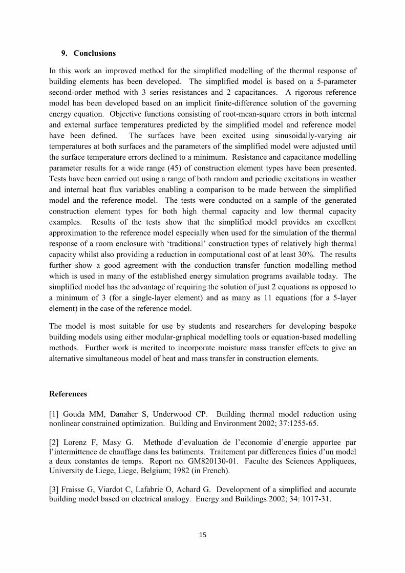
9. Conclusions

In this work an improved method for the simplified modelling of the thermal response of

building elements has been developed. The simplified model is based on a 5-parameter

second-order method with 3 series resistances and 2 capacitances. A rigorous reference

model has been developed based on an implicit finite-difference solution of the governing

energy equation. Objective functions consisting of root-mean-square errors in both internal

and external surface temperatures predicted by the simplified model and reference model

have been defined. The surfaces have been excited using sinusoidally-varying air

temperatures at both surfaces and the parameters of the simplified model were adjusted until

the surface temperature errors declined to a minimum. Resistance and capacitance modelling

parameter results for a wide range (45) of construction element types have been presented.

Tests have been carried out using a range of both random and periodic excitations in weather

and internal heat flux variables enabling a comparison to be made between the simplified

model and the reference model. The tests were conducted on a sample of the generated

construction element types for both high thermal capacity and low thermal capacity

examples. Results of the tests show that the simplified model provides an excellent

approximation to the reference model especially when used for the simulation of the thermal

response of a room enclosure with ‘traditional’ construction types of relatively high thermal

capacity whilst also providing a reduction in computational cost of at least 30%. The results

further show a good agreement with the conduction transfer function modelling method

which is used in many of the established energy simulation programs available today. The

simplified model has the advantage of requiring the solution of just 2 equations as opposed to

a minimum of 3 (for a single-layer element) and as many as 11 equations (for a 5-layer

element) in the case of the reference model.

The model is most suitable for use by students and researchers for developing bespoke

building models using either modular-graphical modelling tools or equation-based modelling

methods. Further work is merited to incorporate moisture mass transfer effects to give an

alternative simultaneous model of heat and mass transfer in construction elements.

References

[1] Gouda MM, Danaher S, Underwood CP. Building thermal model reduction using

nonlinear constrained optimization. Building and Environment 2002; 37:1255-65.

[2] Lorenz F, Masy G. Methode d’evaluation de l’economie d’energie apportee par

l’intermittence de chauffage dans les batiments. Traitement par differences finies d’un model

a deux constantes de temps. Report no. GM820130-01. Faculte des Sciences Appliquees,

University de Liege, Liege, Belgium; 1982 (in French).

[3] Fraisse G, Viardot C, Lafabrie O, Achard G. Development of a simplified and accurate

building model based on electrical analogy. Energy and Buildings 2002; 34: 1017-31.

16

[4] Crabb JA, Murdoch N, Penman JM. A simplified thermal response model. Building

Services Engineering Research and Technology 1987; 8: 13-9.

[5] Tindale A. Third-order lumped-parameter simulation method. Building Services

Engineering Research and Technology 1993; 14(3): 87-97.

[6] Nielsen TR. Simple tool to evaluate energy demand and indoor environment in the early

design stages. Solar Energy 2005; 78: 73-83.

[7] Kämpf JH, Robinson D. A simplified thermal model to support analysis of urban

resource flows. Energy and Buildings 2007; 39: 445-53.

[8] Antonopoulos KA, Koronaki EP. On the dynamic thermal behaviour of indoor spaces.

Applied Thermal Engineering 2001; 21: 929-40.

[9] SIMULINK Simulation and model-based design. Available at:

http://www.mathworks.co.uk/products/simulink/ [Accessed: 12 July 2013.]

[10] Henze GP, Neumann C. Building Performance Simulation for Design and Operation

(eds. Hensen JLM, Lamberts R). London: Spon Press; 2011, Chapter 14, p. 436-40.

[11] SIMBAD building and HVAC modelling toolbox for Matlab/Simulink. Available at:

http://www.simbad-cstb.fr/ [Accessed: 12 July 2013.]

[12] Kalagasidis AS et al. The International Building Physics Toolbox in Simulink. Energy

and Buildings 2007; 39: 665-74.

[13] Modelica – A unified object-oriented language for physical systems. Available at:

http://www.modelica.org/documents/ModelicaSpec32.pdf [Accessed: 12 July 2013.]

[14] F_Chart software: EES – Engineering Equation Solver. Available at:

http://www.fchart.com/ees [Accessed: 12 July 2013.]

[15] Bertagnolio S, Lebrun J. Simulation of a building and its HVAC system with an

equation solver: Application to benchmarking. Building Simulation 2008; 1: 234-50.

[16] Underwood CP, Yik FWH. Modelling Methods for Energy in Buildings. Oxford:

Wiley-Blackwell; 2004, p. 47-56.

[17] Mathworks documentation centre – fgoalattain. Available at:

http://www.mathworks.co.uk/help/optim/ug/fgoalattain.html [Accessed: 5 July 2013.]

[18] CIBSE Guide Book A Section A3 – Thermal Properties of Building Structures (5th

edition). London: Chartered Institution of Building Services Engineers; 1988, Table A3.15,

pA3-22.

[19] Weather data and climate change information. London: Chartered Institution of

Building Services Engineers. Available at:

http://www.cibse.org/index.cfm?go=page.view&item=1300 [Accessed: 7 July 2013.]

17

[20] Davies MG. Rad-air temperature: The global temperature in an enclosure. Building

Services Engineering Research & Technology 1989; 10(3): 89-104.

[21] Skartveit A, Olseth JA. A model for the diffuse fraction of hourly global radiation.

Solar Energy 1987; 38(4): 271-4.

[22] ApacheSim Calculation Methods. Glasgow: Integrated Environmental Solutions Ltd.

Available at:

http://www.iesve.com/downloads/help/Thermal/Reference/ApacheSimCalculationMethods.p

df [Accessed: 16 January 2014.]

[23] Clarke JA. Energy Simulation in Building Design. Oxford: Butterworth Heinemann;

2001, Appendix G, p. 355-6.

[24] EnergyPlus Energy Simulation Software – EnergyPlus Documentation. USA

Department of Energy. Available at:

http://apps1.eere.energy.gov/buildings/energyplus/energyplus_documentation.cfm [Accessed:

16 January 2014.]

[25] Spitler JD. Building Performance Simulation for Design and Operation (eds. Hensen

JLM, Lamberts R). London: Spon Press; 2011, Chapter 5, p. 94-5.

18

APPENDIX 1 – Results of fitting to a range of common construction element types

The parameter fitting results for a wide range of construction element types are given in

tables A1.1 – A1.4 based on the following notation:

Example: PB13 – 13mm thick plasterboard

Symbols used:

ACS Aerated concrete slab

AS Asphalt

B Brick

CL Concrete, light

CH Concrete, high density

CBL Concrete block, light

CBH Concrete block, high density

MC Metallic cladding

MFS Mineral fibre slab

P Plaster, light

PB Plasterboard

SC Stone chippings

SCR Screed

SO Soil, compacted

SW Softwood

RT Roof tile

WS Woodwool slab

Note that the overall resistances (ΣR in the following tables) are surface-to-surface (i.e.

excluding surface resistances). Other symbols are defined in the List of Symbols. All

resistances and thermal capacities are calculated based on data contained in the CIBSE

Guide, Book A [18].

TABLE A1.1 Results for partitions

PARTITIONS (from inside to outside) ΣR

(m2KW

-1)

ΣC

(JK-1

)

fi fm fo gi go

1. PB13/Airgap/PB13 0.3425 20869 0.063 0.874 0.063 0.500 0.500

2. PB13/MFS75/PB13 2.3054 22998 0.012 0.976 0.012 0.500 0.500

3. PB13/MFS100/PB13 3.0196 23748 0.010 0.980 0.010 0.500 0.500

4. B105 0.1694 142800 0.500 0 0.500 0.500 0.500

5. B220 0.3548 299200 0.308 0.384 0.308 0.500 0.500

6. PB13/Airgap/B105/Airgap/PB13 0.6919 163572 0.316 0.368 0.316 0.500 0.500

7. PB13/Airgap/B220/Airgap/PB13 0.8773 319972 0.305 0.390 0.305 0.500 0.500

8. P13/B105 0.2506 150600 0.498 0.307 0.195 0.440 0.560

9. P13/B105/P13 0.3319 158400 0.250 0.500 0.250 0.500 0.500

10. P13/B220 0.4361 307000 0.269 0.499 0.232 0.368 0.632

11. P13/B220/P13 0.5173 314800 0.242 0.516 0.242 0.500 0.500

12. CBL200 1.0526 120000 0.300 0.400 0.300 0.500 0.500

13. P13/CBL200 1.1339 127800 0.119 0.622 0.259 0.390 0.610

14. P13/CBL200/P13 1.2151 135600 0.121 0.758 0.121 0.500 0.500

19

TABLE A1.2 Results for floor

FLOORS (from inside to outside) ΣR

(m2KW

-1)

ΣC

(JK-1

)

fi fm fo gi go

1. SW20/Airgap/PB13 0.4241 26155 0.067 0.793 0.140 0.500 0.500

2. SW20/CL100/Airgap/PB13 0.6873 146155 0.242 0.470 0.288 0.622 0.378

3. SW20/CL200/Airgap/PB13 0.9504 266155 0.200 0.511 0.289 0.547 0.453

4. SCR25/CH100/Airgap/PB13 0.4137 212155 0.184 0.351 0.465 0.662 0.338

5. SCR40/CH100/Airgap/PB13 0.4502 227275 0.193 0.345 0.462 0.650 0.350

6. SCR40/CH200/Airgap/PB13 0.5217 403675 0.205 0.276 0.519 0.561 0.439

7. SCR40/CL100/MSF50/SO500 2.2438 961820 0.044 0.900 0.056 0.176 0.824

8. SCR40/MFS50/CH200/SO500 2.1235 1194620 0.200 0.706 0.094 0.471 0.529

TABLE A1.3 Results for roofs

ROOFS (from inside to outside) ΣR

(m2KW

-1)

ΣC

(JK-1

)

fi fm fo gi go

1. PB13/Airgap/MFS250/RT10 7.4160 33436 0.007 0.988 0.005 0.444 0.556

2. PB13/Airgap/MFS300/SW20/RT10 8.9874 50536 0.010 0.986 0.004 0.274 0.726

3. PB13/Airgap/MFS250/WS50/AS10 7.9041 60236 0.012 0.980 0.008 0.265 0.735

4. PB13/MFS250/Airgap/ACS100/AS10 8.0291 77236 0.015 0.974 0.011 0.236 0.764

5. PB13/MFS250/Airgap/CH200/AS10/SC10 7.5574 406036 0.023 0.969 0.008 0.065 0.935

6. PB13/MFS300/SW20/AS10 8.8155 831974 0.009 0.988 0.003 0.297 0.703

7. SW20/Airgap/MSF300/MC05 8.8944 43682 0.010 0.990 0 0.419 0.581

8. PB13/MFS300/Airgap/MC05 8.8328 19736 0.021 0.979 0 0.330 0.670

TABLE A1.4 Results for external walls

EXTERNAL WALLS

(from inside to outside)

ΣR

(m2KW

-1)

ΣC

(JK-1

)

fi fm fo gi go

1. PB13/Airgap/MFS200/SW20 6.1184 32034 0.009 0.979 0.012 0.474 0.526

2. PB13/Airgap/MFS300/SW20 8.9755 35034 0.008 0.982 0.010 0.470 0.530

3. PB13/Airgap/MFS200/MC05 5.9756 35154 0.030 0.970 0 0.363 0.637

4. PB13/Airgap/MFS300/MC05 8.8328 38154 0.007 0.993 0 0.354 0.646

5. PB13/Airgap/CBL105/MFS200/B105 6.6532 222186 0.036 0.955 0.009 0.237 0.763

6. PB13/Airgap/CBL105/MFS300/B105 9.5103 225186 0.026 0.967 0.007 0.234 0.766

7. PB13/Airgap/CBH105/MFS200/B105 6.1650 400686 0.042 0.949 0.009 0.515 0.485

8. PB13/Airgap/CBH200/MFS200/B105 6.2232 619186 0.046 0.945 0.009 0.662 0.338

9. PB13/Airgap/CBH105/MFS300/B105 9.0221 403686 0.029 0.965 0.006 0.516 0.484

10. PB13/Airgap/CBH200/MFS300/B105 9.0804 842602 0.032 0.962 0.006 0.662 0.338

11. CBL105/Airgap/MFS200/B105 6.5719 211860 0.034 0.958 0.008 0.273 0.727

12. CBH200/Airgap/MFS300/B105 8.9991 611860 0.005 0.989 0.006 0.722 0.278

13. CBL105/Airgap/MFS300/MC05 9.3042 90780 0.024 0.975 0.001 0.659 0.341

14. CBH105/Airgap/MFS300/MC05 8.8159 269280 0.003 0.997 0 0.912 0.088

15. CBH200/Airgap/MFS300/MC05 8.8742 487780 0.005 0.994 0.001 0.919 0.081

20

APPENDIX 2 – Spitler’s [25] conduction transfer function example data

TABLE A2.1 Example external wall construction details [25]

MATERIAL

(from inside to outside)

Thickness

(mm)

Density

(kgm-3

)

Conductivity

(Wm-1

K-1

)

Specific Heat Capacity

(Jkg-1

K-1

)

1. Plasterboard 13 720 0.16 840

2. Solid concrete block 100 2096 1.63 920

3. Insulation 50 91 0.04 840

4. Air gap 20 1 0.11 1005

5. Facing brick 100 1920 0.87 800

TABLE A2.2 CTF coefficients for the construction described in Table A2.1 [25]

j Xj Yj Zj Φj

0 2.171573×101

3.375092×10-5

1.033658×101 -

1 -4.514066×101

5.617864×10-3

-1.794393×101 1.463783×10

0

2 2.844604×101 2.266381×10

-2 8.642595×10

0 -5.568298×10

-1

3 -5.162262×100 1.133217×10

-2 -1.021217×10

0 2.488959×10

-2

4 1.826630×10-1

8.227039×10-4

2.664688×10-2

-2.266001×10-4

5 -1.023128×10-3

8.775257×10-6

-1.882663×10-4

-

TABLE A2.3 Boundary conditions and results [25]

Time (h) Inside

Surface temperature

(oC)

External

surface temperature

(oC)

Inside surface

heat flux

(Wm-2

)

1 26.42 22.09 7.34

2 25.44 22.08 6.97

3 24.67 22.07 6.58

4 24.08 22.05 6.18

5 23.89 22.02 5.78

6 24.28 22.00 5.39

7 25.25 21.97 5.02

8 27.00 21.93 4.71

9 29.53 21.90 4.46

10 32.44 21.88 4.31

11 35.75 21.86 4.28

12 38.86 21.84 4.40

13 41.19 21.84 4.67

14 42.75 21.84 5.07

15 43.33 21.86 5.57

16 42.75 21.88 6.13

17 41.39 21.91 6.70

18 39.25 21.95 7.22

19 36.72 21.99 7.64

20 34.19 22.02 7.92

21 32.06 22.05 8.06

22 30.11 22.08 8.05

23 28.56 22.09 7.90

24 27.39 22.10 7.66

21