An Implicit Dispersive Transport Algorithmfor the U.S. Geological Survey MOC3DSolute-Transport Model

U.S. GEOLOGICAL SURVEY

Water-Resources Investigations Report 98-4234

Cover: Visualization of part of a three-dimensional plumecalculated using the implicit solver in MOC3D for a problem(described by Burnett and Frind, 1987) of a constant source ofsolute in a nonuniform flow field (see figure 13 of this reportand related discussion). The calculated concentrations werevisualized using EarthVision software (by Dynamic Graphics,Inc.) on a Silicon Graphics workstation, and the image includesa “chair” cut to expose the internal structure of the plume.The colorization scale was selected so that each color bandrepresents an interval of one-tenth of the range of relativeconcentrations. Also depicted are four of the equationsrelevant to the implicit formulation (see equations 10, 14, 15,and 16 of this report).

An Implicit Dispersive Transport Algorithmfor the U.S. Geological Survey MOC3DSolute-Transport Model

By K.L. Kipp, Jr., L.F. Konikow, and G.Z. Hornberger

___________________________________________________________________

U. S. GEOLOGICAL SURVEY

Water-Resources Investigations Report 98-4234

Reston, Virginia1998

U.S. DEPARTMENT OF THE INTERIORBRUCE BABBITT, Secretary

U.S. GEOLOGICAL SURVEY

Charles G. Groat, Director

The use of firm, trade, and brand names in this report is for identification purposesonly and does not constitute endorsement by the U.S. Geological Survey.

_________________________________________________________________________________

For additional information write to: Copies of this report can be purchasedfrom:

Solute-Transport Project U.S. Geological SurveyU.S. Geological Survey Information ServicesWater Resources Division Box 25286431 National Center Federal CenterReston, VA 20192 Denver, CO 80225

iii

PREFACE

The MOC3D computer code simulates the transport of a single solute in groundwater that flows through porous media. The model is a package for the U.S. GeologicalSurvey (USGS) MODFLOW ground-water model. The new algorithm documented in thisreport incorporates an implicit difference approximation in time of the dispersive transportequation and is an alternative to the explicit difference approximation. The code for thisalgorithm is integrated with the code for MOC3D, forming Version 2. This extensionoffers significantly improved efficiency of MOC3D for transport problems that aredominated by dispersion or diffusion relative to advection.

Version 2 of the MOC3D code, which includes the new extension, is available fordownloading over the Internet from a USGS software repository. The repository isaccessible on the World Wide Web (WWW) from the USGS Water-Resources InformationWeb page at URL http://water.usgs.gov/. The URL for the public repository is:http://water.usgs.gov/software/. The public anonymous FTP site is on the Water-Resources Information server (water.usgs.gov or 130.11.50.175) in the /pub/softwaredirectory. When this code is revised or updated in the future, new versions or releases willbe made available at these same sites.

Although extensive testing of MOC3D (Version 2) with the implicit dispersivetransport algorithm indicates that this model will yield reliable calculations for a widevariety of field problems, the user is cautioned that the accuracy and efficiency of the modelcan be affected significantly for certain combinations of parameter values and boundaryconditions.

iv

v

CONTENTS

Page ABSTRACT ... . . . . . . . . . . . . . . . . . . . . . . . . . . . . . . . . . . . . . . . . . . . . . . . . . . . . . . . . . . . . . . . . . . . . . . . . . . . . . . . . . . . . 1INTRODUCTION ... . . . . . . . . . . . . . . . . . . . . . . . . . . . . . . . . . . . . . . . . . . . . . . . . . . . . . . . . . . . . . . . . . . . . . . . . . . . . . 1THEORETICAL BACKGROUND AND GOVERNING EQUATIONS.................. 2 Governing Equation for Solute Transport . . . . . . . . . . . . . . . . . . . . . . . . . . . . . . . . . . . . . . . . . . . . . . . . . 3 Review of Assumptions...................................................................... 3NUMERICAL METHODS ... . . . . . . . . . . . . . . . . . . . . . . . . . . . . . . . . . . . . . . . . . . . . . . . . . . . . . . . . . . . . . . . . . . . 3 Ground-Water Flow Equation............................................................... 4 Average Interstitial Velocity . . . . . . . . . . . . . . . . . . . . . . . . . . . . . . . . . . . . . . . . . . . . . . . . . . . . . . . . . . . . . . . . . 4 Solute-Transport Equation................................................................... 5 Method of Characteristics.................................................................... 5 Particle Tracking . . . . . . . . . . . . . . . . . . . . . . . . . . . . . . . . . . . . . . . . . . . . . . . . . . . . . . . . . . . . . . . . . . . . . . . . . . . . . 6 Decay.. . . . . . . . . . . . . . . . . . . . . . . . . . . . . . . . . . . . . . . . . . . . . . . . . . . . . . . . . . . . . . . . . . . . . . . . . . . . . . . . . . . . . . . . . . 6 Node Concentrations.... . . . . . . . . . . . . . . . . . . . . . . . . . . . . . . . . . . . . . . . . . . . . . . . . . . . . . . . . . . . . . . . . . . . . . 6 Finite-Difference Approximations . . . . . . . . . . . . . . . . . . . . . . . . . . . . . . . . . . . . . . . . . . . . . . . . . . . . . . . . . . 7 Reduced Matrix Equation ............................................................... 10 Matrix Equation Solver....................................................................... 11 Choosing the Parameters for the Iterative Equation Solver.......................... 11 Accuracy Criteria ............................................................................. 12 Mass Balance ..... . . . . . . . . . . . . . . . . . . . . . . . . . . . . . . . . . . . . . . . . . . . . . . . . . . . . . . . . . . . . . . . . . . . . . . . . . . . . 13 Review of MOC3D Assumptions .. . . . . . . . . . . . . . . . . . . . . . . . . . . . . . . . . . . . . . . . . . . . . . . . . . . . . . . . 13COMPUTER PROGRAM ...................................................................... 13 General Program Features................................................................... 14 Program Segments............................................................................ 15MODEL TESTING AND EVALUATION..................................................... 16 One-Dimensional Flow....................................................................... 17 Uniform, Three-Dimensional Flow......................................................... 19 Two-Dimensional Radial Flow ............................................................. 21 Point Initial Condition in Uniform Flow................................................... 22 Constant Source in Nonuniform Flow..................................................... 25 Relative Computational and Storage Efficiency........................................... 30CONCLUSIONS.................................................................................. 31REFERENCES.................................................................................... 32APPENDIX A: DATA INPUT INSTRUCTIONS FOR MOC3D (Version 2) ........... 34 MODFLOW Name File ..................................................................... 34 MODFLOW Source and Sink Packages .................................................. 34 MOC3D Input Data Files ................................................................... 34 MOC3D Transport Name File (CONC).................................................... 34 Main MOC3D Package Input (MOC or MOCIMP)...................................... 36 Source Concentration in Recharge File (CRCH).......................................... 43 Observation Well File (OBS)................................................................ 43APPENDIX B: ANNOTATED INPUT DATA SET FOR EXAMPLE PROBLEM ..... 44APPENDIX C: SELECTED OUTPUT FOR EXAMPLE PROBLEM ...... . . . . . . . . . . . . . . 48

vi

FIGURES

Page

1–3. Diagrams showing:1. Notation used to label rows, columns, and nodes within one layer (k) of a three-

dimensional, block-centered, finite-difference grid for MOC3D . . . . . . . . . . . . . . . . . . . . 42. Representative three-dimensional grid for MOC3D illustrating notation for

layers . . . . . . . . . . . . . . . . . . . . . . . . . . . . . . . . . . . . . . . . . . . . . . . . . . . . . . . . . . . . . . . . . . . . . . . . . . . . . . . . . . . . . . . 43. Double time-line illustrating the sequence of progression in the MOC3D model for

solving the flow and transport equations (from Konikow and others, 1996) . . . . . 14

4–7. Graphs showing:4. Numerical (implicit) and analytical solutions at three different locations for solute

transport in a one-dimensional, steady flow field . . . . . . . . . . . . . . . . . . . . . . . . . . . . . . . . . . . . . 185. Numerical (implicit) and analytical solutions at three different locations for

solute transport in a one-dimensional, steady flow field for case of increaseddispersivity . . . . . . . . . . . . . . . . . . . . . . . . . . . . . . . . . . . . . . . . . . . . . . . . . . . . . . . . . . . . . . . . . . . . . . . . . . . . . . . . 19

6. Numerical (implicit) and analytical solutions for three different times for sameone-dimensional, steady flow, solute-transport problem shown in figure 4 . . . . . . 19

7. Numerical (implicit) and analytical solutions for four different times for solutetransport in a one-dimensional, steady flow field for case with decay at rate ofλ = 0.01 s-1 . . . . . . . . . . . . . . . . . . . . . . . . . . . . . . . . . . . . . . . . . . . . . . . . . . . . . . . . . . . . . . . . . . . . . . . . . . . . . . . 20

8-14 Plots showing:8. Concentration contours for (a) analytical and (b) numerical solutions in the hor-

izontal plane containing the solute source (layer 1) for three-dimensional solutetransport in a uniform steady flow field . . . . . . . . . . . . . . . . . . . . . . . . . . . . . . . . . . . . . . . . . . . . . . . . 21

9. Concentration contours for (a) analytical and (b, c) numerical solutions fortransport of a point initial condition in uniform flow in the x-direction . . . . . . . . . . . . . 23

10. Concentration contours for (a) analytical and (b, c, d) numerical solutions fortransport of a point initial condition in uniform flow at 45 degrees to x and y . . . . . 24

11. Concentration contours showing areas of calculated negative concentrations forsame problem as represented in figure 10 . . . . . . . . . . . . . . . . . . . . . . . . . . . . . . . . . . . . . . . . . . . . . 26

12. Two-dimensional simulation results for nonuniform-flow test case showing plumepositions as contours of relative concentration: (a) finite-element model, and (b-d)MOC3D . . . . . . . . . . . . . . . . . . . . . . . . . . . . . . . . . . . . . . . . . . . . . . . . . . . . . . . . . . . . . . . . . . . . . . . . . . . . . . . . . . . . . 28

13. Three-dimensional simulation results for nonuniform-flow test case in which αTH= 0.1 m and αTV = 0.01 m: (a) finite-element model, and (b) implicit MOC3Dsolution using backward-in-time approximation and CELDIS = 0.5 . . . . . . . . . . . . . . . 29

14. Three-dimensional simulation results for nonuniform-flow test case in which αTH= αTV = 0.1 m: (a) finite-element model, and (b) implicit MOC3D solution usingbackward-in-time approximation and CELDIS = 0.5 . . . . . . . . . . . . . . . . . . . . . . . . . . . . . . . . . 29

vii

TABLES

Page

1. MOC3D subroutines controlling implicit dispersion calculations . . . . . . . . . . . . . . . . . . . . . . . . . 162. MOC3D subroutine controlling implicit calculations relating to sources and sinks . . . . . 163. MOC3D subroutines controlling initialization of iterative solver for implicit dispersion

calculation . . . . . . . . . . . . . . . . . . . . . . . . . . . . . . . . . . . . . . . . . . . . . . . . . . . . . . . . . . . . . . . . . . . . . . . . . . . . . . . . . . . . . . . 164. MOC3D subroutines and functions for iterative solver on reduced matrix . . . . . . . . . . . . . . 175. MOC3D subroutines controlling overall solute-transport calculations 176. Parameters used in implicit MOC3D simulation of solute transport in a one-

dimensional, steady-state flow system .. . . . . . . . . . . . . . . . . . . . . . . . . . . . . . . . . . . . . . . . . . . . . . . . . . . . . 187. Parameters used in implicit MOC3D simulation of transport from a continuous point

source in a three-dimensional, uniform, steady-state flow system... . . . . . . . . . . . . . . . . . . . . . 208. Parameters used in implicit MOC3D simulation of two-dimensional, steady-state,

radial flow case.. . . . . . . . . . . . . . . . . . . . . . . . . . . . . . . . . . . . . . . . . . . . . . . . . . . . . . . . . . . . . . . . . . . . . . . . . . . . . . . . . 219. Parameters used in implicit MOC3D simulation of three-dimensional transport from a

point source with flow in the x-direction and flow at 45 degrees to x- and y-axes .. . . . 2210. Parameters used for implicit MOC3D simulation of transport in a vertical plane from

a continuous point source in a nonuniform, steady-state, two-dimensional flowsystem .. . . . . . . . . . . . . . . . . . . . . . . . . . . . . . . . . . . . . . . . . . . . . . . . . . . . . . . . . . . . . . . . . . . . . . . . . . . . . . . . . . . . . . . . . . 27

11. Execution times and storage requirements for explicit and implicit solutions usingMOC3D (Version 2) for selected test cases . . . . . . . . . . . . . . . . . . . . . . . . . . . . . . . . . . . . . . . . . . . . . . . . . 30

12. Relative simulation times for explicit and implicit solutions using MOC3D (Version 2)for varying values of longitudinal dispersivity for the one-dimensional, steady-stateflow problem .. . . . . . . . . . . . . . . . . . . . . . . . . . . . . . . . . . . . . . . . . . . . . . . . . . . . . . . . . . . . . . . . . . . . . . . . . . . . . . . . . . 31

13. Comparison of MOC3D (Version 2) simulation times using implicit solver for selectedtest cases on various computer platforms .. . . . . . . . . . . . . . . . . . . . . . . . . . . . . . . . . . . . . . . . . . . . . . . . . . 32

14. Formats associated with MOC3D print flags . . . . . . . . . . . . . . . . . . . . . . . . . . . . . . . . . . . . . . . . . . . . . . . . 40

viii

1

ABSTRACT

This report documents an extension to the U.S. Geological Survey MOC3Dtransport model that incorporates an implicit-in-time difference approximation for thedispersive transport equation, including source/sink terms. The original MOC3D transportmodel (Version 1) uses the method of characteristics to solve the transport equation onthe basis of the velocity field. The original MOC3D solution algorithm incorporatesparticle tracking to represent advective processes and an explicit finite-differenceformulation to calculate dispersive fluxes. The new implicit procedure eliminates severalstability criteria required for the previous explicit formulation. This allows much largertransport time increments to be used in dispersion-dominated problems. The decouplingof advective and dispersive transport in MOC3D, however, is unchanged. With the implicitextension, the MOC3D model is upgraded to Version 2.

A description of the numerical method of the implicit dispersion calculation, thedata-input requirements and output options, and the results of simulator testing andevaluation are presented. Version 2 of MOC3D was evaluated for the same set ofproblems used for verification of Version 1. These test results indicate that the implicitcalculation of Version 2 matches the accuracy of Version 1, yet is more efficient than theexplicit calculation for transport problems that are characterized by a grid Peclet numberless than about 1.0.

INTRODUCTION

This report documents an extension tothe U.S. Geological Survey (USGS) MOC3Dtransport model (Konikow and others, 1996)that incorporates an implicit-in-time formulationfor the dispersion equation. MOC3D simulatesthree-dimensional solute transport in flowingground water for a single dissolved chemicalconstituent and represents the processes ofadvective transport, hydrodynamic dispersion(including both mechanical dispersion anddiffusion), mixing (or dilution) from fluidsources, and simple chemical reactions(including linear sorption and decay). TheMOC3D transport model uses the method ofcharacteristics to solve the transport equationon the basis of the velocity field, which iscalculated from the head distributiondetermined by MODFLOW-96 (Harbaugh andMcDonald, 1996a).

In its original implementation(Konikow and Bredehoeft, 1978; Konikow

and others, 1996), the method of characteristicsuses particle tracking to represent advectivetransport and explicit finite-difference methodsto calculate concentration changes over timethat result from dispersive fluxes and mixingwith solute from fluid sources. Explicitmethods, however, have stability criteriaassociated with them. In some cases, thesecriteria cause the model to take extremely smalltime increments and thus become costly incomputational time, especially for three-dimensional systems. These cases arecharacterized by relatively large dispersivityvalues.

The new algorithm, documented in thisreport, employs an implicit finite-differenceequation to calculate concentration changesover time that results from dispersive fluxesand mixing with fluid sources. An iterativeequation solver is used to solve thesimultaneous difference equations, requiring

2

five new parameters to be specified as inputdata in addition to the parameters previouslyneeded for Version 1 of MOC3D. The implicitsolution is unconditionally stable, which allowslarger time steps to be taken than with theexplicit solution. Thus, it can be much lesscostly in computation time for dispersion-dominated problems than the original explicitmethod. The implicit algorithm code,however, requires more computer memory thanthe explicit method for a given size problem.

With the implicit extension, theMOC3D model is upgraded to Version 2.MOC3D is integrated with MODFLOW-96, theU.S. Geological Survey’s (USGS) modular,three-dimensional, finite-difference, ground-water flow model (McDonald and Harbaugh,1988; Harbaugh and McDonald, 1996a and1996b). MODFLOW solves the ground-waterflow equation and the reader is referred to thedocumentation for that model and itssubsequent packages and modules for completedetails. In this report it is assumed that thereader is familiar with the MODFLOW familyof codes, including MOC3D (Version 1).

MOC3D (Version 2) is offered as ageneral simulator that is applicable to a widerange of field problems that involve solutetransport. The user, however, should firstbecome aware of the assumptions andlimitations inherent in the simulator, asdescribed in this report and by Konikow andothers (1996). There are some situations inwhich the model results could be inaccurate ormodel operation costly. This report includesguidelines for recognizing these situations andavoiding such problems.

MOC3D is limited to fluid properties,such as density and viscosity, that are uniformand constant, and thus independent ofconcentration values. Within the finite-difference grid used to solve the flow equationin MODFLOW, the user is able to specify awindow or subgrid over which MOC3D will

solve the solute-transport equation. MOC3D,however, requires that the horizontal (row andcolumn) grid spacing be constant in eachdirection within the subgrid. The types ofreactions that are incorporated into MOC3D arerestricted to those that can be represented by afirst-order rate reaction, such as radioactivedecay, or by a retardation factor, such asequilibrium, reversible, sorption-desorptionreactions that are governed by a linear isothermand constant distribution coefficient.

The computer program for the implicitdispersive transport extension is written inFORTRAN-77 and has been developed in amodular style. This documentation includes adescription of the implicit finite-differencealgorithm used to solve the dispersive flux andfluid source terms of the solute-transportequation in MOC3D (Version 2). A completedescription of the data requirements, inputformat specifications, program options, andoutput formats is included. This report must beused in conjunction with the original MOC3Ddocumentation (Konikow and others, 1996),which provides information on all previouslyexisting features of MOC3D, including detailson the method of characteristics, codestructure, and model use.

Acknowledgments. The authorsappreciate the helpful model evaluation andreview comments provided by USGScolleagues D.J. Goode and C.E. Heywood.

THEORETICAL BACKGROUNDAND GOVERNING EQUATIONS

The ground-water flow and interstitialvelocity equations used in MOC3D are givenby Konikow and others, 1996, and will not berepeated here. Solution to the flow equationprovides the interstitial velocity field, whichcouples the solute-transport equation to theground-water flow equation.

3

Governing Equation for Solute Transport

The solute-transport equation is thatpresented in Konikow and others (1996,equation 6):

∂(εC)

∂t+

∂(ρbC )

∂t+

∂∂xi

εCVi( )

−∂

∂xiεDij

∂C

∂x j

− ′ C W∑

+ λ εC + ρbC ( ) = 0 ,

(1)

where C is volumetric concentration (mass ofsolute per unit volume of fluid, ML-3), ρb isthe bulk density of the aquifer material (mass ofsolids per unit volume of aquifer, ML-3), C isthe mass concentration of solute sorbed on orcontained within the solid aquifer material(mass of solute per unit mass of aquifermaterial, MM-1), ε is the effective porosity(dimensionless), V is a vector of interstitialfluid velocity components (LT-1), D is asecond-rank tensor of dispersion coefficients(L2T-1), W is a volumetric fluid sink (W<0) orfluid source (W>0) rate per unit volume ofaquifer (T-1), ′ C is the volumetricconcentration in the sink/source fluid (ML-3), λis the decay rate (T-1), t is time (T), and xi arethe Cartesian coordinates (L).

For the case of reversible, linearequilibrium sorption, the form of the solute-transport equation that is solved in Version 2 ofMOC3D is the same as that solved in Version1:

∂C

∂t+

Vi

Rf

∂C

∂x i−

1

εR f

∂∂xi

εDij∂C

∂x j

−Σ W ′ C − C( )[ ]

εR f

+ λC = 0. (2)

Review of Assumptions

As described by Konikow and others(1996), a number of assumptions have been

made in the development of the governingequations. Following is a list of the mainassumptions for review:

1. Darcy's law is valid and hydraulic-headgradients are the only significantdriving mechanism for fluid flow.

2. The hydraulic conductivity of theaquifer system is constant with time.Also, if the system is anisotropic, it isassumed that the principal axes of thehydraulic-conductivity tensor arealigned with the coordinate system ofthe grid, so that the cross-product termsof the hydraulic-conductivity tensor areeliminated.

3. Gradients of fluid density, viscosity,and temperature do not affect thevelocity distribution.

4. No chemical reactions occur that affectthe fluid or aquifer properties.

5. The dispersivity coefficients areconstant with time, and the aquifer isisotropic with respect to longitudinaldispersivity.

As noted by Konikow and Bredehoeft(1978), the nature of a specific field problemmay be such that not all of these underlyingassumptions are valid. The degree to whichfield conditions deviate from these assumptionswill affect the applicability and reliability of themodel for that problem. If the deviation from aparticular assumption is significant, thegoverning equations and the numericalsimulator may have to be modified to accountfor the appropriate processes or factors.

NUMERICAL METHODS

The notation and conventions used inthis report and in the computer code to describethe grid and to number the nodes are illustratedin figures 1 and 2. The indexing notation usedhere is consistent with that used in the

4

Figure 1. Notation used to label rows, col-umns, and nodes within one layer (k) of athree-dimensional, block-centered, finite-difference grid for MOC3D.

computer code for MODFLOW by McDonaldand Harbaugh (1988), although not thenotation used in some sections of their report.Our indexing notation maintains conformitybetween the text of this report and theFORTRAN code in MOC3D, and the indexorder corresponds to an x,y,z sequence.However, our notation differs from that used insome other ground-water models in that the x-direction is indexed by “j” and increases fromleft to right along a row to indicate the columnnumber. Our use of ∆x and ∆y is synonymouswith the use of ∆r and ∆c, respectively, byMcDonald and Harbaugh (1988). The y-direction is indexed by “i” and increases fromthe top of the grid to the bottom within acolumn to indicate the row number. Thus, in amap view of any one horizontal layer, asillustrated in figure 1, the node representing acell in the first row and first column of the gridwould lie in the upper left corner of the grid.

Figure 2. Representative three-dimensional grid forMOC3D illustrating notation for layers.

The z-direction represents layers and is indexedby “k.” As indicated in figure 2, the first layer(k = 1) in a multilayer grid would be the top(or highest elevation) layer. The saturatedthickness of a cell (bj,i,k) is equivalent to ∆z.

Ground-Water Flow Equation

A numerical solution of the three-dimensional ground-water flow equation isobtained by the MODFLOW code usingimplicit (backward-in-time) finite-differencemethods. Successful use of MOC3D requires athorough familiarity with the use ofMODFLOW. Comprehensive documentationof MODFLOW is presented by McDonald andHarbaugh (1988), Harbaugh and McDonald(1996a and 1996b), and the various reports foradditional implemented packages and modules.

Average Interstitial Velocity

The solution of the transport equationrequires knowledge of the velocity (or specificdischarge) field. Therefore, after the headdistribution has been calculated for a given timestep or steady-state flow condition, the specificdischarge across every face of each finite-difference cell within the transport subgrid iscalculated using a finite-differenceapproximation (see Konikow and others,1996).

5

The particle-tracking algorithm requiresthat the seepage velocity at any point within acell be defined to compute advective transport.It is calculated at points within a finite-difference cell based on interpolated estimatesof specific discharge at those points divided bythe effective porosity of the cell.

Solute-Transport Equation

The mathematical properties of thetransport equation vary depending upon whichterms in the equation are dominant in aparticular system. Where solute transport isdominated by advection, as is common in manyfield problems, the transport equationresembles a hyperbolic type of equation(similar to equations that describe thepropagation of a wave or of a shock front). Incontrast, where a system is dominated bydispersive and diffusive fluxes, such as mightoccur where fluid velocities are relatively lowand aquifer dispersivities are relatively high,the transport equation becomes more parabolicin nature (similar to the transient ground-waterflow equation). Because system properties andfluid velocity may vary significantly, thedominant process (and the mathematicalproperties of the governing equation) may varyfrom point to point and over time within thedomain of simulation.

Method of Characteristics

The approach of the method ofcharacteristics is not to solve equation 2 itself,but rather to solve an equivalent system of threeordinary differential equations and one partialdifferential equation:

dx

dt=

Vx

Rf, (3)

dy

dt=

V y

Rf, (4)

dz

dt=

Vz

R f, (5)

dCdt

= 1εR f

∂∂xi

εDij∂C∂x j

+Σ W ′ C − C( )[ ]

εR f− λC.

(6)

Although the concentration in equation 6 isnow that of a parcel of fluid moving in spacewith the retarded velocity (V/Rf), we retain thesame symbol, C, as a matter of notationalconvenience.

Solutions to equations 3-5 yield thecharacteristic curves [x = x(t), y = y(t), andz = z(t)]. This is accomplished by introducinga set of moving points (or reference particles)that can be traced within the stationarycoordinates of a finite-difference grid. Eachparticle corresponds to one characteristic curve,and values of x, y, and z are obtained asfunctions of t for each characteristic (Garderand others, 1964). Each particle has anassociated concentration and moves through theflow field by the flow velocity acting along itstrajectory. For the algorithm documented inthis report, equation 6 is solved along thecharacteristic curves for C(t) by using animplicit finite-difference formulation in time.Previously, equation 6 was solved by using anexplicit finite-difference formulation.

Along the characteristic curves, theprocesses of advection, dispersion, mixing,and reactions are occurring continuously andsimultaneously (Konikow and Bredehoeft,1978). Therefore, equations 3-6 should besolved simultaneously, but for practicalreasons, they are solved sequentially.Sequential solution follows the concept of themethod of fractional steps or operator splittingpresented by Yanenko (1971). Sensitivity tothe sequence of solving the characteristic anddispersive transport equations is minimized bysolving equation 6 using concentration

6

gradients that are based on the average of theconcentrations at each node before and afteradvection. This effectively gives equal weightto the concentration gradients before and afteradvection when computing the solute flux dueto dispersion. These averaged concentrations,designated as C j,i ,k

∗ , are calculated as:

C j,i , k* =

C j, i, kn + Cj ,i, k

n + adv

2, (7)

where C j,i , kn + adv is the concentration at the new

time level after advection alone.

Particle Tracking

Advection in flowing ground water issimulated by particle tracking. The other solutetransport terms—dispersion, sources, anddecay—are simulated by computing changes inthe concentration associated with each particle.The concentration changes caused bydispersion and fluid sources are computed onthe finite-difference grid, fixed in space,whereas concentration changes caused bydecay are calculated directly on the movingparticles. After the flow equation is solved fora new time step, specific discharges arerecomputed on the basis of the new headdistribution, and the movement of particlesduring this flow time step is based only onthese specific discharges.

Decay

Decay is simulated by reducing theparticle concentrations after advection(Konikow and others, 1996). A majoradvantage of calculating the effect of decaydirectly on the particles, rather than on thenodal concentrations, is that this procedureeliminates any numerical dispersion caused bythe interpolation between concentrations on themoving particles and on the fixed grid (that is,averaging from particle concentrations to nodalconcentrations and back to particleconcentrations).

This decay algorithm has no numericalstability restrictions associated with it (Goodeand Konikow, 1989). If the half-life is on theorder of or smaller than the transport time step,however, some accuracy will be lost because ofthe explicit decoupling of decay and othertransport processes.

When a solute subject to decay entersthe aquifer through a fluid source, it is assumedthat the fluid source contains the solute in theconcentration specified by ′ C . The MOC3Dsimulator allows decay to occur only within theground-water system, and not within thesource reservoir. In other words, for a givenstress period, ′ C remains constant in time.Because decay is assumed to be continuousover a time increment, however, the effectivevalue of ′ C for a solute subject to decay isadjusted by the factor e-λ∆t/2 to account for thefact that solute injected into the aquifer at thebeginning of the time increment will havealready decayed by the end of the timeincrement. If the problem being simulatedrequires that the solute in the source fluid itselfundergo decay, then the code will have to bemodified.

Node Concentrations

After all particles have been moved, theconcentration at each node is temporarilyassigned the average concentration of allparticles then located within the volume of thatcell; this average concentration is denoted asC j,i ,k

n+adv .

C j,i ,kadv =

Cpdδ jp

t+1 = j , ipt+1 = i, kp

t+1 = k( )p=1

N

∑

δ jpt+1 = j , ip

t +1 = i, kpt+1 = k( )

p=1

N

∑,

(8)

where the δ function is 1 if the particle is withinthe cell j,i,k and is zero otherwise, and Cp

d isthe decayed particle concentration at the end ofa transport time increment. The time index is

7

labeled “n+adv” because this temporarilyassigned average concentration representsconditions at the new time level only withrespect to advective transport and decay. Theeffect of advective transport is to move particleshaving different concentrations into and out ofeach cell.

Finite-Difference Approximations

The dispersive transport equation alonga characteristic curve, equation 6 without thedecay term, is discretized in space using finite-difference approximations. The rate of changein concentration due to dispersion and sourcescan be written:

dC

dt

j, i,k=

1

R f( )k

εb( ) j ,i,kt+1

∆x−1 εbD1m∂C

∂xm

j+1/2,i ,k

*

− εbD1m∂C

∂xm

j−1/2,i ,k

*

+∆y−1 εbD2m∂C

∂xm

j , i+1/2,k

*

− εbD2m∂C

∂xm

j ,i−1/2,k

*

+ εD3m∂C∂xm

j ,i,k+1/2

*

− εD3m∂C∂xm

j , i,k−1/2

*

+ Wj,i,k ′ C j ,i,k − Cj ,i,k

*( )[ ]W >0∑

,

(9)

where subscript m is a summation index for thedispersion term. The j,i,k subscripts inequation 9 denote the spatial finite-differencegrid indexing, as discussed previously in thesection “Numerical Methods.” Equation 9 isthe dispersive transport equation applied to thefixed mesh that advances the numerical solutionto the final concentrations, Cn+1, at the end ofthe time increment. The components of thedispersive flux in each direction across cellfaces are calculated using finite-differenceapproximations that are centered-in-space.

To complete the formulation of thefinite-difference equation represented byequation 9, we must approximate the timederivative of concentration. We use theconcept of the method of fractional steps(Yanenko, 1971) to implement a sequentialsolution to equations 3-6. Summarizing theapproach, as described in more detail byKonikow and others (1996), advectivetransport is represented by particle tracking.Concentration changes caused by dispersivefluxes and fluid sources are calculated usingconcentration gradients in equation 9 that at any

point in space are the average of (1) theconcentration gradients at the start of the timeincrement (C j, i,k

n ) and (2) the concentrationgradients computed after advection of particles(C j, i,k

n+ adv), as denoted in equation 7. Therefore,

the time derivative on the left side of equation 9is approximated by the general finite differencefor a fractional step (Yanenko, 1971, p.23):

dC

dt

j, i,k≈

Cn+1 − Cadv

tn+1 − t n

= θF(Cn+1 ) + (1− θ)F(C*), (10)

where tn is the time at level n (that is, thebeginning of a time increment, ∆t), θ is thetime difference weighting factor, and F is theright-hand side of equation 9. The superscript“*” indicates that the terms depend on theaverage of the concentration at the old timelevel and the concentration at the new time levelafter advection and decay (see equation 7).Equation 10 is not a classical differenceequation because it depends on intermediateconcentrations, not just values at the beginningand end of the time step. Setting the timeweighting factor, θ, to 1 gives a fully implicit

8

or backwards-in-time (BT) difference equation.Setting the time weighting factor to 0.5 gives adifference equation similar to Crank-Nicolsonor centered-in-time (CT).

The time truncation error associatedwith centered-in-time differencing is on theorder of (∆t)2; the error associated withbackwards-in-time differencing is on the orderof ∆t. For typically small values of ∆t, thetruncation error for CT will be smaller than thatfor BT. However, CT differencing has thepotential for introducing oscillations into thenumerical solution. See Kipp (1987, p. 112-

114) for additional details about the numericalproperties of alternative finite-differenceformulations.

The next step is to express thedifference equation in residual form by writing:

Cn+1 = Cadv + ∆C , (11)

where ∆C is the change in C over a timeincrement (∆t) due to dispersive transport andsources. Equation 11 is inserted into equation10, yielding the finite-difference approximationto equation 9 for an interior node, j,i,k:

∆C = ∆t θ[ TSxx j+1/2 ,i ,k( ) ∆C j +1,i,k − ∆C j, i,k( ) −θTSxx j−1 / 2 ,i ,k( ) ∆C j ,i ,k −∆C j−1, i,k( )+θ TSyy( j,i +1/2 ,k ) ∆C j ,i +1,k − ∆Cj , i,k( ) −θ TSyy ( j,i−1/2 ,k ) ∆C j, i,k − ∆C j ,i−1,k( )+θTSzz( j ,i ,k+1 / 2 ) ∆C j,i,k+1 − ∆C j,i,k( ) − θTSzz( j ,i,k−1 / 2 ) ∆C j ,i ,k − ∆C j,i,k−1( )+θTSxx j+1 / 2 ,i ,k( ) C j +1,i ,k

* − C j ,i,k*( ) − θTSxx j −1 / 2 , i,k( ) C j ,i ,k

* − C j −1,i ,k*( )

+θ TSyy( j ,i +1/2 ,k ) Cj, i+1,k* − C j, i,k

*( ) −θ TSyy ( j, i−1 / 2 , k ) C j, i,k* − C j ,i −1,k

*( )+θTSzz ( j,i,k+1 / 2 ) C j , i,k+1

* − C j ,i,k*( ) − θTSzz( j , i,k−1 / 2 ) C j, i,k

* − C j ,i ,k−1*( )

+(1−θ )TSxx( j+1 / 2 , i,k ) C j+1,i,k* − C j ,i ,k

*( ) − (1−θ )TSxx ( j−1 / 2 ,i,k ) Cj ,i ,k* − C j−1,i,k

*( )+(1−θ )TSyy ( j,i+1 / 2 ,k ) C j ,i+1,k

* − C j ,i,k*( ) − (1−θ )TSyy( j,i−1/2 ,k) C j , i,k

* − C j,i−1,k*( )

+(1−θ )TSzz ( j,i,k+1 / 2 ) C j ,i,k+1* − C j ,i,k

*( ) − (1− θ)TSzz( j,i ,k−1 / 2 ) Cj, i,k* − C j,i ,k−1

*( )+TSxy ( j+1 / 2, i,k ) C j+1,i +1,k

* + C j,i +1,k* − C j+1,i−1,k

* − C j ,i−1,k*( )

+ ˜ T Sxz( j+1 / 2 ,i ,k ) Cj +1,i ,k+1* − Cj+1,i,k−1

*( ) + ˆ T Sxz ( j+1 / 2, i ,k ) C j ,i,k+1* − C j ,i,k−1

*( )−TSxy( j −1/2 , i,k ) Cj, i+1,k

* + Cj−1,i+1,k* − C j, i−1,k

* − Cj −1,i−1,k*( )

− ˜ T Sxz( j−1 / 2 ,i,k) C j,i ,k+1* − C j,i ,k−1

*( ) − ˆ T Sxz( j−1 / 2 ,i,k ) C j−1, i,k+1* − C j −1,i,k−1

*( )+TSyx ( j, i+1 / 2 ,k ) C j+1,i+1,k

* + C j, i+1,k∗ − C j+1, i−1,k

∗ − C j , i−1,k∗( )

+ ˜ T Syz( j,i +1/2 ,k) C j , i+1,k+1* − Cj ,i+1,k −1

*( ) + ˆ T Syz ( j, i+1 / 2 ,k ) C j,i,k +1* − C j, i,k−1

*( )−TSyx( j , i−1 / 2,k ) C j ,i+1,k

* + C j−1,i+1,k* − C j+1,i −1,k

∗ − C j ,i −1,k*( )

9

− ˜ T Syz( j,i −1/2 ,k ) Cj , i,k+1* − C j ,i,k−1

*( ) − ˆ T Syz( j,i−1 / 2 ,k ) C j−1,i,k+1* − C j −1,i,k−1

*( )+TSzx ( j, i,k+ 1 / 2 ) Cj+1,i+1,k

* + C j ,i+1,k∗ − C j+1,i−1,k

* − C j,i−1,k∗( )

+TSzy( j ,i ,k+1/2 ) C j, i+1,k+1* − Cj , i+1,k−1

* + C j,i ,k+1* − C j, i ,k−1

*( )−TSzx ( j ,i,k−1 / 2 ) Cj, i+1,k

* + Cj−1,i+1,k* − Cj +1,i−1,k

∗ − C j,i−1,k*( )

−TSzy( j ,i ,k−1/2 ) C j,i ,k+1* − C j,i ,k−1

* + C j−1, i,k+1* − C j−1,i,k −1

*( )−θ Wj,i,k ∆C j,i ,k( )

W >0∑ + Wj ,i ,k ′ C ( )

W>0∑ − Wj , i,k

W>0∑ C∗( )] ,

(12)

where

TSxx ( j+ 1 / 2 ,i,k ) =1

R f ,k εb( )j, i,k

εbDxx( ) j+1 / 2 ,i ,k

∆x2

,

TSxy ( j+1 / 2, i,k ) =1

Rf ,k εb( )j, i,k

εbDxy( )j+1 / 2 ,i ,k

2∆x∆y

,

˜ T Sxz j +1/ 2, i,k( ) =1

R f ,k εb( )j, i,k

εbDxz( )j +1 / 2 , i,k

2∆x2B j+1,i,k

,

ˆ T Sxz j +1 / 2 ,i ,k( ) =1

R f ,k εb( )j, i,k

εbDxz( ) j +1 / 2 , i,k

2∆x2Bj, i,k

,

TSyy ( j, i+1 / 2 ,k ) = 1R f ,k εb( )

j, i,k

εbDyy( )j,i+ 1 / 2 ,k

∆y2

,

TSyx ( j, i+1 / 2 ,k ) = 1R f ,k εb( )

j, i,k

εbDyx( )j,i+ 1/2 ,k

2∆y∆x

,

˜ T Syz ( j , i+1 / 2,k ) = 1R f ,k εb( )

j, i,k

εbDyz( )j ,i+1/ 2,k

2∆y2B j, i+1,k

,

ˆ T Syz( j ,i+1 / 2 ,k) =1

R f ,k εb( )j,i ,k

εbDyz( )j ,i+1/ 2,k

2∆y2B j, i ,k

,

TSzz ( j,i ,k+1 / 2 ) =1

R f ,k εb( )j,i ,k

εDzz( )j,i,k+1 / 2

b j ,i,k+1/ 2

,

TSzx( j ,i,k+1 / 2 ) =1

R f ,k εb( )j,i ,k

εDzx( ) j ,i ,k+1/2

2∆x

,

TSzy( j,i ,k+1 / 2 ) =1

R f ,k εb( )j,i ,k

εDzy( )j,i ,k+1 / 2

2∆y

,(13)

and where the TS terms are the conductancesfor solute transport (1/T), 2Bj,i,k ≡ bj,i,k +1/2(bj,i,k-1 + bj,i,k+1) is the vertical distancebetween nodes (j,i,k+1) and (j,i,k-1), andεbDmn are the dispersion terms (L3/T) givenby equations A5-A22 in Konikow and others(1996). Note that ˜ T and ˆ T are denoteddifferently to help clarify that theseconductances are in the vertical direction, anddepend on different values of B. Also note that

′ C is constant over any time increment, hencethere is no time level index associated with it inequation 12.

The coefficients TS are evaluated attime n, that is, at the beginning of the time step.The time weighting factor, θ, can actually beset to any value from 0.5 to 1.0 for an implicitdifference equation in time.

The source concentration, ′ C , is aspecified function of time and source location.When the source flow rate is negative, so thatthe node represents a fluid sink, the sourceconcentration, ′ C , becomes that of the cell.Note that the source-sink terms must be

10

summed individually because multiple termscan exist at the same node and each fluid fluxspecification can have a different concentrationassociated with it.

Excluded cells in the simulation regionare handled by replacing equation 12 with atrivial equation for the change in concentrationat these locations. That is, the differenceequation for that cell becomes ∆C = 0.

Note that the cross-dispersive fluxterms have been evaluated explicitly in timeusing the intermediate concentrations (C*) inorder to retain the 7-point stencil for the finite-difference equation. The 7-point stencil isformed by the connection of a given node to itssix nearest neighbors (ahead, behind, in front,in back, above, and below) in each of the threecoordinate directions. This enables arenumbering scheme, described below, to beused to form a reduced matrix for the linearequation solver. Because the cross-dispersiveterms of equation 12 are explicit (not a functionof Cn+1), at least two iterations are necessaryfor solving the dispersive transport equation ateach time step. The number of iterations isspecified by the user with the value of NCXITin the input data set (see Appendix A).

The difference equations represented byequation 12 form a set of simultaneous linearequations of the form

A∆C = b (14)

where A is a symmetric, sparse matrix of thecoefficients of ∆C in equation 12, and b is theknown right-hand-side vector formed by theterms containing C* in equation 12. Asymmetric matrix means that the elementsabove the diagonal are a mirror image reflectionof those below the diagonal. A sparse matrix isone where most (more than 75 percent) of theelements are zero. Before solving equation 14,it is advantageous to transform to a reduced setof equations.

Reduced Matrix Equation

Equation 14 is transformed to a reducedmatrix equation, also known as the Schurcomplement (Axelsson, 1994), obtained byreordering the nodes using a red-blackrenumbering scheme (Price and Coats, 1974;Aziz and Settari, 1979). For red-blackrenumbering, the nodes are renumbered insweeps along a primary coordinate directionskipping every other node. The secondarydirection is incremented at the end of eachprimary sweep and the tertiary direction isincremented at the end of a set of secondarysweeps. After the first sweep cycle iscomplete, a second cycle is done to renumberthe remaining nodes in the same fashion. Intwo dimensions this renumbering is analogousto numbering all the red squares of acheckerboard followed by numbering all theblack squares. The selection of the primary,secondary, and tertiary sweep directions is upto the user. The convergence rate of theconjugate-gradient solver, however, can bemarkedly different under different reorderings.There can be as much as a factor of twobetween the minimum and maximum numberof iterations of the solver needed to converge toa solution at a given time step depending on thesequence of directions used for therenumbering.

The red-black renumbering schemeleads to a partitioned coefficient matrix, A, ofthe form

A =DR ABR

T

ABR D B

, (15)

where D R and D B are diagonal matrices.Elimination in equation 14 yields the reducedmatrix equation

R∆CB = fB , (16)

where ∆CB is the vector of changes inconcentration for the black nodes and fB is the

11

right-hand-side vector for the black nodes. Thereduced matrix, R, is given by

R = DB − A BRDR−1ABR

T , (17)

and fB is given by

fB = bB − ABRD R− 1bR . (18)

The advantages to forming the reducedmatrix equation are (1) it contains only half thenumber of unknown elements for ∆C, and (2)it increases the convergence rate of the iterativesolver. The disadvantage is that the R matrixrequires ten elements of storage per equationrather than the four elements per equationrequired by the A matrix. After equation 16 issolved for ∆CB, then ∆CR is easily obtainedfrom

∆CR = DR−1[fR − ABR

T ∆CB] , (19)

where ∆CR is the vector of changes inconcentration for the red nodes and fR is theright-hand-side vector for the red nodes.

Matrix Equation Solver

An iterative solution algorithm for theset of linear, symmetric, sparse-matrixequations (represented by equation 16) hasbeen developed. It is a conjugate-gradientmethod with preconditioning based onincomplete Cholesky (IC) factorization, asdescribed by Stoer and Bulirsch (1991) andAxelsson (1994). Incomplete Choleskyfactorization is a powerful preconditioningtechnique for use with iterative methods appliedto sparse linear systems of equations (Meijerinkand Van der Vorst, 1977). The preconditionedsystem is

MR∆CB = MbB , (20)

where M is an approximate inverse of R. Forincomplete Cholesky preconditioning,

M ≈ LDLT[ ]−1, (21)

where L is the lower triangular factor of matrixR; that is,

LDLT = R . (22)

Different orders of IC factorization canbe employed (Meijerink and Van der Vorst,1981). Order one means no fill-in is allowedof any zero (null) element locations in theoriginal R matrix during the IC factorization.Order one IC factorization, used here,corresponds to method ICCG(1,1) of Meijerinkand Van der Vorst (1981). Dupont and others(1968) proposed a modified incompletefactorization (MIC) with the requirement thatrowsum(M) = rowsum(R), where rowsum(M) means the sum of the elements along a rowof matrix M. This requirement is met byadding any discarded elements from the ICfactorization to the diagonal element of thecorresponding row. MIC preconditioning isthe method used in the present version of thesolver.

Choosing the Parameters for theIterative Equation Solver

As with any iterative solver, aconvergence criterion and maximum number ofiterations need to be specified. In addition, thered-black renumbering scheme has six possiblepermutations of the renumbering sequence forforming the reduced matrix. Short trialsimulations of one or two time steps aresufficient to find the optimum choice for fastestconvergence. Actually, the six choices usuallygroup into three pairs of nearly equal iterationcounts.

The tolerance for convergence of theiterative solver sets the maximum acceptablevalue for the Euclidean norm of the residualvector. The residual vector is defined as

r = bB − R∆CB , (23)

and the Euclidean norm is defined as

|| r ||2 = ri2

i=1

k

∑

1 /2

. (24)

12

Actually, the norm of the residual is scaled tothe Euclidean norm of the initial residualvector. Thus,

rr0

=

rb

≤ ε , (25)

where ε is the convergence tolerance.

Experience with test problems hasshown that a convergence tolerance of 10-5 to10-7 is necessary to obtain three or four digitagreement with results of a direct solver. Noalgorithm is presently available to set thistolerance based on the problem specifications.For large problems, use of a direct solver isimpractical, therefore the user must experimentwith several values of the convergencetolerance to determine the largest value thatprovides agreement to the desired number ofdigits with a more accurate solution obtainedusing a smaller tolerance. Finally, the iterationlimit prevents run away conditions when theconvergence rate becomes very slow. Undersome conditions, the user may need to doubleor triple the suggested limit of 100. More thana few hundred iterations, however, indicatesthat adjustments probably need to be made inthe spatial or temporal discretization.

Accuracy Criteria

One advantage of solving the dispersionequation implicitly is that this formulation isunconditionally stable. In contrast, the explicitformulation requires the observance of stabilitycriteria, which limit the allowable time step(Konikow and others, 1996). Thus, theimplicit algorithm allows for significantly largertime steps during the simulation. It should benoted that stability does not imply accuracy.Solution accuracy decreases as the time stepincreases. A stable solution may be based onsuch a large time step that its accuracy is verypoor.

When the implicit differencing isimplemented using a time weighting near 0.5, a

potential exists for stable oscillations to beproduced in the concentration solution. Also,for all amounts of implicit temporaldifferencing, the use of a symmetric spatialdifferencing for the cross-product terms of thedispersion tensor gives a potential forovershoot and undershoot in the calculatedconcentration solution, particularly when thevelocity field is oblique to the axes of the grid.Remedies for excessive overshoot andundershoot are: (1) suppress the calculation ofthe cross-dispersive flux terms, or (2) refinethe finite-difference mesh. Option 1 requirespatching the source code and option 2 may leadto excessively long simulation times.

An accuracy criterion incorporated inboth Version 1 and Version 2 of MOC3Dconstrains the movement of particles duringeach time step. For reasons described byKonikow and others (1996), an accuratecomputation of concentration changes causedby advective transport requires the maintenanceof a relatively uniformly spaced field of markerparticles that are moving along relativelysmooth and continuous pathlines. Thus, arestriction must be placed on the size of thetime step to ensure that the distance a particlemoves in the x-, y-, or z-directions does notexceed some critical distance, related to the gridspacing. The simulator allows the user tospecify the value of this critical distance (namedCELDIS in the code and input instructions).This translates into a limitation on the time-steplength. If the time step used to solve the flowequation exceeds the time limit, the time stepwill be subdivided into an appropriate numberof equal-sized smaller time increments.

The original explicit algorithm inMOC3D also includes a stability criterion(Konikow and others, 1996, p. 24, equation61) that constrains ∆t for the explicit finite-difference solution of the term describingconcentration changes due to fluid sources.This check assures that not more than one porevolume of fluid is displaced by fluid injection

13

(recharge) during any single time increment. Inthe implicit solution, one term of the finite-difference approximation is at the n+1 timelevel. This relaxes the stability criterion by afactor of two. Therefore, in the codeimplementing the implicit solution algorithmsfor dispersive flux, we have incorporated anautomatic check of the magnitude of fluidsources, and constrain the transport timeincrement, if necessary, to assure that not morethan one pore volume is displaced in 0.5 ∆t.

Mass Balance

As described by Konikow and others(1996), mass-balance calculations areperformed to help check the numerical accuracyand precision of the solution. One modificationof the previously described mass-balancecalculations has been implemented to assureconsistency with the new implicit algorithm. Incalculating the cumulative mass flux out of thesystem, the explicit procedure assumes that theconcentration associated with a fluid sink isC j,i ,k

n , the node concentration at the beginning

of the time increment (see Konikow and others,1996, equation 66). If the implicit solver isselected, however, the code will assume thatthe concentration associated with a fluid sink isthe average concentration during the time

increment, C j,i ,kn + Cj , i,k

n+1( ) 2.

Review of MOC3D Assumptions

The assumptions that have beenincorporated into Version 2 of the MOC3Dsimulator are the same as for Version 1. Theseare relevant to both grid design and modelapplication. Efficient and accurate applicationof MOC3D requires the user to be aware ofthese assumptions. Therefore, the user shouldreview the description of these items aspresented by Konikow and others (1996).

COMPUTER PROGRAM

MOC3D Version 2 is implemented as apackage for MODFLOW. MOC3D uses theflow components calculated by MODFLOW tocompute velocities across each cell face in thetransport domain. The computed velocities areused in an interpolation scheme to move eachparticle a distance and direction with time torepresent advection. The transport mechanismsof fluid sources, dispersion, and decay aresubsequently applied to the concentrationsassociated with the particles.

A separate executable version ofMODFLOW, which is adapted to link with anduse the MOC3D package, must first be createdto run MOC3D Version 2 simulations. TheMOC3D code is written in standardFORTRAN-77, and it has been successfullycompiled and executed on multiple platforms,including 486- and Pentium-based personalcomputers, Macintosh personal computers, andData General and Silicon Graphics Unixworkstations. FORTRAN compilers for eachof these platforms vary in their characteristicsand may require the use of certain options tocompile MOC3D successfully. For instance,the compiler should initialize all variables tozero. Depending on the size of the X-array(defined by LENX in the MODFLOW sourcecode), options to enable the compiler to handlelarge-array addressing may be needed. Mostreal variables in MOC3D are defined as singleprecision variables in the FORTRAN code. Inour experience, use of double-precisiondefinitions for most variables has not beennecessary.

Implementing MOC3D requires the useof a separate file that contains file names similarto the one used in MODFLOW. The principalMOC3D input data (such as subgriddimensions, hydraulic properties, and particleinformation) are read from the main MOC3Ddata file. Other files are used for observationwells, concentrations in recharge, and several

14

input and output options. Detailed input-datarequirements and instructions are presented inAppendix A.

Version 2 also incorporates a newoption in MOC3D for the format ofconcentration data written to a separate outputfile. This new option, which is highlighted inAppendix A, allows data to be saved as a tableof values in which each line (or record)contains the location of a node and the value ofconcentration at that node. This will facilitatethree-dimensional visualization of the outputbecause this new format is compatible withmany commercially available softwarepackages that enable rendering and viewing ofthree-dimensional data sets.

The input data set used for the first testproblem (involving one-dimensional steadyflow) is included in Appendix B to provide thereader with an illustrative example.

MOC3D output is routed to a main file,separate from the MODFLOW main output file,

and optionally to additional output files.Appendix C contains output from the exampleinput data set contained in Appendix B.

General Program Features

Because the model is based on theassumption that the fluid properties (such asdensity and viscosity) are constant and uniformand independent of changes in concentration,the head distribution and flow field areindependent of the solution to the solute-transport equation. Therefore, the flow andtransport equations can be solved sequentially,rather than simultaneously. Because transportdepends on fluid velocity, which is calculatedfrom the solution to the flow equation, the flowequation must be solved first. The sequence isillustrated in figure 3 for a hypothetical probleminvolving transient flow and three stressperiods. The numbered sequence from 1

Figure 3. Double time-line illustrating the sequence of progression in the MOC3D modelfor solving the flow and transport equations. This example is for transient flow and threestress periods (NPER = 3) of durations PERLEN1, PERLEN2, and PERLEN3. Each t imestep for solving the flow equation (of duration DELT) is divided into one or more timeincrements (of duration TIMV) for solving the transport equation; all particles are movedonce during each transport time increment. For illustration purposes, the sequence ofsolving the two equations is labeled for the first five time steps of the first stress period, andthe indices for counting time steps for flow and time increments for transport are labeledfor the fourth time step (from Konikow and others, 1996).

15

through 16, which starts at the left edge of thedouble time line, illustrates the order ofequation solution for the first five time steps ofthe first stress period. This figure illustratesthe nomenclature used for time parameters inMODFLOW and MOC3D, as well as therelation between them.

The implicit solution to the flowequation in MODFLOW generally allows theuse of time steps of increasing length during agiven stress period. The length of the first timestep for solving the flow equation is calculatedby MODFLOW on the basis of user-definedvalues for the number of time steps (NSTP), atime-step multiplier (TSMULT), and the lengthof the stress period (PERLEN). After the flowequation is solved for the first time step (∆t1),the MOC3D simulator compares the length ofthis time step with the limitations imposed bythe accuracy criteria for solving the transportequation. If the limitations are exceeded,MOC3D will subdivide the flow time step intothe minimum number of equal-sized timeincrements that meet the criteria. In theexample shown in figure 3, the first two timesteps for flow are sufficiently small so that thetransport equation can use a time increment ofthe same duration as the flow time step (that is,TIMV = DELT). As this time-marchingsequence progresses and time-step lengths areincreased, the accuracy time-step constraintsare eventually exceeded. Figure 3 shows thatafter the second time step, the transportequation had to be solved over shorter timeincrements than the flow equation.

As mentioned previously, transportmay be simulated within a subgrid, which is a“window” within the primary MODFLOW gridused to simulate flow (see Konikow andothers, 1996, figure 9). The grid dimensionsare limited only by the size of the “X” array(see “Space Allocation” in the MODFLOWdocumentation).

Program Segments

MOC3D Version 2 input and outpututilizes the standard MODFLOW array readingand writing utilities as much as possible.Konikow and others (1996) describe brieflyeach of the subroutines in MOC3D that areused for ten different categories of functions.Following is a brief description of theadditional subroutines that are added to formVersion 2 of the MOC3D code. In addition,several existing MOC3D Version 1 subroutineswere modified to create Version 2.

New subroutines related to dispersioncalculations are listed in table 1. Dispersioncoefficients are determined on cell faces. Toimprove efficiency, however, the dispersioncoefficients are lumped with the porosity,thickness, and an appropriate grid dimensionfactor of the cell into combined parameterscalled “dispersion equation coefficients.” Forexample, the dispersion equation coefficient forthe j+1/2,i,k face in the column direction is

εbDxx( )j +1/2, i,k

∆x.

These combined coefficients are the ones thatare written to the output files.

MODFLOW source and sink packagescontain an option called CBCALLOCATE.When used, the package will save the cell-by-cell flow terms across all faces of every sourceor sink cell. MOC3D uses these fluid fluxes tocalculate solute flux to or from the source/sinknodes. Because these individual solute fluxesare required to compute the solute massbalance, the CBCALLOCATE option mustalways be selected when using MOC3D.Implicit calculations of concentration changes atnodes caused by mixing with fluid sources arecontrolled by the “SRC” subroutine in table 2.

Subroutines related to initialization ofthe iterative solver for the implicit dispersion

16

Table 1. MOC3D subroutines controllingimplicit dispersion calculations

Subroutine Description Called from

LOADT Build solute con-ductance factorsand load into one-dimensionalarrays

MOC5LDAS

ASEMBL Assemble matrixcoefficients andright hand sidevector for the dis-persion equation

MOC5LDAS

RHSN Calculate explicitterms for righthand side of ma-trix equation usingintermediate con-centrations (C*)

MOC5MVOT

Table 2. MOC3D subroutine controlling im-plicit calculations relating to sources and sinks

Subroutine Description Called from

SRC5IAP Calculate changesin concentrationdue to implicit fluxterms at fluidsources

MOC5MVOT

equation on a reduced matrix are listed in table3. Table 4 lists subroutines related to operationof the iterative solver itself.

Also, the main MODFLOW routine inMOC3D Version 2 has been shortened. Manyof the calls to MOC3D-specific subroutineswere combined into new modules designed tocontrol the linkages between the flow andtransport routines. This simply minimizes thenumber of calls from the main MODFLOWroutine; there is no change in the functionalityof the overall code. These changes arebeneficial to programmers, but are invisible tomodel users. The new transport-controllingsubroutines are listed in table 5.

Table 3. MOC3D subroutines controllinginitialization of iterative solver for implicitdispersion calculation

Subroutine Description Called from

INIT Initialize static datafor solver

MOC5RPCK

REORDR Perform red-blackreordering of nodesbased on the se-lected permutationof the coordinatedirections

INIT

LDCI Load array forconnectionindices based onrenumbered mesh

REORDR

LDCIR Load array forconnectionindices forreduced matrix

REORDR

LDIND Load array with nat-ural numbering forselected permu-tation of the co-ordinate directions

REORDR

RBORD Map natural nodenumber into red-black node number

REORDR

MODEL TESTING ANDEVALUATION

The MOC3D Version 2 simulator wastested and evaluated by running the same suiteof test cases as was applied to MOC3D Version1 by Konikow and others (1996). This suiteincluded base results generated by analyticalsolutions and by other numerical models. Itspanned a range of conditions and problemtypes so that the user will gain an appreciationfor both the strengths and weaknesses of thisparticular code. It should be noted that all testcases involve steady flow conditions.

17

Table 4. MOC3D subroutines and functionsfor iterative solver on reduced matrix

Subroutine Description Called from

CGRIES Solve the matrixequation using theconjugate-gradientmethod

MOC5MVOT

ABMULT Multiply black nodematrix times avector

CGRIES

ARMULT Multiply red nodematrix times avector

CGRIES

DBMULT Multiply black nodediagonal matrixtimes a vector

CGRIES

FORMR Form reducedmatrix

CGRIES

LSOLV Solve lower triang-ular black-nodematrix equation

CGRIES

RFACTM Factor reducedmatrix using mod-ified incompletedecomposition

CGRIES

USOLV Solve upper trian-gular black-nodematrix equation

CGRIES

VPSV Calculate a vectorplus a scalar timesa vector

CGRIES

MTOIJK Return the index(i,j,k) of the pointwith natural index M

several

XIP Calculate a vectorinner product(function)

several

One-Dimensional Flow

The first test case evaluates MOC3D fora relatively simple system involving one-dimensional solute transport in a finite-lengthaquifer having a third-type source boundarycondition, as described by Konikow and others(1996). The numerical results are compared toan analytical solution by Wexler (1992, p. 17).The length of the system is 12 cm; otherparameters are summarized in table 6. Thesolute-transport equation was solved using

Table 5. MOC3D subroutines controllingoverall solute-transport calculations

Subroutine Description Called from

MOC5RPCK Control calls forreading and pre-paring data and forperforming consist-ency checks

main routine

MOC5INIT Control calls forinitializingtransport terms

main routine

MOC5VELO Control calls forcalculating fluxesand printingvelocities

main routine

MOC5DISP Control calls forcalculating andprinting dispersioncoefficients

main routine

MOC5LDAS Load solute con-ductance factorsand assemblematrix for implicitsolution of thedispersion equation

main routine

MOC5MVOT Control calls foradvective trans-port (particletracking), totalconcentrationchange, solutemass balance,and solute output

main routine

MOC3D Version 2 on a 120-cell subgrid toassure a constant velocity within the transportdomain and to allow an accurate match to theboundary conditions of the analytical solution.

Two different values of dispersioncoefficients were evaluated in the first set oftests. The values were Dxx = 0.1 and 0.01cm2/s, which are equivalent to αL = 1.0 and0.1 cm, respectively. Breakthrough curvesshowing concentration changes over time atthree different distances from the boundary forthe lower dispersion case, as calculated withboth analytical and numerical solutions, arecompared in figure 4. Numerical results usingthe implicit dispersion solver were generatedusing both the Crank-Nicolson and backward-

18

Table 6. Parameters used in implicitMOC3D simulation of solute transport in aone-dimensional, steady-state flow system

Parameter Value

Txx = Tyy 0.01 cm2/s

ε 0.1

αL 0.1 cm

αTH = αTV 0.1 cm

PERLEN (length of stress period) 120 s

Vx 0.1 cm/s

Vy = Vz 0.0 cm/s

Initial concentration (C0) 0.0

Source concentration ( ′ C ) 1.0

Number of rows 1

Number of columns 122

Number of layers 1

DELR (∆x) 0.1 cm

DELC (∆y) 0.1 cm

Thickness (b) 1.0 cm

NPTPND (Initial number ofparticles per cell)

3

CELDIS 0.5

INTRPL (Interpolation scheme) 2

FDTMTH 0.5

NXCIT 2

IDIR 1

EPSSLV 1 x 10-5

MAXIT 100

in-time approximations (specified by the valueof FDTMTH in the input data). To improveclarity, this plot only shows every fourth datapoint for the numerical model results, exceptfor the curve for x = 0.05 cm, where every datapoint is shown for times less than 10 secondsand every tenth data point is shown for timesgreater than 10 seconds. Note that this distance(x = 0.05) represents the first node downgradi-ent from the source location. There is a veryclose match between the numerical andanalytical solutions. At early times and short

Figure 4. Numerical (implicit) and analyticalsolutions at three different locations for solutetransport in a one-dimensional, steady flowfield. Parameter values for this base case arelisted in table 6.

distances the numerical solution exhibits someoscillation about the mean, which is related tothe discrete nature of the particles used torepresent the advection process. This smallloss of precision, however, is not a cumulativeerror, as it vanishes after moderate travel timesor distances. For this case, the results obtainedusing the explicit solution for dispersive fluxesyield an almost identical numerical solution (seeKonikow and others, 1996, figure 18). Allnumerical solutions required 241 timeincrements to solve the transport equationbecause CELDIS was always the limitingcriteria.

The results for the higher dispersioncase are presented in figure 5. For clarity, onlyevery tenth data point is shown for thenumerical solutions at x = 4.05 cm and x =11.05 cm and for the solution at x = 0.05 cmfor times greater than 50 seconds (every datapoint is shown for x = 0.05 cm for times lessthan 50 seconds). In general, the implicitnumerical results show a very close agreementwith the analytical solution. The only notableexception is for x = 0.05 cm (representing thefirst node of the grid downstream from thesolute and fluid source) at early times, wherethe backward-in-time solution showsconcentrations that are too high. This

19

Figure 5. Numerical (implicit) and analyticalsolutions at three different locations for solutetransport in a one-dimensional, steady flow fieldfor case of increased dispersivity (αL = 1.0 cm,Dxx = 0.1 cm2/s, and other parameters asdefined in table 6).

discrepancy, however, disappears for latertimes and at longer distances. The oscillationsand loss of precision at nodes very close to thesource are related to the discrete nature of theparticles used to represent advection, asdiscussed by Konikow and others (1996, p.43-44). The magnitude of the oscillationsdiminishes over time as dispersion reduces thelocal concentration gradients.

This high-dispersion case illustrates therelative computational efficiency of the implicitformulation relative to the explicit formulationusing MOC3D. In the latter case, thedispersion coefficient imposed the limitingstability criteria, and 2401 time increments (orparticle moves) were required to solve thetransport equation. The implicit solver ofMOC3D (Version 2), however, required only241 moves. The explicit results are virtuallyidentical to the implicit Crank-Nicolsonconcentrations.

Konikow and others (1996) alsopresent the results of these tests in the form ofconcentration profiles in space at various timesand for various retardation factors (see theirfigures 22 and 23). Replication of these testsusing the implicit formulation yields almost asgood of a match to the analytical solution as,

for example, seen in figure 6 for thenonreactive case. In figure 6, only everyfourth data point is shown, except for t = 6 s,where every data point is shown for distancesless than 1.5 cm. For brevity, the comparisonsfor reactive cases are not presented here.

Figure 6. Numerical (implicit) and analyticalsolutions for three different times for sameone-dimensional, steady flow, solute-transportproblem shown in figure 4.

The effect of decay is evaluated byspecifying the decay rate as λ = 0.01 s-1 for thesame low-dispersion, no sorption, problem asdefined for figure 4. These results arepresented in figure 7, which shows excellentagreement between the analytical and implicitnumerical solutions. Only every fourth datapoint is plotted in figure 7 for the numericalresults. There is no discernible differencebetween the Crank-Nicolson and backward-in-time solutions, and both match the analyticalsolution very closely. Also, the implicitsolutions closely match the explicit solutions,and both required the same number of timeincrements (241) to solve the transportequation.

Uniform, Three-Dimensional Flow

To evaluate and test MOC3D Version 2with implicit dispersive transport calculationsfor three-dimensional cases, we comparednumerical results with those of the analytical

20

Figure 7. Numerical (implicit) and analyticalsolutions for four different times for solutetransport in a one-dimensional, steady flow fieldfor case with decay at rate of λ = 0.01 s-1.

solution developed by Wexler (1992) for thecase of three-dimensional solute transport froma continuous point source in a steady, uniformflow field in a homogeneous aquifer of infiniteextent. Konikow and others (1996) note thatthis evaluation primarily is a test of theaccuracy of the calculated dispersive flux inthree directions because the flow field isaligned with the grid. The problem andanalytical solution are described in detail byKonikow and others (1996, p. 45-48); theparameters and boundary conditions for thistest case are summarized in table 7.

The results of MOC3D are comparedgraphically with those of the analytical solutionfor the x-y plane passing through the pointsource in figure 8. Figure 8a shows theconcentrations in this plane as calculated usingthe analytical solution and figure 8b shows thesame for the Crank-Nicolson implicit MOC3Dresults (the backward-in-time results wereindistinguishable from those in figure 8b, soare not reproduced here). The results agreevery closely, although a slightly greaterdistance of transport or spreading is evident inthe MOC3D results, both upstream as well asdownstream of the source. Part of thisdifference, however, can be explained simplyby the fact that the source is applied over alarger area in the horizontal plane of the

Table 7. Parameters used in implicit MOC3Dsimulation of transport from a continuous pointsource in a three-dimensional, uniform, steady-state flow system

Parameter Value

Txx = Tyy 0.0125 m2/day

ε 0.25

αL 0.6 m

αTH 0.03 m

αTV 0.006 m

PERLEN (length of stress period) 400 days

Vx 0.1 m/day

Vy = Vz 0.0 m/day

Initial concentration (C0) 0.0

Source concentration ( ′ C ) 2.5 × 106 g/m3

Q (at well) 1.0 × 10-6

m3/d

Source location row 8, column1, layer 1

Number of rows 30

Number of columns 12

Number of layers 40

DELR (∆x) 3 m

DELC (∆y) 0.05 m

Thickness (b) 1.0 cm

NPTPND (Initial number ofparticles per cell)

3

CELDIS 0.1

INTRPL (Interpolation scheme) 1

FDTMTH 0.5

NXCIT 2

IDIR 1

EPSSLV 1 x 10-5

MAXIT 100

MOC3D model, in which the length of thesource cell is 3 m in the direction parallel toflow, whereas the source is represented as atrue point in the analytical solution.

The results obtained using the explicitMOC3D formulation are presented byKonikow and others (1996, figure 25b). The

21

Figure 8. Concentration contours for (a) ana-lytical and (b) numerical solutions in thehorizontal plane containing the solute source(layer 1) for three-dimensional solute transportin a uniform steady flow field. Parameters aredefined in table 7.

explicit and implicit results are nearly identical.The explicit solution method used 207 timeincrements and the implicit solution methodsused only 134, so the implicit method issomewhat more efficient for this case.

Konikow and others (1996) alsopresent comparisons for this case for verticalplanes parallel and perpendicular to the flowdirection. The comparisons with the implicitresults are as close as in figure 8, and so forbrevity are not reproduced here.

Two-Dimensional Radial Flow

A radial flow and dispersion problemwas also used to compare the implicitdispersive transport MOC3D solution to theanalytical solution given by Hsieh (1986) for afinite-radius injection well in an infinite aquiferof two dimensions. The problem involvesflow from a single injection well; the velocitiesvary in space and are inversely related to thedistance from the injection well.

The parameters for the problem aresummarized in table 8 and the analyticalsolution and other details about this test caseare presented by Konikow and others (1996, p.49-50). The problem was again modeled using

Table 8. Parameters used in implicit MOC3Dsimulation of two-dimensional, steady-state,radial flow case

Parameter Value

Txx = Tyy 3.6 m2/hour

ε 0.2

αL 10.0 m

αTH = αTV 10.0 m

PERLEN (length of stress period) 1000 hours

Q (at well) 56.25 m3/hour

Source concentration ( ′ C ) 1.0

Number of rows 30

Number of columns 30

Number of layers 1

DELR (∆x) = DELC (∆y) 10.0 m

Thickness (b) 10.0 m

NPTPND (Initial number ofparticles per cell)

46

CELDIS 0.5

INTRPL (Interpolation scheme) 2

FDTMTH 1.0

NXCIT 2

IDIR 1

EPSSLV 1 x 10-5

MAXIT 100

22

a grid having 30 cells in the x-direction and 30cells in the y-direction, representing onequadrant of the radial flow field (90 of 360degrees). Initial particle positions were definedusing the custom particle placement option asdescribed by Konikow and others (1996). Theimplicit solutions using Crank-Nicolson andbackward-in-time differencing were essentiallyidentical, and both matched the analyticalsolution almost exactly (see Konikow andothers, 1996, figure 29). The implicitsolutions of MOC3D also agree very closelywith the explicit dispersive transport solution ofMOC3D presented by Konikow and others(1996). The explicit solution, however,required 596 time increments, whereas theimplicit solutions required only 282 timeincrements.

Point Initial Condition in Uniform Flow

A problem including three-dimensionalsolute transport from an instantaneous pointsource, or Dirac initial condition, in a uniformflow field was used as another test problem.An analytical solution for an instantaneouspoint source in a homogeneous infinite aquiferis given by Wexler (1992, p. 42), whopresents the POINT3 code for a related case ofa continuous point source. The POINT3 codewas modified to solve for the desired case of aninstantaneous point source. Test problemswere designed to evaluate the numericalsolution for two cases—one in which flow isparallel to the grid (in the x-direction) and onein which flow occurs at 45 degrees to the x-and y-axes. This allows us to evaluate theaccuracy and sensitivity of the numericalsolution to the orientation of the flow relative tothe grid. The assumptions and parameters forthis test case are summarized in table 9 and aredescribed in more detail by Konikow andothers (1996).

As described by Konikow and others(1996), we specified for the test case of flow in

Table 9. Parameters used in implicit MOC3Dsimulation of three-dimensional transport from apoint source with flow in the x-direction and flowat 45 degrees to x- and y-axes

Parameter Value

Txx = Tyy 10.0 m2/day

ε 0.1

αL 1.0 m

αTH = αTV 0.1 m

PERLEN (length of stress period) 90 days

Vx 1.0 m/day

Vy = Vz 0.0 m/day*

Initial concentration at source 1× 106

Source location x = 30 m,y = 120 m,z = 40 m**

Number of rows 24 and 72

Number of columns 24 and 72

Number of layers 24

DELR (∆x) 10.0 and 3.33 m

DELC (∆y) 10.0 and 3.33 m

Thickness (b) 10.0 m

NPTPND (Initial number ofparticles per cell)

8

CELDIS 0.5

INTRPL (Interpolation scheme) 2

FDTMTH 0.5

NXCIT 2

IDIR 1

EPSSLV 1 x 10-7

MAXIT 100

* For flow at 45 degrees to x- and y-axes, Vy = 1.0m/day

** For flow at 45 degrees to x- and y-axes, the sourcelocation is x = 30 m, y = 30 m, and z = 120 m.

the x-direction that Vx = 1.0 m/d, and Vy = Vz= 0.0 m/d. For flow at 45 degrees to x and y,we specified Vx = Vy = 1.0 m/d, and Vz = 0.0m/d. For both cases, the distance the center ofmass of the plume travels in the x-direction isthe same for equal simulation times. Note,however, that the magnitude of velocity is

23

Figure 9. Concentration contours for (a) analytical and (b, c) numerical solutions for transportof a point initial condition in uniform flow in the x-direction. The z-component of flow is zero,but there is dispersion in all three directions. Contour values are the log of the concentrations.

higher in the latter case; therefore, there will bemore dispersion in that problem during anequivalent time interval.

The results for both the analytical andnumerical solutions for the case in which flowoccurs only in the x-direction are shown in

figure 9. The implicit dispersive transportalgorithms in MOC3D gave results for a 72 by72 grid that are very close to those of theanalytical solution (figure 9a). The numericalresults, however, do show some slightspreading (or numerical dispersion) relative to

24

the analytical solution in both the transverseand longitudinal directions. The Crank-Nicolson solution (figure 9b) agrees veryclosely with the backward-in-time solution(figure 9c), except for a slightly longer tail onthe highest contour in the backward-in-timesolution. The implicit MOC3D solutions alsoclosely match the explicit MOC3D resultspresented by Konikow and others (1996,figure 30d). All numerical solutions took 56

time increments to solve the transport equationand CELDIS was the limiting criteria in allcases.

The results of the test problem for flowat 45 degrees to the grid are shown in figure10. The analytical solution (figure 10a), whichprovides the basis for the evaluation, wassolved on a 72× 72 grid, and the implicitMOC3D solutions are shown for a 24× 24× 24grid (figure 10b) and a 72× 72× 24 grid

Figure 10. Concentration contours for (a) analytical and (b, c, d) numerical solutions fortransport of a point initial condition in uniform flow at 45 degrees to x and y. Contour valuesare the log of the concentrations.

25

(figures 10c and 10d). Unlike the previouscase (where flow is aligned with the grid), thenumerical results in figure 10 show a noticeabledifference in the shape of the plume relative tothe analytical solution. The numericallycalculated “hourglass” shape is characteristic ofa grid-orientation effect and is caused primarilyby the off-diagonal (cross-product) terms of thedispersion tensor. When flow is orientedparallel to the grid, or when longitudinal andtransverse dispersivities are equal, the cross-product terms of the dispersion equation arezero. Because flow is at 45 degrees to the grid,the cross-product dispersive flux terms are ofmaximum size and negative concentrations aremost likely to occur. The calculatedconcentration field is less accurate in this caselargely because the standard differencingscheme for the cross-product dispersive fluxterms can cause overshoot and undershoot ofconcentrations. If the base (or background) iszero concentration, then undershoot will causenegative concentrations. The magnitude of thisovershoot and undershoot effect is reduced byusing a finer grid. For this test problem, thecoarsest grid (figure 10b) exhibits too muchspreading relative to the analytical solution, andthe finer grid results in less numericaldispersion (although the grid-orientation effectis not eliminated). The backward-in-timesolution (figure 10c) matches the analyticalsolution more closely than does the Crank-Nicolson solution (figure 10d), whichcharacteristically yields more oscillatorybehavior. The implicit and explicit MOC3Dresults all show a slight asymmetry in the shapeof the plume in the direction of flow (that is,there is slightly less forward spreadingcompared to backward spreading), althoughthis effect is less pronounced in the explicitsolution (see Konikow and others, 1996,figure 31d). This asymmetry is inconsistentwith symmetrical spreading found in theanalytical solution, and is caused by thesequence in which the dispersive and advectiveequations of the transport are solved. Both

explicit and implicit solutions using a 72× 72grid required 56 moves, so the simpler explicitsolution was more efficient for this particularproblem. The solution on the 24× 24 gridrequired only 19 moves.

Some small areas of negativeconcentrations were calculated, but they do notappear in figure 10 because they are removedby using logarithmic-scale contouring. Toshow the extent of the areas of negativeconcentration, we have replotted the resultsillustrated in figures 10b-d in figure 11, usingtwo types of shading for all areas where therelative concentration is less than -0.05 and lessthan -10.0. The coarse grid solution shows thelargest area in which negative concentrationsoccur. The use of a finer grid reduces themagnitude of the problem, but does noteliminate it. We also tested the sensitivity ofthe extent of negative concentrations to the sizeof the transport time increment by reducing thevalue of CELDIS to 0.1 (the base case used avalue of CELDIS = 0.5). The area over whichnegative concentrations occurred was onlyslightly smaller. The increase in executiontime, however, was considerable, so the verysmall improvement does not appear to justifythe extra computational costs.

Constant Source in Nonuniform Flow

Burnett and Frind (1987) used anumerical model to simulate a hypotheticalproblem having a constant source of soluteover a finite area at the surface of an aquiferhaving homogeneous properties, butnonuniform boundary conditions, which resultin nonuniform flow. Because an analyticalsolution is not available for such a complexsystem, we use their results for this test case asa benchmark for comparison with the results ofapplying the implicit algorithm in MOC3D, aswas also done by Konikow and others (1996).Burnett and Frind (1987) used an alternating-direction Galerkin finite-element technique to

26

Figure 11. Concentration contours showing calculated areas of negative concentrations forsame problem as represented in figure 10.

solve the flow and solute-transport equations inboth two and three dimensions. Their modelalso includes the capability to vary αT as afunction of coordinate direction, therebyallowing this feature of MOC3D to beevaluated. A detailed description of theproblem geometry and of the parameters for thenumerical simulation using MOC3D are

presented by Konikow and others (1996, p.55-60).

Cases of both two- and three-dimensional transport were examined for thisproblem. The grids used in the implicitMOC3D simulations were designed to match asclosely as possible the finite-element mesh usedby Burnett and Frind (1987). However, some

27

differences in discretization could not beavoided because the finite-element method usesa point-centered grid whereas MOC3D uses ablock-centered (or cell-centered) grid. Theformer allows specifications of values at nodes,which can be placed directly on boundaries ofthe model domain. Nodes in MOC3D arelocated at the centers of cells, and block-centered nodes are always one-half of the gridspacing away from the edge of the modeldomain. Among the small differences arisingfrom the alternative discretization schemes arethat, in the MOC3D grid, (1) the modeledlocation of the 14.25 m long source area isoffset by 0.225 m towards the right, and (2)the total length of the domain is 199.5 m.

The first analysis of this test case was atwo-dimensional model. The input data valuesfor this analysis are listed in table 10. The topflow layer consisted of constant-head nodesand the solute source. We were able toincrease the efficiency of the simulation byusing a custom initial particle placement of onlythree particles in each cell and still achievereasonably accurate results (see Konikow andothers, 1996, p. 56-57).

Results for the two-dimensional casefrom the implicit calculation of the MOC3Dsimulator closely match those of Burnett andFrind (1987) (see figure 12). The shape of theplume is almost exactly the same for bothmodels. In the implicit MOC3D results,however, the contours extend slightly furtherdowngradient than those of Burnett and Frind(1987). This may be attributable in part tosmall differences in the numerical treatment ofthe source between the two models. Theresults using the backward-in-timeapproximation and CELDIS = 0.5 arepresented in figure 12b. This simulationrequired 381 time increments, and the contoursexhibit some very small “wiggles.” When thiswas run using CELDIS = 1.0, the simulationrequired only 191 time increments (effectivelydoubling the average length of the time

Table 10. Parameters used for implicit MOC3Dsimulation of transport in a vertical plane from acontinuous point source in a nonuniform,steady-state, two-dimensional flow system(described by Burnett and Frind, 1987)

Parameter Value

K 1.0 m/day

ε 0.35

αL 3.0 m

αTH 0.10 m

αTV 0.01 m

PERLEN (length of stressperiod)

12,000 days

Q (at well) 56.25 m3/hour

Source concentration ( ′ C ) 1.0

Number of rows 1

Number of columns1 141

Number of layers1 91

DELR (∆x) 1.425 m

DELC (∆y) 1.0 m

Thickness (b) 0.2222-0.2333 m

NPTPND (Initial number ofparticles per cell)

3

CELDIS 0.5

INTRPL (Interpolation scheme) 1

FDTMTH 1.0

NXCIT 2

IDIR 1

EPSSLV 1 x 10-7

MAXIT 100

1 One row and layer were allocated to definingboundary conditions, so concentrations calculatedin only 140 columns and 90 layers were used forcomparison.

increment), but the oscillations were noticeablyworse (although these results are not shown).When this was run again using CELDIS = 0.1,the simulation required 1901 time increments;these results are presented in figure 12c. Theoscillations are somewhat reduced relative tothose in figure 12b, and the furthestdownstream extent of the 0.9 and 0.3 contourshas shifted away from the center of mass. The

28

Figure 12. Two-dimensional simulation results for nonuniform-flow test caseshowing plume positions as contours of relative concentration: (a) finite-elementmodel (modified from Burnett and Frind, 1987, figure 8a), and (b-d) MOC3D.Contour interval is 0.2 relative concentration.

simulation was also run using an even smallervalue of CELDIS (0.05), which caused themodel to take 3,801 time increments. But thisfurther reduction of the size of the timeincrement had no discernible effect on theresults. Similarly, when the simulations weremade using the Crank-Nicolson difference,results were essentially identical to thoseobtained using backward-in-time. The resultsobtained using the explicit MOC3D solution arepresented in figure 12d for comparison, andthey appear to be almost identical to those infigure 12c. The explicit simulation required4,218 time increments (dispersion was thelimiting criteria). For this problem, it is clearthat the implicit MOC3D algorithm issignificantly more efficient. The implicitresults show some sensitivity to the length ofthe time increment. In general, the user should

evaluate this sensitivity for their particularproblem by making several runs in which thevalue of CELDIS is varied.

As was done for the explicit MOC3Dtests (Konikow and others, 1996), the implicitMOC3D grid was expanded to 15 rows having∆y of 1.0 m for the three-dimensional analysesof this case. Figure 13 shows the transportresults in a vertical plane at the middle of theplume for both models for the case in whichαTV = 0.01 m and αTH = 0.1 m. The implicitMOC3D results for the vertical plane in the firstrow are contoured in figure 13b (because ofsymmetry, we only simulate half of the plume,as explained by Konikow and others, 1996).The MOC3D plume closely matches thatcalculated by the finite-element model, althoughthe former shows slightly further downstreammigration of solute. Konikow and others

29

Figure 13. Three-dimensional simulation results for nonuniform-flow test case in whichαTH = 0.1 m and αTV = 0.01 m: (a) finite-element model (modified from Burnett and Frind,1987, figure 8c), and (b) implicit MOC3D solution using backward-in-time approximationand CELDIS = 0.5. Plume positions are represented by contours of relative concentrationin vertical plane of three-dimensional grid; contour interval is 0.2 relative concentration.

(1996) note that there is a slight discrepancy inthe basis of comparison because concentrationsfrom MOC3D are evaluated at the center of theblock (1/2 of a cell width from the plane ofsymmetry), whereas those from Burnett andFrind (1987) are evaluated on the cell faces(directly on the plane of symmetry). TheCrank-Nicolson differencing scheme was alsoused to compute the concentration distribution,and those results matched those calculatedusing the backward-in-time scheme (figure13b) almost exactly. These implicit solutionsrequired the same number of time increments(381) as did the previously described two-dimensional simulation. The explicit solution

(Konikow and others, 1996, figure 36b),however, required 4,218 time increments andwas clearly less efficient for achievingequivalent accuracy.

Figure 14 shows the results for the casein which the vertical transverse dispersivity isincreased by a factor of ten, so that αTH = αTV

= 0.1 m. Overall, the implicit dispersivetransport MOC3D results (figure 14b) agreevery closely with those of Burnett and Frind(1987) (figures 14a). As before, the resultsshown in figure 14b for the backward-in-timeapproximation agree almost exactly with thoseobtained using the Crank-Nicolson implicitsolution and the explicit MOC3D solution.

Figure 14. Three-dimensional simulation results for nonuniform-flow test case in whichαTH = αTV = 0.1 m: (a) finite-element model (modified from Burnett and Frind, 1987, fig-ure 9b), and (b) implicit MOC3D solution using backward-in-time approximation andCELDIS = 0.5. Plume positions are represented by contours of relative concentration invertical plane of three-dimensional grid; contour interval is 0.2 relative concentration.

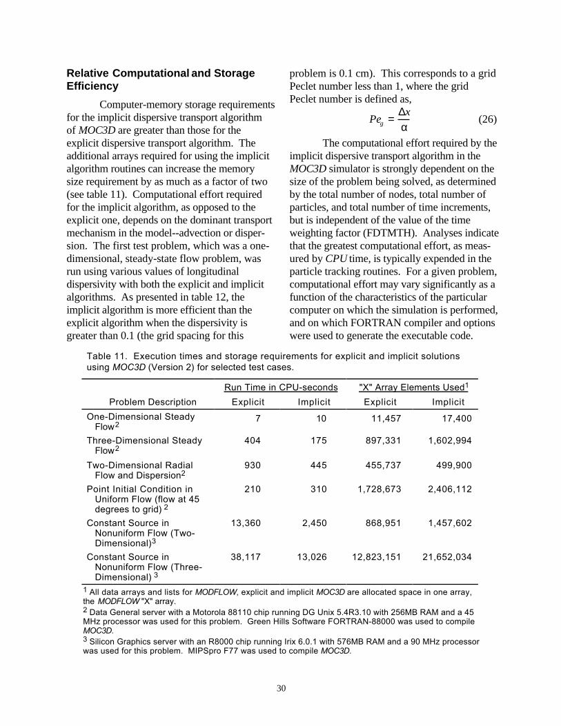
30

Relative Computational and StorageEfficiency

Computer-memory storage requirementsfor the implicit dispersive transport algorithmof MOC3D are greater than those for theexplicit dispersive transport algorithm. Theadditional arrays required for using the implicitalgorithm routines can increase the memorysize requirement by as much as a factor of two(see table 11). Computational effort requiredfor the implicit algorithm, as opposed to theexplicit one, depends on the dominant transportmechanism in the model--advection or disper-sion. The first test problem, which was a one-dimensional, steady-state flow problem, wasrun using various values of longitudinaldispersivity with both the explicit and implicitalgorithms. As presented in table 12, theimplicit algorithm is more efficient than theexplicit algorithm when the dispersivity isgreater than 0.1 (the grid spacing for this

problem is 0.1 cm). This corresponds to a gridPeclet number less than 1, where the gridPeclet number is defined as,

Peg =

∆x

α (26)

The computational effort required by theimplicit dispersive transport algorithm in theMOC3D simulator is strongly dependent on thesize of the problem being solved, as determinedby the total number of nodes, total number ofparticles, and total number of time increments,but is independent of the value of the timeweighting factor (FDTMTH). Analyses indicatethat the greatest computational effort, as meas-ured by CPU time, is typically expended in theparticle tracking routines. For a given problem,computational effort may vary significantly as afunction of the characteristics of the particularcomputer on which the simulation is performed,and on which FORTRAN compiler and optionswere used to generate the executable code.

Table 11. Execution times and storage requirements for explicit and implicit solutionsusing MOC3D (Version 2) for selected test cases.

Run Time in CPU-seconds "X" Array Elements Used1

Problem Description Explicit Implicit Explicit Implicit

One-Dimensional SteadyFlow2

7 10 11,457 17,400

Three-Dimensional SteadyFlow2

404 175 897,331 1,602,994

Two-Dimensional RadialFlow and Dispersion2

930 445 455,737 499,900

Point Initial Condition inUniform Flow (flow at 45degrees to grid) 2

210 310 1,728,673 2,406,112

Constant Source inNonuniform Flow (Two-Dimensional)3

13,360 2,450 868,951 1,457,602

Constant Source inNonuniform Flow (Three-Dimensional) 3

38,117 13,026 12,823,151 21,652,034

1 All data arrays and lists for MODFLOW, explicit and implicit MOC3D are allocated space in one array,the MODFLOW "X" array.2 Data General server with a Motorola 88110 chip running DG Unix 5.4R3.10 with 256MB RAM and a 45MHz processor was used for this problem. Green Hills Software FORTRAN-88000 was used to compileMOC3D.3 Silicon Graphics server with an R8000 chip running Irix 6.0.1 with 576MB RAM and a 90 MHz processorwas used for this problem. MIPSpro F77 was used to compile MOC3D.

31

Table 12. Relative simulation times for explicit and implicit solu-tions using MOC3D (Version 2) for varying values of longitudinaldispersivity for the one-dimensional, steady-state flow problem.

MOC3D

LongitudinalDispersivity (cm)

PecletNumber Explicit Implicit

0.001 100.00 1.0* 2.1

0.010 10.00 1.0 2.1

0.020 5.00 1.0 2.1

0.100 1.00 1.0 2.1

0.200 0.50 1.6 1.8

0.500 0.20 3.7 1.7

1.000 0.10 7.1 1.7

10.000 0.01 67.20 1.6

* A value of 1.0 is equivalent to the base run, which took 6.9 cpuseconds to execute on a Data General server with a Motorola 88110chip running DG Unix 5.4R3.10 with 256 MB RAM and a 45MHzprocessor.

To provide a qualitative indication ofthese relations, we have run all of the sampleproblems described in this report on a varietyof computers. The costs, given as actual runtimes for each problem on selected computersystems, are presented in table 13. The runtimes are measured as CPU time in seconds.As shown in table 13, the running times for agiven problem may vary by more than a factorof ten, depending on which computer wasused. However, for the given test problems,the cost was much more sensitive to the overallsize of the problem. The CPU time on a givencomputer varied by about four orders ofmagnitude between the simplest one-dimensional problem and the most complexthree-dimensional problem. Thus, the modeluser should be aware that simulation cost maybe a serious constraint on the size of problemthat is feasible to simulate.

CONCLUSIONS

The implicit dispersive transportalgorithm presented as an extension to theMOC3D simulator can simulate the transient,

three-dimensional, transport of a solute subjectto decay and retardation. The numericalmethods used to solve the governing equationshave broad general capability and flexibility forapplication to a wide range of hydrogeologicalproblems.

The accuracy and precision of thenumerical results of the implicit dispersivetransport algorithm were tested and evaluatedby comparison to analytical and numericalsolutions for the same set of test problems asreported for the explicit algorithm in MOC3D(Version 1). These evaluation tests indicatethat both the explicit and implicit solutionalgorithms in the MOC3D (Version 2) modelcan successfully and accurately simulate three-dimensional transport and dispersion of asolute in flowing ground water. An advantageof the implicit algorithm is that it has lesscomputational cost for a given accuracy fordispersion-dominated problems. As such, itcomplements the explicit dispersive transportalgorithm, which is more economical foradvection-dominated problems when time steplimitations on the particle transport calculationbecome limiting.

32

Table 13. Comparison of MOC3D (Version 2) simulation times using implicit solver for selectedtest cases on various computer platforms

Run Time in CPU-Seconds

ProblemDescription

Number ofNodes

Numberof

Moves

MaximumNumber ofParticles

SiliconGraphics1

DataGeneralServer2

PC(133 MHz,Pentium)3

MacintoshPowerPC(7300/200)4

One-DimensionalSteady Flow

120 241 360 1.5 10 3 4.5

Three-DimensionalSteady Flow

14,400 27 43,200 16 175 30 83

Two-DimensionalRadial Flow andDispersion

900 282 41,400 33 445 77 158

Point Initial Conditionin Uniform Flow (flowat 45 degrees togrid)

13,824 19 110,729 20 310 40 90

Constant Source inNonuniform Flow(Two-Dimensional)5

12,831 381 57,066 210 2450 420 783

Constant Source inNonuniform Flow(Three-Dimensional)5

192,465 381 855,330 2425 NT NT NT

NT = Not Tested1 Silicon Graphics server with an R8000 chip running Irix 6.0.1 with 576MB RAM and a 90 MHz processor.MIPSpro F77 was used to compile MOC3D.

2 Data General server with a Motorola 88110 chip running DG Unix 5.4R3.10 with 256MB RAM and a 45 MHzprocessor. Green Hills Software FORTRAN-88000 was used to compile MOC3D.

3 IBM-compatible Pentium PC running WindowsNT with 32MB RAM and a 133 MHz processor. Lahey LF90version 4.50e was used to compile MOC3D.

4 Macintosh 7300 with 200 MHz PowerPC 604e processor and 32MB of RAM. MOC3D was compiles usingFortner Research LS FORTRAN Version 1.1 for Power Mac.

5 CELDIS = 0.5

REFERENCES

Axelsson, Owe, 1994, Iterative Solution Methods: NewYork, Cambridge University Press, 654 p.

Aziz, Khalid, and Settari, Antonin, 1979, Petroleumreservoir simulation: London, England, AppliedScience, 476 p.

Burnett, R.D., and Frind, E.O., 1987, Simulation ofcontaminant transport in three dimensions, 2.Dimensionality effects: Water ResourcesResearch, v. 23, no. 4, p. 695-705.

Dupont, R.P., Kendall, Todd, and Rachford, Henry,1968, An approximate factorization procedure forsolving self-adjoint elliptic difference equations:SIAM Journal of Numerical Analysis, v. 53, p.559-573

Garder, A.O., Peaceman, D.W., Pozzi, A.L., 1964,Numerical calculation of multidimensionalmiscible displacement by the method ofcharacteristics: Soc. Petroleum Eng. Jour., v. 4,no. 1, p. 26-36.

33

Goode, D.J., and Konikow, L.F., 1989, Modification ofa method-of-characteristics solute-transport modelto incorporate decay and equilibrium-controlledsorption or ion exchange: U.S. GeologicalSurvey Water-Resources Investigations Report89-4030, 65 p.

Harbaugh, A.W., and McDonald, M.G., 1996a, User'sdocumentation for MODFLOW-96, an update tothe U.S. Geological Survey modular finite-difference ground-water flow model: U.S.Geological Survey Open-File Report 96-485, 56p.

Harbaugh, A.W., and McDonald, M.G., 1996b,Programmer's documentation for MODFLOW-96, an update to the U.S. Geological Surveymodular finite-difference ground-water flowmodel: U.S. Geological Survey Open-FileReport 96-486, 220 p.

Hsieh, P.A., 1986, A new formula for the analyticalsolution of the radial dispersion problem: WaterResources Research, v. 22, no. 11, p. 1597-1605.

Kipp, K.L., 1987, HST3D: A computer code forsimulation of heat and solute transport in three-dimensional ground-water flow: U.S. GeologicalSurvey Water-Resources Investigations Report86-4095, 517 p.

Konikow, L.F., and Bredehoeft, J.D., 1978, Computermodel of two-dimensional solute transport anddispersion in ground water: U.S. GeologicalSurvey Techniques of Water-ResourcesInvestigations, Book 7, Chapter C2, 90 p.

Konikow, L.F., Goode, D.J., and Hornberger, G.Z.,1996, A three-dimensional method-of-characteristics solute-transport model (MOC3D):

U.S. Geological Survey Water-ResourcesInvestigations Report 96-4267, 87 p.

McDonald, M.G., and Harbaugh, A.W., 1988, Amodular three-dimensional finite-differenceground-water flow model: U.S. GeologicalSurvey Techniques of Water-ResourcesInvestigations, Book 6, Chapter A1, 586 p.

Meijerink, J.A., and Van der Vorst, H.A., 1977, Aniterative solution method for linear systems ofwhich the coefficient matrix is a symmetric M-matrix: Mathematics of Computation, v. 31, no.137, p. 148-162.

Meijerink, J.A., and Van der Vorst, H.A., 1981,Guidelines for the usage of incompletedecompositions in solving sets of linearequations as they occur in practical problems:Journal of Computational Physics, v. 44, p.134-155.

Price, H.S., and Coats, K.H., 1974, Direct methods inreservoir simulation: Transactions of the Societyof Petroleum Engineers of the American Instituteof Mining, Metallurgical, and PetroleumEngineers, v. 257, p. 295-308.

Stoer, J., and Bulirsch, R., 1991, Introduction toNumerical Analysis: 2nd ed., Springer-Verlag,New York, 660 p.

Wexler, E.J., 1992, Analytical solutions for one-, two-,and three-dimensional solute transport in ground-water systems with uniform flow: U.S.Geological Survey Techniques of Water-Resources Investigations, Book 3, Chapter B7,190 p.

Yanenko, N.N., 1971, The Method of Fractional Steps:Springer-Verlag, New York, 160 p.

34

APPENDIX A: DATA INPUT INSTRUCTIONS FOR MOC3D (Version 2)

This Appendix includes a complete set of instructions for preparing a data set for theMOC3D model. Major changes that have been implemented since the release of Version 1 areshaded to highlight the new instructions.

MODFLOW Name File

Transport simulation is activated by including a record in the MODFLOW name file usingthe file type (Ftype) “CONC” to link to the transport name file. The transport name file specifiesthe files to be used when simulating solute transport in conjunction with a simulation of ground-water flow using MODFLOW. The transport name file works in the same way as the MODFLOWname file.

MODFLOW Source and Sink Packages

Except for recharge, concentrations associated with fluid sources (C') are read as auxiliaryparameters in the MODFLOW source package. The source concentration is read from a newcolumn appended to the end of each line of the data file describing a fluid sink/source (seedocumentation for revised MODFLOW model; Harbaugh and McDonald, 1996a and 1996b). Forexample, concentrations associated with well nodes should be appended to the line in the WELPackage where the well’s location and pumping rate are defined. These concentrations will be readif the auxiliary parameter “CONCENTRATION” (or “CONC”) appears on the first line of the wellinput data file. The concentration in recharge is defined separately, as described in followingsection “Source Concentration in Recharge File.”

To simulate solute transport the MODFLOW option enabling storage of cell-by-cell flowrates for each fluid source or sink is required in all fluid packages except recharge. The key word“CBCALLOCATE” (or “CBC”) must appear on the first line of each input data file for a fluidpackage (see Harbaugh and McDonald, 1996a and 1996b).

MOC3D Input Data Files

All input variables are read using free formats, except as specifically indicated. In freeformat, variables are separated by one or more spaces or by a comma and optionally one or morespaces. Blank spaces are not read as zeros.

35

MOC3D Transport Name File (CONC)

FOR EACH SIMULATION:

1. Data: FTYPE NUNIT FNAME

The name file consists of records defining the names and units numbers of the files. Each“record” consists of a separate line of data. There must be a record for the listing file and for themain MOC3D input file.

The listing (or output) file (“CLST”) must be the first record. The other files may be in anyorder. Each record can be no more than 79 characters.

FTYPE The file type, which may be one of the following character strings:

CLST MOC3D listing file (separate from the MODFLOW listing file) [required].

MOC or MOCIMP Main MOC3D input data file [required]. Specifying MOCindicates dispersion calculations will be explicit (as described by Konikowand others, 1996) and specifying MOCIMP indicates dispersioncalculations will be implicit (as described in this report).

CRCH Concentrations in recharge [optional].

CNCA Separate output file containing concentration data in ASCII (text-only) format.Frequency and format of printing controlled by NPNTCL and ICONFM[optional]. If concentrations are written to a separate output file, they willnot be written to the main output file.

CNCB Separate output file containing concentration data in binary format [optional].

VELA Separate output file with velocity data in ASCII format. Frequency and formatof printing controlled by NPNTVL and IVELFM [optional].

VELB Separate output file with velocity data in binary format [optional].

PRTA Separate output file with particle locations printed in ASCII format. Frequencyand format of printing controlled by NPNTPL [optional].

PRTB Separate output file with particle locations printed in binary format [optional].

OBS Observation wells input file [optional].

DATA For formatted files such as those required by the OBS package and for arraydata separate from the main MOC3D input data file [optional].

DATA(BINARY) For formatted input/output files [optional].

NUNIT The FORTRAN unit number used to read from and write to files. Any legal unitnumber other than 97, 98, and 99 (which are reserved by MODFLOW) can beused provided that it is not previously specified in the MODFLOW name file.

FNAME The name of the file.

36

Main MOC3D Package Input (MOC or MOCIMP)

Input for the method-of-characteristics (MOC3D) solute-transport package is read from theunit specified in the transport name file. The input consists of up to 19 separate records or datasets, as described in detail below. These data are used to specify information about the transportsubgrid, physical and chemical transport parameters, numerical solution variables, and outputformats. Output file controls for the MOC3D package are specified in the transport name file,described previously. Compared to the original version of MOC3D, Version 2 includes oneadditional data set, which is used only if the implicit solver is selected. This data set is placedbetween the original data sets 7 and 8, and hence has been labeled as data set 7.1.

FOR EACH SIMULATION:

1. Data: HEDMOC A two-line character-string title describing thesimulation (80 text characters per line).

2. Data: HEDMOC (continued)

3. Data: ISLAY1 ISLAY2 ISROW1 ISROW2 ISCOL1 ISCOL2

ISLAY1 Number of first (uppermost) layer for transport.

ISLAY2 Last layer for transport.

ISROW1 First row for transport.

ISROW2 Last row for transport.

ISCOL1 First column for transport.

ISCOL2 Last column for transport.

Notes:

Transport may be simulated within a subgrid, which is a “window” within the primaryMODFLOW grid used to simulate flow. Within the subgrid, the row and column spacing must beuniform, but thickness can vary from cell to cell and layer to layer. However, as discussed in thesection reviewing MOC3D assumptions, the range in thickness values (or product of thickness andporosity) should be as small as possible.

4. Data: NODISP DECAY DIFFUS

NODISP Flag for no dispersion (set NODISP=1 if no dispersion in problem; this will reducestorage allocation).

DECAY First-order decay rate [1/T] (DECAY=0.0 indicates no decay occurs).

DIFFUS Effective molecular diffusion coefficient [L2/T].

Notes:

The decay rate (λ) is related to the half life (t1/2) of a constituent by λ = (ln 2)/t1/2.

The effective molecular diffusion coefficient (Dm) includes the effect of tortuosity.

37

5. Data: NPMAX NPTPND

NPMAX Maximum number of particles available for particle tracking of advective transportin MOC3D. If set to zero, the model will calculate NPMAX according to thefollowing equation:

NPMAX = 2× NPTPND× NSROW× NSCOL× NSLAY.

NPTPND Initial number of particles per cell in transport simulation (that is, at t = 0.0). Validoptions for default geometry of particle placement include 1, 2, 3, or 4 for one-dimensional transport simulation; 1, 4, 9, or 16 for two-dimensional transportsimulation; and 1, 8, or 27 for three-dimensional transport simulation. The usercan also customize initial placement of particles by specifying NPTPND as anegative number, in which case the minus sign is recognized as a flag toindicate custom placement is desired. In this case, the user must input localparticle coordinates as described below.

IF NPTPND IS NEGATIVE IN SIGN:

6. Data: PNEWL PNEWR PNEWC

PNEWL Relative position in the layer (z) direction for initial placement of particle within anyfinite-difference cell.

PNEWR Relative position in the row (y) direction for initial placement of particle.

PNEWC Relative position in the column (x) direction for initial placement of particle.

Notes:

The three new (or initial) particle coordinates are entered sequentially for each of theNPTPND particles. Each line contains the three relative local coordinates for the new particles, inorder of layer, row, and column. There must be NPTPND lines of data, one for each particle. Thelocal coordinate system range is from -0.5 to 0.5, and represents the relative distance within the cellabout the node location at the center of the cell, so that the node is located at 0.0 in each direction.

FOR EACH SIMULATION:

7. Data: CELDIS FZERO INTRPL

CELDIS Maximum fraction of cell dimension that particle may move in one step (typically,0.5 ≤ CELDIS ≤1.0 ).

FZERO If the fraction of active cells having no particles exceeds FZERO, the program willautomatically regenerate an initial particle distribution before continuing the simulation(typically, 0.01 ≤ FZERO ≤ 0.05 ).

INTRPL Flag for interpolation scheme used to estimate velocity of particles. The default(INTRPL=1) will use a linear interpolation routine; if INTRPL=2, a scheme will beimplemented that uses bilinear interpolation in the row and column (j and i)directions only (linear interpolation will still be applied in the k, or layer, direction).(See section “Discussion—Choosing appropriate interpolation scheme.”)

38

FOR EACH SIMULATION (only if MOCIMP is specified in Transport Name File):

7.1 Data: FDTMTH NCXIT IDIREC EPSSLV MAXIT

FDTMTH Weighting factor for temporal differencing of dispersion equation (0.0 ≤ FDTMTH ≤1.0). We suggest using either a value of FDTMTH = 0.5, a centered-in-time (orCrank-Nicolson) approximation, or FDTMTH = 1.0, a backward-in-time (or fullyimplicit) approximation. [Default value = 1]

NCXIT Number of iterations for the explicitly-lagged cross-dispersive flux terms (NCXIT ≥ 1).We suggest that the user initially specify a value of 2, but if the solution exhibitssignificant areas of negative concentrations, then the value of NCXIT should beincreased to require more iterations, which typically will reduce the extent andmagnitude of negative concentrations (at the cost of increased computational time).[Default value = 2]

IDIREC Direction index for permutation of the red-black node renumbering scheme. The orderis as follows: 1: x,y,z; 2: x,z,y; 3: y,x,z; 4: y,z,x; 5: z,x,y; and 6: z,y,x. The firstdirection index is advanced most rapidly and the last direction index is advancedleast rapidly. In some cases, there can be a significant variation in the number ofiterations needed to achieve convergence, depending on the order of the directionsfor the red-black renumbering. We suggest that the user initially specify IDIREC =1. If this leads to a relatively large number of iterations (more than 10), then the usershould experiment with alternate choices to determine the one requiring the fewestnumber of iterations for their particular problem. [Default value = 1]

EPSSLV Tolerance on the relative residual for the conjugate-gradient solution of the matrix of thedifference equations. We suggest that the user initially specify EPSSLV ≤ 10-5. Anadequately small value of EPSSLV has the property that a smaller value does notchange the numerical solution within the number of significant digtits desired by theuser. In the single-precision code implemented here, EPSSLV should not be lessthan 10-7. [Default value = 10-5]

MAXIT Maximum number of iterations allowed for the iterative solution to the differernceequations for dispersive transport. In most cases, MAXIT = 100 is satisfactory.[Default value = 100]

Notes:

Entering a zero or out-of-range value for any of these five variables will cause the code touse the indicated default value.

39

FOR EACH SIMULATION:

8. Data: NPNTCL ICONFM NPNTVL IVELFM NPNTDL IDSPFM NPNTPL

NPNTCL Flag for frequency of printing concentration data. If NPNTCL=-2, concentration datawill be printed at the end of every stress period; if NPNTCL=-1, data will beprinted at the end of every flow time step; if NPNTCL=0, data will be printed at theend of the simulation; if NPNTCL=N>0, data will be printed every Nth particlemoves, and at the end of the simulation. Initial concentrations are always printed.Solute budget and mass balance information are only printed every timeconcentration data are saved.

ICONFM Flag for output format control for printing concentration data. If concentration data arewritten to main output file (file type CNCA is not used), ICONFM represents a codeindicating the format style (table 14, also see Harbaugh and McDonald, 1996a, p.19). If concentration data are written to a separate output file (file type CNCAexists), specifying ICONFM ≥ 0 will indicate that concentration data are to bewritten as a matrix of values for each layer of the subgrid, whereas specifyingICONFM < 0 will indicate that concentration data are to be written as a table ofvalues having one row for each node in the subgrid and four columns (x, y, z, andconcentration), where x, y, and z are the actual nodal coordinates in the length unitsof the model simulation. Note that we follow the MODFLOW convention in that yincreases from top to bottom row, and z increases from top layer to bottom layer.Also note that the x and y values are given with respect to the entire MODFLOWgrid, but the z location is calculated only for vertical distances within the layers ofthe transport subgrid. If data are written in matrix style, one header line precedesand identifies the data for each layer. If data are written as a table of values, oneheader line is written each time that concentration data are saved.

NPNTVL Flag for printing velocity data. If NPNTVL=-1, velocity data will be printed at the endof every stress period; if NPNTVL=0, data will be printed at the end of thesimulation; if NPNTVL=N>0, data will be printed every Nth flow time steps, andat the end of the simulation.

IVELFM Specification for format of velocity data, if being printed in main output file (see table14).

NPNTDL Flag for printing dispersion equation coefficients that include cell dimension factors(see section “Program Segments”). If NPNTDL=-2, coefficients will be printed atthe end of every stress period; if NPNTDL=-1, coefficients will be printed at theend of the simulation; if NPNTDL=0, coefficients will not be printed; ifNPNTDL=N>0, coefficients will be printed every Nth flow time step.

IDSPFM Specification for format of dispersion equation coefficients (see table 14).

NPNTPL Flag for printing particle locations in a separate output file (only used if file types“PRTA” or “PRTB” appear in the MOC3D name file). If neither “PRTA” or“PRTB” is entered in the name file, NPNTPL will be read but ignored (so you mustalways have some value specified here). If either “PRTA” or “PRTB” is entered inthe name file, initial particle locations will be printed to the separate file first,

40

followed by particle data at intervals determined by the value of NPNTPL. IfNPNTPL=-2, particle data will be printed at the end of every stress period; ifNPNTPL=-1, data will be printed at the end of every flow time step; ifNPNTPL=0, data will be printed at the end of the simulation; if NPNTPL=N>0,data will be printed every Nth particle moves, and at the end of the simulation.

Table 14. Formats associated with MOC3D print flags. (Positive values for wrap format;negative values for strip format. Also see Harbaugh and McDonald, 1996a, p. 19.)

Print flag Format Print flag Format Print flag Format

0 10G11.4 7 20F5.0 14 10F6.1

1 11G10.3 8 20F5.1 15 10F6.2

2 9G13.6 9 20F5.2 16 10F6.3

3 15F7.1 10 20F5.3 17 10F6.4

4 15F7.2 11 20F5.4 18 10F6.5

5 15F7.3 12 10G11.4

6 15F7.4 13 10F6.0

FOR EACH SIMULATION:

9. Data: CNOFLO Concentration associated with inactive cells of subgrid (used foroutput purposes only).

FOR EACH LAYER OF THE TRANSPORT SUBGRID:

10. Data: CINT(NSCOL,NSROW) Initial concentration. Module: U2DREL*

FOR EACH SIMULATION, ONLY IF TRANSPORT SUBGRID DIMENSIONS ARESMALLER THAN FLOW GRID DIMENSIONS:

11. Data: CINFL(ICINFL) ′ C to be associated with fluid inflow across theboundary of the subgrid.

Module: U1DREL*

Notes:The model assumes that the concentration outside of the subgrid is the same within each

layer, so only one value of CINFL is specified for each layer within and adjacent to the subgrid. Thatis, the size of the array (ICINFL) is determined by the position of the subgrid with respect to theentire (primary) MODFLOW grid. If the transport subgrid has the same dimensions as the flow grid,

* Module is a standard MODFLOW input/output module.

41

this parameter should not be included in the input data set. If the subgrid and flow grid have thesame number of layers, but the subgrid has fewer rows or fewer columns, ICINFL=NSLAY. Valuesare also required if there is a flow layer above the subgrid and/or below the subgrid. The order ofinput is: ′ C for first (uppermost) transport layer (if required); ′ C for each successive (deeper)transport layer (if required); ′ C for layer above subgrid (if required); and ′ C for layer belowsubgrid (if required).

FOR EACH SIMULATION:

12. Data: NZONES Number of zone codes among fixed-head nodes in transport subgrid.

IF NZONES > 0:

Data: IZONE ZONCON

IZONE Value identifying a particular zone.ZONCON Source concentration associated with nodes in the zone defined by IZONE above.

Notes:Zones are defined within the IBOUND array in the BAS Package of MODFLOW by

specifying unique negative values for fixed-head nodes to be associated with separate fluid sourceconcentrations. Each zone is defined by a unique value of IZONE and a concentration associatedwith it (ZONCON). There must be NZONES lines of data, one for each zone. Note that values ofIZONE in this list must be negative for consistency with the definitions of fixed-head nodes in theIBOUND array in the BAS Package. If a negative value of IBOUND is defined in the BAS packagebut is not assigned a concentration value here, MOC3D will assume that the source concentrationsassociated with those nodes equal 0.0.

FOR EACH LAYER OF THE TRANSPORT SUBGRID:

13. Data: IGENPT(NSCOL,NSROW) Flag to treat fluid sources and sinks aseither “strong” or “weak.”

Module: U2DINT*

Notes:Where fluid source is “strong,” new particles are added to replace old particles as they are

advected out of that cell. Where a fluid sink is “strong,” particles are removed after they enter thatcell and their effect accounted for. Where sources or sinks are weak, particles are neither added norremoved, and the source/sink effects are incorporated directly into appropriate changes in particlepositions and concentrations. If IGENPT=0, the node will be considered a weak source or sink; ifIGENPT=1, it will be a strong source or sink. See section on “Special Problems” and discussion byKonikow and Bredehoeft (1978).

* Module is a standard MODFLOW input/output module.

42

IF NODISP ≠ 1 (If dispersion is included in simulation):

14. Data: ALONG(NSLAY) Longitudinal dispersivity. Module: U1DREL*

15. Data: ATRANH(NSLAY) Horizontal transverse dispersivity. Module: U1DREL*

16. Data: ATRANV(NSLAY) Vertical transverse dispersivity. Module: U1DREL*

FOR EACH SIMULATION:

17. Data: RF(NSLAY) Retardation factor (RF=1 indicates no retardation). Module: U1DREL*

Notes:If RF=0.0 in input, the code automatically resets it as RF=1.0 to indicate no retardation.

FOR EACH LAYER OF TRANSPORT SUBGRID:

18a. Data: THCK(NSCOL,NSROW) Cell thickness. Module: U2DREL*

18b. Data: POR(NSCOL,NSROW) Cell porosity. Module: U2DREL*

Notes:The thickness and porosity are input as separate arrays for each layer of the transport

subgrid. The sequence used in data set 18 is to first define the thickness of the first layer of thetransport subgrid, and then define the porosity of that same layer. Next, that sequence is repeated forall succeeding layers. The product of thickness and porosity should not be allowed to vary greatlyamong cells in the transport subgrid.

* Module is a standard MODFLOW input/output module.

43

Source Concentration in Recharge File (CRCH)

Concentrations in recharge, if the recharge package is used, are read from a separate unitspecified in the MOC3D name file. This is defined using the file type (Ftype) “CRCH.”

FOR EACH STRESS PERIOD, IF RECHARGE PACKAGE USED:

1. Data: INCRCH Flag to reuse or read new recharge concentrations.

Notes:Read new recharge concentrations if INCRCH ≥ 0. Reuse recharge concentrations from the

last stress period if INCRCH < 0.

2. Data: CRECH(NSCOL,NSROW) Source concentration associated with fluidentering the aquifer in recharge.

Module: U2DREL*

Observation Well File (OBS)

Nodes of the transport subgrid can be designated as “observation wells.” At each suchnode, the time, head, and concentration after each move increment will be written to a separateoutput file to facilitate graphical postprocessing of the calculated data. The input file for specifyingobservation wells is read if the file type (Ftype) “OBS” is included in the MOC3D name file.

FOR EACH SIMULATION, IF OBS PACKAGE USED:

1. Data: NUMOBS IOBSFL

NUMOBS Number of observation wells.

IOBSFL If IOBSFL = 0, well data are saved in NUMOBS separate files. If IOBSFL>0, allobservation well data will be written to one file, and the file name and unitnumber used for this file will be that of the first observation well in the list.

FOR EACH OBSERVATION WELL:

2. Data: LAYER ROW COLUMN UNIT

LAYER Layer of observation well node.ROW Row of observation well node.COLUMN Column of observation well node.UNIT Unit number for output file.

Notes:If NUMOBS>1 and IOBSFL = 0, you must specify a unique unit number for each observa-

tion well and match those unit numbers to DATA file types and file names in the MOC3D name file.If IOBSFL>0, you must specify a unique unit number for the first observation well and match thatunit number to a DATA file type and file name in the MOC3D name file. * Module is a standard MODFLOW input/output module.

44

APPENDIX B: ANNOTATED INPUT DATA SET FOR EXAMPLEPROBLEM

This example input data set is the one used to generate the solution for the base case in theone-dimensional steady-state flow problem. Parameter values are indicated in table 6 and selectedresults are shown in figures 4 and 6. Several of the following data files (finite.nam, finite.bas,finite.bcf, and finite.sip) are those required for MODFLOW-96, and their formats are describedby Harbaugh and McDonald (1996a).

In the data files shown below, the right side of some data lines includes a semi-colonfollowed by text that describes the parameters for which values are given. These comments(including the semi-colon) are not read by the program because in free format the code will onlyread the proper number of variables and ignore any subsequent information on that line. This styleof commenting data files is optional, but users may find it helpful when preparing their own datafiles.

Information pertaining specifically to the implicit solution is highlighted by shading.

Following (enclosed in a border) are the contents of the MODFLOW name file for thesample problem; explanations are noted outside of border:

File name: finite.nam

list 16 finite.lst ← Designates main output file for MODFLOW

bas 95 finite.bas ← Basic input data for MODFLOW

bcf 11 finite.bcf ← Block-centered flow package

sip 19 finite.sip ← Input for numerical solution of flow equation

conc 33 fint_moc.nam ← Transport name file (turns transport “on”)

↑ ↑ ↑ 1 2 3

1 Ftype (that is, the type of file)2 Unit number3 File name (name chosen to reflect contents of file)

45

Following (enclosed in a border) are the contents of the basic package input data file for theMODFLOW simulation of the sample problem; explanations are noted outside of border:

File name: finite.bas

Finite: Compare to Wexler program and MOC3D BAS Input ← 1

NLAY NROW NCOL NPER ITMUNI ← 1

1 1 122 1 1 ← 2

FREE CHTOCH ← 3

0 1 ; IAPART,ISTRT ← 4

95 1(25I3) 3 ; IBOUND ← 5

-1 1 1 1 1 1 1 1 1 1 1 1 1 1 1 1 1 1 1 1 1 1 1 1 1 ← 5

1 1 1 1 1 1 1 1 1 1 1 1 1 1 1 1 1 1 1 1 1 1 1 1 1 ← 5

1 1 1 1 1 1 1 1 1 1 1 1 1 1 1 1 1 1 1 1 1 1 1 1 1 ← 5

1 1 1 1 1 1 1 1 1 1 1 1 1 1 1 1 1 1 1 1 1 1 1 1 1 ← 5

1 1 1 1 1 1 1 1 1 1 1 1 1 1 1 1 1 1 1 1 1 -2 ← 5

0.00 ; HNOFLO ← 6

95 1.0(122F6.0) 1 ; HEAD ← 7

12.1 ← 7

120.0 1 1. ; PERLEN,NSTP,TSMULT ← 8

1 Two header lines of comments. For convenience and clarity, the second line is used to label names ofparameters on subsequent line of file.

2 Flow grid dimensions, number of periods, and time units.3 Options line (new in MODFLOW-96)4 Flags for buffer array and drawdown calculations.5 IBOUND identifiers (first line) and array6 Head value assigned to inactive cells7 Initial head information8 MODFLOW time-step information

Following (enclosed in a border) are the contents of the block-centered flow package inputdata file; explanations are noted outside of border:

File name: finite.bcf

1 0 0.0 0 0.0 0 0 ; ISS,flags BCF Input ← 1

0 ; LAYCON ← 2

0 1.0 ; TRPY ← 3

0 0.1 ; DELR ← 4

0 0.1 ; DELC ← 4

0 0.01 ; TRAN

1 Flag for steady-state flow, flag for cell-by-cell flow terms, five flags related to wetting2 Layer type3 Anisotropy factor4 Grid spacing information

46

Following (enclosed in a border) are the contents of the strongly implicit procedure packageinput data file; explanations are noted outside of border:

File name: finite.sip

500 5 ; MXITER,NPARM SIP Input ← 1

1. 0.0000001 0 0.001 0 ; ACCL,HCLOSE,IPCALC,WSEED,IPRSIP ← 2

1 Maximum iterations, number of iteration parameters2 Acceleration parameter, head change criterion, flag for seed, seed, printout interval for SIP

Following (enclosed in a border) are the contents of the MOC3D name file for the sampleproblem; explanations are noted outside of border:

File name: fint_moc.nam

clst 94 finite.out ← Designates main output file for MOC3D

mocimp 96 fint_imp.moc ← Main input data file for MOC3D

obs 44 finite.obs ← Input data file for observation wells

data 45 finite.oba ← Output file for observation well data

cnca 22 finite.cna ← Separate output file for concentration data (ASCII)

↑ ↑ ↑ 1 2 3

1 Ftype2 Unit number3 File name

47

Following (enclosed in a border) are the contents of the main input data file for the MOC3Dsimulation for the sample problem; selected explanations are noted outside of border:

File name: finite_imp.mocOne-dimensional, Steady Flow, No Decay, Low Dispersion: MOC3D (Implicit) ← 1 ISLAY1 ISLAY2 ISROW1 ISROW2 ISCOL1 ISCOL2 ← 1 1 1 1 1 2 121 ← 2 0 0.00 0.0 ; NODISP, DECAY, DIFFUS ← 3 0 3 ; NPMAX, NPTPND ← 4 0.5 0.05 2 ; CELDIS, FZERO, INTRPL ← 4 0.5 2 1 1.e-05 100 ; FDTMTH,NXCIT,IDIR,EPSSLV,MAXIT ← 5 0 -1 0 0 0 0 0 ; NPNTCL, ICONFM, NPNTVL, IVELFM, NPNTDL, IDSPFM, NPRTPL ← 6 0.0 ; CNOFLO ← 7 0 0.0 (122F3.0) ; initial concentration 0 1. ; C' inflow 2 ; NZONES to follow ← 8 -1 1.0 ; IZONE, ZONCON ← 8 -2 0.0 ; IZONE, ZONCON ← 8 0 0 ; IGENPT ← 9 0 0.1 ; longitudinal disp. 0 0.1 ; transverse disp. horiz. 0 0.1 ; transverse disp. vert. 0 1.0 ; retardation factor 0 1.0 ; thickness 0 0.1 ; porosity

1 Two header lines of comments. For convenience and clarity, the second line is used to label names ofparameters on subsequent line of file.

2 Indices for transport subgrid3 Flag for no dispersion, decay rate, diffusion coefficient4 Particle information for advective transport5 Information to control implicit dispersion calculations6 Print flags7 Value of concentration associated with inactive cells8 Concentrations associated with fixed-head nodes (fixed head nodes are defined in the IBOUND array in the

MODFLOW BAS package)9 Flag for “strong” sources or sinks

Following (enclosed in a border) are the contents of the observation well input data file forthe sample problem; explanations are noted outside of border:

File name: finite.obs

3 1 ;NUMOBS IOBSFL Observation well data ← 1 1 1 2 45 ;layer, row, column, unit number ← 2 1 1 42 ;layer, row, column ← 2 1 1 112 ;layer, row, column ← 2

1 Number of observation wells, flag to print to one file or separate files2 Node location and unit number for output file (linked to the Ftype DATA in MOC3D name file)

48

APPENDIX C: SELECTED OUTPUT FOR EXAMPLE PROBLEM

This example output was generated from the input data sets listed in Appendix B for thebase case of the one-dimensional steady-state flow problem. We do not include the mainMODFLOW listing (output) file. The line spacing and font sizes of the output files have beenmodified in places to enhance the clarity of reproduction in this report. Some repetitive lines ofoutput have been deleted where indicated by an ellipsis (. . . ). Output related specifically to theimplicit solution is highlighted by shading.

Some brief annotations were added to this sample output listing to help the readerunderstand the purpose of various sections of output. These annotations are written in bold italics.

Following are the contents of the MOC3D main output file (finite.out) for the sampleproblem.

U.S. GEOLOGICAL SURVEY METHOD-OF-CHARACTERISTICS SOLUTE-TRANSPORT MODEL MOC3D (Version 2.0) 11/16/98

MOC BASIC INPUT READ FROM UNIT LISTING FILE: finite.out UNIT 94

OPENING fint_imp.moc FILE TYPE: MOCIMP UNIT 96

OPENING finite.obs FILE TYPE: OBS UNIT 44

OPENING finite.oba FILE TYPE: DATA UNIT 45

OPENING finite.cna FILE TYPE: CNCA UNIT 22

MOC BASIC INPUT READ FROM UNIT 96

2 TITLE LINES: One-dimensional, Steady Flow, No Decay, Low Dispersion: MOC3D (Implicit) ISLAY1 ISLAY2 ISROW1 ISROW2 ISCOL1 ISCOL2

PROBLEM DESCRIPTORS, INCLUDING GRID CHARACTERISTICS AND PARTICLE INFORMATION: MAPPING OF SOLUTE TRANSPORT SUBGRID IN FLOW GRID: FIRST LAYER FOR SOLUTE TRANSPORT = 1 LAST LAYER FOR SOLUTE TRANSPORT = 1 FIRST ROW FOR SOLUTE TRANSPORT = 1 LAST ROW FOR SOLUTE TRANSPORT = 1 FIRST COLUMN FOR SOLUTE TRANSPORT= 2 LAST COLUMN FOR SOLUTE TRANSPORT = 121

UNIFORM DELCOL AND DELROW IN SUBGRID FOR SOLUTE TRANSPORT

NO. OF LAYERS = 1 NO. OF ROWS = 1 NO. OF COLUMNS = 120 NO SOLUTE DECAY NO MOLECULAR DIFFUSION MAXIMUM NUMBER OF PARTICLES (NPMAX) = 720 13669 ELEMENTS IN X ARRAY ARE USED BY MOC 12 ELEMENTS IN X ARRAY ARE USED BY OBS

FILE INFORMATION

49

NUMBER OF PARTICLES INITIALLY IN EACH ACTIVE CELL (NPTPND) = 3 PARTICLE MAP ("o" indicates particle location; shown as fractions of cell distances relative to node location):

o------o------o

-1/3 0 1/3

INITIAL RELATIVE PARTICLE COORDINATES 1 0.00000 0.00000 -0.33333 2 0.00000 0.00000 0.00000 3 0.00000 0.00000 0.33333

CELDIS= 0.500 FZERO = 0.050

INTRPL= 2; BILINEAR INTERPOLATION SCHEME

NUMERICAL PARAMETERS FOR IMPLICIT SOLVER: FDTMTH = 0.50 NCXIT = 2 IDIREC = 1 EPSSLV = 1.0000E-05 MAXIT = 100

NPNTCL= 0: CONCENTRATIONS WILL BE WRITTEN AT THE END OF THE SIMULATIONMODFLOW FORMAT SPECIFIER FOR CONCENTRATION DATA: ICONFM= -1

NPNTVL= 0: VELOCITIES WILL BE WRITTEN AT THE END OF THE SIMULATIONMODFLOW FORMAT SPECIFIER FOR VELOCITY DATA: IVELFM= 0

NPNTDL= 0: DISP. COEFFICIENTS WILL NOT BE WRITTEN

NPNTPL= 0: PARTICLE LOCATIONS WILL NOT BE WRITTEN

CONCENTRATION WILL BE SET TO 0.00000E+00 AT ALL NO-FLOW NODES (IBOUND=0).

INITIAL CONCENTRATION = 0.0000000E+00 FOR LAYER 1

VALUES OF C' REQUIRED FOR SUBGRID BOUNDARY ARRAY = 1ONE FOR EACH LAYER IN TRANSPORT SUBGRID

ORDER OF C' VALUES: FIRST LAYER IN SUBGRID, EACH SUBSEQUENT LAYER,LAYER ABOVE SUBGRID, LAYER BELOW SUBGRID:

SUBGRID BOUNDARY ARRAY = 1.000000

NUMBER OF ZONES FOR CONCENTRATIONS AT FIXED HEAD CELLS = 2

ZONE FLAG = -1 INFLOW CONCENTRATION = 1.0000E+00 ZONE FLAG = -2 INFLOW CONCENTRATION = 0.0000E+00

SINK-SOURCE FLAG = 0 FOR LAYER 1

LONGITUDNL. DISPERSIVITY = 0.1000000

HORIZ. TRANSVERSE DISP. = 0.1000000

VERT. TRANSVERSE DISP. = 0.1000000

OUTPUT

CONTROL

INITIAL AND

BOUNDARY

CONDITIONS

FOR SOLUTE

50

RETARDATION FACTOR = 1.000000

INITIAL THICKNESS = 1.000000 FOR LAYER 1

INITIAL POROSITY = 0.1000000 FOR LAYER 1

COORDINATES FOR 3 OBSERVATION WELLS:

WELL # LAYER ROW COLUMN UNIT 1 1 1 2 45 2 1 1 42 45 3 1 1 112 45ALL OBSERVATION WELL DATA WILL BE WRITTEN ON UNIT 45

CONCENTRATION DATA WILL BE SAVED ON UNIT 22 IN X,Y,Z,CONC FORMAT

TOTAL NUMBER OF PARTICLES GENERATED = 360 TOTAL NUMBER OF ACTIVE NODES (NACTIV) = 120 MAX. NUMBER OF CELLS THAT CAN BE VOID OF PARTICLES (NZCRIT) = 6 (IF NZCRIT EXCEEDED, PARTICLES ARE REGENERATED)

CALCULATED VELOCITIES (INCLUDING EFFECTS OF RETARDATION, IF PRESENT):

EFFECTIVE MEAN SOLUTE VELOCITIES IN COLUMN DIRECTION AT NODES

1VELOCITY (COL) IN LAYER 1 AT END OF TIME STEP 1 IN STRESS PERIOD 1 -----------------------------------------------------------------------

1 2 3 4 5 6 7 ...... ....................................................................................................... ... 1 0.1000 0.1000 0.1000 0.1000 0.1000 0.1000 0.1000 ...

...

EFFECTIVE MEAN SOLUTE VELOCITIES IN ROW DIRECTION AT NODES

1 VELOCITY (ROW) IN LAYER 1 AT END OF TIME STEP 1 IN STRESS PERIOD 1 -----------------------------------------------------------------------

1 2 3 4 5 6 7 8 9 ...... ........................................................................................................ ... 1 0.000E+00 0.000E+00 0.000E+00 0.000E+00 0.000E+00 0.000E+00 0.000E+00 0.000E+00 0.000E+00 ...

...

EFFECTIVE MEAN SOLUTE VELOCITIES IN LAYER DIRECTION AT NODES

1 VELOCITY (LAYER) IN LAYER 1 AT END OF TIME STEP 1 IN STRESS PERIOD 1 -----------------------------------------------------------------------

1 2 3 4 5 6 7 8 9 ...... ........................................................................................................ ... 1 0.000E+00 0.000E+00 0.000E+00 0.000E+00 0.000E+00 0.000E+00 0.000E+00 0.000E+00 0.000E+00 ...

...

51

STABILITY CRITERIA --- M.O.C.

MAXIMUM FLUID VELOCITIES: C-VEL = 1.00E-01 R-VEL = 1.00E-20 L-VEL = 1.00E-18 MINIMUM TIME TO TRAVEL THCK = 1.00E+18

TIMV = 5.00E-01 NTIMV = 241

MAX. C-VEL. IS CONSTRAINT AND OCCURS BETWEEN NODES ( 2, 1, 1) AND ( 1, 1, 1) THERE ARE NO FLUID SOURCES IN THE TRANSPORT SUBGRID

NUMBER OF MOVES FOR ALL STABILITY CRITERIA: CELDIS INJECTION 241 1

CELDIS IS LIMITING

TIME STEP 1 IN STRESS PERIOD 1

NO. OF PARTICLE MOVES REQUIRED TO COMPLETE THIS TIME STEP = 241 MOVE TIME STEP (TIMV)= 4.979253113270E-01

(NUMERICAL SOLUTION TO TRANSPORT EQUATION STARTS AT THIS POINT)

NP = 360 AT START OF MOVE IMOV = 1 No. of solver iterations = 1 Relative residual = 1.9848E-09 NP = 360 AT START OF MOVE IMOV = 2 No. of solver iterations = 1 Relative residual = 3.6997E-08

...

NP = 361 AT START OF MOVE IMOV = 240 No. of solver iterations = 1 Relative residual = 7.8027E-08 NP = 361 AT START OF MOVE IMOV = 241 No. of solver iterations = 1 Relative residual = 9.7147E-08

SOLUTE BUDGET AND MASS BALANCE FOR TRANSPORT SUBGRID

VALUES CALCULATED AT END OF: STRESS PERIOD 1 OUT OF 1 FLOW TIME STEP 1 OUT OF 1 TRANSPORT TIME INCREMENT 241 OUT OF 241

ELAPSED TIME = 1.2000E+02

CHEMICAL MASS IN STORAGE: INITIAL: MASS DISSOLVED = 0.0000E+00 MASS SORBED = 0.0000E+00 PRESENT: MASS DISSOLVED = 1.1391E-01 MASS SORBED = 0.0000E+00

CHANGE IN MASS STORED = -1.1391E-01

TRACK PROGRESS

OF MOVES, NUMBER

OF ACTIVE

PARTICLES, AND

IMPLICIT SOLVER

52

CUMULATIVE SOLUTE MASS (L**3)(M/VOL) ----------------------

IN: --- DECAY = 0.0000E+00 CONSTANT HEAD = 0.0000E+00 SUBGRID BOUNDARY = 1.2001E-01 RECHARGE = 0.0000E+00 WELLS = 0.0000E+00 RIVERS = 0.0000E+00 DRAINS = 0.0000E+00 GENL. HEAD-DEP. BDYS. = 0.0000E+00 EVAPOTRANSPIRATION = 0.0000E+00 SPECIFIED FLOW (FHB) = 0.0000E+00

TOTAL IN = 1.2000E-01

OUT: ---- DECAY = 0.0000E+00 CONSTANT HEAD = 0.0000E+00 SUBGRID BOUNDARY = -6.3127E-03 RECHARGE = 0.0000E+00 WELLS = 0.0000E+00 RIVERS = 0.0000E+00 DRAINS = 0.0000E+00 GENL. HEAD-DEP. BDYS. = 0.0000E+00 EVAPOTRANSPIRATION = 0.0000E+00 SPECIFIED FLOW (FHB) = 0.0000E+00

TOTAL OUT = -6.3127E-03

SOURCE-TERM DECAY = 0.0000E+00

RESIDUAL = -2.2171E-04

PERCENT DISCREPANCY = -1.8476E-01 RELATIVE TO MASS FLUX IN

ITEMIZED

BUDGETS FOR

SOLUTE FLUXES

53

Following (enclosed in a border) are the abridged contents of the observation well outputfile for the sample problem. This output file was generated using the option to write allobservation well data to a single file (IOBSFL = 1).

File name: finite.oba

"OBSERVATION WELL DATA" "TIME, THEN HEAD AND CONC. FOR EACH OBS. WELL AT NODE (K,I,J)" " TIME: H & C AT 1, 1, 2 H & C AT 1, 1, 42 H & C AT 1, 1,112 " 0.0000E+00 0.000E+00 0.000E+00 0.000E+00 0.000E+00 0.000E+00 0.000E+00 4.9793E-01 1.200E+01 2.763E-01 8.000E+00 5.865E-32 1.000E+00 0.000E+00 9.9585E-01 1.200E+01 7.444E-01 8.000E+00 8.686E-30 1.000E+00 0.000E+00 1.4938E+00 1.200E+01 6.607E-01 8.000E+00 4.280E-28 1.000E+00 0.000E+00 1.9917E+00 1.200E+01 8.175E-01 8.000E+00 1.949E-26 1.000E+00 0.000E+00 2.4896E+00 1.200E+01 8.219E-01 8.000E+00 4.459E-25 1.000E+00 0.000E+00 ... ... 1.1851E+02 1.200E+01 1.000E+00 8.000E+00 1.000E+00 1.000E+00 7.043E-01 1.1900E+02 1.200E+01 1.000E+00 8.000E+00 1.000E+00 1.000E+00 7.133E-01 1.1950E+02 1.200E+01 1.000E+00 8.000E+00 1.000E+00 1.000E+00 7.255E-01 1.2000E+02 1.200E+01 1.000E+00 8.000E+00 1.000E+00 1.000E+00 7.334E-01

54

Following (enclosed in a border) are the partial contents of the separate ASCII output filefor concentration in a table format style. Initial concentrations follow the first header line; finalconcentrations follow the second (internal) header line.

File name: finite.cna

CONCENTRATIONS AT NODES (X,Y,Z,CONC): IMOV= 0, KSTP= 0, KPER= 0, SUMTCH=0.0000E+00 1.5000E-01 5.0000E-02 5.0000E-01 0.0000E+00 2.5000E-01 5.0000E-02 5.0000E-01 0.0000E+00 3.5000E-01 5.0000E-02 5.0000E-01 0.0000E+00 4.5000E-01 5.0000E-02 5.0000E-01 0.0000E+00 5.5000E-01 5.0000E-02 5.0000E-01 0.0000E+00 6.5000E-01 5.0000E-02 5.0000E-01 0.0000E+00 7.5000E-01 5.0000E-02 5.0000E-01 0.0000E+00 8.5000E-01 5.0000E-02 5.0000E-01 0.0000E+00 9.5000E-01 5.0000E-02 5.0000E-01 0.0000E+00

...

1.1650E+01 5.0000E-02 5.0000E-01 0.0000E+00 1.1750E+01 5.0000E-02 5.0000E-01 0.0000E+00 1.1850E+01 5.0000E-02 5.0000E-01 0.0000E+00 1.1950E+01 5.0000E-02 5.0000E-01 0.0000E+00 1.2050E+01 5.0000E-02 5.0000E-01 0.0000E+00CONCENTRATIONS AT NODES (X,Y,Z,CONC): IMOV= 241, KSTP= 1, KPER= 1, SUMTCH=1.2000E+02 1.5000E-01 5.0000E-02 5.0000E-01 1.0000E+00 2.5000E-01 5.0000E-02 5.0000E-01 1.0000E+00 3.5000E-01 5.0000E-02 5.0000E-01 1.0000E+00 4.5000E-01 5.0000E-02 5.0000E-01 1.0000E+00 5.5000E-01 5.0000E-02 5.0000E-01 1.0000E+00 6.5000E-01 5.0000E-02 5.0000E-01 1.0000E+00 7.5000E-01 5.0000E-02 5.0000E-01 1.0000E+00 8.5000E-01 5.0000E-02 5.0000E-01 1.0000E+00 9.5000E-01 5.0000E-02 5.0000E-01 1.0000E+00

...

1.1650E+01 5.0000E-02 5.0000E-01 6.1888E-01 1.1750E+01 5.0000E-02 5.0000E-01 5.9739E-01 1.1850E+01 5.0000E-02 5.0000E-01 5.7546E-01 1.1950E+01 5.0000E-02 5.0000E-01 5.5432E-01 1.2050E+01 5.0000E-02 5.0000E-01 5.3902E-01