an implementation of the look-ahead lanczos algorithm for ... · an implementation of the...

Research Institute for Advanced Computer ScienceNASA Ames Research Center

/Is% l

3o87l

An Implementation of the

Look-Ahead Lanczos Algorithm

for Non-Hermitian Matrices

Roland W. Freund, Martin H. Gutknecht,

and No/il M. Nachtigal

G3/ol

Ngl-328PO

RIACS Technical Report 91.09

April 1991

Submitted to SIAM Journal on Scientific and Statistical Computing

https://ntrs.nasa.gov/search.jsp?R=19910023506 2018-07-12T23:47:15+00:00Z

An Implementation of the

Look-Ahead Lanczos Algorithm

for Non-Hermitian Matrices

Roland W. Freund, Martin H. Gutknecht,

and Noel M. Nachtigal

The Research Institute for Advanced Computer Science is operated by

Universities Space Research Association (USRA),

The American City Building_ Suite 311, Columbia_ MD 21044_ (301)730-2656.

Work reported herein was supported in part by DARPA via Cooperative

Agreement NCC 2-387 between NASA and USRA.

AN IMPLEMENTATION OF THE LOOK-AHEAD LANCZOS

ALGORITHM FOR NON-HERMITIAN MATRICES*

ROLAND W. FREUNDt, MARTIN H. GUTKNECHTL AND NOI_L M. NACHTIGAL§

Abstract. The nonsymmetric Lanczoe method can be mk--d to compute eigenvalues of largesparse non-Hermitian matrices or to solve large sparse non-Hermitian linear systems. However, the

original Lanczos algorithm is smtceptible to possible breakdowns and potential instabilities. Wepresent an implementation of a look-ahead version of the Lanc'zoe algorithm that--except for the

very special situation of an incurable breakdown-- overcomes these problems by skipping over those

steps in which a breakdown or near-breakdown would occur in the standard process. The proposedalgorithm can handle look-ahead steps of any length and requires the same number of matrix-vectorproducts and inner products as the standard Lanczos process without look-ahead.

Key words. Lanczos method, orthogonal polynomials, look-ahead steps, eigenvalue problems,iterative methods, non-Hermitian matrices, sparse linear systems

AMS(MOS) subject classifications. 65F15, 65F10

1. Introduction. In 1950, Lanczos [19] proposed a method for successive reduc-

tion of a given, in general non-Hermitian, N x N matrix A to tridiagonal form. More

precisely, the Lanczos procedure generates a sequence H(n), n = 1,2,..., of n × n

tridiagonal matrices which, in a certain sense, approximate A. Furthermore, in exact

arithmetic and if no breakdown occurs, the Lanczos method terminates after at most

L (< N) steps with H (t') a tridiagonM matrix which represents the restriction of A or

A T to an A-invariant or AT-invariant subspace of C N, respectively. In particular, all

eigenvalues of H (L) are Mso eigenvalues of A, and, in addition, the method produces

basis vectors for the A-invariant or AT-invafiant subspace found.

In the Lanczos process, the matrix A itself is never modified and appears only

in the form of matrix-vector products A • v and A T • w. Because of this feature, the

method is especially attractive for sparse matrix computations. Indeed, in practice,

the Lanczos process is mostly applied to large sparse matrices A, either for computing

eigenvalues of A or m in the form of the closely related biconjugate gradient (BCG)

algorithm [20] -- for solving linear systems Az = b. For large A, the finite termination

property is of no practical importance and the Lanczos method is used _ a purely

iterative procedure. Typically, the spectrum of H(n) offers good approximations to

some of the eigenvalues of A after already relatively few iterations, i.e., for n << N.

Similarly, BCG -- especially if used in conjunction with preconditioning _ often

converges in relatively few iterations to the solution of Az = b.

Unfortunately, in the standard nonsymmetric Lanczos method a breakdown

more precisely, division by 0 _ may occur before an invariant subspace is found. In

finite precision arithmetic, such exact breakdowns are very unlikely; however, near-

breakdowns may occur which lead to numerical instabilities in subsequent iterations.

* The work of R. W. Freund and N. M. Nachtigal was supported in part by DARPA via Co-operative Agreement NCC 2-387 between NASA and the Universities Space Research Association(usaA).

'f RIACS, Mall Stop Ellis Street, NASA Ames Research Center, Moffett Field, CA 94035, and

Institut ffir Angewandte Mathematik, Universit_t Wfirzburg, D--8700 Wfirzburg, Federal Republic

of Germany.interdisciplinary Project Center for Supercomputing, ETH Zfirich, ETH-Zentrum, CH-8092

Zfwich, Switzerland.

§ Department of Mathematics, Massachusetts Institute of Technology, Cambridge, MA 02139.

2 ROLAND W. FREUND, MARTIN H. GUTKNECHT, AND NOEL M. NACHTIGAL

The possibility of breakdowns has brought the nonsymmetric Lanczos process into

discredit and has certainly prevented many people from using the algorithm on non-

Hermitian matrices. The symmetric Lanczos process for Hermitian matrices A is a

special case of the general procedure in which the occurrence of breakdowns can beexcluded.

On the other hand, it is possible to modify the Lanczos process so that it skips overthose iterations in which an exact breakdown would occur in the standard method.

The related modified recurrences for formally orthogonal polynomials were mentioned

by Gragg [13, pp. 222-223] and by Draux [7]; also, in the context of the partial

realization problem, by Kung [18, Chapter IV] and Gragg and Lindquist [14]. However,a complete treatment of the modified Lanczos method and its intimate connection

with orthogonal polynomials and Pad6 approximation was presented only recently, by

Gutknecht [15, 16]. Clearly, in finite-precision arithmetic, a viable modified Lanczos

process also needs to skip over near-breakdowns. Taylor [26] and Parlett, Taylor, and

Liu [24], with their look-ahead Lanczos algorithm, were the first to propose such a

practical procedure. However, in [26, 24], the details of an actual implementation areworked out only for look-ahead steps of length 2. We will use the term look-aheadLanczos me_hod in a broader sense to denote extensions of the standard Lanczos

process which skip over breakdowns and near-breakdowns. Finally, note that, in

addition to [15, 16], there are several other recent papers dealing with various aspects

of look-ahead Lanczos methods (see [1, 2, 4, 5, 8, 12, 17, 22]).

The main purpose of this paper is to present a robust implementation of thelook-ahead Lanczos method for general complex non-Hermitian matrices. Our inten-

tion was to develop an algorithm which can be used as a black box. In particular,

the code can handle look-ahead steps of any length and is not restricted to steps of

length 2. On many modern computer architectures, the computation of inner products

of long vectors is a bottleneck. Therefore, one of our objectives was to minimize thenumber of inner products in our implementation of the look-ahead Lanczos method.

The proposed algorithm requires the same number of inner products as the classical

Lanczos process, as opposed to the look-ahead algorithm described in [26, 24], which

always requires additional inner products. In particular, our implementation differs

from the one in [26, 24] even for look-ahead steps of length 2.

The outline of the paper is as follows. In Section 2, we recall the standard

nonsymmetric Lanczos method and its close relationship with orthogonal polynomials.

Using this connection, we then describe the basic idea of the look-ahead versions of

the Lanczos process. In Section 3, we present a sketch of our implementation of the

algorithm with look-ahead and some of its basic properties. In Section 4, we discuss in

more detail issues related to the look-ahead feature of the algorithm, while in Section 5

we are concerned with issues related to the implementation of the algorithm. Finally,

in Section 6, we report a few numerical experiments with the algorithm, both for

eigenvalue problems and linear systems, and in Section 7, we make some concludingremarks.

We remark that an extended version of the present paper is available as a technical

report [10]. Ia particular, details omitted here can be found therein. Farthermore,the look-ahead Lanczos process can be used to compute approximate solutions to

Az -- b, solutions which are defined by a quasi-minimal residual (QMlg) property.

The resulting QMS. algorithm is described in detail in [11, 12].

For notation, we will adhere to the Householder conventions, with only a few

exceptions which we will note. Throughout the paper, all vectors and matrices can be

AN IMPLEMENTATION OF THE LOOK-AHEAD LANCZOS ALGORITHM 3

assumed to be complex. As usual, M r - (pj_) and M H = (Pji) denote the transpose

and the conjugate transpose, respectively, of the matrix M = (plj). The largest and

smallest singular value of M is denoted by _m_ (M) and O'mi n (M), respectively. The

vectornormII_ll= _ is alwaysthe Euclideannormand IIMII= _m_ (M) denotesthe corresponding matrix norm. The notation

K.(c, B) := span {c, Bc,..., B'_-lc)

is used for the nth Krylov subspace of C N generated by c E C N and the N x N matrix

B.

_'. := {_(_) = _o+_ +...+ _" I_o,w,..-,w e c}denotes the set of all complex polynomials of degree at most n. Furthermore, A is

always assumed to be a possibly complex and in general non-Hermitian N x N matrix.Finally, we note that in our formulation of the nonsymmetric Lanczos algorithm

and its look-ahead variant, we use A T rather than A H. This was a deliberate choice

in order to avoid complex conjugation of the scalars in the recurrences; the algorithms

can be formulated equally well in either terms (cf. (2.18)).

2. Background. In this section, we briefly recall the classical nonsymmetric

Lanczos method [19] and its close relationship with formally orthogonal polynomials

(FOPs hereafter). Using this connection, we then describe the basic idea of the look-

ahead Lanczos algorithm.Given two nonzero starting vectors Vl E C N and wz E C N, the standard non-

symmetric Lanczos method generates two sequences of vectors {v,}L=l and {w,}_= 1

such that, for n = 1,..., L,

span {Vl, v2,..., vn} = gn(vl, A),

span {Wl, w2,.. • , wn} = K,_(Wl, AT),(2.1)

and

(2.2)

(2.3)

where

{6i_0 ifi=j, for all i,j=l,.., n.wTivJ = 0 otherwise,

The actual construction of the vectors v_ and w, is based on the three-term recurrences

Un+l = Avn - any, - flnVn--1,

Wn+l -- ATwn -- VlnWn -- flnwn-1,

wT- 1A vn 6nwTAvn and /3n = -

_n = _n 6n- 1 6n- 1

are chosen to enforce (2.2). For n = 1, we set 131= 0 and v0 = wo = 0 in (2.3). Letting

(2.4) v¢"):=[.1 v_ ... v.] and W¢"):=[Wl w2 ... w.]

denote the matrices whose columns are the first n of the vectors vj and w/, respectively,

and letting

0_2 "" ""

H(n) :_ / 0 "'-"', "'. 0

• -- 0 1 an


denote the tridiagonal matrix containing the recurrence coefficients, we can rewrite

(2.3)

AV(") = V(n)H (')+[0 ... 0 v,+l],

(2.5) ATw (n) - W(n)H (n) + [0 ... 0 w,_+l].

Moreover, the biorthogonality condition (2.2) reads as

(2.8) (W(n))TV (n) = D (n) :: diag (Sx, 62, .. •,/in).

Let L be the largest integer such that there exist vectors v,, and w,, n = 1,..., L,

satisfying (2.1) and (2.2). Note that L _< N and that, in view of (2.3), L is the smallest

integer such that

(2.7) WLT+IUL.{.X -" 0-

Moreover, let

Lr = Lr(vl,A) := dimKN(v1,A) and Li = Ll(wl,A T) := dimKN(wl,A T)

denote the grade of vl with respect to A and the grade of wl with respect to A T,

respectively (cf. [28, p. 37]). There are two essentially different cases for fulfilling

the termination condition (2.7). The first case, referred to as regular termination,

occurs when vL+ 1 = 0 or WL+ 1 = 0. If VL+ 1 = 0, then L = L_ and the right Lanczos

vectors Vl,..., VL. span the A-invariant subspace KL.(Vl, A). Similarly, if wL+ 1 = O,then L = Lt and the left Lanczos vectors wl,. • •, WLr span the AT-invariant subspace

KL, (Wl, AT). Unfortunately, it can also happen that the termination condition (2.7)

is satisfied with vL+ 1 _ 0 and wl:+l ¢ 0. This second case is referred to as seriousbreakdown [28, p. 389]. Note that, in this case,

L < L. := min {Li, L,}

and the Lanczos vectors span neither an A-invariant nor an AT-invariant subspace ofC N"

It is the possibility of serious breakdowns, or, in finite precision arithmetic, of

near-breakdowns, i.e.,

Tw.+lv.+ 1 _ O, but w.+t?kO and v_+l _ O,

that has brought the classical nonsymmetric Lanczos algorithm into discredit. How-

ever, by means of a look-ahead procedure, it is possible to leap (except in the very

special case of an incurable breakdown [26]) over those iterations in which the stan-

dard algorithm would break down. Next, using the intimate connection between theLanczos process and FOPs, we describe the basic idea of the look-ahead Lanczos

algorithm.First, note that

(2.8)K_(vl, A) = {@(A)vl I @ e P,-I},

Kn(wt, A T) = {@(AT)w, I * e P--l}.

AN IMPLEMENTATION OF THE LOOK-AHEAD LANCZO$ ALGORITHM 5

In particular, in view of (2.3), for n = 1,... , L,

(2.9) v. = 0.-l(A)vl and w. -- O._l(Ar)wl,

where O.-1 E Pn-1 is a uniquely defined monic polynomial. Then, introducing the

formal inner product

(2.10) ((I), O) :- ((_(AT)wl) T (O(A)vl) = w_¢(A)O(A)Vl

and using (2.1), (2.8), and (2.9), we can rewrite the biorthogonality condition (2.2) in

terms of polynomials:

(2.11) (_._1,O)=0 forall OE:P.-2

and

(2.12) (O,-1, O,-1) _ 0.

Note that, except for the ttermitian case, Le., A = A H and Wl -- _1, the formal inner

product (2.10) is indefinite. Therefore, in the general case, there exist polynomials

• ¢ 0 with "length" (0, O) = 0 or even (0, O) < 0.

A polynomial O,-1 E P,-1, O,-1 ¢ 0, that fulfills (2.11) is called a FOP (withrespect to the formal inner product (2.10)) of degree n - 1 (see, e.g., [3], [7], [15]).

Note that the condition (2.11) is empty for n = 1, and hence any _0 = 70 ¢ 0 is a

FOP of degree 0. From (2.11),

O,-1()0 -- 70 + 71_ + "'" + 7,,-I _'_-I

is a FOP of degree n - 1 if, and only if, its coefficients 70,. • • , 7--1 are a nontrivial

solution of the linear system

(2.13)

#0 /_1 #2 "'" ]J.-2• . •

]_I "" ""

_2 ""

: •" " ]J2n-s

Un-2 ...... ]J2n-5 ]J2n-4

[o]i I72 = --Tn--I _n+1 .

7ni_2 L/J2__3 J

Here

/_1 :-- wTAivl = (1,£i), j = 0,1,...,

are the moments associated with (2.10). A FOP O,-1 is called regular if it is uniquely

determined by (2.11) up to a scalar, and it is said to be singular otherwise. We remark

that FOPs of degree 0 are always regular. With (2.13), one easily verifies that a regularFOP 0,_; has exactly degree n- 1. In particular, a regular FOP is unique if it is

required to be monic. Moreover, singular FOPs occur if, and only if, the corresponding

linear system (2.13) has a singular coefficient matrix, but is consistent. If (2.13) is

inconsistent, then no FOP O,,-1 exists. This case is referred to as deficient. By

relaxing (2.11) slightly, one can define so-called deficient FOPs (see [15] for details).Simple examples (see, e.g., [11, Section 13]) show that the singular and deficient casesdo indeed occur. Thus, regular FOPs need not exist for every degree n - I. We


would like to stress that this phenomenon is due to the indefiniteness of (2.10). For

a positive definite inner product (-,-), unique monie formally orthogona] polynomials

always exist, up to the degree equal to the grade of vl with respect to A. Such a

definite inner product is induced in the Hermitian case A = A _ and wl = b'i'. In

this ease, the FOPs are true orthogonal polynomials with respect to a positive weightwhose support is a set of points on the real axis (see, e.g., [25]). In addition, theyhave real coe_cients and therefore

(9, 9) = wTg(A)9(A)va = v_'@(An)@(A)vl = II9(A)vl]Is •

Finally, given a regular FOP 9,,-1, it is easily checked whether a regular FOP of

degree n exists. Indeed, using (2.13), one readily obtains the followingLEMMA 2.1. Let 9,-z be a regular FOP (with respect to the formal inner Troduct

(2.I0)) of degree n - 1. Then, a regular FOP of degree n e,ists if, and onh./ if, (2.1#

is satisfied.

Let us return to the standard nonsymmetric Lanczos process (2.3). Using (2.7),

(2.9), (2.10), and Lemma 2.1, we conclude that a serious breakdown occurs if, andonly if, no regular FOP exists for some L < L,. In this case, the termination index L

is the smallest integer L for which there exists no regular FOP of degree L.On the other hand, there is a maximal subset of indices

(2.14) {at, nz,..., as} C_{1, 2,..., L,}, n, := ] < nz <... < n, <_L,,

such that, for each j = 1, 2,..., J, there exists a monic regular FOP _ni_ l E _P%-l.

Note that nl = 1 since q0(A) -= 1 is a monic regular FOP of degree 0. It is well

known [7, 14] that three successive regular FOPs qnj_,-l, ¢%-x, and @%+,-1 areconnected via a three-term recurrence. Consequently, setting, in analogy to (2.9),

v% = 9,,,_1(A)vl. and w% = 9,j_z(aT)wl,

}j=t and {w,i }]=l which can be computedwe obtain two sequences of vectors {v,_i sby means of three-term recurrences. These vectors will be called regular vectors,

since they correspond to regular FOPs. Note that the starting vectors vl and Wl

are always regular. The look-ahead Lanczos procedure is an extension of the classical

nonsymmetric Lanczos algorithm; in exact arithmetic, it generates the vectors v% and

w%, j = I,..., J. If ns = L, in (2.14), then these vectors can be complemented to

a basis for an A-invariant or A_invariant subspace of C N. An incurable breakdown

occurs if, and only if, ns < L, in (2.14). Finally, note that

w_v = wTv,,i= 0 for all v E K,_i_t(vt,A), w E K,,j_l(wt,AT),

j= l,...,J.

The look-ahead procedure we have sketched so far only skips over exact break-

downs. It yields what is called the nongeneric Lanczos algorithm in [15]. Of course,

in finite precision arithmetic, the look-ahead Lanczos algorithm also needs to leap

over near-breakdowns. Roughly speaking, a robust implementation should attempt

to generate only the "well-defined" regular vectors. In practice, then, one aims at

generating two sequences of vectors {v,_i, }_=1 and {w,j, }_=, where

(2.15) c_ j, := 1,

AN IMPLEMENTATION OF THE LOOK-AHEAD LANCZO$ ALGORITHM 7

isa suitablesubset of (2.14).We set jl = 1,since vl and wl are always regular.The

problem of how to determine the set (2.15)of indicesof the "well-defined_ regular

vectorswillbe addressed indetailin Section4.

In order to obtain complete bases for the subspaces K_(vI,A) and Kn(wI,AT),

we need to add vectors

vn E K,(vl,A) \ K,_-I(vl,A) and w,_ E K,(wI,AT) \ K,_-I(wI,AT),(2.18)

n = nj__ 1 + 1,... ,nj, - 1, k = 2,3,... ,K,

to the two sequences {vnj_ }K= I and K{wnj_}t=1, respectively.Clearly,(2.16)guar-

antees that (2.1) remains valid for the look-ahead Lanczos algorithm. The vec-

tors in (2.16)are called inner vectors. Moreover, for each k, the vectorsv,_,n --

nj_,njh % I,...,nj,+_ - 1, and correspondingly for w,, are referredto as the kthblock.The innervectorsof a block builtbecause ofan exact breakdown correspond to

singularor deficientFOPs, while the innervectorsof a block builtbecause of a near-

breakdown correspond to polynomials which in generalare combinations of regular,

singular,and deficientFOPs. We willreferto both the regularand the inner vectors

v. and w,_ generated by the look-ahead variantas rightand leftLanczos vectors,in

analogy to the terminology of the standard nonsymmetric Lanczos algorithm.

So far,we have not specifiedhow to actuallyconstructthe inner vectors. The

point isthat the inner vectorscan be chosen such that the v_'sand w,,'sfrom blocks

corresponding todifferentindicesk are stillbiorthogonaltoeach other.More precisely,

with V (n) and W (r*) defined as in (2.4), we have, in analogy to (2.6),

(2.17) (W("))TV ('_) = D("), n = hi! - 1, l= 2,3,... ,g.

Here, D (n) is now a nonsingular block diagonal matrix with 1 - 1 blocks of respective

size (njk+, -n/p) x (ni_+, -nj_), k = 1,..., I- 1. Similarly, (2.5) holds, for n = nj, - 1,

l = 2, 3,..., K, where H (") is now a block tridiagonal matrix with diagonal blocks of

size (nj,+,- njk) x (njk+,- n#_),k = i,...,I- i (cf.(3.4-5)).There are two fundamentally differentapproaches forconstructinginnervectors

with the property (2.17).Inboth cases,innervectorsare firstgenerated usinga simple

three-term recurrence. However, in the firstapproach, each innervectorin a block

isthen biorthogonalizedagainstthe previousblock as soon as itisconstructed.This

variantwillbe calledthe sequentialalgorithm.In the second approach, allthe inner

vectorsin a block are firstconstructedusing the three-termrecurrence,and then the

entireblock isbiorthogonalizedagainstthe previousblock and possibly,depending on

the sizeof the current block,againstvectorsfrom blocks furtherback. This variant

willbe calledthe blockalgorithm.The sequentialalgorithm ismore suitablefora serial

computer, while the block algorithm ismore suitablefora parallelcomputer. In this

paper, we describeonly the sequentialalgorithm and itsimplementation. A sketch

of the block algorithm can be found in [10].Detailsofan actualimplementation and

numerical resultswillbe presented elsewhere.

Finally,two more notes. First,the inner product (2.10)could have been defined

as

(2.18) (@, _) := ('_'(AH)_')" (@(A)v,) = _"f"@(A)@(A)v,,

and the algorithm can be formulated equally well in either terms. Second, in the

rest of the paper, we will use the notation nk :- ni_ for the indices of the "well-

defined" regular vectors. However, notice that there is no guarantee that the indices nk

generated by the look-ahead Lanczos algorithm in finite precision arithmetic actually

satisfy (2.15).

8 ROLAND W. FItEUND, MAKTIN H. GUTKNECHT, AND NOEL M. NACHTIGAL

3. The sequential algorithm. In this section, we start the discussion of the se-

quential Lanczos algorithm with look-ahead. We present a sketch of the algorithm andits basic properties, then discuss some aspects related to its practical implementationin the next two sections.

First, we introduce some notation. As in the last section, n = 1,2,... denote theindices of the Lanczos vectors v, and w,. The index k -- 1,2,... is used as a counter

for the blocks built by the look-ahead algorithm. Moreover, we always use 1 = l(n) to

denote the index of the block which contains the Lanczos vectors v_ and w,=. Recall

that by nk we denote the indices of the computed regular vectors, which are always

the first vectors in each block k. Thus, nt is the index of the last computed regular

vector with index < n. We have nl = 1. Capital letters with subscript k denote thematrices containing quantities from block k. For example,

Vk :=[v_h e_k+i ..- v._+,-i]

is the matrix whose columns are the Lanczos vectors from a completed block k. Capital

letters with superscripts (_) denote matrices containing quantities from steps 1 through

n, same as in (2.4). With this notation, the matrix form of the sequential algorithm

with look-ahead is similar to (2.5-6)

AV(n)=V('_)H(n)+[O ... 0 v_+l],(3.1)

ATw (n)-- W(n)H (n)+[0 ... 0 wn+l],

and

(3.2) (W(,,))T V(,O ..- D(,).

Here

(3.3) D (") = diag(61,62,... ,/;a), /'k := wTv_, k = 1,2,... ,I =/(n),

is block diagonal, and the blocks 61,62,..., 6t-t are nonsingular. If n = nr+l - 1, thenthe/th block, 6, in (3.3) is also nonsingular and it is called complete. In particular,

if 6t is complete, then Db') itself is nonsingular, and (3.3) reduces to (2.17). In this

case, the next regular vectors v,,+_ and wn_+_ can be computed and start a new block.

In (3.1),

(3.4) H (") =

I il /_2 0 ... 0

72 a2 "- ".

'', "'. "'- 0

• .. 0 7a at

is an n x n block tridiagonal upper Hessenberg matrix with blocks of the form

[i.........!l. "

(3.5) a_ = "'. "'. , 7_ =• •

• .. 0 1

fl......0il


while the _k's are in general full matrices. Note that here we violate the Householder

conventions, by using small Greek letters to denote quantities which may be matrices.

The justification is that in general the algorithm takes regular steps, and hence these

quantities are usually scalars. Let hk := nk+l - nt, k = 1,2,..., be the size of the

kth block. For 1,:< 1 = l(n) the matrices ak, _k, and 7k are ofsize hk x hk, h_-t x hk,and hk x h__ x, respectively. In general, however, the Ith block need not be complete.

Hence, the matrices at, _z, and 7t corresponding to the current (lth) block are of size

ht x hi, ht-I x ttt, and hi x h_-t, respectively, where ht := n+ 1 - n_.We will assume that the inner vectors in a block are generated using a three-term

recursion of the form

(3.6)Vn + l --" A vn - _n vn - tIn Vn-1,

Wn+l = A T wn -- _n Wn -- rIrt "Wrt -1,

where _'n and tin are recursion coefficients and r/n_ = 0, k = 1,2,.... One may

choose these coefficients so that they remain the same from one block to the next

and change only with respect to their index inside the block, n - nt, or one maychoose these coefficients so that they change from one block to the next. For instance,

one practical choice for the polynomials in (3.6) are suitably scaled and translated

Chebyshev polynomials, so that the inner vectors are generated by the Chebyshev

iteration [21]. In this case, the translation parameters could be adjusted using spectralinformation obtained from previous Lanczos steps. We do not necessarily advocate the

use of fancy recursions in (3.6). From our experience, the algorithm we propose builds

very small blocks, typically of size 2 or 3. Except for artificially constructed examples,

the largest block we observed in test runs with "real-life" matrices was of size 4. Itoccurred for the SHElZMAN5 matrix where out of 1500 steps, the algorithm built 2 x 2

blocks 49 times, 3 x 3 blocks 7 times, and one 4 x 4 block (see [12, Example 2]). Hence,

the recursion in (3.6) is not overly important, and in our experiments, we have used therecursion coefficients (, = 1 and, if n _ nt, tin = 1. On the other hand, for the block

version of the algorithm, where larger blocks are built, more attention needs to be paid

to the recursion used. As indicated, details of the block algorithm will be presentedelsewhere. Finally, one could consider orthogonalizing (in the Euclidean sense) the

right respectively left Lanczos vectors within each block. However, for the blocks wehave seen built, such an orthogonalization process did not lead to better numerical

properties of the algorithm. Therefore, in view of the additional inner products which

need to be computed, orthogonalizing within each block is not justified.

In practice, for reasons of stability, one computes scaled versions of the right and

left Lanczos vectors, rather than the "monic" vectors vn and wn corresponding to

monic FOPs. A proven choice (see [24], [26]) is to scale the Lanczos vectors to have

unit length. We denote by _ and t_. the scaled versions defined by

:=v,,/llv,,ll and

and more generally, we will denote by hat (^) quantities containing or depending onthe scaled vectors. For example, setting

:= diag (11,, 11, IIv,,ll)HC")diag(1/Ii" 11, 1/I1"-II),

[ ] Ilv,,+_ll [o o 1] r E R"H!") := Lp.+x, j, p.+x:= ll ,ll ' e, .-- .-.

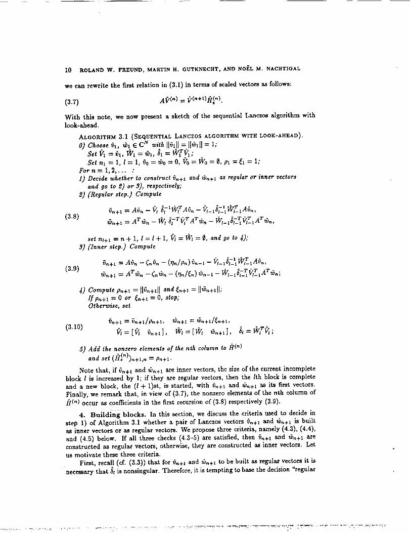
10 ROLAND W. FREUND, MARTIN H. GUTKNECHT, AND NOF, L M. NACHTIGAL

we can rewrite the first relation in (3.1) in terms of scaled vectors as follows:

(3.7) At'(">= _("+_>_.(").

With this note, we now present a sketch of the sequential Lanczos algorithm withlook-ahead.

ALGORITHM 3.1 (SEQUENTIAL LANCZOS ALGORITHM WITH LOOK-AHEAD).

O) Choose _1, _1 _ cH with 116_11= I1,_11= 1;

Set _, = _1, e¢_= _1, _, = _;Set nl = 1, I= 1, % = _o =0, f'o = Wo = 0, pl =¢1 = 1;

For n = 1,2,... :

1) Decide whether to construct fYn+l and fu_+l as regular or inner vectorsand go to 2) or 3), respectively;

8) (Regular step.) Compute

(3.8)ffJ.+1= AT_on- l_l _f-Tqr AT6o_- l;Vt_l_,-_ _T1ATfort,

set nt+l -- n + 1, I = I + 1, _ = _ = _, and go to 4);

3) (Inner step.) Compute

(3.9)wn+l = AT tbn-_ntbn - (Tln/_n)ton-1-- V_rl_I$_ZVIT_IAT_bn;

4) Computep.+l --I1_-+1tland_n÷l -" 11_,,÷111;Ifpn+l = 0 or _'n+l = O, stop;

Otherwise, set

'_n+l "-- Yn+l/Pn+l, 11)n+1 "-- _n+l/_Cn+l,

(3.10) _-'[_ @n+z], lfid,-"[l'_ r` t_,_+l], _,=l';¢trq;

5) Add the nonzero elements of the nth column to It(")

,,.d set (._.(")),,+1,.= p.+_.

Note that, if 6,,+1 and _.+1 are inner vectors, the size of the current incomplete

block I is increased by 1; if they are regular vectors, then the lth block is completeand a new block, the (l + 1)st, is started, with T),+I and tb,+l as its first vectors.

Finally, we remark that, in view of (3.7), the nonzero elements of the nth column of

/f('_) occur as coefficients in the first recursion of (3.8) respectively (3.9).

4. Building blocks, in this section, we discuss the criteria used to decide in

step 1) of Algorithm 3.1 whether a pair of Lanczos vectors _3,+_ and _b,_+l is built

as inner vectors or as regular vectors. We propose three criteria, namely (4.3), (4.4),

and (4.5) below. If all three checks (4.3-5) are satisfied, then fi,_+_ and d_n+_ are

constructed as regular vectors, otherwise, they are constructed as inner vectors. Letus motivate these three criteria.

First, recall (cf. (3.3)) that for *)n+l and tb,+_ to be built as regular vectors it is

necessary that $_ is nonsingular. Therefore, it is tempting to base the decision "regular


versus inner step" solely on checking whether _l is close to singular, and to perform a

regular step if, and only if,

(4.1) O'min (_l(n)) _> tol,

for some suitably chosen tolerance tol. For example, Parlett [22] suggests tol = e 114

or tol = el/a, where e denotes the roundoff unit. Then (4.1) would guarantee that

complete blocks of computed Lanczos vectors satisfy

_min(ak) > tot, t = 1,2,....

This, together with (3.3), would imply by [22, Theorem 10.1] that

tol tol(4.2) O'min (I/(n)) > _ and Crmin(I,V (")) > "-_, n = n_ - 1, k = 1,2, ....

Vn v"

Since the columns of _'(") and IYc'(n) are unit vectors, O'min (_r(n)) and amin (I_¢'(n)) are

a measure of the linear independence of these vectors; in particular, (4.2) would ensure

that the Lanczos vectors remain linearly independent. However, in the outlined algo-

rithm, the block orthogonality (3.2-3) is enforced only among two or three successive

blocks, and in finite precision arithmetic, biorthogonality of blocks whose indices are

far apart is typically lost. The theorem assumes that (3.2-3) hold for all indices, and

without this, the theorem fails in finite arithmetic. We illustrate this with a simple

example.

Example $.1. In Figure 4.1, we plot O'rnin ($1(n)) (dots), minx<t<l(n)(O'min (_k))

(solid line), and v/-ff _rmin (V(")) (dotted line), as functions of the iteration index

n = 1, 2,..., for a random 50 × 50 dense matrix. The theorem predicts that

V/_ O.mi n (_,r(n)) _ x_<k<tCn)(minO'min (_)),

which is clearly not the case.

As this simple example shows, the check (4.1) alone does not ensure that the

computed Lanczos vectors are sufficiently linearly independent. In particular, if thelook-ahead strategy is based only on criterion (4.1), the algorithm may produce withina block Lanczos vectors which are almost linearly dependent. When this happens, the

check (4.1) usually fails in all subsequent iterations and thus the algorithm never

completes the current block, i.e., it has generated an artificial incurable breakdown.In addition, numerical experience indicates another problem with (4.1): for val-

ues of tol which are "reasonably" larger than machine epsilon, the behavior of the

algorithm is very sensitive with respect to the actual value of toi. We also illustrate

this with an example.

Example _._. We applied the Lanczos algorithm to a nonsymmetric matrix A

obtained from discretizing a 3-D partial differential equation (eft Example 6.4 in

Section 6). This example was run on a machine with e _ 1.3E-29. In the first case,

we set tol = e 114 ._. 6.0E-08, while in the second case, we set tol = e113 _ 2.3E-10.

In Figure 4.2, we plot _min (Sa(,)) versus the iteration index n for the two runs, thedotted line for e 114 and the solid line for e1/3. In the first case, the algorithm starts

building a block which it never closes, and the singular values clearly become smallerand smaller. Yet if tol is only slightly smaller, as in the second case, the algorithm

12 ROLAND W. FREUND_ MARTIN H. GUTKNECHT, AND NOEL M. NACHTIGAL

runs to completion, in this case solving the linear system to the desired accuracy, and

thus indicating that the block built in the first case was not a true, but an artificialincurable breakdown.

We note that the sensitivity of look-ahead procedures to the choice of tolerances,

such as tol in (4.1), was also observed in [5]. However, no remedy for this phenomenon

is given in [5]. Furthermore, we remark that the problem of generating almost linearly

dependent vectors is not specific to the Lanczos biorthogonaiization process. Indeed,similar effects can also occur in true orthogonalization methods (of. [27]).

Examples 4.1 and 4.2 clearly show that the decision "regular versus inner step"

cannot be based on (4.1) alone. Instead, we propose to relax the check (4.1), so that

it merely ensures that St(,,) is numerically nonsingular, and to add the checks (4.4-5)below which guarantee that the computed Lanczos vectors remain sufficiently linearly

independent. Hence, instead of (4.1), we check for

(4.3) O'min (St(n)))_ •,

where • denotes the roundoff unit.

Our numerical experiments have shown that typically the algorithm starts to gen-erate Lanczos vectors which are almost linearly dependent, once a regular vector _,+1

was computed whose component At3, E K,+l(Vl, A) is dominated by its componentin the previous Krylov space Kn(vl,A) (and similarly for tb,+t). In order to avoid

the construction of such regular vectors, we check the/t-norm of the coefficients for

_-I and _ in (3.8); _,+t can be computed as a regular vector only if

j=n*-I j=n_

Here n(A) is a factor depending on the norm of A; we will indicate later how thisfactor is computed. Similarly, we check the/t-norm of the coefficients for I)fl_t and

l_l in (3.8); w,_+l can be computed as a regular vector only if

rl

.t-I A--T A T TI_(4.5) E [ (_/-IV/-1A n)Jl -_ n(A) and E (_['T_'ITATu)n)J __n(A).

j=n,-I j=n_

The pair _,,+t and tb,+t is built as regular vectors only if the checks (4.3-5) hold true.We need to indicate how n(A) is chosen in (4.4-5). Numerical experience with

matrices whose norm is known indicates that setting n(A) = HAl) is too strict and canresult in artificial incurable breakdowns. A better setting seems to be n(A) = 10. HAll,

but even this is dependent on the matrix. In any case, in practice one does not know

HAH, and there is also the issue of a maximal block size, determined by limits onavailable storage. To solve the problems of estimating the norms and a suitable factor

n(A), as well as cope with limited storage and yet allow the algorithm to proceed asfar as possible, we propose the following procedure. Suppose we are given an initial

value for n(A), based either on an estimate from the user (for example, n(A) from a

previous run with the matrix A), or by setting

n(A) -- max ([]A_xll, [IAT tI[}•


Note that here A denotes the matrix actually used in generating the Lanczos vectors,

thus including the case when we are solving a preconditioned linear system. We then

update n(A) dynamically, as follows. In each block, whenever an inner vector is built

because one of the checks (4.4-5) is not satisfied, the algorithm keeps track of the size

of the terms that have caused one or more of (4.4-5) to be false. If the block closesnaturally, then this information is not needed. If, however, the algorithm is about to

run out of storage, then n(A) is replaced with the smallest value which has caused an

inner vector to be built. The updated value of n(A) is guaranteed to pass the checks

(4.4-5) at least once, and hence the block is guaranteed to close. This also frees up

the storage that was used by the previous block, thus ensuring that the algorithm canproceed.

5. Implementation details. We now turn to a few implementation details.

In particular, we wish to show how one can implement the sequential algorithm with

the same number of inner products per step as the classical Lanczos algorithm. For a

regular step, one needs to compute $1, I)VTA_,, and I]¢'TIA_, in (3.8). For an inner

step, one needs to compute I)/T i A)), in (3.9) and to update 6_ in (3.10). We will show

that for a block of size hj, only 2hi inner products are required: 2ht-1 will be required

to compute 6_, and one inner product will be required to compute [_'TA_,. We will

obtain _ 1A_,_ without performing any inner products. To simplify the derivations,

we will use the "monic" vectors vn and wn. All quantities involving the scaled vectors

_in and tbn can be obtained from the corresponding quantities involving vn and w,

simply by scaling. Finally, we remark that, using a similar argument as in (5.1) below,

one easilyverifiesthat

WTAvn = VirATw,_ and WT1Avn = VIT_IATWn.

Therefore, the coefficients 6_'T_TATtb, and 67.T1_TiAr_b,, , which occur in the recur-

sions for the left Lanczos vectors in (3.8) or (3.9), can be generated from 671WTA_and "-I " r_I-i W__ tA_),, without computing any additional inner products.

Consider first 61. Using (2.9) and the fact that polynomials in A commute, wededuce that

(5.1) wri vj -- wT@i(A)qtj(A)vl - wT_lj(A)_ti(A)vl = wTv,.

This shows that the matrix 6a is symmetric, and hence we only need to compute its

upper triangle.

We will now show that once the diagonal and first superdiagonal of _ft have been

computed by inner products, the remaining upper triangle can be computed by recur-

rences. Let wi and vi be two vectors from the current block. Using (3.6) and the factthat the inner vectors from block I are orthogonal to the vectors from the previous

block, we have

14 ROLAND W. FItEUND, MARTIN H. GUTKNECHT, AND NOEL M. NACHTIGAL

Thus, wTv j depends only on elements of 6t from the previous two columns, and hence,with the exception of the diagonal and the first superdiagonal, can be computed with-

out any additional inner products. Note that the recurrences and the orthogonality

used in the above derivation are enforced numerically, and so computing wTvi by the

above recurrence should give the same results - up to roundoff - as computing the

inner product directly ....We will now show how to compute W_TAvn with only one additional inner product/-

while W_l_lAvn can be obtained with no additional inner products. Consider wTAvn,for w_ a vector from either the current or the previous block.

toTi Avn -- (AT toi)T _n "- (tOi÷l q" _itlYi "J" 17iWi-1)T Vn

= + +

For i < nt- 1, W_rz_lv_, = 0, and hence wTAv,_ = O. For i = hi-l, the above

reduces to wT,_tAvn = w_,v,, which is computed as part of the first row of 61. Fornt < i < n,+l, all of the terms needed are available from 6:. Finally, for the last vector

in the current block, i = nr+l - 1, we do not have wrn,+, v,_, and hence have to computeit directly, thus requiring another inner product.

6. Numerical examples. We have performed extensive numerical experiments

with our implementation of the look-ahead Lanczos algorithm, both for eigenvalueproblems and for the solution of linear systems. In this section, we present a few

typical results of these experiments. Further numerical results are reported in [1 1]

and [12].Approximations to the eigenvalues of A can be obtained from the look-ahead

Lanczos algorithm by computing some or all of the eigenvalues of the Lanczos matrix

/7/("), the so-called Ritz values. In general, spurious approximate eigenvalues can oc-

cur among the Ritz values. We have used the heuristic due to Cullum and Willoughby

[6] to identify and eliminate spurious Ritz values. Although this procedure was origi-

nally proposed for the scalar tridiagonal matrices generated by the standard Lanczos

process, we also found it to work satisfactorily for the block tridiagonal matrices/_('_)

produced by the took-ahead Lanczos algorithm. The eigenvalues of H('_) were always

computed using standard EISPACK routines.

For the solution of nonsingular linear systems

(6.1) Az = b,

we combine the look-ahead Lanczos algorithm with the QMR approach. More pre-

cisely, let z0 _ C N be any initial guess for (6.1) and choose the normalized startingresidual vector

t_l := ro/Po, ro := b- Azo, Po :- Ilr01l,

as the first right Lanczos vector in Algorithm 3.1. The QMR method then generates

approximate solutions to (6.1) defined by

(6.2) z, = z0 + !_'(")z,, n = 1,2,... ,

where z,, is the solution of the least squares problem


We remark that,using (3.7),one easilyverifiesthat the residualvectorcorresponding

to the iterate(6.2)satisfies

(6.4)/

r,,:-"b - .4z,_= tp0e,-\--

Thus the choice(6.3)of zn justguarantees that the Euclidean norm of the coefficient

vectorinthe representation(6.4)isminimal. For detailsand furtherpropertiesof the

QMR method, we referto [12].

Example 5.1. This examples isan eigenvalueproblems, taken from [6].Consider

the differentialoperator

(6.s)

+2o(x+ + ((x+y).)+1

U

l+z+y

on the unit square (0, 1) x (0, 1). We discretize (6.5) using centered differences on

a 29 x 29 grid with mesh size h -- 1/30. This leads to a nonsymmetric matrix of

order N = 900. In Figure 6.1, we plot the Ritz values (marked by '%') generatedby the look-ahead Lanczos process after n = 40, 80, 160, 320 steps. We note that

after 40 steps, the complex conjugate pair of Ritz values with maximal real part had

converged to eigenvalues of A. After 80 steps, 12 Ritz values (all on the right edge of

the spectrum) had converged, while after 160 steps the 30 Ritz values (24 on the right

edge and 6 on the left edge of the spectrum) had converged to eigenvalues of A. Forthis example, we have used unit vectors with random coefficients as starting vectors

61, _bl for Algorithm 3.1.

Ezample 6._. This example is an eigenvalue problem, taken from [23], whose exact

eigenvalues are known. Generally, problems of this type arise in modeling concentra-tion waves in reaction and transport interaction of chemical solutions in a tubular

reactor. The particular test problem used here corresponds to the so-called Brussela-

tor wave model. This example was run for a matrix A of size N = 100. The look-aheadLanczos algorithm needs n = 112 steps to obtain all the eigenvalues of A; it builds

2 blocks of size 2. For this example, we have also run the standard Lanczos process

without look-ahead, and computed the Ritz values after n = 100, 112, 120 steps. Thedenominators _bsztb,_ were checked to exceed v/_ in magnitude. In all three cases, some

of the Ritz values obtained from the standard Lanczos process after deleting spuriousand ghost eigenva]ues do not correspond to any of the eigenvalues of A. In particular,

the standard Lanczos process does not obtain the smallest eigenvalues of A even after

120 steps, and generates incorrect Ritz values, as shown in the plot. In Figure 5.2,

we plot the Ritz values generated by the look-ahead Lanczos process (marked by "o")

and the Ritz values generated by the standard Lanczos process (marked by "+'), both

after 120 steps.Example 6.3. Here we consider a 6-cyclic matrix

(6.6) A = ,0000)11B2 /2 0 0 00 B3 /'3 0 0

0 0 B4 /4 0

0 0 0 B5 Is

0 0 0 0 Bs /'6 J


where the diagonal blocks I1, I2, I3, I4, Is, and Ie are identity matrices of size

827, 844, 827, 838, 831, and 838, respectively, so that A is a matrix of order

N = 5005. This matrix arises in Markov chain modeling. For general p-cyclic ma-

trices A of the form (6.6), Freund, Golub, and Hochbruck [9] have shown that work

and storage of the look-ahead Lanczos process can be reduced to approx/mately lip,as compared to arbitrary starting vectors, if vt and wt have only one nonzero block

conforming to the block structure of A. Here, we have chosen

0,- o,--where fl, gl E Rs2_'have random entries.The look-aheM Lanczos algorithm generates

blocks that alternatelyhave sizesi and 5,startingwith a block ofsizeI.In Figure 6.3,

we plot the Ritz values(marked by "o') generated by the look-ahead Lanczos process

afterr_= 40, 80, 160, 320 steps.The standard Lanczos algorithm without look-ahead

generates one Ritz value 1 inthe firststep,and then breaks down in the second step.

Clearly,thisexample shows that the use oflook-ahead iscrucialifone wants toexploit

the specialstructureofp-cyclicmatrices.

Example 6.4. Here we consider the partial differential equation

(6.7) Lu=f on (0,1) x(0,1)x(0,1),

where

\ ox/- \ ov/- \ o;,/

( , )+_(z+Y+z)ox+ ?+ l+z+y+z u,

with Dirichlet boundary conditions u = 0. The right-hand side f is chosen such that

u--(1-z)(1-y)(1-z)(1-e -z)(1-e -y) (l-e-')

is the exact solution of (6.7). We set the parameters in (6.7) to/3 = 30 and 7 = -250,and then we discretize (6.7) using centered differences on a uniform 15 x 15 x 15 grid

with mesh size h = 1/16. This leads to a linear system (6.1) with coefficient matrix

A of order N = 3375 and 22275 nonzero elements. For the first left Lanczos vector,

we have chosen *hi = t31 in Algorithm 3.1. The QMR approach takes n = 149 stepsto reduce the norm of the initial residual by a factor of 10-6; see Figure 6.4, where

the relative norm lit, I!/I[r011 is plotted versus n (solid line). Finally, we note that the

matrix A is just the one used in Example 4.2. Recall that the look-ahead Lanczos

algorithm based on the check (4.1) with tolerance tol = _t/4 _ 6.0E-08 encountered

an artificial incurable breakdown. We also ran QMR based on this version of the

look-ahead Lanczos algorithm, and the resulting convergence curve is shown as the

dotted line in Figure 6.4. Notice that,_due tp the artificial_incurable breakd0wn ' QMR

does not converge in this case (cf. Figur e 4.2). __ _

7. Conclusion. We have proposed an implementation of tlae look-ahead Lanczos

algorithm for non-Hermitian matrices. Our implementation can handle look-ahead

steps of any length. Also, the proposed algorithm requires the same number of innerproducts as the standard Lanczos process without iook-aheM. It was our intention to

develop a robust algorithm which can be used in a:blackbox.

FORTRAN 77 codes ofour implementation ofthe look-aheM Lanczos algorithm

and the QMR method are availableelectronicallyfrom the authors (na.freund@na-

net.ornl.govor [email protected]).


Acknowledgments. Part of thiswork was done while the firstand thirdauthor

were visitingthe InterdisciplinaryProjectCenter forSupercomputing at ETH Zfirich,

and we thank Martin Gutknecht for hiswarm hospitality.The authors are grateful

to Marlis Hochbruck for her help with Example 6.3 and her carefulreading of the

manuscript.

REFERENCES

[1] D.L. BOLEY, S. ELHAY, G.H. GOLUB, AND M.H. GUTKNECHT, Nonsymmetri¢ Lanczos and

finding orthogonal polynomials associated witlt indefinite weight,, Numer. Algorithms, 1

(1991), pp. 21--43.

[2] D.L. BOLEY AND G.H. GOLUB, The nonsymmetric Lanczos algorithm and controllability,

Systems Control Lett., 16 (1991), pp. 97-105.

[3] C. BREZINSZI, Pad4-Type Approximation and General OrtAogonM Polynomials, Birkh_user,

Basel, 1980.

[4] C. BREZINSKI, M. REDIVO ZAGLIA, AND H. SADOK, A breakdown-free Lanczos type algorithm

for solving linear systems, Numer. Math. (to appear).

[5] _, Avoiding breakdown and near-breakdowns in Lanczos type algorithms, Preprlnt,

Universit_ des Sciences et Techniques de Lille Flandres-Artois, France, 1991.

[6] J. CULLUM AND R.A. WILLOUGHBY, A practical procedltre for e0mp_ding eigenval_es of laws

sparse nonsJ/mmetric matrices, in Large Sca/e EigenvaJue Problems, J. Cu]]um and R.A.

Willoughby, eds., North-Holland, 1986, pp. 193-240.

[7] A. DRAUX, Polyndme_ Or_/Logona_.z Formula - Applications, Lecture Notes in MfathemaHcs,

Volume 97_, Springer, Berlin, 1983.

[8] R.W. FREUND, Conjugate gradient type methods for linear systems with complez slmmetric

coe.O_cient matrices, SIAM J. Sci.Stat. Comput., 13 (1992) (to appear).

[9] R.W. FREUND, G.H. GOLUB, AND M. HOCHBRUCK, Krylo_ sub#pace method# for non-Hermi-

tian p-el:cite matrices, Technical Report, RIACS, NASA Ames Research Center, in prepa-

ration.

[10] R.W. FREUND, M.H. GUTMNF_X3HT, AND N.M. N^CHTIGAL, An implementation of tar look-

ahead Lanczos algorithm for non-Herraltian matrices, P_rt [, Technical Report 90.45,

RIACS, NASA Ames Research Center, November 1990.

[11] R.W. FR_.UND AND N.M. NAcHTTGAL, An implementation of the look-altead Lanezo* algo-

rithm loI" non-Hermitian matrices, Part II, Technical Report 90.46, RIACS, NASA Ames

Research Center, November 1990.

[12] --, QMR: a quasi-minimal residual method for non-Hermltian linear system*, Numer.

Math. (to appear).

[13] W.B. GRAGG, Matriz interpretations and applications of the continued fraction algorithm,

Rocky Mountain ,7. Math., 4 (1974), pp. 213-225.

[14] W.B. GRAGO AND A. LINDQUIST, On the partial realization problem, Linear Algebra Appl.,

50 (1983), pp. 277-319,

[15] M.H. GUTKNECHT, A completed theory of the Insymmetric Lanczos process and related algo-

rithms, Part I, SIAM J. Matrix Anal. Appl. (to appear).

[16] , A completed theorT/ of the unsymmetric L,tnezos process and related algorithms, Part

[[, 1PS Research Report No. 90-16, ZCtrich, Switzerland, September 1990.

[17] W. JOUBERT, Lanczos methods/or the solution of nons_mmctric systems of linear equations,

in Proceeding_ of the Copper Mountain Conference on Iterative Methods, April 1-5, 1990.

[18] S. KUNG, M_ltivariable and m,Jltidimensional systems: analysis and design, Ph.D. Disserta-

tion, Stanford University, Stanford, June 1977.

[19] C. LANCZOS, An iteration method for the solution of the eigennalne problem of linear di_er-

ential and integral oper, tors, J. Res. Nat. Bur. Standards, 45 (1950), pp. 255-282.

[20] , Solution of systems of linear equationJ by minimized iterations, J. Re#. Nat. Bur.

Standards, 49 (1952), pp. 33--53.

[21] T.A. MANTEUFFEL, The Tcl_eb_che*, iteration ?or nonsymmetric linear system#, Numer.

Math., 28 (1977), pp. 307'-327.

[22] B.N. PARL_r'r, Reduction to tridiagonal form and minimal realizations, Preprint, University

of California, Berkeley, January 1990.

18 ROLAND W. FREUND, MARTIN H. GUTKNECHT, AND NOP.L M. NACHTIGAL

[23] B.N. PARLEI"r AND Y. SAAD, Comple= shift and inver_ jtr_|egles/or real m6_r/cea, Linear

Algebra Appl., 88/89 (1987), pp. 575-595.

[24] B.N. PARLETr, D.R. TAYLOR, AND Z.A. LIu, A look-ahe4d Z_nczos 6loorlthm for ttnaFmmefric

mstT/_a, Math. Comp., 44 (1985), pp. 105-124.

[25] E.L. STIEFEL, Kernel polynomialJ in linear _Ioebr6 6nd their n_meric41 applie_fionJ, U.$.

Nations] Bureau of Standards, Applied Mathematics Series, 49 (1958), pp. 1-22.

[26] D.R. TA_'_R, A_41y#i# o/the look 6he_d L4nczo# algo_hm, Ph.D. Dissertation, University

of Ca/iforni&, Berkeley, November 1982.

[27] H.F. WALKER, Implemen_afion o/ the GMRES method eaing Hosleholder fr_nJform_Zions,SIAM J. Sci. St, at. Comput., 9 (1988), pp. I52-16.3.

[28] J.H. WILKINSON, The Algebraic Eigeneelee Problem, Oxford University Press, Oxford, 196,5.

AN IMPLEMENTATION OF THE LOOK-AHEAD LANCZOS ALGOEITHM 19

10 7

104

101

10-2

10-5

10-8

10-11

10-14

,. ,, o o o,,,., ._, " . "

• ,,', °% • "o "%-* • +.. • •o • • ,o o- .

• ,. %." . °o o.

;'.."...*'..., ...-. ....... , ....

lO-t7 0 2'o

.. ........ o,

.....,....'"""

.,.....-..-'" ""

• ",--... +,, ,..+..."'

'.+-

I I I

40 60 80 I00

Figure 4.1. _rnia (_t(,,)) (dots), minl<k<l(n) (_min (6k)) (solid line), and

_min (Q(n)) (dotted Hne), plotted versus the iteration index n

20 ROLAND W. FREUND, MAP.TIN H. GUTKNECHT, AND NOF, L M. NACHTIGAL

10 4

10-3

lO-iO

10-17

10-24

10-31o

t

\

;o 1;o 15o

Figure 4.2. _1/4 (dottedline) and e1/3 (solid line), plotted

versus the iteration index n

AN IMPLEMENTATION OF THE LOOK-AHEAD LANCZO$ ALGORITHM

2

1

0

-1

-20

After 40 steps

0 O0 00 0 0 0 O0

0 00

0 0 0

o oo

0 oo

0o o

o o °o°o Ooo

10

2 o After 80 steps

I o_°o _°°°o °

p/oo+°+.7oO0 o o

,_o+oooOOO+ +oo o

i_o o +0o:oo'° i0

21

2

1

0

-1

-20

After 160 stepsi

_l) O0 0 0

a_ o0 oO o

._.._.o oo

oI

5

2

1

0

10 10

After 320 stepso

¢1_ o °

o oo__ oO°;ooo,oo*

o

_ooq) o o

o

0 ;

Figure 6.1. Ritz values for Example 6.1, obtained alter n = 40, 80, 160, 320 steps

of the look-ahead Lanczos algorithm

22 ROLAND W. FREUND, MARTIN H. GUTKNECHT, AND NOEL M. NACHTI(3AL

5

4

3

2

1

0

-1

-2!

_it-350

D,

I0

X

]Cx

_DBB• • • • • • M • • • • • • •__•BBUOg_i_B_ X

X

X

X

0X

-3_o -_o -2_ -1_o -1_ -;o

;$

l$"

i

0

i

Figure 6.2. l_tz values (marked by "o" respectively "-I-") for Example 6.2, obtained

from the look-ahead respectively standard Lmacztm a_gorithm

AN IMPLEMENTATION OF THE LOOK-AHEAD LANCZOS ALGORITHM

1

0.5

0

-0.5

-10

o_t_" _ st_p_o 1o 0

oo 0 o

o 0

0 0

o

0 o

o 0

o 0o o

0 0

o n i n o

1 2

0.5

o

0 _o°°o

° 0

-0.5

_°oI

"i0 I

After 80 steps

_OoOoOo oo_

0 0 0 0

0

o 0o8

o

oo

0 o o

°_

23

I

0.5

0

-0.5

-10

After 160 steps

'_.oooo8 o_oo?o#_ ° °o_ o

oo oo

/o"\o o o:

o_,o_I

1

After 320 steps1

0.5

0,

-0.5

2 0 1

.(o% #

Figure 6.3. Ritz values for Example 6.3, obtained after n = 40, 80, 160, 320 steps

of the look-ahead Lanczos algorithm

24 ROLAND W. FREUND, MAP.TIN H. GUTKNECHT, AND NOEL M. NACHTIGAL

10o , ,

10-1

10-2

10-3

10-4

10-5

10.5

J

1°-'0 ._ 1_o 15o

Figure 6.4. Rel_tive r_sidu_a .o_m II_-II/I1_011plottedversus r_, for Example 6.4

an implementation of the look-ahead lanczos algorithm for ... · an implementation of the...

Documents