an implementation of model-free face detection and...

An Implementation of Model-Free Face Detection and Head Tracking with Morphological Hole

Mapping in C#

ENCM 503: Digital Video Processing Department of Electrical and Computer Engineering

Schulich School of Engineering University of Calgary

Paul Lapides Charles Hateley

December 7, 2007

Table of Contents Abstract ............................................................................................................................... 1

Procedure ............................................................................................................................ 1

Binary Skin map ............................................................................................................. 2

RGB skin clustering.................................................................................................... 2

YCrCb skin clustering................................................................................................. 2

HSV skin clustering .................................................................................................... 3

Observations ............................................................................................................... 3

Morphological Face Extraction....................................................................................... 3

Closing the Skin Regions............................................................................................ 3

Dilation ....................................................................................................................... 4

Erosion ........................................................................................................................ 4

Hole map..................................................................................................................... 4

Labeling ...................................................................................................................... 5

Identify Faces.................................................................................................................. 7

Limitations and Improvements ........................................................................................... 8

Lighting Conditions ........................................................................................................ 8

False Positives and Recognition Problems ..................................................................... 9

Imperfect Closing............................................................................................................ 9

Speed............................................................................................................................. 10

Credits ............................................................................................................................... 10

Abstract This project implements face detection and tracking using morphological methods as

outlined by [1]. An interactive C# program was developed which uses a supplied camera

interface [5] for acquiring image data. This interface was the only library used in the

implementation – image-processing functionality was implemented specific to the classes

defined in the project.

The proposed method fares quite well at detecting faces in varying conditions as well the

tracking there of. The hole-mapping method successfully detects faces at most rotational

angles as long as some face is showing.

Procedure The algorithm we implemented finds face regions by examining the number of “holes”

(e.g. eyes, nose, mouth, ears) in each region. If the number of holes is above a threshold,

the region is considered a face.

Regions are created by applying a simple set of rules to each pixel in the image [1]. These

rules determine if the pixel is skin colored and should be considered further. This creates

a black & white image (not grayscale) of candidate skin regions.

Some regions will have black holes inside of them that could be eyes, nose, etc and need

to be isolated. To isolate, the skin regions are “closed”, which means that these holes are

filled in. Closing is done by two similar operations called dilation and erosion [2,3]. Once

the holes are closed, the original skin regions are subtracted from the closed regions,

leaving only the holes.

Both the skin and hole regions are then labeled, which assigns connected regions a

unique tag [4]. The labeled hole image is overlaid above the labeled image and the

number of holes above each labeled region are counted. The labeled regions with the

most holes are considered faces and are enclosed with a rectangle.

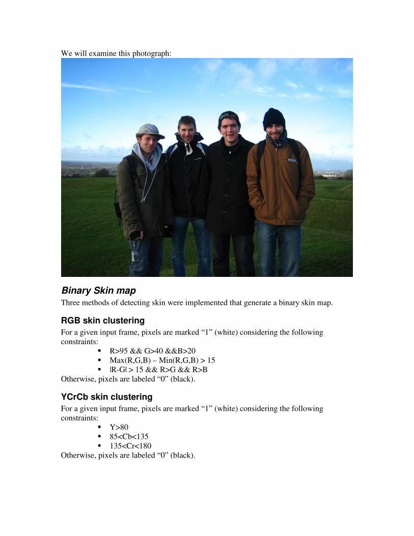
We will examine this photograph:

Binary Skin map

Three methods of detecting skin were implemented that generate a binary skin map.

RGB skin clustering

For a given input frame, pixels are marked “1” (white) considering the following

constraints:

� R>95 && G>40 &&B>20

� Max(R,G,B) – Min(R,G,B) > 15

� |R-G| > 15 && R>G && R>B

Otherwise, pixels are labeled “0” (black).

YCrCb skin clustering


constraints:

� Y>80

� 85<Cb<135

� 135<Cr<180


HSV skin clustering


constraints:

� 0<H<50

� 0.23<S<0.68


Observations

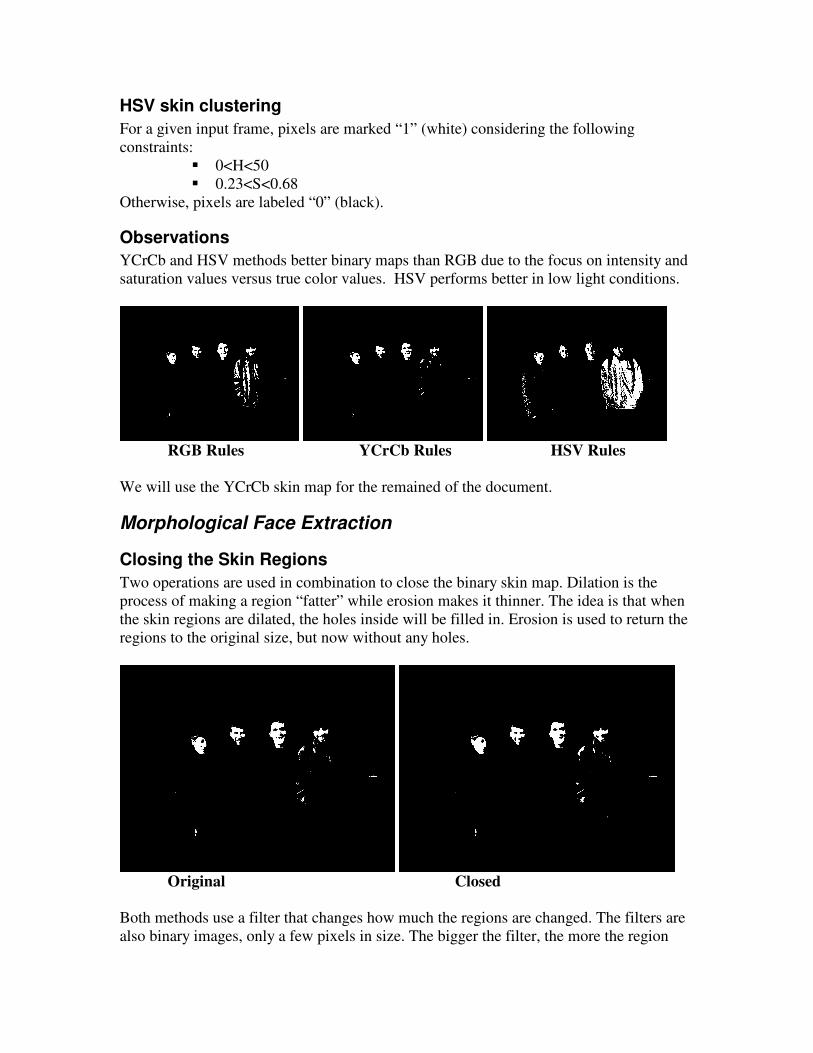
YCrCb and HSV methods better binary maps than RGB due to the focus on intensity and

saturation values versus true color values. HSV performs better in low light conditions.

RGB Rules YCrCb Rules HSV Rules

We will use the YCrCb skin map for the remained of the document.

Morphological Face Extraction

Closing the Skin Regions

Two operations are used in combination to close the binary skin map. Dilation is the

process of making a region “fatter” while erosion makes it thinner. The idea is that when

the skin regions are dilated, the holes inside will be filled in. Erosion is used to return the

regions to the original size, but now without any holes.

Original Closed

Both methods use a filter that changes how much the regions are changed. The filters are

also binary images, only a few pixels in size. The bigger the filter, the more the region

will be dilated or eroded. A circle was used in our implementation, but a square will be

used in the explanations to follow.

Dilation

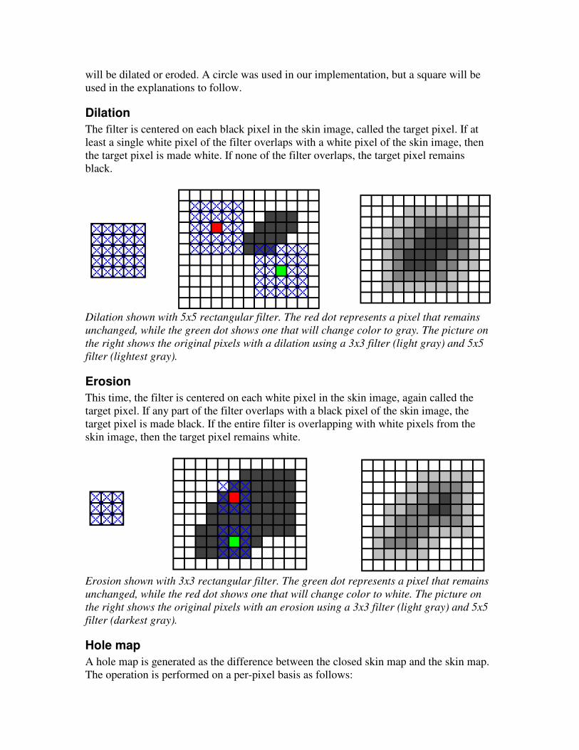
The filter is centered on each black pixel in the skin image, called the target pixel. If at

least a single white pixel of the filter overlaps with a white pixel of the skin image, then

the target pixel is made white. If none of the filter overlaps, the target pixel remains

black.

Dilation shown with 5x5 rectangular filter. The red dot represents a pixel that remains

unchanged, while the green dot shows one that will change color to gray. The picture on

the right shows the original pixels with a dilation using a 3x3 filter (light gray) and 5x5

filter (lightest gray).

Erosion

This time, the filter is centered on each white pixel in the skin image, again called the

target pixel. If any part of the filter overlaps with a black pixel of the skin image, the

target pixel is made black. If the entire filter is overlapping with white pixels from the

skin image, then the target pixel remains white.

Erosion shown with 3x3 rectangular filter. The green dot represents a pixel that remains

unchanged, while the red dot shows one that will change color to white. The picture on

the right shows the original pixels with an erosion using a 3x3 filter (light gray) and 5x5

filter (darkest gray).

Hole map

A hole map is generated as the difference between the closed skin map and the skin map.

The operation is performed on a per-pixel basis as follows:

Equation 1

),(),(),( yxPyxPyxP SkinCSkinhole −=

The result is a new binary image representing the “holes” in the skin regions.

Labeling

Each skin and hole region must be labeled so it can be treated as a single unit instead of

simply a group of connected pixels. Labeling is done by assigning unique tags (numbers)

to each pixel in the image. Black pixels are given a tag of 0, while white pixels have tags

that are greater than zero, kept track with a counter that is incremented.

The image is scanned left to right, row by row. Only white pixels are considered for

tagging. A target pixel will have four neighbors that have already been tagged. The left,

up-left, up, and up-right will be used to assign a tag to the target pixel. There are three

possible cases that can occur.

The first case is if none of the neighbor pixels are white. The neighbors will all have tags

of 0. A new unique tag is assigned to the target pixel using the value of the counter. The

counter is incremented.

The second case is if only one of the neighbor pixels is white. This neighbor will have a

non-zero tag that will be assigned to the target pixel since the two pixels are touching

(they are neighbors).

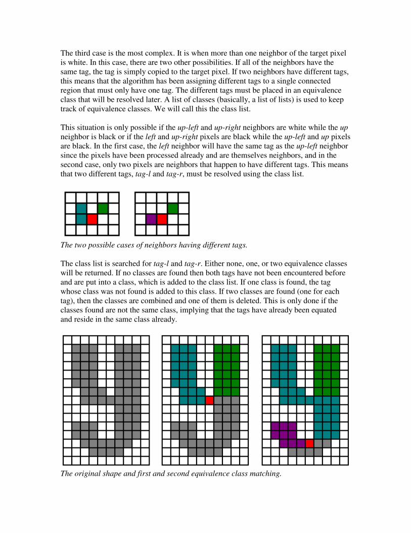
The third case is the most complex. It is when more than one neighbor of the target pixel

is white. In this case, there are two other possibilities. If all of the neighbors have the

same tag, the tag is simply copied to the target pixel. If two neighbors have different tags,

this means that the algorithm has been assigning different tags to a single connected

region that must only have one tag. The different tags must be placed in an equivalence

class that will be resolved later. A list of classes (basically, a list of lists) is used to keep

track of equivalence classes. We will call this the class list.

This situation is only possible if the up-left and up-right neighbors are white while the up

neighbor is black or if the left and up-right pixels are black while the up-left and up pixels

are black. In the first case, the left neighbor will have the same tag as the up-left neighbor

since the pixels have been processed already and are themselves neighbors, and in the

second case, only two pixels are neighbors that happen to have different tags. This means

that two different tags, tag-l and tag-r, must be resolved using the class list.

The two possible cases of neighbors having different tags.

The class list is searched for tag-l and tag-r. Either none, one, or two equivalence classes

will be returned. If no classes are found then both tags have not been encountered before

and are put into a class, which is added to the class list. If one class is found, the tag

whose class was not found is added to this class. If two classes are found (one for each

tag), then the classes are combined and one of them is deleted. This is only done if the

classes found are not the same class, implying that the tags have already been equated

and reside in the same class already.

The original shape and first and second equivalence class matching.

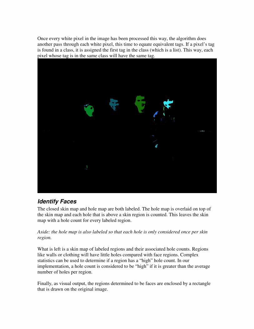
Once every white pixel in the image has been processed this way, the algorithm does

another pass through each white pixel, this time to equate equivalent tags. If a pixel’s tag

is found in a class, it is assigned the first tag in the class (which is a list). This way, each

pixel whose tag is in the same class will have the same tag.

Identify Faces

The closed skin map and hole map are both labeled. The hole map is overlaid on top of

the skin map and each hole that is above a skin region is counted. This leaves the skin

map with a hole count for every labeled region.

Aside: the hole map is also labeled so that each hole is only considered once per skin

region.

What is left is a skin map of labeled regions and their associated hole counts. Regions

like walls or clothing will have little holes compared with face regions. Complex

statistics can be used to determine if a region has a “high” hole count. In our

implementation, a hole count is considered to be “high” if it is greater than the average

number of holes per region.

Finally, as visual output, the regions determined to be faces are enclosed by a rectangle

that is drawn on the original image.

Limitations and Improvements

Lighting Conditions

The rules for identifying skin are based entirely on color. When a poorly lit image is

captured, the colors of the skin pixels are not the same as in a well lit image. Because of

this discrepancy, skin regions are not correctly identified if the image is too dark.

A value can be computed based on the average brightness or contrast of the image that

can be used to adjust the values used in the skin rules.

False Positives and Recognition Problems

Regions that are not faces are sometimes incorrectly identified as faces. This is because

the region is skin colored and has a high number of holes – the exact metrics we use to

detect faces. For example, an arm with a tattoo or a beige colored shirt with a graphic will

be considered skin while the tattoo and graphic will not, creating holes. This will

contaminate the hole count for that region, causing it to be incorrectly detected as skin.

Also, if a face is far away from the camera it will be identified as a small patch of skin.

However, because it is far away, it is unlikely that the facial features will be captured

with the resolution, resulting in skin with no holes. This causes real faces to go

undetected while other skin colored regions with holes to be incorrectly detected.

The size of the holes may taken into consideration when they are overlaid on top of the

skin regions so that only larger holes will be counted.

Hands and walls are detected as faces.

Imperfect Closing

The closing procedure uses dilation and erosion to remove holes from a skin region.

Dilation makes the regions “fatter” and this has the side effect of linking two

disconnected skin regions together. These regions remain connected after the erosion

process, contaminating the image with a large skin region. If the two previously separate

regions were faces, a new, connected, region exists with a very high amount of holes –

twice the normal amount for a face.

This high hole count will bring the average holes per region up and will cause other real

faces to not be identified. As well, two faces will be detected as a single face, due to the

fact that both faces have been combined into a single region.

A better closing routine can solve this problem, but may be more computationally

expensive than dilation and erosion. Smaller filters may be used that will not make the

regions a lot “fatter” during dilation, but holes may be not be completely closed, causing

problems generating the hole map.

The dilation blends many separated regions into a single connected region that will be

classified as a very large face.

Speed

The procedure just outlined performs at approximately 2 frames per second on a dual-

core machine (1.66GHz per core) using frames that are 320 x 240 pixels. This is

sufficient for refreshing the position of the rectangles on top of the original image in real

time. However, higher resolution frames perform much slower and cannot be used for

real time applications.

The skin mapping, dilation, erosion, and hole mapping routine have a computational

complexity of O(n) where n is the number of pixels in the image. However, the labeling

routine is slower, having a complexity of O(n2) due to the equivalence class matching.

Scaling the original image to half its dimensions will result in a loss of detection

accuracy, as the holes of the original image may be lost when the image is scaled.

Credits [1] Udo Ahlvers, Ruben Rajagopalan, Udo Z¨olzer. “Model-Free Face Detection and

Head Tracking with Morphological Hole Mapping”, in 13th

European Signal

Processing Conference: EUSIPCO’2005, Antalya, Turkey, September 4-8, 2005.

[2] Robert Fisher, Simon Perkins, Ashley Walker and Erik Wolfart. (2003).

Morphology – Dilation. Retrieved Dec, 2007, from HIPR – HyperMedia Image

Processing Reference. http://www.cee.hw.ac.uk/hipr/html/dilate.html

[3] Robert Fisher, Simon Perkins, Ashley Walker and Erik Wolfart. (2003).

Morphology – Erosion. Retrieved Dec, 2007, from HIPR – HyperMedia Image

Processing Reference. http://www.cee.hw.ac.uk/hipr/html/erode.html

[4] Robert Fisher, Simon Perkins, Ashley Walker and Erik Wolfart. (2003). Image

Analysis – Connected Components Labeling. Retrieved Dec, 2007, from HIPR2 –

Image Processing Learning Resources.

http://homepages.inf.ed.ac.uk/rbf/HIPR2/label.htm

[5] EasyImage Camera Library, Saul Greenberg and Mark Watson, iLab, Department

of Computer Science, University of Calgary.

http://grouplab.cpsc.ucalgary.ca/cookbook/index.php/Toolkits/EasyImage

an implementation of model-free face detection and...

Documents