an exploration of formal methods and … abstract an exploration of formal methods and tools applied...
TRANSCRIPT

AN EXPLORATION OF FORMAL METHODS AND TOOLS APPLIED TO A
SMALL SATELLITE SOFTWARE SYSTEM
by
Russell J. Grover
A thesis submitted in partial fulfillmentof the requirements for the degree
of
MASTER OF SCIENCE
in
Computer Engineering
Approved:
Dr. Brandon Eames Dr. Edmund SpencerMajor Professor Committee Member
Dr. Jacob Gunther Dr. Byron R. BurnhamCommittee Member Dean of Graduate Studies
UTAH STATE UNIVERSITYLogan, Utah
2010

ii
Copyright c© Russell J. Grover 2010
All Rights Reserved

iii
Abstract
An Exploration of Formal Methods and Tools Applied to a Small Satellite Software System
by
Russell J. Grover, Master of Science
Utah State University, 2010
Major Professor: Dr. Brandon EamesDepartment: Electrical and Computer Engineering
Formal system modeling has been a topic of interest in the research community for
many years. Modeling a system helps engineers understand it better and enables them to
check different aspects of it to ensure that there is no undesired or unexpected behavior and
that it does what it was designed to do. This thesis takes two existing tools that were created
to aid in the designing of spacecraft systems and creates a layer to connect them together
and allow them to be used jointly. The first tool is a library of formal descriptions used
to specify spacecraft behavior in an unambiguous manner. The second tool is a graphical
modeling language that allows a designer to create a model using traditional block diagram
descriptions. These block diagrams can be translated to the formal descriptions using the
layer created as part of this thesis work.
The software of a small satellite, and the additions made to it as part of this thesis
work, is also described. Approaches to modeling this software formally are discussed, as are
the problems that were encountered that led to expansions of the formal description library
to allow better system description.
(134 pages)

iv
To mom and dad, for starting me on the path of lifelong learning.

v
Acknowledgments
This kind of project always requires a strong support group. I would like to thank my
family and friends for their encouragement along the way. I especially want to thank my
brother, Alan, for the hours of proofreading and the many helpful comments and suggestions
he gave me. He always had good advice in answer to my questions while writing this thesis.
I would like to thank Dr. Swenson for letting me join the Tomagraphic Remote Observer
of Ionospheric Disturbances (TOROID) team in 2007 to work on the software subsystem
and pursue this research. Also thanks to Chad Fish, who worked with the TOROID team
during Dr. Swenson’s sabbatical, and all of the TOROID team members.
I would like to extend appreciation to my committee and especially my major professor,
Dr. Eames. I owe much of what I have learned during my graduate studies to his skillful
teaching and his interest in each student’s success. He was always more than willing to
listen to my questions and help me work through many engineering problems.
Russell Grover

vi
Contents
Page
Abstract . . . . . . . . . . . . . . . . . . . . . . . . . . . . . . . . . . . . . . . . . . . . . . . . . . . . . . . iii
Acknowledgments . . . . . . . . . . . . . . . . . . . . . . . . . . . . . . . . . . . . . . . . . . . . . . . v
List of Figures . . . . . . . . . . . . . . . . . . . . . . . . . . . . . . . . . . . . . . . . . . . . . . . . . . viii
Acronyms . . . . . . . . . . . . . . . . . . . . . . . . . . . . . . . . . . . . . . . . . . . . . . . . . . . . . . xi
1 Introduction . . . . . . . . . . . . . . . . . . . . . . . . . . . . . . . . . . . . . . . . . . . . . . . . . 11.1 Problem Introduction . . . . . . . . . . . . . . . . . . . . . . . . . . . . . . 21.2 Thesis Overview and Layout . . . . . . . . . . . . . . . . . . . . . . . . . . . 3
2 Related Work . . . . . . . . . . . . . . . . . . . . . . . . . . . . . . . . . . . . . . . . . . . . . . . . 52.1 Brief History of Process Algebra . . . . . . . . . . . . . . . . . . . . . . . . 52.2 Graphical Modeling Language for Specifying Concurrency Based On CSP . 62.3 Automatically Generated CSP Specifications . . . . . . . . . . . . . . . . . 72.4 Relationships between Common Graphical Representations in Systems En-
gineering . . . . . . . . . . . . . . . . . . . . . . . . . . . . . . . . . . . . . . 82.5 Model-Based Engineering Design for Space Missions . . . . . . . . . . . . . 82.6 Formal Modeling in a Commercial Setting: A Case Study . . . . . . . . . . 92.7 Formal Analysis of a Space-Craft Controller Using SPIN . . . . . . . . . . . 102.8 A Formal Approach to Specifying and Verifying Spacecraft Behavior . . . . 102.9 The Generic Modeling Environment . . . . . . . . . . . . . . . . . . . . . . 11
3 TOROID II . . . . . . . . . . . . . . . . . . . . . . . . . . . . . . . . . . . . . . . . . . . . . . . . . . 163.1 TOROID II Concept of Operations . . . . . . . . . . . . . . . . . . . . . . . 163.2 TOROID II Subsystems . . . . . . . . . . . . . . . . . . . . . . . . . . . . . 16
3.2.1 Command and Data Handling . . . . . . . . . . . . . . . . . . . . . 183.2.2 Communications . . . . . . . . . . . . . . . . . . . . . . . . . . . . . 193.2.3 Software . . . . . . . . . . . . . . . . . . . . . . . . . . . . . . . . . . 19
3.3 Telemetry Manager Design . . . . . . . . . . . . . . . . . . . . . . . . . . . 273.3.1 Task Control . . . . . . . . . . . . . . . . . . . . . . . . . . . . . . . 283.3.2 Telemetry Data Formating . . . . . . . . . . . . . . . . . . . . . . . 293.3.3 Telemetry Manager Architecture . . . . . . . . . . . . . . . . . . . . 303.3.4 The Telemetry Board . . . . . . . . . . . . . . . . . . . . . . . . . . 32
3.4 Conclusion . . . . . . . . . . . . . . . . . . . . . . . . . . . . . . . . . . . . 33

vii
4 The Spacecraft Design Workbench . . . . . . . . . . . . . . . . . . . . . . . . . . . . . . . 344.1 Functional Flow Block Diagrams . . . . . . . . . . . . . . . . . . . . . . . . 354.2 Data Flow Diagrams . . . . . . . . . . . . . . . . . . . . . . . . . . . . . . . 364.3 Constraints . . . . . . . . . . . . . . . . . . . . . . . . . . . . . . . . . . . . 38
4.3.1 Between Constraint . . . . . . . . . . . . . . . . . . . . . . . . . . . 404.3.2 Outside Constraint . . . . . . . . . . . . . . . . . . . . . . . . . . . . 41
4.4 The SDW Meta-Model . . . . . . . . . . . . . . . . . . . . . . . . . . . . . . 434.4.1 Symbol Specifications . . . . . . . . . . . . . . . . . . . . . . . . . . 444.4.2 State Object Specifications . . . . . . . . . . . . . . . . . . . . . . . 444.4.3 External Channels . . . . . . . . . . . . . . . . . . . . . . . . . . . . 444.4.4 Dataflow Function Specifications . . . . . . . . . . . . . . . . . . . . 464.4.5 FFBD Specifications . . . . . . . . . . . . . . . . . . . . . . . . . . . 47
4.5 SDW Meta-Model Interpreter . . . . . . . . . . . . . . . . . . . . . . . . . . 514.6 SDW Meta-Model Revision . . . . . . . . . . . . . . . . . . . . . . . . . . . 54
4.6.1 FFBD Connections Change . . . . . . . . . . . . . . . . . . . . . . . 544.6.2 Choice Point Change . . . . . . . . . . . . . . . . . . . . . . . . . . . 584.6.3 Constraints Addition . . . . . . . . . . . . . . . . . . . . . . . . . . . 61
4.7 Example SDW Model . . . . . . . . . . . . . . . . . . . . . . . . . . . . . . 624.7.1 Mux Symbol Sets . . . . . . . . . . . . . . . . . . . . . . . . . . . . . 644.7.2 Mux State Object . . . . . . . . . . . . . . . . . . . . . . . . . . . . 664.7.3 Mux External Channel . . . . . . . . . . . . . . . . . . . . . . . . . . 674.7.4 Mux Constraint . . . . . . . . . . . . . . . . . . . . . . . . . . . . . . 684.7.5 Mux DFD . . . . . . . . . . . . . . . . . . . . . . . . . . . . . . . . . 704.7.6 Mux FFBD . . . . . . . . . . . . . . . . . . . . . . . . . . . . . . . . 72
4.8 Conclusion . . . . . . . . . . . . . . . . . . . . . . . . . . . . . . . . . . . . 73
5 Modeling TOROID II . . . . . . . . . . . . . . . . . . . . . . . . . . . . . . . . . . . . . . . . . . 755.1 Approaches to Modeling the Telemetry Manager . . . . . . . . . . . . . . . 75
5.1.1 SDW Task Modeling . . . . . . . . . . . . . . . . . . . . . . . . . . . 755.1.2 Dataflow Modeling . . . . . . . . . . . . . . . . . . . . . . . . . . . . 765.1.3 CSP Bounded Non-Blocking Buffer Model . . . . . . . . . . . . . . . 825.1.4 CSP Telemetry Manager Buffer Model . . . . . . . . . . . . . . . . . 85
5.2 CSP Telemetry Manager Buffer Model . . . . . . . . . . . . . . . . . . . . . 865.2.1 Data and Buffer Modeling . . . . . . . . . . . . . . . . . . . . . . . . 865.2.2 Modeling Time . . . . . . . . . . . . . . . . . . . . . . . . . . . . . . 875.2.3 Timed CSP Buffer Model . . . . . . . . . . . . . . . . . . . . . . . . 925.2.4 CSP Telemetry Manager Model . . . . . . . . . . . . . . . . . . . . . 96
5.3 Timed Buffer Analysis . . . . . . . . . . . . . . . . . . . . . . . . . . . . . . 1015.4 Conclusion . . . . . . . . . . . . . . . . . . . . . . . . . . . . . . . . . . . . 104
6 Conclusion . . . . . . . . . . . . . . . . . . . . . . . . . . . . . . . . . . . . . . . . . . . . . . . . . . . 106
References . . . . . . . . . . . . . . . . . . . . . . . . . . . . . . . . . . . . . . . . . . . . . . . . . . . . . . 109
Appendices . . . . . . . . . . . . . . . . . . . . . . . . . . . . . . . . . . . . . . . . . . . . . . . . . . . . . 111Appendix A Machine Readable CSP Timer Process . . . . . . . . . . . . . . . 112Appendix B Machine Readable CSP Telemetry Manager . . . . . . . . . . . . 114

viii
List of Figures
Figure Page
2.1 A model container object. . . . . . . . . . . . . . . . . . . . . . . . . . . . . 13
2.2 A connection. . . . . . . . . . . . . . . . . . . . . . . . . . . . . . . . . . . . 13
2.3 FCO inheritance. . . . . . . . . . . . . . . . . . . . . . . . . . . . . . . . . . 15
3.1 TOROID II C&DH design. . . . . . . . . . . . . . . . . . . . . . . . . . . . 20
3.2 SEL recovery scheme. . . . . . . . . . . . . . . . . . . . . . . . . . . . . . . 21
3.3 Software architecture. . . . . . . . . . . . . . . . . . . . . . . . . . . . . . . 23
3.4 PCM page format. . . . . . . . . . . . . . . . . . . . . . . . . . . . . . . . . 30
3.5 Telemetry manager flow. . . . . . . . . . . . . . . . . . . . . . . . . . . . . . 31
4.1 FFBD sequence. . . . . . . . . . . . . . . . . . . . . . . . . . . . . . . . . . 35
4.2 FFBD concurrency. . . . . . . . . . . . . . . . . . . . . . . . . . . . . . . . . 36
4.3 FFBD selection. . . . . . . . . . . . . . . . . . . . . . . . . . . . . . . . . . 37
4.4 FFBD choice. . . . . . . . . . . . . . . . . . . . . . . . . . . . . . . . . . . . 37
4.5 FFBD iteration. . . . . . . . . . . . . . . . . . . . . . . . . . . . . . . . . . 37
4.6 DFD function f(x). . . . . . . . . . . . . . . . . . . . . . . . . . . . . . . . . 38
4.7 DFD function g(x). . . . . . . . . . . . . . . . . . . . . . . . . . . . . . . . . 39
4.8 Between and outside constraints. . . . . . . . . . . . . . . . . . . . . . . . . 40
4.9 Traffic light between constraint. . . . . . . . . . . . . . . . . . . . . . . . . . 41
4.10 UHF state machine. . . . . . . . . . . . . . . . . . . . . . . . . . . . . . . . 42
4.11 Constrained uplink example. . . . . . . . . . . . . . . . . . . . . . . . . . . 43
4.12 SDW meta-model. . . . . . . . . . . . . . . . . . . . . . . . . . . . . . . . . 45
4.13 SDW symbol specifications. . . . . . . . . . . . . . . . . . . . . . . . . . . . 45
ix
4.14 SDW state object specifications. . . . . . . . . . . . . . . . . . . . . . . . . 46
4.15 SDW external channels. . . . . . . . . . . . . . . . . . . . . . . . . . . . . . 46
4.16 SDW DFD specifications. . . . . . . . . . . . . . . . . . . . . . . . . . . . . 48
4.17 SDW FFBD meta-model objects. . . . . . . . . . . . . . . . . . . . . . . . . 50
4.18 SDW FFBD meta-model connections. . . . . . . . . . . . . . . . . . . . . . 52
4.19 Meta-model C++ interface creation. . . . . . . . . . . . . . . . . . . . . . . 52
4.20 SDW interpreter architecture. . . . . . . . . . . . . . . . . . . . . . . . . . . 53
4.21 SDW interpreter core structure. . . . . . . . . . . . . . . . . . . . . . . . . . 55
4.22 Recursive interpreter process sequence. . . . . . . . . . . . . . . . . . . . . . 56
4.23 FFBD connections. . . . . . . . . . . . . . . . . . . . . . . . . . . . . . . . . 59
4.24 The point objects. . . . . . . . . . . . . . . . . . . . . . . . . . . . . . . . . 60
4.25 SDW context diagram. . . . . . . . . . . . . . . . . . . . . . . . . . . . . . . 62
4.26 SDW constraint objects. . . . . . . . . . . . . . . . . . . . . . . . . . . . . . 63
4.27 SDW constraint connections. . . . . . . . . . . . . . . . . . . . . . . . . . . 64
4.28 SDW constraint meta-model. . . . . . . . . . . . . . . . . . . . . . . . . . . 65
4.29 Mux symbol set specifications. . . . . . . . . . . . . . . . . . . . . . . . . . 66
4.30 Mux state object specifications. . . . . . . . . . . . . . . . . . . . . . . . . . 67
4.31 Mux Current B state object. . . . . . . . . . . . . . . . . . . . . . . . . . . 68
4.32 Mux external channel Incoming A. . . . . . . . . . . . . . . . . . . . . . . . 68
4.33 Mux external channel Incoming A internal definition. . . . . . . . . . . . . . 69
4.34 Mux constraint specifications. . . . . . . . . . . . . . . . . . . . . . . . . . . 70
4.35 Mux between constraint. . . . . . . . . . . . . . . . . . . . . . . . . . . . . . 70
4.36 Mux DFD Function A. . . . . . . . . . . . . . . . . . . . . . . . . . . . . . . 72
4.37 Mux DFD Function A symbol mapping. . . . . . . . . . . . . . . . . . . . . 72
4.38 Mux FFBD. . . . . . . . . . . . . . . . . . . . . . . . . . . . . . . . . . . . . 72

x
4.39 Mux FFBD iteration condition. . . . . . . . . . . . . . . . . . . . . . . . . . 73
5.1 FFBD of the building single pages model. . . . . . . . . . . . . . . . . . . . 78
5.2 FFBD of the BuildPage function. . . . . . . . . . . . . . . . . . . . . . . . . 78
5.3 Three state buffer model. . . . . . . . . . . . . . . . . . . . . . . . . . . . . 78
5.4 The image buffer write FFBD. . . . . . . . . . . . . . . . . . . . . . . . . . 80
5.5 The image buffer read FFBD. . . . . . . . . . . . . . . . . . . . . . . . . . . 80
5.6 Model building eight pages. . . . . . . . . . . . . . . . . . . . . . . . . . . . 81
5.7 Alternating buffer model. . . . . . . . . . . . . . . . . . . . . . . . . . . . . 82
5.8 Telemetry manager FFBD function. . . . . . . . . . . . . . . . . . . . . . . 83
5.9 WriteBufferToFlash FFBD. . . . . . . . . . . . . . . . . . . . . . . . . . . . 83
5.10 Two-to-one periodic task timeline. . . . . . . . . . . . . . . . . . . . . . . . 90
5.11 Two-to-three periodic task timeline. . . . . . . . . . . . . . . . . . . . . . . 90
5.12 Periodic task synchronization. . . . . . . . . . . . . . . . . . . . . . . . . . . 91
5.13 Timed buffer. . . . . . . . . . . . . . . . . . . . . . . . . . . . . . . . . . . . 92
5.14 Telemetry buffers. . . . . . . . . . . . . . . . . . . . . . . . . . . . . . . . . 97
5.15 Time lines of a write and read periodic processes. . . . . . . . . . . . . . . . 102

xi
Acronyms
ADCS attitude determination and control system
AFRL Air Force Research Laboratory
API application programmer interface
AST abstract syntax tree
C&DH command and data handling
Cmds commands
CPU central processing unit
CSP communicating sequential processes
DCP direct current probe
DFD data flow diagram
FCO first class object
FDR Failures Divergence Refinement
FFBD functional flow block diagram
FIFO first in first out
GME Generic Modeling Environment
GSS global status structure
GUI graphical user interface
HK housekeeping
IO input/output
IP impedance probe
ISR interrupt service routine
PCM pulse code modulation
PHO photometer
ProBE Process Behavior Explorer
QR quantitative resource
RA read amount
RP read period

xii
SDW Spacecraft Design Workbench
SEL single event latchup
SEU single event upset
SFID sub-frame identification
TNC terminal node controller
TOROID Tomagraphic Remote Observer of Ionospheric Disturbances
UDM universal data model
UHF ultra high frequency
UML universal modeling language
UNP University Nanosat Program
USU Utah State University
WA write amount
WP write period
1
Chapter 1
Introduction
Today satellites have become a vital link in gathering and transferring data around
the globe. They are a part of daily life, providing information about weather systems,
communication, global positioning, and even providing military intelligence data. Satellites
by nature are complex systems having strict design requirements. With the ever increasing
demand for satellites, two questions arise. First, how can satellites be built faster and for
less money? Second, how can satellites be made more robust and reliable?
There are many problems that can occur on a satellite during flight. Given their remote
operation, the extreme environment that they function in and the limited communication
bandwidth to interact with them, it is very difficult to fix any problems that occur during
the mission. Some of these are related to design flaws. Design flaws can lead to problems
such as a deadlocked computer system or insufficient memory for data collected by the
satellite. Other problems may be results of the extreme space environment. Radiation
can upset the electronics and cause unexpected behavior if no considerations are made for
mitigating the risks associated with operating computers in space.
The Air Force Research Laboratory (AFRL) sponsors student teams at universities
to design and build working satellites. These projects are organized under the University
Nanosat Program (UNP). Each university receives funding from AFRL to help them in
building a satellite. The program has a two year life cycle, during which the students are
expected to complete the design, analysis, construction, and testing of a satellite in order
to produce a working product. UNP gives students valuable experience and knowledge that
can be applied immediately upon graduation working in satellite related fields. This helps
produce a rising workforce that is prepared with practical experience to solve the rising
challenges presented by satellite design.
2
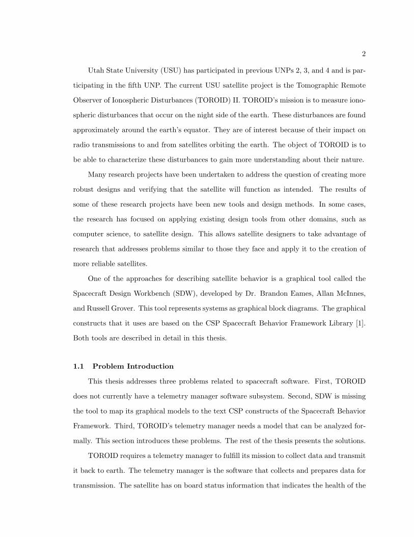
Utah State University (USU) has participated in previous UNPs 2, 3, and 4 and is par-
ticipating in the fifth UNP. The current USU satellite project is the Tomographic Remote
Observer of Ionospheric Disturbances (TOROID) II. TOROID’s mission is to measure iono-
spheric disturbances that occur on the night side of the earth. These disturbances are found
approximately around the earth’s equator. They are of interest because of their impact on
radio transmissions to and from satellites orbiting the earth. The object of TOROID is to
be able to characterize these disturbances to gain more understanding about their nature.
Many research projects have been undertaken to address the question of creating more
robust designs and verifying that the satellite will function as intended. The results of
some of these research projects have been new tools and design methods. In some cases,
the research has focused on applying existing design tools from other domains, such as
computer science, to satellite design. This allows satellite designers to take advantage of
research that addresses problems similar to those they face and apply it to the creation of
more reliable satellites.
One of the approaches for describing satellite behavior is a graphical tool called the
Spacecraft Design Workbench (SDW), developed by Dr. Brandon Eames, Allan McInnes,
and Russell Grover. This tool represents systems as graphical block diagrams. The graphical
constructs that it uses are based on the CSP Spacecraft Behavior Framework Library [1].
Both tools are described in detail in this thesis.
1.1 Problem Introduction
This thesis addresses three problems related to spacecraft software. First, TOROID
does not currently have a telemetry manager software subsystem. Second, SDW is missing
the tool to map its graphical models to the text CSP constructs of the Spacecraft Behavior
Framework. Third, TOROID’s telemetry manager needs a model that can be analyzed for-
mally. This section introduces these problems. The rest of the thesis presents the solutions.
TOROID requires a telemetry manager to fulfill its mission to collect data and transmit
it back to earth. The telemetry manager is the software that collects and prepares data for
transmission. The satellite has on board status information that indicates the health of the

3
system. It also collects science data. The telemetry data organizes the status information
and science data. The telemetry manager is necessary for managing all of this data.
The SDW tool does not have an interface to generate the equivalent CSP constructs in
the Spacecraft Behavior Framework from the graphical model. The CSP equivalent model
allows formal checks on the model to verify correctness. Without the CSP model, an SDW
model does not have support for model analysis. The model cannot be checked formally
without being translated first to CSP.
The telemetry manager is a complicated system made up of concurrent tasks and a
set of finite buffers. Showing that the system will run correctly requires a model that can
answer questions about the system. The model must represent aspects of the system so
that it can answer questions of how the system will work and if it will work as desired.
1.2 Thesis Overview and Layout
The results of research conducted with respect to modeling systems and software are
different tools that help designers describe these systems. These descriptions help designers
create system designs that are more concise and understandable. They also give an auto-
mated method of checking the system for correctness. Two of these tools are of particular
interest in this thesis. These tools are complimentary but lack support for each other;
this thesis presents the connecting thread between these tools. This thesis develops the
telemetry software subsystem for a small satellite and shows that it is possible to create an
analyzable model of it. This thesis also adds support for the SDW tool so it can generate
an analyzable CSP equivalent model. This thesis also extends the CSP libraries presented
by McInnes to allow a description of the satellite’s telemetry software system developed by
the USU Small Satellite Team.
The layout of this thesis is as follows. Chapter 2 gives discusses related research and
tool background. Chapter 3 gives some background on the USU Small Satellite TOROID
II project developed by a student team. The software system is described with particular
attention to the telemetry subsystem. Chapter 4 describes the graphical modeling tool
SDW and how this thesis connects it to the CSP libraries developed by McInnes. Chapter

4
5 discusses approaches to modeling the telemetry software for TOROID II and introduces
new constructs to help describe the software. It also discusses the analysis behind the new
constructs. Finally, Chapter 6 summarizes the work presented in this thesis.

5
Chapter 2
Related Work
Researchers have developed many different approaches to formal modeling, and have
applied the resulting approaches and tools to a diverse set of applications. A brief discussion
is presented here of some of the work that has been done and also some of the beginnings
of formal modeling.
2.1 Brief History of Process Algebra
A brief history of process algebras is given by Baeten [2]. Baeten describes a process
as the behavior of a system. Baeten uses the Merriam-Webster Dictionary definition of the
term process, which is defined as “something going on.” A process does not need to be
thought of as specific to a computer, indeed, it can be thought of in terms of a wide variety
of domains. Algebra in mathematics describes how numbers can be manipulated. Numbers
are manipulated by operators. There are rules for how these operators can be applied. A
process algebra describes “something going on” or the behavior of a system using a set of
rules that define operations that can take place. In a process algebra, the rules apply to
the events that are used to describe the process.
The advantage of being able to represent processes and having a set of rules defining
how the processes can be manipulated allows an exact analysis of how different processes will
interact. This detailed description provides a formal description of the processes because
they can be analyzed according to the set rules of the algebra.
The first process algebra was developed by Robin Milner. It is known as Calculus of
Communicating Systems (CCS). This first process algebra represents a significant step in
the way that concurrent systems could be represented and reasoned about.
Tony Hoare developed a different process algebra called Communicating Sequential
6
Processes (CSP). In CSP, Hoare does away with the idea of global variables. He instead
uses message passing to allow processes to communicate with each other. Milner later
adopts this idea as well for CCS.
Tool support has been created for both CCS and CSP. Concurrency Workbench sup-
ports CCS and a tool called Failures Divergence Refinement (FDR), which is the main
tool for analysis, supports the CSP algebra. Another tool that supports CSP is called the
Process Behavior Explorer (ProBE). ProBE allows a process to be traced through, so that
the user can explore a process one event at a time. It allows the user to explore the model
manually in a way that allows a better understanding of the process or processes.
The idea of a process algebra allows a precise representation of system components.
Tool support for these algebras allows rigorous analysis of the processes, this changes the
way that complex systems can be represented and checked for desirable behavior. Process
algebras provide an excellent method of creating a formal model of a system by representing
the system’s behavior in terms of processes. Process algebras also provide part of the base
for the research presented in this thesis. The algebra CSP is of particular interest because
it was the algebra of choice for the research that provides the underpinnings of this work,
both of which are discussed further later on in this thesis.
2.2 Graphical Modeling Language for Specifying Concurrency Based On CSP
CSP and its tools are not widely known or used by engineers. The textual language
is not a simple or intuitive method for design. This leaves the power of CSP to represent
concurrent systems largely unused in the commercial community. To give engineers tools
that are more intuitive, Hilderink introduces a graphical modeling language [3] to allow
engineers to specify concurrent systems. This graphical language is based on CSP. Hilderink
explains the language giving the graphical representation that corresponds to CSP concepts.
The focus in creating this language is to give the designer as much flexibility as possible to
represent a system using CSP concepts. Hilderink gives these concepts graphically so that
the designer is abstracted away from the actual textual language and does not require an
understanding of the mathematical basis of CSP.

7
Hilderink’s graphical CSP language extends CSP with the idea of process priority.
CSP does not inherently support the idea of priority. This allows the model to be analyzed
for priority inversion. Priority inversion occurs when a lower priority process executes
by blocking a higher priority process. Generally, priority inversion is caused by processes
of different priority sharing resources. This causes problems in embedded systems where
timing deadlines must be met.
This graphical language can also be used to detect deadlock. Deadlock occurs when
two or more processes are unable to continue execution due to waiting on a condition or
event that will never happen. Deadlock analysis is a key advantage that CSP offers and
Hilderink describes how this graphical language is able to aid in that analysis.
The graphical language allows designers to have the advantages of both modeling in
CSP and modeling with a graphical language. The CSP gives the analysis capability to the
designer while the graphical language gives a simpler interface for the user. In this thesis,
another approach is presented that gives designers these same advantages while keeping the
graphical front end abstracted further away from the details of CSP and utilizing design
techniques that are more similar to common graphical design languages.
2.3 Automatically Generated CSP Specifications
Two approaches are described by Scuglik [4] for generating CSP specifications of sys-
tems. The first translates a graphical flow type diagram into equivalent CSP. The diagram
syntax has an appearance similar to the actual CSP text that it represents. This means
that designs are not able to be created at a higher level of abstraction from the textual
CSP. A designer must still understand CSP, but the diagram does give a graphical repre-
sentation that is easier to use the the CSP code. The second approach Scuglik introduces
is a compiler that depends on a grammar to generate the CSP from an application’s source
code. Both approaches only use the basics of the actual CSP language which limits the
systems that they are able to describe. Both approaches are general and are not targeted
at any particular engineering domain.

8
2.4 Relationships between Common Graphical Representations in Systems
Engineering
Formal modeling relies on being able to capture a description of a system. Graphical
methods are generally easier for people to work with and understand. Long [5] details
different graphical methods of representing systems. Long defines two fundamental types
of graphical representations, functional flow and data flow. Functional flow block diagrams
(FFBDs) show a sequence of functions. A function may execute after its preceding function
has terminated, thus only the order the functions execute in is shown. Dataflow diagrams,
on the other hand, are concerned with data input to a function to determine when it can
execute. Control flow is not specified in a dataflow diagram. Long presents a combination of
functional and dataflow diagrams which capture both aspects of a system. He describes two
graphical modeling languages: Enhanced FFBD (EFFBD) and Behavior Diagrams (BD).
Both diagrams capture a combination of functional flow and data triggering.
Different views of a system allow designers to look at only one aspect at a time. This
hides unneeded details. This allows the designer to see only details of interest for a particular
view of the system. The EFFBDs and the BDs each provide different views of a system.
The functional flow of the system is captured by the EFFBDs while the data is captured
by the BDs.
The tools presented in this thesis are aimed at capturing the flow of data and the
function of the system. These tools and the information that they are able to capture are
discussed further on in this thesis.
2.5 Model-Based Engineering Design for Space Missions
Graphical tools allow a visual and generally easier method of capturing a design. Dif-
ferent approaches can be taken for capturing a design graphically. One graphical tool may
be a method of drawing a design by representing the flow of data or its behavior. Another
approach could be visualizing design trade-offs of the model graphically such as the tool
that Wall describes [6]. Design trade-offs are visualized by using a three-dimensional plot.
Each axis can represent a parameter that describes an element of the system. This allows

9
points to be plotted together and gives designers a graphical picture that shows trends and
patterns. This approach visually shows the designer the effects of different design trade-offs,
and allows the designer to pick the best set of parameters. It does not give the rigorous
verification techniques that the process algebra gives. The approach to graphical modeling
described in this thesis takes advantage of the rigorous verification of the process algebra
CSP.
2.6 Formal Modeling in a Commercial Setting: A Case Study
Chechik examines the application of formal modeling in a commercial setting [7].
Chechik discusses the hesitancy of commercial companies to adopt formal description tech-
niques. At least part of the reason given is that immediate benefits contrasted with long
term benefits are preferred. Chechik discusses the need for pilot studies in different en-
gineering domains that demonstrate the usefulness of applying formal methods. Chechik
further emphasizes that if these studies demonstrate the immediate benefits of applying
formal methods, commercial companies will find formal methods more enticing.
Chechik applied formal methods to a telephone service. This study shows how formal
modeling tools can benefit systems that are not considered critical. The system this case
study was applied to allows the creation of custom telephony applications. This could be a
voice menu that allows a user to select an option in response to a voice prompt. The tool
used to describe this system is the Specification and Description Language (SDL). SDL is
based on extended finite state machines.
Modeling the system allowed errors to be discovered in various phases of development.
Errors were discovered in the specifications as the models were created. The creation of
these models and removal of ambiguity in the specifications made it much easier to create
test cases. Errors were also discovered when creating test cases. The formal methods were
applied to this project in parallel with the normal development of the system. Full life cycle
comparisons were not made because desired statistics, such as the time to fix a bug, were
not tracked by the engineers doing the actual development. However, results observed from
this study suggest that development time can be positively impacted by the use of formal

10
tools. Development time impact depends on the domain and the availability of suitable
formal tools. As the author notes, other domains will likely use other formal language
specifications, some of which may not have existing tools available.
Tools for spacecraft design are emerging and two of these tools are discussed in detail
in this thesis. The work in this thesis extends these tools, described in Chapter 4, for
spacecraft design and enables users to more easily use these tools together.
2.7 Formal Analysis of a Space-Craft Controller Using SPIN
The usefulness and ability of formal methods to find errors and design bugs in real
working systems has been shown and described by Havelund et al. [8], which details the
case study of using Spin to check the correctness of a part of the software for a spacecraft
controller. The verification was performed on LISP code and was intended to model the
code and how its various threads interact with each other. Havelund says that the intent
was not to prove that the program was entirely correct, but improve the quality of the code
by capturing the main details in the model and checking for specific concurrent properties.
This is due to the fact that the model cannot capture the code in complete detail, but
is an abstraction that retains sufficient fidelity so as to permit the desired analyses. In
the end there were four errors detected by the model checker that were real errors in the
code. These errors were caused by particular sets of events. These event sequences were
obscure sets not likely to occur and so were not found by the developers during design or
testing. They were discovered by the formal model, however, and could be corrected during
the development phase. After the spacecraft was launched, an error in a part of the code
that was not modeled caused the system to deadlock in flight. Havelund claims that if the
particular part of the code that failed been modeled as well, the error would likely have
been caught during the design phase instead of during the actual mission. This case study
shows the value of checking a system rigorously with a formal model.
2.8 A Formal Approach to Specifying and Verifying Spacecraft Behavior
McInnes presented a set of CSP constructs which he developed to describe the system

11
behavior of small spacecraft [1]. These constructs have been developed specifically targeting
the description of system behavior of small spacecraft. Since these constructs are written
in CSP, each one can be analyzed using tools built to support CSP. A designer can create a
model of a system in CSP and also a CSP system specification. Then, using the CSP tools
available, check that the system meets the specifications. This thesis uses the work done
by McInnes [1] as a foundation for further investigation.
2.9 The Generic Modeling Environment
The Generic Modeling Environment (GME) is a highly customizable graphical model-
ing tool that lets the user create a domain specific modeling environment. The user creates
the environment by specifying the types of objects it can contain and how they can be
connected or related to each other. The environment rules that specify the types of objects
and how they can be connected or related is captured in the environment’s meta-model. At
a high level, GME allows the user to create a customized block diagram tool, defining the
blocks and the lines connecting the blocks.
GME also provides an application programmer interface (API) that gives functions and
routines that can read a model created in the environment. A program can use this API
to interpret the model. This interpretation allows a model to be analyzed automatically in
a meaningful way. For example, an interpreter may search the model and give a summary
of what components the model contains. Another example would be an interpreter that
determines an optimal solution based on the model.
The meta-model in GME contains all of the information necessary to specify how a
model can be created. The meta-model is specified using a graphical specification language
similar to UML. All meta-models are composed of several building blocks and relation-
ships between these blocks. The main meta-model building blocks and their relations are
described here. There are other objects that make up a meta-model. However, the ob-
jects described below are those that are applicable to the SDW meta-model. The main
components of a meta-model are:
12
• atoms,
• models,
• connections,
• attributes,
• inheritance,
• first class objects (FCO).
Atoms are the fundamental blocks of a meta-model. Atoms are the basic means of
representing abstractions of real system components. Since atoms are the fundamental
basic block, they cannot contain other objects. They can, however, be contained in other
objects, they can also be related to other objects by means of one or more connections.
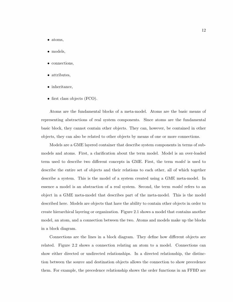
Models are a GME layered container that describe system components in terms of sub-
models and atoms. First, a clarification about the term model. Model is an over-loaded
term used to describe two different concepts in GME. First, the term model is used to
describe the entire set of objects and their relations to each other, all of which together
describe a system. This is the model of a system created using a GME meta-model. In
essence a model is an abstraction of a real system. Second, the term model refers to an
object in a GME meta-model that describes part of the meta-model. This is the model
described here. Models are objects that have the ability to contain other objects in order to
create hierarchical layering or organization. Figure 2.1 shows a model that contains another
model, an atom, and a connection between the two. Atoms and models make up the blocks
in a block diagram.
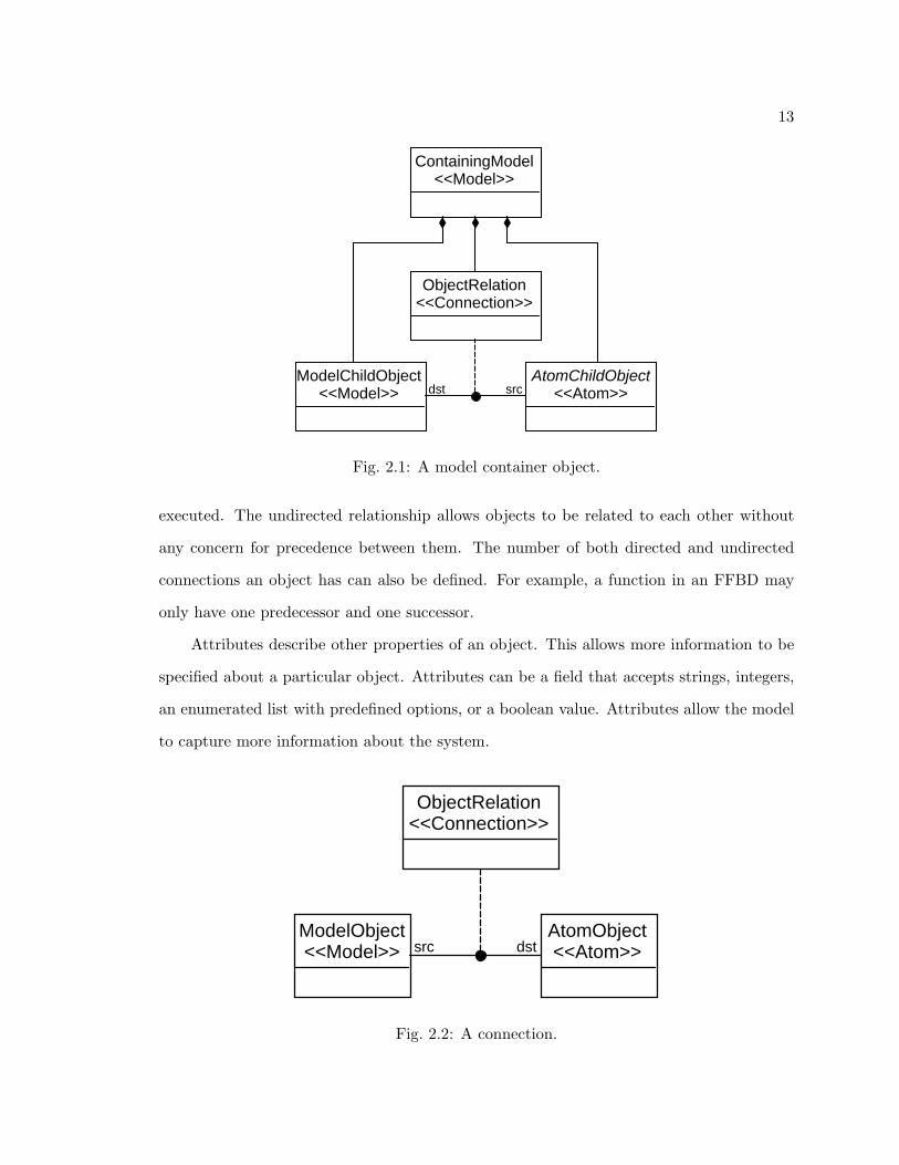
Connections are the lines in a block diagram. They define how different objects are
related. Figure 2.2 shows a connection relating an atom to a model. Connections can
show either directed or undirected relationships. In a directed relationship, the distinc-
tion between the source and destination objects allows the connection to show precedence
them. For example, the precedence relationship shows the order functions in an FFBD are
13
ContainingModel<<Model>>
ModelChildObject<<Model>>
AtomChildObject<<Atom>>
ObjectRelation<<Connection>>
dst src
Fig. 2.1: A model container object.
executed. The undirected relationship allows objects to be related to each other without
any concern for precedence between them. The number of both directed and undirected
connections an object has can also be defined. For example, a function in an FFBD may
only have one predecessor and one successor.
Attributes describe other properties of an object. This allows more information to be
specified about a particular object. Attributes can be a field that accepts strings, integers,
an enumerated list with predefined options, or a boolean value. Attributes allow the model
to capture more information about the system.
ObjectRelation<<Connection>>
ModelObject<<Model>>
AtomObject<<Atom>>dstsrc
Fig. 2.2: A connection.

14
Inheritance relations allow objects to share common characteristics. Objects may even
be identical as far as connections and attributes are concerned, but represent distinctly
different objects in the model. To make the meta-model easier to construct and also cleaner
to read, objects may inherit from a common parent. The object that inherits from its
parent will have all of its parent’s characteristics. An object may inherit from more that
one parent object.
First class objects (FCOs) serve as parent objects for both models and atoms. An
object can only inherit from other objects which have characteristics the child object can
also have. For example, an atom cannot inherit from a model because it cannot contain
other objects like the model can. Likewise the model cannot inherit from an atom. However,
there are certain characteristics that atoms and models may have in common. A common
object is needed that both types of objects can inherit from, this is accomplished with a
FCO. Observe in fig. 2.3 how the parent FCO has both an atom and a model inheriting
from it. FCOs are abstract objects and therefore cannot be instantiated in a model. If an
atom is to inherit from an FCO, the FCO cannot have any characteristics that an atom
cannot have. This means an FCO cannot be defined to contain any type of object when an
atom inherits from it.
All of these objects are used to make a meta-model and are available in GME’s meta-
model paradigm. A paradigm is what configures GME for a particular modeling envi-
ronment. When a meta-model is complete, it is translated into its own paradigm. This
new paradigm configures GME to support models conforming to the rules defined in the
paradigm’s meta-model. Models can then be visualized and edited in GME using the
paradigm. GME provides the environment for the tool described in Chapter 4, which has
been accepted for publication [9].

15
ModelChildObject<<Model>>
ParentObject<<FCO>>
AtomChildObject<<Atom>>
Fig. 2.3: FCO inheritance.

16
Chapter 3
TOROID II
An understanding of the TOROID II satellite system forms the base of the discussion
of the modeling tools and techniques in the rest of this thesis. This chapter describes the
TOROID II satellite at a systems level and discusses the software in more detail since the
software implements most of the system behavior. An understanding of the satellite’s system
behavior establishes an understanding of what the models are able to capture. The satellite
was still under development at the time this thesis was written, and as it matures and
subsystems are refined, new information may be revealed that may require a re-examination
to ensure a consistent design. The most complete description of the TOROID software can
be found in the report TOROID Software Subsystem [10]. This chapter describes the
TOROID subsystems and then details the telemetry subsystem giving the design that has
been refined during the development and functional testing that it has gone through.
3.1 TOROID II Concept of Operations
As introduced in Chapter 1, the mission of TOROID II is to take measurements of the
ionosphere. These measurements are to be taken on the night side of the earth over the
equatorial region. As it passes over this region, samples of light will be taken in the extreme
ultra violet spectrum. When the satellite passes over Logan, Utah, the sampled data will
be transmitted to the ground station. All of these actions must be incorporated into the
satellites behavior. The following section describes the subsystems designed to execute the
mission.
3.2 TOROID II Subsystems
TOROID II is a nano-satellite, having a mass of approximately 50 Kg. and is com-

17
posed of several subsystems. These subsystems are consistent with those typically found on
satellites but are briefly described here to provide background and also facilitate a definition
of the scope of this research. TOROID’s primary subsystem’s include:
• structure,
• command and data handling (C&DH),
• communications,
• software,
• power,
• attitude determination and control (ADC),
• mechanisms,
• harness,
• thermal,
• science.
The structure is purely a mechanical subsystem. The shape of the structure determines
the behavior of the ADC system. In this work the ADC system is assumed to function
correctly and its impact is not captured in the type of modeling undertaken by this research.
The thermal subsystem has properties that have an effect on the behavior of the satellite.
Heat dissipation is a key aspect of satellite design that must be considered. The operational
modes of the satellite use different electronics, these electronics generate a certain amount
of heat that must be dissipated. Neglecting the thermal design can leave the electronics
overheating which can lead to mission degradation and possible failure. Despite the impact
that the thermal design of the satellite can have on behavior, it is not included in the scope
of this research.

18
3.2.1 Command and Data Handling
The Command and Data Handling subsystem includes the electronics of the satel-
lite. Figure 3.1 shows the architecture of TOROID’s electronics. The C&DH includes the
following components:
• backplane,
• trigger board,
• camera board,
• telemetry board,
• CPU board,
• IO board,
• motor board,
• science board,
• power boards one, two, and three.
Detailed information on many of these boards can be found in The Design of the
Command and Data Handling Sub-system Used by the Ionospheric Observation Nano-
Satellite Formation [11]. These boards allow the system to gather data from its sensors and
make decisions based on those readings. They also facilitate the receipt and processing of
commands which are sent by the ground station. The space environment, in which these
electronics will be deployed, is quite different from the terrestrial computing environment,
offering a unique set of challenges that must be taken into consideration when designing
computer hardware. The primary consideration that must be addressed is radiation.
Single event upsets (SEUs) can cause sporadic changes to digital signal levels and stored
bit values in typical digital electronics. More problematic than SEUs are singe event latch
ups (SELs). A SEL is basically a short circuit caused by radiation, the resulting current can

19
quickly overheat the electronics and cause permanent damage to the hardware. Just one
SEL has the potential to destroy hardware that would most likely result in mission failure.
The solution for SELs that has been taken is to monitor the current on each of the boards.
If the current gets too high, the board is power cycled. This resets the circuit that was
latched, eliminating the short, and prevents it from being damaged. Figure 3.2 shows the
design of the C&DH with the power monitoring system in place. Clearly this design can
impact the behavior of the entire satellite, since at any time any of the individual boards
or even the entire C&DH subsystem can be reset.
3.2.2 Communications
The ground crew must be able to communicate with the satellite as it orbits around
the earth. From a high level, this includes two major parts, the ground station and the
communication system onboard the satellite. The ground station includes all of the com-
puters, radios, antennas, tracking system, and other equipment that allows signals to be
sent from earth to the satellite and also receive signals from the satellite. Using the ground
station, commands can be transmitted to the satellite. The ground station is also able to
capture the data that is downlinked from the satellite.
The satellite has two radios. The first radio operates on the ultra high frequency (UHF)
range and is a half duplex communication link with the ground station. The second radio,
the S-band radio, is used for downlinking only. It transmits science data collected by the
satellite to the ground station.
3.2.3 Software
The heart of the satellite’s behavior is the software subsystem. The software is able to
run on the C&DH system to provide the decision making algorithms that ultimately will
determine how the satellite interacts with its environment. Software overlaps almost all of
the other subsystems. The software architecture has been constantly updated and modified
during the lifetime of the nano-satellite program.

20
Hitachi SH3 7709
Microprocessor
CPU Board
PROM
Flash
SRAM
Voting
Logic
FPGA Watchdog
Timer
FPGA
SPI BusOne Wire
Bus
Memory Subsystem
Motor BoardPower Board
Camera Board
Flash
FPGA
Telemetry Board
FPGA
Digital
I/O
Analog
I/O
Digital I/O
A/D Converters
I/O Interfaces
I/O Board
RS422
RS232
Serial Interfaces
RS232OTP
Science Board Temperature
Sensors
TNC
SRAMFlash
S-Band
Transmitter
UHF
Transceiver
Trigger Board
Fig. 3.1: TOROID II C&DH design.

21
Power
Board
CPU Board
Digital I/O Analog Inputs
Analog InputsDigital I/O
Current
Monitor
Current
Monitor
I/O Board
MOSFET
Switch
Current
Monitor
Motor Board
MOSFET
Switch
Current
Monitor
Science Board
MOSFET
Switch
Current
Monitor
Telemetry Board
MOSFET
Switch
Current
Monitor
Camera Board
MOSFET
Switch
Current
Monitor
Digital Control Signals
Interrupt Signal
Satellite Power
Fig. 3.2: SEL recovery scheme.

22
Figure 3.3 shows the software architecture of the TOROID satellite divided into sub-
system managers and memory blocks. The managers are sets of concurrent tasks that
have continuous looping execution. The software is divided into the following subsystem
managers:
• UHF manager,
• power & temperature manager,
• science manager,
• system state recorder,
• telemetry manager,
• ADCS manager,
• deadlock detection watchdog.
Each manager is an independent process or set of processes implemented in software.
These managers are all executed on the main system CPU and are able to access the other
parts of the system as required by their functionality. Their execution is handled by a real-
time operating system. In addition to the different managers, there are designated blocks
of memory that allow storage of data that have global significance. These memory blocks
are:
• global status structure,
• system log,
• system state.
The managers need to be able to share information with each other. A simple shared
memory structure has been set up, called the global status structure (GSS), that facilitates
data sharing. The GSS is simply a structure that has separate partitions for each of the

23
GSS
Sys Log
Sys State
UHF Manager
ADCS Manager Power & Temp Manager
Science ManagerTelemetry Manager
System State Recorder
Deadlock Detection Watchdog
Event Log Manager
Execution
Data flow
Fig. 3.3: Software architecture.

24
managers, allowing them to store shared variables. As needed, read access is granted to
other partitions to permit sharing. Each partition is protected by semaphores to guarantee
mutual exclusion between manager accesses.
The system log allows the system to write events of interest to a persistent storage
location that can be later downlinked to the ground station for analysis. This is designed
to provide engineers on the ground with valuable information to determine if the spacecraft
is functioning correctly, and if not, to diagnose potential causes of unexpected behavior.
The system state allows for storage of the current operational state of the satellite in
persistent memory. The system state is composed of the GSS and also data specific to
the software managers. This data is normally located in volatile memory which will be
lost when the system is reset. Storing the system state in non-volatile memory enables the
satellite system to be restored to an operational state in the event of a system reset.
UHF Manager
The UHF manager is the software responsible for handling communication to and from
the ground station. It listens to the terminal node controller (TNC) which processes signals
sent and received to and from the ground station over the UHF radio. When a signal is sent
from the ground station to the satellite, the TNC decodes, digitizes, and buffers the signal.
This allows the UHF manager to read the command or data sent. The UHF manager is
responsible for processing and executing commands from the ground station. This allows
the ground station crew the capability of modifying the spacecraft state by controlling the
instruments and devices on the satellite remotely. This also allows the ground station crew
to request status data from the satellite.
Using the UHF manager the ground station crew is able to send the command to
initiate a downlink of the science data that has been collected over the S-band transmitter.
The UHF manager is also responsible for making sure that only commands sent from the
ground crew are processed so that control of the satellite is not lost to a third party and so
that no third party can inadvertently send commands that could have negative affects on
the operation of our satellite.

25
Power and Temperature Manager
Power is a critical aspect for the success of any spacecraft. The power and temper-
ature manager monitors the power and temperature of the satellite. It is responsible for
determining when load shedding needs to be done so that the power level does not drop to
dangerously low levels that could jeopardize the survival of the satellite. It is also responsi-
ble for allowing tasks and functions to continue once the power level has reached a nominal
level. It also monitors the temperature of the satellite and updates the GSS. Proper tem-
perature plays a vital role in the correct functioning of the onboard batteries and must be
monitored to ensure proper operating temperature.
Science Manager
The science manager is responsible for running the science instruments and making the
data read from them available to the telemetry manager. The main science instrument is
called the photometer. The photometer is able to take light measurements needed for the
science mission of TOROID. The science manager ensures that the photometer is operated
correctly and at the times specified by the ground station.
System State Recorder
The system state recorder is responsible for periodically saving the system state to
non-volatile memory. This provides a snapshot of the current satellite’s state so that in the
case of an unexpected system reboot the satellite can be brought back on line as quickly as
possible. This helps protect against data loss and mission down time.
There are several reasons the system may reboot unexpectedly. A reboot may be
required to protect the CPU from a radiation latchup event. Unexpected behavior could
cause the system to deadlock. In a deadlocked state, no code is able to execute due to
resource conflicts. This is basically when each process is waiting for another process to
release a resource but none of the processes are able to access all of the resources needed to
complete execution. This causes an endless wait state known as deadlock. There is a watch
dog timer that will reboot the system after a long period of inactivity. With the ability

26
the save a copy of the system state in non-volatile memory, the effects of these unexpected
system reboot events can be minimized.
Telemetry Manager
The telemetry manager is responsible for gathering, formating, and storing data to
non-volatile memory to await downlink. The first task of gathering is designed to collect
the telemetry, or housekeeping, data from the GSS, image data from the cameras, and
experiment data from the science instruments. The data is then formated and stored
in preparation to be transmitted to the ground station. The telemetry manager will be
discussed in detail later in this chapter.
ADCS Manager
The ADCS (attitude determination and control system) manager is responsible for
control of the satellite’s attitude. There are two sources of attitude information available
to the ADCS manager, magnetometer coordinate readings and camera image data. The
magnetometer uses the earth’s magnetic field to give three axis coordinate readings. The
cameras capture images that show the horizon of the earth, this shows how the satellite
is oriented in relation to earth. The ADCS manager reads the magnetometer and image
data to determine the tumble rate and attitude of the satellite. To orient the satellite
relative to earth, there are three magnetic coils, called torquer coils, that will push against
the earth’s magnetic field which allows the satellite to orient itself. Once the satellite is
oriented correctly, it is able to maintain a steady attitude through the torquer coils and
also a momentum wheel. The momentum wheel is a motor that spins a weight, creating a
momentum bias that stabilizes the satellite.
There are two basic modes of operation of the satellite, science mode and station
keeping mode. Station keeping allows the satellite to communicate to the ground station
via the onboard radios. Station keeping mode is a relatively stable state that keeps the
satellite oriented with the bottom of the satellite pointing to earth. Science mode is a
more stable attitude that allows meaningful science data to be collected. Control for both

27
the science and the station keeping satellite modes is done by the ADCS manager. One
challenge for TOROID II is that the science instrument has a spinning sensor mounted to
the side of the satellite. The spinning motion of the sensor creates a momentum bias that
must be taken into account in order to maintain the satellite in the desired attitude. Since
the spinning motion of the science instrument has an impact on the attitude control, the
ADCS manager must be able to maintain correct attitude of the satellite whether or not
the science instrument is spinning.
Deadlock Detection Watchdog
Unforeseen behavior of the software system could lead to a deadlock state, described
earlier, where none of the software processes are able to execute. If the system deadlocks
without a way to detect and recover from it, the mission would fail, since the software han-
dling the satellite’s communication system would also be unable to respond to commands
sent by the ground station making communication with the satellite impossible. The ground
crew would be left with no means of understanding what went wrong, nor any ability to
correct the problem. For these reasons the software system contains a watchdog timer that
detects when no processes are running on the CPU. After 15 seconds, if no activity is de-
tected, the system is rebooted. This watchdog provides a safeguard against the unexpected
deadlocks in the software system.
3.3 Telemetry Manager Design
The telemetry manager is responsible for the collection, formatting, and storage of all
data downlinked to the ground station. Prior to this work, TOROID had no viable telemetry
manager system. An initial architecture was outlined by students working on the software.
However, the outlined architecture could not be fully implemented to meet the required
functionality. The telemetry manager software described in this section meets the needs of
the TOROID mission. At the time this manager was written, specific details regarding the
amount of science data were not available. The architecture presented is flexible and easily
adaptable to any data requirements that are determined by the TOROID team.

28
This section describes how the telemetry manager uses a set of periodic tasks, and
buffers to accomplish data collection and formating. It also describes how the data is
gathered from multiple sources using a set of buffers. It shows how tasks are controlled to
have consistent periodic behavior. It also describes the relationship between the telemetry
manager software and the telemetry board hardware.
3.3.1 Task Control
The telemetry manager tasks are run at specific periods. These periods are enforced
through a combination of semaphores and timers.
A semaphore is a variable that maintains its correctness when multiple processes are
trying to read or write to it at the same time. Reads and writes to a semaphore are atomic
operations. An atomic operation cannot be subdivided. A single statement in a high-level
programming language is divided into several assembly instructions. These instructions
can be interleaved with instructions from another task. If both tasks are attempting to
access the same data, the interleaved instructions can cause the data to become corrupted.
When a semaphore is accessed, it is done with atomic statements that cannot be divided
into multiple instructions. This means that the semaphore data accessed by an atomic
statement is not corrupted due to conflicting interleaved instructions.
Binary semaphores have two values, one or zero. They are used to control access to
shared data and to synchronize processes. The semaphore used to control a task’s period
provides synchronization between the task and its timer. The task executes in a loop.
Before it can repeat the loop it must synchronize with its timer. To synchronize with its
timer, the task tries to decrement its semaphore. If the semaphore is zero, the task must
wait until the semaphore has been set to one. The task is notified when this happens. At
this point the task continues executing its loop until it hits the semaphore again.
A timer allows a function to be associated with a time delay. In VxWorks, the timer is
maintained as a part of the system clock interrupt service routine (ISR). When the timer
expires, the function associated with it is executed at the priority of an ISR [12]. For this
reason the function associated with the timer should be a small, short function. To create

29
a periodic task, the function associated with the timer does two things. First, it releases
the semaphore for the task controls. Second, it restarts its timer. This process repeats as
long as the task is running.
A semaphore combined with a periodic timer creates a way to run a task at a given
periodic rate. The steps for the timer function and the task are given below.
Timer:
1. Wait specified time,
2. Set semaphore to one,
3. Reset timer to task’s period,
4. Repeat.
Periodic Task:
1. Execute task operations,
2. Set semaphore to zero, block until it is available,
3. Repeat.
Each periodic task has this behavior, using the associated timer and semaphore to
control its period.
3.3.2 Telemetry Data Formating
All of the data that the telemetry manager collects is formated into a matrix prior to
transmission. The matrix is designated as the pulse code modulation (PCM) matrix. This
is in reference to the encoding used to transmit the data over the S-band transmitter. The
PCM matrix, as far as the telemetry manager is concerned, is a two-dimensional array. The
array is composed of sub-frames and pages. There are 64 bytes in a sub-frame and 256
sub-frames in a page. This gives one page a total size of 16,384 bytes.
The data is distributed between the different sources as shown in fig. 3.4. There are
eight different data groups. Each group is given with the number of bytes dedicated to it

30
in each sub-frame. The first group is a set of sync words. The sync words indicate the
beginning of a sub-frame. The second group is the sub-frame ID (SFID). The third group
is the housekeeping (HK) data. HK data describes the physical state of the satellite. This
includes voltages, current, temperature, and battery power levels, etc. All of the HK data
is stored in the GSS. The fourth group is image data. The images are taken by the onboard
cameras. The fifth group is a status byte. This status byte is needed more often than the
HK group will allow, so it is set as its own group. The sixth group is science data from the
direct current probe (DCP). The seventh group is science data from the impedance probe
(IP). The eight group is science data from the photometer (PHO). The photometer is the
main science instrument on TOROID.
3.3.3 Telemetry Manager Architecture
The telemetry manager is a continuously looping periodic process. The main telemetry
manager is made up of three loops, as shown in fig. 3.5. The inner loop collects data for
one sub-frame. Data is collected in the order defined by the PCM matrix. This is how the
data is formated. The inner loop is repeated 256 times for each page. The middle loop
collects data for eight pages. When eight pages have been collected, the buffer is written
to flash by a concurrently running task. The main telemetry manager continues collecting
data with a second buffer while the first buffer is written to flash. These alternating buffers
are designated as ping and pong. All of the buffers that are used in the telemetry manager
are first in first out (FIFO) ordered buffers.
Sync Sub-Frame ID HK Img TQR DCP IP PHO (2 bytes) (1 byte) (1 byte) (4 bytes) (1 byte) (2 bytes) (6 bytes) (47 bytes)
Sync 0 HK img TQR DCP IP PHOSync 1 HK img TQR DCP IP PHO
… … … … … … … …Sync 254 HK img TQR DCP IP PHOSync 255 HK img TQR DCP IP PHO
Fig. 3.4: PCM page format.

31
Pick buffer(ping or pong)
For 8 Pages
For 256 sub frames (build sub frame)
8 pa
ge b
uffe
r
Synch word2 bytes
Sub-frame ID (SFID)1 byte
Name: HKType: Housekeeping class
1 byte
Name: imgType: FIFO class
Image data, 4 bytes
Name: readTQR Type: function
not implemented, 1 byte
Name: sc12 Type: FIFO class
DC probe data, 2 bytes
Name: sc34, sc56, sc78 Type: FIFO class
Impedance probe data6 bytes
Name: pho Type: FIFO classPhotometer data
47 bytes
Data Sources
Name: GSSType: Structure
Name: sampleImageType: FIFO class
Name: GSSType: Structure
Name: sampleDCP()Type: Process
Name: sampleIP() Type: Process
Name: samplePHO()Type: Process
Telemetry Manager loop
Data request
Data request
Fig. 3.5: Telemetry manager flow.

32
Data is stored to the eight page buffer in the order defined by the PCM matrix in fig.
3.4. This order can also be seen in fig. 3.5. The sync words are constants and are the same
for every sub-frame. The SFID is a number tracked by the inner most loop. The SFID
repeats itself for each PCM page.
The housekeeping class is a C++ class that manages gathering and storing house-
keeping data. Housekeeping data is all stored in the GSS. Many of the housekeeping data
values are multi-byte, but each sub-frame stores only one housekeeping byte. To manage
this problem, the multi-byte values are read from the GSS and stored by the housekeeping
class. They are then read from the housekeeping class byte by byte and stored in the PCM
page. The housekeeping class interfaces the telemetry manager with the GSS and handles
all housekeeping data gathering. One set of housekeeping data is collected for each page.
Images are stored by a FIFO class that buffers the image data. An image is 512 x 512
bytes, or 256 KB. Images are stored to the PCM page at rate of four bytes per sub-frame.
This means 65536 frames, or 256 pages, are required to store one image.
The TQR byte is a status byte for the ADCS. It is needed more than once per page, to
accommodate this it is in its own group. It is a data value stored in the GSS and accessed
by a function. There is no need to buffer this data.
The DC probe, impedance probe, and photometer data make up the bulk of the PCM
page. They are the science instruments gathering data for the TOROID mission. Data is
handled the same way for each of these instruments. Data sampled from each instrument
is stored in its own FIFO class buffer. The data is then read by the telemetry manager at
the correct rate and stored in the sub-frames. The FIFO buffers allow data to be gathered
by the science instrument at one rate and stored in the PCM page at different rate.
3.3.4 The Telemetry Board
The telemetry board is designed to store data and send it to the S-band transmitter
for transmission to the ground station. It is part of the C&DH subsystem shown in fig. 3.1.
The telemetry board has onboard flash memory that stores telemetry data. The CPU has
a direct connection to the telemetry board flash. The CPU writes data to the flash memory

33
through this connection. When the ground station commands the satellite to transmit the
stored data, the telemetry board disables the CPU’s connection to the flash memory. The
data is then transmitted to the ground station through the S-band transmitter. When the
transmission is complete, the flash memory is erased. The telemetry board then re-enables
the CPU’s connection to the flash memory.
The CPU and telemetry board function independently during transmission of the
telemetry data. The telemetry manager executes on the system CPU. This decouples the
telemetry manager and the telemetry board. The telemetry manager is able to continue
collecting and formatting data while the telemetry board transmits the contents of its flash
memory. The telemetry manager continues to collect data until both the ping and pong
buffers are full. In the worst case scenario for buffer space, the telemetry flash is taken off
of the memory and data buses just before one of the buffers is written. In this case, the
telemetry manager continues collecting data for the time it takes to fill one buffer. The
time to downlink is less than the time required by the telemetry manager to fill one buffer,
this allows the telemetry manager to continuously sample data even while data is being
downlinked to the ground station.
3.4 Conclusion
The TOROID II satellite is composed of many subsystems that depend on and interact
with each other to complete the spacecraft’s mission. Given the environment in which
the satellite must operate and the limited access the operator has to the system, it is
vital that these interactions take place as planned in order that the mission is successful.
The complexity of these interactions makes it difficult for typical trial testing to uncover
problems in the behavior of the software. Modeling methods can be applied to the software
system to help check its behavior in a thorough, systematic manner. The following chapters
explore a specific modeling tool and its application to TOROID II.

34
Chapter 4
The Spacecraft Design Workbench
Formal methods give powerful ways for describing and verifying behavior of complex
systems and the ability to perform rigorous checks and analysis of the system model. Space-
craft especially benefit from such analysis because of the nature of their typical missions
and the harsh environment in which they operate. Correcting mistakes on a spacecraft in
orbit or on a deep space mission is extremely expensive and time consuming. Therefore,
the benefits that can be realized by such projects by using formal methods are potentially
much higher than other engineering projects.
The difficulty most engineers face in using formal methods is that it takes a great deal
of study and experience to effectively use them. To mitigate this problem, an approach has
been taken to design a tool to facilitate the use of formal methods by giving an intuitive
front end for users to describe system behavior [13]. The resulting tool is the Spacecraft
Design Workbench (SDW). This chapter describes the tool [9], and the additions made by
this research.
The purpose of SDW is to give the user a GUI front end that uses design methods
familiar to most engineers. This gives a tool that is easier to learn than CSP and its
supporting tools. SDW uses a graphical modeling tool that enables engineers to create
a graphical model as a type of block diagram. Once the model has been created, it can
be translated to CSP [14, 15], which has tool support for rigorous analysis. Once CSP is
generated from the model, the commercial tool FDR2 (by Formal Systems) can be used to
perform analysis on the model. SDW is based on several different tools and semantics that
will be discussed in the following sections.

35
4.1 Functional Flow Block Diagrams
There are many different ways to describe the behavior of a system. A common method
involves a set of functions that are organized together into a graph to show the order in which
they should be executed. This graph is called a functional flow block diagram (FFBD) [16].
An example of an FFBD is shown in fig. 4.1. The basic block in an FFBD is a function.
A function is simply a block that represents something that should be performed or code
that is to be executed. The syntax of how functions can be put together as a functional
flow block diagram to form a system is simple and intuitive to understand. Functions can
be organized in five different ways:
• sequence,
• concurrency,
• selection,
• choice,
• iteration.
Sequence shows the order in which the functions will execute. As seen in fig. 4.1,
function 1 precedes function 2. In preceding function 2, function 1 must completely finish
before function 2 can begin.
Concurrency shows two or more paths that have the potential to run simultaneously.
In fig. 4.2 there are n paths to be taken, the concurrency structure will not be finished until
all paths have completed, at that point the FFBD can continue. Note that the functions
are not guaranteed to be executed simultaneously, but the possibility exists. Thus, the
functions in a concurrent block can be mapped to a single core or multi-core processor.
Function 1 Function 2 Function n
Fig. 4.1: FFBD sequence.

36
n
Fig. 4.2: FFBD concurrency.
Selection presents two or more paths that can be executed, only one path will be chosen,
however. In fig. 4.3, there are n different possible execution paths. It is important to note
that only one of these paths can be taken. There is no condition on any of the paths and
each is assumed to be equivalent in function so it does not matter which path is selected.
Choice allows a condition to be specified and one of two paths taken depending on
the outcome of the condition. This is similar to an if else clause in the C programming
language. Figure 4.4 shows a choice construct that will execute function 1 if the condition
is true and function 2 if the condition is false.
Iteration allows certain functions to be executed repeatedly depending on an iteration
condition. In C this is similar to a do while loop because the function is executed once before
the loop condition is evaluated. Figure 4.5 shows how the iteration construct is made using
the choice function as the loop condition to control when the loop terminates execution.
4.2 Data Flow Diagrams
The FFBD can specify when a function should be executed relative to other functions.
The function itself is described by another type of diagram known as a data flow diagram
(DFD). McInnes describes a function as a mapping from a set of inputs to a set of outputs.
This means that every input symbol is associated with an output symbol, in other words it
is mapped to that output symbol. This is essentially what a DFD function does, it maps

37
n
Fig. 4.3: FFBD selection.
Choice
Function 1True
FalseFunction 2
Fig. 4.4: FFBD choice.
ChoiceFunction 1
Done
Not done
Fig. 4.5: FFBD iteration.

38
an input symbol to a specific output symbol. These functions are always ready to fire, so
anytime an input is provided, the output is triggered. Figure 4.6 shows a function f(x) that
has a one-to-one mapping from the domain to the range. The mapping does not need to be
one-to-one, however. Observe the function g(x) in fig. 4.7. In this scenario, both a and b
map to unique values, but c and d map to the same value. The DFD function simply maps
a domain value onto its corresponding range value.
Since the DFD functions have no way of knowing when to execute and also have no
way to control their own execution, a method of execution control is needed. Execution
control is achieved by integrating DFDs with FFBDs. The fundamental unit of an FFBD
is a function. If we use a DFD as the FFBD’s function, the FFBD controls the execution
of the DFD.
The CSP basis for describing DFDs and FFBDs is described in A Formal Approach
to Specifying and Verifying Spacecraft Behavior [1]. The CSP processes make up the an-
alyzable base that allows model checking on a system. The goal of SDW is to translate a
graphically specified system of DFDs and FFBDs into their equivalent CSP processes.
4.3 Constraints
In CSP it is common practice to create a process that can be used to modify the behav-
ior of a system process without actually modifying the system itself. This type of process
is known as a constraint process. The constraint process is applied to the system by having
key system events in common that require the system to synchronize with. Constraints are
useful to help describe an entire system by using it to modify the way that different parts
⎪⎪⎭
⎪⎪⎬
⎫
⎪⎪⎩
⎪⎪⎨
⎧
⇒
⎪⎪⎭
⎪⎪⎬
⎫
⎪⎪⎩
⎪⎪⎨
⎧
=
δλβα
dcba
xf )(
Fig. 4.6: DFD function f(x).

39
⎪⎪⎭
⎪⎪⎬
⎫
⎪⎪⎩
⎪⎪⎨
⎧
=
dcba
xg )(
⎪⎭
⎪⎬
⎫
⎪⎩
⎪⎨
⎧
δ
αß
Fig. 4.7: DFD function g(x).
of the system behave. Constraints give descriptive power that allows the user to clearly
specify the desire behavior.
To illustrate the usefulness and applicability of constraints, consider a problem that
has been used to compare systems engineering tools and techniques, the traffic light prob-
lem described in The Design-Methods Comparison Project [17] by using different design
techniques. Consider a simple traffic light that cycles through its three states and does
not consider current traffic conditions but executes a preprogrammed execution sequence
of turning the light red, then green, then yellow, and then repeating itself.
An intersection of two roads, Oak Street and Elm Street is controlled in each direction
by this simple light. Each road has a light that follows the sequence red, green, yellow. This
translates into a single CSP process. However, if these systems are run together, there is no
synchronizing or safety enforced and each light would run independently of the other. With
no synchronization between the two lights, they could easily overlap and non-sensical and
dangerous combinations could be reached such as both street lights turning red or green at
the same time.
Now, consider the case in which the Elm Street system could have its light turn green
only after Oak Street’s light had turned red. The same for Oak Street’s green light, it can
only turn green after Elm Street turns red. In effect, the system needs to have its green
light (and yellow for a complete description) disabled from the time that it turns red, to
the time that the other system light turns red. This relationship between these systems can
be captured using one of two constraints that will be discussed next.
The work done by McInnes to describe satellite behavior using CSP processes includes

40
a method of adding constraints to the system. Two of the constraints that he included in his
CSP framework are called between and outside constraints. These constraint processes were
first introduced in The Theory and Practice of Concurrency [14]. The high-level concept is
intuitive to understand. Each constraint is a process and is made up of three main sets of
events:
• enable,
• disable,
• enabled.
The easiest way to understand these event sets is graphically, both between and outside
constraints are shown in fig. 4.8.
4.3.1 Between Constraint
The between constraint has an event, enable, that acts as a trigger. Once an event
from the enable set has occurred, events in the enabled set are allowed to execute. The
enabled events can continue to execute until an event from the disable event set occurs.
In short, the enable event acts like turning a switch on to allow enabled events, and the
disable event acts like turning the switch off. Events in the enabled set can occur between
the enable and disable events, hence the designation between constraint.
enabled events
enable event disable event
enabled events
enable eventdisable event
enabled events
between
outside
Fig. 4.8: Between and outside constraints.

41
For the traffic light example, using a between constraint is intuitive since when the Oak
Street light turns red, the Elm Street light should not be able to turn green until the Elm
Street light has turned red, at that point it cannot turn green until the Oak Street light
turns red again. As illustrated in fig. 4.9, the enable event is the Oak Street light turning
red, the enabled event is the Elm Street light being able to turn green, and the disable event
is the Elm Street light turning red. This traffic light example can also be shown using the
outside constraint, which is described next.
4.3.2 Outside Constraint
The outside constraint is complementary to the between constraint. It has the same
three sets of events. The difference is the ordering of the enable and disable events. Events
in the enabled set are allowed to execute normally until a disable event happens. Then, the
enabled events cannot execute until an enable event happens. This has the effect of turning
specific events off, or disabling them for a specific duration. The enabled events can happen
outside the disable enable events, hence the designation outside constraint.
One example of a place that these constraints could be used for describing satellite
behavior can be seen by looking at the UHF manager as it processes ground station com-
mands. A simple up-link system on a satellite can be described by the diagram in fig.
4.10.
The satellite waits in the disconnected state until a valid login is received from the
ground station. After the login, the satellite is ready to execute commands and will continue
to do so until it receives a disconnect command. This example assumes that there are no
unexpected transmission or connection interruptions. It also assumes a simplified up-link
Elm Street can turn green
Enable event:
Oak Street turns red
Disable event:
Elm Street turns red
Fig. 4.9: Traffic light between constraint.
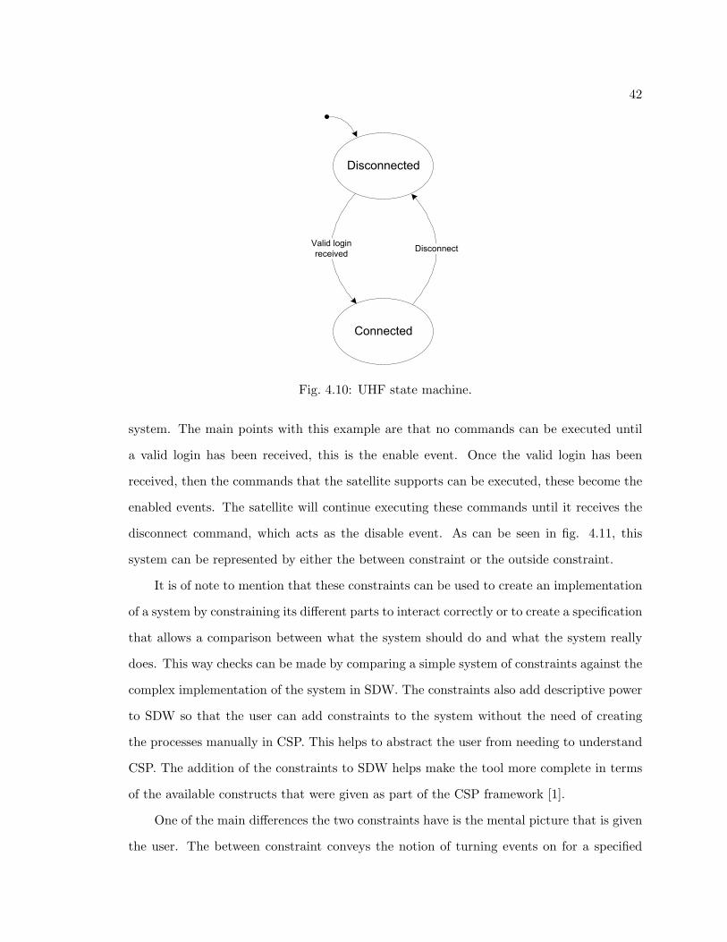
42
Valid login
receivedDisconnect
Fig. 4.10: UHF state machine.
system. The main points with this example are that no commands can be executed until
a valid login has been received, this is the enable event. Once the valid login has been
received, then the commands that the satellite supports can be executed, these become the
enabled events. The satellite will continue executing these commands until it receives the
disconnect command, which acts as the disable event. As can be seen in fig. 4.11, this
system can be represented by either the between constraint or the outside constraint.
It is of note to mention that these constraints can be used to create an implementation
of a system by constraining its different parts to interact correctly or to create a specification
that allows a comparison between what the system should do and what the system really
does. This way checks can be made by comparing a simple system of constraints against the
complex implementation of the system in SDW. The constraints also add descriptive power
to SDW so that the user can add constraints to the system without the need of creating
the processes manually in CSP. This helps to abstract the user from needing to understand
CSP. The addition of the constraints to SDW helps make the tool more complete in terms
of the available constructs that were given as part of the CSP framework [1].
One of the main differences the two constraints have is the mental picture that is given
the user. The between constraint conveys the notion of turning events on for a specified

43
Cmds enabled
Enable event:
Valid Login
Disable event:
Disconnect cmd
Cmds enabled
Enable event:
Valid Login
Disable event:
Disconnect cmd
Cmds enabled
Fig. 4.11: Constrained uplink example.
time. The outside constraint conveys the notion of turning events off for a specified time.
The outside constraint gives the notion of events starting out enabled while the between
constraint gives the notion of events starting out disabled. In the end, either constraint
could be used to represent a particular constraint, but the two notations each have cases
that they represent more concisely.
4.4 The SDW Meta-Model
This section describes SDW’s meta-model as background for the revisions and additions
made to it for this research. SDW was originally developed by Dr. Brandon Eames and
Allan McInnes. The SDW meta-model contains the rules that define how spacecraft can be
modeled. It specifies how the designer can create each spacecraft subsystem and subsystem
interactions. The meta-model is organized into different divisions to make it readable when
it becomes large and complex. Each division, known as a paradigm sheet or simply a sheet,
contains a cohesive group of components that are related to each other.
The class diagram shown in fig. 4.12 shows the meta-model’s system level components.
Each component is detailed in its own paradigm sheet. An SDW model is composed of:
• symbol specifications,
• state object specifications,

44
• external channels,
• dataflow function specifications,
• FFBD specifications.
The entire system resides in the System Folder. The system contains all applicable
specifications and also all external channels. Each paradigm is discussed in detail below.
4.4.1 Symbol Specifications
The symbol specifications sheet defines symbol sets, symbols, and tuples. Symbol sets
are how data types are defined in SDW. Symbols represent data passed from one part of a
model in SDW to another. Figure 4.13 shows the meta-model of the symbol specifications.
SymbolsSpecifications contains the SymbolSets. A symbol set is either made up of single
symbols or tuples. A tuple is made up of two or more symbols. The symbols that make up
a tuple can be from the same symbol set or different symbol sets. Tuples representing all
possible combinations of the symbols included in a tuple make up the tuple symbol set.
4.4.2 State Object Specifications
The state object specifications sheet defines the state object. A state object stores
values and can be used in an SDW model as an input to or output from a DFD function. It
is also used in an FFBD in the choice function to control an iteration or choice construct.
Figure 4.14 shows the meta-model for state objects. The state object contains only two
types of objects, a symbol set and a port. The symbol set defines what symbols can be
stored as the value in the state object; this is similar to a type declaration for a variable
in C. The state object contains both an input port and an output port. These ports allow
connections to be made in the DFD to show the flow of data to and from the state object.
4.4.3 External Channels
The external channel sheet defines the external channels that interface the model to
the rest of the world. Figure 4.15 shows the meta-model that defines the external channel.

45
System<<Model>>
FFBDSpecifications<<Model>>
SystemFolder<<Folder>>
DataflowFunctionSpecifications<<Model>>
ExternalChannel<<Model>>
StateObjectSpecifications<<Model>>
SymbolSpecifications<<Model>>
Fig. 4.12: SDW meta-model.
SymbolSet<<Model>>
Symbol<<FCO>>
TupleIndex : field
SimpleSymbol<<Atom>>
SymbolSpecifications<<Model>>
SymbolTuple<<Model>>
Fig. 4.13: SDW symbol specifications.

46
Port<<Atom>>
StateObject<<Model>>
SymbolSet<<Model>>
StateObjectSpecifications<<Model>>
Fig. 4.14: SDW state object specifications.
The port is the interface for the model to send data to or receive data from the rest of
the world. External channels are directional and only contain one port. Just like the state
object, the symbol set defines the type of data a channel accepts.
4.4.4 Dataflow Function Specifications
The dataflow function specifications sheet defines the dataflow diagram portion of
SDW. Figure 4.16 shows the meta-model for dataflow functions. Dataflow function speci-
fications contains all of the dataflow functions in the model. A dataflow function contains
both an input and an output port. Each port is associated with a symbol set that defines
the symbols that can be passed through it. Input symbols are mapped to output symbols by
the SymbolMappingConn. Dataflow functions output to either a state object or an external
ExternalChannel<<Model>>
Port<<Atom>>
SymbolSet<<Model>>
Fig. 4.15: SDW external channels.
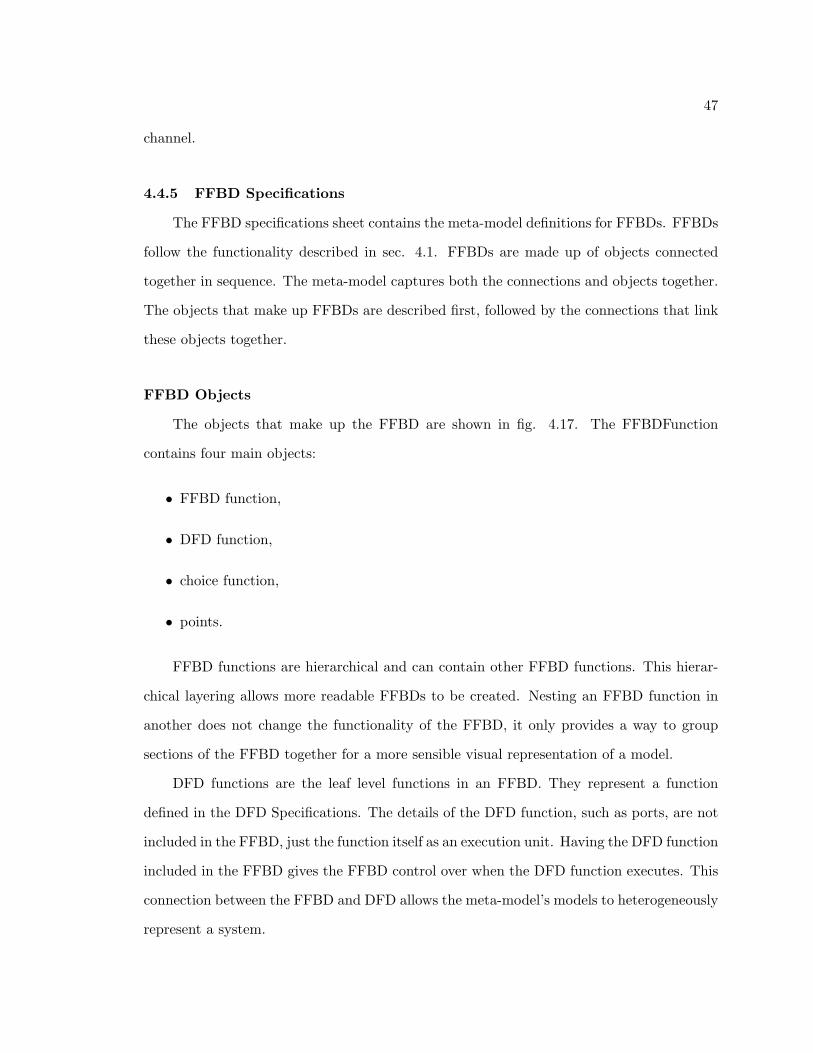
47
channel.
4.4.5 FFBD Specifications
The FFBD specifications sheet contains the meta-model definitions for FFBDs. FFBDs
follow the functionality described in sec. 4.1. FFBDs are made up of objects connected
together in sequence. The meta-model captures both the connections and objects together.
The objects that make up FFBDs are described first, followed by the connections that link
these objects together.
FFBD Objects
The objects that make up the FFBD are shown in fig. 4.17. The FFBDFunction
contains four main objects:
• FFBD function,
• DFD function,
• choice function,
• points.
FFBD functions are hierarchical and can contain other FFBD functions. This hierar-
chical layering allows more readable FFBDs to be created. Nesting an FFBD function in
another does not change the functionality of the FFBD, it only provides a way to group
sections of the FFBD together for a more sensible visual representation of a model.
DFD functions are the leaf level functions in an FFBD. They represent a function
defined in the DFD Specifications. The details of the DFD function, such as ports, are not
included in the FFBD, just the function itself as an execution unit. Having the DFD function
included in the FFBD gives the FFBD control over when the DFD function executes. This
connection between the FFBD and DFD allows the meta-model’s models to heterogeneously
represent a system.

48
SymbolMappingConn<<Connection>>
PortSymbSetConn<<Connection>>
DataflowFunction<<Model>>
Port<<Atom>>
PortToPortConn<<Connection>>
InPort<<Atom>>
OutPort<<Atom>>
DataflowFunctionSpecifications<<Model>>
StateObject<<Model>>
Symbol<<FCO>>
ExtChannel<<Model>>
SymbolSet<<Model>>
dst
src
src
dst
Fig. 4.16: SDW DFD specifications.

49
The ChoiceFunction contains the objects it needs to evaluate a stored value to deter-
mine if the condition is true or false. The StateObject contains the stored value that is the
condition of the ChoiceFunction. The SymbolSet contains all of the possible values that can
be stored in the StateObject. The GoSet is a sub-set of the symbols in SymbolSet. This
sub-set is identified by connections from GoSet to the symbols in SymbolSet that make up
the set of values that evaluate to go, or true. The connections for the GoSet to identify the
selected symbols is the GoSymbolConn.
The point represents any place in an FFBD that multiple connections must meet to-
gether. There are four types of points:
• AndPoint,
• OrPoint,
• InterfacePoint,
• ChoicePoint.
The AndPoint denotes the beginning and ending of an FFBD concurrency construct.
The OrPoint denotes the beginning and ending of an FFBD selection construct. The In-
terfacePoint denotes the entrance and exit points of an FFBD function. The ChoicePoint
denotes the beginning of an FFBD iteration or the end of an FFBD choice.
FFBD Connections
The connections that allow FFBD objects to be connected in sequence are shown in
fig. 4.18. All FFBD connections are directional to show precedence between objects. There
are five connection types:
• ChoiceGoConn,
• ChoiceNoGoConn,
• SeqObjToChoiceConn,

50
InterfacePoint<<Atom>>
AndPoint<<Atom>>
GoSet<<Atom>>
StateObject<<Model>>
GoSymbolConn<<Connection>>
Symbol<<FCO>>
ChoicePoint<<Atom>>
FFBDFunction<<Model>>
OrPoint<<Atom>>
Point<<Atom>>
ChoiceFunction<<Model>>
SymbolSet<<Model>>
FFBDSpecifications<<Model>>
SequencableObject<<FCO>>
DataflowFunction<<Model>>
Fig. 4.17: SDW FFBD meta-model objects.
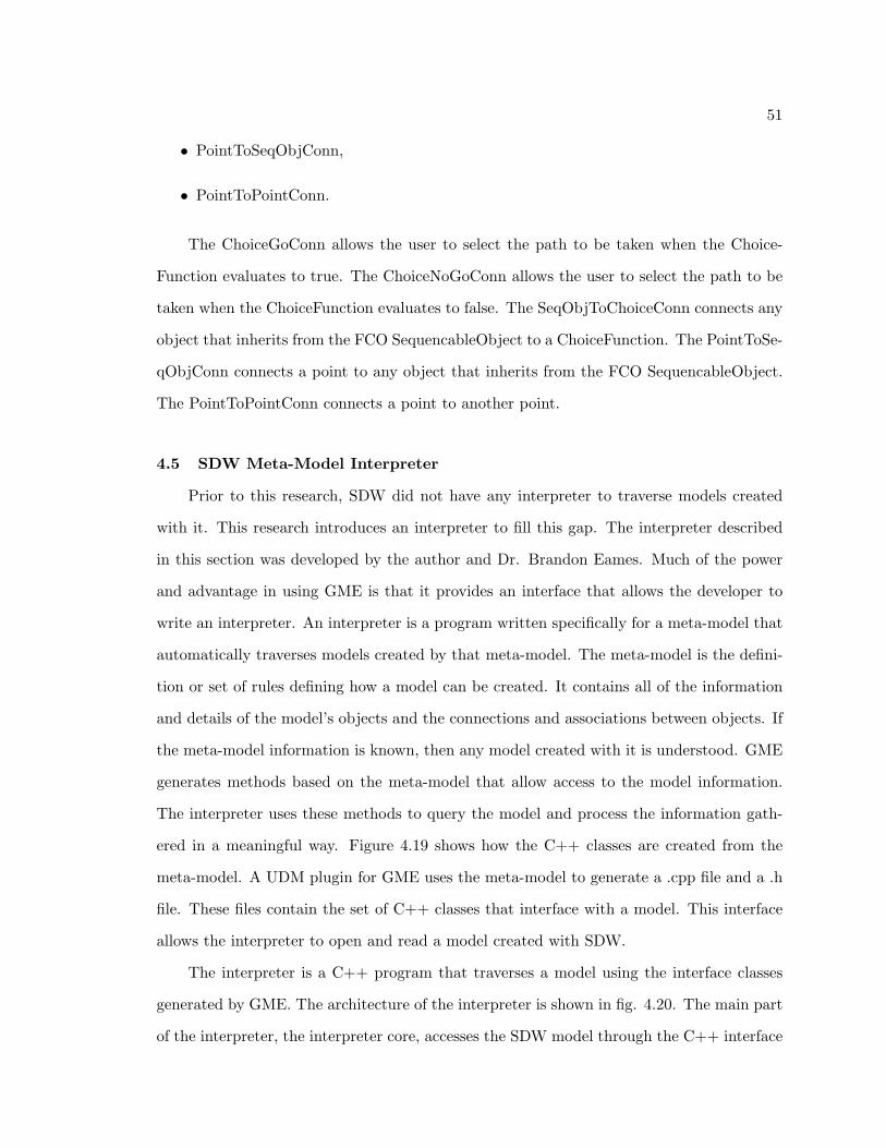
51
• PointToSeqObjConn,
• PointToPointConn.
The ChoiceGoConn allows the user to select the path to be taken when the Choice-
Function evaluates to true. The ChoiceNoGoConn allows the user to select the path to be
taken when the ChoiceFunction evaluates to false. The SeqObjToChoiceConn connects any
object that inherits from the FCO SequencableObject to a ChoiceFunction. The PointToSe-
qObjConn connects a point to any object that inherits from the FCO SequencableObject.
The PointToPointConn connects a point to another point.
4.5 SDW Meta-Model Interpreter
Prior to this research, SDW did not have any interpreter to traverse models created
with it. This research introduces an interpreter to fill this gap. The interpreter described
in this section was developed by the author and Dr. Brandon Eames. Much of the power
and advantage in using GME is that it provides an interface that allows the developer to
write an interpreter. An interpreter is a program written specifically for a meta-model that
automatically traverses models created by that meta-model. The meta-model is the defini-
tion or set of rules defining how a model can be created. It contains all of the information
and details of the model’s objects and the connections and associations between objects. If
the meta-model information is known, then any model created with it is understood. GME
generates methods based on the meta-model that allow access to the model information.
The interpreter uses these methods to query the model and process the information gath-
ered in a meaningful way. Figure 4.19 shows how the C++ classes are created from the
meta-model. A UDM plugin for GME uses the meta-model to generate a .cpp file and a .h
file. These files contain the set of C++ classes that interface with a model. This interface
allows the interpreter to open and read a model created with SDW.
The interpreter is a C++ program that traverses a model using the interface classes
generated by GME. The architecture of the interpreter is shown in fig. 4.20. The main part
of the interpreter, the interpreter core, accesses the SDW model through the C++ interface

52
ChoiceNoGoConn<<Connection>>
PointToSeqObjConn<<Connection>>
Point<<Atom>>
SeqObjToChoiceConn<<Connection>>
FFBDFunction<<Model>>
ChoiceFunction<<Model>>
SequencableObject<<FCO>>
ChoiceGoConn<<Connection>>
PointToPointConn<<Connection>>
DataflowFunction<<Model>>
src
src
src
dstdst
dst
src
dst
Fig. 4.18: SDW FFBD meta-model connections.
SDW Meta-model
UDM API Generator
C++ Interface Classes.cpp and .h files
Fig. 4.19: Meta-model C++ interface creation.
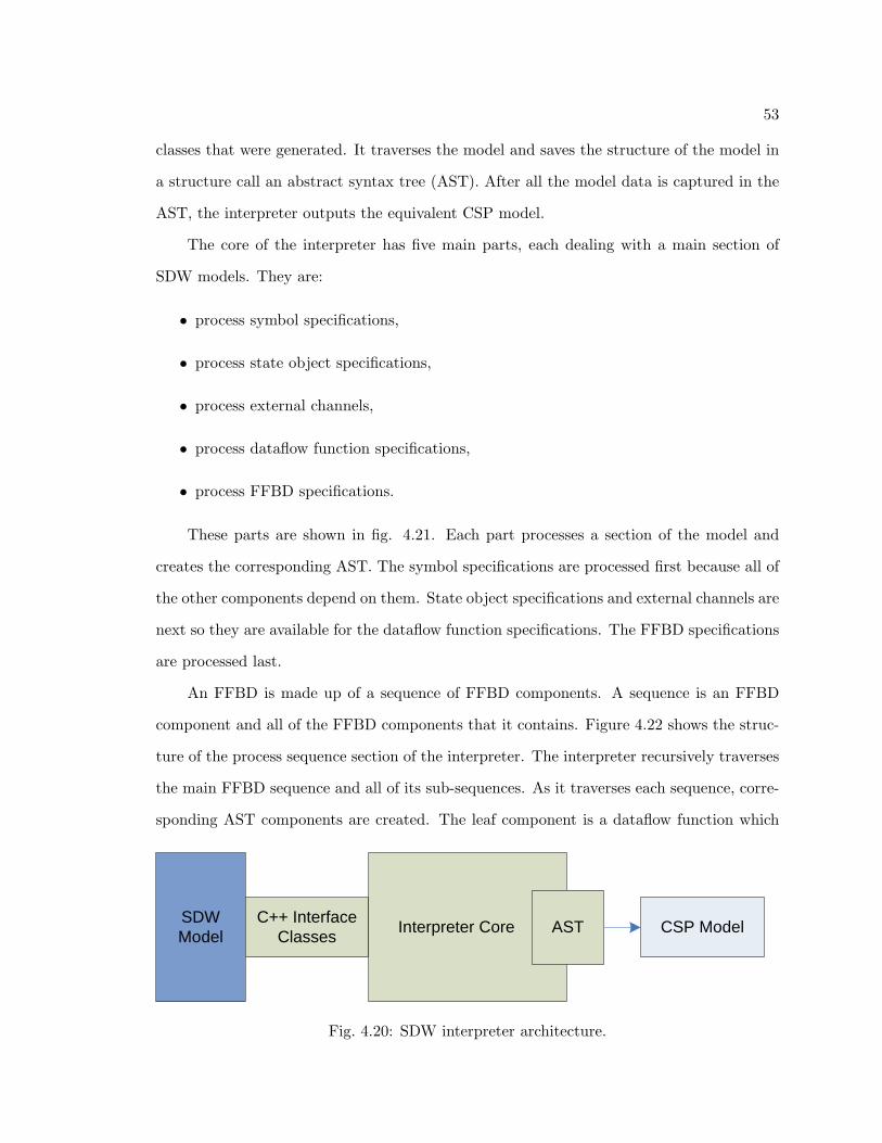
53
classes that were generated. It traverses the model and saves the structure of the model in
a structure call an abstract syntax tree (AST). After all the model data is captured in the
AST, the interpreter outputs the equivalent CSP model.
The core of the interpreter has five main parts, each dealing with a main section of
SDW models. They are:
• process symbol specifications,
• process state object specifications,
• process external channels,
• process dataflow function specifications,
• process FFBD specifications.
These parts are shown in fig. 4.21. Each part processes a section of the model and
creates the corresponding AST. The symbol specifications are processed first because all of
the other components depend on them. State object specifications and external channels are
next so they are available for the dataflow function specifications. The FFBD specifications
are processed last.
An FFBD is made up of a sequence of FFBD components. A sequence is an FFBD
component and all of the FFBD components that it contains. Figure 4.22 shows the struc-
ture of the process sequence section of the interpreter. The interpreter recursively traverses
the main FFBD sequence and all of its sub-sequences. As it traverses each sequence, corre-
sponding AST components are created. The leaf component is a dataflow function which
SDW Model
C++ Interface Classes Interpreter Core ‘ AST CSP Model
Fig. 4.20: SDW interpreter architecture.

54
cannot contain any other components. The recursion continues until the end of each se-
quence is found. The end of the main sequence indicates the interpreter has traversed the
entire FFBD specification.
4.6 SDW Meta-Model Revision
The interpreter must be able to correctly traverse any legal model created. The struc-
tures allowed in the meta-model determine the difficulty of model processing. Some struc-
tures are easily read by a human, but are difficult for a program to distinguish and un-
derstand because of ambiguities in how each part of the model fits into the overall model.
Removing these ambiguities by revising the meta-model makes the model possible to pro-
cess. The process of writing the SDW interpreter revealed ambiguities in the meta-model.
Revisions to the meta-model have removed these ambiguities. The motivation for these
revisions and the revisions themselves are described in this section. The resulting meta-
model’s models are more suited to automated interpreting. The revised meta-model also
provides a more intuitive modeling environment for the user. The following sub-sections
detail the revisions made to the meta-model as part of this research.
4.6.1 FFBD Connections Change
FFBDs connections must be intuitive for the user to use when connecting FFBD blocks
together. Modifications made to the meta-model allow all objects to connect together
unambiguously. The modified meta-model also contains fewer types of connections, resulting
in a simpler meta-model.
All four basic types of FFBD objects need to be able to connect together in any order.
Because a connection is directional, it must be described in terms of what objects it can
connect to and also connect from. This directionality is show in the meta-model by the
designations src for the source object and dst for the destination object.
The original meta-model connections in fig. 4.17 show that a point can be a source
or a destination object for the PointToPointConn connection. A point can also connect
to or from a SequencableObject by the PointToSeqObjConn connection. The lack of the

55
Interpreter Core
Process Symbol Specifications
Process State Object
Specifications
Process External Channels
Process Dataflow Function
Specifications
Process FFBD Specifications
Symbol AST
State Object AST
External Channel AST
Dataflow Function AST
FFBD AST
Process FFBD Function
Process Sequence
Fig. 4.21: SDW interpreter core structure.

56
Process Sequence
Process FFBD Function
And AST
Dataflow function
FFBD Function
Or AST
Choice AST
Iteration AST
Process Sequence
Process Sequence
Process Sequence
Dataflow AST
Process Sequence
Process Sequence
Fig. 4.22: Recursive interpreter process sequence.

57
src or dst designation on an object allows it to behave as either a source or destination
object. Since both connections can connect a point to another point, when this connec-
tion is made the user must select one of the two connections. There is no clear reason
why the user should select one connection over the other. This ambiguity was removed
by deleting the PointToPointConn connection. Because the point inherits from Sequenca-
bleObject, the PointToSeqObjConn allows a point to connect to another point, making the
PointToPointConn unnecessary.
Choice functions have ambiguities similar to the point to point connection. Choice
functions are the source for four different connections. The first two connections are the
ChoiceGoConn and ChoiceNoGoConn that show the path to take if the choice was evaluated
to true or false. The third and fourth connections, inherited from SequencableObject, are
PointToSeqObjConn and SeqObjToChoiceConn.
The PointToSeqObjConn allows a choice function to connect to any type of point.
The SeqObjToChoiceConn allows a choice function to connect to another choice function.
Both of these connections are in addition to the ChoiceGoConn and ChoiceNoGoConn. A
choice function always needs connect to other object in terms of the ChoiceGoConn and
ChoiceNoGoConn so that the path to take as a result of evaluating its condition is known.
Any other connections create confusion for the modeler when connecting the choice function
to points or other choice functions.
FFBDFunctions and DFDFunctions inherit connections from SequencableObject. Se-
quencableObject can only connect to a point or ChoiceFunction. This makes it so FFBD-
Functions and DFDFunctions cannot connect to other FFBDFunctions or DFDFunctions.
This creates a gap in the capability of the FFBD to show the order object should execute
in.
The ChoiceFunction needs to be the source of only two types of connections, the Choice-
GoConn and ChoiceNoGoConn. These two connections describe how the ChoiceFunction
can connect to any other object in the FFBD. There ChoiceFunction cannot have any other
type of connection because it must show the path to take if its condition is true or if it is

58
false. The point, FFBDFunction, and DFDFunction all need to be able to connect to each
other and the ChoiceFunction. They only need one type of connection to show precedence.
All four objects share the need to be able to connect to any other type of object in the
FFBD. Figure 4.23 shows the revised meta-model. The FCO SequencableObject is now the
destination object, with all types of connections connecting to it. All of the FFBD objects
inherit from SequencableObject which allows any of them to be the destination object of
any of the connections.
The FCO ConnSequencableObject captures the common need of the FFBDFunction,
point, and DFDFunction to connect to any other object. It separates this connection from
the ChoiceFunction since only the three objects inherit from it. This new meta-model
removes both the PointToSeqObjConn and PointToPointConn connections and replaces
them with the single connection SeqObjConn.
The revised meta-model in fig. 4.23 ensures that all objects can be connected together
unambiguously. The user is only asked to specify the type of connection when connecting
from a ChoiceFunction. Since both FFBDFunction and DFDFunction objects inherit from
a common FCO, they can be connected together to show proper precedence. Point objects
can connect to other points and also ChoiceFunctions.
4.6.2 Choice Point Change
The ChoiceFunction block is used to indicate the condition in both the FFBD choice
and the FFBD iteration constructs. In the original meta-model, they also share the same
point, ChoicePoint shown in fig. 4.17, to indicate the start of an iteration or the end of a
choice. This caused ambiguities to arise in the interpreter. When multiple iterations and/or
choice functions were nested together, it became impossible for the interpreter to tell which
point should be paired with which function. This is due to the limited knowledge that the
interpreter has about the model at the choice point or the choice model. The interpreter
is aware of the current object and the previous and next objects it is connected to. This
means if an iteration was nested inside of a choice, when the interpreter encountered the
connection point for the iteration, it could not tell if it closed the choice or marked the

59
SeqObjectConn<<Connection>>
FFBDFunction<<Model>>
ChoiceGoConn<<Connection>>
Point<<Atom>>
SequencableObject<<FCO>>
ConnSequencableObject<<FCO>>
ChoiceFunction<<Model>>
ChoiceNoGoConn<<Connection>>
DataflowFunction<<Model>>
src
src src
dst
dst dst
Fig. 4.23: FFBD connections.

60
beginning of the iteration. A look ahead method would need to be employed to extend the
interpreter’s knowledge. The look-a-head method introduced two issues.
First, the look-a-head method would greatly extend the complexity of the interpreter,
this would affect how quickly and effectively changes to the meta-model could be reflected
in the interpreter. Second, the interpreter would not know if a model it is interpreting is
constructed correctly until it had traversed to the end of the model. For small models this
is not an issue since run time would be minimal. However, as the complexity and size of the
model increases, the traversal of the model becomes increasingly complex and the runtime
could extend dramatically.
To be able to traverse models effectively without the look ahead, the interpreter needed
another way to distinguish choice and iteration points. To do this, an additional point
object was added. The additional point is called the IterationPoint, shown in fig. 4.24.
This simplifies the interpreter since when the IterationPoint is encountered, the interpreter
knows it marks the start of an FFBD iteration and can treat it as such. Likewise when
a ChoicePoint is encountered, the interpreter knows that it marks the end of an FFBD
choice. This change does not impact the connection changes described earlier because the
InterfacePoint inherits all of the characteristics of the point object.
InterfacePoint<<Atom>>
IterationPoint<<Atom>>
ChoicePoint<<Atom>>
OrPoint<<Atom>>
AndPoint<<Atom>>
Point<<Atom>>
Fig. 4.24: The point objects.

61
4.6.3 Constraints Addition
The addition of constraints to the meta-model provides more versatility to the modeler
using SDW. The original SDW does not include any constraints. The constraint addition
makes up its own sheet in the top level of the meta-model. The new SDW context diagram
is shown in fig. 4.25 with the new component ConstraintSpecifications.
The ConstraintSpecifications contains all of a model’s constraints. Figure 4.26 shows
the meta-model objects that make up the constraints. The constraint specifications contains
both between and outside constraints. The constraint model is an abstract object that
allows both the between and outside constraints to be defined as different objects with the
same components. The difference between the two constraints is how they are understood
semantically even though they share all objects in the meta-model.
Each constraint has three sets of events. These events inherit from the common ob-
ject ConstraintEvents, shown in fig. 4.26. The first set of events is represented by the
EnableEvents atom. This object indicates the events that will enable the events that are
controlled by the constraint. The second set of events is represented by the EnabledEvents
atom. This set of events are those controlled by the constraint. The third set of events is
the DisableEvents. This set represents the set of events that will disable the constrained
events.
Events in SDW are when a state object or external channel is accessed by reading or
sending a symbol. These two objects are the sources of events, as shown in fig. 4.26. The
EmptySet is included for completeness of the model. The empty set allows a set of events
to be completely disabled. Each event source may have multiple symbols pass through it.
The SymbolSet object allows the constraint events to be specified as a subset of possible
symbols over an event source.
Event sets are shown by a connection from the event source to the event set it belongs
to. The connection, EventSrcToSetConn is shown in fig. 4.27. The SymbolSet shows all
of the symbols that form events as the symbols are passed to and from the source. The
connection IncludeConn allows specific symbols to be included in the event set. The entire

62
ConstraintSpecifications<<Model>>
DataflowFunctionSpecifications<<Model>>
StateObjectSpecifications<<Model>>
FFBDSpecifications<<Model>> System
<<Model>>
ExternalChannel<<Model>>
SystemFolder<<Folder>>
SymbolSpecifications<<Model>>
Fig. 4.25: SDW context diagram.
constraint meta-model is shown in fig. 4.28.
4.7 Example SDW Model
This section gives an example of a model created in SDW and shows the corresponding
output produced by the interpreter. The SDW interpreter is able to traverse an entire
model and read all of its respective parts. The interpreter extracts all of the information
from the graphical model and creates an analyzable text model in CSP. For each part of the
model, there is a corresponding representation in CSP as described in A Formal Approach
to Specifying and Verifying Spacecraft Behavior [1].
The example model is a mux that accepts an input and produces a corresponding
output. The mux must receive a specific symbol as input first. After the mux receives this
input, it will continue to accept any input value until it receives the terminator symbol.
The mux system contains the following components:
• symbol set: A Symbols,

63
StateObject<<Model>>
ConstraintEvents<<FCO>>
EnableEvents<<Atom>>
EnabledEvents<<Atom>>
EventSource<<FCO>>
DisableEvents<<Atom>>
ConstraintSpecifications<<Model>>
SymbolSet<<Model>>
ExistingEvents<<FCO>>
Between<<Model>>
EmptySet<<Atom>>
Constraint<<Model>>
ExternalChannel<<Model>>
Outside<<Model>>
Fig. 4.26: SDW constraint objects.

64
Symbol<<FCO>>
ConstraintEvents<<FCO>>
IncludeConn<<Connection>>
Constraint<<Model>>
EventSrcToSetConn<<Connection>>
StObjSet : boolStObjSense : boolStObjTrans : bool
EventSource<<FCO>>
ExistingEvents<<FCO>>
EmptySet<<Atom>>
Fig. 4.27: SDW constraint connections.
• symbol set: B Symbols,
• state object: Current B,
• external channel: Incoming A,
• constraint: Between,
• DFD function: A to B Mux,
• FFBD.
Each component is discussed in detail below.
4.7.1 Mux Symbol Sets
A symbol is an abstraction of an object in a system. A symbol could be data, a signal
or something else, it depends on what makes sense for the system. In modeling a satellite, a
symbol might be a command or data of some kind. Symbols are grouped together in symbol
sets. Symbol sets are all declared in the symbol set specifications object. A symbol is only
defined once and in one symbol set. The symbol sets for the mux model are shown in fig.

65
EnabledEvents<<Atom>>
ConstraintEvents<<FCO>>
DisableEvents<<Atom>>
EnableEvents<<Atom>>
EventSource<<FCO>>
IncludeConn<<Connection>>
Constraint<<Model>>
ConstraintSpecifications<<Model>>
EventSrcToSetConn<<Connection>>
StObjSet : boolStObjSense : boolStObjTrans : bool
EmptySet<<Atom>>
ExistingEvents<<FCO>>
Between<<Model>>
Outside<<Model>>
SymbolSet<<Model>>
Symbol<<FCO>>
StateObject<<Model>>
ExternalChannel<<Model>>
Fig. 4.28: SDW constraint meta-model.

66
4.29. The mux model has two symbol sets, A Symbols and B Symbols. Both symbol sets
contain four symbols. The interpreter produces the following CSP for these symbol sets.
datatype A_Symbols = A1 | A2 | A3 | A4
datatype B_Symbols = B1 | B2 | B3 | B4
These two statements declare two different data types and their four associated values,
as shown in fig. 4.29.
4.7.2 Mux State Object
A state object is an object that can remember a symbol. Each state object has an
input and an output port that are both associated with a single common symbol set. Each
state object also has an initial value that is one of the symbols in its symbol set. The state
object holds the initial value at the beginning. This value is changed when a new symbol
is received on the input port. The output port allows the state object to be queried for its
current value. State objects are all defined together in the state object specifications block.
Figure 4.30 shows the state object specifications for the mux model. The mux model has
one state object, Current B. Figure 4.31 shows the inside details of the state object. It has
a symbol set that determines what values it is able to store. It also shows the initial symbol,
B1. The interpreter produces the following CSP for the state object.
channel set_Current_B : B_Symbols
channel sense_Current_B : B_Symbols
channel trans_Current_B : B_Symbols
channel sense_Current_B_FFBD : B_Symbols
A1A2A3A4
A_Symbols
B1B2B3B4
B_Symbols
Fig. 4.29: Mux symbol set specifications.

67
Current_B = AssignableState(set_Current_B,
sense_Current_B,
trans_Current_B, B1)
The four channel declarations define the channels that the state object needs. Each
channel has the data type B Symbols, which corresponds to the symbol set contained in the
state object. The last statement defines the process Current B, which is the state object
itself. The process definition uses the state objects associated channels and also the initial
value, B1, which is the last parameter in the definition.
4.7.3 Mux External Channel
An external channel is an interface to the outside world. The outside world is everything
out of the scope of the model. External channels provide a way to draw the bounds of
the model while providing a way to interact with the surrounding environment. External
channels can either be an input or an output channel. This is represented by either an
input or output port. The port is associated with a symbol set that specifies what the
external channel can receive or send. Figure 4.32 shows the external channel, Incoming A,
in the mux model. The details inside Incoming A are shown in fig. 4.33. The symbol
set A Symbols defines the data that can pass through the channel. The outport object
shows that data is coming out of the channel into the model from outside. The interpreter
produces the following channel declaration for the external channel Incoming A.
channel Incoming_A : A_Symbols
InP Out
Current_B
Fig. 4.30: Mux state object specifications.

68
InPort
InitialValue
OutPort
B1B2B3B4
B_Symbols
Fig. 4.31: Mux Current B state object.
This declaration defines the incoming channel, Incoming A, to accept symbols from the
A Symbols symbol set.
4.7.4 Mux Constraint
Constraints allow additional control of the entire system. The mux constraint Sys-
tem Enable requires the first incoming message on the channel Incoming A to be A1. It
then allows all messages over the channel until the state object Current B is set to B1. Fig-
ure 4.34 shows the between constraint System Enable. The definitions of System Enable
are shown in fig. 4.35. This shows the three event sets that make up the between con-
straint. The first set is the enable set. Figure 4.35 shows the enable object connected to
the Incoming A channel, which is in turn connected to the symbol A1. This means that
when the symbol A1 is received on Incoming A channel, the events in the enabled set are
allowed to happen. The enabled object is connected to the Incoming A channel, but there
are no symbols explicitly shown. This means that any symbol Incoming A can receive is StateObjectSpecifications
Out
Incoming_A
DataflowFunctionSpecificationsFFBDSpecifications
SymbolSpecifications
Fig. 4.32: Mux external channel Incoming A.

69
A1A2A3A4
A_Symbols
OutPort
Fig. 4.33: Mux external channel Incoming A internal definition.
allowed to be passed over the channel. The disable object is connected to the state object
Current B, which is connected to the symbol B1. This means when Current B is set to
B1, then the events in the enabled set are no longer allowed. The interpreter produces the
following processes for the constraint.
alph_System_Enable = {|Incoming_A.A1, set_Current_B.B1, Incoming_A|}
System_Enable = Between({|Incoming_A.A1|},
{|set_Current_B.B1|},
{|Incoming_A|})
ConstraintSet = {(alph_System_Enable, System_Enable)}
aCNet = aConstraintNet(ConstraintSet)
CNet = ConstraintNet(ConstraintSet)
The first statement creates an alphabet, or set, of all events, alph System Enable,
used by the constraint. The second statement is the constraint process, System Enable,
with its enable, enabled, and disable event sets. The third statement combines all of the
constraints and their alphabets (although in this example there is only one) as a set of pairs.
The ConstraintSet is used to create the constraint net process, CNet, and its alphabet,
aCNet. Both of these are used to integrate all constraints in the complete system process.

70
System_Enable
Fig. 4.34: Mux constraint specifications.
Out
Incoming_A
InP Out
Current_B
A1A2A3A4
A_Symbols
B1B2B3B4
B_Symbols
Out
Incoming_A
Fig. 4.35: Mux between constraint.
4.7.5 Mux DFD
In SDW, a DFD function has an input port and an output port. Every DFD function
must have an input source and an output destination. It is possible for the function to have
multiple ports. Each port must be associated with a symbol set that defines the symbols
that are allowed to go through it. Figure 4.36 shows the mux DFD function. It receives
its input from the incoming channel Incoming A, and sends its output to the state object
Current B. The function mapping of A to B Mux is shown in fig. 4.37. The input port
can receive symbols in the symbol set A Symbols. The input symbols are mapped to the
symbol set B Symbols and passed to the output port. Each input symbol must map to one
of the output symbols. The interpreter produces the following output for the DFD function
A to B Mux.
-- Function <A_to_B_Mux>
f_A_to_B_Mux = {(A1, B2),
(A2, B3),
(A3, B4),
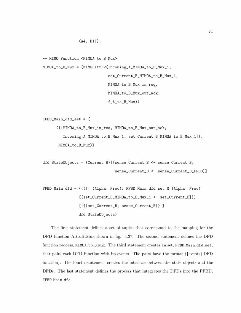
71
(A4, B1)}
-- MIMO Function <MIMOA_to_B_Mux>
MIMOA_to_B_Mux = (MIMOLiftF2(Incoming_A_MIMOA_to_B_Mux_1,
set_Current_B_MIMOA_to_B_Mux_1,
MIMOA_to_B_Mux_in_req,
MIMOA_to_B_Mux_out_ack,
f_A_to_B_Mux))
FFBD_Main_dfd_set = {
({|MIMOA_to_B_Mux_in_req, MIMOA_to_B_Mux_out_ack,
Incoming_A_MIMOA_to_B_Mux_1, set_Current_B_MIMOA_to_B_Mux_1|},
MIMOA_to_B_Mux)}
dfd_StateObjects = (Current_B)[[sense_Current_B <- sense_Current_B,
sense_Current_B <- sense_Current_B_FFBD]]
FFBD_Main_dfd = (((|| (Alpha, Proc): FFBD_Main_dfd_set @ [Alpha] Proc)
[[set_Current_B_MIMOA_to_B_Mux_1 <- set_Current_B]])
[|{|set_Current_B, sense_Current_B|}|]
dfd_StateObjects)
The first statement defines a set of tuples that correspond to the mapping for the
DFD function A to B Mux shown in fig. 4.37. The second statement defines the DFD
function process, MIMOA to B Mux. The third statement creates an set, FFBD Main dfd set,
that pairs each DFD function with its events. The pairs have the format ({events},DFD
function). The fourth statement creates the interface between the state objects and the
DFDs. The last statement defines the process that integrates the DFDs into the FFBD,
FFBD Main dfd.
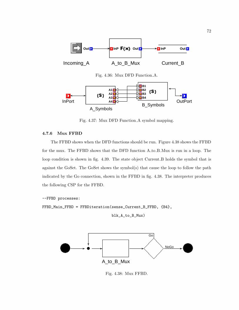
72
InP Out
A_to_B_Mux
Out
Incoming_A
InP Out
Current_B
Fig. 4.36: Mux DFD Function A.
B1B2B3B4
B_Symbols
A1A2A3A4
A_Symbols
OutPortInPort
Fig. 4.37: Mux DFD Function A symbol mapping.
4.7.6 Mux FFBD
The FFBD shows when the DFD functions should be run. Figure 4.38 shows the FFBD
for the mux. The FFBD shows that the DFD function A to B Mux is run in a loop. The
loop condition is shown in fig. 4.39. The state object Current B holds the symbol that is
against the GoSet. The GoSet shows the symbol(s) that cause the loop to follow the path
indicated by the Go connection, shown in the FFBD in fig. 4.38. The interpreter produces
the following CSP for the FFBD.
--FFBD processes:
FFBD_Main_FFBD = FFBDiteration(sense_Current_B_FFBD, {B4},
blk_A_to_B_Mux)
A_to_B_Mux
NoGo
Go
Fig. 4.38: Mux FFBD.

73
FFBD_Main = ((FFBD_Main_dfd
[|{|MIMOA_to_B_Mux_in_req, MIMOA_to_B_Mux_out_ack|}|]
FFBD_Main_FFBD)
[|aCNet|]
CNet)
[[Incoming_A_MIMOA_to_B_Mux_1<-Incoming_A]]
The first process declared, FFBD Main FFBD, represents the FFBD shown in fig. 4.38. It
includes the iteration and also the DFD function A to B Mux. The second process declared,
FFBD Main, is the complete heterogeneous system, combining the DFD, constraint, and the
FFBD into one process.
4.8 Conclusion
The SDW interpreter creates the link between SDW and the analyzable CSP constructs
of the Spacecraft Behavior Framework Library [1]. SDW uses the modeling capabilities
of GME to bring DFDs and FFBDs together in a heterogeneous modeling environment.
GME provides a flexible method for tool creation. It also provides a customizable interface
that links SDW to the CSP libraries developed in A Formal Approach to Specifying and
Verifying Spacecraft Behavior [1]. Representing a system graphically allows the user to
focus on what the system does or is supposed to do without worrying about how to create
an analyzable model. Including constraints in SDW allows more flexibility to accurately
GoSet
B1B2B3B4
B_Symbols
InP Out
Current_B
Fig. 4.39: Mux FFBD iteration condition.
74
represent a model. The interpreter is able to create the analyzable CSP version of the
graphically created system.
The author’s additions to the SDW tool include the revisions to the meta-model, the
addition of constraints in the meta-model, parts of the interpreter including the top-level
structure of the interpreter’s core, traversing FFBDs, traversing constraints, and portions
of the AST.

75
Chapter 5
Modeling TOROID II
This chapter discusses different approaches to modeling TOROID’s telemetry manager.
One approach is discussed in detail along with the resulting model. The model is analyzed
with a formal verification tool. A mathematical analysis is also described that supports the
results of the verification tool.
5.1 Approaches to Modeling the Telemetry Manager
There are several different approaches to creating a model of the telemetry manager
using SDW. The approaches include modeling the interacting tasks, modeling the flow
of data, or combining task interaction and dataflow together. This section discusses the
different approaches from the perspective of the SDW tool and the Spacecraft Behavior
Framework [1].
5.1.1 SDW Task Modeling
Task modeling represents all telemetry manager tasks and their interactions. TOROID’s
telemetry manager is made up of several buffers. These buffers are accessed by concurrently
running periodic tasks. Each buffer has an associated read and write process. Each task’s
period is controlled by a binary semaphore and a timer, as described in sec. 3.3.
A detailed model of the tasks comprising the telemetry manager requires a method of
representing task control. This requires a representation of semaphores, timers that control
when the semaphores become available, and tasks controlled by the semaphores. SDW
represents a variable, such as data or a semaphore, with a state object. State objects are
accessed by FFBD conditions or a DFD function and can be written to by a DFD function.
Accessing and writing to a state object takes several steps in the CSP that is generated.

76
When two different conditions or functions are trying to access the same state object at the
same time, there is no guarantee of mutual exclusion. When the task takes its semaphore,
it must check that the semaphore is available. If the semaphore is not available, the task
must wait until it is. When the semaphore becomes available, the task sets it to unavailable
and then continues execution.
An SDW state object cannot guarantee correct behavior as a semaphore. It has no
interface that allows mutually exclusive access to it. For this reason, tasks cannot be
represented in SDW with a semaphore control structure.
5.1.2 Dataflow Modeling
A dataflow model can represent data at several different levels of detail. At the most
detailed level the bytes that make up the data flowing in and out of the buffers is represented.
The bytes are gathered from the different source buffers and formated into the PCM page
format in the main telemetry buffer. The number of bytes flowing through each buffer plays
an important role in determining the size each buffer needs to be. However, modeling at
the byte level quickly leads to a model that is too large to verify.
Since modeling at the byte level yields an untractable verification problem, a higher
level of abstraction may result in a verifiable model. In the main loop of the telemetry
manager a minor frames are created. For each minor frame, a set amount of data is read
from each source buffer. The amount of data read is the same from one iteration to the
next. The dataflow model represents the flow of data and not the contents of the actual
data. Each buffer has data written and read to and from it in set amounts. Because the
data quantities do not vary, representing data as blocks of bytes reduces the size of the
model.
Building and Writing Single Pages Model
Setting the block size read from each buffer by the telemetry manager to the amount of
data required for one PCM page gives a simpler model. To further minimize the complexity
of the model, the source data buffers can be grouped together. From sec. 3.3 the following

77
groupings can be made. The housekeeping and TQR are combined into one source. The
image data remains by itself. The science data is combined into one science source. Using
these groupings, the telemetry manager is represented in the model by four main parts:
• build page,
• housekeeping buffer process,
• image buffer process,
• science buffer process.
These four blocks are combined together in parallel as shown in fig. 5.1. The BuildPage
function is shown in fig. 5.2. It implements the functionality of the main telemetry manager
loop given in sec. 3.3. It performs the following functions in order:
1. Read housekeeping buffer,
2. Read image buffer,
3. Read science buffer,
4. Write telemetry buffer to flash memory,
5. Reset telemetry buffer.
These functions show how the data is written to the telemetry buffer in the order
determined by the PCM matrix. BuildPage is iterated in a loop.
Each of the buffer processes writes data to the buffer. The buffer is represented by
state object that can have three different states. The states are empty, partially full, or full.
Each buffer can change state as data is written to it or read from it, according to the state
diagram given in fig. 5.3.
The state diagram is implemented for the image buffer in fig. 5.4. The DFD functions
model the write transitions shown in fig. 5.3. The first choice function checks if the buffer
state is empty. If it is, the Go path is connected to the IMG toP, which sets the buffer state

78
SCIBufProc
HKBufProc
IMGBufProc
BuildPage
Fig. 5.1: FFBD of the building single pages model.
ReadIMGReadHK WritePCMtoFlash ResetTelBufReadSCI
NoGo
Go
Fig. 5.2: FFBD of the BuildPage function.
Empty Partially full Full
write
read
write
read
write
read
Under-flow
Over-flow
read write
Fig. 5.3: Three state buffer model.

79
to partially full. Otherwise, the NoGo path is connected to a second condition that checks
if the buffer state is partially full. If it is, the Go path connects to the OR construct that
lets one of two functions, IMG toP or IMG toF, execute. IMG toP keeps the buffer state
at partially full. IMG toF sets the buffer state to full. If the second condition follows the
NoGo path, an error condition is encountered because the image buffer overflows.
Figure 5.5 shows the ReadIMG function. The DFD functions model the read transitions
in fig. 5.3. First condition checks if the buffer is full. If it is, the Go path is followed to
the IMG readToP DFD function which sets the image buffer to partially full. If the image
buffer is not full, the NoGo path leads to a second condition that checks if the buffer is
partially full. If it is, the Go path allows one of two functions to execute, IMG readToP or
IMG readToE. If the buffer is not partially full, the NoGo path leads to an error condition
because the image buffer has an underflow error. The underflow error indicates that there
was no data to be read when it was required.
An advantage of this method is that the buffer size does not need to be specified. The
buffer only has three states which represents the data at a higher level than bytes and
simplifies the state space of the model. The model diverges slightly from the system in that
it writes single pages to flash instead of accumulating eight and then writing. However, this
model still captures the interaction between the processes writing to the buffers and the
telemetry manager reading from them. The next modeling approach looks at representing
the eight pages.
Building Eight Pages Model
If the buffers are assumed to work correctly, the model can focus on representing the
system formatting eight pages of data instead of a single page. In this model data is rep-
resented as an indivisible page as opposed to a page composed of data from each source
buffer as in the single page model. Figure 5.6 shows the SDW FFBD model implementation.
The model gathers data from the buffers as a complete page of data in the function Read-
PCMpage. When eight pages have been collected, they are written flash by the function
WritePCMtoFlash. The page buffer is reset by the function ResetPageBuffer. The flash

80IMGBufProcParadigm: SpacecraftDesignWorkbench_C Project: BuildMinorFrames Model: FFBDFunction Aspect: FFBDModeling Time: Fri Sep 12 10:14:52 AM
IMG_overflow
IMG_toP
IMG_toP
IMG_toF
NoGo
Go
NoGo
Go
NoGoGo
Fig. 5.4: The image buffer write FFBD.
writeToTelBuf
IMG_readToP
IMG_readToP
IMG_readToE
IMG_underflow
NoGo
Go
Go
NoGo
Fig. 5.5: The image buffer read FFBD.

81
memory is represented by an external channel, since it is out of the scope of the model.
This method represents data at a level that is reasonable to model using SDW. Repre-
senting eight buffer states versus 64 bytes per minor frame or 256 minor frames per page is
a size that can be easily drawn by a user without additional automated tool support. It also
allows the model to ignore the lower-level details of how the data flows in the source buffers
and clearly show what is happening at the top level of the telemetry manager. While this
model may work well to represent the telemetry manager in a complete system model, it is
unable to capture much useful information about the telemetry manager itself.
Alternating Buffer Model
Another approach to modeling the flow of data in the telemetry manager is by modeling
the buffers used to format data according to the PCM matrix. The telemetry manager uses
two buffers to collect and format the science and housekeeping data. These buffers are
designated ping and pong because they are an alternating pair of buffers, one is being
written to while the other is being read. This approach treats incoming data as coming
from one source and focuses on handling the ping and pong buffers.
Figure 5.7 shows the top-level FFBD of the alternating buffer model with its two FFBD
functions running together in parallel. The alternating buffer model works to capture the
relationship between the ping pong buffers as they are read and written to. This model
represents the telemetry manager system in two parts, the telemetry manager itself that
gathers the data into the telemetry buffer and a process that writes the telemetry buffer
to flash. These two processes run together in parallel. The telemetry manager, depicted in
detail in fig. 5.8, picks a buffer, ping or pong, fills the buffer and repeats. In picking the
TelMgrParadigm: SpacecraftDesignWorkbench_C Project: Root Folder Model: FFBDFunction Aspect: FFBDModeling Time: Fri Sep 12 09:36:53 AM
ReadPCMpage WritePCMtoFlash ResetPageBuffer
Go
NoGo
Go
NoGo
Fig. 5.6: Model building eight pages.

82
buffer it alternates between ping and pong. The WriteBufferToFlash function, shown in fig.
5.9, takes the buffer that is full, ping or pong, and writes it to flash. Flash is represented
in this model as an external channel.
This model gives a simpler model of the behavior of the telemetry manager. Unfortu-
nately, it is too simple and little insight can be gained about its behavior from this model.
In the actual telemetry manager implementation, it takes a certain amount of time to fill
the ping or pong buffer. While one buffer is being filled, the other is being emptied. Time is
the determining factor as to whether or not the ping pong buffer system will work. However,
the model does not represent time and so it cannot answer the question of whether the real
system will work.
5.1.3 CSP Bounded Non-Blocking Buffer Model
CSP provides an alternate, more detailed approach to modeling a buffer. This modeling
approach explores a bounded blocking buffer process that McInnes introduces as part of
the Spacecraft Behavior Framework Library [1]. A modified version of this buffer process
represents how the buffers in the telemetry manager behave.
The CSP bounded blocking buffer inputs and outputs symbols. It can hold up to a
specified maximum number of symbols. Once this limit is reached, it no longer accepts
inputs. The buffer only outputs a value after a value is put in it, so the amount of data
in must equal the amount of data out. If data is read when the buffer is empty, it blocks
until data is written to it and then allows the data to be read. The buffers that compose
FFBDFunctionParadigm: SpacecraftDesignWorkbench_C Project: Root Folder Model: FFBDFunction Aspect: FFBDModeling Time: Fri Sep 12 10:55:41 AM
TelemetryManager
WriteBufferToFlash
Fig. 5.7: Alternating buffer model.

83
TelemetryManagerParadigm: SpacecraftDesignWorkbench_C Project: Root Folder Model: FFBDFunction Aspect: FFBDModeling Time: Fri Sep 12 10:57:47 AM
FillBufferPickBuffer
NoGo
Go
Fig. 5.8: Telemetry manager FFBD function.
WriteBufferToFlashParadigm: SpacecraftDesignWorkbench_C Project: Root Folder Model: FFBDFunction Aspect: FFBDModeling Time: Fri Sep 12 11:05:18 AM
PongToFlash ResetPong
PingToFlash ResetPingGo
NoGo
Fig. 5.9: WriteBufferToFlash FFBD.
TOROID’s telemetry system return the value zero when the buffer is empty and data is
requested. This varies slightly from the bounded blocking buffer described by McInnes in
that it only blocks inputs when the buffer is full and returns a default data value when the
buffer is read while it is empty.
The bounded blocking buffer serves as a basis to create a buffer process that matches
the telemetry manager buffers. The bounded non-blocking buffer is given by the following
CSP process.
BoundedNonblockingBuffer(in, out, N, empty) =
let
Buff(s) =
(#s < N & in?x -> Buff(s^<x>))
[]
(#s > 0 & out!head(s) -> Buff(tail(s)))
[]

84
(#s == 0 & out!empty -> Buff(<>))
within Buff(<>)
The non-blocking buffer has four input parameters.
• in
• out
• N
• empty
The first parameter, in, is the channel used to write data to the buffer. The second
parameter, out, is the channel used to read data from the buffer. The third parameter, N, is
the number of symbols that the buffer can accept and hold. The fourth parameter, empty,
is the symbol that is sent when the buffer is empty and data is requested.
Inside the bounded non-blocking buffer process is the Buff(s) process that stores all
of the input data in the same order it is received. Buff(s) follow three different paths. The
first path,
#s < N & in?x -> Buff(s^<x>),
allows symbols to be sent to the buffer and stored. This is only allowed if the number of
symbols stored in s, denoted by #s, is less than the total number of symbols accepted by
the buffer. Data is sent over the in channel, which accepts an input x and passes it to the
Buff process. The data represented by x is added to the current set of data, s. The second
path,
#s > 0 & out!head(s) -> Buff(tail(s)),
allows the next symbol in the buffer to be sent over the out channel. The next symbol is
taken from the “head” of the set s. The buffer stores data in a first in first out order. This
path is only available if there is currently data stored in the buffer. The third path,

85
#s == 0 & out!empty -> Buff(<>),
allows the empty symbol to be sent over the out channel when the buffer is read, but no
symbols are currently stored in the buffer.
The bounded non-blocking buffer represents the buffers used in the telemetry manager.
Each buffer has a default value to return in the event that data is requested when the buffer
is empty.
The problem with this modeling approach is how data is represented. The buffer is
concerned with storing data written to it and outputting data read from it in order. This
means that data is represented as having specific values. In analyzing the telemetry manager
software, the actual values that the data has do not matter. What matters is how much
data flows through the buffer and at what rates. This approach does not treat any of these
questions, but is concerned with the values of the data. It does not separate data content
from the modeling the flow of data.
5.1.4 CSP Telemetry Manager Buffer Model
This model uses multiple interacting buffers that are synchronized by time. This is
a more detailed CSP model of the telemetry manager that integrates time with a data
independent buffer representation. The addition of time allows multiple buffers to interact
with each other at a set pace. The data independent buffer represents amounts of data
and not actual data values. SDW does not provide a time construct nor a simple way to
model a buffer that can contain many different amounts of data. The Spacecraft Behavior
Framework Library does not provide a representation of time, but it does provide another
process for modeling a buffer. This process is described in detail in the next section.
To support a multi-buffer model of the telemetry manager, this thesis introduces a time
process. This process allows other processes to run at a given period. The CSP telemetry
manager model is a system of four source buffers that receive data at set periods. These
source buffers represent the housekeeping, image data, and science buffers in the telemetry

86
manager. A fifth buffer represents the telemetry manager buffer that formats data from the
source buffers. All five of these buffers are synchronized together by time.
The remainder of this chapter discusses this model in detail. The time process is given
and described along with its application to controlling a buffer. The CSP for the model is
given as well as the results of the modeling and FDR analysis. A separate mathematical
analysis is also given that supports the results of the FDR tool.
5.2 CSP Telemetry Manager Buffer Model
Data collection on the TOROID satellite is periodic. The different science data, the
system voltages and currents, the onboard temperatures and other system data are all
sampled at different periodic rates as well as in different data block sizes. All of these
various sources of data are fed into the telemetry stream and stored onboard until the
ground station is contacted, at which point the data is transmitted to the ground. The
periodic nature of these buffers requires a method of modeling the periods of the buffers’
read and write tasks as well as the buffers.
This section discusses the details for the modeling approach selected in the last section.
There are two main parts to this approach. First, representing data and the buffers that
hold it. Second, synchronizing the periodic processes that make up the buffer using a
representation of time. Both data and buffer modeling and time modeling are described
in this section. After these have been described, an example of combining the two parts
is presented. A system of a single buffer with periodic read and write processes is shown.
This system is expanded into a model of the Telemetry Manager.
5.2.1 Data and Buffer Modeling
Modeling data flowing through a buffer requires a way to represent both the data and
the buffer. A model does not necessarily need to fully represent data in a real system. The
model needs to represent the aspects of the data that impact the system’s behavior. In
the telemetry manager, the amount of data a buffer holds at a particular instance of time
affects if the buffer can accept more data or if there is enough data to fill a read request.

87
The model of a buffer needs to know how much data it holds. It is not concerned with the
type of data it holds, the data values, or what data arrived first.
A model representing data as quantities allows further simplifying data by grouping it
together as blocks. Consider a buffer with periodic tasks that write to and read from it.
The write task always writes five bytes and the read task always reads ten bytes. The data
can be represented by dividing the data amounts by the greatest common divisor. This
results in an amount written of one and an amount read of two. This simplifies the model
considerably because now instead of tracking how many individual bytes are in the buffer,
the data is described in terms of blocks.
McInnes describes another construct that is somewhat similar to the bounded blocking
buffer called the quantitative resource. The quantitative resource models a resource that
has a specific amount of the resource available. The resource is anything in the system that
has a finite quantity available. Possible resources could be power, processors, or memory.
A buffer represents an allocated amount of memory for data storage. The quantitative
resource is suited to model the behavior of a buffer at a level that abstracts the the actual
data a buffer contains to the amount of data the buffer has at a given time.
This approach of modeling data and buffers gives the foundation for a model that can
answer the question of how large a buffer or set of buffers should be. A buffer has an in
flow of data and also an out flow. Buffers are a finite size, so the amount of data in must
equal the amount of data out. In a real system the number of bytes in per second must
equal the number of bytes out per second.
5.2.2 Modeling Time
A model of the periodic telemetry manager tasks requires a way to represent time. The
buffers are written to and read from by periodic tasks. A set of source buffers are read by
the telemetry buffer, see sec. 3.3. This means that all of the buffers are linked together and
must be synchronized relative to each other. This section introduces a global time process
and task timers that create a way for periodic tasks to be synchronized with each other.

88
Global Time
For periodic tasks to interact with each other consistently each period, they must
synchronize on a common event. This common event is provided by the process,
GTIME = global_tick -> GTIME.
The global timer process GTIME sends the event global tick and then repeats itself. Pe-
riodic tasks are able to synchronize on this global tick event, enabling them to run at the
correct rates relative to one another.
Task Timer
Every periodic task requires a timer to keep track of its period by synchronizing with
the global time. Individual task timers are represented by the following process.
TIMER(ctick,p,sync) =
if ctick == 0
then sync -> sync -> TIMER(p,p,sync)
else global_tick -> TIMER(ctick-1,p,sync)
The process TIMER has three parameters:
• ctick,
• p,
• sync.
The parameter ctick is the current period counter, counting down from the number of ticks
per period. Each time there is a global tick, ctick is decremented. The parameter p is
the period of the timer. The parameter sync is the event to synchronize on when the period
counter ctick reaches zero. When the sync event occurs two times, the timer is restarted
with the period p. There must be two sync events to ensure that a task executes on the
period, not before or after. Each task needing a periodic timer has a separate instantiation
of the TIMER process. Timer processes can be combined together in CSP to create a time

89
net. A time net is a combination of all timer processes into one process to make complex
systems more readable. This time net is adapted from the constraint net given in A Formal
Approach to Specifying and Verifying Spacecraft Behavior [1] and is given by the following
processes.
TIMENET(Ttup) = (|| (pS,PT):Ttup @ [union(pS,{global_tick})] PT)
[| {global_tick} |]
GTIME
TIMESYNC(Ttup) = Union({aT | (aT,T) <- Ttup})
The parameter Ttup is a set of tuples. Each tuple is made up of a timer’s sync event and
the name of the timer process, shown by the tuple (pS,PT), respectively. The first line of
the TIMENET process places all timer tasks running concurrently together. The second and
third line places all of the timer tasks running concurrently with the global timer process
GTIME and synchronizing its event, global tick. The time net creates one single timer
process that embodies all of the individual timer processes. TIMESYNC is not a process, but
a set of events containing all of the timer processes’ sync events. This to allow the TIMENET
to be integrated into a system as a parallel process synchronizing each timer process on its
respective sync event.
Timed Tasks
The global timer only needs to capture the level of granularity that will allow other
tasks to run in multiples of it. For example, in fig. 5.10, task 1 has the smallest period, and
task 2 has a period that is twice the period of task 1. This means that the global clock has
a period equal to the period of task 1.
Task two’s period is not required to be a multiple of task one. The periods for tasks
one and two can also be expressed as a ratio of each other. The ratio is described in terms
of global clock ticks. Figure 5.11 shows tasks one and two where task two executes twice

90
Task 1 Task 1 Task 1
Task 2 Task 2
Task 1
Fig. 5.10: Two-to-one periodic task timeline.
for every three executions of task one. Task one has a period of two global clock ticks and
task two has a period of three global clock ticks.
In this case task one has to have its period described by two global ticks and task two
with a period of three global ticks. All task periods must be described in terms of an integer
number of clock ticks.
Individual tasks synchronize their periods with the global timer. Figure 5.12 illustrates
how a task is synchronized to the global clock. The task WriteBuf writes data to its
buffer and repeats. The WriteBuf Task Timer keeps track of the WriteBuf task’s period
by decrementing a counter every time that there is a global clock tick. The dotted lines
show the events that must happen at the same time. Note that they must occur together,
therefore, if the WriteBuf Task Timer process is not ready for the global clock tick event,
then the global clock process must wait until it is ready. If another timed task were to be
added to the system, it would have to run at given rate relative to WriteBuf Task to allow
both of their periods to be controlled by the rate at which the global clock runs.
In cases where there are multiple individual task timers, each of which will synchronize
with the global clock. Each task timer must have its own unique sync event. If one of the
systems that one of the task timers depends on should deadlock, the rest of the system will
Task 1 Task 1 Task 1
Task 2 Task 2
Fig. 5.11: Two-to-three periodic task timeline.

91
WriteBuf Task WriteBuf Task Timer Global Clock
Event Synchronizations
yes no
Fig. 5.12: Periodic task synchronization.

92
deadlock as well. This means that each individual task model must be deadlock free before
it can be integrated into the complete system. This is required for any system to work
correctly. All of the task timers can be grouped into one process for ease of integration
into the system model. The CSP processes that capture the global time and also allow
individual task timers are given in Appendix A.
5.2.3 Timed CSP Buffer Model
The buffer data abstraction and task timers provide a foundation to create a timed
buffer system in CSP. This buffer system is expanded to a model of the telemetry manager
later in sec. 5.2.4. The task timer allows a buffer to gather data at a given periodic rate.
A timed buffer has three components, the buffer, a periodic task that writes data to the
buffer, and a periodic task that reads from it. Figure 5.12 shows a task that writes to a
buffer which synchronizes on a global clock tick. The task that reads the buffer has the
same structure, but may have a different period. Figure 5.13 shows how the timed buffer
functions with a task writing at one period and another task reading at another period.
For a finite buffer to not overflow, the amount of data in per second must equal the
amount of data out per second. The task that writes data to the buffer must synchronize on
a timer that is set to the write period. The same goes for the read task, it must synchronize
on a timer that is set to the period of the read task. In this manner the read and write tasks
are synchronized so that they only execute on their periods. But they are also required to
execute on their periods, not earlier or later. The requirement that the data in equal the
data out is described by the relation shown in eq. (5.1), where
Bufferdata datadata data
Fig. 5.13: Timed buffer.

93
• ra is the amount of data read,
• rp is the period at which data is read,
• wa is the amount of data written,
• wp is the period at which data is written.
ra/rp = wa/wp (5.1)
The CSP model implements the buffer system in fig. 5.13. It consists of a buffer,
represented as a quantitative resource, a timed write process that writes to the buffer and
a timed process that reads from the buffer. The timed read and write processes maintain
the buffer’s balance of data in and data out as required by eq. (5.1). Inputs to the model
are the maximum buffer size and the read and write processes’ periods and amounts of data
from eq. (5.1). The machine readable CSP for a single timed buffer is given below.
-- Quantitative Resource buffer parameters
MAX = 10
MIN = 0
INIT = 0
-- Timer process parameters
WPeriod = 3
WAmount = 6
RPeriod = 2
RAmount = -4
-- Quantitative Resource channels
channel io:{ -MAX..MAX}
channel read,trans: {MIN..MAX}

94
-- Timer sync events
channel sc0timeWrite, sc0timeRead
-- Write and Read processes
QRWRITE = sc0timeWrite -> io!WAmount -> sc0timeWrite -> QRWRITE
QRREAD = sc0timeRead -> io!RAmount -> sc0timeRead -> QRREAD
-- Quantitative resource
QR = QuantResource(io,read,trans,MIN,MAX,INIT)
-- Write and Read process timers
SC0TW = TIMER(0,WPeriod,sc0timeWrite)
SC0TR = TIMER(RPeriod,RPeriod,sc0timeRead)
-- System
aTime = {({sc0timeRead},SC0TR),
({sc0timeWrite},SC0TW)}
TNET = TIMENET(aTime)
aTnet = TIMESYNC(aTime)
SYS = ((QRREAD ||| QRWRITE) [|{|io|}|] QR) [| aTnet |] TNET
-- Check that system never throws an exception indicating
-- overflow or underflow of the buffer
assert STOP [T= SYS \ diff(Events,{|qr_exception|}
The quantitative resource parameters are used to initialize the quantitative resource

95
that represents the buffer. MAX and MIN are the upper and lower bounds of the quantita-
tive resource. The timer process parameters define the read and write periods and data
amounts. The negative number represents data being read from the quantitative resource.
The quantitative resource channel declarations include all of the channels needed by the
quantitative resource. The io channel is used by the read and write processes to read and
write data to the quantitative resource. The read channel is a channel that allows the
current value held by the quantitative resource to be looked at without changing it. It is
part of the quantitative resource construct, however it is not used in this model. The timer
sync events give the channel declarations needed for the timed read and write processes.
These events are the events that enforce the read and write processes to read and write on
their respective periods.
The process definitions follow the parameters and channel declarations. The write and
read processes are QRWRITE and QRREAD, respectively. In this example these two processes
are similar, differing only by the dataflow direction and amount. The write process waits
for its sync event, sc0timeWrite, and then writes the amount WAmount of data through
the io channel. After the data is written, the sync event must happen again and then the
process repeats itself. The read process is similar but has its own sync event sc0timeRead
and a different amount of data to read, RAmount, through the io channel. The quantitative
resource process definition is given by the process QR. It is an instantiation of the quantitative
resource with the parameters that are already defined for it. The write timer process, SC0TW,
and the read timer process, SC0TR, are both instantiations of the TIMER process using the
given user defined parameters.
The system is composed of the read and write processes, the quantitative resource, and
the timer processes. The timer processes are combined into a single time network given
by the process TNET. In addition to the individual timer processes, TNET also contains the
global time process. The set aTime is composed of the timer processes and the timer sync
event. This facilitates the creation of the time network and the set of events, aTnet, that
the time network must synchronize with the complete system. The system process SYS is

96
made up of the QRREAD and the QRWRITE processes run together in parallel. Both of these
processes then are combined with QR, with the condition that all data written over the io
channel must be synchronized with QR. Finally, the TNET process is added to the system,
requiring any sync event in QRREAD and QRWRITE to be synchronized with its timer process.
The final part of the example is the check to make sure that the system works. The
assert checks to see if the event qr exception is ever allowed to happen. This event is
part of the quantitative resource and only happens if the write process attempts to write
more data to the quantitative resource than its maximum amount. It can also happen if the
read process attempts to read more data than is available. Both of these error conditions
can be detected by this assert. The assert holds true in the model checker FDR.
5.2.4 CSP Telemetry Manager Model
The CSP single buffer model is expandable to a multi-buffer model that describes
the TOROID telemetry manager. The telemetry manager gathers data from several source
buffers and combines and formats the data before writing it into a single buffer, the telemetry
buffer. Once the telemetry buffer is full, the data is written to flash. Figure 5.14 shows
the telemetry buffer and its source buffers. Each of the source buffers is collecting data at
different rates. Data is read from each of the source buffers and written to the telemetry
buffer at the same period.
The rate the telemetry buffer reads each source buffer is different than the rate the
source buffers receive data. This creates a coupling between the source buffers’ rates and
the rate that data is read from the telemetry buffer. The source buffers must gather and
maintain enough data on hand so that it is always available and at the same time not gather
the data so fast that the buffer overflows. The balance described in eq. (5.1) must be met
across the whole system. The following processes make up the CSP telemetry buffer model.
-- Quantitative Resources
HKQR = QuantResource(hkIO,hkRead,hkTrans,hkMIN,hkMAX,hkINIT)
IMGQR = QuantResource(imgIO,imgRead,imgTrans,imgMIN,imgMAX,imgINIT)

97
TelemetryBuffer
8 pagesTo
Flash Memory
data
Photometer
Probe
Image
House-keeping
data
data
data
Fig. 5.14: Telemetry buffers.
PROBEQR = QuantResource(probeIO,probeRead,probeTrans,
probeMIN,probeMAX,probeINIT)
PHOQR = QuantResource(phoIO,phoRead,phoTrans,phoMIN,phoMAX,phoINIT)
TELQR = QuantResource(telIO,telRead,telTrans,telMIN,telMAX,telINIT)
-- Buffer write/read processes
HKWRITE = hkTWSync -> hkIO!hkWA -> hkTWSync -> HKWRITE
IMGWRITE = imgTWSync -> imgIO!imgWA -> imgTWSync -> IMGWRITE
PROBEWRITE = probeTWSync -> probeIO!probeWA -> probeTWSync -> PROBEWRITE
PHOWRITE = phoTWSync -> phoIO!phoWA -> phoTWSync -> PHOWRITE
TELWRITE = telTWSync -> hkIO!hkRA -> imgIO!imgRA ->
probeIO!probeRA -> phoIO!phoRA -> telIO!telWA ->
telTWSync -> TELWRITE
TELREAD = telTRSync -> telIO!telRA -> telTRSync -> TELREAD

98
-- Timers
HKTW = TIMER(0,hkWP,hkTWSync)
IMGTW = TIMER(0,imgWP,imgTWSync)
PROBETW = TIMER(0,probeWP,probeTWSync)
PHOTW = TIMER(0,phoWP,phoTWSync)
TELTW = TIMER(telWP,telWP,telTWSync)
TELTR = TIMER(telRP+telWP,telRP,telTRSync)
-- System
TNET = TIMENET(aTime)
aTnet = TIMESYNC(aTime)
SYS = ((((((HKWRITE ||| IMGWRITE ||| PROBEWRITE
||| PHOWRITE ||| TELWRITE ||| TELREAD)
[|{|hkIO|}|] HKQR)
[|{|imgIO|}|] IMGQR)
[|{|probeIO|}|] PROBEQR)
[|{|phoIO|}|] PHOQR)
[|{|telIO|}|] TELQR)
[| aTnet |] TNET
assert SYS :[deadlock free [F]]
assert SYS :[deadlock free [FD]]
assert STOP [T= SYS \ diff(Events,{|qr_exception|})
The processes, channels, events, and defined constants in the CSP model correspond
to the buffers shown in fig. 5.14. House-keeping is abbreviated by HK or hk. Image is

99
abbreviated by IMG or img. Probe is not abbreviated. Photometer is abbreviated by PHO
or pho.
The CSP telemetry manager model requires five buffers, one for each of the four in-
dependent source buffers and one for the telemetry buffer. Each buffer is modeled with an
instantiation of the quantitative resource. This gives the process HKQR for the housekeeping
buffer, IMGQR for the image buffer, PROBEQR for the probe buffer, PHOQR for the photometer
buffer, and TELQR for the telemetry buffer. Each instantiation is given the parameters for
the specific buffer. These include, from left to right, the IO channel to read and write data
from the buffer, the read channel to read the buffer without removing data, an internal
transition channel, the minimum and maximum sizes of the quantitative resource, and the
initial value of the quantitative resource.
Each buffer has a process that writes to it and one that reads from it. The write process
for the housekeeping buffer waits for the sync event hkTWSync and then writes data to the
buffer. The amount of data is hkWA and is sent over the hkIO channel to the buffer. After
writing the data to the buffer, the sync event must happen again. The process then repeats
itself. Each of the write processes for the image, probe, and photometer buffers have a
similar structure. They each have their corresponding sync events and channels indicated
by their abbreviations.
The write process for the telemetry buffer has a different structure than the write
processes for the four source buffers. The telemetry write process must read from the four
source buffers and then write to the telemetry buffer. After the telemetry write process’s
sync event, telTWSync, it reads the amount hkRA of data from the housekeeping buffer
through the channel hkIO. It then reads from the image, probe, and photometer buffers.
After reading data from these buffers, the amount telWA of data is written to the telemetry
buffer through the telIO channel before the sync event. After the sync event the process
repeats itself. The final process reads the data from the telemetry buffer. The read process,
TELREAD, waits for its sync event and then reads data from the telemetry buffer before the
sync event happens again. After the sync event, TELREAD repeats itself.
100
Each read and write process is periodic and has a timer process to control its period.
Timers for write processes end with TW and the timer for the read process ends in TR. Each
timer controls its write or read process by synchronizing it on the sync event. The timer
events ensure that the write and read processes run at the correct rates relative to each
other. The timer TELTW has an initial start offset equal to its period, this allows the source
buffers time to accumulate enough data to be read by the telemetry write process. The
TELTR timer has a similar initialization. It must wait for the telemetry buffer to accumulate
data, this is the period of both the telemetry write and read processes.
The system process, SYS, combines all of the processes described above into a single
process. To simplify the system process, all of the timers are combined into a single process
TNET. All of the events that synchronize the timers with their individual read or write
process are included in the set of events aTnet. The first part of the process SYS,
HKWRITE ||| IMGWRITE ||| PROBEWRITE
||| PHOWRITE ||| TELWRITE ||| TELREAD,
combines all of the read and write processes together in parallel with no dependencies on
each other. The next five lines each add a quantitative resource to the read and write set of
processes. Each quantitative resource is added in parallel, synchronizing on any event that
sends or receives data from it. The housekeeping buffer is added by the line,
[|{|hkIO|}|] HKQR.
This is how data is passed to and from the quantitative resources by the read and write
processes. Each of the buffers has a corresponding line to add them to the system in the
same manner as the HKQR. The final part of SYS is the set of timers, TNET. TNET is added to
the system in parallel to synchronize the timers with their respective timed processes.
The final three lines contain the asserts to check the model for failures. The first
two asserts check the system for deadlock. The third assert checks to see if any of the
quantitative resources throw an exception. If an exception is thrown, it indicates either an
overflow or underflow of the buffer. When this assert passes, it indicates the buffers hold

101
enough data so there is always space to write data at the write process’s period and that
data is available when required by the read process.
The complete machine readable model of the telemetry manager is shown in Appendix
B. The complete CSP model shows the asserts for each of the five individual buffers as
their own isolated system. These checks are similar to those for the entire system. Each
individual buffer must pass the check for deadlock as well as meet the relation shown in eq.
(5.1). All asserts for this model pass when checked in FDR. Because these asserts pass, the
model is deadlock free and the buffers will never overflow or underflow.
A drawback of this method of checking is that the search space that FDR uses can
grow to be too large to actually check the model. This can quickly become a problem as
all of the buffers are expressed in a common multiple so that the read period can be the
same for all of the source buffers. This can cause one or more of the buffer’s parameters to
be scaled up, increasing the maximum size of the buffer. When the maximum buffer size
becomes too large, the model checker runs out of memory and the checking process may
become impossibly slow. This model of the telemetry manager is scaled down from the
actual implementation to handle the state space problem. Representing data as blocks and
only showing the necessary timer ticks reduced the state space to a size that FDR could
handle.
5.3 Timed Buffer Analysis
The CSP model of the telemetry manager allows the user to set the input of the model
and check if they will work. Another way to determine if a set of buffers will work is by
mathematical analysis. This section gives the mathematical approach to determining buffer
size and read and write periods.
The single buffer system has a write and a read process. Timelines for these processes
are shown in fig. 5.15. The write process begins with a write at time 0. This guarantees
the write process one write at the start. After time 0, the number of writes is determined
by the number of write periods that have passed at a time n. The amount of data written
by the write process is shown mathematically by the equation
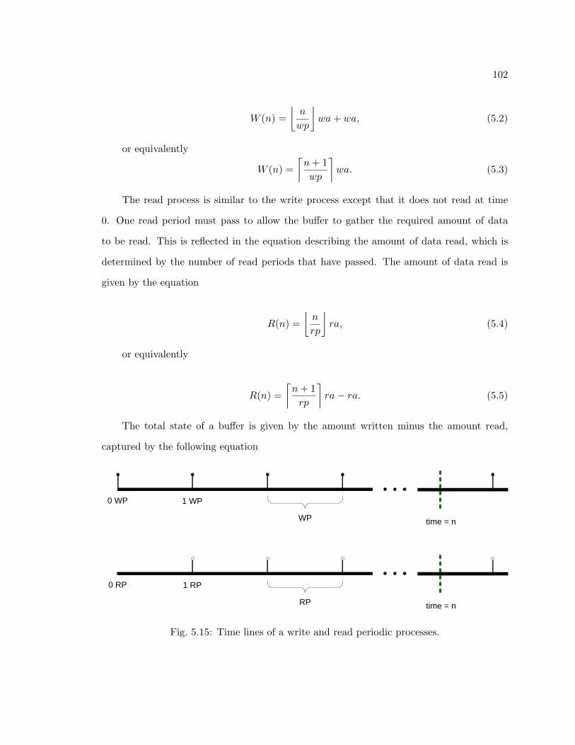
102
W (n) =⌊
n
wp
⌋wa + wa, (5.2)
or equivalently
W (n) =⌈
n + 1wp
⌉wa. (5.3)
The read process is similar to the write process except that it does not read at time
0. One read period must pass to allow the buffer to gather the required amount of data
to be read. This is reflected in the equation describing the amount of data read, which is
determined by the number of read periods that have passed. The amount of data read is
given by the equation
R(n) =⌊
n
rp
⌋ra, (5.4)
or equivalently
R(n) =⌈
n + 1rp
⌉ra− ra. (5.5)
The total state of a buffer is given by the amount written minus the amount read,
captured by the following equation
0 WP 1 WP
WP time = n
0 RP 1 RP
RP time = n
Fig. 5.15: Time lines of a write and read periodic processes.

103
B(n) = W (n) + R(n). (5.6)
By combining (5.2) and (5.4) or combining (5.3) and (5.5), the total state of the buffer
is expressed directly by the equation
B(n) =⌈
n + 1wp
⌉wa−
⌊n
rp
⌋ra. (5.7)
This equation does have one drawback. Time is considered at discrete points, there
are certain values of n in which data is written and also read. The eq. (5.7) only gives the
amount of data in the buffer at the end of time n. In the TOROID telemetry manager, each
buffer is protected so that it is only written to or read from at any given time. Therefore,
there must be an order to the read and write. If the write is first, the buffer will momentarily
contain more data than (5.7) will give. The amount of data that is in the buffer affects the
size the buffer must be to avoid overflowing it.
Using (5.7), the maximum size the buffer will ever be is found by applying the following
ceiling operator property
x ≤ dxe < x + 1. (5.8)
Using (5.8), the amount of data written can be maximized and the amount of data
read can be minimized. The greatest value the write eq. (5.3) can give can be determined
by using the right hand side of (5.8). The smallest value the read eq. (5.8) can give is
determined by using the left hand side of (5.8). This allows the ceiling operators to be
dropped and gives the description of the maximum buffer size as
Bmax =(
n + 1wp
+ 1)
wa−(
n + 1rp
)ra + ra, (5.9)
which expands to
104
Bmax =n + 1wp
wa + wa− n + 1rp
ra + ra, (5.10)
using the relation (5.1)
Bmax =n + 1wp
wa + wa− n + 1wp
wa + ra, (5.11)
simplifies to
Bmax = wa + ra. (5.12)
This relationship matches empirical results found by running extensive simulations of
buffers with varying periods and write and read amounts. The simulations assumed that the
buffer was always written to before read from. This ensured that the simulation was able to
determine the actual maximum amount of data in the buffer. The buffer state repeats itself
due to the periodic nature of the write and read processes. The simulation was run long
enough to capture an entire period so that the true maximum amount the buffer needed
to hold was found. Exact sizes for the telemetry manager are not determined in this thesis
because the required data rates were not known at the time this model was created.
5.4 Conclusion
The approaches of modeling TOROID in SDW differ from each other in level of detail
and modeling focus. The approach of task modeling fails to capture the synchronization
required by the concurrent tasks to enforce their periods. The data modeling fails to capture
a level of detail that yields useful results. The models are either too simplistic or become too
large to create in SDW. These shortcomings lead to an alternative method of representing
data and also interactions between tasks in the telemetry manager. The CSP quantitative
resource models a buffer by representing data as discrete increments. The representation
of time as a global process provides a method to synchronize the concurrent buffers so that
the model represents their behavior correctly. The CSP model of a single buffer shows that

105
the buffer can be written to and read from at different rates. It shows that a balanced
buffer reaches its equilibrium point at which it always has enough data to read and always
has enough space to accept more data for a given set of read and write periods. This single
buffer system can be expanded to model the TOROID telemetry manager that has four
buffers feeding into a single buffer. This model shows if the system will work or not for a
given set of buffer sizes and read and write rates. Mathematical analysis shows the CSP
model to be correct in addition to the formal checks performed by FDR. The mathematical
method gives a way to show correctness when the model becomes to large to be able to
model.

106
Chapter 6
Conclusion
The tool development presented in this thesis gives greater ability to characterize sys-
tems formally and perform mathematically based analysis.
There has been much research done on how to model systems using a variety of ap-
proaches. Some of the methods have been more general and others are targeted for a specific
domain. Different graphical techniques have also been applied in order to facilitate the use
of more difficult and obscure formal methods and make them more available for designers
and engineers to use. Formal methods have proven themselves in being useful to reduce
costly design flaws and produce more reliable systems. Software that is modeled can be un-
derstood better and also checked for obscure errors that are difficult to find using standard
testing methods. Software that is modeled can be understood better and also checked for
obscure errors that are difficult to find using standard testing methods.
The Spacecraft Design Workbench is a graphical modeling tool that has been targeted
at describing spacecraft behavior combining two different types of design tools, FFBDs and
DFDs. Using these two tools, an interface is given to the user that allows the detailed
description of systems. Since a graphical design is difficult to formally verify, an important
key is being able to traverse the graphical design and generate a corresponding model in
a language that has a solid mathematical foundation. The generated model can then be
checked automatically to verify the model for specific design requirements.
By adding constraints to the SDW tool, the user has more power to describe different
systems that can be translated to CSP for analysis. The addition of the between and outside
constraint gives more power to the graphical modeling capability and more closely matches
the formal CSP framework developed by McInnes.
In order to create a model that is meaningful, the correct tool for the desired system

107
must be used. The tool must be able to capture the meaningful aspects of the system
that allows the asking of meaningful questions. SDW was created to be able to describe
a system at the system level. This enables SDW to capture the systems behavior by
observing subsystem interactions. In describing the telemetry manager, this tool becomes
less descriptive because it does not allow the asking of meaningful questions. Though the
telemetry manager has many different concurrently running parts, SDW is unable to capture
the relationship they have to each other in a practical way that enables designers to know if
the buffer interaction will be correct. This is due to the exact periodic nature of the buffers
and the difficulty in enforcing correct behavior in SDW.
With additional tools that are designed to handle periodic tasks, the description of the
telemetry manager for TOROID becomes more meaningful. The CSP timer process allows a
task whose correct function depends on running at the correct rate relative to one or more
tasks. Since the buffer system is the main critical component in the telemetry manager
system, being able to describe it formally is vital in order to be able to ask any meaningful
questions. The main question is whether or not the buffers are each large enough so that
the different rates of reading and writing to them does not allow the buffer to overflow
or underflow. Being able to simulate this system formally gives detailed insight into the
behavior of the multiple buffers.
Combining formal model checking with a mathematical analysis allows the system to
be designed to pass the formal model checking and removes the guess and check tweaking
of the system. The mathematical description that allows a prediction to be made about the
system working correctly makes it simpler for the designer to build it correctly. The formal
analysis show that the system does indeed do what it was intended to do and verifies the
correct function by rigorously testing it.
Another project that is related to this thesis and is currently underway at USU includes
creating a graphical front end for the remaining CSP behavior processes developed by
McInnes. This work is being done as another master’s thesis. It is creating a tool that is
even more domain specific than SDW in that the constructs supported are directly focused,

108
enabling a more intuitive description of a satellite by giving pre-specified constructs common
to satellite systems. This work will further extend the capability of spacecraft designers by
giving them a tool that has formal analysis capability and support.
Possible future work extending this thesis could involve allowing the read and write
processes of the buffer to start and stop at different times. This could allow data collection
to start well before the data is formatted into a specific downlink format or allow a slower
read process to continue emptying a buffer after the writing has stopped. This could also
be applied to describe ground testing of instruments that produce high volumes of data in
short amounts of time where the data must be collected rapidly and then processed and
moved to a higher storage device.
109
References
[1] A. I. S. McInnes, A Formal Approach to Specifying and Verifying Spacecraft Behavior.Ph.D. dissertation, Utah State University, Logan, UT, 2007.
[2] J. C. M. Baeten, “A brief history of process algebra,” Theoretical Computer Science,vol. 335, no. 2-3, pp. 131–146, 2005.
[3] G. H. Hilderink, “Graphical modelling language for specifying concurrency based onCSP,” in Proceedings of IEE Software, pp. 108–120, Apr. 2003.
[4] F. Scuglik and M. Sveda, “Automatically generated csp specifications,” Journal ofUniversal Computer Science, vol. 9, no. 11, pp. 1277–1295, Nov. 2003, http://www.jucs.org/jucs_9_11/automatically_generated_csp_specifications.
[5] J. Long, “Relationships between common graphical representations in system engi-neering,” Vitech white paper, Aug. 2002, http://www.vitechcorp.com/whitepapers/files/200701031634430.CommonGraphicalRepresentations_2002.pdf.
[6] S. Wall, “Model-based engineering design for space missions,” in Proceedings of IEEEAerospace Conference, pp. 3907–3915, Mar. 2004.
[7] M. Chechik and A. Wong, “Formal modeling in a commercial setting: a case study,”Journal of Systems and Software, vol. 60, no. 1, pp. 59–82, 2002.
[8] K. Havelund, M. Lowry, and J. Penix, “Formal analysis of a space-craft controller usingspin,” IEEE Transactions on Software Engineering, vol. 27, no. 8, pp. 749–765, Aug.2001.
[9] A. McInnes, B. Eames, and R. Grover, “Formalizing functional flow block diagramsusing process algebra and metamodels,” IEEE Transactions on System, Man and Cy-bernetics, Part A, to appear.
[10] J. E. Crace, “Toroid software subsystem,” Master’s thesis, Utah State University, Lo-gan, UT, 2007.
[11] J. D. Jensen, “The design of the command and data handling sub-system used by theionospheric observation nano-satellite formation,” Master’s thesis, Utah State Univer-sity, Logan, UT, 2000.
[12] Wind River Systems, Inc, “Vxworks programmer’s guide,” 1997, part Number DOC-12067-ZD-00.
[13] B. K. Eames, A. I. McInnes, J. E. Crace, and J. M. Graham, “A model-based design toolfor systems-level spacecraft design,” in Proceedings American Institute of Aeronauticsand Astronautics/Utah State University Conference on Small Satellites, Aug. 2006.
110
[14] A. Roscoe, The Theory and Practice of Concurrency. Englewood Cliffs, NJ: PrenticeHall, 2005.
[15] S. Schneider, Concurrent and Real-time Systems The CSP Approach. EnglewoodCliffs, NJ: John Wiley & Sons, 2000.
[16] D. W. Oliver, T. P. Kelliher, and J. James G. Keegan, Engineering Complex Systemswith Models and Objects. Columbus, OH: McGraw-Hill, 1997.
[17] A. Bahill, M. Alford, K. Bharathan, J. Clymer, D. Dean, J. Duke, G. Hill, E. LaBudde,E. Taipale, and A. Wymore, “The design-methods comparison project,” IEEE Trans-actions on Systems, Man, and Cybernetics, Part C: Applications and Reviews, vol. 28,no. 1, pp. 80–103, Feb. 1998.

111
Appendices
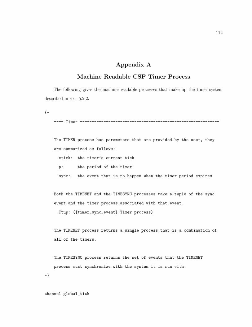
112
Appendix A
Machine Readable CSP Timer Process
The following gives the machine readable processes that make up the timer system
described in sec. 5.2.2.
{-
---- Timer -----------------------------------------------------------
The TIMER process has parameters that are provided by the user, they
are summarized as follows:
ctick: the timer’s current tick
p: the period of the timer
sync: the event that is to happen when the timer period expires
Both the TIMENET and the TIMESYNC processes take a tuple of the sync
event and the timer process associated with that event.
Ttup: ({timer_sync_event},Timer process)
The TIMENET process returns a single process that is a combination of
all of the timers.
The TIMESYNC process returns the set of events that the TIMENET
process must synchronize with the system it is run with.
-}
channel global_tick
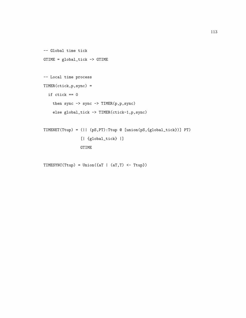
113
-- Global time tick
GTIME = global_tick -> GTIME
-- Local time process
TIMER(ctick,p,sync) =
if ctick == 0
then sync -> sync -> TIMER(p,p,sync)
else global_tick -> TIMER(ctick-1,p,sync)
TIMENET(Ttup) = (|| (pS,PT):Ttup @ [union(pS,{global_tick})] PT)
[| {global_tick} |]
GTIME
TIMESYNC(Ttup) = Union({aT | (aT,T) <- Ttup})

114
Appendix B
Machine Readable CSP Telemetry Manager
This model of the telemetry manager has four source buffers that are read by the
periodic telemetry manager. The telemetry manager builds a page at a time in this model,
when eight pages have been built, the data is read from the telemetry buffer and the process
repeats. This model shows the idea of how the telemetry manager works, but due to scaling
challenges must be simplified, so the amounts of data written and read from the buffer must
be scaled down. The quantitative resource process is from A Formal Approach to Specifying
and Verifying Spacecraft Behavior [1].
-- Timer process parameters
-- QR buffer parameters
-- image buffer
imgWP = 600
imgWA = 600
imgRA = -48
imgMAX = 648
imgMIN = 0
imgINIT = 0
-- sci 1 buffer
sci1WP = 48
sci1WA = 48
sci1RA = -48
sci1MAX = 96
sci1MIN = 0

115
sci1INIT = 0
-- sci 2 buffer
sci2WP = 96
sci2WA = 96
sci2RA = -48
sci2MAX = 144
sci2MIN = 0
sci2INIT = 0
-- sci 3 buffer
sci3WP = 2
sci3WA = 2
sci3RA = -48
sci3MAX = 50
sci3MIN = 0
sci3INIT = 0
-- tel buffer
telWP = 48
telWA = 1
telRP = 384
telRA = -8
telOffset = 48
telMAX = 392
telMIN = 0
telINIT = 0

116
-- QR channels
channel imgIO:{ -imgMAX..imgMAX}
channel imgRead,imgTrans: {imgMIN..imgMAX}
channel sci1IO:{ -sci1MAX..sci1MAX}
channel sci1Read,sci1Trans: {sci1MIN..sci1MAX}
channel sci2IO:{ -sci2MAX..sci2MAX}
channel sci2Read,sci2Trans: {sci2MIN..sci2MAX}
channel sci3IO:{ -sci3MAX..sci3MAX}
channel sci3Read,sci3Trans: {sci3MIN..sci3MAX}
channel telIO:{ -telMAX..telMAX}
channel telRead,telTrans: {telMIN..telMAX}
-- Time Sync events
channel imgTimeWrite, sci1TimeWrite, sci2TimeWrite, sci3TimeWrite
channel telTimeWrite,telTimeRead
-- Buffer write/read processes
imgWrite = imgTimeWrite -> imgIO!imgWA -> imgTimeWrite ->
imgWrite
sci1Write = sci1TimeWrite -> sci1IO!sci1WA -> sci1TimeWrite ->
sci1Write
sci2Write = sci2TimeWrite -> sci2IO!sci2WA -> sci2TimeWrite ->
sci2Write
sci3Write = sci3TimeWrite -> sci3IO!sci3WA -> sci3TimeWrite ->
sci3Write
telWrite = telTimeWrite -> imgIO!imgRA -> sci1IO!sci1RA ->
sci2IO!sci2RA -> sci3IO!sci3RA -> telIO!telWA ->
telTimeWrite -> telWrite

117
TELRead = telTimeRead -> telIO!telRA -> telTimeRead -> TELRead
imgQR = QuantResource(imgIO,imgRead,imgTrans,imgMIN,imgMAX,imgINIT)
sci1QR = QuantResource(sci1IO,sci1Read,sci1Trans,sci1MIN,sci1MAX,sci1INIT)
sci2QR = QuantResource(sci2IO,sci2Read,sci2Trans,sci2MIN,sci2MAX,sci2INIT)
sci3QR = QuantResource(sci3IO,sci3Read,sci3Trans,sci3MIN,sci3MAX,sci3INIT)
telQR = QuantResource(telIO,telRead,telTrans,telMIN,telMAX,telINIT)
imgTW = TIMER(0,imgWP,imgTimeWrite)
sci1TW = TIMER(0,sci1WP,sci1TimeWrite)
sci2TW = TIMER(0,sci2WP,sci2TimeWrite)
sci3TW = TIMER(0,sci3WP,sci3TimeWrite)
telTW = TIMER(telWP,telWP,telTimeWrite)
telTR = TIMER(telRP+telWP,telRP,telTimeRead)
-- IMG tests
alpImg = {({imgTimeWrite},imgTW),
({telTimeWrite},telTW)}
imgTNET = TIMENET(alpImg)
aImgTnet = TIMESYNC(alpImg)
imgSYS = ((imgWrite ||| telWrite)
[|{|imgIO|}|] imgQR)
[| aImgTnet |] imgTNET
assert imgSYS :[deadlock free [F]]

118
assert imgSYS :[deadlock free [FD]]
-- SCI1 tests
alpSci1 = {({sci1TimeWrite},sci1TW),
({telTimeWrite},telTW)}
sci1TNET = TIMENET(alpSci1)
aSci1Tnet = TIMESYNC(alpSci1)
sci1SYS = ((sci1Write ||| telWrite)
[|{|sci1IO|}|] sci1QR)
[| aSci1Tnet |] sci1TNET
assert sci1SYS :[deadlock free [F]]
assert sci1SYS :[deadlock free [FD]]
-- SCI2 tests
alpSci2 = {({sci2TimeWrite},sci2TW),
({telTimeWrite},telTW)}
sci2TNET = TIMENET(alpSci2)
aSci2Tnet = TIMESYNC(alpSci2)
sci2SYS = ((sci2Write ||| telWrite)
[|{|sci2IO|}|] sci2QR)
[| aSci2Tnet |] sci2TNET
assert sci2SYS :[deadlock free [F]]

119
assert sci2SYS :[deadlock free [FD]]
-- SCI3 tests
alpSci3 = {({sci3TimeWrite},sci3TW),
({telTimeWrite},telTW)}
sci3TNET = TIMENET(alpSci3)
aSci3Tnet = TIMESYNC(alpSci3)
sci3SYS = ((sci3Write ||| telWrite)
[|{|sci3IO|}|] sci3QR)
[| aSci3Tnet |] sci3TNET
assert sci3SYS :[deadlock free [F]]
assert sci3SYS :[deadlock free [FD]]
-- TEL tests
alpTel = {({telTimeWrite},telTW),
({telTimeRead},telTR)}
telTNET = TIMENET(alpTel)
aTelTnet = TIMESYNC(alpTel)
telSYS = ((telWrite ||| TELRead)
[|{|telIO|}|] telQR)
[| aTelTnet |] telTNET
assert telSYS :[deadlock free [F]]
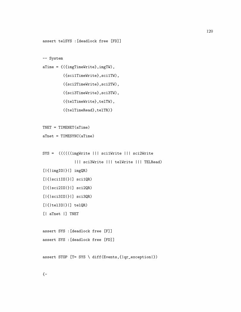
120
assert telSYS :[deadlock free [FD]]
-- System
aTime = {({imgTimeWrite},imgTW),
({sci1TimeWrite},sci1TW),
({sci2TimeWrite},sci2TW),
({sci3TimeWrite},sci3TW),
({telTimeWrite},telTW),
({telTimeRead},telTR)}
TNET = TIMENET(aTime)
aTnet = TIMESYNC(aTime)
SYS = ((((((imgWrite ||| sci1Write ||| sci2Write
||| sci3Write ||| telWrite ||| TELRead)
[|{|imgIO|}|] imgQR)
[|{|sci1IO|}|] sci1QR)
[|{|sci2IO|}|] sci2QR)
[|{|sci3IO|}|] sci3QR)
[|{|telIO|}|] telQR)
[| aTnet |] TNET
assert SYS :[deadlock free [F]]
assert SYS :[deadlock free [FD]]
assert STOP [T= SYS \ diff(Events,{|qr_exception|})
{-

121
---- Timer -----------------------------------------------------------
-}
channel global_tick
-- Global time tick
GTIME = global_tick -> GTIME
-- Local time process
TIMER(SCBF_ctick,SCBF_p,SCBF_sync) =
if SCBF_ctick == 0
then SCBF_sync -> SCBF_sync -> TIMER(SCBF_p,SCBF_p,SCBF_sync)
else global_tick -> TIMER(SCBF_ctick-1,SCBF_p,SCBF_sync)
TIMENET(SCBF_Ttup) = (|| (pS,PT):SCBF_Ttup @ [union(pS,{global_tick})] PT)
[| {global_tick} |]
GTIME
TIMESYNC(SCBF_Ttup) = Union({aT | (aT,T) <- SCBF_Ttup})
{-
---- Quantitative Resource -------------------------------------------
__QuantResource__ is a process encapsulating an integer quantitative
value (’val’). This value has upper and lower bounds ’max’ and ’min’.
The value can be changed by sending an integer-valued magnitude of
change through channel ’delta’, and read through channel ’get’.
Changes in the value result in a signal on channel ’trans’.
The initial value of ’val’ is ’init’. Changes in the value that
result in ’val’ exceeding the upper or lower bounds result in a

122
corresponding signal on channel ’qr_exception’ and termination of
the process.
-}
datatype ResourceException = resource_overflow | resource_underflow
channel qr_exception : ResourceException
QuantResource(SCBF_delta, SCBF_get, SCBF_trans,
SCBF_min, SCBF_max, SCBF_init) =
let
Range = {SCBF_min..SCBF_max}
Quantity(val) =
val > SCBF_max & qr_exception.resource_overflow -> STOP
[]
val < SCBF_min & qr_exception.resource_underflow -> STOP
[]
member(val, Range) & (SCBF_get!val -> Quantity(val))
[]
member(val, Range) &
(SCBF_delta?d ->
let
val’ = val + d
within
if (val’ != val) and member(val’, Range)
then (SCBF_trans!val’ -> Quantity(val’))
else Quantity(val’))
within
Quantity(SCBF_init)