an exploration of automotive platinum demand and its
TRANSCRIPT

An Exploration of Automotive Platinum Demandand its Impacts on the Platinum Market
by
Christopher George Whitfield ARCHES
Submitted to the Department of Materials Science and Engineeringin Partial Fulfillment of the Requirements for the Degree of
Bachelor of Science
at the
Massachusetts Institute of Technology
May 2009E 4n e 2 4
MASSACHUS. -S INSTUTEOFTECHNOLOGY
FEB 0 8 2010
LIBRARIES
C 2009 Christopher Whitfield All rights reservedThe author hereby grants to MIT permission to reproduce and to distribute publicly paper and
electronic copies of this thesis document in whole or in part in any medium now known or hereaftercreated.
Signature of A uthor .................................................. .. ....... ..... ....................... ..............Department of M terials Science and Engineering
S / . / // / jlMay)2, 2009
Certified by ..................................... ........../ / Randolph kirchain Jr.
Assistant Professor of Materials Science and EngineeringThesis Supervisor
Accepted by..................................... . -.........A c c e p t e d b y ....................................................................................... . L i o n e l C.. . . . . . . .m e .li n.Lionel C. Kimerling
Professor of Materials Science and EngineeringChair, Undergraduate Committee

An Exploration of Automotive Platinum Demandand the Impacts on the Platinum Market
by
Christopher George Whitfield
Submitted to the Department of Materials Science and Engineeringon May 12, 2009
in Partial Fulfillment of the Requirements for the Degree ofBachelor of Science
Abstract
The platinum market is a material market of increasing interest, as platinum demand has grownfaster than supply in recent years. As a result, the price of platinum has increased, causing end-userfirms to experience material scarcity through the presence of these high prices. A significant driverof this demand growth for the last several decades is demand automotive sector, which isresponsible for almost 60% of total primary platinum demand, due to the use of platinum in threeway catalysts. Platinum is one of the materials utilized to catalyze reactions that prevent vehicleemissions from entering the atmosphere, which can have a severe impact on air quality. Two factorswill likely contribute to the future growth of automotive platinum demand: the trend in increaseduse of platinum per vehicle, and expected growth in the number of automobiles produced and soldaround the world. While the automotive market is relatively saturated in developed economies,automotive sales growth potential is particularly high in developing areas, such as BRIC countries. Itfollows that future growth in automotive platinum demand is likely to be significant. As such, thestudy aims to characterize the drivers of automotive platinum demand and to establish how thisdemand sector impacts the platinum market as a whole. This characterization is achieved throughregression analysis and by utilizing a platinum market simulation model. The regression resultsindicate that the automotive platinum demand has historically been an inelastic one. Globalautomotive sales have indeed been a driver of platinum demand behavior. Regression on automotivesales in India, a BRIC country has high correlation with wealth as measured by GDP per capita. Inthe US and Japan, automotive sales show high autocorrelation and additional correlativerelationships were not confirmed. Model results show that the automotive industry drives platinumprice increases when there is a combination of low elasticity of platinum demand and large growthrates in the global automotive industry. Recent news about new technologies suggests that demandelasticity may increase, and the model suggests that higher elasticity would reduce the impact ofautomotive industry growth on the total demand for platinum.

Contents
LIST OF FIGURES .............................................................................................................. 5
LIST OF TABLES ........... ........................................................................................ 7
ACKNOW LEDGEM ENTS.................................................. ........................................ 8
I. INTRODUCTION .................................................................................................. 9
A. Motivation & Background .......................................... ........... 9
B. Problem Statement ..................................................... 16
II. M ETH ODOLOGY ...................................................................................................... 16
A. Regression Analysis Methodology...................................................................................................................... 16
B. Platinum Market Simulation Model Methodology ..................................................... 18
III. UNDERSTANDING AUTOMOTIVE PLATINUM DEMAND........................... 18
A. Automotive Demand Factors ..................................................................................................................................... 18
IV. REGRESSION RESULTS......................................... ........... ................................. 21
A. Why Regression? ....................................................................................................................................................... 21
B. Global Automotive Sales Relationships .................................................................................................................... 21
C. Global Automotive Platinum Demand Relationships .................................................................................... 25
D. Country Specific Automotive Sales Relationships ................................................................................................. 27
E. Country Specific Platinum Demand Relationships ........................................................................................ 29
F. Comparison to Palladium Dynamics ................................................................................................................. 30
G. Regression Analysis Discussion and Conclusions .......................................................................................... 31
V. PLATINUM MARKET SIMULATION MODEL RESULTS ................................... 32
A. Model Structure and Base Case Behavior ................................................................................................................ 32
B. Exogenous Variable Sensitivity Analysis ......... ............................................................ 39

1. L ow E lasticity ................................................................................................................................................................................... 44 12. Medium and High Elasticity ......................................................................................................................................................... 462. Medium and High Elasticit.....
C. Platinum Market Simulation Model Conclusions .................................................................................................. 55
VI. FUTURE W ORK........................................................................................................ 58
VII. BIBLIOGRAPHY....................................................................................................... 59

List of Figures
Figure 1 Platinum demand aggregated by: total global usage, total global automotive usage, and total
N orth Am erican automotive usage [12]. .................................................................................................. 10
Figure 2 Basic oxidation and reduction reactions desired in three-way catalysts [5]......................... 11
Figure 3 Inflation-adjusted teal price of platinum in 2000 USD from 1975 to 2007[7]......... . 13
Figure 4 Vehicles per Thousand People: U.S. (Over Time) Compared to Other Countries (in 1996
and 2006) [9] ....................................................................... 15
Figure 5: Percentage of platinum and palladium per vehicle from 1980 to 2004 and total platinum
and palladium per vehicle (in grams) from 1980 to 2004 [3] ..................................... ...... 20
Figure 6 Example trend-line fitting performed in Excel. On the left, total global automotive
production versus global GDP per capita; on the right, versus total global population .......... 22
Figure 7: Schematic of the platinum market simulation model [17]............................... ........ 34
Figure 8 Gross platinum demand, stacked by industry, over 60-year time horizon................ 36
Figure 9 Sales recycling by industry, base case, 60 year horizon............................................... 37
Figure 10 Primary purchase of platinum by industry, base case, 60 year horizon .............................. 37
Figure 11 Automotive industry primary versus recycled platinum use by percentage, base case, 60
year horizon ...................................................................................................................................................... 38
Figure 12 Price of platinum over 60-year time horizon .................................... .... .............. 39
Figure 13 Automotive sector gross platinum demand, base case elasticity, varying growth........... 42
Figure 14 Total platinum gross demand average and standard deviations (regular and normalized),base case elasticity, varying growth. ........................................ ...................................................... 43
Figure 15 Platinum price, average and standard deviation (regular and normalized), base case
elasticity, varying growth.................................................. 45
Figure 16 Average automotive platinum gross demand at three levels of elasticity, varying
automotive platinum demand growth rates.................................................................................... 48
Figure 17 Normalized standard deviation of automotive platinum gross demand at three levels of
elasticity, varying automotive platinum demand growth rates............................... ........ 48
Figure 18 Average total platinum demand at three levels of elasticity, varying automotive platinum
demand growth rates . ...................................................... 50
Figure 19 Normalized standard deviation of total platinum demand at three levels of elasticity,varying automotive platinum demand growth rates ......................................... ............ 51

Figure 20 Average platinum price at three levels of elasticity, varying automotive platinum demandgrowth rates. Outliers excluded from analysis include a peak price of 334.9 for the lowelasticity scen ario ............................................................................................................................................ 5 2
Figure 21 Normalized standard deviation of platinum price at three levels of elasticity, varyingautomotive platinum demand growth rates...................................................................................... 53
Figure 22 Platinum price over time at three levels of elasticity, 60 year time horizon ...................... 55

List of Tables
Table 1 Results from Excel trend line fitting for various automotive data ..................................... 22
Table 2 STATA regression results for platinum price and world total automotive sales ..................... 22
Table 3 STATA regression results for automotive demand and automotive platinum demand........ 23
Table 4 STATA regression results for automotive palladium demand.............................. ...... 31
Table 5 Analysis scenarios examining demand elasticity and demand growth .................................... 41

Acknowledgements
First off, I am thankful for the opportunity to perform my undergraduate thesis research under
Professor Randy Kirchain, as it allowed me to pursue a thesis topic that was engaging and in line
with my interests. The entire research project would not have been possible, however, without thehelp of Elisa Alonso. Her patience, perspective, and guidance helped direct my research for the last
six months, and I cannot express how appreciative I am of her support along the way. I am perhapsmost thankful for the unwavering support that my family has shown me throughout the years,including my wonderful parents; my brothers Richard and David; my sister Kathleen; my sister-in-law Lindsay; and of course my beautiful goddaughter Chloe Violet. I also cannot be thankfulenough for the constant support and encouragement provided by Jenny over the course of the year.Finally, I would like to thank my friends, especially my fraternity Brothers, and all of those whom I
have had the honor of meeting during my time at MIT, for making this the experience of a lifetime.
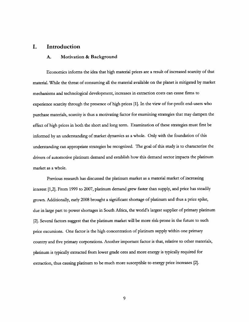
I. Introduction
A. Motivation & Background
Economics informs the idea that high material prices are a result of increased scarcity of that
material. While the threat of consuming all the material available on the planet is mitigated by market
mechanisms and technological development, increases in extraction costs can cause firms to
experience scarcity through the presence of high prices [1]. In the view of for-profit end-users who
purchase materials, scarcity is thus a motivating factor for examining strategies that may dampen the
effect of high prices in both the short and long term. Examination of these strategies must first be
informed by an understanding of market dynamics as a whole. Only with the foundation of this
understanding can appropriate strategies be recognized. The goal of this study is to characterize the
drivers of automotive platinum demand and establish how this demand sector impacts the platinum
market as a whole.
Previous research has discussed the platinum market as a material market of increasing
interest [1,2]. From 1999 to 2007, platinum demand grew faster than supply, and price has steadily
grown. Additionally, early 2008 brought a significant shortage of platinum and thus a price spike,
due in large part to power shortages in South Africa, the world's largest supplier of primary platinum
[2]. Several factors suggest that the platinum market will be more risk-prone in the future to such
price excursions. One factor is the high concentration of platinum supply within one primary
country and five primary corporations. Another important factor is that, relative to other materials,
platinum is typically extracted from lower grade ores and more energy is typically required for
extraction, thus causing platinum to be much more susceptible to energy price increases [2].

7000
6000
40 ----- World Auto Pt Usa0" -- Total World Pt Usage
. N.A. Auto Pt Usage
2000
1000
1975 1980 1985 1990 1995 2000 2005 2010
Year
Figure 1 Platinum demand aggregated by: total global usage, total global automotive usage, andtotal North American automotive usage [12].
An additional factor to be considered with regard to platinum demand is the significant
amount of platinum used in automobile catalysts, which accounted for almost 60% of total global
platinum primary demand in 2007 [3]. The significant growth rate of automotive platinum usage can
be seen in Figure 1. The origination of catalyst use in the United States and thus the origin of
significant demand for platinum from this sector is an interesting history and one that is important
to understand, given that other countries have or may in the future follow a similar trend in policy
and technology choices.
Air pollution became a central topic of interest in the U.S. in the mid 20' century as air
quality in urban areas worsened, mainly due to the increased numbers of vehicles on the road.
Emissions standards developed as a reaction to this air deterioration, established first at the State
level and eventually, in 1967, established by the Federal Government through the Air Quality Act
[4]. The main function of this act was to exert federal control over emissions standards, as this
10

control had previously been a point of debate. This set the stage for the defining legislation in this
area with the 1970 Clean Air Act.
The requirements of the legislation were aggressive: car companies were required to make
90 percent reductions in unburned hydrocarbons (HC) and carbon monoxide (CO) for model year
1975 vehicles, and 90 percent reductions in nitrogen oxides (NOx) for model year 1976. To meet
these standards, which would in reality evolve over the next several years given technological
limitations, the auto companies adopted the catalytic converter in 1975. This first generation
technology did little to help reduce NOx emissions, and was thus replaced in 1981 by the three-way
catalyst (TWC), the catalyst installed in many vehicles today.
Understanding the technology behind TWCs helps to explain why the utilization of these
elements led to a significant increase in platinum demand. The basic reaction occurring in a typical
internal combustion engine is the combustion of gasoline. However, this combustion is not
complete, thus there are byproducts of the reaction emitted through the exhaust, including benign
elements as well as three major pollutants: CO, HC, and NOx. TWCs are intended to prevent large
portions of these pollutants from entering the atmosphere [5].
TWC's eliminate the pollutants in the exhaust through a combination of oxidation/reduction
reactions. For CO and HC, these are oxidation reactions, and for NOx, it is a reduction reaction.
Heck & Farrauto have captured these basic chemical reactions:
NO (or NO) + CO -* N2 + CO2
CH+ I + O YCO + -H20yH + yO2 NO (or NO2) + H2 - N2 + H2
CO + 02 -+ CO2 2 + ) NO (or NO2 ) + C,H.
CO +H2O- CO +2 - + N, + yCO2 + H20
Figure 2 Basic oxidation and reduction reactions desired in three-way catalysts [5].

These reactions occur in a more thermally efficient manner in the presence of a catalyst.
Even with a catalyst, the reactions require some heat and therefore the TWC uses heat from the
gasoline combustion reaction that is transferred to the catalyst through the exhaust system. Once
the required level of heat for any given reaction is reached on the surface of the catalyst, the reaction
will proceed and eliminate much of the pollutant from the exhaust [5].
Understanding why precious metals are selected to catalyze these reactions is important, and
Shelef and McCabe provide justification for this choice [6]. First, the catalytic activity of precious
metals is significantly higher than most other options, which is particularly important considering the
high speed at which the reactions must occur-since the flow rate of exhaust determines how
quickly pollutants must be eliminated-as well as the required size of the catalyst, in terms of
practical application to vehicles. Secondly, sulfur oxides in the exhaust have the potential to poison
many possible catalytic materials, with precious metals being an exception. Finally, precious metals
are, for the most part, immune to deactivation caused by interactions with "the insulator oxides of
Al, Ce, Zr, etc., which constitute the so-called high surface area "washcoat" on which the active
catalytic components are dispersed" [6].
Since the development of the TWC, platinum group metals (PGMs) have been utilized as
catalysts. Originally, platinum and palladium were used in catalysts, with the adoption of rhodium
coming only after regulations surrounding NOx emissions were tightened, as rhodium is a
particularly effective reducing agent for nitrogen oxides [6]. Platinum and rhodium were, at the
advent of the increased demand for PGMs, significantly more expensive than palladium; however,
palladium was not utilized more widely because of its sensitivity to lead poisoning. Only as the lead
content of gasoline dropped throughout the 70s and 80s did palladium not only became a viable
substitute for platinum and rhodium, but one that was heavily utilized beginning in 1989. It is

important to recognize that palladium use in catalysts hinges on the availability of unleaded gasoline
for the vehicles utilizing the technology, and thus is not a perfect substitute in all countries or
regions. Evidently, adoption of TWCs has led to an increased demand for all PGMs for use as
catalysts, with platinum being no exception.
Examining the link between these policy and technology choices and the price of platinum
highlights their impact on the overall platinum market. The impact of this new demand is most
evidently illustrated by the trend in the price of platinum, which spiked significantly in the years
following the establishment of this new automotive platinum demand sector: While this price
increase was partially offset soon thereafter, the real price did not return to its pre-1980 levels until
recently, suggesting a permanent impact on the price of platinum and thus on the platinum market,
the details of which will be expanded upon [Figure 3].
45
40
i 35
2 2
S20...........
10
1975 1980 1985 1990 1995 2000 2005 2010
Time (years)
Figure 3 Inflation-adjusted teal price of platinum in 2000 USD from 1975 to 2007[7].
A simplified view of the world, broken down into developed and developing economies,
allows assumptions about future vehicle demand to be made concerning each. While developed

economies, such as the U.S. and Japan, are more saturated with regard to the vehicle market,
developing economies are far behind by this metric. This dichotomy is captured in Figure 4.
Clearly, if the rate at which the U.S. has ascended in terms of vehicles per capita is any indication,
expectations for future automobile sales in developing economies should be significant. Indeed, to
capture the true magnitude of this potential ascension to the current U.S. ratio of over 800 vehicles
per 1000 people, consider that both Asia, which includes India, and China currently possess around
50 vehicles per 1000 people. If India and China attained a level of even 250 vehicles per 1000
people - a level attained by the U.S. in the1940s - this would require almost 500 million vehicles to
be sold in these countries, and only if population were constant. Considering that the number of
vehicles in the world currently stands at around 900 million, this would be an increase of well over
50% solely from the growth of two countries [8].

250
* 200
100
* 00
i Goo30
200
100
0
Eastem Europe 2006
U.S
Eastern Europe 1996
Cerral & South America 2006
Cedral & South America 1996MLdde East 2006
Asia 2006 Mdde East 1996Asia 1996
ChNa 2006MAlIca 1996 & 2006
ChM 1996
1900 1905 1910 1915 1920 1925 1930 1935 1940
U.S
Canada 1996
PacI fc 2006P~W eW Europe 1996
See facing page
II1 11 111 11 111 11 111 11 11T 11'11111T 11T1T!T 1 T 111'TITI 11111111filf lTI l illllll lll lll I IIIIII II{']
1900 19910 1920 1930 1940 1950 1960 1970 190 1990 2000
Figure 4 Vehicles per Thousand People: U.S. (Over Time) Compared to Other Countries(in 1996 and 2006) [9]

A potential trend, which is of importance due to the significant portion of platinum demand
accounted for by the automotive sector, is the increased demand for automobiles in these
developing countries. This trend will likely be realized, as evident market potential and recent news
developments suggest [10]. Additionally, platinum demand has historically been driven by
automotive sales due to the use of platinum in TWCs. The remaining factor is defining the strength
of the link between these trends in developing economies; that is, what the current state of TWC
utilization in these economies is, and thus how much platinum is used. With regard to official
policies, China, India, and Brazil, in addition to many other developing countries, have passed
emission standards requiring the reduction of HC, CO, and NOx emissions from vehicles,
presumably through the utilization of TWCs. The adherence to these policies may be another
question altogether in these countries, and thus the assumption that a TWC is included with every
vehicle may be erroneous, though for now this assumption will be accepted.
B. Problem Statement
The goal of this study is to characterize the drivers behind automotive platinum demand and
establish how this demand sector impacts the platinum market as a whole.
II. Methodology
A. Regression Analysis Methodology
To define the impact of the automotive demand sector on the platinum market, statistical
analysis on several variables was performed. Analysis of these relationships was initially examined
utilizing trend-line fitting in Microsoft Excel, which in the case of linear relationships defined the
slope of the line relating the two variables, and also provided an estimate of the determination
16
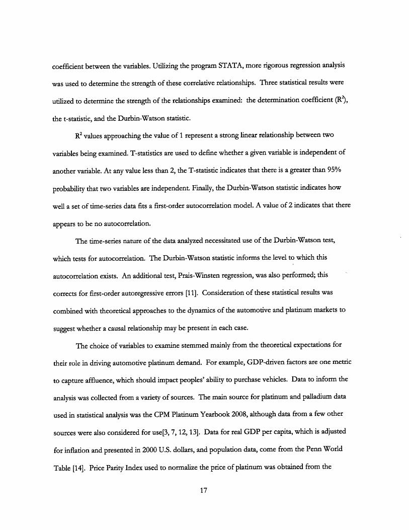
coefficient between the variables. Utilizing the program STATA, more rigorous regression analysis
was used to determine the strength of these correlative relationships. Three statistical results were
utilized to determine the strength of the relationships examined: the determination coefficient (R),
the t-statistic, and the Durbin-Watson statistic.
R2 values approaching the value of 1 represent a strong linear relationship between two
variables being examined. T-statistics are used to define whether a given variable is independent of
another variable. At any value less than 2, the T-statistic indicates that there is a greater than 95%
probability that two variables are independent. Finally, the Durbin-Watson statistic indicates how
well a set of time-series data fits a first-order autocorrelation model. A value of 2 indicates that there
appears to be no autocorrelation.
The time-series nature of the data analyzed necessitated use of the Durbin-Watson test,
which tests for autocorrelation. The Durbin-Watson statistic informs the level to which this
autocorrelation exists. An additional test, Prais-Winsten regression, was also performed; this
corrects for first-order autoregressive errors [11]. Consideration of these statistical results was
combined with theoretical approaches to the dynamics of the automotive and platinum markets to
suggest whether a causal relationship may be present in each case.
The choice of variables to examine stemmed mainly from the theoretical expectations for
their role in driving automotive platinum demand. For example, GDP-driven factors are one metric
to capture affluence, which should impact peoples' ability to purchase vehicles. Data to inform the
analysis was collected from a variety of sources. The main source for platinum and palladium data
used in statistical analysis was the CPM Platinum Yearbook 2008, although data from a few other
sources were also considered for use[3, 7, 12, 13]. Data for real GDP per capita, which is adjusted
for inflation and presented in 2000 U.S. dollars, and population data, come from the Penn World
Table [14]. Price Parity Index used to normalize the price of platinum was obtained from the

Bureau of Labor Statistics [15]. All vehicle data was taken from Ward's Motor Vehicle Data 2007
[8].
B. Platinum Market Simulation Model Methodology
Examination of the impact of automotive demand for platinum on the overall platinum
market was achieved through the use of a platinum market simulation model created by Elisa
Alonso, a PhD student in the Material Systems Laboratory at the Massachusetts Institute of
Technology. Sensitivity analyses were conducted utilizing this model. These allowed for an
increased understanding of the effects that variations in the macroeconomic characteristics of the
automotive market for platinum could have on the overall platinum market. Specific characterizing
variables, including demand elastidy, and demand growth were the inputs to these sensitivity analyses.
The main outputs explored were platinumprice and gross demand for the automotive sector, as well as
total gross demand for the overall platinum market. For each sensitivity analysis, 200 runs were
conducted over a time period of 60 years. The output data was exported to Microsoft Excel, where
analyses on the average values and standard deviations of each output against variations in the input
as well as against time were conducted.
III. Understanding Automotive Platinum Demand
A. Automotive Demand FactorsIn developing a picture of automotive platinum demand, several elements had to be
considered. They fit into a rather simple but inclusive equation:
Vehicle Production per Capita x Platinum per Vehicle x Population =
Total Automotive Platinum Demand

The first of these elements is the element of automotive production, specifically the number of
vehiclesproducedperyearper capita in a given country or region. As presented before, expected sales
growth rates in developing countries are significant, though relatively unpredictable, especially given
the current global economic environment; this has an impact on production insofar as vehicles that
are produced will eventually be sold. The best model for sales growth in these countries may then
simply be the historical activity of more developed sectors such as the U.S. and Japan. Examining
these historical trends as well as considering forecasts from various sources informs the first element
of the equation for future years.
The second element,platinum per vehick, is an essential multiplier that translates automotive
production per capita to platinum demand per capita. Since this is the main use for platinum in
vehicles, this translates to the amount of platinum used in each TWC; however, most of this
information is proprietary to the automotive companies, and thus platinum per vehicle was
estimated from North American platinum and palladium demand and U.S. automobile production
data. As seen in Figure 5, platinum group metal use has been on the rise in the U.S. since 1980.
Evidently, multiple factors complicate the precise quantification of the value of platinum use,
including the interchangeability of palladium and platinum, such that the percentage of each used in
TWCs has varied significantly over time in the U.S. This fluctuation has typically been attributed to
changes in the relative prices of each metal.

90.00%
70.00%
40.00% -Pt
5%Pd4 0o.o00 4 Pd
30.00%
0 .00%
1990 1985 1990 1995 2000 2005
js
4
152
1980 1985 1990 1995 2000 2005
Year
Figure 5: Percentage of platinum and palladium per vehicle from 1980 to 2004 and total platinum
and palladium per vehicle (in grams) from 1980 to 2004 [3].
The forecasts for automotive sales andpmducion, plainum per vehicle values, or populaion numbers
from developing economies will inform the forecast for total automotive platinum demand, a value

which will act as an input to the entire platinum market. These are examined through regression
analysis.
IV. Regression Results
A. Why Regression?Regression analysis is performed with demographic and automotive market data to
determine correlative relationships between the factors examined. The motivation is a general one:
to explore the dynamics of the market, especially the huge future growth potential in developing
countries, from a statistical point of view to determine which factors drive the variables of interest,
including automotive sales and automotive platinum demand. While some theoretical basis exists
for explaining the dynamics of this market, the strength of the statistical relationships between the
factors analyzed will strengthen the analysis. Statistics also provides a basis for comparison, which
in this case is utilized first to compare the aggregate global trends in automotive sales/production
and automotive platinum demand to trends within individual countries, and second, to compare
these country specific results for developed countries to the developing world.
B. Global Automotive Sales RelationshipsThe first relationships examined are those at the global level that inform global automotive
sales, as part of the framework presented previously. The result of initial analysis via trend-line
fitting in Excel is captured in Table 1 which suggests significant linear relationships between
global automotive sales and both GDP per capita and population. This analysis is not sufficient,
however, especially considering the expected presence of significant autocorrelation. Thus, STATA
was utilized to run a more rigorous analysis and determine the level of autocorrelation in the
relationships.

vs. vs.
GDP/capita GDP/ Capita vs. Population vs. Populationcoeffident R2 coeffident R2
US Sales(1000s) (1950-2004) 1.878 0.861 0.086 0.844US Production(1000s)(1950-2004) 2.586 0.542 not examined not examinedJapan Car Sales (1000s)(1950 - 2004) 4.417 0.867 not examined not examinedJapan Total Production(1000s) (1950 - 1991) 1.238 0.974 not examined not examinedJapan Total Production(1000s) (1950 - 2004) 1.491 0.861 not examined not examinedIndia Car Sales (1000s)(1980 - 2003) 2.315 0.963 not examined not examinedIndia Total Sales exponential(1000s) (1950 -2003) 2.057 0.944 relationship 0.958Brazil Car Sales (1000s)(1990 - 2003) 0.42 0.543 0.009 0.52Global AutoProduction (1000s)(1960-2005) 0.067 0.968 0.011 0.928
Table 1 Results from Excel trend line fitting for various automotive data.
rid I IPrie Coeffdent I R I T-tt OW Stt
Price of Platinum -0.00014 0.005 1.071 0.706Price of Platinum (Pras) -0.00025 -0.0275 1.22 1.495
Table 2 STATA regression results for platinum price and world total automotive sales.
y7 70 0.It.06it, - 0.92
SamL 0 ..... . .
M0M
0 1160W 25.0 3000030 40M SO
1Ma, ..... . .3/1I.,(Wmb fehdg
~5 0MM
2S60M 700W 0
Io0 20000 $30 0(0
ProduK6 1ew (100s ode3
Figure 6 Example trend-line fitting performed in Excel. On the left, total global automotive
production versus global GDP per capita; on the right, versus total global population.

ITrt
I! n
p
Co
Sa
t D
I S
tat
o
R2
T
t W
ta
t L
T
sta
t D
W S
1 1
M
S s W
ta
Auto
S
ye
_
__
_-"
-"
.1-p
I
-J
A
k A
Wd
14 1
0 09
5 24
.06
063
0 01
0.
90
1667
0
1
26
1 01
34
2 0.
73
1 25
6
O
0.94
21
37
0,78
Us
54
O60
n
-164
0 1 0
71
07
491
S 39
0
.471
1 75
:'
11
0 74
s
3I 1
3q
;s'4
1
4 0
FM
sq
E
0 55
s al
a
M e
r~s
8"7 ,
0 1;
In
-
1 01
1 0-
7I
9 A
t 0
(4
1?,
! n
) A
A I"
O
cyj
> 0
0 5
7
I 11
0r
g r)
4
1
0 "A
In
i 0d3
2 10
.v1
0Y 9L
45
0 90
14 88
0 5
6 45
00
u Yb 14
,9- *0
.,1 ,
9 07
lid
233
--
v 1
IerS
0I
30
015
01
0 (
0 So
S
0 50
5
0 I
14 1
83,
0 1
0 47
10 2
Qn
, e
0 5
IS6 0
E06
05 2 A?
3
07 3
Ait-
S am
-,
-, i4
-
-w
294
I4
.29
1.5
).0
3
0.9
1 7
5
0 4(
11
. Q
41
4 (6
9
j33
U
3.7
0 4
4,91
W
1 '0
701
0.03
0.
23
.6313
71,
174
043
4 60
70
16
67
0.4 2
A .
57
1O0s
7 17
04"
4 -,
1
49
199
007
07'5
I
lff)
Il
2
A
r 1)
14A
1
09
3 1
57
041
4Fi
1 41
In04
r 2
3)
U 1
1 Jl
1
48
91
L9
-090
3 -0
14
1 b 0
48
06
09
O 0
9 J4
i-
42
09
2
3 4
19
23
9/
10
0'
a 0
?802
041
034
001
0103
050
244
74
13 8
9 04
0 0(
O
56
4 2
3 0
0 0
4
066
00
-a
ii -m
-aft-
I i
I it
itwI
S I
3 04
49
1 16
.3
00
0
23
(6
7 1
63
fv~
t 4
4 3I
~ 167
04
45
7242
1
08r
i6 ma ci
-o
~ rR
n
Ol
(~
07ft
l~O
t /4
1Q
04R
4
U
157j
43
~
4W
1417
, 1
In,,
3/0
It
4
9-3
4 16
469
099
! 19
09
2U
4
Prrr
o I
& wis
hI
Tota
I r
' .r
, 7 .e
arn
kt
It
God-?
;(It
)
RI
e t
I q
I fT
T
r
a
*'t
at
' R
rf
:t
; Is
A
AP
to
r7ato
n., fore
j U1
j 0
92
6 89
k r
64a
bI
Ol l
2br 1
g
Osi
0Q
01/
lq2
8
01 1
LS
. I 0
B!
05
11
9,
0511
153 2
00
7 17
4 011
O9l
97
11
Tt
OS1
I I
341i
41)
029
000I
<0(M
0
01
5I
og.1
0 '5
004
IjJ
r - (5 zr " p: 0t S~
a. 01 (5 "0 5. 0 0, 0- (5 St
p=
01 0-
1-
-" 7
1"
77'
fa
",
a :t
, I
I Y
-W O
k A
- I
IC.)l
P ta
4 P
ul
a td
o s

Using STATA, regressions were performed to examine how well GDP per capita,
population, GDP per capita & population, and total GDP explain global automotive sales. The
findings, summarized in Table 3, suggest that each of these four relationships shows a strong
correlation. In each case, the initial regression analysis suggests that there is a strong presence of
autocorrelation, as no Durbin-Watson (D-W) statistic exceeds 0.78. However, Prais-Winsten (P-W)
analyses adjust these D-W statistics to a minimum of 1.53, while maintaining significant
determination coefficient (R) values as well as t-statistics (t-stats), suggesting that even when single-
period autocorrelation is adjusted for, these relationships are significant. Of the three variables
examined, the results of population both in individual regression as well as part of GDP per capita
& population suggest that it is the least statistically significant variable, with the lowest R2 value and
t-stat in individual analysis and a noticeably smaller t-stat than GDP per capita in the combined
analysis. More importantly, the coefficient for the population in the multiple regressions switches to
negative, which is counter-intuitive. It is expected that as population increases, for a given GDP per
capita, the sales of cars would also increase. Thus, population is the weakest of the three variables
examined.
In determining whether this correlation implies causation, we consider the theoretical
implications, and determine that this significance does not come as a surprise. Theoretically,
increases in GDP per capita should increase the ability of people to buy additional vehicles, while
population increases should drive increased demand especially in the presence of increasing GDP
per capita as well. Total GDP increases, which effectively capture the total affluence of the world,
should also drive sales. Of course, for each of these variables, decreases should also have the
opposite effect on automotive sales. These theoretical ideas also apply to the year-on-year growth
rates for each of these variables, which have the strength of isolating the changes in each variable in
relation to one another and thus removing much of the time-series issues with the data. This
24

analysis was done purely in STATA with both standard regression as well as P-W analysis and the
results are presented in Table 3. Due to the relatively insignificant presence of autocorrelation in the
growth rates data, however, P-W results were very similar to the standard regression results. The
findings suggest that growth rates for GDP per capita growth as well as total GDP growth have
strong correlations with automotive sales growth, with relatively low R2 values of just over .40, but
significant t-stats of 4.69 and 5.29 respectively. Population growth, however, does not show any
relationship with global automotive sales growth. This reinforces the finding that autocorrelation is a
significant consideration for population.
In all, the relations of GDP per capita and Total GDP to global automotive sales suggest
both empirically and theoretically that they share causal relationships, while population's position as
a correlation factor is in question due to its insignificant year-on-year growth relationship with global
automotive sales.
C. Global Automotive Platinum Demand Relationships
The factors we have examined thus far would be utilized to inform vehicle prodution per capita,
which is only one piece in the determination of the total automotiveplatinum demandvariable. In this
vein, two analyses follow: first, relating these demographic factors directly to the platinum demand
is an interesting exercise to determine whether automotive production might be circumvented in
attempting to define automotive platinum demand dynamics; second, defining the strength of the
relationship between automotive production and platinum demand can suggest the extent to which
these factors are directly related. Additionally, the relation of platinum demand to price is an
analysis of great interest. The findings of these analyses are captured in Table 3.
A point of clarification for this analysis: regression analysis with regional platinum demand
data as the dependent variable will use regional automotive production data, as opposed to sales data

as the independent variable. Since many countries import and export vehicles, production and sales
can be drastically different, thus we cannot assume that sales in a given country drive platinum
demand, as many of those cars could have been imported.
The regression analyses between global automotive platinum demand and fundamental
demographics such as GDP per capita, population, and total GDP show statistical significance by
the metrics of R2values and t-stats, but also suggest a strong presence of autocorrelation. None of
the four relationships examined had D-W statistics larger than 1 even after a P-W test, thus
suggesting that much of the relationship's strength is derived from the time-series element of the
data. Moreover, P-W regression only corrects for single-period autocorrelation and another tool
should be used to correct for the longer periods correlation. Thus at a global level we cannot
determine with confidence based on the analyses that we have run that there is a significant
correlation between these demographics and automotive platinum demand.
Examination of the relationship between global automotive platinum demand and global
automotive production also shows similarly strong dependence on time. Significant autocorrelation
is suggested by a maximum D-W statistic of 1.09, though the t-stat suggests significance. Two other
iterations of global automotive production are analyzed: production minus 1 year and production
plus 1 year, to capture either a lag in market information or by assuming that platinum is purchased
in the year previous to the year of production, which is presumably the year of sale. The
relationships support neither of these theories, as the results are basically the same as those seen for
the "year 0" analysis. In summary, the time-series data do not show that correlative relationships
exist although we would expect a causal relationship between automotive production and
automotive platinum demand. Theoretically, however, we may consider the lack of correlation as a
result of the observed increase in platinum used per vehicle.
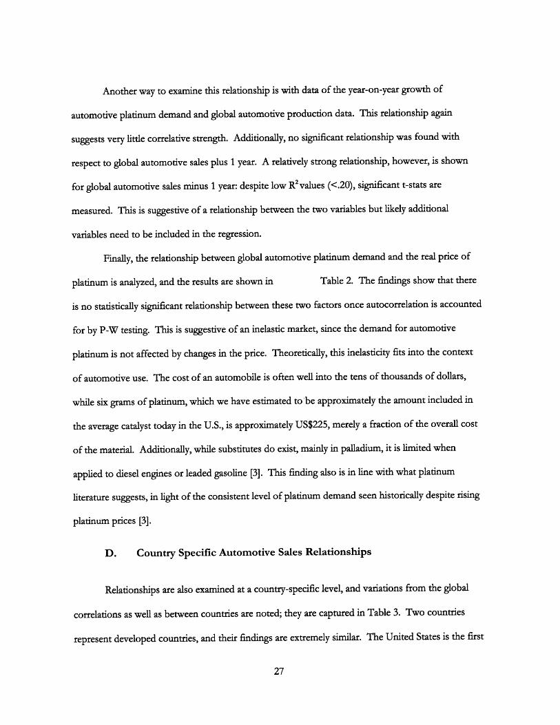
Another way to examine this relationship is with data of the year-on-year growth of
automotive platinum demand and global automotive production data. This relationship again
suggests very little correlative strength. Additionally, no significant relationship was found with
respect to global automotive sales plus 1 year. A relatively strong relationship, however, is shown
for global automotive sales minus 1 year: despite low R2values (<.20), significant t-stats are
measured. This is suggestive of a relationship between the two variables but likely additional
variables need to be included in the regression.
Finally, the relationship between global automotive platinum demand and the real price of
platinum is analyzed, and the results are shown in Table 2. The findings show that there
is no statistically significant relationship between these two factors once autocorrelation is accounted
for by P-W testing. This is suggestive of an inelastic market, since the demand for automotive
platinum is not affected by changes in the price. Theoretically, this inelasticity fits into the context
of automotive use. The cost of an automobile is often well into the tens of thousands of dollars,
while six grams of platinum, which we have estimated to be approximately the amount included in
the average catalyst today in the U.S., is approximately US$225, merely a fraction of the overall cost
of the material. Additionally, while substitutes do exist, mainly in palladium, it is limited when
applied to diesel engines or leaded gasoline [3]. This finding also is in line with what platinum
literature suggests, in light of the consistent level of platinum demand seen historically despite rising
platinum prices [3].
D. Country Specific Automotive Sales Relationships
Relationships are also examined at a country-specific level, and variations from the global
correlations as well as between countries are noted; they are captured in Table 3. Two countries
represent developed countries, and their findings are extremely similar. The United States is the first

of these countries, specifically of interest because of its status as a "first-mover" with regard to the
utilization of catalytic converters for emissions regulation, and thus a significant source of platinum
demand. Japan was on the heels of the U.S. in defining emissions standards, not least because they
knew the requirements established by the U.S. would be enforced on vehicles exported from Japan
to the U.S. [4]. There exist significant similarities in the findings from the two countries. Both U.S.
and Japan findings show that the correlations between automotive sales and any of the
demographics-GDP per capita, population, and total GDP-are not particularly different from
global data results, though both R2 values as well as t-stats are somewhat weaker than those realized
for global data. The only notable difference between the two countries' results comes in the analysis
of total GDP, where Japan shows a significantly higher R2 value than the U.S. along with a slightly
higher t-stat; this difference is, however, relatively small, especially relative to the global findings. As
seen globally, autocorrelation is clearly present but is accounted for by P-W tests, while the
relationships remain statistically significant. Comparison of growth rates for automotive sales and
demographics again show very similar results to the global relationships for each of these developed
nations. As seen before, a strong relation is found between automotive sales growth and GDP per
capita as well as with total GDP; both results are markedly similar to the global data.
The second pair of countries examined are of interest due to their status as developing
countries, specifically as members of BRIC (Brazil, Russia, India, China). From 2005 to 2006, the
last year for which auto sales data was obtained for each country, Brazil car sales grew by over 14%
while India's grew at a staggering 21.6%. These patterns of significant growth, along with a combined
GDP per capita which was less than half that of Japan and less than a third that of the United States
in 2003, suggest that the future market demand will be significant. Understanding how these
markets compare to both global trends as well as trends seen in developing countries is significant
motivation.

The findings for India and Brazil regarding the relation of automotive sales with
demographics present a significant dichotomy: India's data shows extremely strong relationships
between automotive sales and each of the demographics considered, especially in the case of GDP
per capita and Total GDP, whereas Brazil's data shows very weak correlations in the data, with a
maximum R2 value of .20 and a maximum t-stat of only 2.4 after a P-W test. Similarities between
Brazil and India are seen, however, in comparison of the automotive sales growth rate with
demographic growth rates. These results both show relatively insignificant correlations, especially
compared to the global data and developing countries data, albeit India's relationships still tend to be
stronger than Brazil's. Nonetheless, growth of GDP per capita and total GDP, factors for which
statistical significance holds generally constant at the global and developed country level, are
suggested to be only weakly correlated with automotive sales growth, if at all.
E. Country Specific Platinum Demand Relationships
Automotive platinum demand was also examined for both the United States and Japan.
Since platinum demand is a production-driven process (car manufacturers order the platinum for
use in the cars they are producing), developing countries were excluded from this analysis, in part
because the data was not available. Also, these two countries accounted for almost one-third of
total world vehicle production in 2006 [8].
Relationships exhibiting similar strength to that of global data were found for automotive
platinum demand and automotive production. The strengths of these relationships are almost
precisely the same, in terms of statistical significance as measured by R2 values and t-stat values.
Probably due to the countries huge production numbers, this is also similar to the relationship at the
global level.

Price is the last factor considered in defining automotive platinum demand, and the results
for each country are almost as weak as at the global level. These results can be seen in Table 2. This
finding simply reiterates the reasoning stated before regarding the understanding that the automotive
platinum market has historically been considered an inelastic one.
F. Comparison to Palladium Dynamics
Palladium is one of the few substitutes for platinum in its role as a catalyst, albeit in a limited
fashion. As such, examination and comparison of palladium with platinum is of interest, and the
results are captured in Table 4. The findings show that global automotive palladium demand is
related statistically significantly to the demographics GDP per capita, population, and Total GDP,
though these relationships are certainly weaker than in the case of platinum. Again, we might expect
the strongest link to exist between palladium demand and vehicle production, as was seen in the case
of automotive platinum demand. Interestingly, palladium demand does not show a statistically
significant relationship with global automotive production or with U.S. automotive production.
This could be explained by several theories. One is the consideration that palladium was not used
significantly in vehicles until the early 1990s, and thus 15 years of automotive demand captured in
this analysis would be responsible for the use of a relatively small amount of palladium.
Additionally, palladium's role as a substitute with weaknesses in specific areas may imply that price is
a significant factor in a switch away from platinum to palladium. In this vein, palladium prices
spiked in the late 1990s as a response to rapid adoption, and the literature suggests that this would
have made palladium a less attractive substitute for automotive manufacturers [3].
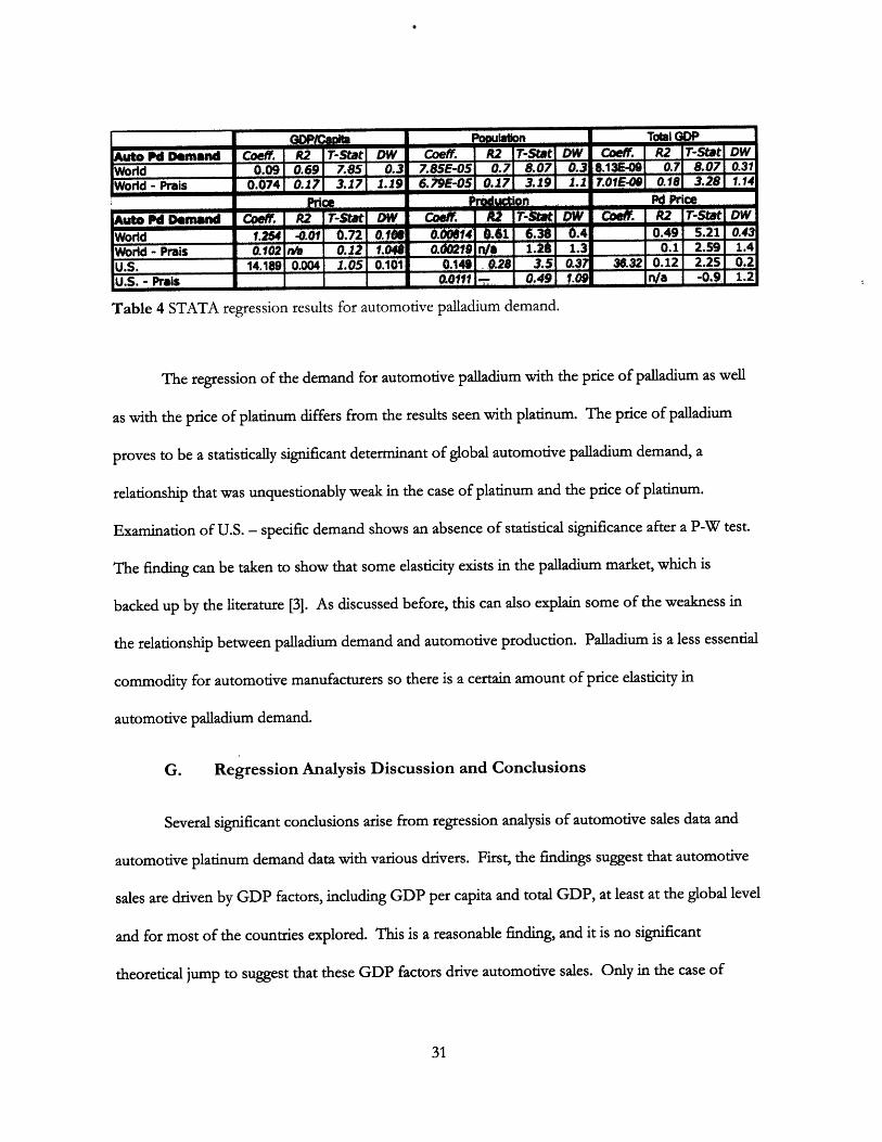
olation Total GDPAuto Pd Demand Coef. R2 T-Stat T-S DW Coeff. R2 ITStat NW Ceff. R2 T-Stat DWWorld 0.09 0.69 7.85 0.3 785E-05 0,7 8.07 0.3 8.13E-09 0. 8.07 0.31
World - Prais 0.0741 0.17 3.17 1.19 6.79E-05 0.17 3.19 1.1 7.oE-0 018 3.281 1.14prie P ,Price
Auto Pd Demand CoeAff. 2 T-Stat OW Coeff T-Stt . 2 T-Stat DW
World 1.254 -0.01 .72 0.1 14 0.49 5.21 63 0.43World - Prais 02 Wa 0.12 1.04 . 1. 1.3 0.1 2.59 1.4
U.S. 14.189 0.004 1.05 0.101 0.14! 0.28 3.51 0.3 3 .32 0.12 2.25 0.2U.S. - Prais 0 . 0111 -- 0.4910 n/a -0. 1.2
Table 4 STATA regression results for automotive palladium demand.
The regression of the demand for automotive palladium with the price of palladium as well
as with the price of platinum differs from the results seen with platinum. The price of palladium
proves to be a statistically significant determinant of global automotive palladium demand, a
relationship that was unquestionably weak in the case of platinum and the price of platinum.
Examination of U.S. - specific demand shows an absence of statistical significance after a P-W test.
The finding can be taken to show that some elasticity exists in the palladium market, which is
backed up by the literature [3]. As discussed before, this can also explain some of the weakness in
the relationship between palladium demand and automotive production. Palladium is a less essential
commodity for automotive manufacturers so there is a certain amount of price elasticity in
automotive palladium demand.
G. Regression Analysis Discussion and Conclusions
Several significant conclusions arise from regression analysis of automotive sales data and
automotive platinum demand data with various drivers. First, the findings suggest that automotive
sales are driven by GDP factors, including GDP per capita and total GDP, at least at the global level
and for most of the countries explored. This is a reasonable finding, and it is no significant
theoretical jump to suggest that these GDP factors drive automotive sales. Only in the case of

Brazil does this relationship lack significant correlation, the reasons for which we are unlikely to
define without a more in depth examination of Brazil's economic factors.
Additionally, we find that automotive platinum demand is correlated significantly with
automotive production at both global and country-specific levels. This relationship is theoretically
the most direct, though there is some expectation that the relationship should be stronger than the
results show. Recognizing that platinum per car is a metric that is also growing over this time may
explain the lack of correlation between platinum demand and automotive production. The findings
also suggest that the market for automotive platinum demand is inelastic, as there is no significant
relationship between automotive platinum demand and price.
Finally, a comparison to palladium shows that platinum has stronger correlations with
demographic factors such as GDP as well as automotive production data. Also, unlike with the
automotive platinum market, the automotive palladium market is price elastic.
These findings serve to characterize the drivers of the automotive platinum market. They
support much of our theoretical understanding of the platinum market while raising additional
questions about the dynamics of this market. Finally, while they do not directly inform the
subsequent platinum market simulation model analysis for the most part, they do allow us to further
inform and understand additional attempts to characterize the automotive platinum market and its
impacts on the overall platinum market.
V. Platinum Market Simulation Model Results
A. Model Structure and Base Case Behavior
Examination of the impact of automotive demand for platinum on the overall platinum
market was achieved through the use of a platinum market simulation model. The platinum market
simulation model's structure is basically captured in Figure 7. Price fluctuations occur in the market
32

as a response to shifts in supply and demand, which in turn can lead to changes in supply and
demand. Price increases on the supply side can increase the incentive for either mining more
material or exploring to define new supplies of that material. Increases in supply can drive the price
down as more material is available to fulfill demand. On the demand side, price increases can cause
those demanding of the material to switch to lower price substitutes or to simply demand less of the
material, decreasing the overall demand. Decreased demand can also drive prices back down as
suppliers attempt to capture more of the market with lower prices. Such are the basic drivers of the
market that must be captured in the model for it to accurately capture the platinum market dynamic.
The automotive sector is no small piece of this puzzle. Automotive platinum demand
accounted for approximately 59% of total primary and estimated secondary platinum demand in
2007 [3]. Additionally, as the results of STATA analysis have shown, the relation between
automotive platinum demand and platinum price has historically been an inelastic one. More recent
news reports on the availability of alternatives for the traditional three-way catalysts and traditional
wash coats indicate that this trend of inelasticity may be breaking. Nanotechnology has been used to
develop new designs for catalytic converters that obtain the same activity with less platinum. Thus
there exists a dichotomy between historical patterns and future expectations [16]. These potentially
shifting market dynamics coupled with significant growth in automotive demand in developing
nations inspire an exploration of the way in which automotive platinum demand impacts the
platinum market as a whole.

Platinum Market
Figure 7: Schematic of the platinum market simulation model [171.
The sheer number of factors that influence even one sector of the platinum market
recommend the use of systems dynamics simulation modeling to capture the complex feedbacks.
The utilization of systems dynamics modeling with applications to the platinum market has been
described previously [1,2]. Both endogenous and exogenous variables are used to capture the
market dynamics. Endogenous variables are those explained by the model and include supply,
demand, and price; exogenous variables are the inputs to the model that inform the endogenous
variables.
An important context to provide is the level of calibration of the model. The model is built
with platinum market data collected from literature. Variables that were not available were estimated
through partial calibration with historical data for primary supply, demand and price normalized by
the producer price index for commodities. The partially calibrated model cannot be used to predict
future trends in endogenous variables. The trends produced by the model that inform analyses are
Supply
Primary Resources- location- ore grade- minera type- extraction
technology
Secondary Resourcesproduct type
- recyclingefficiency
Rate of Consumption
I
DemaPRICE
Products- produc- growth- price e- substittechno
Rate of Disposal
nd
t demand
lasticityutionlogy
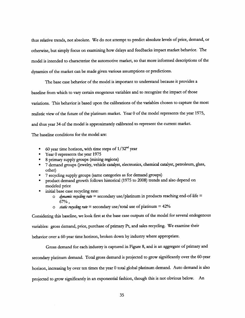
thus relative trends, not absolute. We do not attempt to predict absolute levels of price, demand, or
otherwise, but simply focus on examining how delays and feedbacks impact market behavior. The
model is intended to characterize the automotive market, so that more informed descriptions of the
dynamics of the market can be made given various assumptions or predictions.
The base case behavior of the model is important to understand because it provides a
baseline from which to vary certain exogenous variables and to recognize the impact of those
variations. This behavior is based upon the calibrations of the variables chosen to capture the most
realistic view of the future of the platinum market. Year 0 of the model represents the year 1975,
and thus year 34 of the model is approximately calibrated to represent the current market.
The baseline conditions for the model are:
* 60 year time horizon, with time steps of 1/ 3 2nd year* Year 0 represents the year 1975* 8 primary supply groups (mining regions)* 7 demand groups (jewelry, vehicle catalyst, electronics, chemical catalyst, petroleum, glass,
other)* 7 recycling supply groups (same categories as for demand groups)* product demand growth follows historical (1975 to 2008) trends and also depend on
modeled price* initial base case recycling rate:
o dynamic reyclng rate = secondary use/platinum in products reaching end-of-life =67%,
o static regycing rate = secondary use/total use of platinum = 42%
Considering this baseline, we look first at the base case outputs of the model for several endogenous
variables: gross demand, price, purchase of primary Pt, and sales recycling. We examine their
behavior over a 60-year time horizon, broken down by industry where appropriate.
Gross demand for each industry is captured in Figure 8, and is an aggregate of primary and
secondary platinum demand. Total gross demand is projected to grow significantly over the 60-year
horizon, increasing by over ten times the year 0 total global platinum demand. Auto demand is also
projected to grow significantly in an exponential fashion, though this is not obvious below. An

interesting observation is that jewelry demand grows typically in response to price drops, and clearly
decreases over the last 20 years of the model, which corresponds with the price outputs seen in
Figure 12.
2E*09
1 8E+09
1 6E*09
1 4E39
1 2E*09
S1E09
8OOOOO
600000W
40000000
20000000
0
10 15 20 25 30 35 40 45 50 55 60
Y"n
Other
* Glass~
a Petroleum
8 Chemical
4 Electronics
SAutomotrve
a lewelry
Figure 8 Gross platinum demand, stacked by industry, over 60-year time horizon
Trends in recycled platinum versus primary platinum are also of interest. These two outputs
are captured in aggregate in Figure 9 and Figure 10, respectively. With specific regard to automotive
primary and secondary platinum demand, Figure 11 shows that the percentage of primary and
recycled platinum utilized is projected in the base case to remain relatively constant throughout the
60-year time frame. This consistency provides an interesting baseline, as we examine whether
variations in exogenous variables may affect this trend.

9 00t*02
8.00o02 4
7 00E 02
6 .00*02
4.00E02
3006E*02
100E+02 1
O.OO0000
Time (.5 yea)
Figure 9 Sales recycling by industry, base case, 60 year horizon.
1.20E+09
1.00E+09
i--6.00+08 T4.00.406
2.00E08
O.0E*00
1 6 11 16 21 26 31 36 41 46 51 56 61 66 71 76 91 86 91 96 101 106 111 116 121
Tim (.5 years)
Figure 10 Primary purchase of platinum by industry, base case, 60 year horizon.
SOther
SGlass
* Petroleum
* Chemical
* Electroncs
a Jewlry
SOther" Glass
* Petroleum
* Chemical
* lectronlcs
SWtry

7000%
U
E
S5o.00%
30.00%
10. 00%-N
OA M - ---------
0.00 10.00 20.00 30.00 40.00 50s00 60.00 70.00
Trhw (wrsn)
Figure 11 Automotive industry primary versus recycled platinum use by percentage, base case, 60
year horizon.
Another output examined in the base case is price. Price variations captured in Figure 12
suggest that price will more than double, in real terms over the 60-year time horizon. This price
trend is likely explained by the fact that the quality of ore over time will likely degrade, thus
increasing the cost of extraction and thus the overall price. The increase is certainly not a linear one,
as price looks to increase rapidly for a period of time, then drop relatively sharply and return slowly
to levels near those that were seen before an increase. This may be accounted for by the lag in
bringing supplies online in response to increases in demand. These demand increases may push
price upwards as less cost-effective supplies are utilized to meet this demand, followed by a
significant drop and tapering-off of the price once these supplies are able to meet demand once
again. The price tapers downward in the period following this peak, thus reducing the incentive for
suppliers to increase or even maintain supplies, especially less cost-effective ones. Eventually,
demand increases again, or supply falls to an insufficient level, and the price peak occurs once again.

This is a pattern of interest because price variations create an inherently more volatile environment
for price-taking end users.
70
60
40
0 10 20 30 40
Figure 12 Price of platinum over 60-year time horizon.
B. Exogenous Variable Sensitivity Analysis
50 60
We utilize sensitivity analysis to answer the question of how various scenarios in the
automotive market may affect the platinum market as a whole over our time horizon. Numerous
scenarios and possibilities exist for the future of the market, but our focus on the potential for
growth in developing economies informs some of these analyses, as does the potential for increased
substitution options for platinum use that may lead to increased elasticity.
A high level review of the theoretical impact of high automotive platinum demand growth
rates will help inform our results. High automotive platinum demand growth rates will dearly
increase demand dramatically and thus can drive up the price of platinum if new supply does not

come on line immediately. This new supply would likely come on line relatively slowly, as there is a
significant monetary and time investment to set up new mines; new mines are also likely to be of a
lower ore quality than those utilized currently, further exasperating the delay on the supply side,
since a greater quantity of ore must be extracted to achieve the same yield of platinum realized with
higher quality ores. These delays will thus drive an increase in price, or at least prevent price from
falling until supply is increased. In response to this increased price, substitute materials become
more viable, especially if they are of lower cost. This substitution in turn decreases demand and thus
feeds back to lower prices. As explored, however, this is not the trend seen historically in the
market for automotive platinum demand, which is shown to be inelastic. As such, this mechanism
for "relieving" a particularly high level of price via substitution has not been seen in the automotive
platinum demand market, leading to significant price increases over time.
With this theory and behavior in mind, the impact of both various levels of growth in
demand as well as various levels of elasticity are inquiries of interest. Again, these are informed by
more than simply high level market dynamics, but by real-time considerations of factors that may
influence the market: the evident automotive market potential in developing countries which is
inextricably tied to platinum demand potential, and the increased availability of potential substitutes
for platinum in TWCs. These analyses are described in Table 5. In summary, to examine the
simultaneous effects of various exogenous automotive platinum demand growth rates and various
levels of automotive platinum demand elasticity, growth rates were varied at three distinct levels of
elasticity, labeled as low, medium, and high and corresponding to values of .05, .30, and 1.0,
respectively. The endogenous outputs considered in each scenario were total platinum gross
demand, automotive platinum gross demand, and price of platinum.

Scenario Exogenous Assigned Exogenous SensitivityVariable #1 Value Variable #2 Range
Base case elasticity, vary Demand 0.05 Demand -0.01 to 0.10growth Elasticity Growth
Medium elasticity, vary Demand 0.30 Demand -0.01 to 0.10growth Elasticity Growth
High elasticity, vary Demand 1.0 Demand -0.01 to 0.10growth Elasticity Growth
Table 5 Analysis scenarios examining demand elasticity and demand growth.
1. Low Elasticity
The first scenario to consider is that which utilizes the base case demand elasticity, which, at
a value of only 0.05, is also the scenario considering low elasticity. As shown through STATA
analysis, this level of elasticity (close to 0) is representative of historical market relationships. The
first endogenous variable whose output we will examine within the base case scenario is automotive
platinum gross demand. The first finding, the average platinum gross demand, is shown in Figure
13. The average platinum gross demand scales with growth rate exponentially. The escalation of
gross demand caused by increases in the growth rate is much more significant than the increases in
total platinum gross demand, shown later in Figure 14. Theoretically this is reasonable, as it is the
automotive demand growth rate we are varying, so the impact on the automotive sector should be
relatively greater than the impact on the total platinum demand market. Indeed, the average
automotive gross demand at a growth rate of 10% is over 17 times that of the gross demand given a
growth rate of -.1%, whereas the difference in the total gross demand from the previous output was
less than a multiple of 2. The exponential relationship is important to note as well. If we consider
the significant recent growth rates for developing countries, such as 14% for Brazil and 21% for
India, even considering that these rates are only a portion of the overall automotive platinum
demand markets, any consistency in these rates year after year could lead to momentous, non-linear

increases in overall gross demand. A more interesting aspect of the difference between the total
platinum gross demand and automotive platinum gross demand is that the automotive industry is
one that has historically had very low elasticity, but some of the other industries have higher
elasticity, such as the jewelry industry. While demand for platinum in TWC's can drive up platinum
price during periods of growth of the automotive industry, jewelry demand will drop, partially
offsetting the increased platinum demand in automotive.
400000
3500000X)
25000000
-0.02 0 0.02 0.04 006 0.08 0.1 0.12
Automorde PItmnm Growth Rate
Figure 13 Automotive sector gross platinum demand, base case elasticity, varying growth.
Figure 14 captures the pattern of the average total platinum gross demand. The results show
that increases in the automotive growth rate causes an increase in total gross demand, which is a
reasonable relationship. Interestingly, the slope of this relationship increases as demand growth
approaches 10%. This is important because it shows that increases in growth rate impact the total
gross demand for platinum in a significant, non-linear fashion.

0
'50000oW
0.02 0.04 0.06 0.08 0.1 0.12-0.02
AutomaeW IPbtbwm Growth RMt
0 0.02 0.04 0.06 008
AkVIORWW Pbdwnr eomd Growth RAW
09'
0.8
o s0.7
01
0.65
0-6
* StDev
lStDev (Normalted)
0.1
Figure 14 Total platinum gross demand average and standard deviationsbase case elasticity, varying growth.
Ia.
700 T
-0.02
(regular and normalized),
ssoDooo f

As demand growth increases, so too do both the regular and normalized standard deviations.
The implications of these findings are distinct, however, from those realized from the averages. The
increase in standard deviation suggests that increases in demand growth cause the volatility of total
gross demand to increase. Theoretically, this is explained first by the fact that higher growth rates
can lead to higher prices, and second because higher prices in elastic markets can lead to substitution
and thus decreases in demand, while lower prices (which may come as a result of this decrease) can
push demand higher once again. By the mechanism described here, higher growth rates will, over
the 60-year horizon, cause these fluctuations to occur more frequently and be of higher magnitude
than the case of low growth rates. Finally, one aspect of the results is important with regard to both
average total gross demand as well as the standard deviation: that changes in an automotive-specific
variable have a noticeable impact on the platinum market as a whole.
The final endogenous variable examined is platinum price, and the results are captured in
Figure 15. The general trend is that price increases as automotive platinum demand growth
increases, which suggests two impacts. The first is that the mechanism described at the beginning of
this section, which suggests that, in a relatively inelastic market, increased growth causes a disparity
between supply and demand which leads to increased prices, is essentially reasonable. The second is
that changes in automotive-specific growth rates indeed have a noticeable impact on the overall
market, as seen with total gross demand. The general trend is an increasing slope between price and
demand growth as growth increases, suggesting that this relationship is non-linear, similar to the
behavior seen in previous outputs. The magnitude of the impact is also significant: the price at 10%
growth is approximately double that seen at rates around 0%. A shift of this magnitude certainly
implies that a general trend of increased demand growth may have a significant impact on price,
suggesting that substitution or increase elasticity in the market could arise as a result.

0.04 0.06
Autvomote Platinum Demand Growth
0
0 0.02 0.04 0.06 0,08 0.1 012
Demand Growth of AuomoWUe
Figure 15 Platinum price, average and standardcase elasticity, varying growth.
deviation (regular and normalized), base
80
70
30 ---
-0.02 0.02
40
0.06 0.12
U
30 -
20
0.9
0.8
0.07
0.6
0.4
tL
0.3
02
* StDev -Reg
*StOev- Norm
0 +
-0.02
0.1
..... ---.

The behavior of the regular and normalized standard deviations are very similar in the case
of platinum price. Both suggest an overall increase in the standard deviation as automotive demand
growth increases, in an exponential fashion; however, the average price trend suggests asymptotic
behavior, which is not seen in the standard deviation trend. Since the dynamics of price are such
that it will initially increase as a response to growth in demand due to the shortcomings of supply in
meeting demand, and then will subsequently fall as more supply comes online to meet this demand
increase, the greater the growth that drives this mechanism, the more volatility experienced in the
market. The onset of the increased volatility occurs at lower growth rates than the onset of the onset
of the sudden increase in the average price. Additionally, the fact that the growth driver of this
relationship, as has been seen in relationships with other endogenous variables, is exponential
suggests that even slight increases in growth can have a significant impact on price. Understanding
the base case for price is perhaps the most important of any of the endogenous variables assessed, as
it arguably acts as the market's output, integrating the shifts in all the other aspects of the market.
Also, it is the most directly applicable to the end user of platinum, and perhaps the simplest way to
show or explain the impacts that a change such as significant increases in automotive industry
demand growth rates could have on the bottom line.
2. Medium and High Elasticity
Having established a foundation for further analysis, we can now examine the effects of
various values of automotive platinum demand elasticity on the endogenous variables. As before,
the first endogenous variable of interest is automotive platinum gross demand, and the outputs are
viewed by their averages and standard deviations (in this case only normalized standard deviations

are presented). For automotive platinum gross demand, results are captured in Figure 16 and Figure
17.
The trends for average automotive platinum demand are fundamentally similar in that they
are non-linear, exponential relationships. Variation occurs in how steep the slope escalates over the
given range of automotive platinum demand growth rates. This escalation clearly occurs most
quickly relative to the increase in growth rates at low elasticity, and suggests it may even have
asymptotic behavior, which could be seen given only a few more percentage points of growth. As
elasticity rises from low to medium, and from medium to high, the escalation of the slope
diminishes; the exponential relationship between growth rate and gross platinum demand for low
elasticity at 10% growth is an extremely shallow slope that looks to be surpassed by the slope of the
low elasticity case at a growth rate of .4% or less. Theoretically, higher platinum demand growth
rates will drive increased gross demand, which will also increase price. At low elasticity, however,
there is very low sensitivity to price, and thus demand will grow without the consequences of
increased price discouraging that growth. As the elasticity increases, the increase in price resulting
from increased demand will discourage further growth from occurring.
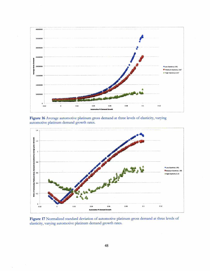
Ltw Eo U"cW (.05)
SMedum n lsdty 1.30)"
A "tigh ElastkAy (1.01
0 0.02 0,04 0.06 0.08 0.1
Aumltdwe Pt ft mm mgh
Figure 16 Average automotive platinum gross demand at three levelsautomotive platinum demand growth rates.
12I04
01II"j 0
of elasticity, varying
*Lw Elanty OS.05)
A di ElastitWy (1.0)
0.12
at three levels of
0 0.02 0.4 0.06 0.08 0.1
Aumtowe Pt Demnv mGrth
Figure 17 Normalized standard deviation of automotive platinum gross demandelasticity, varying automotive platinum demand growth rates.
50000 ,
J -,IWOW!1W060t1 tl000+
---1-

The normalized standard deviation results present close similarities between the volatility of
low and medium automotive platinum gross demand. These relationships are essentially the same,
except that the medium elasticity is shifted up approximately 0.05%, suggesting that it takes a
marginally higher growth rate to capture the same trend between growth rate and standard deviation
of gross demand for low and medium elasticities. The results for high elasticity are not as drastically
different as initial observation may suggest, as they loosely follow the same general trend as the
others. In each case, the pattern suggests that there is some minimum standard deviation at a given
growth rate, which is very close to 0% in the high elasticity case and increases for the other results.
Lack of volatility in a market may suggest a balance between supply and demand, and thus this
minimum represents the growth rate for which the market is relatively stable. Considering the case
of low elasticity, demand will be affected only minimally by shifts in price, and thus any growth rate
at all will increase demand and disrupt market equilibrium. In the cases of the higher elasticities, the
results suggest a "buffer," provided by the higher rates of elasticity; this buffer allows the market to
absorb growth rates of a particular level due to this increased price sensitivity, which will ultimately
offset some of the demand growth.
For growth rates greater than this minimum, the relationship between growth rates and
standard deviation of gross demand is close to linear, although the slope does become shallower in
each case as growth rates near 10% are seen. This supports the basic theory that has been presented
for increases in volatility caused by increasing growth rates, whereby these growth rates drive up
demand, which drives up prices, which can drive demand downward yet again, creating significant
fluctuations in demand.
Total platinum gross demand is the next endogenous variable of interest and results for this
are captured in Figure 18 and Figure 19. The general trends for the average total platinum gross
demand are similar to those of automotive platinum gross demand. The exponential relationships

for each show less slope escalation in the given growth rate range as elasticity increases. Again, this
is due to the offset of demand increases that comes of higher elasticity and thus price sensitivity,
causing demand only to grow marginally relative to growth rate in the case of high elasticity.
Interestingly, the data for low and medium elasticities diverge at a growth rate of approximately 8%,
suggesting that the impact of automotive platinum demand growth rates is much more noticeable
after this level of growth is achieved, a finding reinforced by the standard deviation data.
....... . . .. .. . .. ..t ~ ~~ ~~ ....... .. .. ... ... ... ..-- .. .. .. .. ... ....-- ... ..-------
I -int
wM
WWWW
ft+LOW Mladt (.OS)
Mdkun mUnart o.30
A Hh tWnaty (LO)
£
b4~
5OOO OO--,0.O2 o 0.02 0.04 0.0
A0mou e Pt Onmind Grwm
00S 0.1
Figure 18 Average total platinum demand at three levels of elasticity, varying automotive platinumdemand growth rates.
0.12
-, - - - --- - -- - --

0.9
4 1M6i1h EIastity (1.0)
0. 06
0 0 002 0 00 0.04 006 008 01 0.12
Automogt Pt Omand Growth
Figure 19 Normalized standard deviation of total platinum demand at three levels of elasticity,varying automotive platinum demand growth rates.
Normalized standard deviation results suggest that until an automotive platinum demand
growth rate of approximately 8% is reached, the volatility at each elasticity level is similar. This
suggests that a growth rate of 8% or higher must be attained for the automotive platinum sector's
growth rate to impact the volatility of the platinum market as a whole. Indeed, after 8%, volatility in
relation to growth rate increases significantly for low elasticity, noticeably for medium elasticity, and
relatively insignificantly for high elasticity. Again, the price sensitivity that comes with an
assumption of low elasticity is relatively low, causing demand to be pushed up in response to high
growth rates. In this case, it takes a growth rate of over 8% to achieve this.
The last endogenous variable of interest is platinum price. The results are presented in
Figure 20, Figure 21, and Figure 22. The average platinum price results show increasing price over
time with increasing automotive platinum demand growth rates. The theory discussed at several
points applies here as well, as higher growth rates drive up demand, which in turn cause price to rise
51

since additional supply cannot come online as quickly as demand grows. The elasticities play a role
and clearly show distinguishing patterns for average price; this stems from the fact that low elasticity
markets will not realize a decrease in demand given a price increase, thus demand will continue to
grow despite this increase in price. The results also suggest a divergence point at an automotive
platinum demand growth rate of approximately 6%, after which the average platinum price follows
noticeably different increases as growth rates increase for each elasticity scenario. Low elasticity
prices grow very rapidly after 6% growth, increasing approximately 30% to the price at 10% growth
(extreme outliers put this price increase in the range of 500% or more, but we consider the visible
graph as a reasonable bound to avoid outliers). High elasticity prices grow very little after the 6%
mark, with growth of only about 5%. Medium elasticity prices grow at a level between these two
extremes, of approximately 20%.
-0.02 0 002 004 0.06 O08 0.1 0.12
Asmate Pt Demad emmt
Figure 20 Average platinum price at three levels of elasticity, varying automotive platinum demand
growth rates. Outliers excluded from analysis include a peak price of 334.9 for the low elasticityscenario.

O.9'
.5 *0ow5a~slatY.05Io6
6. i-- -- ----- -- ----
01
0'-0.02 0 002 0-04 0.06 008 01 0.12
AutoafOe Pt Demand Growth
Figure 21 Normalized standard deviation of platinum price at three levels of elasticity, varyingautomotive platinum demand growth rates.
The standard deviation results show the same pattern of divergence at an automotive
platinum demand growth rate of around 6%. In this case, the impact of the various elasticities is
even more extreme: for low elasticity, the price grows by approximately 100%, even neglecting
outliers; for medium elasticity, this growth is also substantial, around 75%; and for low elasticity, the
growth is minimal, at 10% or less. The impact of various levels of automotive platinum demand
elasticity on the standard deviation of price, and thus the volatility of price, occurs because increased
demand growth of course drives demand to increase. Since supply cannot meet this new level of
demand immediately, price increases and represents relative scarcity of the material. In a high
elasticity market, the price will drive purchasers to use substitutes or generally demand less of the
material, causing price to shift back down before reaching a significant level. Thus, since the price
does not need to reach the same level to drive this drop in demand as it would need to reach for the
same substitutions to occur in a lower elasticity market, the overall volatility of the market is low
53

relative to the lower elasticity market. In the low elasticity market, demand is less prone to drop
given equivalent price increases and thus price will rise much higher, causing a higher standard
deviation overall.
The trend of platinum price over time for each of these scenarios is also of interest and is
captured in Figure 22. High elasticity, as seen previously with the average platinum price, is
consistently the lowest price scenario. After the first peak and trough of the fluctuations in price,
the price clearly varies much less than in the case of low or medium elasticity. Ultimately, the
highest price reached is significantly lower than in either of the other two scenarios.
The platinum price trends for medium and low elasticity are very similar. The most
noticeable difference is that low elasticity tends to be slightly delayed relative to medium elasticity.
This is reasonable, since low elasticity markets should have a slightly lower propensity to substitute
as a reaction to high prices, an action that drives the demand down and thus the price as well. Even
though the prices drop significantly after the peak for each scenario, the drop for the low elasticity
case should occur slightly later than for medium elasticity, and that is suggested by the results.
Extrapolating this reasoning may suggest that high elasticity should thus have an even smaller delay
relative to medium elasticity, which does not look to be the case. The reasoning here could be that
the market is as a whole more stable when there is high elasticity, since demand increases which
cause price to rise significantly are eased by the markets propensity to look for substitutes. Thus
price increases are less abrupt, causing price to peak later relative to the lower elasticity scenarios.
This would offset the relatively smaller expected delay on the downside of the price peak by
increasing the delay seen on the upside.

80
70
-Low Elasdtlty (.05)
5so Ihigh Elistoty (1.01
Medium Elastity (.30)
40
30
0 10 20 30 40 50 60 70
rTme (VeS)
Figure 22 Platinum price over time at three levels of elasticity, 60 year time horizon.
C. Platinum Market Simulation Model ConclusionsExploration of the base case results for various endogenous variables of the platinum market
simulation model, as well as the effects of various sensitivity analyses, has allowed the automotive
platinum market to be further characterized both as an isolated entity and with regard to its impact
on the overall platinum market. The base case relationships provide important insight into the
overall trends seen by the model. Over a 60-year time horizon, significant growth in both total
platinum gross demand and automotive platinum gross demand is expected, and these trends are
expected to be exponential. Price is expected to rise over the time horizon as lower grades of ore
are utilized to fulfill primary platinum demand. Additionally, price is expected to fluctuate over this
time period, due to the lag of bringing supply on line to meet rising platinum demand requirements,
suggesting a volatile environment for price-taking end users. Such price fluctuations are not new for
the platinum market.
Sensitivity analyses of the base case conditions allow us to isolate the effect of automotive
platinum demand growth on various endogenous variables. The effects on automotive platinum

gross demand show that average gross demand over the time horizon grows exponentially with
automotive industry growth rates as a result of low price elasticity. Additionally, the standard
deviation of automotive platinum gross demand increases with increasing growth rates, as supply has
a difficult time meeting the jumps in demand associated with these growth rate increases, causing
price fluctuations which in turn create demand fluctuations. The findings for total platinum gross
demand suggest that it follows similar overall trends as automotive platinum gross demand, though
smaller relative impacts are seen because as prices increase industries with high price elasticity, such
as the jewelry industry, will decrease their use of platinum and offset the automotive industry
platinum demand growth. One key takeaway of this analysis is that variations in automotive
platinum sector-specific growth rates can noticeably impact the overall platinum market.
The relationship between automotive platinum demand growth rates and price is also
established. The modeling results indicate that very high growth rates in the automotive industry
could push prices high if automotive manufacturers continue to behave as if platinum prices do not
matter (i.e. exhibit low price elasticity). This is an important indicator of automotive platinum
demand growth impacts, as price is the clearest signal to the end-user of platinum.
The findings clearly show that automotive demand growth has a significant effect on a
variety of important variables in both the automotive platinum market as well as the platinum
market as a whole, noticeably affecting factors such as total gross platinum demand and platinum
price. These results are significant due to the potential for momentous growth in automotive sales
in developing countries. Regression analysis has shown that automotive sales, which inherently
drive automotive production, are a driver for automotive platinum demand at a global level as well
as for specific countries.
Comparison of these sensitivity relationships at various levels of elasticity allows us to isolate
the effect of automotive platinum demand elasticity on various market variables. Lower demand

elasticity causes gross platinum demand to increase more significantly at a given level of automotive
demand growth. This is driven by the lower propensity for substitution in a lower elasticity market.
Lower elasticity values, which represent a lower degree of substitution, also increase the volatility of
gross demand, since this causes price to increase significantly more than in the case of high elasticity.
Additionally, at and below a set growth rate, the market's elasticity and propensity to substitute for
the lower price material allow growth in automotive demand without significant increases in price
volatility. The automotive industry growth rate at which there is a significant onset of price volatility
occurs is higher for higher levels of elasticity in the automotive industry.
Elasticity also impacts the trend of price over time. Low elasticity markets are delayed
relative to higher elasticity markets due in part to their lower propensity to seek substitutes. This
causes a delay in reaction to high prices, leading to higher average prices than in the case of higher
elasticity. Notably, this delay occurs on both the upside and downside of price peaks, which works
to create less abrupt price increases and decreases for high elasticity markets.
Two chief findings define the impact of growth on automotive platinum demand: first,
minimums in volatility associated with specific growth rates are shown to exist, and suggest that
there is a "buffer" in the market given higher levels of elasticity which can account for some level of
demand growth; second, the impacts of automotive platinum demand growth on the overall
platinum market look to occur only beyond a minimum level of demand growth, somewhere in the
range of 6-8%. These two findings are likely linked, as both address the ability of the market to
accommodate demand growth to some level but not beyond that.
The implications of these findings are important since the level of elasticity governs market
behavior beyond these milestone growth rates. Although the automotive platinum market has
historically been an inelastic market, we have discussed several events that may suggest an increase in
elasticity. If this is the case, the behavior of both the automotive platinum demand market as well as

the overall platinum market will undoubtedly be influenced significantly. Understanding this
potential is important for any player in the market, as this shift in market dynamics could make
historical market patterns obsolete.
VI. Future WorkBoth regression analysis and use of the platinum market simulation model have allowed us
to characterize the automotive platinum market, including its impacts on the overall platinum
market. Future work in this area has a variety of potential starting points. One of these is an
analysis of the dynamic between primary and secondary platinum demand in the automotive market.
Obtaining platinum from discarded vehicles is form of recycling that may ease the impact of
potential automotive platinum demand growth on primary platinum suppliers. Further study of
recently developed technologies that aim to reduce the required amount of platinum in catalysts is
also in order, an understanding that could be used to develop a more current view of the automotive
platinum market.
VII. Bibliography
1. Alonso, E., et al., MaterialAvailabily and the Supply Chain: Risks, Effects, and Responses.Environmental Science & Technology, 2007. 41(19): p. 6649-6656.
2. Alonso, E., F.R. Field, and R.E. Kirchain, A Case Study of the Availabily of Platinum GroupMetals for Electronics Manufacturers, in International Symposium on Electronics and the Environment2008, IEEE: San Francisco.
3. CPM Group, Platinum Group Metals Yearbook. Vol. 22. 2007, Hoboken, NJ: John Wiley &Sons. 219p.
4. Gerard, D., Lave, L.B. Implementing technology-forcing policies: The 1970 Clean Air ActAmendments and the introduction of advanced emission control systems in the UnitedStates, Technol. Forecast. Soc. Change 72 (2005) (7), pp. 761-778.
5. Heck, R. and R. Farrauto, Automobile exhaust catalysts. Applied Catalysis A, General, 2001.221(1-2): p. 443-457.
6. Shelef, M. and R. McCabe, Twenty-fveyears after introduction of automotive catalysts: what next?
Catalysis today, 2000. 62(1): p. 35-50.7. Kitco Inc. Charts and Data. April 2008; Available from: http://www.kitco.com/charts/.8. Ward's Communications Inc., Ward's world motor vehicle data. 2007, Ward's Communications:
Southfield, MI. p. v.9. Davis, S. and S. Diegel, Transportation energy data book. Washington, DC, 2006.10. "China auto sales surpass US for 3" month." Yahoo! Finance. (8 April 2009). 23 April
2009.11. Hamilton, L.C. "Statistics with STATA." Canada: Brooks/Cole, 2004.12. Johnson Matthey Precious Metals Marketing. Platinum Today. March 2008; The world's
leading authority on platinum group metals. Available from:http://www.platinum.matthey.com/.
13. U.S.G.S. Minerals information. April 2009; Available from: Data gathered from MineralYearbook and Mineral Commodity Summary found online athttp://minerals.usgs.gov/minerals/.
14. Heston, A., Summers, R. and Aten, B., Penn World Table Version 6.2, Center forInternational Comparisons of Production, Income and Prices at the University ofPennsylvania, September 2006.
15. Bureau of Labor Statistics. Producer Price Indexes. May 30, 2008; Available from:http://data.bls.gov/cgi-bin/surveymostwp.
16. "Mazda develops catalyst material structure using nanotechnology." DieselNet. (5 October2007). 25 April 2009.