an exploration of adolescent obesity determinants

University of South FloridaScholar Commons

Graduate Theses and Dissertations Graduate School

5-13-2016

An Exploration of Adolescent ObesityDeterminantsAnastasia King SmithUniversity of South Florida, [email protected]

Follow this and additional works at: http://scholarcommons.usf.edu/etd

Part of the Economics Commons

This Thesis is brought to you for free and open access by the Graduate School at Scholar Commons. It has been accepted for inclusion in GraduateTheses and Dissertations by an authorized administrator of Scholar Commons. For more information, please contact [email protected].

Scholar Commons CitationSmith, Anastasia King, "An Exploration of Adolescent Obesity Determinants" (2016). Graduate Theses and Dissertations.http://scholarcommons.usf.edu/etd/6394

http://scholarcommons.usf.edu/?utm_source=scholarcommons.usf.edu%2Fetd%2F6394&utm_medium=PDF&utm_campaign=PDFCoverPages

http://scholarcommons.usf.edu/?utm_source=scholarcommons.usf.edu%2Fetd%2F6394&utm_medium=PDF&utm_campaign=PDFCoverPages

http://scholarcommons.usf.edu?utm_source=scholarcommons.usf.edu%2Fetd%2F6394&utm_medium=PDF&utm_campaign=PDFCoverPages

http://scholarcommons.usf.edu/etd?utm_source=scholarcommons.usf.edu%2Fetd%2F6394&utm_medium=PDF&utm_campaign=PDFCoverPages

http://scholarcommons.usf.edu/grad?utm_source=scholarcommons.usf.edu%2Fetd%2F6394&utm_medium=PDF&utm_campaign=PDFCoverPages

http://scholarcommons.usf.edu/etd?utm_source=scholarcommons.usf.edu%2Fetd%2F6394&utm_medium=PDF&utm_campaign=PDFCoverPages

http://network.bepress.com/hgg/discipline/340?utm_source=scholarcommons.usf.edu%2Fetd%2F6394&utm_medium=PDF&utm_campaign=PDFCoverPages

mailto:[email protected]

An Exploration of Adolescent Obesity Determinants

by

Anastasia King Smith

A dissertation submitted in partial fulfillment

of the requirements for the degree of

Doctor of Philosophy

Department of Economics

College of Arts and Sciences

University of South Florida

Co-Major Professor: Gabriel A. Picone, Ph.D.

Co-Major Professor: Philip K. Porter, Ph.D.

Murat Munkin, Ph.D.

Richard Smith, Ph.D.

Date of Approval:

April 29, 2016

Keywords: obesity, principal component analysis, school wellness policy

Copyright © 2016, Anastasia King Smith

Dedication

To Warren for his constant support, enduring love and baking chocolate chip cookies

just when I needed them.

I would not have gotten through this doctorate if it wasn’t for him.

Acknowledgments

As with any journey in life, there are many people who help in countless ways along the

path. In particular, I would like to thank the members of my dissertation committee; Dr. Gabriel

Picone, Dr. Phillip Porter, Dr. Murat Munkin, and Dr. Richard Smith, for their time in serving on

my committee, reviewing my research, and providing their expert advice. In addition, I am very

grateful to Dr. Andrei Barbos for his assistance and guidance through this last stage of the

dissertation at a time when I was questioning my own ability to finish.

I would also like to thank my dear friend, Dr. Natallia Gray. You are a source of strength,

love, and care to everyone around you and I am most grateful to be a part of that circle. I will

forever hold dear fond memories of late night office chats, Starbuck’s library runs and sharing all

of the wonderful moments in our lives that resulted from the universe throwing us together at the

same time in graduate school.

Also, a special thank you to Dr. Brad Frazier, colleague and friend at Pfeiffer University;

while working on the dissertation at a distance from my committee and being at an unproductive

place for quite some time, the timely resources you provided came with perfect timing! I would

also like to thank the Department of Economics for supporting my studies at USF. A special

thank you to staff assistant Diana Reese, who regardless of answering the same questions for

many students over the years, always had a smile and was so very helpful in every way possible.

For those who have been a part of my academic journey these past several years, I would like to

express my sincere gratitude for every moment of encouragement that you provided.

i

Table of Contents

List of Tables ................................................................................................................................ iii

List of Figures .................................................................................................................................v

Abstract ......................................................................................................................................... vi

Chapter 1: Introduction ....................................................................................................................1

Chapter 2: Background of Adolescent Obesity ...............................................................................4

2.1 Physical and Social Impact of Adolescent Obesity .....................................................11

2.2 Economic Costs of Adolescent Obesity ......................................................................12

Chapter 3: Background of the Child Nutrition and WIC Reauthorization Act of 2004 ................14

Chapter 4: Literature Review .........................................................................................................18

4.1 Obesity and Rational Choice Theory ...........................................................................18

4.2 Obesity and Behavioral Economics .............................................................................21

4.2.1 The Case for Paternalism ..............................................................................21

4.3 Adolescent Obesity and Public Policy Intervention ....................................................22

Chapter 5: Conceptual Framework ...............................................................................................25

Chapter 6: Research Methodology ................................................................................................28

6.1 Model Specification .....................................................................................................28

6.2 Dependent Variable .....................................................................................................28

6.3 The Primary Explanatory Variable ..............................................................................31

6.4 Other Explanatory Variables........................................................................................31

Chapter 7: Data Sources ................................................................................................................34

7.1 Youth Risk Behavior Surveillance Survey ..................................................................34

7.2 The School Health Policies and Practices Study .........................................................35

7.2.1 Principal Component Analysis .....................................................................37

7.2.2 Polychoric Principal Component Analysis Implementation .........................39

7.2.3 Constructing the Wellness Policy Indices.....................................................44

7.3 Other Data ...................................................................................................................46

Chapter 8: Descriptive Statistics ....................................................................................................49

8.1 Adolescent BMI ..........................................................................................................49

8.2 Explanatory Variables .................................................................................................52

ii

Chapter 9: Empirical Implementation ............................................................................................55

9.1 OLS Estimation ............................................................................................................55

9.1.1 Determinants of Individual Adolescent BMI Regression .............................55

9.1.2 Regression Post Wellness Policy Implementation Year ...............................56

Chapter 10: Results ....................................................................................................................57

10.1 OLS Results ...............................................................................................................57

10.1.1 Determinants of Individual Adolescent BMI Regression ...........................57

10.1.2 Regression Post Wellness Policy Implementation ......................................60

Chapter 11: Dominance Analysis ..................................................................................................67

Chapter 12: Discussion .................................................................................................................70

12.1 Conclusions ................................................................................................................70

12.2 Study Limitations .......................................................................................................71

12.3 Future Research .........................................................................................................72

References Cited ............................................................................................................................74

Appendices .....................................................................................................................................81

Appendix A: Additional Tables .........................................................................................82

About the Author ............................................................................................................... End Page

iii

List of Tables

Table 1.1: Overview of the Child Nutrition and WIC Reauthorization Act of 2004 ..............17

Table 1.2: CDC BMI-for-age weight status categories and corresponding percentiles ..........29

Table 1.3: Explanatory Variables Used in Regression Analysis.............................................33

Table 1.4: School Health Policies and Practice Study Domains .............................................37

Table 1.5: Summary of KMO and Bartlett’s Test of Sphericity .............................................41

Table 1.6: Eigenvalues of SHPPS ...........................................................................................41

Table 1.7: SHPPS PCA Factor Extraction Results .................................................................43

Table 1.8: State wellness policy index results by year and method ........................................47

Table 1.9: Ranking of states by year and index calculation method .......................................48

Table 1.10: Individual Level Summary Statistics .....................................................................50

Table 1.11: Mean Adolescent BMI by Gender and YRBSS Survey Year................................50

Table 1.12: Adolescent BMI by subgroups for years 2001, 2007, and 2013 ...........................51

Table 1.13: Adolescent BMI by Age and Gender for years 2001, 2007, and 2013 ..................51

Table 1.14: State Level Summary Statistics .............................................................................54

Table 1.15: OLS Regression Results: Determinants of Individual Adolescent BMI Without

State and Year Fixed Effects ..................................................................................61

Table 1.16: OLS Regression Results: Determinants of Individual Adolescent log BMI

Without State and Year Fixed Effects ...................................................................62

Table 1.17: OLS Regression Results: Determinants of Individual Adolescent BMI With

State and Year Fixed Effects ..................................................................................63

Table 1.18: OLS Regression Results: Determinants of Individual Adolescent log BMI

With State and Year Fixed Effects .........................................................................64

Table 1.19: Regression Results on Adolescent BMI Post Wellness Policy

Implementation .....................................................................................................65

iv

Table 1.20: Regression Results on Adolescent log BMI Post Wellness Policy

Implementation .....................................................................................................66

Table 1.21: Dominance Analysis Results .................................................................................68

Table 1.22: Dominance Analysis Factor Ranking ....................................................................69

Table A.1 Correlation Matrix of Individual-Level Demographic Explanatory Variables Used

in Regression Analysis ..........................................................................................82

Table A.2 Correlation Matrix of State-Level Explanatory Variables Used in Regression

Analysis..................................................................................................................83

Table A.3 Mean BMI by State and YRBSS Survey Year ......................................................84

Table A.4 Mean Adolescent BMI by Year .............................................................................85

Table A.5 Mean Adolescent BMI by Region and YRBSS Survey Year ................................85

Table A.6 Mean Wellness Policy Index by State and SHPPS Survey Year ...........................86

Table A.7 Mean Prevalence of Adult Obesity by State ..........................................................87

Table A.8 Mean College Education Rate by State .................................................................88

Table A.9 Mean Prevalence of Poverty by State ....................................................................89

Table A.10 Mean Violent Crime Rate by State ........................................................................90

Table A.11 Mean Gini Coefficient by State and YRBSS Survey Year ....................................91

Table A.12 Mean Top 10% Income Share by State and YRBSS Survey Year ........................92

Table A.13 Mean Top 1% Income Share by State and YRBSS Survey Year ..........................93

Table A.14 Mean Public High School Attendance Rate by State .............................................94

Table A.15 Mean Private High School Attendance Rate by State ...........................................95

Table A.16 OLS State Regression Results: Determinants of Individual Adolescent BMI


Table A.17 OLS State Regression Results: Determinants of Individual Adolescent log BMI


Table A.18 OLS State Regression Results: Determinants of Individual Adolescent BMI

With State and Year Fixed Effects Exclusive of Public School Attendance .......100

v

List of Figures

Figure 1.1 Prevalence trends of overweight and obese youth, ages 6-19

for years 1980-2010 .....................................................................................1

Figure 1.2 Prevalence of obesity by gender for adolescents ages 12-19 for

years 1988-2008 ...........................................................................................2

Figure 1.3 Prevalence of obesity among U.S. children and adolescents aged

2 – 19 years, by poverty income ratio, gender, and ethnicity for

years 2005 – 2008 ........................................................................................6

Figure 1.4 Gini Ratios for Households for years 1968-2013 ........................................7

Figure 1.5 2005 Rates of Overweight and Obese Children ...........................................9

Figure 1.6 2007 Rates of Overweight and Obese Children ...........................................9

Figure 1.7 Child caloric consumption/expenditure influences ....................................27

Figure 1.8 CDC BMI-for-age growth chart for girls ...................................................30

Figure 1.9 CDC BMI-for-age growth chart for boys ..................................................30

vi

Abstract

In 2010, approximately two-thirds of adults and one-fifth of the adolescent population in

the United States were considered either overweight or obese, resulting in the United States

having the highest per capita obesity rate among all OECD countries. A considerable body of

literature regarding health behavior, health outcomes, and public policy exists on what the

Centers for Disease Control and Prevention considers an obesity epidemic. In response to the

growing problem of childhood obesity, the Child Nutrition and WIC Reauthorization Act of

2004 (CNRA), which required that schools participating in the National School Lunch Program

and/or School Breakfast Program have wellness policies on file, was passed.

The purpose of this research is to provide additional insight into the origin of the

geographic variation in adolescent obesity rates between the U.S. states. Previous research has

looked at differences in built environments, maternal employment, food prices, agriculture

policies, and technology factors in an effort to explain the variation in adolescent obesity

prevalence. This dissertation contributes to the literature by examining the hypothesis that state-

level school wellness policies also played a role in determining the rates of childhood obesity.

Using School Health Policies and Practices Study (SHPPS) surveys from 2000 – 2012, I derived

a state-level school wellness policy measure. This, together with Youth Risk Behavior

Surveillance survey data on adolescent BMI was used to measure the effect of the wellness

policy mandate on adolescent obesity prevalence. Several models were applied to first

demonstrate that the state of residence for an adolescent is indeed related to BMI trends and then

vii

to investigate various determinants of adolescent obesity including the primary variable of

interest, state school wellness policies.

The results of this research provide evidence of a statistically significant, although very

small positive effect of school wellness policies on adolescent BMI that is contrary to my

hypothesis. Dominance analysis showed that of the four wellness policy factors considered in the

principal component composition of the wellness policy measure, policy components that met

state requirements rather than those meeting health screen criteria, state recommendations, and

national standards were most important in explaining the overall variance of the regression

model. Interestingly, the public school attendance rate itself was also associated with a

substantial decrease in adolescent BMI.

Understanding the determinants of adolescent obesity and how to effect change in the

rising trend is a national concern. Obese adolescents are at significant risk of becoming obese

adults and previous research has already shown the high economic costs associated with adult

obesity and its comorbidities. Policies implemented in school, where adolescents consume a

considerable portion of their daily calories and participate in physical activity, can help to build

healthy habits that have the potential to lower the probability of an adolescent becoming an

obese adult. Over time, a healthier adult population may result in lower economic costs

associated with medical care and lost productivity.

1

Chapter 1: Introduction

In 2010, the United States had the highest per capita obesity rate among all OECD

countries (OECD, 2011) indicating obesity a serious national health concern. In particular,

decreasing the prevalence of childhood obesity has been one of the leading health concerns in the

United States for several decades. Figure 1.1 shows that the percentage of overweight and obese

youth, ages 6 through 19 nearly tripled between 1980 and 2010, growing from approximately 6%

to 17% in only three decades (Ogden et al., 2010).

Figure 1.1 Prevalence trends of overweight and obese youth, ages 6-19 for years 1980-2010

CDC/NCHS, National Health Examination Surveys II (ages 6-11), III (ages 12-17), and National Health and

Nutrition Examination Surveys (NHANES) 1999-2000, 2003-2004, 2005-2006, and 2007-2008

2

To illustrate the magnitude of the problem among adolescents aged 12-19 specifically,

Figure 1.2 illustrates the prevalence of obesity rising from 11.3% to 19.3% for females and from

9.7% to 16.8% for males between 1988 and 2008. These representative obesity statistics are

indicative of an alarming trend among United States’ youth.

Figure 1.2 Prevalence of obesity by gender for adolescents ages 12-19, years 1988-2008

CDC/NCHS, National Health Examination Survey III, and National Health and Nutrition Examination Surveys

(NHANES) 1999-2000, 2001-2002, 2003-2004, 2005-2006, and 2007-2008

0

5

10

15

20

25

1988-1994 1999-2000 2001-2002 2003-2004 2005-2006 2007-2008

Per

cen

t

Year

Males

Females

3

The growth in childhood obesity prevalence has been so rapid that the Centers for

Disease Control and Prevention (CDC) now consider this to be an obesity epidemic (Centers for

Disease Control and Prevention, 2011). In order to draw greater public awareness to the problem,

the United States Department of Health and Human Services published the Healthy People 2010

health promotion and disease prevention agenda in November 2000, in which one of the

country’s health goals was to achieve a 54% reduction in the obesity rate (from 11% to 5%

prevalence rate) in children and adolescents ages 6 – 19 years.

The final review of this goal showed that not only was it not met, but there was actually a

63.6% increase in the obesity rate among this age group (Hines et al., 2011). During the

transition to the next release, Healthy People 2020, in December, 2010, the revised agenda

included lowering the childhood obesity prevalence rate of 16.1% to 14.5%, a more modest 10%

reduction goal (US Department of Health and Human Services, 2012). The following research

analyzes adolescent obesity trends over time. Additionally, this paper investigates the effect of

an unfunded federal mandate requiring that U.S. public schools have a written wellness policy

plan in place prior to the start of the 2006 – 2007 school year on the prevalence of adolescent

obesity.

4

Chapter 2: Background of Adolescent Obesity

Many researchers have examined the various causes of the obesity epidemic. Obesity,

particularly in children, is a health problem which is speculated to be related to individual

characteristics that are genetic, learned and environmental (Anderson and Butcher, 2006).

However, genetic changes cannot fully explain the significant increase in childhood obesity

prevalence that has occurred in the relatively short time period since 1980, a time period when

the rates were fairly stable. Moreover, genetic variations typically do not cause rapid change in

the population health, but rather take affect slowly over time (Hill and Trowbridge, 1998).

Additionally, children’s eating patterns, caloric intake, and caloric expenditure are not only

influenced, but also often controlled by individuals in both their home and school environments.

To begin to address the adolescent obesity problem, let us consider how eating

preferences are formed in early stages of life. First, children’s eating behaviors are learned

primarily by consuming the foods made accessible to them by adults. In addition, children’s

eating habits are formed in their social environments through observing and learning the

behaviors of adults around them (Birch and Fisher, 1998). We can also assume that children are

not born with preferences for the energy dense (high-caloric, low-nutritive value) types of foods

that are associated with the rising prevalence of obesity; they learn by associative conditioning

through consuming what is repeatedly made available to them and the positive feelings of satiety

they feel afterward (Birch and Deysher, 1985). In addition to the social environment of their

family and peers, children’s preferences for energy dense foods may be also influenced by media

5

advertising. For instance, in a study of first-grade children, Goldberg (1978) found that those

children exposed to commercials featuring high-sugar foods, were more likely to choose snacks

that were also highly sugared, while the group exposed to media featuring healthy options, such

as fruits and vegetables, were more likely to choose more of those types of foods. Similarly,

Harris, et al. (2009), in a study of elementary school children, found that children consumed 45%

more snack foods when they were shown television programming that contained any food

advertising.

Physical inactivity may also be an important factor contributing to the childhood obesity

epidemic. Kohl and Hobbs (1998) examined the interaction of a child’s developmental,

environmental, and sociodemographic factors that determine the level of physical activity among

children and suggest that, since developmental factors are difficult to modify due to biological

and/or physiological limitations, interventions that effect changes in children’s built1 and

sociodemographic environments are best suited to promote greater physical activity. To that end,

availability and access to safe community spaces where a child can play/exercise, as well as

adequate physical education and activity time in school are vital to promoting healthy physical

activity behaviors among the nation’s youth.

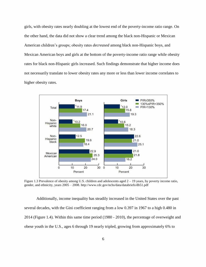
Moreover, poverty rates have also been shown to play a role in obesity trends. As Figure

1.3 illustrates, Ogden, et al. (2010), using NHANES 2005-2008, found that although prevalence

of obesity among the nation’s youth decreases as household income increases, the effect of

higher income is heterogeneous across different ethnic groups and genders. As income

decreased, obesity rates exhibited a clear upward trend among white non-Hispanic boys and

1 According to the CDC, “the built environment includes all of the physical parts of where we live and work (e.g.,

homes, buildings, streets, open spaces, and infrastructure).”

http://www.cdc.gov/nceh/publications/factsheets/impactofthebuiltenvironmentonhealth.pdf

6

girls, with obesity rates nearly doubling at the lowest end of the poverty-income ratio range. On

the other hand, the data did not show a clear trend among the black non-Hispanic or Mexican

American children’s groups; obesity rates decreased among black non-Hispanic boys, and

Mexican American boys and girls at the bottom of the poverty-income ratio range while obesity

rates for black non-Hispanic girls increased. Such findings demonstrate that higher income does

not necessarily translate to lower obesity rates any more or less than lower income correlates to

higher obesity rates.

Figure 1.3 Prevalence of obesity among U.S. children and adolescents aged 2 – 19 years, by poverty income ratio,

gender, and ethnicity, years 2005 – 2008. http://www.cdc.gov/nchs/data/databriefs/db51.pdf

Additionally, income inequality has steadily increased in the United States over the past

several decades, with the Gini coefficient ranging from a low 0.397 in 1967 to a high 0.480 in

2014 (Figure 1.4). Within this same time period (1980 - 2010), the percentage of overweight and

obese youth in the U.S., ages 6 through 19 nearly tripled, growing from approximately 6% to

7

17% (Ogden et al., 2010). These statistics are indicative of an alarming trend among United

States’ youth.

Figure 1.4 Gini Ratios for Households,1968-2013 U.S. Census Bureau, Historical Income Tables: Income Inequality,

https://www.census.gov/hhes/www/income/data/historical/inequality/.

Income inequality may lead to poor physical and mental health because it creates “status

anxiety.” Since income inequality establishes a hierarchy among people, it increases status

competition and causes stress, which in turn leads to negative consequences for one’s health and

longevity (Rowlingson, 2011; R. G. Wilkinson and Pickett, 2009). Among adolescents in

particular, high levels of stress, more commonly found in lower socioeconomic groups, was

shown to be associated with increased odds of developing obesity (Anderson, et. al., 2006;

Goodman and Whitaker, 2002). In addition, the levels of adult and childhood obesity are higher

in countries where income differences are greater (Offer et al., 2012; R. Wilkinson and Pickett,

2009). Finally, the low socioeconomic status of an individual’s parents may negatively affect

health due to stress in the womb and early life (Ravelli et al., 2007; R. Wilkinson and Pickett,

2009).

8

There is some disagreement among researchers regarding the magnitude and direction of

the effect of income equality on adolescent BMI. In the United States, there is evidence (Akee et

al., 2013; Egger et al., 2012; Lee et al., 2014; Shih et al., 2013) that individuals who live near the

bottom of the income distribution, quite often use their limited resources to purchase low-cost,

high-calorie/low-nutrient foods, resulting in a caloric imbalance where intake exceeds output,

thus raising BMI over time. Conversely, Wang and Zhang (2006) find a diminishing correlation

between socio-economic status and adolescent obesity using NHANES data from 1971 to 2002.

My examination of the relationship between income inequality and adolescent obesity will use

three different measures of income equality: the state Gini Coefficient, top 10% income share by

state and top1% income share by state. To the best of my knowledge, this relationship has not

been explored using YRBSS data on adolescent obesity.

Geographic location is another factor that has influenced childhood obesity in the U.S.

Figures 1.5 and 1.6 illustrate findings by Bethell, et al. (2010), who used data from the National

Survey of Children’s Health for 2003 and 2007, and showed that after controlling for a child’s

socioeconomic status, a child’s state of residence had a significant, independent effect on obesity

status. According to their study, between 2003 and 2007, some states experienced increases in

childhood obesity prevalence while others saw the trend decrease. States that had a rise in the

obesity trend included a modest 0.3% in Louisiana to a substantial 13.4% in Mississippi.

Conversely, the variation of childhood obesity prevalence decline among states ranged from

0.2% in Texas to 6.9% in South Dakota (National Survey of Children’s Health, n.d.).

9

Figure 1.5: 2005 Rates of Overweight and Obese Children; http://childhealthdata.org/browse/rankings

Figure 1.6: 2007 Rates of Overweight and Obese Children; http://childhealthdata.org/browse/rankings

10

This research provides additional insight into the origin of the geographic variation in

obesity rates between the U.S. states. Previous research has looked at a myriad of factors in an

effort to explain the variation in childhood obesity prevalence, including the differences in built

environments, maternal employment, food prices, agriculture policies, and technology. This

dissertation contributes to the literature by examining the hypothesis that state-level school

wellness policies also played a role in determining the rates of childhood obesity.

Such a hypothesis is plausible due to a number of reasons: first, schools have the

potential to play a unique role in shaping a student’s diet and exercise related attitudes and

behaviors. On average, K-12 students spend 6.6 hours per day and 180 days per year in school

(Snyder and Dillow, 2012). Additionally, national data show that foods eaten at school contain

19% to 50% of students’ total daily energy intake (Gleason and Suitor, 2001). Since adolescents

spend such a significant portion of their waking hours and consume a considerable portion of

their daily calories in school, it follows that intervention in school environments may be an

effective policy tool in reducing the prevalence of adolescent obesity. By helping adolescents

make healthy food choices and be more physically active, the excess caloric imbalance, which

over time leads to obesity, may be reduced. Moreover, given that obese adolescents are at

increased risk of becoming obese adults, it is essential that prevention strategies be implemented

at a younger age in order to reduce the overall prevalence of obesity and its associated costs to

society (Biro and Wien, 2010; Serdula et al., 1993; Whitaker et al., 1997).

11

In order to address the adolescent obesity epidemic, researchers should look to their

learned behaviors and living environments as they are related to nutrition and physical activity in

order to determine the contributing factors and potential solutions to the epidemic. Policies

directing the development and implementation of interventions that affect adolescent nutrition

and physical activity environments can have a significant impact on the prevalence of adolescent

obesity. Given that youth spend a majority of their waking hours in school, policies directed at

their nutrition and physical activity environments while on the school campus can have a

considerable impact on the adolescent obesity epidemic (Snyder and Dillow, 2012).

2.1 Physical and Social Impact of Adolescent Obesity

There are numerous studies that illustrate the negative effect of obesity on an

adolescent’s health and well-being. For example, obese adolescents experience chronic physical

health conditions, such as Type 2 diabetes, sleep apnea, fatty liver disease, and cardiovascular

disease due to high blood pressure and high cholesterol (Dietz, 1998). The alarming fact is that

historically, the above mentioned diseases had previously only been associated with adults (Katz,

2009; Reilly and Kelly, 2011). Adolescents are also subject to the social stigma of obesity, which

oftentimes leads to exclusion amongst their peers, depression, and low self-esteem (Schwartz and

Puhl, 2003; Strauss and Pollack, 2003). Moreover, overweight and obese adolescents often

experience lower academic performance resulting in lower human capital attainment in

adulthood (Ding et al., 2009; Sabia, 2007).

12

2.2 Economic Costs of Adolescent Obesity

There are also significant economic costs and externalities associated with the treatment

of adolescent obesity-related disease. Obesity and its associated comorbidities raise medical

expenditures and put stress on the health care system (Trasande and Chatterjee, 2009). Medical

costs of obesity account for approximately 10% of total medical expenditure (Finkelstein et al.,

2009). Furthermore, increased adolescent obesity was found to be correlated with both increased

health care utilization and an increase in medical cost (Trasande and Chatterjee, 2009).

Specifically, as shown in Trasande and Chatterjee (2009), elevated BMI (above the 84th

percentile) in 6 - 19 year olds is associated with an increased use of prescription drugs,

emergency room visits, and outpatient visits totaling $14.1 billion in additional medical

expenditure. These are not however, the only costs associated with obesity. In adults, obesity

contributes to poor health which in turn, has been shown to lead to increased disability payments

and decreases in work output due to both absenteeism (missed work days) and presenteeism

(lower productivity while on the job). Burkhauser and Cawley (2004) found the relative risk of

receiving disability income support due to obesity was 5.64 and 6.92 percentage points higher for

women and men, respectively, compared to non-obese individuals. Finkelstein et al. (2005),

reported that indirect costs associated with obesity-attributable absenteeism in the United States

ranged from $77 to $1,033 per obese individual per year, depending on gender and obesity

category.

13

In terms of lost productivity per obese person, Frezza et al. (2006) found that in New

Mexico alone, the cost of obesity was estimated to be $1.5 billion in lost output (including lost

jobs and lost tax revenue), or approximately $3,995 per obese person. Ricci and Chee (2005)

estimated the total value of lost productive time (LPT) at work to be $11.7 billion per year

among obese workers; approximately $7.8 billion of which is directly related to presenteeism.

The productivity losses and indirect costs of absenteeism, disability, and presenteeism associated

with obesity add to the overall costs borne by individuals and society as a whole. Projected

indirect costs of adolescent obesity associated with lost productivity, disability leave, and

premature mortality, from 2020 to 2050 based on assumptions about current productivity growth

and obesity trends, were estimated to be approximately $208 billion (Lightwood et al., 2009).

Due to the increased current medical costs and future trend of even higher expenditures

resulting from adolescent obesity and its comorbidities, there is an urgent need for the

development of effective obesity prevention strategies. Since overweight and obese adolescents

are at increased risk of adult obesity, prevention is crucial in order to reduce the magnitude of

indirect costs associated with decreased worker productivity in the future.

14

Chapter 3: Background of the Child Nutrition and WIC Reauthorization Act of 2004

The Child Nutrition and WIC2 Reauthorization Act of 2004 (CNRA) federal mandate

required all public K-12 schools that received funding for federally reimbursable meal programs

to directly address the school factors listed in Table 1.1 in their school wellness policies prior to

the start of the 2006-2007 school year. The penalty for school districts that failed to comply with

this mandate was the potential loss of their federal funding.

In a review of school policies to promote healthy eating and physical activity in schools,

Story et al.(2009) discuss the CNRA. They find that although the policy directive was a step in

the right direction towards the prevention of childhood obesity, there was a large amount of

variation in schools’ wording of the policies due to the weakness of the mandate in not setting

minimum national standards for the policy components. Most of the current school wellness

policy research reports data regarding compliance with the mandate and strength of the policies

(Longley and Sneed, 2009; Moag-Stahlberg et al., 2008). Metos and Nanney (2007) found that

approximately 78% of state school districts complied with the mandated written policy.

However, the power of the language contained within the policies varied significantly. Similarly,

a report published by Bridging the Gap, a Robert Wood Johnson Foundation program, found that

three years following the mandate enactment, the percentage of students attending school in a

2 According to the USDA, “the Special Supplemental Nutrition Program for Women, Infants, and Children (WIC)

provides Federal grants to states for supplemental foods, health care referrals, and nutrition education for low-

income pregnant, breastfeeding, and non-breastfeeding postpartum women, and to infants and children up to age

five who are found to be at nutritional risk.” http://www.fns.usda.gov/wic/women-infants-and-children-wic

15

district compliant in wellness policy rose from 81% to 99% (Chriqui et al., 2010). Although

compliance was high, the average strength of the wording (rated as strong, weak, or nonexistent)

among school districts in 47 states was a mere 33 out of 100 points.

Other studies have focused on implementation of the policy and whether or not there was

a change in student’s behavior. Lambert et al. (2010) found among elementary teachers

representing 30 schools in Mississippi, that although 85.5% supported the wellness policy

concept, only 59.7% thought that the policies had a positive influence on student health. One of

the key factors to successful implementation of the CNRA was the assignment of a dedicated

wellness coordinator. In a study of school districts in Pennsylvania, Probart et al. (2010) found

that 92% of school districts had complied with the requirement of identifying an individual who

had ultimate responsibility for policy implementation. However, only 28% had a dedicated

wellness coordinator, perhaps implying that wellness policy responsibilities had been given to

school staff and faculty in addition to their other job duties.

Less research has been done that evaluates the effect of the CNRA on the prevalence of

adolescent obesity. Coffield et al. (2011) used self-reported weight and height data taken from

adolescent driver license data in Utah in order to construct their dependent BMI variable. The

analysis of each of their three models showed stronger policies containing more wellness policy

components were correlated with significantly decreased odds of obesity. Conversely, utilizing

data from the 2007 National Survey of Children’s Health, Riis et al. (2012) found that stricter

state school nutrition and physical activity policies were associated with greater odds of obesity,

suggesting that states with high obesity prevalence responded to their health crises with

increased policy implementation efforts.

16

While adolescent obesity is the result of many factors, very little research focuses on

evaluating multidimensional prevention strategies. Although the literature appears to support a

positive effect of the school environment and wellness policies on the prevalence of adolescent

obesity, most studies address only one aspect of policy, such as nutrition, or physical activity.

Thus, there is a significant gap in our knowledge of the impact of these prevention strategies.

I explore the effects of CNRA on adolescent obesity rates. I investigate whether some U.S.

states’ policies were more effective in slowing, or reversing, the prevalence of adolescent obesity

as a result of the CNRA. I examine the effect of the different components of the CNRA on

adolescent’s obesity rates and I evaluate each component’s contribution to reduction in the

obesity rates. Although the CNRA required a written policy to be in place, the mandate did not

specifically address how policies were to be implemented nor evaluated. Consequently, it

facilitated a high level of compliance with the written wellness policies, while setting no

standards regarding measurement of their effectiveness. The estimation model that follows will

explore the direction and magnitude of the effect of these state school wellness policies on

adolescent BMI.

17

Table 1.1: Overview of the Child Nutrition and WIC Reauthorization Act of 2004

Health education Goals for nutrition and health education

Physical education and

activity

Goals for physical education and activity

Nutrition services Guidelines for federal reimbursable meals meeting established

U.S. Department of Agriculture (USDA) regulations and for all

foods available on school campuses during the day

Faculty and staff health

promotion

Designation of one or more individuals responsible for measuring

the implementation of the wellness policy; involvement of school

food authorities and school administrators in developing wellness

policies

Family and community

involvement

Involvement of parents, and the public in developing wellness

policies

http://www.yaleruddcenter.org; CDC - NPAO - Local School Wellness Policy - Adolescent and School Health, 2013

18

Chapter 4: Literature Review

4.1 Obesity and Rational Choice Theory

Cutler et al. (2003) demonstrate that, according to basic economic theory, people make

choices that give them greater utility (make them happier) therefore, if they choose to eat more

and exercise less, and in the absence of negative externalities, there is no reason to intervene with

policy to reduce obesity. We model the decision making behavior of adults as rational; adults are

viewed as making informed decisions, subject to their time and budget constraints, while

maximizing their utility, or sense of well-being. Within this framework, adult obesity can be

modeled as a rational choice that an individual makes, having weighed the benefits (of current

consumption of calories) against the costs (of current and discounted future health consequences)

of their actions. There is however, according to Cawley (2010), “an abundance of precedents for

treating children differently than adults on the basis of their inability to make responsible

decisions: cigarette and alcohol sales to minors are banned; those under age 16 may not drive;

and those under 18 may not vote.” Children and adolescents are not seen as rational individuals

due to their inability to weigh the future costs of their actions; it is this failure of the rationality

assumption that justifies the case for interventions designed to reduce adolescent obesity.

Moreover, in the case of adolescent obesity, adolescents seldom purchase their own food or

decide what their daily meals will consist of either at home or at school (Anderson et al., 2003).

Quite often, an adolescent’s diet and time allocated to physical activity is dictated by the choices

19

their parents make for them. Using micro-level data from the 1984-1999 Behavioral Risk Factor

Surveillance System, Chou et al. (2004) find evidence of the association of change in dietary

behaviors in the United States with the proliferation of fast food restaurants. Further research by

Anderson et al. (2003) shows that over the past thirty years, the increase in maternal labor force

participation, explains 12% to 35% of the increasing childhood obesity trend among families of

high socio-economic status. As a result of the scarcity and increased value of their time,

incentives exist for families to turn to the relatively lower cost convenience of fast foods. The

higher energy (calorie) content and lower nutritional value of these foods is related to the

growing adolescent obesity trend in the United States.

Additionally, current economic research suggests there are negative financial externalities

associated with obesity. Individuals participating in a health insurance pool with other members

who are obese suffer higher premiums than they would otherwise as the increased costs

associated with treatment of obesity’s comorbidities are spread out over the entire group

(Bhattacharya and Sood, 2007). In a New England Journal of Medicine study, researchers found

that the probability of a young child growing up to become an obese adult was approximately

24% if neither parent was obese, but rose to 62% if even one parent was obese (Whitaker et al.,

1997). Evidence of such an inherent problem provides economic rationale for preventing obesity

from the youngest age possible in order to minimize the potential negative externality costs.

Other contributing factors discussed in the literature include: genetic variations (e.g.

race/ethnicity, gender, age), maternal behavior during a child’s formative years, family food

environment, family socioeconomic status, technology, and the physical environment (e.g.

access to recreational facilities). The origin of obesity however, is primarily due to an energy

imbalance where calorie consumption exceeds calorie expenditure. The growing consumption of

20

high calorie, low nutrient, inexpensive processed foods along with a sedentary lifestyle combine

to result in the growing obesity trend in the United States. An excess consumption of calories on

a daily basis will result in weight gains which, if left unchecked, over time will lead to an

increased probability of obesity. Recent economic research, focused on identifying the potential

determinants of this imbalance, offers useful insights into changes that have taken place in our

environment that may have given individuals incentive to consume more calories, expend fewer

calories, or some combination of the two, thus contributing to the rise in obesity in general (Chou

et al., 2004; Cutler et al., 2003; Lakdawalla and Philipson, 2002; Philipson and Posner, 1999).

Cutler et al. (2003) find that technology advances in the past three decades such as:

vacuum packing, preserving, deep freezing, and microwaving have enabled the consumption of

high calorie, low nutritive value, mass produced foods at a lower cost to consumers relative to

foods prepared at home. Harris et al. (2007), using nationally representative data from the

ACNielsen Homescan panel, confirm the increased use of convenience foods in U.S. homes

today. They found a positive and significant relationship between households with children and

additional spending on convenience foods thus asserting the earlier conclusion by Cutler et al.

(2003); a considerable amount of food preparation has shifted from in-home to food

manufacturers.

Cawley (2010) summarizes the aforementioned determinants by stating that, “it is not

practical or desirable to lower childhood obesity by turning back the clock or reversing these

trends.” Asking society to stop developing and using food technology, causing food prices to rise

in the hopes that the effect will lead to decreased calorie consumption is folly.

21

The same is true of women in the labor force; the notion that today’s society would even

consider a decrease within a workforce comprised of more than 45% females is imprudent.

Similar logic can be applied to the multiple contributory factors of adolescent obesity. Rather

than looking to the past, policymakers’ time would be better spent focusing on obesity

prevention strategies that address the negative repercussions of the gains that society has made to

date.

4.2 Obesity and Behavioral Economics

Behavioral economics literature argues that obesity is not a rational choice (Chou et al.,

2004; Council on Communications and Media, 2011; Zimmerman, 2011). Zimmerman (2011)

suggests that it is not the result of individual utility maximization given fixed preferences, but

rather the outside influence of food producers who alter their products in such a way as to sway

individual tastes towards unhealthy, high-calorie, low-nutrient foods. Moreover, a 2012 report

published by the Institute of Medicine (IOM) concluded that in order to have a positive effect on

the systemic, complex obesity problem, a significant societal change must take place. They

advocate a paternalistic approach of government interventions that might “nudge” individuals

towards better choices that would be more in the best interests for their health (Institute of

Medicine (U.S.) and Glickman, 2012).

4.2.1 The Case for Paternalism

There are two main categories of systematic bias in individual behavior: cognitive bias

and persistent self-control problems. Cognitive bias occurs when individuals prefer to follow the

status-quo rather than search for alternatives that may improve their well-being.

22

Hendrickse et al. (2015), found support for this bias in a study of how food images triggered

study individual’s appetites, which in turn led to food cravings and eventual overeating.

Persistent self-control problems in obese individuals are displayed in their regular inconsistency

in discounting the future poor health trade-offs between their present and future selves.

Some school interventions that have shown potential in addressing both forms of bias in

students who purchase their meals in school cafeterias are: placing fruit rather than high-calorie,

high-fat snacks in more accessible areas, placing salad bar stations in a more central location

than other food stations, and requiring that candy and soda be paid for in cash rather than with

lunch card credits (Just et al., 2007).

Given that traditional economic theories do not do a very good job of explaining

individual behavior, behavioral economics and a more paternalistic approach offers considerable

prospects for researching the obesity issue from a different perspective. By assuming that

individuals are not making choices in their own best interest, there are a considerable number of

potential policy interventions other than, for example, influencing prices through the use of “sin

taxes” designed to steer individuals away from goods that are considered harmful to them or

increasing the amount of information available, such as showing calorie counts on menus.

4.3 Adolescent Obesity and Public Policy Intervention

While there is widespread agreement that obesity is a priority health concern in the

United States, there is considerable disagreement as to whether and to what extent government

should intervene with policies that are designed to affect the poor health choices made by

overweight and obese consumers. Adolescent obesity can, however, benefit from the guiding

principles of economics that support interventions in the case of such market failures, such as

23

irrational behavior, externalities, and lack of information. Cawley (2010) suggests that the

objective of obesity prevention policy should not be to set subjective goals, such as a particular

level of obesity in society. Interventions should be established so that they correct market

failures, thus allowing the “right” level of obesity to be reached in the most cost-effective

manner possible.

In order to target the “right” level of adolescent obesity in this manner, interventions

designed to address adolescent’s lack of “rationality” through modifying their eating and

physical activity behaviors while in school, can play a key role in reversing the upward trend. In

school, administrators and teachers acting in loco parentis can help to instill healthy behaviors in

their students by educating them and regulating their school environment. If school staff and

faculty are provided with resources that allow the design and application of policies that outline

specific, measureable goals and implementation procedures for student wellness, it is possible

that the high tide of childhood obesity prevalence can be turned. Economic research on the

prevalence of adolescent obesity discusses not only school wellness policies in general, but also

the effect of individual policy components such as federally funded school meal programs and

availability of competitive foods on school campuses.

Results pertaining to the correlation of participation in federally funded free and reduced-

price school lunches and childhood weight gain are mixed in the economic literature.

Schanzenbach (2009), utilizing a regression discontinuity design in order to study children at

either side of the income eligibility cutoff for school lunch subsidies, found a significant positive

correlation with increased obesity rates. Using panel data from the Early Childhood Longitudinal

Study – Kindergarten Cohort (ECLS-K) that followed approximately 15,000 students from 1,000

different schools from kindergarten through eighth grade, Schanzenbach (2009) found the

24

increased calories consumed by students eligible for the free and reduced price lunch programs

could lead to a two percentage point increase in obesity rates. Millimet et al. (2010) extend this

research in order to control for the effects of selection into and participation in either the School

Breakfast Program (SBP) and/or the National School Lunch Program (NSLP) on child obesity.

The results of conditioning on SBP participation and allowing for positive selection into the SBP

showed that the increase in child obesity rates was primarily the result of the NSLP, thus

confirming Schanzenbach’s earlier findings and also providing valuable information regarding

the benefits of the SBP as well as a clear need to investigate the detrimental effects of the NSLP.

While school officials endeavor to provide nutritious meal choices in main dining areas,

they also face the reality of annual budget gaps. In order to supplement their funding, many

schools turn to offering “competitive foods” (foods and beverages sold outside of Federal meal

programs, regardless of nutritional value). Kubik et al. (2005), in a cross-section study of middle

school students in Minneapolis, Minnesota, found that school food practices that allowed access

to competitive foods throughout the school day was associated with increased BMI rates.

Although schools in the United States receive an estimated $750 million a year from companies

that sell snacks and beverages (Egan, 2002), it is essential that they consider the nutritive value

of the foods being offered. Already, many schools have taken it upon themselves to improve

their competitive food offerings with little loss of revenue (Wharton et al., 2008).

25

Chapter 5: Conceptual Framework

Utilizing rational choice theory, this research will empirically test the relationship

between state school wellness policies and adolescent obesity. According to rational choice

theory, an individual’s behavior is the result of that individual choosing the behavior that best

maximizes their satisfaction, given that they are well informed of all alternatives and potential

consequences of their actions (Simon, 1955). In economics, we assume that these individuals are

rational in that they are able to weigh the discounted value of any future consequences against

the benefits of their present choices (Becker and Murphy, 1988). The choices that these rational

individuals make are subject to time and money constraints and they are assumed to allocate

these resources in such a way that their utility, or satisfaction, is maximized.

A practical application of rational choice theory is Grossman’s (1972) demand for good

health in which individuals begin their lives with a certain health stock which depreciates over

time until death occurs. Over the course of their lifetime, individuals can choose to consume

goods and services that produce “health,” subject to their time and budget constraints, in order to

invest in their health stock, so that depreciation is slowed and their length of life extended. Since

I am exploring adolescent obesity, and many of the decisions that affect an adolescent’s health

and body weight are made by parents as well as individuals acting in loco parentis, this research

will employ a slightly modified version of an extended Grossman model, introduced by Lena

Jacobson, that looks at the family as producers of health rather than the individual (Jacobson,

2000).

26

The extended Grossman model begins with a family utility function

𝑈 = 𝑈(𝐻𝑚, 𝐻𝑓 , 𝐻𝑎, 𝑍)

where the family’s utility is a function of the mother’s and father’s health, 𝐻𝑚, 𝐻𝑓, respectively,

the adolescent’s health, 𝐻𝑎, and consumption of other goods, Z.

The adolescent’s health depreciates over time according to

𝜕𝐻𝑎𝜕𝑡

⁄ = 𝐼𝑎 − 𝛿𝑎H𝑎

where 𝐼𝑎 are investments in the adolescent’s health and 𝛿𝑎 is the depreciation of the adolescent’s

initial health stock, 𝐻𝑎.

According to Jacobson, the adolescent’s health investments, 𝐼𝑎, are produced by the

parent’s use of their own time with the child and choice of market goods for the child. The

investment in a child’s health is thus produced according to the production function

𝐼𝑎 = 𝐼𝑎(𝑀𝑎, ℎ𝐻𝑎,𝑚, ℎ𝐻𝑎,𝑓; 𝐸𝐻,𝑚, 𝐸𝐻,𝑓)

where ℎ𝐻𝑎,𝑚 and ℎ𝐻𝑎,𝑓 represent the time spent in producing adolescent health by mother and

father, respectively; 𝐸𝐻,𝑚and 𝐸𝐻,𝑓 are efficiency parameters (i.e. parent level of education) that

may affect production of health; and finally, 𝑀𝑎 , where

𝑀𝑎 = 𝑀𝑎𝑝𝑢𝑏𝑙𝑖𝑐 + 𝑀𝑎

𝑝𝑟𝑖𝑣𝑎𝑡𝑒

which represents the adolescent’s consumption of goods 𝑀𝑎𝑝𝑢𝑏𝑙𝑖𝑐

(school) and 𝑀𝑎𝑝𝑟𝑖𝑣𝑎𝑡𝑒

(all other

goods). In this research, an adolescent’s production of health, 𝐼𝑎, is based not only on parental

choices of their consumption and time allocation, but also through school officials acting in loco

parentis for adolescents who attend public schools. Thus, the final model is

𝐼𝑎 = 𝐼𝑎(𝑀𝑎𝑝𝑢𝑏𝑙𝑖𝑐 + 𝑀𝑎

𝑝𝑟𝑖𝑣𝑎𝑡𝑒 , ℎ𝐻𝑎,𝑚, ℎ𝐻𝑎,𝑓; 𝐸𝐻,𝑚, 𝐸𝐻,𝑓).

27

The relationship between all inputs in the production of a child’s weight is illustrated in Figure

1.7, where both parents and school play a role in determining a child’s nutrition, physical

activity, nutrition education, and physical education, and both parents and school will have an

impact on caloric consumption and expenditure.

Figure 1.7: Child caloric consumption/expenditure influences

28

Chapter 6: Research Methodology

6.1 Model Specification

The model I estimate takes on the following form:

𝐵𝑀𝐼𝑖𝑠𝑡 = 𝛽0 + 𝛽1𝑋𝑖𝑠𝑡 + 𝛽2𝑍𝑖𝑠𝑡 + 𝛽3𝐶𝑖𝑠𝑡 + 𝛽4𝑊𝑒𝑙𝑙𝑃𝑜𝑙𝑖𝑐𝑦𝑖𝑠𝑡 + 𝛽5𝑆 + 𝜇𝑖𝑠𝑡

where 𝐵𝑀𝐼𝑖𝑠𝑡 represents the body mass index measure for adolescent i in state s at time t; 𝑋𝑖𝑠𝑡 is

a vector of child characteristics; 𝑍𝑖𝑠𝑡 is a vector of state-level adult characteristics; 𝐶𝑖𝑠𝑡 is a vector

of state-level contextual characteristics; WellPolicy is a measure of the state wellness policy; S

represents state dummies; and finally, 𝜇𝑖𝑠𝑡 represents unobservable factors that are uncorrelated

with the rest of the independent variables.

6.2 Dependent Variable

As the output for an adolescent’s health production function that contributes to overall

family utility, I use Body Mass Index (BMI), a measure of obesity. BMI is the generally

accepted measure used to describe weight status (underweight, healthy, overweight, and obese)

for adults3 however, due to the different growth rates between children and adolescents of

3 According to the CDC, BMI is calculated by dividing weight in pounds (lbs) by height in inches (in) squared and

multiplying by a conversion factor of 703.

http://www.cdc.gov/healthyweight/assessing/bmi/adult_bmi/index.html#Interpreted

29

different age and gender, the BMI calculation is compared to the CDC’s gender-specific BMI-

for-age growth charts (Figures 1.8 and 1.9) to determine weight status.

Table 1.2 shows the range of weight status categories for an adolescent who is below the

5th percentile on the CDC BMI-for-age growth chart (underweight) to above the 95th percentile

(obese). For example, a 15 year old girl with a calculated BMI of 27 would fall between the 90

and 95th percentile on the CDC BMI-for-age growth chart for girls, thus placing her in the

overweight category.

Table 1.2: CDC BMI-for-age weight status categories and corresponding percentiles

Weight Status Category

Percentile Range

Underweight

Less than 5th percentile

Healthy weight

5th percentile to less than 85th percentile

Overweight

85th percentile to less than 95th percentile

Obese

Equal to or greater than 95th percentile

http://m.cdc.gov/en/HealthSafetyTopics/HealthyLiving/HealthyWeight/AssessingYourWeight/BodyMassIndex/BMIChildrenTeens

30

Figure 1.8: CDC BMI-for-age growth chart for girls

http://www.cdc.gov/growthcharts/data/set1clinical/cj41c024.pdf

Figure 1.9: CDC BMI-for-age growth chart for boys

http://www.cdc.gov/growthcharts/data/set1clinical/cj41c024.pdf

31

6.3 The Primary Explanatory Variable

The primary explanatory variable of interest are the state school wellness policies that

direct school officials’ behavior as it relates to actions that may have an effect on adolescent

health.

According to the OECD, composite indicators are seen as beneficial tools in providing a

point of reference for country performance post-policy implementation as well as analyzing and

formulating public policy performance across countries. They are useful for simplifying often

complex, multi-dimensional policies and to help understand trends in both individual indicators

and across countries and/or regions (Joint Research Centre-European Commission and others,

2008). Following the methodology outlined in the OECD’s Handbook on Constructing

Composite Indicators, I constructed an index that was used to: (1) develop a composite indicator

based on elements of state school wellness policies that may impact adolescent obesity, (2)

establish a benchmark measure of each state’s performance in complying with the goals of the

CNRA, (3) apply the indicator in order to describe the differences in adolescent BMI over time

and across states, and (4) to determine the importance of the individual components of the index.

6.4 Other Explanatory Variables

Other individual-level explanatory variables included age, gender, race, and how many

days per week the student participated in PE class. To control for state-level contextual effects, I

included the state adult obesity rate, percent of the state population with a bachelor’s degree, the

state poverty rate, the state violent crime rate, and a measure of income inequality.

Income inequality was measured in one of three ways: 1) state-level Gini coefficient, 2)

the concentration of income in a state’s top 10 percent of income earners, and 3) the

32

concentration of income in a state’s top 1 percent of income earners. The Gini coefficient is the

most commonly used measure of income inequality; it measures the extent to which income

distribution among individuals deviates from a perfectly equal distribution with 0 representing

perfect equality and 1 representing perfect inequality. A positive a positive sign on the

regression coefficient of the Gini variable would indicate that income inequality leads to an

increase in the BMI measure. The last two measures are income shares of the top 1 and top 10

percent of earners as a percentage of national income. A positive association between these

variables and the BMI measure would imply that income inequality increases adolescent BMI.

To control for the fact that I am unable to observe whether an individual attends public

or private school, I included the percent of the state’s high school student population attending

either public or private school. State dummy variables were added to control for unobserved state

specific factors affecting individual student BMI (availability of outdoor park spaces for physical

activity, number of grocery stores with fresh produce available, and number of fast food

restaurants). Finally, I used year dummy variables to account for time-specific unobserved

determinants of BMI. Table 1.3 summarizes all explanatory variables used in this research.

Correlations for individual-level and state-level explanatory variables are shown in appendix

tables A.1 and A.2, respectively.

33

Table 1.3: Explanatory Variables Used in Regression Analysis Variable Description

Age

Discrete, age in years

Female

Dummy variable =1 if female, =0 otherwise

Black Dummy variable =1 if Black, = 0 otherwise

Asian Dummy variable =1 if Asian, =0 otherwise

Hispanic Dummy variable =1 if Hispanic, = 0 otherwise

Other Dummy variable =1 if American Indian/Alaskan native, Hawaiian / Pacific Islander,

Multiple-Hispanic, or Multiple – Non-Hispanic, =0 otherwise

Days in PE Discrete, how many days in a week the individual participates in school PE class

Wellness Policy

Index

Continuous, index value of the state from which the individual observation comes

Adult Obesity Rate Continuous, adult obesity rate of the state from which the individual observation comes

College Education Continuous, college education attainment of the state from which the individual

observation comes

Poverty Rate Continuous, poverty rate of the state from which the individual observation comes

Violent Crime Rate Continuous, violent crime rate of the state from which the individual observation comes

Gini coefficient Continuous, Gini coefficient of the state from which the individual observation comes

Top 10% Continuous, income share of top 10 % income earners of the state from which the

individual observation comes

Top 1% Continuous, income share of top 1 % income earners of the state from which the

individual observation comes

Public School Rate Continuous, public school attendance rate of the state from which the individual

observation comes

Private School Rate Continuous, private school attendance rate of the state from which the individual

observation comes

Year

Dummies indicating the year individual is observed

State

Dummies controlling for the state from which the individual observation comes

34

Chapter 7: Data Sources

The data for this research come from the following sources: (1) the Youth Risk Behavior

Surveillance System (YRBSS); (2) the School Health Policies and Practices Study (SHPPS); (3)

U.S. Census Bureau; (4) National Center for Chronic Disease Control and Prevention (CDC);

and (5) the U.S. State-Level Income Inequality Data Series published and maintained by Mark

W. Frank.

.

7.1 Youth Risk Behavior Surveillance Survey

The Youth Risk Behavior Surveillance System (YRBSS), conducted biennially since

1991, is a nationally representative survey of high school students (grades 9–12) that was

established by the CDC to monitor the prevalence of risky youth behaviors, including those

relating to physical activity and obesity. The level of identification is both at the state and district

level. However, the district level data collection was only funded for 22 large urban areas.

Variables used from the YRBSS included: age, gender, ethnicity, weight, height and the

average number of days per week a student participated in physical education (PE) classes at

school. Weight and height are self-reported in the YRBSS and are therefore likely reported with

error. The nature of this reporting error in the YRBSS is unknown, because the true height and

weight of YRBSS respondents is not observed. In order to determine the magnitude of reporting

error in weight among high school students, researchers at the CDC surveyed high school

students and collected data on both self-reported and measured weight and height.

35

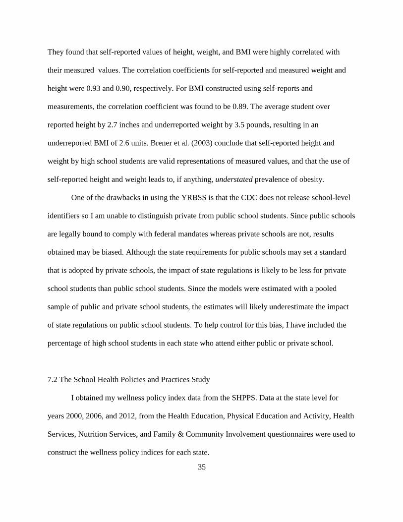
They found that self-reported values of height, weight, and BMI were highly correlated with

their measured values. The correlation coefficients for self-reported and measured weight and

height were 0.93 and 0.90, respectively. For BMI constructed using self-reports and

measurements, the correlation coefficient was found to be 0.89. The average student over

reported height by 2.7 inches and underreported weight by 3.5 pounds, resulting in an

underreported BMI of 2.6 units. Brener et al. (2003) conclude that self-reported height and

weight by high school students are valid representations of measured values, and that the use of

self-reported height and weight leads to, if anything, understated prevalence of obesity.

One of the drawbacks in using the YRBSS is that the CDC does not release school-level

identifiers so I am unable to distinguish private from public school students. Since public schools

are legally bound to comply with federal mandates whereas private schools are not, results

obtained may be biased. Although the state requirements for public schools may set a standard

that is adopted by private schools, the impact of state regulations is likely to be less for private

school students than public school students. Since the models were estimated with a pooled

sample of public and private school students, the estimates will likely underestimate the impact

of state regulations on public school students. To help control for this bias, I have included the

percentage of high school students in each state who attend either public or private school.

7.2 The School Health Policies and Practices Study

I obtained my wellness policy index data from the SHPPS. Data at the state level for

years 2000, 2006, and 2012, from the Health Education, Physical Education and Activity, Health

Services, Nutrition Services, and Family & Community Involvement questionnaires were used to

construct the wellness policy indices for each state.

36

The SHPPS is the largest, most comprehensive examination of school health policies in

the United States (Kann et al., 2007). Since 1994, the study has been completed every six years

in collaboration with the Division of Adolescent and School Health (DASH), and the CDC.

According to a Division of Adolescent and School Health article (2011), the purpose of SHPPS

is to “assess school health policies and practices at the state, district, school, and classroom

levels.” School sampling was intended to recruit a nationally representative sample based on

urban city, SES4, school level (e.g, elementary, middle, and high), and enrollment size. The final

sample included a total of 1,103 schools from across the United States and reflected a 78%

response rate.

As shown in Table 1.4, a principal component analysis approach was used to group

responses to survey questions into their respective domain of interest that correlated with the

wellness policy mandate criteria. Principal component analysis is a statistical method used for

data reduction purposes by analyzing the relationships among large numbers of variables in order

to group them in terms of their common underlying dimensions or components. This approach

was used to create a composite index that contained variables measuring similar concepts. Since

the variable of interest in this research was the school wellness policy, in order to give a

meaningful interpretation of its estimated coefficient, a single index variable was preferred to

multiple discrete categories.

4 According to the American Psychological Association, “socioeconomic status (SES) is often measured as a

combination of education, income and occupation. It is commonly conceptualized as the social standing or class of

an individual or group.” http://www.apa.org/pi/ses/resources/publications/factsheet-education.aspx

37

Table 1.4: School Health Policies and Practice Study Domains

Domain Description

Health Education

Indicates whether states adopted policy stating that

schools follow national health education standards or

guidelines

Physical Education &

Activity

Indicates whether states adopted policy stating that

schools follow national physical education and activity

standards or guidelines

Nutrition Services Indicates adherence to USDA nutrition standards

Health Services

Characteristics of state-level school health activities (e.g.

health council to guide development and implementation

of school wellness policy)

Family &

Community

Involvement

Describes types of health education offered to families and

level of community involvement in developing school

wellness strategy

http://www.cdc.gov/healthyyouth/shpps/brief.htm

7.2.1 Principal Component Analysis

Principal component analysis (PCA) is a multivariate statistical technique that is used to

reduce the size of a dataset that consists of a large number of correlated variables while retaining

as much of the variation as possible from the original dataset (Jolliffe, 2002). PCA, as introduced

by Pearson in 1901 and later developed by Hotelling (1933), was not widely used until computer

use allowed for computation of the matrix algebra involving more than four variables to be more

tractable. The full potential of PCA has more recently been realized in a variety of empirical

applications in both the physical and social sciences. However, it did not gain popularity as a

means of deriving weights necessary in constructing a linear composite index until Filmer and

Pritchett’s (2001) paper in which they utilize PCA to formulate a linear index proxy for

38

household wealth from asset ownership indicators. This research employs the PCA technique in

order to exploit the variation and to reduce any redundancy that may exist within the SHPPS

data.

Formally, PCA takes a set of k correlated variables 𝑋 = {𝑋1, 𝑋2, … 𝑋𝑘} (such as state

school health policy variables) and transforms them into a new set of uncorrelated variables 𝑍 =

{𝑍1, 𝑍2, … , 𝑍𝑘} called principal components, each of which is an independent, linear weighted

combination of the initial variables as follows:

𝑍1 = 𝑎11𝑋1 + 𝑎12𝑋2 + ⋯ + 𝑎1𝑗𝑋𝑗

.

.

.

𝑍𝑘 = 𝑎𝑘1𝑋1 + 𝑎𝑘2𝑋2 + ⋯ + 𝑎𝑗𝑘𝑋𝑗

where 𝑎𝑗𝑘 is the weight for the kth principal component and the jth variable. The weights (𝑎𝑗𝑘)

for each principal component are derived from the eigenvectors of the correlation matrix and the

variance by the eigenvalue of the corresponding eigenvector. Finally, principal components

(𝑍1, 𝑍2, … , 𝑍𝑘) are arranged so that the first component (𝑍1) accounts for the greatest amount of

variation in the original data. The second component (𝑍2), uncorrelated with the first component,

explains the maximum remaining variance, which is less than the first. All successive

components are uncorrelated with the preceding components and explain less and less of the

variation in the original data.

The assumptions of PCA include: (1) sufficient number of observations, (2) no bias in

selecting individual indicators, (3) strong correlations in the data and (4) multivariate normality.

39

When determining the minimum acceptable sample size in PCA, there are two classes of

recommendations found in the literature; the first states that it is the number of cases

(observations) that is important and the second suggests that it is instead the observation to

variable ratio that is most important. There is little agreement in the literature as to which rule is

best to follow however, in a study by MacCallum et al. (1999), a Monte Carlo experiment

showed excellent results with a sample size of 60 and 20 variables or a 3:1 ratio of observations

to variables. Similarly, the final sample of this paper’s study included 153 observations and 56

variables or a 2.7 to 1 ratio.

Further, as the variables for this study were not selected ad hoc from various different

sources, but instead taken from a specifically constructed survey, there should be little to no bias

among the individual indicators as well as strong correlations within the data. Finally, given that

standard PCA assumes multivariate normality, thus working best with continuous data, this

research follows a technique developed by Kolenikov and Angeles (2009) that utilized

polychoric correlations in the PCA analysis in order to accommodate the discrete nature of the

SHPPS data.

7.2.2 Polychoric Principle Component Analysis Implementation

Prior to implementing the regression analysis, I performed principal component analysis

(PCA) and calculated the wellness policy measures. Jolliffe (2002) suggests using Bartlett’s test

of sphericity and the Kaiser-Meyer-Olkin (KMO) procedures prior to performing principal

component analysis to determine if PCA is an appropriate method for analyzing the data.

40

The null hypothesis of the Bartlett test is that the observed correlation matrix is

significantly different from the identity matrix. In determining the general relationship between

variables, the determinant of the correlation matrix |R| is calculated; under the null hypothesis,

|R| is equal to one whereas if the variables are highly correlated |R| will be closer to zero. The

Bartlett’s test statistic is calculated according to

𝜒2 = − (𝑛 − 1 −2𝑝 + 5

6) × ln|𝑅|

where n is the number of observations, p is the number of variables and R is the correlation

matrix, determines to what extent the data deviate from |R| = 1.

The KMO is a measure used to determine if the sample size is adequate for principal

component analysis. It tests the ratio of partial correlations relative to original correlations in the

sample. If the variables share common factors, the partial correlations should be small and KMO

will be close to 1. The KMO test statistic is calculated according to

𝐾𝑀𝑂 = (∑ ∑ 𝑟𝑖𝑗2) / (∑ ∑ 𝑟𝑖𝑗

2 + (∑ ∑ 𝑎𝑖𝑗2 ))

where aij are the partial correlations.

Analysis was performed in STATA (version 12) using the “polychoric” and

“polychoricpca” commands to estimate the polychoric correlations among pairwise variables

and perform the principal component analysis, respectively. Both the result of the KMO and

Bartlett’s test of sphericty, summarized in Table 1.5 below, indicate that principal component

analysis is an appropriate method for analyzing this data.

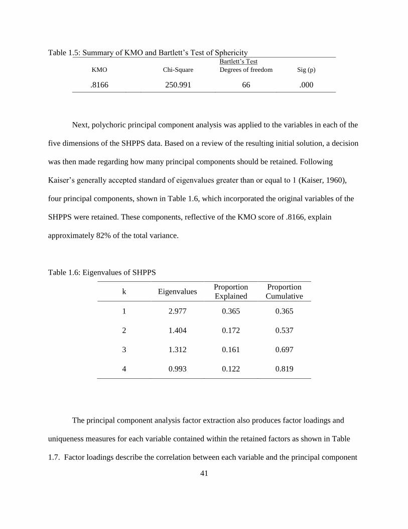
41

Table 1.5: Summary of KMO and Bartlett’s Test of Sphericity Bartlett’s Test

KMO Chi-Square Degrees of freedom Sig (p)

.8166 250.991 66 .000

Next, polychoric principal component analysis was applied to the variables in each of the

five dimensions of the SHPPS data. Based on a review of the resulting initial solution, a decision

was then made regarding how many principal components should be retained. Following

Kaiser’s generally accepted standard of eigenvalues greater than or equal to 1 (Kaiser, 1960),

four principal components, shown in Table 1.6, which incorporated the original variables of the

SHPPS were retained. These components, reflective of the KMO score of .8166, explain

approximately 82% of the total variance.

Table 1.6: Eigenvalues of SHPPS

k Eigenvalues Proportion

Explained

Proportion

Cumulative

1 2.977 0.365 0.365

2 1.404 0.172 0.537

3 1.312 0.161 0.697

4 0.993 0.122 0.819

The principal component analysis factor extraction also produces factor loadings and

uniqueness measures for each variable contained within the retained factors as shown in Table

1.7. Factor loadings describe the correlation between each variable and the principal component

42

factors that have been extracted from the data. To illustrate, the NatlHlthEdStd variable, based on

the SHPPS Health Education Questionnaire survey response to whether or not the state requires

schools to follow a nationally recognized health education curriculum, is highly correlated with

Factor 1, but insignificantly correlated with the other three factors. Similarly, the

OnsiteFastFood variable, based on the SHPPS Health Education Questionnaire survey response

to whether or not states allow brand name fast food service on site, is highly correlated with

Factor 4, but insignificantly correlated with the other three factors.

The uniqueness measure is the part of the variance of the components within each factor

that is “unique” and not shared with other variables. For example, 15.18% of the variance in the

NatlHlthEdStd variables is not shared with other variables in the model. Conversely, the

SchoolCoord variable, based on the SHPPS Health Education Questionnaire survey response to

whether or not states require schools to have a committee, task force, etc. in charge of

coordinating community and family involvement in school health programs, has a higher

uniqueness value where 93.55% of its variance is not shared with other variables in the model.

Since we want the representative variables within each factor to be correlated with one

another, the higher the value of the uniqueness measure, the less relevance it has in the overall

factor model. Variables that loaded the highest on each respective factor are assigned to that

factor (highlighted values in Table 1.7) for constructing the overall wellness policy index

measure for each state.

43

Table 1.7: SHPPS PCA Factor Extraction Results

Survey Variable

National

Standards

(Factor 1)

State

Requirement

(Factor 2)

Screening

(Factor 3)

State

Recommended

(Factor 4)

Uniqueness

Health Education NatlHlthEdStd 0.7572 0.1034 -0.5102 -0.0615 0.1518

Health Education HlthEdrequired 0.0916 0.6333 -0.4941 0.2485 0.2848

Health Services StudentHlthHist 0.1413 0.0457 0.5241 -0.2726 0.4399

Health Services HlthScreening 0.1516 0.2422 0.3859 -0.3953 0.6804

Nutrition Services FoodSvcEduc 0.0284 0.3172 0.1012 0.2108 0.8038

Nutrition Services USDAstdrds 0.7086 -0.0617 0.3449 0.1379 0.3561

Nutrition Services OnsiteFastFood 0.5642 0.0937 0.0857 0.6981 0.1783

Physical Education PEexempt 0.2977 -0.5467 0.6274 -0.2994 0.1293

Physical Education PEactivity 0.7734 -0.4226 0.3990 0.0059 0.064

Physical Education PErequired -0.0031 0.7259 -0.0106 0.0982 0.4633

Family/Community

Involvement FamCommreq -0.0670 0.3239 0.0972 0.0474 0.8264

Family/Community

Involvement SchoolCoord 0.1988 0.1051 0.1169 0.4988 0.9355

44

7.2.3 Constructing the Wellness Policy Indices

Following the principal component estimation and assignment of variables to their

respective factors based on the factor loadings, two wellness policy indices (WPIE and WPIWT)

for each of the three SHPPS policy years (2000, 2006, and 2012) were calculated.

The first index (WPIE) was derived beginning with computation of factor scores (f)

according to

𝑓𝑠𝑡 = ∑ 𝑋𝑖𝑠𝑡

12

𝑖=1

where 𝑓𝑠𝑡represents the factor score for state s in year t and 𝑋𝑖𝑠𝑡 denotes a binary value for state s

in year t, equal to one if the state had a requirement in place for wellness policy variable i, and

zero otherwise.

Next, the equal weight (b) to be applied to each factor score was calculated according to

𝑏 = ∑ 𝐺𝑘

4𝑘=1

4

where k identifies each retained component factor and G represents the associated eigenvalue

obtained from the principal component extraction. Finally, WPIE was calculated according to

𝑊𝑃𝐼𝐸𝑠𝑡 = 𝑏 ∑ 𝑓𝑠𝑡

4

𝑘=1

where 𝑊𝑃𝐼𝐸𝑠𝑡 represents the equal weighted wellness policy index calculation for state s in year

t; b the equal weight measure; and, f the factor score for state s in year t. Results for the equal

weighted index calculation are given in Table 1.9.

45

The second index (WPIWT) was derived as a weighted average (bwt) of the four principal

components that accounted for the proportion of variance explained by each individual

component according to

𝑏𝑤𝑡𝑘 = 𝐺𝑘

∑ 𝐺𝑘4𝑘=1

where k identifies each retained component factor and G represents the eigenvalue obtained from

the principal component extraction. Next, factor scores (fwt) were calculated for each of the four

retained components according to

𝑓𝑤𝑡𝑘𝑠𝑡 = ∑ 𝑋𝑘𝑠𝑡

where 𝑓𝑤𝑡𝑘𝑠𝑡 represents the factor score for principal component k for state s in year t; 𝑋𝑖𝑠𝑡

denotes a binary value for wellness policy variable i that comprises factor component k for state s

in year t and is equal to one if the state had a requirement in place for wellness policy variable or

zero otherwise.

Finally, WPIWT was calculated according to

𝑊𝑃𝐼𝑊𝑇𝑠𝑡 = ∑ 𝑓𝑤𝑡𝑘𝑠𝑡𝑏𝑤𝑡𝑘

4

𝑘=1

where 𝑊𝑃𝐼𝑊𝑇𝑠𝑡 represents the weighted average wellness policy index calculation for state s in

year t; 𝑓𝑤𝑡𝑘𝑠𝑡 the factor score for component k for state s in year t; and 𝑏𝑤𝑡𝑘 the weighted

average measure for each component k. Results for the weighted average index calculation can

be found in Table 1.8.

As shown in Table 1.9, when comparing the outcomes between the methods of wellness

policy calculations, the state rankings were essentially the same (shaded states remained in the

same quintile). Irrespective of the chosen technique, weighting methods are basically based on

46

value judgments (Joint Research Centre-European Commission and others, 2008). For this

reason, and rather than assume that each component of the index is equally significant in the

final index construction, regression analysis utilized results of the weighted average index.

7.3 Other Data

In addition to the YRBSS and SHPPS surveys, I used U.S. Census Bureau data from both

the American Community Survey (ACS) and the Current Population Survey (CPS) to obtain the

percentage of the state population with a bachelor’s degree or higher, the state-level percentage of

high school students attending either public or private school, and the state-level poverty and

violent crimes rates. I also used data from the CDC to obtain adult obesity rates by state. The state-

level Gini coefficient and proportion of top 1 and top 10 income earners for years 1999-2013 came

from U.S. State-Level Income Inequality Data Series published and maintained by Mark W. Frank

(Frank, 2013). These indices were constructed from individual tax filing data from the Internal

Revenue Service.

47

Table 1.8: State wellness policy index results by year and method 2000 2006 2012

State Equal

weight

Weighted

Average

Equal

weight

Weighted

Average

Equal

weight

Weighted

Average

Alabama 9.574 1.882 12.259 2.249 13.930 2.708

Alaska 10.866 2.224 5.154 0.951 16.716 3.436

Arizona 4.253 0.787 9.654 1.946 12.663 2.809

Arkansas 11.423 2.075 7.082 0.947 11.793 2.182

California 11.024 2.034 9.804 1.976 11.281 2.138

Colorado 7.894 1.446 12.621 2.394 8.785 1.930

Connecticut 13.039 2.742 14.209 3.128 16.523 3.538

Delaware 7.522 1.409 10.030 1.890 15.880 3.510

Florida 11.633 2.107 6.687 1.111 9.313 1.761

Georgia 5.015 0.851 9.863 1.436 10.239 1.726

Hawaii 11.701 2.336 15.045 2.991 13.373 2.767

Idaho 7.940 1.147 11.701 1.851 12.203 2.505

Illinois 9.415 1.353 11.202 2.096 12.609 2.507

Indiana 12.917 2.727 11.648 2.176 12.020 1.972

Iowa 8.231 1.198 11.657 2.377 12.073 2.275

Kansas 10.977 2.267 16.034 3.373 11.929 2.215

Kentucky 14.437 2.920 15.045 2.891 8.358 1.495

Louisiana 6.018 0.908 11.701 2.349 6.687 1.000

Maine 9.528 1.881 12.259 2.650 16.716 3.719

Maryland 18.597 3.688 13.373 2.842 13.373 2.297

Massachusetts 13.223 2.298 13.484 2.443 12.181 2.024

Michigan 10.120 1.699 11.175 1.821 13.626 2.894

Minnesota 13.057 2.522 11.984 2.482 15.335 3.165

Mississippi 4.829 1.065 15.602 3.505 17.106 3.316

Missouri 11.433 2.337 16.671 3.250 11.864 1.928

Montana 12.259 2.401 13.791 2.595 10.866 1.771

Nebraska 2.511 0.259 16.772 3.479 16.286 3.407

Nevada 10.030 1.877 15.045 2.977 8.358 1.756

New Hampshire 5.015 1.336 8.637 1.879 6.129 1.087

New Jersey 6.446 1.572 13.102 2.854 11.490 2.420

New Mexico 8.836 1.088 19.224 3.979 13.373 2.546

New York 13.557 2.597 12.366 2.600 5.230 0.626

North Carolina 15.045 2.977 17.242 3.398 16.716 3.270

North Dakota 11.075 2.044 14.933 3.127 15.300 3.095

Ohio 9.901 1.923 8.497 1.293 10.203 1.747

Oklahoma 7.237 1.315 12.442 2.715 11.312 2.146

Oregon 6.501 0.964 10.438 2.049 16.124 3.142

Pennsylvania 8.358 0.992 16.689 3.253 12.216 2.530

Rhode Island 8.358 1.445 11.701 2.397 6.687 1.359

South Carolina 17.831 3.567 14.209 3.004 17.831 3.484

South Dakota 10.698 2.218 15.713 3.404 5.006 0.669

Tennessee 11.144 2.035 9.473 1.341 16.972 3.310

Texas 9.722 1.618 6.371 0.795 15.071 3.302

Utah 12.816 2.528 13.373 2.795 10.030 2.375

Vermont 12.537 2.448 10.030 1.904 15.045 3.143

Virginia 11.351 2.380 15.602 3.416 15.184 3.097

Washington 2.507 0.247 16.270 3.234 11.325 2.446

West Virginia 17.552 3.645 13.373 2.546 15.776 3.452

Wisconsin 12.537 2.199 16.298 3.498 14.971 3.278

Wyoming 9.194 1.792 8.358 1.210 1.672 0.149

48

Table 1.9: Ranking of states by year and index calculation method

2000 2006 2012

Equal Weight Weighted Avg Equal Weight Weighted Avg Equal Weight Weighted Avg

Maryland Maryland New Mexico New Mexico South Carolina Maine

South Carolina West Virginia North Carolina Mississippi Mississippi Connecticut

West Virginia South Carolina Nebraska Wisconsin Tennessee Delaware

North Carolina North Carolina Pennsylvania Nebraska North Carolina South Carolina

Kentucky Kentucky Missouri Virginia Alaska West Virginia

New York Connecticut Wisconsin South Dakota Maine Alaska

Massachusetts Indiana Washington North Carolina Connecticut Nebraska

Minnesota New York Kansas Kansas Nebraska Mississippi

Connecticut Utah South Dakota Pennsylvania Oregon Tennessee

Indiana Minnesota Mississippi Missouri Delaware Texas

Utah Vermont Virginia Washington West Virginia Wisconsin

Vermont Montana Hawaii Connecticut Minnesota North Carolina

Wisconsin Virginia Kentucky North Dakota North Dakota Minnesota

Montana Missouri Nevada South Carolina Virginia Vermont

Hawaii Hawaii North Dakota Hawaii Texas Oregon

Florida Massachusetts Connecticut Nevada Vermont Virginia

Missouri Kansas South Carolina Kentucky Wisconsin North Dakota

Arkansas Alaska Montana New Jersey Alabama Michigan

Virginia South Dakota Massachusetts Maryland Michigan Arizona

Tennessee Wisconsin Maryland Utah Hawaii Hawaii

North Dakota Florida Utah Oklahoma Maryland Alabama

California Arkansas West Virginia Maine New Mexico New Mexico

Kansas North Dakota New Jersey New York Arizona Pennsylvania

Alaska Tennessee Colorado Montana Illinois Illinois

South Dakota California Oklahoma West Virginia Pennsylvania Idaho

Michigan Ohio New York Minnesota Idaho Washington

Nevada Alabama Alabama Massachusetts Massachusetts New Jersey

Ohio Maine Maine Rhode Island Iowa Utah

Texas Nevada Minnesota Colorado Indiana District of Columbia

Alabama Wyoming Louisiana Iowa Kansas Maryland

Maine District of Columbia Idaho Louisiana Missouri Iowa

Illinois Michigan Rhode Island Alabama Arkansas Kansas

Wyoming Texas Iowa Indiana District of Columbia Arkansas

New Mexico New Jersey Indiana Illinois New Jersey Oklahoma

Pennsylvania Colorado Illinois Oregon Washington California

Rhode Island Rhode Island Michigan California Oklahoma Massachusetts

Iowa Delaware Oregon Arizona California Indiana

Idaho Illinois Delaware Vermont Montana Colorado

Colorado New Hampshire Vermont Delaware Georgia Missouri

Delaware Oklahoma Georgia New Hampshire Ohio Montana

Oklahoma Iowa California Idaho Utah Florida

District of Columbia Idaho Arizona Michigan Florida Nevada

Oregon New Mexico Tennessee District of Columbia Colorado Ohio

New Jersey Mississippi New Hampshire Georgia Kentucky Georgia

Louisiana Pennsylvania Ohio Tennessee Nevada Kentucky

Georgia Oregon Wyoming Ohio Louisiana Rhode Island

New Hampshire Louisiana Arkansas Wyoming Rhode Island New Hampshire

Mississippi Georgia District of Columbia Florida New Hampshire Louisiana

Arizona Arizona Florida Alaska New York South Dakota

Nebraska Nebraska Texas Arkansas South Dakota New York

Washington Washington Alaska Texas Wyoming Wyoming

49

Chapter 8: Descriptive Statistics

8.1 Adolescent BMI

The reported mean height and weight, 1.70 meters and 66.11 kilograms, respectively,

resulted in a mean BMI of 22.82 with a standard deviation of 4.25 for the entire sample of high

school students (Table 1.10). Mean BMI by gender and observation year is reported in Table

1.11. BMI by subgroup is reported in Table 1.12. Results demonstrate that males (23.20) tend to

have higher BMI than females (22.46). BMI also increases with age from 21.94 at age 14 to

23.74 at age 18. Black (23.64), Hispanic (23.54), and the Other (22.72) categories all had higher

BMI measures than both Asian (21.64) and White (22.67). These findings are consistent with the

literature (Freedman, et al 2006, Albrecht & Gordon-Larsen, 2013).

The BMI measures for the sample as a whole correlate with the 75th percentile of the

CDC growth charts, which is below both the representative overweight (85th percentile) and

obese (95th percentile). This suggests that on average, 14-18 year old students in the United

States are within a healthy weight range for their age, height and weight. However, as shown in

Table 1.13, when examined by age and gender this is not the case. For example, a 17 year old

female with a BMI of 22.85 would be at the 83rd percentile which is borderline overweight (85th

percentile). When examined by age and gender, BMI for all subgroups were borderline

overweight at approximately the 80th percentile on the CDC growth charts.

50

Table 1.10: Individual Level Summary Statistics

Mean

Standard

Deviation Minimum Maximum

Individual-Level Variables:

BMI 22.82 4.25 10.11 39.99

log BMI 3.11 0.17 2.31 3.69

Age 15.92 1.19 14 18

Height (m) 1.70 0.10 1.04 2.41

Weight (kg) 66.11 15.36 29.48 180.99

Days in PE 1.85 2.15 0 5

Percentage Categorical Variables Gender Male 48.86 (reference) Female 51.14 Ethnicity White 50.31 (reference) Black 16.80 Hispanic 11.80 Asian 5.89 Other 15.20

Table 1.11: Mean Adolescent BMI by Gender and YRBSS Survey Year

Male Female

Year Mean BMI

Standard

Deviation Year Mean BMI

Standard

Deviation

2001 23.21 4.22 2001 22.16 3.85

2007 23.42 4.42 2007 22.67 4.09

2013 23.09 4.45 2013 22.45 4.12

51

Table 1.12: Adolescent BMI by subgroups for years 2001, 2007, and 2013

Mean Standard Error 95% Confidence Interval

Gender

Female 22.46 0.0109 22.44 – 22.48

Male 23.20 0.0120 23.18 – 23.23

Age

14 years 21.94 0.0222 21.90 - 21.98

15 years 22.41 0.0151 22.38 - 22.44

16 years 22.88 0.0157 22.85 - 22.91

17 years 23.30 0.0170 23.26 - 23.33

18 years 23.74 0.0254 23.69 - 23.79

Ethnicity

White 22.67 0.0137 22.64 – 22.70

Black 23.64 0.0241 23.59 – 23.68

Hispanic 23.54 0.0420 23.46 – 23.63

Asian 21.64 0.0411 21.56 – 21.72

Other 22.72 0.0120 22.70 – 22.74

Table 1.13: Adolescent BMI by Age and Gender for years 2001, 2007, and 2013

Female Male

Mean

Standard

Deviation

Mean

Standard

Deviation

14 21.79 3.92 22.11 4.30

15 22.17 3.98 22.67 4.31

16 22.50 4.01 23.29 4.39

17 22.85 4.13 23.75 4.36

18 23.17 4.31 24.22 4.41

52

Trends in BMI over time for each state, mean adolescent BMI by year for the entire sample, and

mean adolescent BMI by region are reported in appendix tables A.3 – A.5, respectively.

8.2 Explanatory variables

Table 1.10 reports individual-level summary statistics. The average student in the sample

was approximately 16 years old. Approximately 50.3% of the students reported being White,

16.8% Black, 11.8% Hispanic, 5.9% Asian, and 15.2% Other. The gender of the sample was split

fairly evenly with 48.1% reporting being male and 51.9% female. On average, the students

reported participating in PE class approximately 2 days per week.

Table 1.14 reports state-level summary statistics. On average, the Wellness Policy Index

increased from 11.68 in year 2000 to 12.19 in year 2012. There was significant variation across

time and between states in the Wellness Policy Index (see appendix table A.6). For example, in

Florida, the index varied from 11.63 in Year 2000 to 6.69 in Year 2006 and finally to 9.31 in

Year 2012. While, in other states, like Alabama, Arizona, and Mississippi, the index steadily

increased over the same years.

Although schools were not mandated to have a policy in place prior to 2006, some states

were already reacting to the upward trend in BMI among their under-18 populations. As

anticipated, the mean Wellness Policy Index increased to 12.21 in year 2006, the year that all

schools were required to have a policy in place and maintained at this level through year 2012.

Although the overall mean of the Wellness Policy Index does not appear to have changed very

much in the years since the mandate, a closer look at the trends both between states and within

states over time, shown by the Year by Year Trend column in appendix table A.6, illustrates the

variation in the implementation of wellness policies.

53

Since there were neither guidelines nor standards regarding implementation and measurement of

the wellness policies, it is these differences and their correlation to the adolescent BMI trend that

is relevant to this research.

The percentage of adult obesity (see appendix table A.7) ranged from a low mean of

34.6% in Utah to a high mean of 37.6% in North Dakota and an overall sample mean of 36.1%.

The college education rate (see appendix table A.8) ranged from a low mean of 14.1% in

Arkansas to a high mean of 32.1% in Maryland and an overall sample mean of 24.1% . Appendix

table A.9 reports state poverty rates that ranged from a low mean 7.0% in New Hampshire of to a

high mean of 19.6% in New Mexico and an overall sample mean of 12.8%. The prevalence of

violent crime (see appendix table A.10) ranged from a low mean of 1.2% in Maine and Vermont

to a high mean of 7.3% in South Carolina and an overall sample mean of 3.8%.

Income inequality was measured in three different ways: the state Gini coefficient with

an overall mean of 0.61, the top 10% income share with an overall mean of 43.7%, and the top

1% income share with an overall mean of 18.2% (Table 1.14). The mean state Gini coefficient

(see appendix table A.11) ranged from a low mean in Maine of 0.57 to a high mean in Florida of

0.67. Appendix table A.12 reports top 10% income shares that ranged from a low mean in West

Virginia of 37.8% to a high mean in New York of 52.9%. The top 1% income shares (see

appendix table A.13) ranged from a low mean of 13.9% in Maine to a high mean of 28.6% in

Wyoming.

54

The percent of students who attended public school (see appendix table A.14) ranged

from a low mean of 84.7% in Maryland to a high mean of 95.4% in Utah and an overall sample

mean of 89.7% (Table 1.14). The percent of students who attended private school (see appendix

table A.15) ranged from a low mean of 4.6% in Utah to a high mean of 15.3% in Maryland and

an overall sample mean of 10.3% (Table 1.14).

Table 1.14: State Level Summary Statistics

Mean

Standard


Wellness Policy Index Year 2000 11.68 3.44 4.25 18.60



Adult Obesity Rate 25.91 3.42 16.80 35.40

College Education Rate 24.08 7.42 11.95 38.50

Poverty Rate 12.79 3.27 5.60 23.10

Violent Crime Rate 377.96 173.68 66.90 847.20

State Unemployment Rate 6.09 2.03 2.60 13.80

Gini Coefficient 0.61 0.04 0.53 0.76

Top 10% 0.44 0.05 0.36 0.65

Top 1% 0.18 0.05 0.11 0.50

Public High School Attendance Rate 89.71 0.03 81.90 97.70

Private High School Attendance Rate 10.29 0.03 2.30 18.10

Note: Violent Crime Rate is per 100,000 population.

55

Chapter 9: Empirical Implementation

9.1 OLS Estimation

I used basic OLS estimation in order to explore the effect of state wellness policies that

are based on a calculated index score (see section 7.2.3). All regressions were run first with BMI

and then log BMI as then outcome variable.

9.1.1 Determinants of Individual Adolescent BMI Regression

The first model specifications (Models 1-4) were used to analyze determinants of

adolescent BMI exclusive of the state wellness policy measure in order to investigate

determinants of adolescent BMI. The basic model specification was:

𝐵𝑀𝐼𝑖𝑠𝑡 = 𝛽0 + 𝛽1𝑋𝑖𝑠𝑡 + 𝛽2𝑍𝑖𝑠𝑡 + 𝛽3𝐶𝑖𝑠𝑡 + 𝜇𝑖𝑠𝑡

where 𝐵𝑀𝐼𝑖𝑠𝑡 represents the body mass index measure for adolescent i in state s at time t; 𝑋𝑖𝑠𝑡 is

a vector of child characteristics; 𝑍𝑖𝑠𝑡 is a vector of state-level characteristics; 𝐶𝑖𝑠𝑡 is a vector of

state-level contextual characteristics (Models 2, 3, and 4 included a measure of income

inequality; state Gini coefficient, top 10% and top 1% income shares by state, respectively); and

𝜇𝑖𝑠𝑡 represents unobservable factors that are uncorrelated with the rest of the independent

variables. Models 5-8 replicated these regressions with log BMI as the outcome variable.

The first extension of the basic model (Model 9) excluded contextual effects and included

state and time fixed effects as follows:

𝐵𝑀𝐼𝑖𝑠𝑡 = 𝛽0 + 𝛽1𝑋𝑖𝑠𝑡 + 𝛽2𝑍𝑖𝑠𝑡 + 𝛽3𝑆 + 𝛽4𝑇 + 𝜇𝑖𝑠𝑡

56

where S and T represent state and year fixed effects, respectively. Model 14 replicated this

regression with log BMI as the outcome variable.

The second extension of the basic model (Models 10-13) incorporated contextual effects.

Models 11, 12, and 13 included a measure of income inequality (state Gini coefficient, top 10%

and top 1% income shares by state, respectively) in addition to state and time fixed effects as

follows:

𝐵𝑀𝐼𝑖𝑠𝑡 = 𝛽0 + 𝛽1𝑋𝑖𝑠𝑡 + 𝛽2𝑍𝑖𝑠𝑡 + 𝛽3𝐶𝑖𝑠𝑡 + 𝛽4𝑆 + 𝛽5𝑇 + 𝜇𝑖𝑠𝑡

Models 15-18 replicated these regressions with log BMI as the outcome variable.

9.1.2 Regression Post Wellness Policy Implementation Year

The next specification (Model 19) also used ordinary least squares analysis. The

explanatory variable of interest, the wellness policy index, was included to test the effect of state

wellness policy implementation on adolescent BMI with state dummy variables to control for

state fixed effects. However, since we can only observe the policies that were implemented by

each state in 2000, 2006 and 2012, each individual’s BMI in year t=2001, 2007, and 2012, in

state s was evaluated under the nearest previous wellness policy. I estimate the following

equation:

𝐵𝑀𝐼𝑖𝑠𝑡 = 𝛽0 + 𝛽1𝑋𝑖𝑠𝑡 + 𝛽2𝑍𝑖𝑠𝑡 + 𝛽3𝐶𝑖𝑠𝑡 + 𝛽4𝑆 + 𝛽5𝑊𝑒𝑙𝑙𝑃𝑜𝑙𝐼𝑛𝑑𝑒𝑥𝑡−1 + 𝜇𝑖𝑠𝑡

where t represents each of the YRBSS years 2001, 2007, and 2012; and 𝑊𝑒𝑙𝑙𝑃𝑜𝑙𝐼𝑛𝑑𝑒𝑥𝑡−1

represents the state wellness policy measure in the previous year. Models 20, 21, and 22 included

a measure of income inequality; state Gini coefficient, top 10% and top 1% income shares by

state, respectively. Model 23-26 replicated these regressions with log BMI as the outcome

variable.

57

Chapter 10: Results

10.1 OLS Results

10.1.1 Determinants of Individual Adolescent BMI Regression

The outcome variable was either BMI or log BMI. Table 1.15 reports the regression

results of the first four model specifications that were used to analyze determinants of adolescent

BMI exclusive of the state wellness policy measure. Table 1.16 reports regression results with

log BMI as the outcome variable.

Regression outcomes for individual and state-level coefficients were consistent across all

model specifications. In Model 1, results that were highly significant and positively associated

with adolescent BMI included: age (0.4325), black (0.9343), Hispanic (0.8788), other ethnicity

(0.1039), adult obesity rate (0.0435), and state poverty rate (0.230). The age coefficient was not

surprising; as students age, they also grow in height and weight, resulting in an increased BMI

measure over time. The coefficient on adult obesity was also the expected sign. A considerable

body of literature (Birch and Deysher, 1985; Coneus and Spiess, 2012; Svensson et al., 2011) has

previously shown the significant positive correlation between parent and child BMI. A child

whose parent is overweight or obese is much more likely to be overweight or obese themselves

compared to those who grow up with normal weight parents.

58

Furthermore, reported ethnicity results are also consistent with the literature (Albrecht and

Gordon-Larsen, 2013; Caprio et al., 2008; Freedman et al., 2006; Ogden et al., 2010).

Results that were highly significant and negatively associated with adolescent BMI

included: female (-0.7248), Asian (-0.9896), adult college education rate (-1.7910) and public

school attendance rate (-3.3952). The coefficient on female was as expected since females are on

average both shorter in stature and lighter in weight compared to males, thus resulting in a lower

BMI measure. Ethnicity results are also consistent with previously mentioned literature. As

expected, an increase in the adult college education rate is shown to have a negative effect on

adolescent BMI. Higher levels of education are associated with increased economic status and

parents who influence their children with healthier behaviors such as less fast food consumption

and higher levels of physical activity (Haines et al., 2008; Parikka et al., 2015). Interestingly, an

increased rate of attendance in public schools is correlated with a decrease in adolescent BMI.

This may be due to the fact that public schools are subject to both state and national standards

related to physical education, physical activity and nutrition.

Model 5 (Table 1.16), using the same regressors as Model 1, reports results on log BMI

allowing interpretation of coefficients as percentage changes. Highly significant results included

college education rate and public school attendance rate. A one unit increase in the college

education rate is associated with a 7.8% decrease in adolescent BMI and a one unit increase in

the public school attendance rate is associated with a 14.6% decrease. Although the state poverty

rate was also highly statistically significant, a one unit increase was only associated with a 0.08%

increase in adolescent BMI. This finding is consistent with Ogden, et al. (2010) findings that

higher income does not necessarily translate to lower obesity rates any more or less than lower

income correlates to higher obesity rates.

59

Models 2-4 (Table 1.16) each control for a measure of income inequality; Model 2

includes the state Gini coefficient, Model 3 the income share held by the top 10% in each state,

and Model 4 the income share held by the top 1% in each state. Each of the three inequality

measure results was highly statistically significant and the expected positive sign. These results

support findings that individuals who live near the bottom of the income distribution, quite often

use their limited resources to purchase low-cost, high-calorie/low-nutrient foods, resulting in a

caloric imbalance where intake exceeds output, thus raising BMI over time (Akee et al., 2013;

Egger et al., 2012; Lee et al., 2014; Shih et al., 2013).

Models 6-8 (Table 1.16), using the same regressors as Models 2-4, report results on log

BMI. A one unit increase in the state Gini coefficient, top 10% income share, and top 1% income

share was associated with a 5.4%, 4.9%, and 4.2% increase, respectively in adolescent BMI. All

other individual- and state-level results were consistent with the results from Model 5.

Models 9-13 (Table 1.17) include state and year fixed effects. Regression outcomes for

individual-level coefficients were consistent across all model specifications and were also

consistent with those reported in Models 1-4. Models 14-18 (Table 1.18), using the same

regressors as Models 9-13, report results on log BMI. Across models 16-18 which included state-

level contextual effects, a one unit increase in the college education rate was associated with a

percentage decrease in adolescent BMI that ranged from 7.7 to 9.1 percent. A one unit increase

in the state Gini coefficient, top 10% income share, and top 1% income share was associated

with a 6.8%, 12.2%, and 6.1% increase, respectively in adolescent BMI.

Finally, reported state coefficients for Models 14-18 demonstrate that where a student

lives matters geographically (Tables A.16 and A.17). As reported in Table A.3, the states with

the highest mean adolescent BMI were Texas in year 2001, Mississippi in year 2007, and

60

Tennessee in year 2013 while Utah reported the lowest mean BMI in all years. Relative to

Alabama, both Texas and Mississippi experienced a decrease in mean adolescent BMI while

Tennessee reported a slight increase. Utah maintained a lower mean adolescent BMI relative to

Alabama across all years. Most of the coefficients were significant and there was considerable

variation in sign and magnitude. This supports the further investigation of state wellness policy

implementation that follows.

10.1.2 Regression Post Wellness Policy Implementation

Tables 1.19 and 1.20 present results from Models that now include the state wellness

policy indices as an explanatory variable. Although statistically significant, a one unit increase in

the wellness policy index is associated with a negligible change in adolescent BMI ranging from

0.03 to 0.06 percent. Surprisingly, the public school attendance rate was highly statistically

significant and negatively associated with adolescent BMI for all models. A one unit increase in

the public school attendance rate was associated with a 38.1% (Model 23) decrease in adolescent

BMI when income inequality was not controlled for and ranged from a 16.6 to 19.4% (Models

24-26) decrease when one of the three inequality measures was included in the regression.

Exclusion of the public school explanatory variable from the regression analysis had no

significant effect on the results (see appendix Table A.18). It may be the case that states

experiencing higher adolescent BMI prevalence were already responding to the problem prior to

the CRNA mandate and had begun implementing wellness policies in an effort to combat

adolescent obesity. A one unit increase in the state Gini coefficient, top 10% income share, and

top 1% income share was associated with a 14%, 21.4%, and 11% increase, respectively in

adolescent BMI.

61

Table 1.15: OLS Regression Results: Determinants of Individual Adolescent BMI Without State

and Year Fixed Effects

Model 1 Model 2 Model 3 Model 4

Age 0.4325*** 0.4311*** 0.4308*** 0.4310***

(0.0073) (0.0073) (0.0073) (0.0073)

Female -0.7248*** -0.7263*** -0.7266*** -0.7264***

(0.0171) (0.0171) (0.0171) (0.0171)

Days in PE 0.0032 0.0015 0.0008 0.0012

(0.0040) (0.0040) (0.0041) (0.0040)

Black 0.9343*** 0.9309*** 0.9263*** 0.9353***

(0.0331) (0.0331) (0.0331) (0.0331)

Hispanic 0.8788*** 0.8728*** 0.8573*** 0.8782***

(0.0466) (0.0467) (0.0468) (0.0466)

Asian -0.9896*** -0.9970*** -1.0045*** -0.9943***

(0.0473) (0.0473) (0.0474) (0.0473)

Other 0.1039*** 0.1046*** 0.1009*** 0.1096***

(0.0282) (0.0282) (0.0282) (0.0282)

Adult Obesity Rate 0.0435*** 0.0483*** 0.0493*** 0.0467***

(0.0037) (0.0038) (0.0038) (0.0037)

College Education Rate -1.7910***

-2.0444*** -2.0228*** -1.8977***

(0.2017) (0.2074) (0.2054) (0.2025)

State Violent Crime Rate -0.0006*** -0.0006*** -0.0006*** -0.0006***

(0.0001) (0.0001) (0.0001) (0.0001)

Public School Attendance Rate -3.3952*** -3.6864*** -3.6385*** -3.5939***

(0.3497) (0.3542) (0.3518) (0.3511)

State Poverty Rate 0.0230*** 0.0150*** 0.0160*** 0.0196***

(0.0035) (0.0038) (0.0037) (0.0035)

State Gini Coefficient 1.2723***

(0.2342)

State Top 10% Income Share 1.1242***

(0.1976)


(0.1655)

Constant 17.6147*** 17.1774*** 17.3803*** 17.6267***

(0.3742) (0.3819) (0.3768) (0.3742)

State FE No No No No

Year FE No No No No

Observations 243,392 243,392 243,392 243,392

R-squared 0.0338 0.0339 0.0339 0.0339

Robust standard errors in parentheses *** p<0.01, ** p<0.05, * p<0.1 Dummy variables controlling for gender, with male

being the omitted category and ethnicity, with white being the omitted category were included for all specifications.

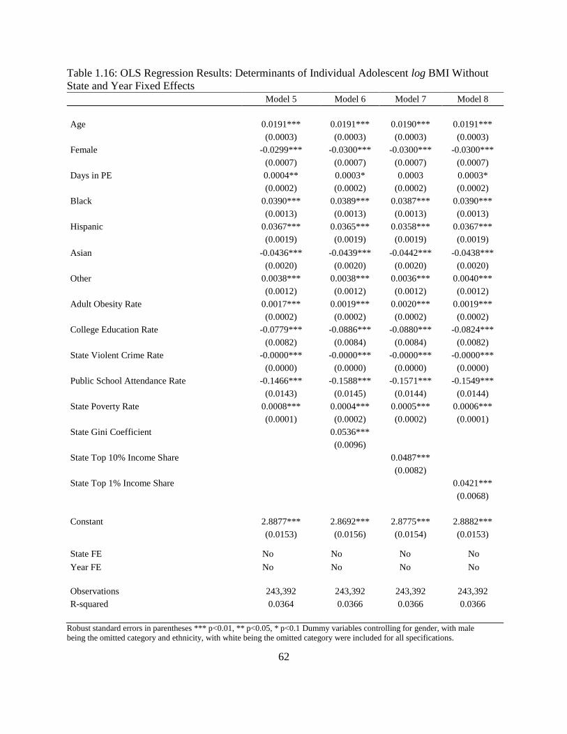
62

Table 1.16: OLS Regression Results: Determinants of Individual Adolescent log BMI Without

State and Year Fixed Effects


Age 0.0191*** 0.0191*** 0.0190*** 0.0191***

(0.0003) (0.0003) (0.0003) (0.0003)

Female -0.0299*** -0.0300*** -0.0300*** -0.0300***

(0.0007) (0.0007) (0.0007) (0.0007)

Days in PE 0.0004** 0.0003* 0.0003 0.0003*

(0.0002) (0.0002) (0.0002) (0.0002)

Black 0.0390*** 0.0389*** 0.0387*** 0.0390***

(0.0013) (0.0013) (0.0013) (0.0013)

Hispanic 0.0367*** 0.0365*** 0.0358*** 0.0367***

(0.0019) (0.0019) (0.0019) (0.0019)

Asian -0.0436*** -0.0439*** -0.0442*** -0.0438***

(0.0020) (0.0020) (0.0020) (0.0020)

Other 0.0038*** 0.0038*** 0.0036*** 0.0040***

(0.0012) (0.0012) (0.0012) (0.0012)

Adult Obesity Rate 0.0017*** 0.0019*** 0.0020*** 0.0019***

(0.0002) (0.0002) (0.0002) (0.0002)

College Education Rate -0.0779*** -0.0886*** -0.0880*** -0.0824***

(0.0082) (0.0084) (0.0084) (0.0082)

State Violent Crime Rate -0.0000*** -0.0000*** -0.0000*** -0.0000***

(0.0000) (0.0000) (0.0000) (0.0000)


(0.0143) (0.0145) (0.0144) (0.0144)


(0.0001) (0.0002) (0.0002) (0.0001)


(0.0096)


(0.0082)


(0.0068)

Constant 2.8877*** 2.8692*** 2.8775*** 2.8882***

(0.0153) (0.0156) (0.0154) (0.0153)

State FE No No No No

Year FE No No No No

Observations 243,392 243,392 243,392 243,392

R-squared 0.0364 0.0366 0.0366 0.0366


being the omitted category and ethnicity, with white being the omitted category were included for all specifications.

63

Table 1.17: OLS Regression Results: Determinants of Individual Adolescent BMI With State

and Year Fixed Effects Model 9 Model 10 Model 11 Model 12 Model 13

Age 0.4278*** 0.4282*** 0.4283*** 0.4283*** 0.4284***

(0.0073) (0.0073) (0.0073) (0.0073) (0.0073)

Female -0.7256*** -0.7254*** -0.7257*** -0.7258*** -0.7256***

(0.0171) (0.0171) (0.0171) (0.0171) (0.0171)

Days in PE 0.0032 0.0030 0.0029 0.0030 0.0029

(0.0042) (0.0042) (0.0042) (0.0042) (0.0042)

Black 1.0005*** 1.0133*** 1.0158*** 1.0119*** 1.0193***

(0.0337) (0.0339) (0.0339) (0.0339) (0.0339)

Hispanic 0.8451*** 0.8656*** 0.8696*** 0.8646*** 0.8782***

(0.0480) (0.0483) (0.0484) (0.0483) (0.0484)

Asian -0.9365*** -0.9219*** -0.9189*** -0.9227*** -0.9153***

(0.0477) (0.0478) (0.0478) (0.0478) (0.0478)

Other 0.1845*** 0.2017*** 0.2071*** 0.2008*** 0.2116***

(0.0298) (0.0302) (0.0303) (0.0302) (0.0303)

Adult Obesity Rate -0.0112 -0.0128 -0.0269** -0.0127

(0.0118) (0.0118) (0.0123) (0.0118)

College Education Rate -1.1352 -2.2428** -1.9111** -2.1859**

(0.8803) (0.9377) (0.8944) (0.9101)

State Violent Crime Rate -0.0003 -0.0000 0.0001 -0.0000

(0.0002) (0.0003) (0.0003) (0.0003)

Public School Attendance Rate -1.6950 -0.9258 -0.6682 -0.5064

(1.1709) (1.1959) (1.1991) (1.2054)

State Poverty Rate 0.0251*** 0.0266*** 0.0219** 0.0266***

(0.0094) (0.0094) (0.0094) (0.0094)

Year 2001 -0.3754*** -0.3596*** -0.3011*** -0.2710*** -0.3008***

(0.0276) (0.0410) (0.0446) (0.0454) (0.0430)

Year 2013 -0.1849*** -0.0949 0.0160 0.0083 0.0260

(0.0304) (0.1086) (0.1130) (0.1107) (0.1118)


(0.5182)


(0.6537)


(0.3434)

Constant 16.0441*** 17.7749*** 16.1548*** 16.1105*** 16.5071***

(0.1485) (1.1905) (1.2944) (1.2540) (1.2269)

State FE Yes Yes Yes Yes Yes

Year FE Yes Yes Yes Yes Yes

Observations 243,392 243,392 243,392 243,392 243,392

R-squared 0.0369 0.0370 0.0370 0.0371 0.0371


being the omitted category and ethnicity, with white being the omitted category were included for all specifications. In

Models 2 and 3, dummy variables controlling for state and years 2001, 2007, and 2013 were also included. Omitted state

Alabama, omitted year 2007. State results are reported in Appendix A.16.

64

Table 1.18: OLS Regression Results: Determinants of Individual Adolescent log BMI With State

and Year Fixed Effects Model 14 Model 15 Model 16 Model 17 Model 18

Age 0.0189*** 0.0189*** 0.0189*** 0.0189*** 0.0189***

(0.0003) (0.0003) (0.0003) (0.0003) (0.0003)

Female -0.0300*** -0.0300*** -0.0300*** -0.0300*** -0.0300***

(0.0007) (0.0007) (0.0007) (0.0007) (0.0007)

Days in PE 0.0004** 0.0003** 0.0003** 0.0004** 0.0003**

(0.0002) (0.0002) (0.0002) (0.0002) (0.0002)

Black 0.0419*** 0.0424*** 0.0425*** 0.0424*** 0.0427***

(0.0014) (0.0014) (0.0014) (0.0014) (0.0014)

Hispanic 0.0354*** 0.0363*** 0.0364*** 0.0362*** 0.0368***

(0.0019) (0.0020) (0.0020) (0.0020) (0.0020)

Asian -0.0413*** -0.0407*** -0.0406*** -0.0407*** -0.0404***

(0.0020) (0.0020) (0.0020) (0.0020) (0.0020)

Other 0.0073*** 0.0080*** 0.0082*** 0.0080*** 0.0084***

(0.0012) (0.0012) (0.0012) (0.0012) (0.0012)

Adult Obesity Rate -0.0004 -0.0004 -0.0010** -0.0004

(0.0005) (0.0005) (0.0005) (0.0005)

College Education Rate -0.0447 -0.0905** -0.0771** -0.0878**

(0.0361) (0.0385) (0.0367) (0.0373)

State Violent Crime Rate -0.0000 -0.0000 0.0000 -0.0000

(0.0000) (0.0000) (0.0000) (0.0000)

Public School Attendance Rate -0.0735 -0.0417 -0.0307 -0.0247

(0.0482) (0.0492) (0.0493) (0.0496)

State Poverty Rate 0.0011*** 0.0011*** 0.0009** 0.0011***

(0.0004) (0.0004) (0.0004) (0.0004)

Year 2001 -0.0154*** -0.0146*** -0.0122*** -0.0109*** -0.0122***

(0.0011) (0.0017) (0.0018) (0.0019) (0.0018)

Year 2013 -0.0086*** -0.0055 -0.0009 -0.0012 -0.0005

(0.0012) (0.0045) (0.0046) (0.0045) (0.0046)


(0.0212)


(0.0270)


(0.0142)

Constant 2.8118*** 2.8841*** 2.8172*** 2.8148*** 2.8321***

(0.0061) (0.0489) (0.0531) (0.0515) (0.0504)

State FE Yes Yes Yes Yes Yes

Year FE Yes Yes Yes Yes Yes

Observations 243,392 243,392 243,392 243,392 243,392

R-squared 0.0396 0.0397 0.0398 0.0398 0.0398




Alabama, omitted year 2007. State results are reported in Appendix A.7.

65

Table 1.19: Regression Results on Adolescent BMI Post Wellness Policy Implementation


Wellness Policy Index 0.0105** 0.0065* 0.0103** 0.0129***

(0.0041) (0.0042) (0.0041) (0.0042)

Age 0.4287*** 0.4283*** 0.4282*** 0.4283***

(0.0073) (0.0073) (0.0073) (0.0073)

Female -0.7260*** -0.7264*** -0.7264*** -0.7262***

(0.0171) (0.0171) (0.0171) (0.0171)

Days in PE 0.0027 0.0028 0.0030 0.0028

(0.0042) (0.0042) (0.0042) (0.0042)

Black 1.0066*** 1.0192*** 1.0101*** 1.0234***

(0.0337) (0.0338) (0.0337) (0.0338)

Hispanic 0.8584*** 0.8702*** 0.8583*** 0.8810***

(0.0484) (0.0484) (0.0484) (0.0485)

Asian -0.9257*** -0.9130*** -0.9220*** -0.9083***

(0.0477) (0.0477) (0.0477) (0.0477)

Other 0.1939*** 0.2161*** 0.2009*** 0.2210***

(0.0297) (0.0299) (0.0297) (0.0299)

Adult Obesity Rate 0.0246** 0.0140 0.0427*** 0.0183*

(0.0111) (0.0112) (0.0113) (0.0111)

College Education Rate 0.0937 -1.3039*** -0.7976** -0.8018**

(0.3456) (0.3897) (0.3587) (0.3605)

State Violent Crime Rate -0.0002 0.0002 0.0003 0.0001

(0.0002) (0.0002) (0.0002) (0.0002)


(1.0044) (1.1541) (1.1496) (1.1256)


(0.0089) (0.0090) (0.0089) (0.0089)


(0.4269)


(0.5424)


(0.3022)

Constant 24.9357*** 18.5475*** 18.8056*** 20.2043***

(1.0636) (1.3256) (1.2490) (1.1868)

Observations 243,392 243,392 243,392 243,392

R-squared 0.0366 0.0369 0.0369 0.0369

Robust standard errors in parentheses *** p<0.01, ** p<0.05, * p<0.1; Additional controls include: state dummy variables

(coefficients not reported)

66

Table 1.20: Regression Results on Adolescent log BMI Post Wellness Policy Implementation


Wellness Policy Index 0.0005*** 0.0003* 0.0005*** 0.0006***

(0.0002) (0.0002) (0.0002) (0.0002)

Age 0.0189*** 0.0189*** 0.0189*** 0.0189***

(0.0003) (0.0003) (0.0003) (0.0003)

Female -0.0300*** -0.0300*** -0.0300*** -0.0300***

(0.0007) (0.0007) (0.0007) (0.0007)

Days in PE 0.0003** 0.0003** 0.0004** 0.0003**

(0.0002) (0.0002) (0.0002) (0.0002)

Black 0.0421*** 0.0426*** 0.0423*** 0.0428***

(0.0014) (0.0014) (0.0014) (0.0014)

Hispanic 0.0359*** 0.0364*** 0.0359*** 0.0369***

(0.0020) (0.0020) (0.0020) (0.0020)

Asian -0.0409*** -0.0404*** -0.0408*** -0.0402***

(0.0020) (0.0020) (0.0020) (0.0020)

Other 0.0076*** 0.0085*** 0.0079*** 0.0087***

(0.0012) (0.0012) (0.0012) (0.0012)

Adult Obesity Rate 0.0010** 0.0006 0.0018*** 0.0008*

(0.0005) (0.0005) (0.0005) (0.0005)

College Education Rate -0.0048 -0.0631*** -0.0420*** -0.0421***

(0.0142) (0.0159) (0.0147) (0.0148)

State Violent Crime Rate -0.0000 0.0000 0.0000 0.0000

(0.0000) (0.0000) (0.0000) (0.0000)


(0.0414) (0.0476) (0.0473) (0.0465)


(0.0004) (0.0004) (0.0004) (0.0004)


(0.0174)


(0.0223)


(0.0124)

Constant 3.1857*** 2.9191*** 2.9296*** 2.9885***

(0.0437) (0.0544) (0.0513) (0.0489)

Observations 243,392 243,392 243,392 243,392

R-squared 0.0393 0.0396 0.0397 0.0396

Robust standard errors in parentheses *** p<0.01, ** p<0.05, * p<0.1; Additional controls include: state dummy variables


67

Chapter 11: Dominance Analysis

Dominance analysis is a statistical technique used to determine the relative importance of

an individual variable based on the contribution of all pairs of explanatory variables to the

overall variance of regression models containing all possible subsets of explanatory variables

(Azen and Budescu, 2003). It allows each variable to be ranked from most important to least

important according to how much of the additional overall explained variance of the model is

explained by the variable (Grömping, 2007; Luchman, 2015). Azen and Budescu (2013) define

three levels of dominance: complete, conditional, and general. Complete dominance exists when

an explanatory variable has a greater contribution to the explained variance of the model than the

dominated variable in all possible subset regressions. Conditional dominance exists when the

average additional contribution to the explained variance of the model is greater for one

explanatory variable compared to the dominated variable across all possible subset regressions.

Finally, general dominance exists when the average additional contribution to the explained

variance of the model is greater for one explanatory variable compared to the dominated variable

across subset regressions of the same size.

Principal component analysis resulted in four factors that were used to generate the

wellness policy index score for each state in the SHPPS survey years 2000, 2006, and 2012 (see

Table 1.7). These four factors were: 1) policy that met national standards, 2) policy that met a

state requirement, 3) policy that met health screening criteria, and 4) policy that met state

recommendations. Of particular interest in this research is the relative importance of each of

68

these factors in the regression analysis of the wellness policy effect on adolescent BMI trends.

Dominance analysis was performed in STATA (version 12) using the “domin” command.

Results of the dominance analysis are reported in Table 1.21.

Table 1.21: Dominance Analysis Results

Factor 2 completely dominates Factor 1

Factor 3 completely dominates Factor 1

Factor 2 conditionally dominates Factor 4

Factor 4 generally dominates Factor 1



The dominance analysis ranking of the factors and their associated SHPPS survey variables are

given in Table 1.22. 1) policy that met state requirements, 2) policy that met health screening

criteria, 3) policy that met state recommendations, and 4) policy that met national standards.

Interestingly, the factor ranked as most important contained survey items related to state

wellness policy components required by the 2004 CRNA federal mandate (see Table 1.1) while

the least impactful factor was related to policies that met national standards. Furthermore, health

screening also appears to be an important component of the wellness policy implementation.

Perhaps identifying students who are at risk of being overweight or obese through routine school

health screenings and following through with family involvement by reporting the screening

information, school health officials and staff might help slow the current obesity trend among

adolescents.

69

Table 1.22: Dominance Analysis Factor Ranking

#1: Policy that met state requirements

Health education required

Food service education required

Physical education required

Family/Community involvement required

#2: Policy that met health screening criteria

Student health history

General health screening

PE exempt screening

#3: Policy that met state recommendations

Onsite fast food restrictions

School wellness policy coordinator

#4 Policy that met national standards

National health education standards

USDA nutrition standards

Physical education activity required

70

Chapter 12: Discussion

12.1 Conclusions

The prevalence of adolescent BMI is currently above the current health policy goal of

14.5% set forth in Healthy People 2020. In this research, I examined whether varying degrees of

state wellness policy execution, as required by the Child Nutrition and WIC Reauthorization Act

of 2004 explained the variation in the prevalence of adolescent obesity as measured by BMI. The

results showed that prior to the federal policy being passed in 2006, states were already reacting

to the obesity crisis and beginning to formulate their own wellness policy strategies.

Regression results indicated that there was little effect on the increasing BMI trends. This

result is not surprising; weight loss and its associated lower BMI measure, happens over time as

diet and physical activity changes occur. The fuller effects of each state’s health education,

nutrition, and physical activity wellness policy components would be expected to be seen in

subsequent years following implementation. Even so, the disparity in effectiveness of the

wellness policy implementation among states was evident. This is a direct reflection of the

ambiguity of the policy mandate itself; states were tasked with having a written policy in place

that would address health education, physical activity and education, nutrition, family and

community involvement, and faculty/staff health promotion however, there were no stated

standards or accountability mechanisms given in the mandate.

71

States had broad latitude in their interpretation and thus the level of implementation of the

wellness policies; it is not unexpected that some states experienced better adolescent BMI

outcomes than others as a result of these inconsistencies.

Understanding the determinants of adolescent obesity and how to effect change in the

rising trend is a national concern. Obese adolescents are at significant risk of becoming obese

adults and previous research has already shown the high economic costs associated with adult

obesity and its comorbidities. Of great concern is that obese children and adolescents are now

also being diagnosed with obesity-related diseases such as type-2 diabetes, high blood pressure,

and cardiovascular disease that were previously diagnosed in adults. Policies implemented in

school, where adolescents consume a considerable portion of their daily calories and participate

in physical activity, can help to build healthy habits that have the potential to lower the

probability of an adolescent becoming an obese adult. Over time, a healthier adult population

may result in lower economic costs associated with medical care and lost productivity.

12.2 Study Limitations

One of the disadvantages in using the YRBSS is that the CDC does not release school-

level identifiers so I am unable to distinguish private from public school students. Since public

schools are legally bound to comply with federal mandates whereas private schools are not,

results obtained may be biased. Although the state requirements for public schools may set a

standard that is adopted by private schools, the impact of state regulations is likely to be less for

private school students than public school students.

72

Since the models were estimated with a pooled sample of public and private school students, the

estimates will likely underestimate the impact of state regulations on public school students.

An additional limitation of this data is that weight and height are self-reported in the

YRBSS and are therefore likely reported with error. Although other studies have shown that high

school students tend to report height and weight that understates the prevalence of obesity, future

research should include observed height and weight data in order to corroborate the results of

this study.

Finally, a drawback of this research is that I only observe the state of residence for each

student. Therefore, I was only able to use state-level variables in the analysis. Future research

should observations at an individual level that can be matched with corresponding county or

school data.

12.3 Future Research

Future research in adolescent obesity should include investigation of peer effects. These

studies could examine how and to what extent weight status of younger students is affected by

their older peers. Similar analysis of same grade peers should also be performed. An

understanding of the existence of such peer effects would allow emphasis to be placed on the

interventions most likely to affect obesity trends.

Continued research in adolescent obesity should include analysis of specific interventions

related to the five general components of the CRNA. Data at the individual student’s school level

will help to overcome the bias present in research that utilizes aggregate data. Given the

appropriate level of data, this research could be extended to the individual student’s county or

school. The use of micro-level data would enhance the capability to study not only the effect of a

73

school’s wellness policy index overall on adolescent obesity trends, but would also allow for

analysis of the interaction of the various policy components.

Finally, through use of a suitable instrument for the wellness policy index, potential bias

that may exist due to schools, school districts, and state education agencies choosing to

implement stricter wellness policies due to existing adolescent obesity trends can be addressed.

74

References Cited

Albrecht, S.S., Gordon-Larsen, P., 2013. Ethnic Differences in Body Mass Index Trajectories

from Adolescence to Adulthood: A Focus on Hispanic and Asian Subgroups in the

United States. PLoS ONE 8, e72983. doi:10.1371/journal.pone.0072983

Anderson, P.M., Butcher, K.F., 2006. Childhood obesity: trends and potential causes. Future

Child. 16, 19–45.

Anderson, P.M., Butcher, K.F., Levine, P.B., 2003. Maternal employment and overweight

children. J. Health Econ. 22, 477–504.

Anderson, S.E., Cohen, P., Naumova, E.N., Must, A., Association of depression and anxiety

disorders with weight change in a prospective community-based study of children

followed up into adulthood. Archives of pediatrics & adolescent medicine. 285-291.

Azen, R., Budescu, D.V., 2003. The dominance analysis approach for comparing predictors in

multiple regression. Psychol. Methods 8, 129–148. doi:10.1037/1082-989X.8.2.129

Becker, G.S., Murphy, K.M., 1988. A theory of rational addiction. J. Polit. Econ. 675–700.

Bethell, C., Simpson, L., Stumbo, S., Carle, A.C., Gombojav, N., 2010. National, state, and local

disparities in childhood obesity. Health Aff. (Millwood) 29, 347–356.

Bhattacharya, J., Sood, N., 2007. Health insurance and the obesity externality. Adv. Health Econ.

Health Serv. Res. 17, 279–318.

Birch, L.L., Deysher, M., 1985. Conditioned and unconditioned caloric compensation: evidence

for self-regulation of food intake in young children. Learn. Motiv. 16, 341–355.

Birch, L.L., Fisher, J.O., 1998. Development of eating behaviors among children and

adolescents. Pediatrics 101, 539–549.

Biro, F.M., Wien, M., 2010. Childhood obesity and adult morbidities. Am. J. Clin. Nutr. 91,

1499S–1505S.

Brener, N.D., McManus, T., Galuska, D.A., Lowry, R., Wechsler, H., 2003. Reliability and

validity of self-reported height and weight among high school students. J. Adolesc.

Health 32, 281–287.

75

Burkhauser, R.V., Cawley, J., 2004. Obesity, disability, and movement onto the disability

insurance rolls. Mich. Retire. Res. Cent. Res. Pap. No WP 89.

Caprio, S., Daniels, S.R., Drewnowski, A., Kaufman, F.R., Palinkas, L.A., Rosenbloom, A.L.,

Schwimmer, J.B., 2008. Influence of Race, Ethnicity, and Culture on Childhood Obesity:

Implications for Prevention and Treatment A consensus statement of Shaping America’s

Health and the Obesity Society. Diabetes Care 31, 2211–2221. doi:10.2337/dc08-9024

Cawley, J., 2010. 3. The economics of childhood obesity policy. Obes. Bus. Public Policy 27.

Centers for Disease Control and Prevention, 2011. About BMI for children and teens. 2011.

Updat. June 2Available Httpwww Cdc

Govhealthyweightassessingbmichildrensbmiaboutchildrensbmi Html.

Chou, S.-Y., Grossman, M., Saffer, H., 2004. An economic analysis of adult obesity: results

from the Behavioral Risk Factor Surveillance System. J. Health Econ. 23, 565–587.

Chriqui, J.F., Schneider, L., Kristen, I., Grourdet, C., Bruursema, A., 2010. Bridging the Gap

(BTG) Program: School District Wellness Policy Coding Tool, v. 2. Chic. IL Univ. Ill.

Chic.

Coffield, J.E., Metos, J.M., Utz, R.L., Waitzman, N.J., 2011. A multivariate analysis of federally

mandated school wellness policies on adolescent obesity. J. Adolesc. Health 49, 363–370.

Coneus, K., Spiess, C.K., 2012. The intergenerational transmission of health in early

childhood—Evidence from the German Socio-Economic Panel Study. Econ. Hum. Biol.

10, 89–97. doi:10.1016/j.ehb.2011.03.002

Council on Communications and Media, 2011. Children, Adolescents, Obesity, and the Media.

PEDIATRICS 128, 201–208. doi:10.1542/peds.2011-1066

Cutler, D., Glaeser, E., Shapiro, J., 2003. Why have Americans become more obese? National

Bureau of Economic Research.

Dietz, W.H., 1998. Health consequences of obesity in youth: childhood predictors of adult

disease. Pediatrics 101, 518–525.

Ding, W., Lehrer, S.F., Rosenquist, J.N., Audrain-McGovern, J., 2009. The impact of poor health

on academic performance: New evidence using genetic markers. J. Health Econ. 28, 578–

597.

Egan, T., 2002. In bid to improve nutrition, schools expel soda and chips. N. Y. Times 20, 2002.

Filmer, D., Pritchett, L.H., 2001. Estimating wealth effects without expenditure Data—Or tears:

An application to educational enrollments in states of india*. Demography 38, 115–132.

76

Finkelstein, E.A., Ruhm, C.J., Kosa, K.M., 2005. Economic causes and consequences of obesity.

Annu Rev Public Health 26, 239–257.

Finkelstein, E.A., Trogdon, J.G., Cohen, J.W., Dietz, W., 2009. Annual medical spending

attributable to obesity: payer-and service-specific estimates. Health Aff. (Millwood) 28,

w822–w831.

Frank, M.W., 2013. U.S. State-Level Income Inequality Data.

Freedman, D.S., Khan, L.K., Serdula, M.K., Ogden, C.L., Dietz, W.H., 2006. Racial and ethnic

differences in secular trends for childhood BMI, weight, and height. Obes. Silver Spring

Md 14, 301–308. doi:10.1038/oby.2006.39

Frezza, E.E., Wachtel, M.S., Ewing, B.T., 2006. The impact of morbid obesity on the state

economy: an initial evaluation. Surg. Obes. Relat. Dis. 2, 504–508.

Gleason, P., Suitor, C., 2001. Food for Thought: Children’s Diets in the 1990s. Policy Brief.

Goldberg, M.E., Gorn, G.J., Gibson, W., 1978. TV messages for snack and breakfast foods: do

they influence children’s preferences? J. Consum. Res. 73–81.

Goodman, E., Whitaker, R.C., 2002. A prospective study of the role of depression in the

development and persistence of adolescent obesity. Pediatrics. 497-504.

Grömping, U., 2007. Estimators of Relative Importance in Linear Regression Based on Variance

Decomposition. Am. Stat. 61, 139–147. doi:10.1198/000313007X188252

Grossman, M., 1972. On the concept of health capital and the demand for health. J. Polit. Econ.

223–255.

Haines, J., Neumark-Sztainer, D., Hannan, P., Robinson-O’Brien, R., 2008. Child versus Parent

Report of Parental Influences on Children’s Weight-related Attitudes and Behaviors. J.

Pediatr. Psychol. 33, 783–788. doi:10.1093/jpepsy/jsn016

Harris, J.L., Bargh, J.A., Brownell, K.D., 2009. Priming effects of television food advertising on

eating behavior. Health Psychol. 28, 404.

Harris, J.M., Shiptsova, R., others, 2007. Consumer demand for convenience foods:

Demographics and expenditures. J. Food Distrib. Res. 38, 22.

Hendrikse, J.J., Cachia, R.L., Kothe, E.J., McPhie, S., Skouteris, H., Hayden, M.J., 2015.

Attentional biases for food cues in overweight and individuals with obesity: a systematic

review of the literature: Attentional biases and obesity. Obes. Rev. 16, 424–432.

doi:10.1111/obr.12265

77

Hill, J.O., Trowbridge, F.L., 1998. Childhood obesity: future directions and research priorities.

Pediatrics 101, 570–574.

Hines, R., Dobrzynski, L., Huang, D., Pearcy, J., Rose, C., Rosendorf, K., Talih, M., 2011.

Healthy People 2010 Final Review [WWW Document]. URL

http://www.cdc.gov/nchs/healthy_people/hp2010/hp2010_final_review.htm (accessed

10.10.15).

Hotelling, H., 1933. Analysis of a complex of statistical variables into principal components. J.

Educ. Psychol. 24, 417–441. doi:10.1037/h0071325

Institute of Medicine (U.S.), Glickman, D. (Eds.), 2012. Accelerating progress in obesity

prevention: solving the weight of the nation. National Academies Press, Washington, DC.

Jacobson, L., 2000. The family as producer of health—an extended Grossman model. J. Health

Econ. 19, 611–637.

Joint Research Centre-European Commission, J.R.C.-E., others, 2008. Handbook on constructing

composite indicators: Methodology and User guide. OECD publishing.

Jolliffe, I.T., 2002. Principal component analysis, 2nd ed. ed, Springer series in statistics.

Springer, New York.

Just, D.R., Mancino, L., Wansink, B., 2007. Could Behavioral Economics Help Improve Diet

Quality for Nutrition Assistance Program Participants? SSRN Electron. J.

doi:10.2139/ssrn.1084548

Kaiser, H.F., 1960. The application of electronic computers to factor analysis. Educ. Psychol.

Meas.

Kann, L., Brener, N.D., Wechsler, H., 2007. Overview and summary: School health policies and

programs study 2006. J. Sch. Health 77, 385–397.

Katz, D.L., 2009. School-based interventions for health promotion and weight control: not just

waiting on the world to change. Annu. Rev. Public Health 30, 253–272.

Kohl-III, H.W., Hobbs, K.E., 1998. Development of physical activity behaviors among children

and adolescents. Pediatrics 101.

Kolenikov, S., Angeles, G., 2009. Socioeconomic status measurement with discrete proxy

variables: Is principal component analysis a reliable answer? Rev. Income Wealth 55,

128–165.

78

Kubik, M.Y., Lytle, L.A., Story, M., 2005. Schoolwide food practices are associated with body

mass index in middle school students. Arch. Pediatr. Adolesc. Med. 159, 1111–1114.

Lakdawalla, D., Philipson, T., 2002. The growth of obesity and technological change: a

theoretical and empirical examination. National Bureau of Economic Research.

Lambert, L.G., Monroe, A., Wolff, L., 2010. Mississippi elementary school teachers’

perspectives on providing nutrition competencies under the framework of their school

wellness policy. J. Nutr. Educ. Behav. 42, 271–276.

Lightwood, J., Bibbins-Domingo, K., Coxson, P., Wang, Y.C., Williams, L., Goldman, L., 2009.

Forecasting the future economic burden of current adolescent overweight: an estimate of

the coronary heart disease policy model. Am. J. Public Health 99, 2230.

Longley, C.H., Sneed, J., 2009. Effects of federal legislation on wellness policy formation in

school districts in the United States. J. Am. Diet. Assoc. 109, 95–101.

Luchman, J.N., 2015. Determining Subgroup Difference Importance with Complex Survey

Designs. Surv. Pract. 8.

MacCallum, R.C., Widaman, K.F., Zhang, S., Hong, S., 1999. Sample size in factor analysis.

Psychol. Methods 4, 84.

Metos, J., Nanney, M.S., 2007. The strength of school wellness policies: one state’s experience.

J. Sch. Health 77, 367–372.

Millimet, D.L., Tchernis, R., Husain, M., 2010. School nutrition programs and the incidence of

childhood obesity. J. Hum. Resour. 45, 640–654.

Moag-Stahlberg, A., Howley, N., Luscri, L., 2008. A national snapshot of local school wellness

policies. J. Sch. Health 78, 562–568.

National Survey of Children’s Health, n.d.

Offer, A., Pechey, R., Ulijaszek, S.J. (Eds.), 2012. Insecurity, inequality, and obesity in affluent

societies, Proceedings of the British Academy. Oxford University Press, Oxford.

Ogden, C.L., Carroll, M.D., Curtin, L.R., Lamb, M.M., Flegal, K.M., 2010. Prevalence of high

body mass index in US children and adolescents, 2007-2008. Jama 303, 242–249.

Organization for Economic Cooperation and Development, 2008. Society at a Glance 2009:

OECD Social Indicators. OECD Publishing.

79

Parikka, S., Mäki, P., Levälahti, E., Lehtinen-Jacks, S., Martelin, T., Laatikainen, T., 2015.

Associations between parental BMI, socioeconomic factors, family structure and

overweight in Finnish children: a path model approach. BMC Public Health 15, 271.

doi:10.1186/s12889-015-1548-1

Philipson, T.J., Posner, R.A., 1999. The long-run growth in obesity as a function of technological

change. National bureau of economic research.

Probart, C., McDonnell, E.T., Jomaa, L., Fekete, V., 2010. Lessons from Pennsylvania’s mixed

response to federal school wellness law. Health Aff. (Millwood) 29, 447–453.

Ravelli, A., Roseboom, T., Painter, R., de Rooij, S., 2007. The Dutch Famine Birth Cohort

Study: Hungerwinter Study.

Reilly, J.J., Kelly, J., 2011. Long-term impact of overweight and obesity in childhood and

adolescence on morbidity and premature mortality in adulthood: systematic review. Int. J.

Obes. 35, 891–898.

Ricci, J.A., Chee, E., 2005. Lost productive time associated with excess weight in the US

workforce. J. Occup. Environ. Med. 47, 1227–1234.

Riis, J., Grason, H., Strobino, D., Ahmed, S., Minkovitz, C., 2012. State school policies and

youth obesity. Matern. Child Health J. 16, 111–118.

Rowlingson, K., 2011. Does income inequality cause health and social problems? (Report).

Joseph Rowntree Foundation, London.

Sabia, J.J., 2007. The effect of body weight on adolescent academic performance. South. Econ. J.

871–900.

Schanzenbach, D.W., 2009. Do School Lunches Contribute to Childhood Obesity? J. Hum.

Resour. 44, 684–709. doi:10.3368/jhr.44.3.684

Schwartz, M.B., Puhl, R., 2003. Childhood obesity: a societal problem to solve. Obes. Rev. 4,

57–71. doi:10.1046/j.1467-789X.2003.00093.x

Serdula, M.K., Ivery, D., Coates, R.J., Freedman, D.S., Williamson, D.F., Byers, T., 1993. Do

Obese Children Become Obese Adults? A Review of the Literature. Prev. Med. 22, 167–

177. doi:10.1006/pmed.1993.1014

Simon, H.A., 1955. A behavioral model of rational choice. Q. J. Econ. 99–118.

Snyder, T., Dillow, S., 2012. Average daily attendance as a percentage of total enrollment,

school day length, and school year length in public schools, by school level and state:

2003-04 and 2007-08.

80

Story, M., Nanney, M.S., Schwartz, M.B., 2009. Schools and Obesity Prevention: Creating

School Environments and Policies to Promote Healthy Eating and Physical Activity.

Milbank Q. 87, 71–100. doi:10.1111/j.1468-0009.2009.00548.x

Strauss, R.S., Pollack, H.A., 2003. Social Marginalization of Overweight Children. Arch.

Pediatr. Adolesc. Med. 157, 746. doi:10.1001/archpedi.157.8.746

Svensson, V., Jacobsson, J.A., Fredriksson, R., Danielsson, P., Sobko, T., Schiöth, H.B., Marcus,

C., 2011. Associations between severity of obesity in childhood and adolescence, obesity

onset and parental BMI: a longitudinal cohort study. Int. J. Obes. 35, 46–52.

doi:10.1038/ijo.2010.189

Trasande, L., Chatterjee, S., 2009. The Impact of Obesity on Health Service Utilization and

Costs in Childhood. Obesity 17, 1749–1754. doi:10.1038/oby.2009.67

US Department of Health and Human Services, 2012. Healthy People 2020. Washington, DC.

Wang, Y., Zhang, Q., 2006. Are American children and adolescents of low socioeconomic status

at increased risk of obesity? Changes in the association between overweight and family

income between 1971 and 2002. Am. J. Clin. Nutr. 84, 707–716.

Wharton, C.M., Long, M., Schwartz, M.B., 2008. Changing Nutrition Standards in Schools: The

Emerging Impact on School Revenue. J. Sch. Health 78, 245–251. doi:10.1111/j.1746-

1561.2008.00296.x

Whitaker, R.C., Wright, J.A., Pepe, M.S., Seidel, K.D., Dietz, W.H., 1997. Predicting Obesity in

Young Adulthood from Childhood and Parental Obesity. N. Engl. J. Med. 337, 869–873.

doi:10.1056/NEJM199709253371301

Wilkinson, R.G., Pickett, K.E., 2009. Income Inequality and Social Dysfunction. Annu. Rev.

Sociol. 35, 493–511. doi:10.1146/annurev-soc-070308-115926

Wilkinson, R., Pickett, K., 2009. The spirit level: Why greater equality makes societies stronger.

Bloomsbury Publishing USA.

Zimmerman, F.J., 2011. Using Marketing Muscle to Sell Fat: The Rise of Obesity in the Modern

Economy. Annu. Rev. Public Health 32, 285–306. doi:10.1146/annurev-publhealth-

090810-182502

81

Appendices

82

Appendix A: Additional Tables

Table A.1 Correlation Matrix of Individual-Level Demographic Explanatory Variables Used in Regression Analysis

BMI log BMI Age Female Black Hispanic Asian Other daysPE

BMI 1

log BMI 0.993 1

(0.000)

Age 0.125 0.134 1

(0.000) (0.000)

Female -0.0889 -0.0898 -0.0380 1

(0.000) (0.000) (0.000)

Black 0.0728 0.0741 0.00218 0.00980 1

(0.000) (0.000) (0.282) (0.000)

Hispanic 0.0352 0.0363 0.0102 -0.000295 -0.0776 1

(0.000) (0.000) (0.000) (0.884) (0.000)

Asian -0.0508 -0.0536 -0.00257 -0.00546 -0.0681 -0.0373 1

(0.000) (0.000) (0.205) (0.007) (0.000) (0.000)

Other -0.0224 -0.0252 -0.0311 -0.00428 -0.356 -0.195 -0.171 1

(0.000) (0.000) (0.000) (0.035) (0.000) (0.000) (0.000)

daysPE -0.0140 -0.0126 -0.189 -0.0968 0.00699 0.0225 0.00844 -0.0441 1

(0.000) (0.000) (0.000) (0.000) (0.001) (0.000) (0.000) (0.000) p-values in parentheses

83

Table A.2: Correlation Matrix of State-Level Explanatory Variables Used In Regression Analysis

BMI log BMI

Wellness

Policy

Index

State

Adult

Obesity

Rate

State

College

Education

Rate

State

Poverty

Rate

State

Violent

Crime

Rate

State Gini

Coefficient

State Top

10%

Income

Share

State Top

1%

Income

Share

State Public

School

Attendance

Rate

BMI 1

log BMI 0.9930 1

(0.000)

Wellness Policy Index 0.0231 0.0161 1

(0.019) (0.007)

State Adult Obesity

Rate

0.0417

(0.000)

0.0386

(0.000)

0.1590

(0.000)

1

State College

Education Rate

-0.0224

(0.000)

-0.0242

(0.000)

0.156

(0.000)

0.0522

(0.000)

1

State Poverty Rate 0.0363 0.0333 -0.0205 0.4490 -0.3030 1

(0.000) (0.000) (0.000) (0.000) (0.000)

State Violent Crime

Rate

0.0175

(0.000)

0.0166

(0.000)

-0.0955

(0.000)

0.2800

(0.000)

-0.1780

(0.000)

0.2870

(0.000)

1

State Gini Coefficient 0.0133 0.0124 -0.3260 -0.0150 0.0827 0.3380 0.1840 1

(0.000) (0.000) (0.000) (0.000) (0.000) (0.000) (0.000)

State Top 10% Income

Share

0.0138

(0.000)

0.0137

(0.000)

-0.3900

(0.000)

-0.0926

(0.000)

0.0922

(0.000)

0.2560

(0.000)

0.1680

(0.000)

0.8800

(0.000)

1

State Top 1% Income

Share

0.0123

(0.000)

0.0125

(0.000)

-0.4400

(0.000)

-0.0770

(0.000)

-0.0111

(0.000)

0.1460

(0.000)

0.1320

(0.000)

0.8850

(0.000)

0.8860

(0.000)

1

State Public School

Attendance Rate

-0.0026

(0.173)

-0.0025

(0.185)

-0.0747

(0.000)

-0.0862

(0.000)

-0.5400

(0.000)

0.2530

(0.000)

-0.2100

(0.000)

0.0631

(0.000)

0.0300

(0.000)

0.0621

(0.000)

1

p-values in parentheses

84

Table A.3: Mean BMI by State and YRBSS Survey Year

Mean (all years) 2001 2007 2013

Alabama 23.24 22.94 23.66

Arizona 22.90 22.78 22.71

Arkansas 23.18 22.93 23.09 23.56

Connecticut 22.86 23.07 22.77

Delaware 23.12 22.75 23.20 23.30

Florida 22.73 22.66 22.81 22.77

Georgia 23.21 23.47 23.14

Idaho 22.51 22.11 22.76 22.65

Indiana 23.24 23.53

Kansas 22.90 22.93 22.91

Kentucky 23.37 23.33 23.42

Maine 22.89 22.70 22.97 22.80

Maryland 22.64 23.12 22.59

Massachusetts 22.72 22.70 22.79 22.65

Michigan 22.85 22.64 23.17 22.85

Mississippi 23.43 23.29 23.96 22.91

Missouri 23.05 22.92 23.22 23.13

Montana 22.42 22.16 22.48 22.52

New Hampshire 22.94 23.05 22.89

New Jersey 22.71 22.59 22.56

New Mexico 22.53 22.48 22.60

New York 22.92 23.11 22.71

North Carolina 22.97 22.79 23.08 22.82

North Dakota 22.74 22.45 22.77 23.18

Ohio 23.05 23.12 23.15

Oklahoma 23.21 23.48 22.68

Rhode Island 22.87 22.50 22.96 22.86

South Carolina 23.04 23.30 23.06

South Dakota 22.67 22.46 22.74 22.82

Tennessee 23.54 23.80 23.76

Texas 23.45 23.38 23.54 23.51

Utah 21.85 21.67 22.04 21.80

Vermont 22.65 22.47 22.92 22.76

West Virginia 23.15 23.30 23.12

Wisconsin 22.86 22.84 23.02 22.91

Wyoming 22.34 21.99 22.40 22.59

85

Table A.4: Mean Adolescent BMI by Year

Mean

Standard


2001 22.67 4.07 13.06 39.99

2007 23.04 4.27 13.02 39.99

2013 22.76 4.30 12.91 39.99

Table A.5: Mean Adolescent BMI by Region and YRBSS Survey Year

Mean (all years) 2001 2007 2013

New England

Mean 22.76

(4.11)

22.56

(3.91)

22.94

(4.11)

22.77

(4.26)

East North Central

Mean 22.94

(4.20)

22.72

(4.02)

23.20

(4.25)

22.92

(4.30)

West North Central

Mean

22.83

(4.13)

22.62

(4.00)

22.90

(4.11)

23.02

(4.39)

South Atlantic

Mean

22.86

(4.28)

22.72

(4.13)

23.13

(4.34)

22.68

(4.24)

East South Central

Mean

23.40

(4.62)

23.12

(4.45)

23.59

(4.65)

23.46

(4.87)

West South Central

Mean

23.34

(4.52)

23.29

(4.48)

23.42

(4.56)

23.33

(4.63)

Mountain

Mean

22.43

(4.06)

22.03

(3.62)

22.47

(4.11)

22.50

(4.16)

Pacific

Mean 22.89 22.59 23.11 22.69

(4.22)

(3.98)

(4.20)

(4.29)

Standard deviations in parentheses.

86

Table A.6: Mean Wellness Policy Index by State and SHPPS Survey Year

SHPPS Survey Year

Mean (all years) 2000 2006 2012

Year by Year

Trend

Alabama 8.97 9.57 12.26 13.93

Arizona 7.99 4.25 9.65 12.66

Arkansas 8.10 11.42 7.08 11.79

Connecticut 14.48 13.04 14.21 16.52

Delaware 8.55 7.52 10.03 15.88

Florida 8.94 11.63 6.69 9.31

Georgia 8.36 5.02 9.86 10.24

Idaho 10.25 7.94 11.70 12.20

Indiana 12.06 12.92 11.65 12.02

Kansas 14.23 10.98 16.03 11.93

Kentucky 14.02 14.44 15.05 8.36

Maine 13.11 9.53 12.26 16.72

Maryland 13.50 18.60 13.37 13.37

Massachusetts 11.08 13.22 13.48 12.18

Michigan 10.13 10.12 11.18 13.63

Mississippi 10.58 4.83 15.60 17.11

Missouri 11.32 11.43 16.67 11.86

Montana 11.24 12.26 13.79 10.87

New Hampshire 7.11 5.02 8.64 6.13

New Jersey 10.12 6.45 13.10 11.49

New Mexico 15.54 8.84 19.22 13.37

New York 10.84 13.56 12.37 5.23

North Carolina 16.31 15.05 17.24 16.72

North Dakota 11.74 11.08 14.93 15.30

Ohio 7.37 9.90 8.49 10.20

Oklahoma 10.60 7.24 12.44 11.31

Rhode Island 9.94 8.36 11.70 6.69

South Carolina 9.44 17.83 14.21 17.83

South Dakota 10.77 10.70 15.71 5.01

Tennessee 11.14 11.14 9.47 16.97

Texas 8.93 9.72 6.37 15.07

Utah 11.02 12.82 13.37 10.03

Vermont 11.65 12.54 10.03 15.05

West Virginia 13.18 17.55 13.37 15.78

Wisconsin 13.58 12.54 16.30 14.97

Wyoming 6.87 9.19 8.36 1.67

87

Table A.7: Mean Prevalence of Adult Obesity by State


Alabama 35.48 0.0105 35.47-35.49

Arizona 36.75 0.0123 36.73-36.77

Arkansas 35.14 0.0095 35.12-35.16

Connecticut 37.31 0.0089 37.29-37.33

Delaware 36.04 0.0089 36.01-36.06

Florida 36.77 0.0044 36.75-36.79

Georgia 35.96 0.0077 35.94-35.98

Idaho 36.24 0.0205 36.22-36.25

Indiana 35.28 0.0045 35.27-35.29

Kansas 35.73 0.0006 35.72-35.75

Kentucky 36.99 0.0089 36.95-37.03

Maine 37.06 0.0069 37.05-37.07

Maryland 35.95 0.0118 35.95-35.95

Massachusetts 35.19 0.0116 35.17-35.21

Michigan 35.08 0.0083 35.07-35.10

Mississippi 35.13 0.0083 35.10-35.15

Missouri 35.09 0.0135 35.07-35.11

Montana 36.96 0.0073 36.95-36.98

New Hampshire 36.14 0.0040 36.13-36.13

New Jersey 36.77 0.0102 36.75-36.80

New Mexico 36.65 0.0089 36.63-36.66

New York 36.01 0.0126 36.00-36.02

North Carolina 35.65 0.0067 35.63-35.67

North Dakota 37.55 0.0086 37.53-37.57

Ohio 35.63 0.0051 35.60-35.65

Oklahoma 35.74 0.0056 35.73-35.76

Rhode Island 37.44 0.0094 37.42-37.46

South Carolina 35.19 0.0091 35.18-35.20

South Dakota 37.17 0.0055 37.16-37.18

Tennessee 35.98 0.0065 35.96-36.00

Texas 35.80 0.0129 35.78-35.81

Utah 34.58 0.0089 34.57-34.59

Vermont 35.50 0.0085 35.49-35.51

West Virginia 35.39 0.0105 35.36-35.41

Wisconsin 36.62 0.0123 36.60-36.63

Wyoming 36.50 0.0095 36.48-36.51

88

Table A.8: Mean College Education Rate by State


Alabama 0.1621 0.0004 0.1613-0.1628

Arizona 0.1900 0.0003 0.1894-0.1906

Arkansas 0.1409 0.0004 0.1402-0.1416

Connecticut 0.2791 0.0005 0.2782-0.2800

Delaware 0.2050 0.0004 0.2042-0.2057

Florida 0.2007 0.0002 0.2003-0.2011

Georgia 0.1969 0.0004 0.1961-0.1976

Idaho 0.1752 0.0004 0.1744-0.1761

Indiana 0.1693 0.0004 0.1685-0.1701

Kansas 0.2336 0.0006 0.2325-0.2347

Kentucky 0.1500 0.0003 0.1494-0.1505

Maine 0.2326 0.0003 0.2321-0.2332

Maryland 0.3208 0.0001 0.3206-0.3210

Massachusetts 0.2672 0.0004 0.2665-0.2680

Michigan 0.1845 0.0003 0.1839-0.1850

Mississippi 0.1435 0.0003 0.1430-0.1441

Missouri 0.1795 0.0004 0.1787-0.1803

Montana 0.2028 0.0003 0.2022-0.2034

New Hampshire 0.2622 0.0006 0.2610-0.2635

New Jersey 0.2769 0.0007 0.2755-0.2783

New Mexico 0.1806 0.0001 0.1804-0.1808

New York 0.2510 0.0003 0.2505-0.2515

North Carolina 0.1844 0.0003 0.1838-0.1850

North Dakota 0.1982 0.0005 0.1972-0.1992

Ohio 0.1859 0.0004 0.1850-0.1867

Oklahoma 0.1729 0.0004 0.1721-0.1737

Rhode Island 0.2432 0.0005 0.2422-0.2441

South Carolina 0.1709 0.0004 0.1701-0.1717

South Dakota 0.1783 0.0004 0.1776-0.1790

Tennessee 0.1815 0.0004 0.1807-0.1823

Texas 0.1829 0.0003 0.1823-0.1835

Utah 0.1907 0.0005 0.1898-0.1916

Vermont 0.2678 0.0002 0.2674-0.2683

West Virginia 0.1423 0.0004 0.1415-0.1431

Wisconsin 0.1989 0.0004 0.1981-0.1997

Wyoming 0.1711 0.0004 0.1704-0.1718

89

Table A.9: Mean Prevalence of Poverty by State


Alabama 15.89 0.0073 15.87-15.90

Arizona 16.78 0.0265 16.72-16.83

Arkansas 16.37 0.0216 16.32-16.41

Connecticut 9.62 0.0105 9.60-9.64

Delaware 10.16 0.0200 10.12-10.20

Florida 13.55 0.0083 13.53-13.56

Georgia 15.37 0.0238 15.33-15.42

Idaho 12.15 0.0191 12.11-12.19

Indiana 13.42 0.0249 13.37-13.47

Kansas 13.14 0.0098 13.12-13.16

Kentucky 16.01 0.0153 15.98-16.04

Maine 12.22 0.0054 12.21-12.23

Maryland 10.18 0.0014 10.18-10.19

Massachusetts 10.65 0.0063 10.64-10.67

Michigan 12.31 0.0129 12.29-12.34

Mississippi 19.61 0.0293 19.55-19.67

Missouri 12.22 0.0178 12.19-12.25

Montana 14.53 0.0078 14.51-14.54

New Hampshire 7.02 0.0148 6.99-7.04

New Jersey 9.37 0.0192 9.33-9.41

New Mexico 19.64 0.0175 19.67-19.67

New York 14.86 0.0031 14.85-14.87

North Carolina 15.36 0.0131 15.34-15.39

North Dakota 10.93 0.0133 10.91-10.96

Ohio 12.78 0.0128 12.75-12.80

Oklahoma 13.79 0.0105 13.77-13.81

Rhode Island 12.18 0.0121 12.16-12.21

South Carolina 14.11 0.0250 14.06-14.16

South Dakota 11.26 0.0224 11.21-11.30

Tennessee 15.84 0.0129 15.82-15.87

Texas 16.32 0.0065 16.31-16.34

Utah 9.08 0.0136 9.05-9.11

Vermont 9.27 0.0043 9.26-9.27

West Virginia 16.42 0.0103 16.40-16.44

Wisconsin 10.55 0.0115 10.53-10.58

Wyoming 10.38 0.0082 10.37-10.40

90

Table A.10: Mean Violent Crime Rate by State


Alabama 445.4 0.2627 444.9-446.0

Arizona 466.4 0.4319 465.6-467.3

Arkansas 486.1 0.4110 485.3-486.9

Connecticut 282.3 0.1588 282.0-282.6

Delaware 632.4 0.5505 631.4-633.5

Florida 631.1 0.6960 629.7-632.4

Georgia 429.3 0.4430 428.4-430.1

Idaho 237.3 0.1784 236.9-237.6

Indiana 335.2 0.0918 335.1-335.4

Kansas 387.6 0.4509 386.7-388.5

Kentucky 259.0 0.2311 258.5-259.4

Maine 122.1 0.0346 122.1-122.2

Maryland 487.6 0.2011 487.2-488.0

Massachusetts 469.1 0.2689 468.5-469.6

Michigan 509.2 0.2905 508.6-509.8

Mississippi 306.1 0.3283 305.5-306.8

Missouri 506.5 0.3789 505.7-507.2

Montana 301.5 0.3328 300.9-302.2

New Hampshire 172.0 0.3815 171.2-172.7

New Jersey 331.3 0.4226 330.5-332.1

New Mexico 621.6 0.2209 621.1-622.0

New York 427.8 0.2146 427.4-428.3

North Carolina 429.9 0.3609 429.2-430.6

North Dakota 171.2 0.7410 169.8-172.7

Ohio 327.0 0.2627 326.5-327.5

Oklahoma 490.3 0.2846 489.7-490.8

Rhode Island 256.8 0.1697 256.5-257.2

South Carolina 731.2 1.2829 728.6-733.7

South Dakota 211.2 0.4504 210.3-212.1

Tennessee 671.3 0.6223 670.1-672.6

Texas 497.0 0.4302 496.1-497.8

Utah 231.6 0.2015 231.2-232.0

Vermont 124.5 0.0465 124.4-124.6

West Virginia 293.9 0.2743 293.4-294.5

Wisconsin 253.5 0.1650 253.2-253.8

Wyoming 232.9 0.1538 232.6-233.2

Note: Violent Crime Rate is per 100,000 population.

91

Table A.11: Mean Gini Coefficient by State and YRBSS Survey Year

Mean

(all years) 2001 2007 2013

Year by Year

Trend

Alabama 0.60 0.56 0.65 0.59

Arizona 0.59 0.56 0.60 0.62

Arkansas 0.61 0.56 0.67 0.61

Connecticut 0.66 0.65 0.63 0.70

Delaware 0.59 0.55 0.56 0.66

Florida 0.67 0.62 0.69 0.71

Georgia 0.61 0.58 0.64 0.63

Idaho 0.62 0.57 0.64 0.64

Indiana 0.57 0.54 0.60 0.58

Kansas 0.59 0.55 0.60 0.61

Kentucky 0.59 0.54 0.63 0.58

Maine 0.57 0.54 0.60 0.56

Maryland 0.57 0.56 0.55 0.59

Massachusetts 0.61 0.60 0.60 0.65

Michigan 0.59 0.55 0.61 0.62

Mississippi 0.62 0.55 0.71 0.60

Missouri 0.60 0.56 0.62 0.61

Montana 0.62 0.58 0.66 0.63

New Hampshire 0.57 0.55 0.56 0.60

New Jersey 0.61 0.60 0.59 0.65

New Mexico 0.61 0.59 0.65 0.60

New York 0.67 0.65 0.66 0.71

North Carolina 0.59 0.55 0.62 0.60

North Dakota 0.59 0.55 0.60 0.62

Ohio 0.57 0.53 0.59 0.58

Oklahoma 0.61 0.56 0.64 0.62

Rhode Island 0.58 0.56 0.59 0.60

South Carolina 0.59 0.55 0.64 0.60

South Dakota 0.61 0.57 0.64 0.63

Tennessee 0.61 0.56 0.65 0.61

Texas 0.63 0.60 0.65 0.65

Utah 0.59 0.55 0.59 0.62

Vermont 0.58 0.55 0.61 0.59

West Virginia 0.57 0.52 0.63 0.55

Wisconsin 0.57 0.54 0.58 0.59

Wyoming 0.67 0.62 0.64 0.76

92

Table A.12: Mean Top 10% Income Share by State and YRBSS Survey Year

Mean

(all years) 2001 2007 2013

Year by Year

Trend Alabama 0.43 0.40 0.45 0.43

Arizona 0.43 0.40 0.45 0.45

Arkansas 0.43 0.40 0.43 0.46

Connecticut 0.53 0.51 0.53 0.55

Delaware 0.45 0.40 0.42 0.53

Florida 0.51 0.47 0.53 0.54

Georgia 0.45 0.42 0.46 0.46

Idaho 0.43 0.39 0.45 0.44

Indiana 0.40 0.37 0.41 0.42

Kansas 0.43 0.38 0.44 0.45

Kentucky 0.41 0.38 0.42 0.41

Maine 0.40 0.38 0.41 0.40

Maryland 0.41 0.40 0.42 0.42

Massachusetts 0.48 0.46 0.48 0.49

Michigan 0.42 0.38 0.42 0.45

Mississippi 0.42 0.40 0.44 0.43

Missouri 0.43 0.40 0.44 0.45

Montana 0.43 0.40 0.43 0.45

New Hampshire 0.42 0.40 0.43 0.42

New Jersey 0.46 0.45 0.47 0.48

New Mexico 0.43 0.42 0.43 0.43

New York 0.54 0.51 0.55 0.55

North Carolina 0.43 0.40 0.44 0.44

North Dakota 0.42 0.37 0.41 0.47

Ohio 0.41 0.38 0.41 0.42

Oklahoma 0.44 0.40 0.46 0.47

Rhode Island 0.42 0.40 0.43 0.43

South Carolina 0.42 0.39 0.44 0.43

South Dakota 0.43 0.40 0.44 0.47

Tennessee 0.44 0.41 0.46 0.46

Texas 0.48 0.45 0.50 0.50

Utah 0.42 0.39 0.44 0.44

Vermont 0.41 0.39 0.43 0.42

West Virginia 0.38 0.36 0.39 0.38

Wisconsin 0.40 0.37 0.42 0.42

Wyoming 0.54 0.46 0.52 0.65

93

Table A.13: Mean Top 1% Income Share by State and YRBSS Survey Year

Mean

(all years) 2001 2007 2013

Year by Year

Trend

Alabama 0.17 0.14 0.22 0.15

Arizona 0.18 0.14 0.21 0.17

Arkansas 0.18 0.14 0.22 0.19

Connecticut 0.25 0.25 0.21 0.30

Delaware 0.20 0.14 0.20 0.26

Florida 0.24 0.20 0.25 0.28

Georgia 0.18 0.15 0.21 0.18

Idaho 0.18 0.13 0.23 0.17

Indiana 0.16 0.13 0.20 0.15

Kansas 0.17 0.13 0.21 0.19

Kentucky 0.16 0.13 0.21 0.14

Maine 0.15 0.13 0.20 0.13

Maryland 0.16 0.14 0.18 0.17

Massachusetts 0.21 0.20 0.20 0.24

Michigan 0.17 0.12 0.20 0.18

Mississippi 0.17 0.14 0.23 0.15

Missouri 0.18 0.14 0.22 0.18

Montana 0.18 0.13 0.22 0.18

New Hampshire 0.17 0.14 0.19 0.18

New Jersey 0.19 0.19 0.18 0.21

New Mexico 0.17 0.15 0.21 0.15

New York 0.27 0.26 0.24 0.31

North Carolina 0.17 0.13 0.20 0.16

North Dakota 0.18 0.11 0.21 0.22

Ohio 0.16 0.13 0.21 0.16

Oklahoma 0.20 0.14 0.24 0.21

Rhode Island 0.17 0.15 0.20 0.17

South Carolina 0.16 0.13 0.21 0.15

South Dakota 0.20 0.14 0.23 0.21

Tennessee 0.19 0.15 0.23 0.19

Texas 0.21 0.17 0.23 0.24

Utah 0.18 0.13 0.22 0.19

Vermont 0.16 0.13 0.21 0.15

West Virginia 0.14 0.11 0.20 0.12

Wisconsin 0.17 0.13 0.21 0.17

Wyoming 0.33 0.23 0.28 0.50

94

Table A.14: Mean Public High School Attendance Rate by State


Alabama 88.79 0.0001 88.78-88.80

Arizona 93.93 0.0000 93.92-93.94

Arkansas 92.53 0.0001 92.51-92.55

Connecticut 89.12 0.0001 89.11-89.14

Delaware 85.14 0.0001 85.11-85.17

Florida 89.56 0.0000 89.55-89.56

Georgia 90.58 0.0001 90.56-90.59

Idaho 93.63 0.0001 93.62-93.65

Indiana 90.76 0.0001 90.75-90.77

Kansas 90.84 0.0001 90.81-90.87

Kentucky 89.25 0.0001 89.24-89.26

Maine 88.62 0.0001 88.60-88.63

Maryland 84.65 0.0000 84.65-84.66

Massachusetts 87.25 0.0001 87.24-87.27

Michigan 91.59 0.0000 91.58-91.59

Mississippi 89.06 0.0001 89.05-89.07

Missouri 88.28 0.0001 88.27-88.29

Montana 92.95 0.0001 92.93-92.97

New Hampshire 88.78 0.0001 88.76-88.79

New Jersey 88.05 0.0001 88.03-88.06

New Mexico 91.65 0.0001 91.64-91.67

New York 86.73 0.0000 86.73-86.74

North Carolina 91.96 0.0000 91.95-91.97

North Dakota 93.37 0.0002 93.33-93.40

Ohio 88.31 0.0001 88.29-88.33

Oklahoma 92.29 0.0001 92.26-92.30

Rhode Island 86.32 0.0001 86.30-86.34

South Carolina 91.39 0.0001 91.36-91.42

South Dakota 93.24 0.0002 93.20-93.28

Tennessee 87.51 0.0001 87.50-87.53

Texas 93.83 0.0000 93.82-93.83

Utah 95.38 0.0001 95.37-95.39

Vermont 89.14 0.0000 89.13-89.15

West Virginia 93.16 0.0000 93.15-93.17

Wisconsin 91.05 0.0000 91.04-91.06

Wyoming 95.12 0.0001 95.10-95.15

95

Table A.15: Mean Private High School Attendance Rate by State


Alabama 11.21 0.0001 11.20-11.23

Arizona 6.07 0.0000 6.07-6.08

Arkansas 7.47 0.0001 7.45-7.49

Connecticut 10.88 0.0001 10.86-10.89

Delaware 14.86 0.0001 14.83-14.89

Florida 10.44 0.0000 10.44-10.45

Georgia 9.42 0.0001 9.41-9.44

Idaho 6.37 0.0001 6.35-6.38

Indiana 9.24 0.0001 9.23-9.25

Kansas 9.16 0.0001 9.13-9.19

Kentucky 10.75 0.0001 10.74-10.76

Maine 11.38 0.0001 11.37-11.40

Maryland 15.35 0.0000 15.34-15.35

Massachusetts 12.75 0.0001 12.73-12.76

Michigan 8.41 0.0000 8.41-8.42

Mississippi 10.94 0.0001 10.93-10.95

Missouri 11.72 0.0001 11.71-11.74

Montana 7.05 0.0001 7.03-7.07

New Hampshire 11.22 0.0001 11.21-11.24

New Jersey 11.95 0.0001 11.94-11.97

New Mexico 8.35 0.0001 8.33-8.36

New York 13.27 0.0000 13.26-13.27

North Carolina 8.04 0.0000 8.03-8.05

North Dakota 6.63 0.0001 6.60-6.66

Ohio 11.69 0.0001 11.67-11.71

Oklahoma 7.72 0.0001 7.70-7.74

Rhode Island 13.68 0.0001 13.66-13.70

South Carolina 8.61 0.0001 8.58-8.64

South Dakota 6.76 0.0002 6.72-6.80

Tennessee 12.49 0.0001 12.47-12.50

Texas 6.17 0.0000 6.18-6.18

Utah 4.62 0.0001 4.61-4.63

Vermont 10.86 0.0000 10.85-10.87

West Virginia 6.84 0.0000 6.83-6.85

Wisconsin 8.95 0.0000 8.94-8.96

Wyoming 4.88 0.0001 4.85-4.91

96

Table A.16: OLS State Regression Results: Determinants of Individual Adolescent BMI With

State and Year Fixed Effects Model 9 Model 10 Model 11 Model 12 Model 13

Arizona -0.7633*** -0.7400*** -0.7994*** -0.9442*** -0.8280***

(0.1197) (0.1578) (0.1592) (0.1656) (0.1595)

Arkansas -0.0213 -0.0033 -0.1091 -0.1373 -0.1130

(0.1135) (0.1297) (0.1341) (0.1338) (0.1324)

Delaware -0.2047** -0.0279 -0.0003 -0.1948 -0.0405

(0.1026) (0.1362) (0.1364) (0.1416) (0.1363)

Florida -0.6473*** -0.5703*** -0.7504*** -1.0341*** -0.7307***

(0.0962) (0.1481) (0.1593) (0.1829) (0.1533)

Georgia -0.2445** -0.1813 -0.2175* -0.3268** -0.2031

(0.1143) (0.1252) (0.1260) (0.1301) (0.1254)

Idaho -0.6701*** -0.5873*** -0.6092*** -0.6819*** -0.6012***

(0.1064) (0.1441) (0.1443) (0.1461) (0.1442)

Indiana 0.0632 0.1272 0.1580 0.1280 0.1050

(0.1361) (0.1546) (0.1548) (0.1546) (0.1548)

Kansas -0.3445*** -0.1946 -0.1514 -0.2687** -0.1923

(0.1149) (0.1334) (0.1338) (0.1349) (0.1334)

Kentucky 0.0823 -0.0094 -0.0061 0.0439 -0.0043

(0.1137) (0.1250) (0.1250) (0.1253) (0.1250)

Maine -0.3587*** -0.3556** -0.1924 -0.2492* -0.2169

(0.0987) (0.1490) (0.1569) (0.1506) (0.1519)

Maryland -0.6959*** -0.5409*** -0.4052** -0.4997*** -0.4012**

(0.0907) (0.1581) (0.1630) (0.1583) (0.1609)

Massachusetts -0.4456*** -0.2998* -0.2223 -0.5451*** -0.2525

(0.0978) (0.1762) (0.1772) (0.1859) (0.1763)

Michigan -0.3295*** -0.1657 -0.1862* -0.2548** -0.1956*

(0.0973) (0.1126) (0.1128) (0.1148) (0.1129)

Mississippi -0.1699 -0.3566*** -0.3974*** -0.3123** -0.3647***

(0.1157) (0.1258) (0.1265) (0.1260) (0.1258)

Missouri -0.2558** -0.1538 -0.1498 -0.2469* -0.1566

(0.1110) (0.1291) (0.1291) (0.1311) (0.1291)

Montana -0.7931*** -0.7517*** -0.7958*** -0.9079*** -0.7813***

(0.0957) (0.1468) (0.1477) (0.1520) (0.1471)

New Hampshire -0.2680** -0.0795 0.1398 -0.0276 0.0801

(0.1188) (0.1923) (0.2031) (0.1924) (0.1951)

New Jersey -0.5757*** -0.4193** -0.3533** -0.5796*** -0.3497**

(0.1115) (0.1713) (0.1721) (0.1756) (0.1718)

New Mexico -0.6376*** -0.7207*** -0.8585*** -0.9260*** -0.8197***

(0.1035) (0.1688) (0.1747) (0.1759) (0.1706)

New York -0.4932*** -0.4773*** -0.5000*** -0.8407*** -0.5031***

(0.0956) (0.1529) (0.1533) (0.1747) (0.1531)

North Carolina -0.2924*** -0.2114* -0.2290* -0.3273*** -0.2517**

(0.1076) (0.1234) (0.1236) (0.1269) (0.1239)

North Dakota -0.5756*** -0.6180*** -0.5237*** -0.5884*** -0.5381***

(0.1322) (0.1858) (0.1876) (0.1857) (0.1863)

Ohio -0.2743** -0.2486* -0.1742 -0.2159 -0.2322

(0.1280) (0.1428) (0.1443) (0.1429) (0.1428)

Oklahoma -0.1669 -0.0613 -0.1447 -0.2427* -0.1775

(0.1183) (0.1299) (0.1329) (0.1369) (0.1330)

Rhode Island -0.3678*** -0.3634** -0.2066 -0.3685** -0.2231

(0.1051) (0.1812) (0.1866) (0.1812) (0.1834)

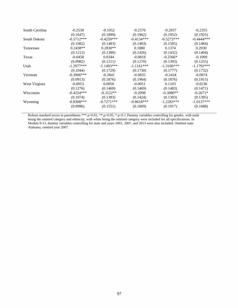
97

South Carolina -0.2538 -0.1052 -0.2576 -0.2937 -0.2355

(0.1647) (0.1899) (0.1962) (0.1952) (0.1925)

South Dakota -0.5712*** -0.4259*** -0.4134*** -0.5273*** -0.4444***

(0.1082) (0.1483) (0.1483) (0.1505) (0.1484)

Tennessee 0.2438** 0.2830** 0.1880 0.1374 0.2030

(0.1212) (0.1390) (0.1426) (0.1432) (0.1404)

Texas -0.0458 0.0344 -0.0818 -0.2566* -0.1009

(0.0982) (0.1211) (0.1270) (0.1393) (0.1255)

Utah -1.2977*** -1.1493*** -1.1161*** -1.3106*** -1.1792***

(0.1044) (0.1729) (0.1730) (0.1777) (0.1732)

Vermont -0.3906*** -0.2841 -0.0835 -0.2434 -0.0974

(0.0913) (0.1876) (0.1964) (0.1876) (0.1915)

West Virginia -0.0053 0.0050 -0.0051 0.1103 -0.0236

(0.1276) (0.1469) (0.1469) (0.1483) (0.1471)

Wisconsin -0.4254*** -0.3122** -0.2098 -0.3080** -0.2671*

(0.1074) (0.1393) (0.1424) (0.1393) (0.1395)

Wyoming -0.8308*** -0.7271*** -0.8618*** -1.2283*** -1.0137***

(0.0996) (0.1551) (0.1609) (0.1917) (0.1688)



Models 9-13, dummy variables controlling for state and years 2001, 2007, and 2013 were also included. Omitted state

Alabama, omitted year 2007.

98

Table A.17: OLS State Regression Results: Determinants of Individual Adolescent log BMI

With State and Year Fixed Effects Model 14 Model 15 Model 16 Model 17 Model 18

Arizona -0.0320*** -0.0302*** -0.0326*** -0.0387*** -0.0338***

(0.0049) (0.0065) (0.0065) (0.0068) (0.0065)

Arkansas -0.0016 -0.0004 -0.0047 -0.0060 -0.0049

(0.0046) (0.0053) (0.0054) (0.0054) (0.0054)

Delaware -0.0070* 0.0010 0.0021 -0.0059 0.0005

(0.0042) (0.0055) (0.0056) (0.0058) (0.0055)

Florida -0.0263*** -0.0220*** -0.0294*** -0.0413*** -0.0286***

(0.0039) (0.0060) (0.0065) (0.0075) (0.0063)

Georgia -0.0092** -0.0062 -0.0077 -0.0123** -0.0071

(0.0046) (0.0051) (0.0051) (0.0053) (0.0051)

Idaho -0.0270*** -0.0233*** -0.0242*** -0.0273*** -0.0239***

(0.0043) (0.0059) (0.0059) (0.0060) (0.0059)

Indiana 0.0030 0.0060 0.0072 0.0060 0.0050

(0.0055) (0.0063) (0.0063) (0.0063) (0.0063)

Kansas -0.0130*** -0.0064 -0.0046 -0.0095* -0.0063

(0.0047) (0.0054) (0.0055) (0.0055) (0.0054)

Kentucky 0.0026 -0.0013 -0.0011 0.0009 -0.0011

(0.0046) (0.0051) (0.0051) (0.0051) (0.0051)

Maine -0.0134*** -0.0134** -0.0066 -0.0089 -0.0077

(0.0040) (0.0061) (0.0064) (0.0062) (0.0062)

Maryland -0.0277*** -0.0208*** -0.0151** -0.0190*** -0.0150**

(0.0037) (0.0065) (0.0067) (0.0065) (0.0066)

Massachusetts -0.0167*** -0.0100 -0.0068 -0.0203*** -0.0081

(0.0040) (0.0072) (0.0072) (0.0076) (0.0072)

Michigan -0.0125*** -0.0051 -0.0060 -0.0088* -0.0063

(0.0040) (0.0046) (0.0046) (0.0047) (0.0046)

Mississippi -0.0093** -0.0174*** -0.0191*** -0.0156*** -0.0177***

(0.0047) (0.0051) (0.0051) (0.0051) (0.0051)

Missouri -0.0108** -0.0060 -0.0059 -0.0099* -0.0062

(0.0045) (0.0053) (0.0053) (0.0053) (0.0053)

Montana -0.0310*** -0.0287*** -0.0305*** -0.0352*** -0.0299***

(0.0039) (0.0060) (0.0060) (0.0062) (0.0060)

New Hampshire -0.0093* -0.0015 0.0076 0.0007 0.0050

(0.0048) (0.0079) (0.0083) (0.0079) (0.0080)

New Jersey -0.0226*** -0.0159** -0.0131* -0.0225*** -0.0130*

(0.0046) (0.0070) (0.0070) (0.0072) (0.0070)

New Mexico -0.0273*** -0.0295*** -0.0352*** -0.0381*** -0.0336***

(0.0042) (0.0069) (0.0071) (0.0072) (0.0070)

New York -0.0198*** -0.0187*** -0.0197*** -0.0339*** -0.0198***

(0.0039) (0.0062) (0.0062) (0.0071) (0.0062)

North Carolina -0.0125*** -0.0087* -0.0094* -0.0135*** -0.0103**

(0.0044) (0.0050) (0.0050) (0.0052) (0.0050)

North Dakota -0.0228*** -0.0247*** -0.0208*** -0.0235*** -0.0214***

(0.0054) (0.0076) (0.0077) (0.0076) (0.0076)

Ohio -0.0105** -0.0093 -0.0062 -0.0079 -0.0086

(0.0052) (0.0058) (0.0058) (0.0058) (0.0058)

Oklahoma -0.0076 -0.0027 -0.0062 -0.0103* -0.0075

(0.0048) (0.0053) (0.0054) (0.0056) (0.0054)

Rhode Island -0.0134*** -0.0131* -0.0066 -0.0133* -0.0073

(0.0043) (0.0074) (0.0076) (0.0074) (0.0075)

99

South Carolina -0.0106 -0.0034 -0.0097 -0.0112 -0.0087

(0.0067) (0.0077) (0.0080) (0.0079) (0.0078)

South Dakota -0.0215*** -0.0153** -0.0148** -0.0196*** -0.0161***

(0.0044) (0.0061) (0.0061) (0.0062) (0.0061)

Tennessee 0.0092* 0.0114** 0.0075 0.0053 0.0081

(0.0049) (0.0056) (0.0058) (0.0058) (0.0057)

Texas -0.0023 0.0016 -0.0032 -0.0105* -0.0040

(0.0040) (0.0049) (0.0052) (0.0057) (0.0051)

Utah -0.0544*** -0.0476*** -0.0462*** -0.0543*** -0.0488***

(0.0043) (0.0071) (0.0071) (0.0073) (0.0071)

Vermont -0.0149*** -0.0104 -0.0021 -0.0087 -0.0027

(0.0037) (0.0077) (0.0080) (0.0077) (0.0078)

West Virginia -0.0011 -0.0007 -0.0011 0.0037 -0.0018

(0.0052) (0.0060) (0.0060) (0.0060) (0.0060)

Wisconsin -0.0156*** -0.0107* -0.0065 -0.0105* -0.0089

(0.0044) (0.0057) (0.0058) (0.0057) (0.0057)

Wyoming -0.0335*** -0.0287*** -0.0343*** -0.0496*** -0.0404***

(0.0041) (0.0064) (0.0066) (0.0079) (0.0069)




Alabama, omitted year 2007.

100

Table A.18: OLS State Regression Results: Determinants of Individual Adolescent BMI With

State and Year Fixed Effects Exclusive of Public School Attendance


Wellness Policy Index 0.0023

(0.0040)

0.0025

(0.0040)

0.0075*

(0.0040)

0.0100**

(0.0040)

Age 0.4286*** 0.4282*** 0.4281*** 0.4282***

(0.0073) (0.0073) (0.0073) (0.0073)

Female -0.7263*** -0.7266*** -0.7266*** -0.7264***

(0.0171) (0.0171) (0.0171) (0.0171)

Days in PE 0.0027 0.0028 0.0031 0.0028

(0.0042) (0.0042) (0.0042) (0.0042)

Black 0.9979*** 1.0187*** 1.0078*** 1.0233***

(0.0337) (0.0338) (0.0337) (0.0338)

Hispanic 0.8540*** 0.8711*** 0.8567*** 0.8837***

(0.0484) (0.0484) (0.0484) (0.0485)

Asian -0.9361*** -0.9142*** -0.9249*** -0.9091***

(0.0477) (0.0477) (0.0477) (0.0477)

Other 0.1835*** 0.2170*** 0.1985*** 0.2222***

(0.0297) (0.0299) (0.0297) (0.0299)

Adult Obesity Rate -0.0004 -0.0024 -0.0374*** -0.0073

(0.0108) (0.0108) (0.0112) (0.0108)

College Education Rate -0.8520** -1.9746*** -1.2664*** -1.3654***

(0.3316) (0.3487) (0.3334) (0.3349)

State Violent Crime Rate -0.0000 0.0003 0.0004* 0.0002

(0.0002) (0.0002) (0.0002) (0.0002)


(0.0088) (0.0088) (0.0088) (0.0088)


(0.3718)


(0.4740)


(0.2697)

Constant 15.9687*** 13.7056*** 14.7428*** 15.6121***

(0.3643) (0.4137) (0.3739) (0.3644)

Observations 243,392 243,392 243,392 243,392

R-squared 0.0363 0.0368 0.0369 0.0368 Robust standard errors in parentheses *** p<0.01, ** p<0.05, * p<0.1; Additional controls include: state dummy variables


About the Author

Anastasia King Smith graduated magna cum laude from St. Petersburg College in St.

Petersburg, Florida with a B.A.S. in Information Technology Management in 2006. In 2010, she

earned an M.A. in Business Economics from the University of South Florida. That same year,

she was accepted into the USF College of Business Ph.D. program and was awarded a graduate

fellowship for her first year of doctoral study. Her fields of study included health economics,

public economics and public health.

As an undergraduate, Mrs. Smith was awarded a National Science Foundation

Scholarship in Mathematics in recognition of academic achievement and as a graduate student

she was employed by the Economics Department as a teaching assistant from period of 2010-

2012. She has been employed with Pfeiffer University as an Assistant Professor of Economics

since 2013.

an exploration of adolescent obesity determinants

Documents