an experimental study of exhaust hydrocarbon emissions ... · pdf filean experimental study of...
TRANSCRIPT

Loughborough UniversityInstitutional Repository
An experimental study ofexhaust hydrocarbon
emissions from a sparkignition engine
This item was submitted to Loughborough University's Institutional Repositoryby the/an author.
Additional Information:
• A Master's Thesis submitted in partial fulfilment of the requirements forthe award of M.Phil of Loughborough University.
Metadata Record: https://dspace.lboro.ac.uk/2134/11135
Publisher: c© N.M.M. Lambert
Please cite the published version.

This item was submitted to Loughborough University as an MPhil thesis by the author and is made available in the Institutional Repository
(https://dspace.lboro.ac.uk/) under the following Creative Commons Licence conditions.
For the full text of this licence, please go to: http://creativecommons.org/licenses/by-nc-nd/2.5/

Pilkington Library
•• Loughborough • University
...................... ..•..•..•...•..••...•.•••.••.....•..•••.••.•......•...••.••..••...•..•..•..
Accession/Copy NO·V
! 0 % :2. ((, 10 i
Vo!. No. ................ Class Mark .. :~:::(tt~';;§.l.§ .................... . .. ,- ," ..: .
001 0825 01
~~\\\\\\\~\\\\\\\\\~~\\~\\\\~\\\\~\~I\~
This book was bound by Badminton Press 18 Half Croft, Syston, .Leicester, LE7 8LD Telephone: Leicester (05331 602918.
'---~-------------~-----.~-.---.
: I .. : j . : I:
: I
I
"
I
\ , , c..-.
\
I
•• Loughborough ., University
A'\l(ington Library
'''-'~-- I'J_N,H ................................. >-- ---- ...• ---- _ •. ---
. ._ 0 _ 0 -1 'L- b : AcCmSION!COf'Y. NO, I --------.- - ------- --- .-- ---- ----- ---_. ---- - - - - - . -- - --
VOL, NO, CLASS MARK
~ 2~.
2 ') "-" I.; _ ,'" .
, l' ~- .• ~ t1QS5 :) ,/-:. ...
0010826 01
-~~IIIIIIIIIIIIIIIIIIII~II~\III~\IIIMIIIII~
This book was bound by
Badminton Press
'.
18 Half Croft, Syston, ,Leicester LE7 8LD Telephone: Leicester (0533) 602918.
L-__ ~ __________ ,, _______________ _
- J JUtRI990
i
i I \ ,-, I , ,
I
I '-

A;\L(ington Library , , ,,_.-'--
•• Loughborough • University
t-J.N.H 'f· ' .................................
. ACCESSION/COPY NO. 'I ." ' "u,01'1-6 .: ------ ----------- ---------- --_ .... _--- - - - - .. - ----
VOL. NO. CLASS MARK
dtvt'.it- cV?K.-, ·t6,
. .' '. ~' . ~ .
001 0826 01
~~\\\\\\\~\\I\\\\\\I\~\\~\\@\\\\M~'\~
This book was bound by
Badminton Press 18 Half Croft, Syston, ,Leicester, LE7 8LD Telephone: Leicester 105331 602918,

1
1
1
1
1
1
1
1
1 .. 1
1
1
1
1
1
1
1
1
1 . 1
1
1 . 1
1
1
1
1
1
1
1
1
1 I
AN EXPERIMENTAL STUDY OF EXHAUST HYDROCARBON EMISSIONS
FROM A SPARK IGNITION ENGINE
by
N. M. M. Lambert
A Masters Thes is
Submitted in Partial Fulfilment of the Requirements
for the Award of
Master of Philosophy of Loughborough University of Technology
May 1986
SUpervisor: Professor J.C. Dent, Ph.D., C.Eng.
© by N.M.M. Lambert 1986
j
j
j
j
j
j
j
j
j
j
j
j
j
j
j
j
j
j
j
j
j
j
j
j
j
j

SUMMARY
The control of hydrocarbon emissions from spark ignition engines is
important and there is a need for a better understanding of the
mechanisms contributing to this source of emissions.
The absorption/desorption mechanism is believed to be a significant
contributor to hydrocarbon emissions. The aim of the project has been
to validate the absorption/desorption model experimentally.
Modelling studies predict that sufficient fuel vapour is absorbed
into the cylinder wall oil film on the compression and early firing
strokes with subsequent desorption late in the expansion stroke to
seriously affect hydrocarbon emissions in the exhaust, as
temperatures are too low for adequate oxidation.
The experimental investigation which follows develops a method to
allow accurate measurement of hydrocarbon specie levels in the
exhaust of a spark ignition engine. The object of the experiment was
to detect and measure differences in hydrocarbon levels for two
fuels, Iso-octane and Iso-pentane, at identical engine conditions and
therefore establish whether the absorption/desorption effect is
significant to hydrocarbon emissions. The theory behind this relies
upon the varying solubilities of both fuels in a given oil with
temperature wh ich shoul d refl ect a varyi ng base fuel hydrocarbon
emissions level for each fuel if absorption/desorption is in fact
taking place.
Samples of exhaust were taken from a Ricardo-hydra test engine and
analysed chromatographically. Experimental results (which compare
favourably with prediction from modell ing studies) indicate about 30
i

•
percent of total hydrocarbons are due to the absorption/desorption
rnechan i srn.
In conclusion, the results suggest that the solubility of the fuel in
the engine oil has a significant effect on hydrocarbon levels in the
exhaust.
i i

ACKNOWLEDGEMENTS
I woul d 1 ike to thank my research supervisor, Professor J.C. Dent,
for his advice and guidance throughout the course of this work.
My thanks are also expressed to the technician staff of the
Mechanical Engineering Department with special thanks to
Mr. G. Manship, Mr. S. Line and Mr. S. Taylor who struggled to build
equipment with limited resources.
I wish to express my sincere thanks to colleagues and friends whose
assistance has helped the completion of this thesis.
Appreciation is also due to the Shell Oil Company and the Chemical
Engi neeri ng Department of Loughborough Univers ity of Technology for
the loan of equipment vital to this project.
Finally I must acknowledge the financial help of the Ford Motor
Company who have made this research possible.
i i i

Index of Contents
SUMMARY
ACKNOWLEDGEMENTS
CHAPTER 1
LITERATURE SURVEY
Introduction
1.1 The Effect of Quench Layers and Crevices
on Hydrocarbon Emissions
1.2 The Effect of Engine Variables
on Hydrocarbon Emissions
1.3 The Effect of Fuel Composition
on Exhaust Hydrocarbons
1.4 Depos it Format ion - It's Effect
upon Exhaust Hydrocarbons
1.5 The Effect of Oil Layers
on Hydrocarbon Emissions
CHAPTER 2
EXPERIMENTAL METHOD
2.1 Introductory Account
iv
Page
1
i i i
1
3
7
10
12
14
21

2.2 Typical Engine Test
2.3 Exhaust Sample Analysis
2.4 Chromatographic Method
2.5 Ca 1 i brat i on Procedu re
2.6 Data Reduction
CHAPTER 3
EXPERIMENTAL ACCURACY AND IDENTIFICATION
OF HYDROCARBONS - DISCUSSION
3.1 Experimental Accuracy
3.1.1 General Note
3.1.2 Engine Conditions
3.1.3 Hydrocarbon Mass Calculation
(Wei ghi ng Method)
3.2 Identification of Hydrocarbons
CHAPTER 4
EXPERIMENTAL EQUIPMENT
4.1 Sampling Flask System
4.2 Air Intake System
v
Page
23
26
27
29
33
35
35
35
36
38
40
43

Page 4.3 Fuel System 45
4.4 Gas Chromatograph 47
4.5 Electronic Integrator 48
4.6 Exhaust Gas Analyser 51
4.7 Ignition System 54
4.8 Injection System 55
CHAPTER 5
GENERAL DISCUSSION OF RESULTS AND CONCLUSIONS
5.1 Discussion of Results and Figures 56
5.2 Concl us ions 62
CHAPTER 6
REFERENCES AND APPENDICES
REFERENCES 65
APPENDIX A - Engine Test Conditions 70
APPENDIX B - Chromatographic Data 71
APPENDIX C - Engine and General Specification 72
APPENDIX D - Typical Hydrocarbon PPM C Levels 73
vi

APPENDIX E - Program Listing (Calculation of Air/Fuel Ratio)
APPENDIX F - Data Reduction Program
APPENDIX G - The Effect of Crevice Volumes on Base Fuel Hydrocarbon Emissions for Iso-octane and Iso-pentane
APPENDIX H - Henry Constant Test
APPENDIX I - Engine Test Data Tabulated
APPENDIX J - The Solubilities of Iso-octane and Iso-pentane in Squalane
vii
Page
74
78
83
87
91
92

CHAPTER 1
LITERATURE SURVEY

CHAPTER 1
LITERATURE SURVEY
Introduction
The gasoline engine is a major source of air pollutants and the
problem has been tackled so that emissions are minimised in both the cyl i nder and subsequently through suitable after treatment of the exhaust ga se s.
The three independent sources of air pollutants include:
(1) Crankcase blowby
(2) Evaporative emissions
(3) Exhaust emissions
This report is concerned only with the third case and specifically with unburned exhaust hydrocarbons.
It is now generally accepted that the main sources of unburned
hydrocarbons from spark ignition engines are:
(1) Flame quenching at the walls of a combustion chamber.
(2) Unburned fuel in the various trapped vol umes inside the combustion chamber (ie. top piston land, around spark plug and ring
crevices) •

(3) Gas phase quenching when the engine is running under extreme
conditions of stoichiometry.
(4). Absorption/desorption in the cylinder lubricating oil films and
surface deposits
The fi rst three are fai rly well understood and documented[1-
9],[13],[15],[21]. The absorption/desorption process being a
relatively new concept very little literature has been published.
Combustion test data[23],[24],[27],[28] and mathematical
modelling[10],[26] suggest the possibility of the
absorpt i on/desorpt i on mechani sm bei ng a sign ifi cant sou rce of
unburned hydrocarbons. Consequently the need for a representative
experimental method to support the theoretical evidence.
Discussion of the various investigations which follow will be
focussed mainly on the absorption/desorption source and so most
literature cited will be confined to this area.
2

1.1 The Effect of Quench Layers and Crevices On Hydrocarbon Emissions
Quench layers are believed to be regions of unburned fuel, close to the wall s of the combustion chamber, owing to the flame quenching short of the combustion wall. Crevices or trapped volumes can be defined as any volume into which the flame cannot propagate.
Lorusso et al[l] used a gas sampling valve in the combustion wall of a spark ignition engine to sample hydrocarbons near the wall over a
wide range of engine operating conditions. Experimental results
suggested that quench layer hydrocarbons contributed no more than 3 -12 percent of the total hydrocarbons observed in the exhaust and therefore indicated that the other sources :- ring-crevice storage, absorption-desorption and surface deposits were more important. Figure(l.l) shows volumetric concentration in parts per million (ppm) at the cyl i nder wall for various hydrocarbon species at different crank angles. It can be seen that there is a low level of quench
layer hydrocarbons at 40 degrees crank angle which represents the actua 1 contri but i on due to quench 1 ayers. The ri si ng port ion of the hydrocarbon concentrations after 40 degrees is believed to result from convection of unburned material into the sampling zone from sources other than wall quenching(ie., ring crevices, oil films,
etc) •
Recent combustion bomb experiments by Adamczyk et al [2] have
supported the theoretical results of Westbrook et al [3] showing that wall quench hydrocarbons are extensively burned after the time of flame quenching at the walls. Furthermore, the exhaust hydrocarbons under stoichiometric conditions are shown to be 95
percent fuel molecules with few product gases present, indicating little exposure to high temperature oxidation processes. Adamczyk et
al[2] also demonstrated the significance of crevices as a source of hydrocarbons but conclude that with rich mixtures(equivalence ratio
of 1.4) and for a clean vessel, storage volumes and wall- quenching cannot account wholly for all the exhaust hydrocarbons.
3

Daniel and Wentworth[4] presented evidence to show that wall quenching is the fundamental source of exhaust hydrocarbon emissions from a spark ignition engine, but further work[5] since then has
poi nted to the exi stence of a spec i a 1 case of the quench phenomenon which is now understood as the "crevice effect". Wentworth[5] showed that by using the sealed ring-orifice(SR-O) design which minimised the crevice effect, exhaust hydrocarbon concentrations were reduced
significantly. In the SR-O design the piston and top compression ring in an engine are modified to virtually eliminate the crevice between
the top land and the cylinder wall, and at the same time, seal the combustion chamber at the top compression ring. Wentworth[6] gives extensive details of the SR-O design. Experiments by Wentworth[5] with a single cyl inder engine showed that small crevices formed by
the piston, bore and top compression ring were responsible for at least half of the exhaust hydrocarbon emissions in a clean engine for
most conditions of speed and load. Further work by Wentworth[6] confirmed the importance of the piston crevice volume effect on
exhaust hydrocarbon emissions. Experiments were carried out using a revised design of spark ignition engine piston having a much narrower
top 1 and and reduced hydrocarbon 1 evel s by about 50 percent on the
production design. These results demonstrated the sizeable reductions in exhaust hydrocarbon emission that are possible when the pistonbore-ring crevice volume is essentially eliminated.
Daniel[7] analytically modelled the effect of engine variables on . exhaust hydrocarbon emissions to compare quench layer and crevice
volume sources. The data, Figures(1.2) & (1.3), indicate that crevice volume sources produce much greater changes in unburned hydrocarbons than quench layer sources for all engine variables
considered. This lends further weight to the belief that quench layers are an insignificant source to exhaust hydrocarbons.
Weiss and Keck[8] carried out a time resolved study of the unburned hydrocarbons in the cylinder of a spark ignition engine and considered just two sources of hydrocarbons: quench layers and
4

crevice volumes. For the purposes of comparison samples of hydrocarbons were collected from both the cyl i nder, us ing a needl e val ve, and the exhaust. Model s were developed for predict ing hydrocarbons from both quench 1 ayers and crevice vol umes. The data presented concluded, that of the two sources considered crevice volumes were the only significant contributor to exhaust hydrocarbons. Quench layer hydrocarbons mixing with the burned gas
were shown to be completely oxidised due to the sufficiently high
temperatures prior to blowdown.
Single-Pulse sampling valve measurements of wall layer hydrocarbons in a combustion bomb by Adamczyk et al[9], have shown that less than
10 percent of tail pipe emissions can be attributed to the quenching process. Propane and air were used as the fuel and oxidiser with a fuel lai r equival ence ratio of 0.9. The sharp drop in propane
concentration coupled with the sharp rise in propane oxidation products supports the theory that the fl ame quenches short of the combustion wall. Residual Propane in the wall quench layer is free to
diffuse into the hot bulk gas forming intermediate products which are then consumed about 4 milliseconds after flame arrival.
The results, Figure(1.4), show how the Propane concentration changes with distance from the wall, where increasing the sampled mass(which is effectively sampling at an increasing distance from the wall)
causes hydrocarbons to diminish. For a short time after flame arrival, up to about 200 milliseconds, the decrease in Propane
concentration with increasing distance from the chamber wall is quite marked. However at about 400 milliseconds there is only a relatively small change in concentration with distance from the wall. This higher Propane concentration - above exhaust concentration - could be attributed to material diffusing into the wall region from a source such as a crevice or even desorption from an oil layer. The
measurements suggest that the adjustment of hydrocarbon level in the quench layer could be controlled by crevice volumes. It is also indicated that a fraction of the exhaust background hydrocarbon level may arise from a residual of the quenching process. Moreover through
5

measurement of the hydrocarbon concentration of the residual gases
Daniel and Wentworth[4] established that a significant proportion of
the quench zone hydrocarbons may be recycled within the engine •
•
6

1.2 The Effect of Engine Variables On Hydrocarbon Emissions
The effects of engine variables on exhaust hydrocarbons have been investigated both through mathematical modelling[10],[7] and experiments[11],[12]. Lavoie et al[13] analysed these effects through modelling and experimental methods in terms of ring crevice and wall
quench hydrocarbon contributions. Predicted and experimental data compared well for hydrocarbons versus indicated specific fuel consumption, indicated mean effective pressure, compression ratio and exhaust gas recirculation(EGR) but poor correlation was shown for
hydrocarbons versus coolant temperature, engine speed and equivalence ratio (rich). Owing to the discrepancies between the models and
experiment it was concluded that further work was necessary to elucidate the processes of wall quenching, ring crevice storage and
blowby effects.
A single cylinder engine study was carried out by Wentworth[14] (using a sealed ring - orifice piston[6] as described earlier) to quantify the effect of combustion chamber surface temperature on
exhaust hydrocarbon concentration. Figure(1.5) shows the relationship between exhaust hydrocarbon emissions and cylinder surface temperature. Simultaneous measurements of combustion chamber surface temperatures and exhaust hydrocarbon concentrations in a single cylinder spark ignition engine showed that about 43 percent of the drop in hydrocarbon level was due to increased surface temperature. After considering the way in which other engine variables(such as pressure, engi ne speed, turbul ence etc.) may effect the hydrocarbon level no satisfactory explanation was found for the other 57 percent
drop.
Engine variable effects on exhaust hydrocarbon composition were
investigated by Daniel[ll] using a single cylinder engine with
Propane as the fuel. It was found that an engine variable effect observed at one air-fuel ratio, ignition timing combination was not
7

necessarily directionally the same as that observed at another ai r
fuel ratio, ignition timing combination. The data showed that:
(1) the minimum total hydrocarbon concentration was obtained at a
lean air-fuel ratio
(2) retarding the timing reduced the total hydrocarbons
(3) increasing engine speed reduced hydrocarbons generally
(4) increasing the compression ratio increased the total hydrocarbons
(5) increasing the exhaust back pressure decreased the total
hyd roca rbons
(6) increasing the temperature decreased the total hydrocarbons
Figures(1.6) - (1.12) clearly indicate the above effects.
For all engine variables the concentration of Propane found in the
exhaust behaved in the same way, directionally, as the total
hydrocarbon concentration. However Daniel's experiments failed to
show the relative importance of the engine variables which affect
both the amount and composition of the exhaust hydrocarbons.
Additionally the data did not indicate how fuel and non fuel
hydrocarbons may be affected differently by changes in the proportion
of total hydrocarbons exhausted.
Namazian and Heywood[15], using a single cylinder square pistoned
engi ne, demonstrated that unburned hydrocarbons bl eeding out of the
top ring gap can affect exhaust hydrocarbon emissions and that the
location of the ring gap with respect to the spark plug and exhaust
va 1 ve is important. The squa re-cross-sect i on engi ne was fitted with
two parallel quartz glass walls which permitted optical access to the
entire cylinder volume. In this way gas flow into and away from the
top ring gap could be photographed and details of the flow examined
8
closely. The test results showed that for the spark plug located near
the exhaust valve, placing the top ring gap 90 degrees away produced
lowest emissions. A gap too close to the exhaust provides an easy
path for trapped hydrocarbons to exit. Pl acing the gap 180 degrees
away maximised hydrocarbons. In general, the closer the plug was to
the exhaust valve the lower were the hydrocarbon emissions. The
authors[l5] bel ieved that this may have been because of the greater
residence time for hydrocarbon burn-up and the selective exhausting
process of the cyl inder. Lowest emissions were obtained with dual
ignition, and ring gap position had little effect in that case.
Experiment therefore confirmed that crevice gases constitute a major
source of unburned hydrocarbon emissions as well as a significant
loss in power and efficiency.
9

1.3 The Effect of Fuel Composition on Exhaust Hydrocarbons
Dishart and Harris[16] conducted exhaust emission measurements using
gasolines of varying aromatic and olefin content in a variety of
vehicle types and concluded that no significant changes in total
hydrocarbons in the exhaust would result from changes in gasoline
hydrocarbon composition. In contrast R.D. Fleming[l7] later found
that fuel composition does affect exhaust emissions from a spark
ignition engine. In the investigation[l7] a single cylinder research
engine was run on three pure hydrocarbons found primarily in
commercial fuels, namely a paraffin(2,2,4-trimethylpentane), an
01efir(2,4,4-trimethylpentene-2) and an aromatic(metaxylene). The
exhaust samples were analysed for carbon monoxide, carbon dioxide,
hydrogen, nitrogen oxides, aldehydes and hydrocarbons. A detailed
study was made on the post combustion reactions for each fuel from
the analysis of the exhaust ·products.
Amongst the three fuels which Fleming[17] assessed, it was found that
the paraffin fuel gave the highest total hydrocarbons in the exhaust
while the aromatic produced the highest base fuel hydrocarbon level
in the exhaust. Infact for the same conditions the base fuel level
for the aromatic was three times that for the paraffin. This was
expected since the ring structure of aromatics is quite stable
producing less decomposition than for the case of the paraffin. From
this Fleming concluded that as aromatic content in fuel is increased,
the hydrocarbon mole fraction of aromatic in the exhaust that
represents unburned fuel increases.
An explanation for the discrepancy between Dishart and Harris and
Fleming's conclusions may be offered in terms of the fuel blends used
in the experiments. Dishart and Harris used complex fuel blends made
up of various hydrocarbons while Fleming kept to single component
fuels and simple two component mixtures of pure hydrocarbons. It is b'
therefore theo~ized that any isolated component effect on emissions, ,.
in a compl ex fuel bl end, is 1 i kely to be masked by effects from the • , . .-
10

other components within that blend. For this reason it is suggested that Fleming's method of investigating each component's effect on
hydrocarbons in isolation is the most practical method of assessment
rather than the global method adopted by Dishart and Harris.
11

1.4 Deposit Formation - It's Effect Upon Hydrocarbons
Published experimental data on deposit formation as a source of exhaust hydrocarbons is scarce. Although combustion chamber deposits
are known to increase exhaust hydrocarbon emissions the relative contributions of deposits from various parts of the chamber still
requi res further invest i gat ion. Wentworth[l8] performed experi ments to assess the significance of wall deposits on exhaust hydrocarbons
at various locations in an engine. It was found that deposits exhibit a location effect and therefore contribute different increments to exhaust hydrocarbon concentration.
Data[18] was collected for deposits at various locations in the
chamber and indicated that the average hydrocarbon concentration increase, 25 ppm, was more than 10 times the smallest increase, proving that deposit location has considerable influence on the contribution that deposits make to exhaust hydrocarbon concentration. Generally it was found that deposits in the vicinity of the exhaust valve produced greater hydrocarbon increases than for any other location in the combustion chamber. The reason for this was assumed to be due to the direction of swirl induced by the intake charging process, so that hydrocarbons clinging to the wall surfaces somewhat
"upwind" of the exhaust valve would most likely be exhausted.
It is stressed that deposits are not the only source of hydrocarbon emission which might exhibit location effects. Hydrocarbons
originating at different portions of clean wall surfaces, as well as hydrocarbons originating in different portions of crevice, may
contribute different increments to exhaust hydrocarbon concentration because of their particular location in the combustion chamber.
Jackson et al[19] also studied the effect of combustion chamber wall deposits on exhaust hydrocarbons experimentally and concluded that the accumulation of deposits in both a single cylinder and multicylinder engine,Figure(l.13), caused a significant increase in
12

exhaust hydrocarbon content. Therefore it appears that engine deposit condition is an important factor which cannot be neglected in making
long term comparative tests or in establishing absolute levels of exhaust hydrocarbon emission from engines.
13

1.5 The Effect of Oil Layers on Hydrocarbon Emissions
There is increasing evidence to suggest that cyl inder oil layers in
spark ignition engines could be a significant source of exhaust
hydrocarbons.
Haskell and Legate[20] first theorized that the effect of oil on
exhaust hydrocarbon concentrat ion coul d be due to ·momenta~y_
absorption of fuel vapour into the oil film coating the combustion
chamber wall. Moreover, it was suggested that the decrease in
hydrocarbon concentration resulting from increased coolant
temperature[l4] was due to decreasing solubil ity of fuel in the oil
film. The effect of the absorption/desorption phenomenon on exhaust
hydrocarbons was extens i vely modell ed by Dent and
Lakshminarayanan[10] and compared with existing experimental data.
The predictions of the model compared favourably with engine
experiments(Lavoie et al [13] and Lavoie and Blumberg[21]) for
different engi ne vari abl es apart from exhaust gas reci rcul at ion(EGR).
In contrast the predicted data presented by Lavoie et al [13]
generally fell short of the experimental data for hydrocarbons
versus coolant temperature,engine speed and rich equivalence ratios.
The absorption/desorption mechanism assessed in Reference [la] has
essentially accounted for these discrepancies between experiment and
model. Dent and Lakshminarayanan[10] conclude that the two major
sources of hydrocarbon formation are crevice volumes and cyclic
absorpt i on/desorpt i on. The p roces s of abs orpt i on a nd des orpt i on of
fuel vapour into the oil film layer is illustrated diagrammatically
in Figure(l.14). It has been theorized that transfer of fuel vapour
across the oil film layer is by molecular diffusion and a linear
concentration gradient in the oil has been assumed. An effective
penetration depth, the controlling factor of this mechanism, has also
been assumed. It is dependent upon the following parameters:
(1) The fuel/oil combination(ie.,the Henry Constant for the
14

particular combination will affect the solubility of the fuel in the
oil and so affect the amount of absorption taking place).
(2) Engine speed(ie.,Since fuel/oil absorption and desorption is time
dependent engi ne speed wi 11 be inversely proport ional to the
penetration depth).
(3) Engine 10ad(ie.,The rate at which fuel is transferred into the
oil is controlled by cylinder pressure. The higher the cylinder
pressure the greater the absorption rate).
(4) Coolant temperature(The Henry Constant of the fuel in the oil
falls - while solubility increases -with increasing coolant
temperature. This results in less absorption of fuel into the oil).
All the variables discussed above have been shown to effect the level
of hydrocarbon emissions in the exhaust[10],[13],[11].
The effect of varying wall temperature on hydrocarbon emissions,
Figure(l.15), is primarily due to variation of Henry Constant and
variation of oil viscosity with temperature. In addition increasing
wall temperature reduces gas density in the trapped volumes and so
decreases crevice mass contribution to hydrocarbon emissions. The
importance of absorption/desorption as a significant source of
hydrocarbons is compared to ring crevice contribution. Experimental
data[13] are also shown in the figure for comparison. It is evident
that for relatively high coolant temperatures, such as 360 K and
above, the model proposes that the absorpt ion/des orpt i on mechan i sm
accounts for at 1 east 50 percent of the total hydrocarbons in the
exhaust.
Figure(1.16) indicates the instantaneous level of hydrocarbons in the
oil layer with crank angle for the first engine cycle. Early in the
induction stroke, when cylinder pressure is sub-atmospheric, a low
15

level of hydrocarbons( fuel vapour) are found dissolved in the oil
layers. This hydrocarbon level increases with the compression and expansion strokes reaching a maximum shortly after top dead
centre(TOC) where cylinder pressure is also at a maximum. This level diminishes as cylinder pressure falls finally reaching a minimum at the end of the exhaust stroke. The trend with cylinder pressure is to be expected since absorption and desorption are related directly to
the Henry Constant and the mass transfer conductance[10]. The quantity of fuel vapour remaining in the oil at the end of the cycle
is dependent upon the period of the cycle(ie.,engine speed) and the thickness of the oil film. This residual of fuel at the end of the
first cycle forms the initial condition for the next cycle which generates a slightly greater fuel residual and for subsequent cycles there is a build up of fuel mass in the oil film, Figure(1.l7), until an equilibrium state is reached where absorption/desorption fluctuates about a steady periodic level. Also shown, Figure(1.17), is the variation of net hydrocarbons desorbed after oxidation with crank angle which demonstrates the cyclic nature of the mechanism. It is seen that desorpt ion starts about 90 degrees after top dead centre(ATOC) on the expansion stroke and increases rapidly to reach a
maximum at about BOC. This behaviour is due to three factors. Firstly the oil film temperatures are below 1100 degrees K and therefore oxidation of the desorbed hydrocarbons is negligible. Secondly, the surface area for desorption increases as the expansion proceeds, and finally the decrease in cylinder pressure during expansion causes an
increase in the Henry Number which results in an increased desorption rate. Beyond bottom dead centre during the exhaust stroke desorbed hydrocarbons decrease because of the reducing surface area for desorption.
The model[10] discussed above has two limitations. Firstly it assumes a uniform oil film thickness on the cylinder wall surface. Oil film thickness on the piston ring has been measured during an engine run by Keiichiro Shin et al[22] and it was found that with standard ring arrangements the thickness of oil formed on the top ring was appreciably smaller than the theoretical value. This was attributable
16

to the inadequate supply of lubricating oil to the ring.Therefore
since the absorption/desorption mechanism is dependent on oil film
thickness[23],[24] the magnitude of this effect predicted by the
model[lO] would be lower in value(ie. less than the 50 percent
indicated). Secondly the engine lubricant was assumed to be squalane
since data was readily available for Henry Constants for various
paraffins dissolved in squalane over a range of temperatures[25]. n
Octane was used as the fuel and its Henry Constant in squal ane found
by extrapolation of data given by Chappelow & Prausnitz[25]. It was
accepted that the process of extrapolation is prone to error and that
the use of n-Octane as the fuel instead of Iso-octane(which is more
representative of commercial fuel) could introduce error due to their
differing solubil ities.
Carrier et al [26] also investigated this cyclic effect of the
absorption/desorption mechanism by theoretical modelling. The model
was intended to approximately duplicate the hydrocarbon
absorption/desorption effect in the oil film layer on the cylinder
wall of a reciprocating piston engine. It was found to be consistent
with experimental data[ll],[13],[21] demonstrating the
absorption/desorption effect on hydrocarbons, which decrease with
increasing engine speed, as shown in Figures(1.18) & (1.20). It is
also indicated that first cycle absorption (Figure(l.19)) is greater
than the absorption/desorption of a steady periodic
level(Figures(1.18) & (1.20)). At the same time it was shown that
first cycle desorption was less than the absorption/desorption of a
steady periodic level.
The model[26] revealed that solubility increases with pressure in the
cylinder. Although the model had considered the reciprocating nature
of the piston engine it had ignored flow within the oil film, the
combustion event was taken as instantaneous and the variabil ity of
Henry's Constant with pressure was also ignored. The model was
concerned with total .hydrocarbons rather than the discrete
components, so no predictions could be made on how the various
hydrocarbon specie were being affected.
17

The effect of oil layers on hydrocarbon emissions has been
investigated by Kaiser et al [23]. Measured amounts of oil were placed on the piston of a CFR engine fuelled on Propane, and Iso
octane. It was evident(Figure(1.21» that when fuelled on Iso-octane, measured quantities of oil added to the engine cylinder produced proportional increases of the base fuel in the exhaust hydrocarbons. When the engi ne was fuel 1 ed on Propane, base fuel concentrat ion in
the exhaust hydrocarbons was significantly lower than in the Isooctane case. In fact in the Propane fuelled case the hydrocarbon distribution was essentially constant with or without oil added, indicating that burning up of the oil itself was not contributing to
the higher base fuel hydrocarbon level when running on Iso-octane.
It was found by Kaiser et al [23] that the exhaust hydrocarbons (base
fuel) increased with increase in the volume of oil deposited on the piston. The tempe ratu re dependence of fuel /oi 1 solubil ity was al so demonstrated, higher temperatures producing lower levels of base fuel hydrocarbons. The effect of oil temperature on solubility and diffusion rate of the fuel in the oil was not assessed because of unknown surface temperatures and loss of oil from the cylinder. However it was concluded that the principle source of increase in
hydrocarbon concentration was the dissolving of the fuel into the oil layer during compression, with subsequent release into cooling burned gas during the expansion stroke.
Adamczyk and Kach [24] studied the problems of absorption/desorption
using low solubil ity oils. A combustion bomb was used to show how hydrocarbon emissions vary with 5 different oils in ascending order of Henry Constant (squalane, a synthetic motor oil, a petroleum-based motor oil, a polypropylene oxide oil and a polypropylene-polyethylene oxide copolymer oil) in combination with 3 different fuels (Ethane, Propane and Butane). Glycerol of higher Henry Constant than the oils
was also studied with Propane as the fuel. The experimental results showed that hydrocarbon emissions varied in direct proportion to the quantity of oil present in the bomb, to the initial fuel
18

concentration and to the solubil ity of the specific fuel in the oil
layer (Figures(l.22) & (1.23)). Not surprisingly, increasing the wall
temperature decreased the hydrocarbon emission. In conclusion the
results indicated that the oil 1 ayers do significantly increase the
hydrocarbon emission and that this increase is extremely dependent on
the specific fuel/oil combination. The primary hydrocarbon emission
from the exhaust was found to be unreacted fuel.
Kaiser et al[27] demonstrated the effect of oil layers on the
hydrocarbon emissions generated during closed vessel combustion. This
was done by analysing, chromatographically, the exhaust gas from a
combustion bomb generated with and without the presence of oil. Five
fuels (Methane, Ethane, Propane, n-Butane and Hydrogen) and three
oils (a synthetic motor oil, a petroleum based motor oil and a
diffusion pump fluid) were used at a variety of fuel/air equivalence
ratios. The results showed that for an equivalence ratio of 0.9, the
higher the carbon number of the fuel the greater the hydrocarbon
emissions (i.e. hydrocarbons of higher molecular weight are more
soluble in oil than those of lower molecular weight).
Figure(1.24) illustrates this effect clearly. The experiments
indicated that the exhaust hydrocarbon concentration was made up of
at least 95 percent of base fuel at fuel lean conditions and was
proport i ona 1 to the amount of oi 1 in the bomb and the sol ubi 1 i ty of
the specific fuel in the oil. However for rich conditions,
equi val ence rat io greater than one, hydrocarbon emiss ions were very
much greater and made up of 1 ess than 1 percent of base fuel. The
reason for this was shown to be due to degradation of the oil into
1 i ghter hydroca"rbons wh ich was dependent on equi val ence rat io and
fuel type. From the data it was evident that both crevice volumes and
the absorption/desorption mechanism play an important part in exhaust
emission generation and that post desorption oxidation is minimal.
A further combustion bomb study of fuel-oil solubility and
hydrocarbon emissions from oil layers was carried out by Adamczyk and
Kach[28]. The bomb study estimated the solubility of four fuels
19

(Methane, Ethane, Propane and n-Butane) in squalane over a range of
temperatures (298 K - 382 K). All experiments were performed at a
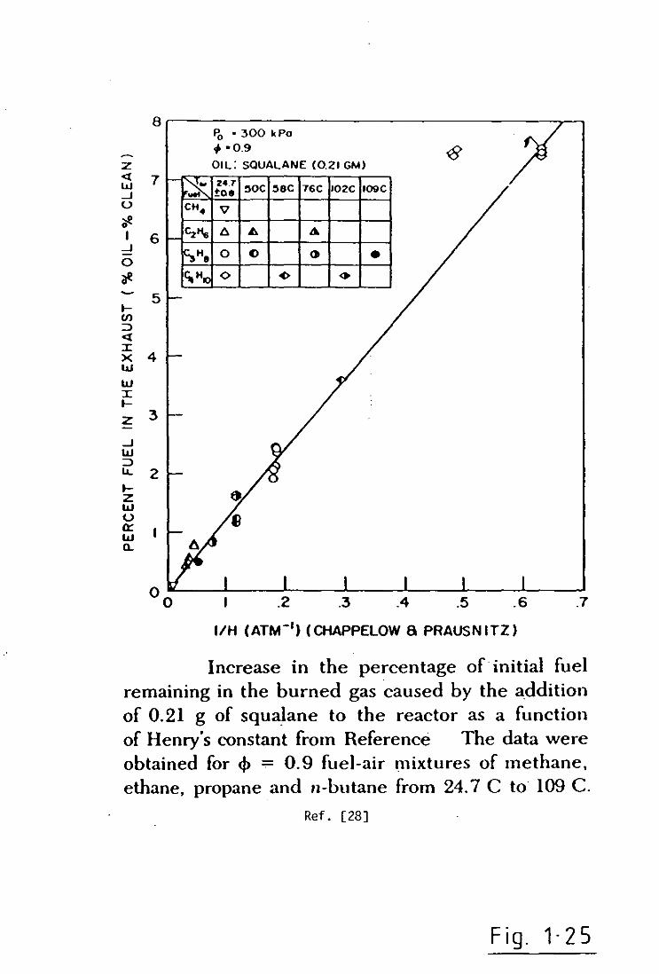
fuel-lean equivalence ratio of 0.9. It was shown, Figure(l.25), that
hydrocarbons vary inversely with Henry Constant over an order of two
magnitude change in the value of Henry Constant. This trend is to be
expected since so I ubil i ty vari es inversely to Henry Constant, Methane
with the greatest Henry Constant is the least soluble of all the
fuels and n-Butane possessing the lowest Henry Constant is the most
soluble of the four fuels tested. Note that, although the data for
n-Butane at room temperature (the unfilled diamond shaped paints)do
not lie on a straight line through the other data, the difference
between the straight line and this data was believed to indicate an
inconsistency in the value for Henry Constant for n-Butane in
Squalane reported by Chappelow & Prausnitz[25]. Appropriate
extrapolation of this data[25] for a room temperature condition
yielded a new value of Henry Constant for n-Butane giving the flagged
points in Figure(1.25) which lie directly on the plotted data line.
It has been demonstrated that the absorption/desorption of fuels into
oil layers can occur on engine time scales and can significantly
increase the hydrocarbon emiss ion from a homogeneous charge engi ne.
The results indicated that the magnitude of the exhaust hydrocarbon
emissions from a non-degrading oil layer during clean combustion are
directly related to the solubility of the fuel in the oil. However
the study did not show the direct relationship between the magnitude
of the oil layer hydrocarbon emissions and fuel-oil solubility.
20

~
0:: lLI >-« -' :c u z lLI ::0
= '-'
E '0. a.
Z 0 ;= <t 0::: I-z w u z 0 U
1'0'
let
103
10z -
10
0.1
-2.0
O·
CO2
02
CO
C3 H.
9 CH2 0
0.0 2.0 4.0 6.0
" CH. 6C2~ OCzH. +C3H,; OC3He OCHZO • CH3CHO 11 CZHsCHO eco o CO2 .... 0 2
(CzKo)
• (C 3 H6 .czH2·CH4)
80
61, - TIME AFTER FLAME ARRIVAL (m.eel
20· AO· 60·
CRANK ANGLE (DEGREES ATDC)
10.0
80·
Exp3ndcd plol of hydrocarbon .pecies. CO •• CO and 0. concentrations measured nczr the time of (b.rne arrival at the sampling valve location ror ~=O.9. basclinemgine conditions. Species concentrations are plotted vc.-sus the time after flame arrival. ~, and «:ank an~lc degrees ATDC. Sample mass per cycle. ll.nr= 7.6 x 10-- g. Symbols with downward arrow represent values at or below the dctection limit. .
Ref. [1]
Fig.1·1

"
AIR-fUn RATIO
.. I~
.----.~
COMPRESSION RATIO
. !-; --~-~,'"
___ a
0_0
IGNITION TlMINC
.0 10 tlX tUJlfit D(GltttS ITC
/ ./
AIR-flOW RAT!
0--.,--------------,
, .. EJ<CIt« SPlIO
... .,,,
Variations in unbumcd propane due to flame quenching with engine variable changes
Fig_ 1 2
110··,--------------------,
I~
'''', "". AIR-fUD. RATIO
:. 11
COMPRESSION RATIO
',,--'" •
ICNITION TlMINC
10 ,0< CRANt O[~m tTt
AIR-flOW RAT!
.. 10
to 'Ull fHltOnll
• \.
"'-•
[NCIt« SPErO
...
Variations In unburned propane due to chamber crevices with engine variable changes
.Ref. [7]
Fig.13

103~------~------~------~------s-,
~ 0.. 0..
Z o ~ 10
2
0::: IZ W U z 8 101
w z « 0.. o 0:::
, ~~tJ
__ t = 15 MSEC. ~~ii---"" --A-- t = 80 MSEC. . ~'" -0- t = 170 MSEC. ~ ''A -.~.- t =400 MSEC. . ,
~ ~-G \ Pa= 200 k Pc
cp = 0.9
\ \
\J~ \ \
0.. 100 ~ ______ ~ __ ~ __ ~ ______ ~~ __ ~ __ ~~
10-6 10-5 10-4 10-3
b.M (SAMPLFD MASS,GM)
PROPANE CONCENTRATION AS A FUNCTION OF SAMPLED MASS
AT 15. an. 170 AND 400 MSEC AFTER PEAK PRESSURE~ [Ref. 9]
Fig. 1· 4

SPEED, 800 RPM INTAKE DEPRESSION, 12 IN~ HG
SPARK TIMING, 22 DEG. BTC 180 •
\ -0 L>
=E COOLANT Cl... .\ Cl... 160 • WATER . o ETHYLENE GLYCOL L> z • 0
'" L>
Z 0 140 • co "0 0::
'" « L> 0 0:: .0"", Cl >- 120 :c I-
~ V)
" ~
« 0" :c
x 100 UJ 0 "-0
160 200 240 280 320 AVG. SURFACE TEMP., OF
The effect of average surface temperature on exhaust hydrocarbon concentration-varying coolant temperature [Ref. 14]
Fig.1·S

·'~,----~.----:,,----:,,----~~~--~n~---!~
Effect of air· fuel ratio on total hydrocarhon con· centration
.. '"
! ~
.. i la
~
" > lID
..
Fig. 1· 6
NI '''' 15.1 2G ... I ... . IU 1 ll.) •
"'-. . "-." .~ . . ...... "~."."-. . ...... ~--=
'. ------_. . . . .-....... " .,- .. ............ ---...---.
"X.. .,.-._. ""'" -.. - . ........... --. ---...... ..
111&1" )1110 • __
l~rrCt:t "r CIIl)iIlC ~pccd 1111 hllaJ hyllrllt:arhulI (;1111-
celllratioll
Fig. 1 B
lOIAl CARBON· PPM C • ... ,.,
-.,..-' / .
! . -. .. ./ . / An
~ 11.0 .
I ,<1 " 11.1
,n·
u ... _u--~ ,; '" /-> --0-0-0 .---0
,'" //0 0
• • ,. lO .. .. ICNIIION liMINe· CRANI( AN"!: O[CWiIS IIIC
l:1fct:I uf iguitluu limlllS "" (or .. 1 hytlroc.uhulI . COUCCUIr.lCiOIl
Fig. 1·7
.. NI ", .. 150.5 20 • 11.0 I _ ... . 1l.S I ... 'H •
~
~ co
~ g .. u
~ .. .. • • .. .. .. .. ...
VQ.I.I'III(IIIC (ffICKMCT • "'I aNI
Effect of air-flow rale on 101.11 hydrocarbon composition
Fig. 1 9 Ref. [11]

10tN.. CARBON AS "
.. '''' .. .. 'U .. • .--.--. ... I ! --:---.- .. IU • '" I /0 '" " 1> CJO
.. U .... 0/0 ;;
M , .. ~ I" 15," .. • is /" !i 11.' , • ~ .. 0 11,9 " ° E 0/'
u lIlIl ,'-' , • ~ ............ Il,S .. S /' .---' 6 '--..... > '-. .. -- -----! . -----. "" • __ • __ o~'"----> .-----:---' ---.- .---- . .. ';"'--0 ............. . --:::;:::; . ... ............ . ........-:::.::..---.
ICI) :::::.---- °
~. 0____.° __ o _____ o~o ____ o
0 .. ., .-' 0 10 - 10 11 [)CHAUS' lACK PR(SSUR( ·'INCHES MC GA,UCl
Effect of compression ratio on total hydrocarbon concenttation
Effect of exhaust back pressur~,on [otal'hydrocarbon concenttation
Fig. 1-10
~ GUICJrro AS C • .. .. . ........
."-.. . .. . ~ --. ..... ... .... l IU .. .----. .. ·ou I • !
... . . ~ '" I · = .... • ·
i aD --. " ~ --.---_ .. f '"
.. • ---_c ___ DD
'"
Effect of coolant temp~r.l[ure O~ total hydrocarbon' c.Jncenualion
Fig. 1-12
Fig.1·11
Ref. [11]

~ ~ r-------------~----~------------~------_, ~ I " , I ~ ! c
1 ~
'" .00 t----f------<---~ vALVES RECONDlllONED
~ i ~i O ___ O~ I ~ I 0 01 .l- i 0
~ lOO ; ° ---~----4'----...... i _, I o~ ~ 0/°
7. I t~-Ol .
v ! v ~ f----~~------.---~ .u ! 0E1'OSIlS UMQVED ----
~
.::; ~
~ , 8 ;00 .-.----,c-------'--__ -+-___ --L ___ -+! ___ ~
!
0.000
I
I , I
The Effect of combustion chamber deposit accumu-1.1tion on exhaust hydrocarbon concentration
[Multj-cylinder engine)
Ref. [19]
Fig.l13

EHf'tRATURE
FUEL (ONCENTRATIO
(YUNDER GASES
~FFECTIVE P£NETRATlON I D[PTH([) I· . I
GAS BOUNDARY LAYER
G
TEMPERATURE AND CONCENTRATION
GRADIENTS WITHIN THE ENGINE Ref. [10]
Fig.l14

3500
3000
~2S00 a.. Q.
~2000 o Vl Vl
:E I.LI 1500. L.J
CALCUlATED AVERAGE WALL TEMPERATURE C·K, 383
• ••
• •
411 '58
TEST CONDITIONS ENGINE SPEEO __ 12S0 .RPM lOAO __ .380kPa (tMEP.) SPARK •• ____ .•• 20° BTOC
" • __ .~ .... _ •. __ • __ O·9 SHROUOEO VALVE FUEL ISO-oCTANE
:x: •
1000 • EXPERIMENT REF [13] •
--- MODEL
500
CREVICE . CONTRIBUTION -OL-~~--~----~----J~---~--~
300 320 31.0 360 360 '00 420 COOLANT TEMP CKJ
EffE(T Of COOLANT TEMPERATURE ON HC EMISSIONS
Ref. [10]
Fig.1·15

BASElINE CONDITION
CRANK ANGLE (degl
FUEL CONTENT OF OIL LAYERS VARIATION
Fi g. 1-16 WITH CRANK ANGLE. Ref. [10]
~Or-------------------------------------~~
0-e - '·0 '" ex .... >...: ~
~ 3,0 i5 ;;!:;
Cl
~ 2.0 ~
~ VI
i5
~ 1-0 ~ ....
BASELINE (ONOITIONS.
COOLANT TEMP. 300"1<.
\ I (y(U NUM&R IT.O.O
STABllISATlON OF FUEL QUANTITY IN OIL
o·e ..... z o ..... Cl .... z
0·6", i5 go ;;!:;~
0·4 Cl_ .... Z Qo g~ "'...: .... Q
0.2 Cl ~ ..... :r:5
tt- ... .... ...: z_
LAYERS AT 300"K COOLANT TEMPERATURE. Ref. [10]
Fig.1-17

O·'r. ----------------- •. ,r-----------------~
v.I .
, .. ti.s
•••
I!·~'..,.I,---;;.~.I--;;.~.',---;.:': .• ,---;.:':.,,---;.:': .• ,----;,".',----,J'."
'.1
..1
i·" -=...!,.. O.S
.. ' 0.1(7]2) < T, < 1.2(7]2) (or
.......... values o{ T lco=spondiu& 10. - 1000. 2000. 0.1 o~.;-, --:.:':.,,---;.:,:. ,:----:,:': .• :----:.:':.,:----:,=-'. ,"" --.=-'. J-;--;,J .•
3000. 04000 rpm . value of AI is presented as. rUDCtioa of Ta. wbcrc 41 is the toW amount of ps takca into the liquid ~ tbe entire ,absorption' ,portion of a ctc:ady pc:riodic qdc (or. equivalently. the totaJ-am'Ounl of ps clisc:bargcd (rom the liquid: over the entire desorption ~rtioa of lbe cydc).
.he value o( (41)._ is presented as a function of T •• where (&I).~_ is the rotal amount or gas tak.ea. into the liquid OYCl' -the entire absorption portion of the first cycle. For fixed values of T. examined. the (61).11"'1",,, •• of the first cycle exceeds (AI) of steady periodic operation.
Fig.l18 Fig. 1·19
[T IS PERIODIC TIME OF CYCLE] T a
1 ENGINE SPEED
O •• r------------------~
0.1
0.'
0.'
0.2~-+.,____:~-+.,____:!_;__-_=':;_'__-:'.,_--,J. 0.1 0.2 a.l 0." o.s 0,6 0.1 0.'
" O.8(7]2)<T.<I.2(7]2) {or
the same value of T adopted in Fig .• the value of tU is presented as a (unction of T •• where (di)de....pC'- is the total amount of ps discharged (com the liquid o .... er the entire desorption portion of (be first cycle. For fixed values of the T •• Tcxamincd. the (dI)4~ptlo. of the firse cycle is smalle,. than (411) of steady periodic operation.
Fig.1·20
Ref. [26]

~ 2000E o E 0.. 0.. -c o
· (; 1500 ~
- 0.2
( •. ----... 1 )
------ PROPANE ---ISOOCTANE
c ., j O::~ ____________ ~~ __ ~ 1000 - -.D ~
o u o ~
"'0 >. 0.6 cm3
:x: 500- ----0.0 - - - -::..~ -:;.::. -= =.:-~.:.--=_-_-=--:..-:.-:a. __ ....... -III ::J o
..c:. ><
W
OL-----"'------'------'----{ o I 2 3 10
Time After Engin~ Begins To Fire (minutes)
Exhaust hydrocarbon concentration as a function of time after the engine begins to fire (T coolant
=320 OK). The amount of oil (a synthetic motor oil of SAE grade 5W20) added' to the engine cylinder is noted on each curve. Data are p~ented for propane and isooctane fuels.
Ref. [23]
Fig.1·21·

n: w ?i F'-!E:"'-PROPANE -' -' Pc '. 300 kPo
0 To:' 24- C
:::!' 2000 <? • 0,9
0 a SQUALANE • e: _OIL A (J)::' eOIL B ZU +OIL C 0--:::!' .... OIL 0 (J)1l. ... GLYCEROL (J) Il. --:::!' 1000 w
Z g .-n: « U 0 n: 0
0 >-::r:
0 0.1 0.2
WEIGHT OF OIL (Gm)
Hydrocarbon cmission~ as a fuaction of the weight of oil present in the reactor (or .h·c oils and glycerol
Fig.1·22
-' W ::::l_ .... z -'<X <xw --' !::u Z • -<>' ..... 0-,
wo ~;i! 1-'-ZIW'" U::::l n:<x w::r: Il. x ZW
WW ",::r: <xl-
, Wz Q:U Z
-r-~.:..:.:....:r-:---;~solu b ili ty
7
6
5
4
3
2
o o
Pc a300.kPo To ·24·C "'ius 21 Gm
9- 0 .9
aSQUALANE cOlLA $OIL B ~OILC .... OILD
BUTANE ..---:
0.2 '0.4 0.6 0.8 1.0
( Hn'_butone /Hf') saUALANE
Jncrease in the ;~ of initi3J Cud n:maining in the burned &3.$ QUscd by the addition of 0.2l cm of each oil. Da.u ",;ere obta.iacd with ethane. prop:1nC and. but:!ne as fuels.
Fig.1·23 [Hf is Henry Constant for
fuel in squalane J
Ref. [24]

.... Cl) :> et :J: X W
~ 0.4 .... z w--
:J:..J C .... w 20.3 z:> u _I.&..~
W..JI Cl) et _
~ .... ·00.2 a::z~ . u--~I.&..
o W 0.1 C>
~ z W
~ 00. 0.2 Q4 0.6 0.8 1.0 1.2 1.4 a..
(Hn-butone I Ht )
Increase in the percen.t~ge of initial fuel remaining in the burned gas caused by addition of 0.14 gm of oil A to the plate as a function· of Henry's Constant (H,) relative to that of n-butane dissolved in squalane (H~_b .. t._/H,). The data were obtained using ~ == 0.9 fuel-air mixtures of ethane. propane. or n-butane ignited at 300 kPa.
Ref. [27]
Fig. 1· 24
I .2 .3 .4 .5 .6 .7
I/H (ATM-') (CHAPPELOW a PRAUSNITZ)
Increase in the percentage of initial fuel remaining in the burned gas caused by the addition of 0.21 g of squalane to the reactor as a function of Henry's constant from Reference The data were obtained for 4> -:- 0.9 fuel-air mixtures of methane. ethane. propane and n-butane from 24.7 C to 109 C.
Ref. [28]
Fig. 1·25

CHAPTER 2
EXPERIMENTAL METHOD

CHAPTER 2
EXPERIMENTAL METHOD
2.1 Introductory Account
The design of the experiment including the development of a suitable
gas chromatographic technique accounted for the major expenditure of effort in the project. The final experimental method decided upon was
arrived at through a combination of previous experimental work[8],[11],[17],[27] and trial and error.
Since information available on this type of work was limited various methods were tried before arriving at a satisfactory solution.
However only the method adopted is discussed here.
A Ricardo Hydra single cylinder engine with a fuel injected, twin cam
cyl i nder head was used to generate the exhaust gas requi red. Fuel injection with intake air heating was employed to provide a homogeneous air/vapour charge to the engine. For fixed engine
conditions exhaust samples were collected in a heated, semievacuated, 5 litre flask. During the collection period the flask pressure increased from about 160 mmHg at 195 degrees C to about
atmospheric pressure at a slightly increased temperature of about 200 degrees C. The hot exhaust gases entering the flask were responsible
for this. slight increase in temperature.
An internal standard, normal-Hexane(approximately 100 milligrams) was added to the flask, by syringe injection, which was then pressurised to about 1300 mmHg with nitrogen, and the mixture then allowed to settle for approximately 2 hours. About 6 samples from the flask were
then passed via a heated sample line through the chromatograph and i~dications of specie concentration were given on an electronic 3390
A Hewlett Packard integrator[4.5]. These results were then passed to a computer which gave the various hydrocarbon specie concentrations
21
in PPM C and PPM Hexane. For detai Is see Appendix(F).
For set conditions, Appendix(A), the engine was run on two fuels of
differing molecular weight namely, Iso-pentane of molecular weight 72
and Iso-octane of molecular weight 114. The results of the specie
PPM C counts for the two fuels was then compared and conclusions
drawn. These results are discussed in Chapter[5].
An exhaust gas analyser[4.6] from the Analytical Development Company
was used for measuring air/fuel ratio from the engine by the use of
Spindt's method [29] although a measured method, Appendix(E), using
the Alcock airflow meter[4.2] and fuel burette was also employed to
act as a check. To ensure the same percentage excess air was present
for both the fuels all tests were run at the same equivalence ratio.
22

2.2 A Typical Engine Test
When changing fuels, the engine was allowed to run on the new fuel
for about ten minutes purging the old fuel from the system. On
completion of this run the oil was changed and the engine was run
once again(for about ten minutes) on the new fuel before an actual
test was carried out. This ensured that the engine and system were
thoroughly purged of any traces of the old fuel.
When running on Iso-pentane the fuel pump was cooled in a
refridgerated water bath to inhibit vapour lock (ie. Iso-pentane has
a low vapour pressure). Since the inlet air was heated to about 38
degrees C the adverse effect of lower fuel temperature on fuel/air
mixing was adequately compensated for.
The gas analyser[4.6] was allowed at least 1 hour to warm up and
stabilise. This allowed the heated pump and lines feeding the
hydrocarbon analyser to reach a steady temperature and also ensured
that the flame ionisation detector in the hydrocarbon analyser was
producing a steady base signal. This was important since the air/fuel
ratio could have been adversely affected. All analysers( C02, CO, 02
and hydrocarbon [4.6]) were then calibrated using standard gas
mixtures. The oil and water heaters for the engine were switched on
and the thermostats adjusted to the planned running temperatures.
However since the heaters were of limited capacity it was not always
possible to reach these planned running temperatures before starting
th e engi ne.
The 5 litre fl ask was pu rged with ai r for about hal f an hour and
repeatedly evacuated and filled with nitrogen until all traces of
contaminant were removed. Finally the flask was evacuated to a
pressure of about 160 mmHG leaving it ready to accept an engine
sample. The evacuated pressure was recorded. However after purging, a
sample {rom the flask was always run through the chromatograph at low
attenuat ion to check the pu rity 1 eve 1. Th i s is the fl ask hydrocarbon
23

base level as shown in Figures(2.2) & (2.3). The flask was only
evacuated ready for an engine sample when the level of impurity was
acceptable. This level was normally set at about 20 area counts but
higher levels were sometimes tolerated, about 100 area counts[4.5],
where peaks appeared well away from those of interest. In other words
it was ensured that the retention times of the impurity peaks did
not overlap or coincide with the peaks of interest in an engine
sample.
The fuel pump (pump pressure set to 30 psi) and electronic ignition
were then switched on, the ignition timing manually set to about 12
degrees BTDC and the fuelling( ie. quantity of fuel fed to injectors)
set, from a potentiometer, to give a rich mixture on start up.
Throttle and speed control potentiometers were adjusted to minimum
position and when the dynamometer ready light illuminated, the engine
was ready to be started.
The dynamometer used to motor the engine applies load only when the
speed has exceeded approximately 550 RPM. When this state has been
reached the engine speed, load, ignition timing and fuelling were all
adjusted together to bri ng the engi ne to its set operati ng
conditions. The air temperature was thermostatically controlled by a
heater in the inlet to the induction system but to avoid damage to
the element was not turned on until the engine was running. However
for the 1000 rpm tests, Appendix(A), the engi ne was motored with the
ai r heater on for at 1 east 10 mi nutes before each test. The reason
for this was to prevent possible fuel condensate developing on the
cylinder walls which would quickly go into solution with the oil
consequently masking the absorption/desorption effect during steady
state running. During normal engine running the air heater
compensated for any air temperature fluctuations in the test cell.
The speed,1000/2000 RPM, was set and hel d steady, to with i n 3 RPM, by
a throttle feedback control system while the required load, 14.3/19
NM, was" appl ied by the dynamometer to the engine." The load varied(up
to 2 NM for the 19 NM case) accordi ng to the engi ne cool ant
24
temperature and the fuel type. It was found that when running at
1000 RPM, Appendix(A), the load of approximately 14 NM, could be kept
to within 0.1 NM for varying coolant temperature (90 - 200 degrees F)
with the slight penalty of about 5 percent fluctuation in the
airflow to the engine as compared with 3 percent for the 2000 RPM
case. The air/fuel ratio was checked continually by monitoring the
levels of oxygen, carbon monoxide, carbon dioxide and hydrocarbons
from the gas analyser and the ai rfl ow from the Al cock fl ow meter.
Adjustments were made at the fuelling potentiometer followed by
further adjustment of the throttl e potent iometer to compensate for
the change in ai rflow which normally accompanied any change in the
fuell ing. Sometimes it was necessary to repeat this procedure to
maintain the planned running conditions. A measured method was
finally used to give an estimate of air/fuel ratio. This was done by
recording the time taken to use a fixed volume of fuel from the fuel
burette, Figure(4.5), and recording the manometer reading on the
airflow meter. However this figure was usually lower( ie. richer)
than that from the analyser, usually by about a quarter of an
air/fuel ratio. This discrepancy was accounted for in terms of air
leakage into the inlet manifold bypassing the air flow meter in the
measured method. For this reason the analyser figure was always taken
as the more accurate. Calculations for Spindt's[29] and the measured
method are given in the program listing, Appendix (E).
When all engine conditions had been reached and were steady a
filtered sample from the engine was introduced into the 5 litre flask
shown in Figure(2.1). At this point the pressure in the flask was
approximately atmospheric. Once all settings had been recorded the
engine was switched off but the oil and water pumps were left on to
keep the residual temperature to a safe level.
25

2.3 Exhaust Sample Analysis
The sampl e, at about 240 degrees C, was coll ected in the fl ask and
subsequently cooled to the flask temperature of about 195 degrees C.
Once in the flask the sample from the engine was left to stabilise
for 1/2 an hour and then temperature and pressure readings were
taken. The mass of exhaust sample in the flask was calculated from
the equation of state for an ideal gas[2.5] using temperature and
pressure readings before and after introduction of the sample.
Since the Internal Standard method[2.5] was used, a small amount of
Hexane (the internal standard) weighed accurately, was added by
hyperdermic syringe to the flask. Nitrogen was added to pressurise
the flask usually to about 400 mmHG above atmospheric pressure and
was accompanied by a temperature rise of approximately 5 degrees C,
increasing the flask temperature to about 200 degrees C. This was
attributed to the swirling and turbulent action of the nitrogen as it
entered the flask subsequently increasing the convective heat
transfer from the walls to the contents of the flask. However when
equil ibrium had been restored the temperature usually fell back to
normal, 195 degrees C. The nitrogen also served to dilute the exhaust
sample keeping the water in the vapour state and inhibiting further
ch em i ca 1 react ions both with in the m i xtu re and with the fl as k wa 11 •
The flask was pressurised to allow tra.nsfer of the sample from the
flask to the chromatograph by pressure difference alone therefore
avoiding the need for pumping between the two stations. The final
mixture comprised approximately 50 percent nitrogen and 50 percent
of sample by mass. The mixture was then allowed to settle for 2
hours. Schematic details of the sample flask system are given in
Figure(2.1).
26

2.4 Chromatographic Method
The Internal Standard method used for the analysis of the exhaust
gas, is an extremely flexible method and renders actual sample size
unimportant. The feature was invaluable since in this project it was
difficult to sample the same mass of gas each time. This meant that
the actual mass sampled in the test loop, Figure(2.1), was
irrelevent. In addition to this it is not necessary that the weight
of internal standard for both the calibration and engine sample
mixtures be the same. However it is desirable for the two weights to
be comparable. It is necessary that the internal standard chosen
should not be present in the sample and should elute both distinctly
and centrally amongst the components of interest and be of similar
concentration to those components. Through running continual
chromatographs from the engine it was established that the
hydrocarbon, n-Hexane, did not appear in the chromatograms and lay
somewhere near the centre of the hydrocarbon spectrum that was of
interest.
Before sampling through the chromatograph all flows were recalibrated
(ie. the carrier nitrogen, hydrogen and air for the FID flame) and
the unit was left for at least an hour for flows and temperatures to
stabil ise. The Hewlett Packard integrator[4.5] was zeroed and the
various settings were adjusted appropriately ( ie., attenuation,
chart speed, area rejection, threshhold etc). The chromatograph was
then ready to accept a sample from the flask. A low sample flow was
allowed to bleed through the sample test loop via heated
interconnecting lines. When the flow was sufficient the sample loop
valve was switched over and at the same time the integrator plot
sequence was initiated. According to the nitrogen flow rate a few
seconds were allowed for the sample to be swept out of the loop
before switching the valve back to the fill position. The sample flow
from the fl as k was then cut off by cl os i ng valve D. See Fi gu re(2.1)
for details.
27

The sample passed through the chromatograph, usually about 4
minutes, and a chromatogram with a component area table was produced
by the integrator. For a typical chromatogram of an exhaust
sample(engine fuelled on Iso-pentane), see Figure(2.2). Since the
integrator only produces area counts for given components these
figures were passed to a data reduction program yielding specie
values for PPM C and PPM Hexane. A computer program was written to
handle this data and a 1 isting of the program is given in Appendix
(F). The program actually gives PPM C values for Methane and Ethane
combi ned, Propane, n-Butane, Is o-pentane, n-Hexane and Is o-octane,
the most significant pure hydrocarbons ~hich appear in the
chromatographic table. For chromatographic conditions see
Appendix(B) •
28

2.5 Calibration procedure
In the procedure adopted all hydrocarbon components. of interest were
calibrated against an internal standard, n-Hexane. An example of such
a chromatogram is given in Figure(2.3). The objective was to get a
relative response factor for each component against n-Hexane. The
relative response factor of a given component is equal to the ratio
of its detector response factor to that for the internal standard,
which can be expressed as :
Where
R.R.F = Component R.F.
1.5. R.F.
R.R.F = AC * M 1.5.
MC*AI.S.
(lA)
(lB)
R.R.F. is the relative response factor of the component
AC is area count of component from integrator
MC is mass of component
A I.S.is area count of internal standard
M 1.5. is mass of internal standard
R.F. is detector response factor
1.5. R.F. is internal standard response factor
The 5 litre flask was preheated to about 195 degrees C to ensure
that all components vaporised completely. The flask was purged with
air first and then nitrogen and a base line run was made to test the
contents for purity. The purging technique is described in
29
Chapter[4.1]. An example of a base line chromatogram is given in
Figures(2.2) & (2.3) and for an acceptable level of purity should
indicate no run peaks stored. The flask was left in a slightly
pressurised state in readiness to accept the calibration mixture. The
pressure was noted.
A known percentage mixture of the 1 iquid components including the
internal standard was prepared (ie. Iso-pentane, n-Hexane and Iso
octane) and a weighed amount added by injection to the flask.
Further details on the preparation of this mixture are given in
Chapter[3]. The total mass was also calculated by partial pressures
(a mercury manometer was used to measure pressure in the flask b!lt
since the quantity added was so small, about 50 mg, this method was
not as accurate as direct measurement but did serve as a rough
check). The other gaseous components (Methane, Ethane, Propane, n
Butane) were then injected in larger quantities one at a time, and
the masses added calculated from the partial pressure law. These
components had to be added in larger quantities to ensure a
reasonable degree of accuracy, since the partial pressure law was the
only method available for calculating their masses. However since the
main area of interest was in the base fuel hydrocarbon levels,
inaccuracies of about 10 percent in the lighter hydrocarbons were
relatively unimportant. The masses of the various components have
been calculated from:
Where
P
V
R
T
Mass comp. = P V
R T
(2)
is the partial pressure of the component
is the volume of the flask
is the characteristic gas constant
is the flask temperature
30
gas or vapour

The average gas constant for the vaporised mixture is calculated from
the various mass fractions present:
Where
and
R = Xl * RI + Y2 * R2 + Z3 * R3 (3 )
RI,R2 and R3 are the characteristic gas constants and XI,Y2 and Z3 are the mass fractions. R is the average gas constant for the mixture.
n-Hexane(internal standard) = I
Iso-pentane = 2 Iso-octane = 3
Since the percentage content of the liquid mixture was known the individual component masses including the standard were calculated from the liquid sample mass added to the flask(liquid sample mass was weighed using a micro-balance).
Since it was only the ratio of component mass to internal standard
mass that was actually required in the relative response factor
(R.R.F.) calculation, the R.R.F.'s for the two liquid components Isopentane and Iso-octane were calculated directly from the mass fractions of the components. (ie. there was no need to use the component masses calculated from the partial pressure law).
R.R.F. Li qu i d Component = MFR * CR (4 )
31

Where
MFR is the internal standard to component mass
rat io
fraction
eR is the component to internal standard area count ratio
For example:
For Iso-octane
MFR = Xl / Z3 (5 )
For Iso-pentane
MFR = Xl / Y2 (6)
However since the internal standard mass was needed to calculate the
R.R.F.'s for the gaseous components this liquid mass calculation had
to be performed.
Once all components had been added the f1 ask was pressurised
with nitrogen and left for two hours to allow stabi1isation of the
mi xture. Si x to ei ght samp1 es were then taken from the f1 ask and
chromatographed giving average values for the component area count
ratios. The area count for a given component is the figure appearing
under "area" in the chromatogram table, Figure(2.3).
These figures are used to calculate the R.R.F.'S of the various
components as shown in equation (1) above.
32

2.6 Data Reduct i on
It has al ready been stated that due to the nature of the method used
it was necessary to utilise a micro computer for the final handling
of the data. The electronic integrator merely produces chromatograms
indicating hydrocarbon concentrations in terms of area counts and so
would not perform this exercise. Details of the integrator's function
are given in Chapter[4.5].
A computer program was developed to handle the data (ie. area counts,
pressures, temperatures and masses) from the system. See program
listing, Appendix (F)~ for details. The relative response factors
calculated beforehand were written into the program as constants but
were revised from time to time to allow for slight changes in
chromatographic conditions (ie. bleeding away of material in columns,
changing sensitivity of detectors etc). As already explained an
internal standard was added to each flask sample and similarly as for
the calibration procedure average area count ratios (that is number
of area counts for a component divided by number of area counts for
the internal standard) were obtained for a series of chromatographic
runs. From these area ratios and previous data the percentage of each
component by weight was calculated from:
MC = AC * 1 * M I.S. * 100 (7)
A 1.S. R.R.F MS
And
PPM(Hexane) = MC * SMW * 10000 * N (8)
CMW 6
33

Where
Cl early
MC is the percentage mass of the component
AC is the area count of the component
MS is the mass of the sample in the flask
M 1.5. is the mass of the internal standard
A 1.5. is the area count of the internal standard
SMW is the sample molecularwe'ight
CMW is the component molecular weight
N is the number of carbons in the component molecule
PPM C = 6 * PPM(Hexane) (9)
PPM C levels for Methane and Ethane were given as a combined figure
under Methane. This was because Methane and Ethane elute so close to
each other it was not possible to separate them without going to much
longer columns and or chromatographic temperatures below 0 degrees C.
Since primary interest was in base fuel PPM C levels, and
Methane/Ethane PPM C levels were not particularly significant to
overall PPM C levels, there was little justification for the
additional expense of fitting the features mentioned above. Since the
relative response factors for Methane and Ethane were not
significantly different the combined PPM C level was very similar in
magnitude to the sum of the individual PPM C levels. For typical PPM
C levels see Appendix(D).
34
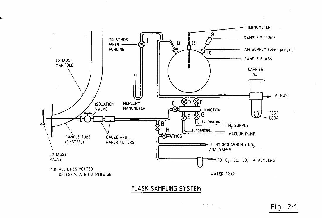
EXHAUST MANIFOLD
TO ATMOS WHEN -PURGING
" _ I MERCURY
SAMPLE TUBE IS/STEEl}
EXHAUST VALVE
N.B. ALL LINES HEA TED
GAUZE AND PAPER FIL TERS
UNLESS STATED OTHERWISE
I
-
1rv'\r"ATMoS
THERMOMETER
SAMPLE SYRINGE
AIR SUPPL Y I",hen purgmg)
SAMPLE FLASK
CARRIER N2 --'- ,
ATMOS
TEST ,,,L _ LOOP
N2 SUPPL Y
VACUUM PUMP
I: TO HYDROCARBON = NOx ANALYSERS
l' rl== TO O2, CO. CO 2 ANALYSERS
WATER TRAP
FLASK SAMPLING SYSTEM
Fi g. 2·1

LEF,'I) :'": :?., :j.~
(ill 2t :-: cl .. n '~J':... ~:~ . E: PK . "in .-: (4. t~!
THf·.:':;H :';-:. (1 AR REJ:..: f1
L! ~:f; Zi..::;;:fi:: ~i .. n.~:.
BASE RUN
RUH:;I· 42£1 HO RUN PEt"1KS. STORED
TYpICAL GAS •
CHROMATOGRAM
(EXHAUST SAMPLE)
[l!L
LU~U .-
?:TT c"" , un 'T' .. ," Pt< tdO .. ';Hf~~;H -;<R ~E.J =
~1
.)
(~
i «
(1 ,
f,
.~1j
ENGINE FUELLED WITH ISO-PENTANE
~~~ BASE FUEL
~==~====:::::::r<, ~;"
~ INTERNAL STANDARD
c'. )~
. ( HEXANE )
RUN i ;,121 DEU&4/.8'.)
AR£fl% KT ARH: TiP£!
',_6.79 197«B -,po, ··_'1.86 1456B ~'Il -Ull 76a7 BII
Lel; 4212 w I <,' .~. 157 pp
-1.29 c:@434l" pr, "
<,.09 5435 pp - 2.27 451300i.! PE:
2.71J 23321 BB -3.93 163ft4 po
-"
TOTAL m;:EA= ·180:?.f"3U i'lIJL f He1 OR= L O!o:etI1E +f!!l
AR.iffT O,t<29 €1. fl3e e.~34 \UH6 ~L ~1l9 O. 9~·7 et. (1(.5 e.~iS6 9.993 H. 1 ::)(1
IG'S8'('&
,AREP."'1. . t<.418 £1.303 6.158 f'. (138 e.!'i03 4.264 t1. i13
9:3.947 ~.49S £1.215
Fig. 2·2

"I ~'i ! :~~ :-\l: :.~~;"i
, tl!( C:if'!;I:l ': Y
/!',J~:~I 1:;"'1.;,
LALltH~AllUN
CHROMATOGRAM
'L ., .n. ·eo C -~·f}'6 ';:=======~-H9
2,,11
'. '" I ,)~ ~ INTERNAL
STANDARD (HEXANEl t'::====== 3,(69
t-
c· • ','!
BASE RUN
RUH if j ~::3
AREI':: R-r
methan~Ij.71 prop ane- 'IU~9
0.89 . butane '0.96 iso.-Ken ane-l.19
hexane . 2.11 2.51
i so -octane 3.69
;:RHl 1 "ff'E :; i!37 Hie SF'H
1 . .::JJ78U0? '}Ha 4~!'9~) Tf:B
, . ~4e9E+07 SH3 1 .:'-627E"'(l7 'f!)B
(939234311) PS ,3f:49i BH
on . "
HO RUN F'Er::~~-: ~;T(I~~[r1 TO. f"iL Ar~E .. ~= (;.? 199£ +fO ~UL <" P'CT(lR~ 1. 3(lIj(1E +,,8
(~F.~/lrr
H.027 (i . {13·~
~~. ft23 9.134:< 0.954 {1 .• )85 (l.(l74
O.lGli
HRtJ)~:
:> . f·33 l.S:444 ';Ulf.0
19.955 29.27B n.S4.J tl f~!:>;}
22./63
Fig. 2·3
CHAPTER 3
EXPERIMENTAL ACCURACY AND IDENTIFICATION OF HYDROCARBONS -DISCUSSION

CHAPTER 3
EXPERIMENTAL ACCURACY AND IDENTIFICATION OF
HYDROCARBONS - DISCUSSION
3.1 Experi mental Accu racy
3.1.1 General Note
During both calibration and engine sampling it was important to keep
liquid additions to the flask to a minimum not only to give
comparable concentrations to those in an engine sample but to
maintain a homogeneous mixture both within the flask and the test
loop, Figure(2.1). That is the flask mixture was assumed to be of
identical component concentration as a sample in the chromatographic
test loop. This assumption was not unreasonable since sample area
cou nt rat i os f or the ba se fu e 1 component we re to with in 1 pe rcent
for a given flask mixture. Both Fleming[17] and Daniel and
Wentworth[4] emphasise the importance of dilution and thorough mixing
of the exhaust sample before any measurements are taken if serious
error is to be avoided. The work in this project has met both these
conditions.
3.1.2 Engine Conditions
Great effort was made to keep air/fuel ratio to within set limits
from one test to another. However this was difficult for coolant
temperatures above 185 degrees F. Generally ai r/fuel ratio was kept
to within about 0.2 of an air/fuel ratio for a given set of engine
tests. Inlet manifold air temperature was maintained to within 1/2
degree C so did not constitute a serious source of error. An effort
was made to keep airflow approximately the same for each test,
differences not amount i ng to more than 5 percent. To avoid excess i ve
residual gas dilution of the intake mixture and subsequent spurious
35

effects on hydrocarbon emissions, a normal consequence of four-stroke
cycle engine operation at high intake manifold depressions[4][30],
the intake manifold depression on the Ricardo engine was maintained
at a low value of about 4 in.Hg for all engine tests. Coolant and oil
temperatures, monitored by thermocouple, were kept to within 2
percent of the planned values by means of a feedback loop system.
3.1.3 Hydrocarbon Mass Calculation
(by the Weighing Method)
The method of weighing'liquid samples in order to obtain their mass
maybe justified by the following argument. Since it was required that
small quantities of liquid samples must be added to the flask to stay
withi n other constraints it was found that samples of around 50 mg
could be weighed to within 1/2 mg on a microbalance which is to
within 1 percent. However evaluation of mass of this magnitude by the
partial pressure method proved to be very innacurate even when using
an inclined water manometer. This was due to small temperature
changes within the flask producing pressure fluctuations of about 50
percent of the partial pressure to be measured. Consequently the
weighing method was adopted as the most accurate.
The accuracy of the weighing method was checked quite simply by the
following procedure. A syringe filled with a paraffin hydrocarbon, n
Hexane, and an empty phi al were wei ghed separately. About 50 mg of
the hydrocarbon were transferred from the syringe to the phi al and
both items were weighed once again. The changes in weight of both
items compared to within 1/2 mg. This process was repeated three
times to ensure repeatabil ity of the accuracy. The calibration
mixture of Iso-pentane,n-Hexane and Iso-octane was made up using the
weighing method. An empty bottle was weighed first, a quantity of n
Hexane added, the bottle and its contents weighed again and the
we_ight of n-Hexane added found by subtraction. Similarly quantities
of Iso-pentane and Iso-octane were added to the bottle and their
masses obtai ned. It shoul d be noted that immedi ately after the n-
36

Hexane was added the bottle was sealed with a screw top and rubber
septum. All further additions, and subsequent withdrawals for
calibration analysis, were made through the septum, therefore
preventing any loss of the mixture from the bottle due to
evaporat i on.
It was found by experiment that during calibration tests changes in
relative concentrations of components to internal standard can
seriously effect the relative response factors of those components.
For this reason it was ensured that the relative concentrations of
Iso-pentane and Iso-octane to n-Hexane in the cal ibration mixture was
comparable with that of a typical engine sample.
37

3.2 Identification of Hydrocarbons
Before any measurement of hydrocarbon levels could be made each
hydrocarbon specie of interest had to be identified first.
Since the engine was run on pure fuels(Iso-octane and Iso-pentane) it was not necessary to fractionate the sample as is sometimes done when running on blended fuels[17] tie. in the case of gasoline which has a broad band of hydrocarbons, fractionating allows separation of
species of high molecular weights from those of low molecular weights). Hydrocarbon identification was made by repeatedly running
typical engine samples through the: chromatograph and establishing a
pattern of the various species and their concentrations. In the case of the special fuels tie. Iso-octane and Iso-pentane) the most promi nant peak after the internal standard was the base fuel. According to theory each hydrocarbon will elute from the column at a different time so retention time maybe used as a method of identification of the various components of interest.
For a given flask mixture the base fuel peak was confirmed by adding a small quantity of the fuel hydrocarbon to the flask and then
noting the change to the chromatogram. In both cases identification of the base fuel was made when the peak increased in size in
proportion to the amount added to the flask with no change to any of the other components in the chromatogram. It was established by
comparing chromatograms for the two fuels ( Iso-pentane and Isooctane) that no other peaks or components of appreciable concentration eluted at the same time as the base fuels. This meant that to a good approximation base fuel peak area counts could be
taken to represent the total concentration of the base fuel in the
eXhaust sampl e.
To facilitate better separation of the other species of interest two
38
metre column lengths were used in the chromatograph. Prior to this
0.9 metre length columns were used giving very poor separation of the
1 ighter components (Methane, Ethane, Propane and n-Butane). However
since these components were in considerably lower concentration than
the base fuel identification was more difficult.
The same method as used for the base fuels was adopted to identify
the retention times or positions in the chromatogram of the lighter
components. However it could be argued that these peaks, believed to
represent the 1 i ghter components, were made up of other components
not identified in the chromatogram with similar or identical
retention times. If this was the case then there would have been some
evidence of partial separation when changing from 0.9metre to 2
metre length columns. In fact there was none so it was reasonable to
suppose that the retention times of those peaks of interest did
infact correspond to those components alone and no others.
Since all components present in si gnificant quantities were
identified the method was checked by comparing the sum of the
hydrocarbon specie levels in PPM C from the chromatographic technique
to the total PPM C from the hydrocarbon analyser. After allowing for
the low levels of unidentified hydrocarbons in the chromatographic
analysis the two methods compared to within 5 percent.
39

CHAPTER 4
EXPERI MENTAL EQU I PMENT

CHAPTER 4
EXPERIMENTAL EQUIPMENT
Photographic Plates(4.1),(4.2),(4.3) & (4.4) illustrate: The
Sampling Flask System, Engine with Fuel and Air Intake Systems, The
Control Panel and finally The Gas Analyser and Chromatograph with
Integrator respectively. The general schematic, Figure(4.1), shows
the position of all equipment used in the experiment. The arrows
indicate the direction of flow of fuel, air, exhaust and data through
the system.
4.1 Sampl ing Flask System
The diagrammatic layout of the flask and interconnecting lines are
shown in Figure(2.1). All interconnecting lines were heated to
approximately 150 degrees C unless stated otherwise. The flask, which
sits inside an insulated box - not shown in Figure(2.1), was heated
by an electrical ring oven to about 200 degrees C. Stainless steel
tubing was used throughout to minimise surface reaction effects with
the sample. All pipework and valves, including the flask, coming into
contact with the sample were cleaned thoroughly with Iso-pentane to
remove deposits which may have contaminated the sample during a
chromatographic test. Although inline filters, shown in Figure(2.1),
take out the small particles from the sample before it enters the
flask, deposits still tended to form on the inside of the flask after
about 10 fillings. For this reason the cleaning process was repeated
several times throughout the experimental work in order to keep
contaminant levels to a minimum.
In the ea rly stages of the work a 1/2 1 i tre fl ask was used for the
40

collection of exhaust samples. However it was found that the capacity
was too small to mask engine transient effects on the exhaust
products therefore producing inconsistent results. For this reason a
5 1 itre pyrex flask was finally chosen giving the desired averaging
effect on exhaust composition transients.
It was found that continual changes of pressure and temperature had a
fatigue effect on the flask finally leading to an implosion of the
flask while evacuating the contents. Consequently for future
experiments of this nature a stainless steel flask would be a safer
and more adequate enclosure.
A - I represent shutoff valves - Figure(2.1).
During purging air is admitted to the flask via screw top, position
(1) illustrated in Figure(2.1), and finds its way out via valve I and
the test loop. In this manner both the flask and the test loop were
purged of impurities. Air was used because it is cheaper than
nitrogen and was therefore normally left on overnight to purge the
flask thoroughly of the old sample. Finally the air was flushed out
with nitrogen using the filling and emptying technique already
described[2.2]. The contents of the fl ask were chromatographed to
check for impurities and then evacuated to around 150 mmHg ready to
accept an engine sample.
It is well known that hydrocarbon concentration varies with distance
along the exhaust pipe and also with engine crank angle[4]. The
sample size should therefore be large and its collection as close to
the exhaust valve as possible to mask transient effects. In this
project the exhaust products were sampled about an inch away from
the exhaust valve and passed via a stainless steel tube through a
fine gauze filter and then a 1 micron paper filter. The isolation
valve A was kept closed until the engine had run up to speed which
prevented unwanted products from entering the filters during start
up.
41
When engine conditions were steady and the air/fuel ratio was correct
the sample flow was diverted to the flask via valves C and D until flask pressure had equalled exhaust pressure, usually about 5 mmHg gauge. At this point valves C and D were closed and the sample was left to settle in the flask before adding the internal standard.
When the flask sample was ready for chromatographing, valves D and F were opened allowing a low flowrate of sample through the test loop
to atmosphere. The test loop was then switched into the carrier circuit of the gas ch romatograph and 1 eft for a few seconds in th i s
position to ensure that the loop had been swept clear of the sample. During this short period the sample flow escaped directly to
atmosphere until the test loop valve was switched back refilling the test loop once again ready for the next chromatographic run.
42

4.2 Ai r Intake System
All d i agrammat ic detai I s of the system and a i rfl ow route a re shown in
F i gu re (4.2) •
An Alcock viscous air flow meter with inclined manometer was used for
monitoring the air flow into the engine. The Viscous Flow air meter
contains a Meter Element which is a honeycomb of long, narrow
triangular passages. Within the working range, the flow through these
passages is viscous and the resistance of the element is, therefore,
directly proportional to the velocity. The air enters through a
cleaner and then passes through the meter element, which is made up
of alternate layers of flat and corrugated strip metal wound upon a
core. "Even very irregular flow, as produced by a single cylinder
engine without any smoothing, does not cause significant error.
The air was channelled by means of a flexible hose from the flow
meter to the filter body, Figure(4.2). Since the Viscous Flow air
meter contained a cleaner, the filter element normally housed in the
fi lter body was di spensed with. Th is had the advantage of avoi di ng
an unnecessary pressure drop along the inlet tract. An electric
element housed in the filter assembly was used to heat the air before
it entered the following section of the inlet tract in order to
assist in fuel vaporization.
The throttle was of the butterfly type and control was affected by a
pulley wheel and cable system linked to the throttle spindle. The
cable was connected to an e1ectro-mechanica1 solenoid which was
operated from the control panel according to load and speed demand.
The throttle spindle was sealed with an '0' ring which prevented
unwanted air leaks into the system.
llfe p1en!lm chamber assisted in dampening pressure fluctuations due to
the reciprocating nature of the engine. The chamber also housed a
mercury thermometer, used to monitor air temperature and a
43
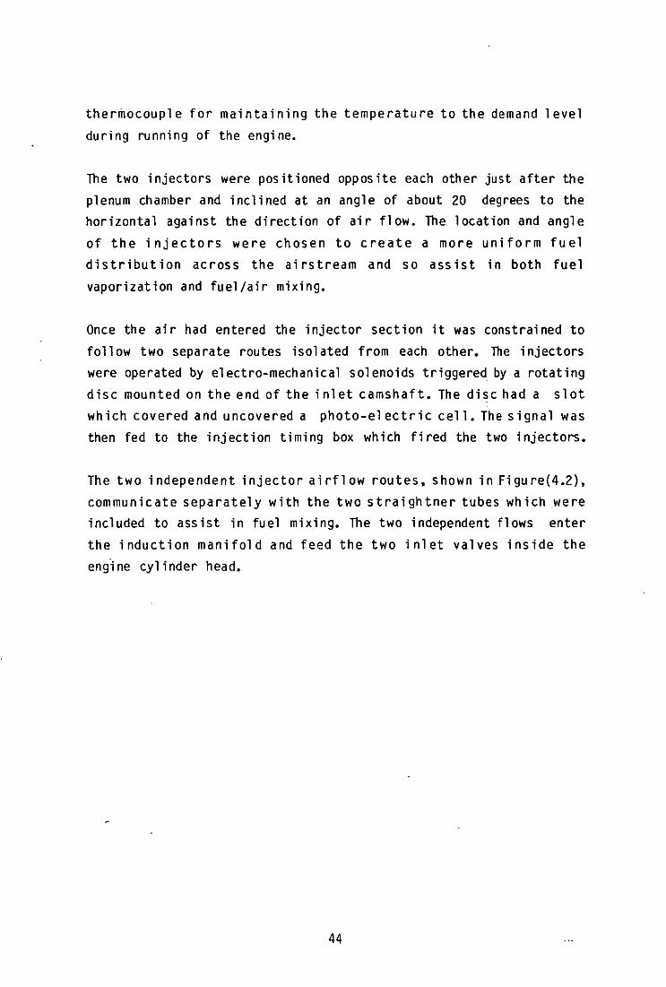
thermocouple for maintaining the temperature to the demand level
during running of the engine.
The two injectors were pos it ioned oppos ite each other just after the
plenum chamber and inclined at an angle of about 20 degrees to the
horizontal against the direction of air flow. The location and angle
of the injectors were chosen to create a more uniform fuel
distribution across the airstream and so assist in both fuel
vaporization and fuel/air mixing.
Once the air had entered the injector section it was constrained to
follow two separate routes isolated from each other. The injectors
were operated by electro-mechanical solenoids triggered by a rotating
disc mounted on the end of the inlet camshaft. The disc had a slot
which covered and uncovered a photo-el ectric cell. The signal was
then fed to the injection timing box which fired the two injectors.
The two independent injector airflow routes, shown in Figure(4.2),
communicate separately with the two straightner tubes which were
included to assist in fuel mixing. The two independent flows enter
the induction manifold and feed the two inlet valves inside the
engi ne cyl i nder head.
44

4.3 Fuel System
The fuel system network, Figure(4.3), was designed with the intention
of using it as a multi-fuel system since it was required that the
engine should be run on three different fuels namely, gasoline, Iso
pentane and Iso-octane. The system was fabricated to meet the engine
requirements and supply the injectors with sufficient fuel at 30 psi.
It was also important that the fuel was free from air and vapour
pockets.
A burette was used for measuring fuel flow and details of the
calculations are given in Appendix(E). A Bosch electric fuel pump
with pressure regulator was used for feeding the fuel under pressure
( 30 psi ) to the injectors.
In the early stages of the work when setting up and commissioning the
engine and equipment it was both convenient and more economical to
run on gasoline rather than a pure hydrocarbon fuel. For this reason
the system was designed to cater for the use of gasoline as well as
the special fuels.
The schematic in Figure(4.3) is fairly self explanatory but will be
discussed briefly. When the engine was to be run on gasoline stop
cock B was closed to isolate the special fuels tank from the system
and breather C was then opened to allow trapped air to escape as the
system was being filled with the fuel. Stop cock A was opened
allowing the filtered fuel to fill the system. Fuel was then fed
under pressure to the injectors by means of a Bosch electric fuel
pump. The pump del i vered a constant flow at a gi ven pressu re, the
excess fuel bei ng fed back to the suct ion side of the pump vi a the
pressure. relief valve also used to set the fuel pressure of 30 psi. A
pressure gauge monitored the fuel pressure.
45

When changing over to run the engine on either of the special fuels
stop cock A was closed and the residual gasoline remaining in the
system was drained via plug C. Breather C was then closed and stop
cock B was opened to allow the new fuel to fill the system. Normally
the engine was run for a few minutes on the new fuel before changing
the oil for a fresh set of tests. This allowed the old fuel to be
flushed out of the system completely.
When running on Iso-pentane the fuel pump was semi immersed in a
refridgerated water bath to prevent fuel vapour forming in the
suction line leading to vapour lock and subsequent overheating of the
pump.
46

4.4 Gas Chromatograph(G.C.)
A pye Unicam series 104 gas chromatograph was used in the
experi ments.
The G.C. was fitted with dual heated flame ionisation detectors(FIDS)
and dual columns. The dual column system compensates for effects due
to small changes in the chromatographic condition so that both
columns are affected similarly. The unit was equipped with an
ionization amplifier, a detector oven controller and an oven
programmer. A mixture of hydrogen and air was used for the FID flame
and nitrogen was used as the carrier gas. The object of a G.C. is to
separate the various components of a given sample, quantitatively.
The columns perform the function of separation with subsequent
detect i on and measu rement by the FID's and anc ill i ary equi pment.
The sample was carried from the test loop and through the column by
the carrier gas. The components in the sample were separated
according to their boiling points, the lighter hydrocarbons eluting
from the column first. The FID's operate on the principle that the
electrical conductivity of a gas is directly proportional to the
concentration of charged particles within the gas. The sample
component contained in the effluent gas from the column is mixed with
hydrogen and burned in air. As the sample enters the flame a
percentage of the molecules are ionized forming positive and negative
ions and free electrons. The extent of the ionization depends on the
nature of the compound and the temperature of the flame (dependent on
the ratio of hydrogen/air/carrier gas).
The sampl e is passed through one of the columns and it is the
difference in levels of ions between the two columns that is
measu.red. These ions give rise to a voltage which is ampl ified by the
ionization amplifier and then fed to the integrator for further data
handl ing. For chromatographic conditions see Appendix(B).
47
4.5 Electronic Integrator
The Hewlett Packard integrator is responsible for turning voltage
1 eve 1 s fed from the chromatograph into area counts correspondi ng to
PPM C levels. A fast sampling method was used to transform the
voltage levels into area counts which were finally produced in a
graphical plot against time. The various peaks which appear in the
plot or chromatogram quantitatively represent components of the
chromatographed sample as shown in Figures(2.2) & (2.3). The
retention time of each peak appears in the chromatogram indicating
the relative elution times of the components making up the sample.
Finally a table is printed out indicating retention times, area
counts and other relevent details for each component appearing in the
chromatogram.
Before a sample is passed th rough the ch romatograph the controll i ng
parameters for the integrator need to be entered which are the
foll owing
(a) Zero - The integrator base zero level
control potentiometer on the amplifier of the
is set by means of a \
chromatograph. This in
effect adjusts for any slight differences in base voltage levels
between the two FID's. It also allows setting of the plot baseline to
any position between the left margin (-6) and the right margin (lOO).
The value entered is a set percentage of full scale. In the sample
analysis it was found that the default value of zero was convenient
which sets the plot baseline approximately 1.3 cm. from the left edge
of the paper.
(b) Attenuation (ATT) - This level is set from the integrator to
ensure that peaks appearing in the chromatogram remain within scale.
It sets the maximum signal voltage at full-scale deflection on the
recording paper. However the area count is totally independent of
attenuation changes on the integrator. The signal voltage level to
48
the integrator, which must not exceed it's range of 1 volt, is
attenuated appropriately on the ionisation amplifier of the
chromatograph. For the analysis attenuation was set to ensure that
the peaks appeared clearly in the chromatogram and during
measurement was set to a value of 4 which corresponds to a maximum
signal voltage at full scale deflection of 16 mv.
(c) Chart speed (CHT SP) - This controls paper advance speed in
cm./min, helping visual identification of the various peaks. A value
is chosen to give the clearest chromatogram (for the analysis a value
of 2 was chosen).
(d) Peak width (PK WD) - This controls selectivity in distinguishing
peaks from noise or each other by filtering data sufficiently to
improve the apparant signal-to-noise ratio. Successful use of PK WD
requires just enough filtering to eliminate noise from being
interpreted as peaks, but not enough to distort chromatographic
i nformat i on. The value used, 0.01, was obtai ned by measu rement of the
time width (in minutes) at half-height of the narrowest (fastest)
peaks of interest. Therefore peaks having values less than this
figure were ignored.
(e) Thresh-hold (THRSH) THRSH's function is to remove from the
signal any information the integrator should not consider
significant. A reasonable choice for THRSH (one insuring adequate
peak detection without too much sensitivity to noise or trace
impurities) is a value between the auto-THRSH (value determined by
the integrator from the signal), and the value used for ATT that
plots the smallest peaks of interest so as to be at least 1 mm. in
height, as measured from their starting points. If the auto-THRSH
value itself is used, some noise may be mistaken for peaks. The value
for THRSH chosen in the analysis varied from 0 to 2 (ie. 1mv - 4mv)
depending on the type .of chromatographic run (ie. baseline run,
calibration or exhaust sample run).
(f) Area rejection (AR REJ) - Peaks with areas less than the value
49

for AR REJ. are discarded. Values represent area counts (1 area count
= 0.125 microvolts.- sec.). In the analysis no area rejection was necessary and the default value of zero was used.
Typical experimental values for the above parameters are given in Figures(2.2) & (2.3). When all input parameters had been entered the
integrator was put into start mode and at the same instant the test loop valve was switched from fill to inject. When all peaks of
interest had emerged the integrator was put into stop mode and a chromatographic table was printed out. The integrator was then re
zeroed ready for the next sample.
50

4.6 Exhaust Gas Analyser
The system is designed to sample and measure the concentrations of
carbon monoxide, carbon dioxide, oxygen, NOX and hydrocarbons in
engine exhaust and includes filters, a heated sample line with
proportional temperature control, a cooling unit and pumps. The CO,
C02 and 02 analysers are supplied by a sampling system which passes
the gas through a cooler unit. The hydrocarbon and the NOX analysers
are supplied by a heated sampling system and are completely separate
and independent apart from their zero grade and span gas supplies.
The five analysers incorporated in this system are discussed briefly:
(a) Carbon monoxide and carbon dioxide analysers are of the infra-red
type manufactured by The Analytical Development Company Limited.
Measurement uses an infra-red absorbing technique and the analyser is
a non-dispersive double beam unit in which the gas to be measured is
passed through an optical cell, either continuously or as a static
sample. The gas is not affected by the measurement and may be
recovered if desired. The analyser output meter is calibrated in
terms of gas concentration, but this type of instrument operates as a
comparator: the cal ibration is not absolute, but is establ ished by
standardising with a known gas mixture at one point on the calibrated
scale. The unit is zeroed using clean air. The infra-red detector is
of the Luft-type which receives low energy infra-red radiation from a
simple hot wire source in the analyser, but, because it is filled
with a pure sample of the type of gas to be measured, can respond
only to energy in that region of the infra-red spectrum corresponding
to the absorption band peculiar to that gas. When the gas to be
measu red enters the analyser it passes through a cell in the path
between the radiating source and the detector and, according to the
cohcentration present, absorbs some radiation and thus reduces the
level of energy reaching the detector. It is this change of energy
which is amplified to give the analyser output signal.
51

The infra-red radiation source consists of a heated wire in a quartz
tube mounted in the source block, which is located at the opposite
end of the optical bench to the detector. Radiation from the source
is reflected within the mounting block and passes out of a
symmetrical pair of rectangular apertures into the analysis tube set.
This comprises of a pair of tubes which are internally highly
polished and gold plated to ensure high transmission of radiation
into the detector cells. One tube is used for the gas to be measured,
whilst the opposite tube is used for reference, and is usually filled
with dry air. The sample cell may be divided by windows into various
lengths, to give different ranges of sensitivity, the unused sample
cells generally being flushed with a non infra-red absorbing gas such
as oxygen or nitrogen, or gas free of the component being measured,
for example, fresh air for carbon monoxide analysers.
(b) NOX analyser ( BOC special gases) - The heart of the Luminox 20
IB chemiluminescent analyser is the chemiluminescent gas phase
reaction between ozone and nitric oxide. The reaction produces light
measured by a photomultiplier tube and is proportional to the nitric
oxide concentration. The Luminox 201B operates at low pressure in
order to maximise the light output from the chemiluminescent reaction
and allows wet sample gas to be analysed without the need to maintain
the entire pipework system at 70 degrees C or more. Calibration is
again performed by standardising with a known gas mixture.
(c) Hydrocarbon analyser (Analysis Automation Limited model 523 )
detects and measures hydrocarbons utilising a flame ionization
detector (FID). A small, continuous flow of sample gas is burnt in a
polarised hydrogen flame. During the combustion process compounds
containing carbon - hydrogen bonds form ions; a potential is applied
between the flame and a collector electrode causing migration of the
ions to the electrode. The resulting ion current is related to the
concentrat i on of hydrocarbon in the sample. Th i s si gna 1 is amp 1 ifi ed
and displayed by the electronics module of the analyser. Calibration
is by a standard propane/ai r mixture. On start up the unit needs to
52

----- -----------
be left for about half an hour to allow the oven to reach its set
temperature about 150 degrees C. When the flame is 1 it the unit is
left for a further half hour to allow stabilisation of the FID base
level. The analyser is then zeroed and calibrated before commencing
measurement of a sample.
53

4.8 Injection System
Injection of the fuel was electronically actuated by solenoid valves
housed in each of the two injectors. The solenoids were fired from a
manual fuel injection unit which was fed with cam pulses and a 12
volt supply. The quantity of fuel injected was controlled manually by
a potentiometer mounted on the injection unit. Injection occurred at
half engine speed or every time a cam pulse was fed to the injection
uni t •
55

4.7 Ignition System
A lumenition and coil combination were used to generate a spark at the plug. Engine position was monitored by photoelectric cells triggering on TOC and 2 degree slots cut into a disc bolted to the
flywheel. A photoelectric cell which picked up on a slot machined in
another disc, fixed to the inlet camshaft, indicated the position in the engine cycle. The TOC, 2 degree and cam slot pulses were fed to a timing box which allowed timing adjustment in increments of 2 degrees BTOC us i ng a thumb whee 1. When engi ne pos it i on corresponded to the thumb wheel setting on the timing box the lumenition was switched on, which in turn switched off the coil producing a spark at
the plug.
54

PLATE 4.1 FLASK SAMPLING SYSTEM (FLASK INSIDE BOX)

PLATE 4.2 ENGINE WITH ANCILLARY EQUIPMENT

•
•
,
PLATE 4.3
•
•
I' ~ 'I' . I!....~
•••• •••• • •
(ONTROl PANEL
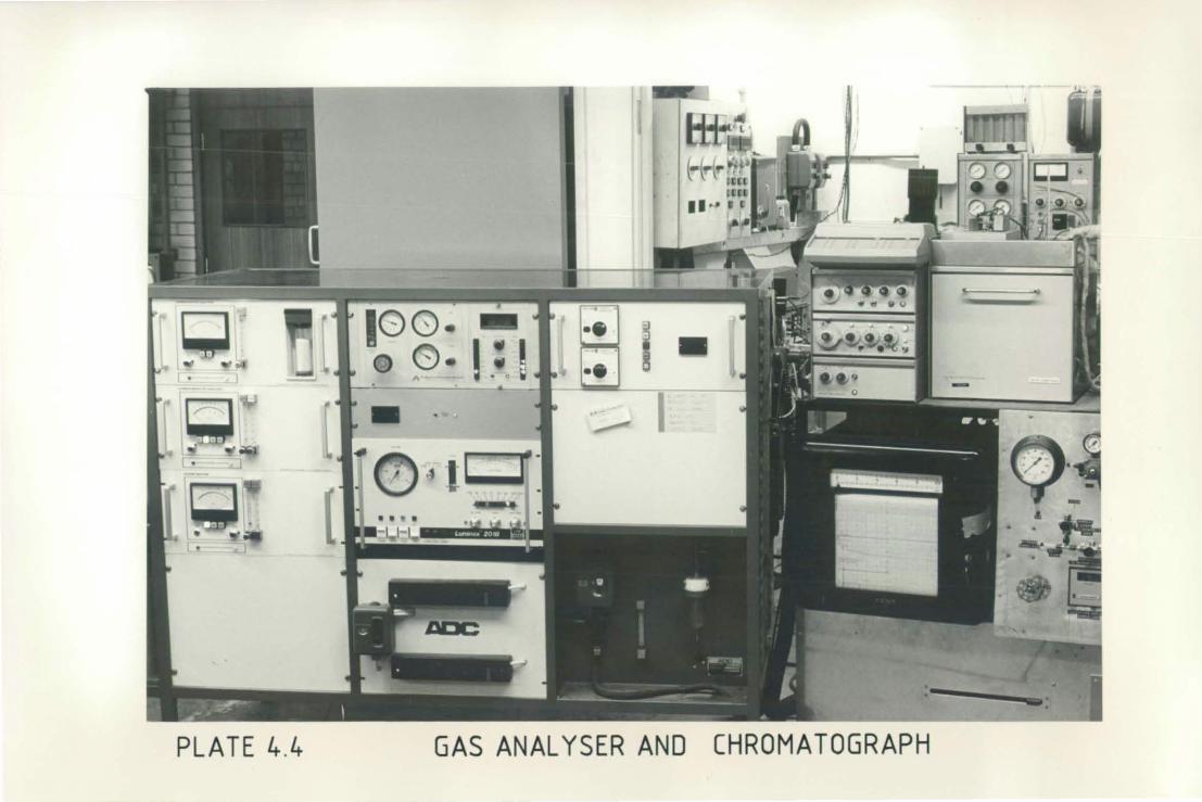
.' --
PLATE 4.4 GAS ANALYSER AND CHROMATOGRAPH

FUEL SYSTE
AIR IN
M [= . -
1111 ,....... VISCOUS
DYNOMOMETER
TO 11 INjECTORS If
I AIR HEATER
f-- ENGINE f---f
L_
r-- --,..-,....
FLOW METER
1111 1 2 3 .4 5 6 7
I CONTROL PANEL
ULSE ULSE I ANGLE PULSE MAIN PANEL
1. CAM P 2. TOC P 3. CRANK 4. THERM o COUPLES 5. IGNITIO N DRIVE 6. INJECT OR. DRIVE 7. THROT TLE CONTROL
GENERAL SCHEMATIC
MICRO COMPUTER
EXHAUST ! I DATA
SAMPLE - FLASK CHROMATOGRAPH r-• SYSTEM - AND
INTEGRATOR
I -
I GAS ANAL YSER
Fig. 4·1

ALCOCK VISCOUS FLOW METER
FLEXIBLE PIPE
AIR 1Nl AKE SYSTEM
MANOMETER
AIR HEATER
- -------Hf--THROTTLE
, ... _ ......... _,
PLENUM
[
THERMOMETER J AND THERMOCOUPLE
.......... '1..-. , .... ---INJECTOR
J--t-l_-STRAIGHTNER TUBES
I \ '- ----
------
1Nl f. T MANIFOL 0
• INLE T VAL VES --
Fig. 4·2

GASOLINE TANK A
FIL TER
STOP VALVE A
DRAIN PLUG "C"
SURETTE
TANK S -{ISO - oCr ANE ]. ISO - PENTANE
STOP VAL VE "S"
SREA THER "C"
PRESSURE REGULATOR
TO INJECTORS
FUEL SYSTEM
PRESSURE GAUGE (30 psi)
FEED LINE
SUCTION LINE
FUEL PUMP (SOSCH)
REFRIDGERA HO BATH
Fig. 4·3

CHAPTER 5
GENERAL DISCUSSION OF RESULTS AND CONCLUSIONS
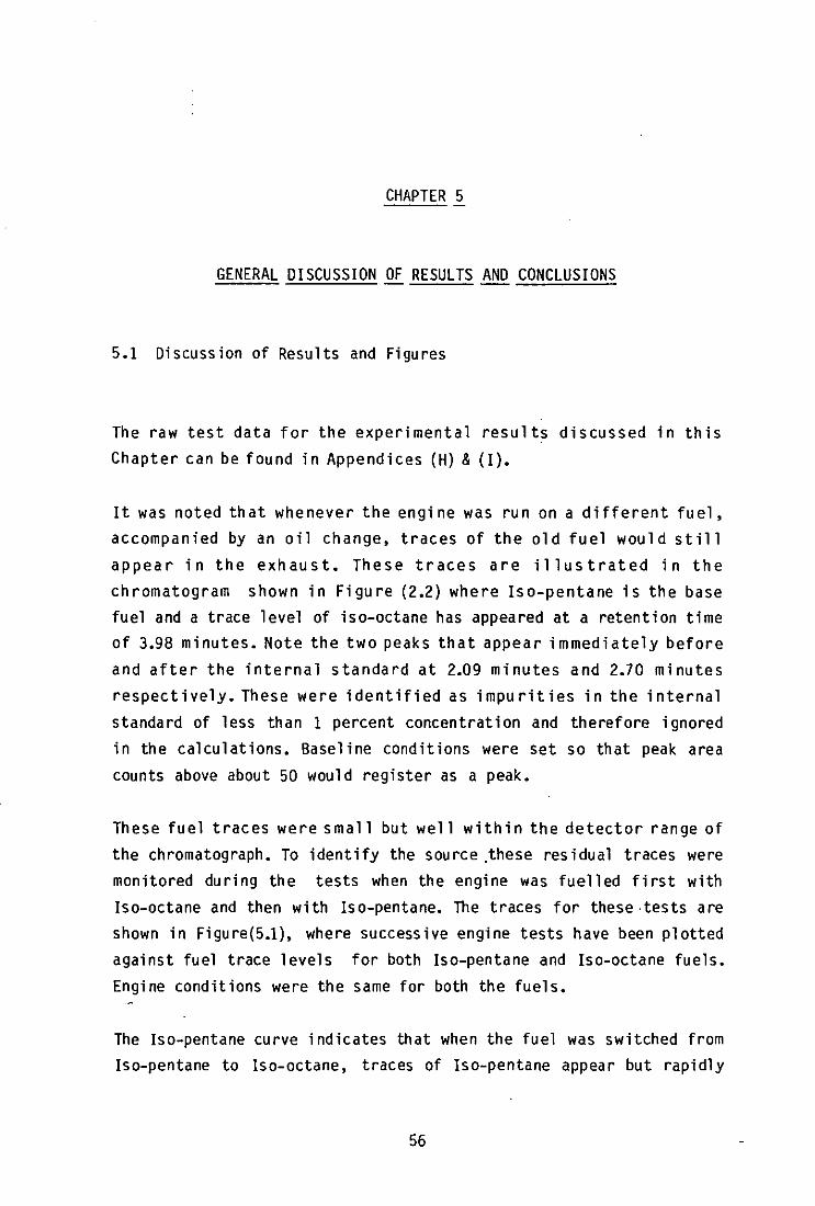
CHAPTER 5
GENERAL DISCUSSION OF RESULTS AND CONCLUSIONS - --
5.1 Discussion of Results and Figures
The raw test data for the experimental results discussed in this
Chapter can be found in Appendices (H) & (I).
It was noted that whenever the engi ne was run on a different fuel,
accompanied by an oil change, traces of the old fuel would still
appear in the exhaust. These traces are illustrated in the
chromatogram shown in Figure (2.2) where Iso-pentane is the base
fuel and a trace level of iso-octane has appeared at a retention time
of 3.98 minutes. Note the two peaks that appear immediately before
and after the internal standard at 2.09 minutes and 2.70 mi nutes
respectively. These were identified as impurities in the internal
standard of less than 1 percent concentration and therefore ignored
in the calculations. Baseline conditions were set so that peak area
counts above about 50 would register as a peak.
These fuel traces were small but well within the detector range of
the chromatograph. To identify the source ,these residual traces were
monitored during the tests when the engine was fuelled first with
Iso-octane and then with Iso-pentane. The traces for these ·tests are
shown in Figure(5.1), where successive engine tests have been plotted
against fuel trace levels for both Iso-pentane and Iso-octane fuels.
Engine conditions were the same for both the fuels.
The Iso-pentane curve indicates that when the fuel was switched from
Iso-pentane to Iso-octane, traces of Iso-pentane appear but rapidly
56

decrease to zero as the number of engine tests increase. On the other
hand the Iso-octane curve indicates greater traces which decrease
more slowly than those for the Iso-pentane. This suggests that the
traces of the old fuel were infact present in the engine oil and not
in the test fuel. If these traces had been present in the test fuel
then a constant hydrocarbon trace level would have been expected
throughout the tests but clearly this is not the case. For the first
test the concentration of Iso-pentane is about 5 percent of that of
Iso-octane when running on Iso-octane and Iso-pentane fuels
respectively. Again this demonstrates the higher solubil ity of Iso
octane in oil than Iso-pentane, and suggests that each fuel trace is
being gradually desorbed out of the oil as the number of tests
increase for a given fuel. The results of Figure (5.1) illustrate the
desorption part of the mechanism well.
Mathematical models [10],[13] and experimental results [24],[11],[14]
have shown that hydrocarbon levels decrease with increasing coolant
temperature. Theory suggests that an increase in wall temperature is
accompanied by a thinner cylinder wall oil film and a higher Henry
Constant for the oil. This leads to lower fuel/oil absorption rates
and therefore lower hydrocarbon 1 eve 1 s. Th i s trend cons i stent with
Figure(5.2) (speed 2000 RPM and load 19 NM) indicates a 20 percent
difference in base fuel hydrocarbon levels for Iso-octane and Iso
pentane fuels emphasising the effect of iso-octane's higher fuel/oil
solubility. However this difference is not entirely due to the
absorption/desorption mechanism. The importance of trapped volumes as
a hydrocarbon source has been stressed in other studies[13],[2]. It
has been shown that base fuel hydrocarbon levels produced as a result
of trapped volumes are about 10 percent greater for Iso-octane than
for Iso-pentane fuel for the same engine conditions. A derivation of
this is given in Appendix (G). It follows that any
absorption/desorption effect should show up on top of this 10
percent. Therefore assuming other sources such as surface deposits to
contribute equal amounts of hydrocarbons for both fuels, Figure
(5.2), only a 10 percent difference in base fuel hydrocarbon levels
could be attributed to the absorption/desorption effect.
57
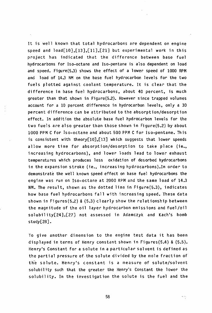
It is well known that total hydrocarbons are dependent on engine
speed and 10ad[10],[13],[1l],[21] but experimental work in this
project has indicated that the difference between base fuel
hydrocarbons for Iso-octane and Iso-pentane is also dependent on load
and speed. Figure(5.3) shows the effect of a lower speed of 1000 RPM
and load of 14.3 NM on the base fuel hydrocarbon levels for the two
fuels plotted against coolant temperature. It is clear that the
difference in base fuel hydrocarbons, about 40 percent, is much
greater than that shown in Figure(5.2). However since trapped volumes
account for a 10 percent difference in hydrocarbon levels, only a 30
percent difference can be attributed to the absorption/desorption
effect. In addition the absolute base fuel hydrocarbon levels for the
two fuels are also greater than those shown in Figure(5.2) by about
1000 PPM C for Iso-octane and about 500 PPM C for iso-pentane. This
is consistent with theory[10],[13] which suggests that lower speeds
allow more time for absorption/desorption to take place (ie.,
increasing hydrocarbons), and lower loads lead to lower exhaust
temperatures which produces less oxidation of desorbed hydrocarbons
in the expansion stroke (ie., increasing hydrocarbons).In order to
demonstrate the well known speed effect on base fuel hydrocarbons the
engi ne was run on Iso-octane at 2000 RPM and the same load of 14.3
NM. The result, shown as the dotted line in Figure(5.3), indicates
how base fuel hydrocarbons fall with increasing speed. These data
shown in Figures(5.2) & (5.3) clearly show the relationship between
the magnitude of the oil layer hydrocarbon emissions and fuel/oil
solubil ity[24],[27] not assessed in Adamczyk and Kach's bomb
study[28] •
To give another dimension to the engine test data it has been
displayed in terms of Henry constant shown in Figures(5.4) & (5.5).
Henry's Constant for a solute in a particular solvent is defined as
the partial pressure of·the solute divided by the mole fraction of
th'e solute. Henry's constant is a measure of solute/solvent
solubil ity such that the greater the Henry's Constant the lower the
solubility. In the investigation the solute is the fuel and the
58

solvent is the engine oil. Since no literature on the Henry
Constants of Iso-pentane and Iso-octane in the engi ne test oi 1 was
available, an experiment using a chromatographic technique, was
carried out, Appendix(H), to determine the Henry Constants of Iso
pentane, n-Hexane and Iso-octane in the engine test oil for various
coolant temperatures. The results shown in Figure(H.5), illustrate
that for a temperature of 350 degrees K Iso-octane is about 8 times
as soluble in the engine oil as Iso-pentane. It should be noted that
as Henry Constant increases fuel/oil solubility falls. In Figure
(5.4) the range of engi ne coolant temperatu res have been di sp 1 ayed in
terms of reciprocal of Henry constant for both the fuels on a common
data line. The results illustrate both the higher solubility of Iso
octane in oil than Iso-pentane for the same coolant temperature and
the consequent effect of fuel/oil solubility on base fuel hydrocarbon
emi ss ions.
A similar but steeper trend is shown in Figure (5.5) for a lighter
speed and load combination. The Henry Constants for both fuels are
unchanged to those of Figure (5.4) but the lower speed gives more
time for fuel/oil absorption and the lighter load leads to lower
exhaust temperatures which produces less oxidation of desorbed
hydrocarbons in the expansion stroke. The combined result of lower
speed and lighter load has increased base fuel hydrocarbons for Iso
octane by about 1000 PPM C and Iso-pentane by about 500 PPM C with
other engine conditions essentially constant.
Although it has been assumed that deposits would not contribute
significantly to the base fuel hydrocarbon levels it is quite
possible that they may have had an irregular effect on the results.
Wentworth[18] proved that deposit location has considerable influence
on the contribution of deposits to exhaust hydrocarbon concentration.
Experimental evidence[18] showed that deposits placed at specific
pOints on the surfaces of the combustion chamber and piston crown
produced. increases in hydrocarbons of the order of 100 PPM C. It was
found that deposits in the vicinity of the exhaust valve produced
greater hydrocarbon increases than for any other location in the
59

combustion chamber. However if the deposits were to cover the entire
combustion chamber, as in a running engine, the hydrocarbon levels
due to deposits could be much higher. The deposits could be
responsible for an irregular effect on the base fuel hydrocarbons
producing a scatter on the results. This could be a feasible
explanation for much of the scatter present in the engine test data -
Appendix(I) •
Shinn and 01son[31], investigating factors affecting unburned
hydrocarbons, were forced to abandon early experiments with a CFR
engine due to poor repeatability which was attributed to cyclic
vari at ions of the engi ne. Although the authors of the paper[31] were
aware of the presence and formation of chamber deposits due to
condensation of fuel vapour on the walls the effects of these
depos its on exhau st hyd rocarbons was not real i sed. However in th i s
project deposit formation was minimised by motoring the engine until
warm before carrying out an engine test. This prevented the
condensation of fuel on cold wall surfaces which would lead to higher
wall depos its. It has been assumed that whatever depos its may
contribute to hydrocarbon emissions, on average they contribute equal
amounts to the base fuel hydrocarbon levels for the two fuels. It is
also possible that the position of the top piston cylinder ring gap,
believed to be a controll ing factor in hydrocarbon emissions[15],
could have affected the scatter in the data - Appendix(I). Further
details of this effect may be found in the literature survey -
Chapter[l] •
The Oent & Lakshminarayanan[lO] model has predicted that about 50
percent of total hydrocarbons in the exhaust are due to the
absorption/desorption effect (n-Octane as the fuel). Experiment has
shown about 30 percent due to this mechanism but it has only
considered the absorption/desorption effect in terms of the
difference shown between the two levels of base fuel hydrocarbons for
Is'o-octane and Iso-pentane. This does not represent the total
isolated effect of the mechanism on exhaust hydrocarbons for either
Iso-octane or Iso-pentane fuel. For instance if Iso-pentane was
60
replaced by a fuel with very low solubility in oil (ie. Propane)
any difference in base fuel hydrocarbons between this fuel and Iso
octane (less unequal contributions from other sources such as trapped
volumes) would essentially represent the entire absorption/desorption
contribution for Iso-octane. A fuel such as Propane would be a good
choice since it produces comparatively low increases in exhaust
hydrocarbons due to oil layers in the cylinder of a spark ignition
engine [23]. Consequently the absorption/desorption effect on
hydrocarbon emissions could be even more Significant than found in
this work.' In addition to this the model has several limitations
which could also help to account for the discrepancy. Firstly the
model assumes a uniform oil film thickness on the cylinder
surface[22] and secondly the Henry Constant for the fuel/oil
combination was estimated from extrapolation of data (known to be
prone to error) given by Chappelow & Prausnitz[25].
Consequently considering the limitations of both the model and
experiment, the presented results compare favourably with those
predicted by the model.
61

5.2 Conclusions
The differing effect of conditions inside the engine for the two fuels was not investigated in detail since it was assumed that surface deposits, quench layers etc. made an equal contribution to
the hydrocarbon emissions for both fuels. However a brief
mathematical analysis, Appendix(G), has shown that hydrocarbon levels
produced as a result of crevice volumes are about 10 percent greater for Iso-octane than for Iso-pentane fuel for the same engine conditions. Therefore any absorption/desorption effect must appear on top of this 10 percent difference.
Since the object of the experiment was to assess the significance of the absorption/desorption effect in a running engine surface deposits would therefore be encountered. The differing effect of these surface
deposits on exhaust hydrocarbons for the two fuels has not been assessed experimentally. However experimental evidence [18] suggests that deposit formation upon the surfaces of both the cylinder head
and piston crown, especially in the vicinity of the exhaust valve, can increase hydrocarbon emissions in the exhaust. It was found that
increases of about 200 PPM C would not be uncommon from an engine having surface deposits. However it is difficult to say how hydrocarbon species would be affected by deposit formation within the
Ricardo engine. It may be concluded that there was some increase in base fuel hydrocarbons due to surface deposits within the combustion chamber for the two fuels Iso-octane and Iso-pentane. It is probable that surface deposits could have had an irregular effect on hydrocarbon emissions accounting for the highly scattered data. However it is assumed that the difference between base fuel
hydrocarbon emissions due to surface deposits for the two fuels is not significant.
Since quench layers are closely controlled by molecular diffusion effects and these depend on molecular weights, there would have been
62

a difference in hydrocarbon contributions for the two fuels, Iso
octane and Iso-pentane, due to this source. However since quench
layer sources are considered to be small[l),[2],[9],[3] compared to
other sources such as ring crevices, absorption/desorption and
deposits their contribution to the difference in hydrocarbon levels
for the two fuels would be insignificant. Therefore, apart from the
10 percent due to crevice volumes, any difference in base fuel
hydrocarbon levels between the two fuels has been attributed to the
absorption/desorption mechanism. This was not unreasonable in the
light of the fact that hydrocarbon sources such as those already
mentioned were thought to remain fairly unchanged for all the
experiments and therefore to make the same sort of contribution
towards hydrocarbon emissions for the two fuels. The only parameter
to have been.significantly changed was engine coolant temperature, in
order to show the temperature dependence of the fuel solubility
effect in the oil.
The data indicate a small difference in hydrocarbon levels for the
two fuels, about 400 PPM C at 2000 RPM( varies according to coolant
temperature), Figure(5.2), for fixed engine conditions but half of
this difference (200 PPM C) is due to crevice volumes. Consequently
only 200 PPM C ·can be attributed to the absorption/desorption
mechanism. However this effect is shown more markedly, about a 900
PPM C difference in base fuel hydrocarbons, Figure(5.3), when
running at 1000 RPM and a comparatively light load of 14.3 NM. In
contrast to the 50 percent indicated in the model[lO] experiment has
shown that about 30 percent of total hydrocarbons in the exhaust are
due to the absorption/desorption mechanism. Two reasons are suggested
for the 20 percent discrepancy. Fi rstly experiment has not assessed
the total effect of absorption/desorption on exhaust hydrocarbons and
secondly the model makes certain assumptions which could have
exaggerated the predicted absorption/desorption effect on hydrocarbon
emissions.
The absorption/desorption mechanism has been shown to be a
63

significant sourc·e of hydrocarbons for higher molecular weight fuels,
such as Iso-octane and therefore gasoline. Further work could be
addressed to synthetic fuel blends and their combined effect with
alternative engine oils.
It should be noted that only those hydrocarbon species making a
significant contribution were identified and measured. In the future
it may become necessary to consider how low hydrocarbon
concentrations (about 50 PPM Cl are affected by the
absorption/desorption mechanism.
64
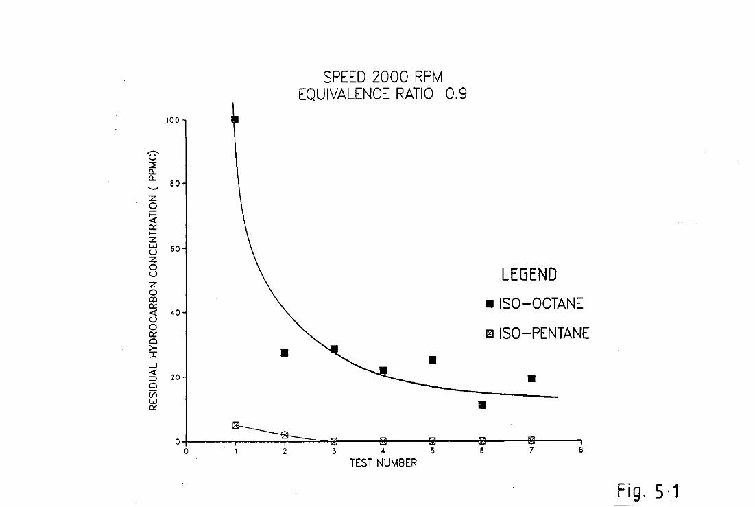
100
.-.. u ~ a.. a..
60 '-" Z 0
~ 0:: f-Z W 60 U Z 0 U Z 0 CO 0:: -er 40 U 0 0:: Cl >-::c ...J -er 20 :::> Cl Vl W 0::
0 0 2
SPEED 2000 RPM EQUIVALENCE RATIO 0.9
•
345
TEST NUMBER
• 6
LEGEND
• ISO-OCTANE
I8l ISO-PENTANE
•
7 6
Fig. 5·1
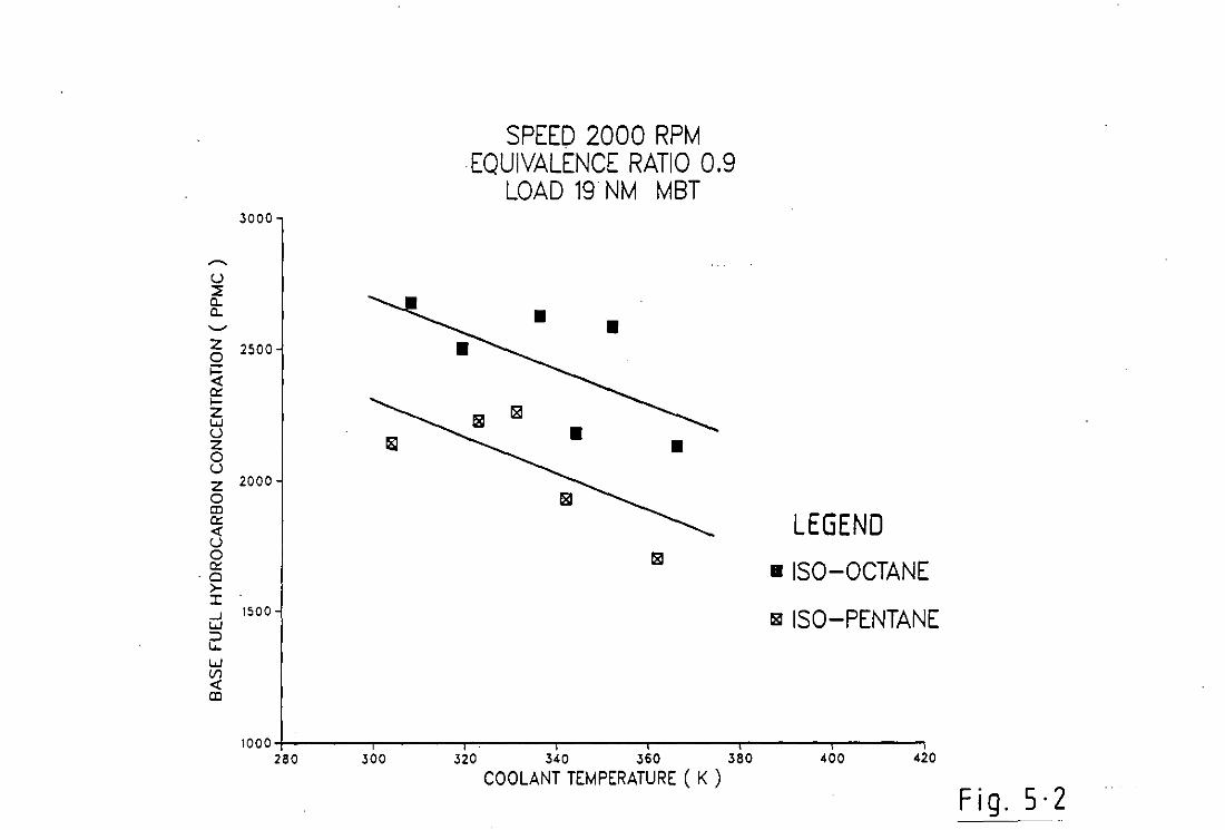
SPEED 2000 RPM EQUIVALENCE RATIO 0.9
LOAD 19 NM MBT 3000
,-...
U ~ a.. a.. '-"
Z 2500 0
< a:: ;-Z w U Z 0 U Z 2000 0 CD
LEGEND a:: <! U 0 a:: • ISO-OCTANE -0 >-::r: ...J 1500
~ ISO-PENTANE w ::> u.. w tIl <! CD
1000 2BO 300 320 340 360 3BO 400 420
COOLANT TEMPERATURE ( K ) Fig. 5·2

SPEED 1000 RPM ~QUIVALENCE RATIO 0.9 LEGEND
LOAD 14.3 NM MBT 4000 • ISO-OCTANE
,...... Ilil ISO-PENTANE u • ~
Q - ISO-OCTANE -=- 3500 ---- -Z • • 2000 RPM 0
~ - - - • • Cl::: - - -~ - -Z - -w 3000 - -U -Z -0 -U Z 0 Cl) Cl::: « 2500 U 0 ~ a ~ J: ...J W :::> 2000 L.o..
W III « Cl)
1500 300 310 320 330 340 350 360 370
COOLANT TEMPERATURE ( K )
Fig. 5·3

~
'...)
1-"'" ---'
Z 0 ~ <: c: '-z w U Z 0 u z 0 ~ c: <: u 0 c: 0 >-I
,000
. 2500·
2000
1500
SPEED 2000 RPM EQUIVALENCE RATIO 0.9
LOAD 19 NM MBT
•
~~
•
•
LEGEND
• ISO OCTANE
~ ISO-PENTANE
1000 +---~-~--.,-.---.~ ........... -,----_-_-..--..--,................-,...., 1 10 100
1/HENRY CONSTANT ( IN SQUALANE )
Fig. 5·4

4000
~ 3500
U :::; C. C.
---Z 3000 0 >= < 0:: >-Z u U 2500 z Q u z 0 ::l 0:: 2000 < u 0 0:: Cl ;.-
!500
SPEED 1000 RPM . EQUiVALENCE RATIO 0.9
LOAD 14 .. 3 NM MBT
10 1/HENRY CONSTANT ( IN SQUAlANE )
LEGEND • ISO OCTANE
181 ISO-PENTANE
100
Fig. 5·5

CHAPTER 6
REFERENCES AND APPENDICES

REFERENCES
(1) J.A. Lorusso, E.W. Kaiser and G.A. Lavoie
In-Cylinder Measurements of Wall Layer Hydrocarbons in a Spark
Ignited Engi ne.
Combustion Science and Technology, 1983,Vol.33, pp.75-112
(2) A.A.Adamczyk, E.W.Kaiser, J.A.Cavolowsky and G.A.Lavoie
An Experimental Study of Hydrocarbon Emissions From Closed Vessel
Expl os ions
Eighteenth Symposium (International) on Combustion
The Combustion Institute, 1981
(3) C.K.Westbrook, A.A.Adamczyk and G.A.Lavoie
"A Numerical Study of Laminar Wall Quenching"
Combustion Institute, October 1979
Combustion and Flame, in Press.
(4) W.A. Daniel and J.T. Wentworth(1962)
Exhaust Hydrocarbons - Genesis and Exodus
SAE Paper No. 486B
(5) J.T. Wentworth(1968)
Piston and Ring Variables Affect Exhaust Hydrocarbon Emissions
SAE Paper No. 6B0109
(6) J.T. Wentworth
The Piston Crevice Volume Effect On Exhaust Hydrocarbon Emission
Combustion Science and Technology, 1971, VolA, pp.97 - 100
(7) Wayne A. Daniel (1970)
Why Engine Variables Affect Exhaust Hydrocarbon Emission
65

SAE Paper No. 700108
(8) P. Weiss and J.C. Keck(1981)
Fast Sampling Valve Measurements of Hydrocarbons in the Cylinder of a
CFR Engi ne.
SAE Paper No. 810149
(9) A.A.Adamczyk, E.W.Kaiser and G.A.Lavoie
Single-Pulse Sampling Valve Measurements of Wall Layer Hydrocarbons
in a Combu st i on Bomb
The Combustion Institute, 1981
(10) J.C. Dent and P.A. Lakshminarayanan(1983)
A Model for Absorption and Desorption of Fuel Vapour by Cylinder
Lubricating Oil Films and it's Contribution to Hydrocarbon Emissions.
SAE Paper No. 830652
(11) W.A. Daniel (1967)
Engine Variable Effects on Exhaust Hydrocarbon Composition (A Single
- Cylinder Engine Study with Propane as the Fuel)
SAE Paper No. 670124
(12) Marvin W. Jackson(1966)
Effects of Some Engine Variables and Control Systems on Composition
and Reactivity of Exhaust Hydrocarbons
SAE Paper No. 660404
(13) G.A.Lavoie, J.A.Lorusso, A.A.Adamczyk
Hydrocarbon Emissions Modelling For Spark Ignition Engines
Published in "Combustion Modeling in Reciprocating Engines"
Symposium 1978, Michigan Proceedings
Edited by J.N.Mattavi and C.A.Amann
Publ ishers Plenum 1980
(14) J.T. Wentworth(1971)
Effect of Combustion Chamber Surface Temperature on Exhaust
66

Hydrocarbon Concentration
SAE Paper No. 710587
(15) M. Namazian and J.B. Heywood(19B3) Flow in the Piston-Cy1inder-Ring Crevices of a Spark-Ignition Engine : Effect on Hydrocarbon Emissions, Efficiency and Power SAE Paper No. B20088
(16) K.T. Dishart and W.C. Harris
The Effect of Gasoline Hydrocarbon Composition on Automotive Exhaust Emi ss ions Proc. Div. Refining,
American Petroleum Institute (1968), Vol. 48, pp. 612 - 642
(17) R. D. F1eming The Effect of Fuel Composition on Exhaust Emissions from a Spark Ignition Engine. Bureau of Mines Automotive Exhaust Emissions Program. Technical progress report 48 RI No. 7423 Sept.'70
(18) J.T.Wentworth(1972) More on Origins of Exhaust Hydrocarbons - Effects of Zero Oil Consumption, Deposit Location, and Surface Roughness. SAE Transactions 720939
(19) M.W. Jackson, W.M. Weise and J.T. Wentworth(1962) The Influence of Air-Fuel Ratio, Spark Timing, and Combustion Chamber Deposits on Exhaust Hydrocarbon Emissions SAE Paper No. 486A
(20) W.W. Haske11 and C.E. Legate(1972) Exhaust Hydrocarbon Emissions from Gasoline Engines - Surface Phenomena
SAE Paper No. 720255
67

(21) G.A.Lavoie and P.N.Blumberg
A Fundamental Model for Predicting Fuel Consumption, NOx and
Hydrocarbon Emissions of the Conventional Spark-Ignited engine
Combustion Science and Technology, 1980,Vol.21,pp.225-258
(22) Keiichiro Shin, Yukio Tateishi and Shoichi Furuhama(1983)
Measurement of Oil-Film-Thickness Between Piston Ring and Cylinder.
SAE Paper No. 830068
(23) E.W. Kaiser, J.A. Lorusso, G.A. Lavoie, A.A. Adamczyk (1981)
The Effect of Oil Layers on the Hydrocarbon Emissions from Spark
Ignited Engines.
Combustion Science and Technology,1982,Vol.28, pp. 69 - 73
(24) A.A. Adamczyk and R.A. Kach (1983)
The Effect of Oil Layers on Hydrocarbon Emissions: Low Solubil ity
Oils
Combust ion Sci ence and Technology, 1981, Vol.25, pp. 9-19
(25) C.C. Chappelow, III and J.M. Prausnitz
Solubilities of Gases in High-Boiling Hydrocarbon Solvents.
A.I. Ch.E. Journal 20 P.1097 (1974)
(26) G.Carrier,F.Fendell, P.Feldman
Cyclic Absorption/Desorption of Gas in a Liquid Wall Film
Combustion Science and Technology,1981, Vol.25 pp. 9 - 19
(27) LW.Kaiser, A.A.Adamczyk and G.A.Lavoie
The Effect of Oil Layers on the Hydrocarbon Emissions Generated
During Closed Vessel Combustion
Eighteenth Symposium (International) on Combustion
The Combustion Institute, 1981
(28) A.A.Adamczyk and R.A.Kach
A-Combustion Bomb Study of Fuel-Oil Solubility and Hydrocarbon
Emissions from Oil Layers
68

Twentieth Symposium (International) on Combustion, 1984, pp.37-43
(29) R.S. Spi ndt(1965)
Air-Fuel Ratios from Exhaust Gas Analysis.
SAE Transactions 650507
(30) F.G. Rounds, P.A. Bennett and G.J. Nebel
Some Effects of Engine-Fuel Variables on Exhaust-Gas Hydrocarbon
Content
SAE Transactions, Vol. 63 (Jan), 1955, pp. 591-601
(31) J.N. Shi nn and D.R. 01son(1957)
Some Factors Affecting Unburned Hydrocarbons in Engine Combustion
Products
SAE Paper No. 146
(32) A.J.P. Martin
Symposium on Gas Chromatography. Analyst 81, 52 (1956)
(33) Saing, H.G.Harris, and J.M.Prausnitz
Henry's Constants for Methane, Ethane, Ethyl ene, Propane, and
Propylene in Octadecane, Eicosane, and Docosane
(Jou rna 1 of Chemi cal and Engi neeri ng Data)
Vol.14, No.4, October 1969
69
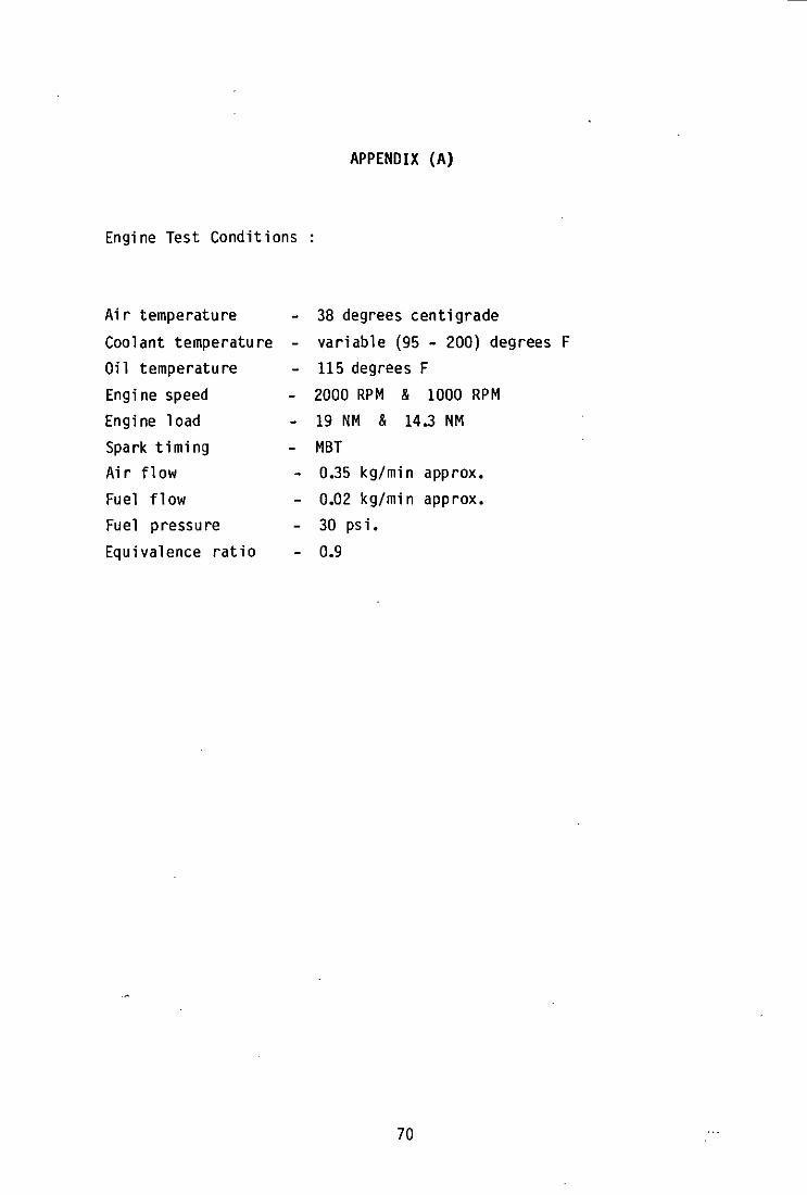
APPENDIX (A)
Engine Test Conditions
Air temperature - 38 degrees centigrade
Coolant temperature - variable (95 - 200) degrees F Oil temperatu re
Engine speed Engi ne load
Spark timing Air flow
Fuel flow Fuel pressure
Equivalence ratio
- 115 degrees F
- 2000 RPM & 1000 RPM
- 19 NM & 14.3 NM
M8T
- 0.35 kg/min approx. - 0.02 kg/mi n app rox. - 30 ps i.
- 0.9
70
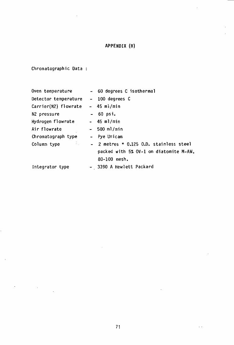
Chromatographic Data
Oven temperature
Detector temperatu re
Carrier(N2) flowrate
N2 p ressu re
Hydrogen flowrate
Air flowrate
Chromatograph type
Column type
Integrator type
APPENDIX (B)
- 60 degrees C isothermal
100 degrees C
- 45 ml/min
- 60 psi.
- 45 ml/min
- 500 ml/min
- Pye Unicam
- 2 metres * 0.125 O.D. stainless steel
packed with 5% OV-1 on diatomite M-AW.
80-100 mesh.
3390 A Hewlett Packard
71

APPENDIX (Cl
Engine and General Specification
Type
Number of cyl i nders
Bore
Stroke
Swept vo 1 u me
Maxi mum speed
Maximum power
Comp ress i on rat i 0
Va 1 ve arrangement
Fuell i ng
Ignit ion system
Cooling
Lubrication oil
Special Fuels
Gasoline Ricardo Hydra
1
80.26 mm
88.9 mm
450 ml
90 rev/sec
15 kw
11 : 1
twin overhead camshaft, vertical valves
petrol injection, 12 volt Bosch
pump feeding twin injectors,
injector type: Bosch 0280 150 151
Lucas SP 12 coil with lumenition
spark plug : champion N6Y
Ignition timing: photo-electric cells
with printed circuit board counter.
Adjustment - manual.
- closed circuit system with heat
exchanger.
82.5 % Mi d-east base oil
15.5 % Additive packing
2 % Viscosity improver
Viscosity grade 20/40
Iso-pentane : Research Analar Grade
minimum assay 99 %
contai ns 1 % n
pentane.
Iso-octane Shell Research Grade
72

APPENDIX (D)
Typical PPM C Levels (2000 RPM at 19 NM load)
Fuel Iso-octane
Methane & Ethane - 180 to 420 PPM C
Propane 180 to 240 PPM C
n-Butane
Is o-penta ne
n-Hexane
n-Heptane
Iso-octane
Fuel Iso-pentane
- 360 to 540 PPM C
- Approx. 5 PPM C
- Negligible
Negligible
- 2400 to 3500 PPM C
Meth ane & Eth ane - 420 to 570 PP M C
Propane
n-Butane
Iso-pentane
n-Hexane
n-Heptane
Iso-octane
- 240 to 270 PPM C
- 100 to 140 PPM C
2400 to 3200 PPM C
- Negl i gi b 1 e
Negligible
- Approx. 40 PPM C
73

PROGRAM LISTINGS
APPENOIX E - CALCULATION OF AIR/FUEL RATIO
APPENDIX F - DATA REDUCTION PROGRAM
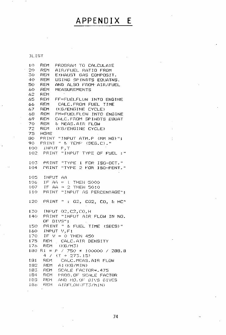
APPENDIX E
] L T ~~T
1 (I REI"! PF:OG!::;:I~i'1 Tt] CPILCULATE 20 REM AIR/FUEL RATIO FROM 30 REM EXHAUST GAS COMPOSIT. 40 REM USING SPINDTS EQUATNS. 50 REM AND ALSO FROM· AIR/FUEL 60 REM MEASUREMENTS 62 RE~I
66 67 68 69 70 72
RE~l
F:EM REM RE!"I REM RE~l
REt1 75 HOI"IE
FF=FUELFLOW INTO ENGINE C{lLC- FHO~I FUEL TTME
(KG/ENGINE CYCLE) FM=FUE!.FLDW INTO ENGINE C?,LC. Fi.;DI1 SPII'lOTS EQUAT ~<: MEAS. t-~ I F~ FLOl.&J (KG/ENGINE CYCLE)
BO PRI!~T" INPUT ATi1. P (/'11'1 HG)"; 90 Pr": J ~H ,; ~" TEI"IF" (DEG. C) • " 100 iNPUT F:rT 102 Pf.: I NT 11 I I\~F'UT T'lF'E OF FUEL :"
1 03 PF, I NT "TYPE 1 FOF: I SO-OCT. " 104 PF:INT "TYPE 2 FOH ISO-PENT."
1 05 I j'-!PUT ;~A
106 11= AA = i THEN '5000 107 IF AA = 2 -rHEN 5010 110 F'r~II\JT "INF'UT (:t£; PEF=:CEr,jTAGE";
170 PRINT I. : 02, C02, CO, Bc He'l
1.40 PF:INT" INPUT PoIR FLOvJ IN NO. OF DIV~3";
150 F'~:INT" ~< FUEL. TIME (SECS)" 160 INPUT '..', F 1 170 IF V = 0 THEN 450 175 REI~ CALC.AIR DENSITY 176 REM (KG/M3) 180 RI =.P / 750 * 100000 / 288.8
1<31 182 183 18.(~
4 / REI"1 F<:EI1 I':EI1 !":EM PEI'I ";1:-:1"1
er + 27:'::;~ 15)
CALt2.MEAS.AIR FLOW ,0.1 (!<:G/MJ.N) SCAl_E !=ACTOR=.475 PROD.OF SCALE FACTOR Af~D !,!O.O~ llIVS GIVES ?ilj=::FI.. .. UvJ (r=T~:./l'"iIN)
74

lCj~:' nE!'! (!<G/r-·ll!'.!;' .1. \i~j !. F :=4:·:; ::; ::: THE},! .20.2 196 REM FUEL BURETTE - 82CC 1Q7 R!~M REl_.I)ENS.OCTANE - .7()3 198 Hi = .C)8~ .~ .703 * 60 ! Ft 200 i::.JCJ~·D:;~.1.~)
201 F:EI-l I':I::L. DEI~S. FENT ANE - • 6::::6
202 HI = .082 * .626 * 60 / Fl 203 REM CALC.FUEL MASSIKGiCYCLE
i 205 FF ::; Ml / 1000
!:ALC. ME~S.A!F RATIO ~210 Z :~; (ij / f"'11 220 F·r:: I i·,JT If 11
23!) PRIN·r "MEASURED AIR FLOW -
24() F'r:;:T!\lT (~l;" (Vi3/1'1It-J) ,.
245 Al = Al / J.OOO
" " ~;
260 F'j::;Il\jT !'1·' ~ I, 1«3/f'"lI~.j"
265 ~Jl = H1 I 1000 270 PRINT "AIR/FUEL RATIO = ";Z .27~2 F'F~INT "{;l!·-:;; FLtJl~J ~<G/CYCLE = "
~2"/4 F'r:;~Ji\jT ';FUEL. j"1f~~3~:; (I<G/C:VCL~E) F
27~i
276 280 2 ci'O r' :~::;oo D .,. 1 Ct r~~
:320 C
F:iJri 1':E}"l
F:Et"1 I F
..
,-
,.,
FUEL TINE::; ":: Ml CALC. A/F RATIO FROM SPINDTS' EQUATIONS
02 60 GO TO 440 CO j C~~
Cl:::: :" C2 (CO + C2) / (CO + C2 -!- J-I)
(C2 ~- co .~ H) I <8.63 + .
578 ~ C2 - .422 * 02 + .784 * CD ·1 1." 206 .1>: '·0
325 REM CALL. A/F RATIO 330 A = F * (1.1.492 * C * «(1 + R
-" ··.'·7
12+ Q) / (1 + R» + 1.20 .~
(:I _ ... C) / (3.5 + F;:»)
REM CALC.FUEL FLOW FROM I':E:L'I :=;P I NOT!,>' EQUAT . {l iF .·,;[::IV ! r:;(';T I 0 ,~ .. j'·1EAS. {; I FFt._O~'J
75

::::;35 FM = Ai / ;.) :AO PF:INT 350 PF:Ii'JT "EXH'4L1ST COMPOSITION' :
" 360 PRINT "OXY = " nr , .. " ( :~ ) ...:....!"
= " CS''' " C~) , ~. !" 370 PF:INT "C02
= " CO; " ( i: ) , 380 PI~INT "CO "
= " H; " (i: ) , 390 PRINT "HC "
400 PRINT "A/F RATIO = ";A 405 PRINT "FLlELf"LOvJ FROM SPINDTS
" . , 406 PRINT" = I';FM;" KG/CYCLE" 410 PRINT "C = ";C 420 PRINT "(I-C)/C =";(l-C)
/ C 430 432
REM REI·!
434 REM 436 REI1 440 A =
ROUTINE TO CALCULATE AVERAGE MOLECULAR IoJT. OF FLASK SAMPLE BY 110LAR BALANCES
450 H I (6 ... CO)
8 = C2 / CO 460 C = 02 / CO 470 D = 1 + B + 6 ... A 480 REM DEFINE MOLAR EQTS. 490 Al = (U * A) / D 500 A2 = (U * B) / D 510 A3 = U / 0 520 A4 530 A5 540 A6
= = =
(U ... (W + (y +
/ D Al +
86 ...
C' I D l.>-J
.,. B J "* El
A2 + A3
Al + 44
+ X ... ?) )
+ G ... A
+ A4 +
... A2 +
/ + U
A5
28
D ...
+
...
Cl 550 E =
A6 560 F =
A3 + A6
... A4 + 18 ... A5 + 28 *"
570 M = FIE 575 GC = 8 .. 314 / M 580 PRINT "AV.MOL.WT.EXHAUST =
; t1 582 PRINT 583 PF: I NT 585 PRINT 590 GOTO 600 STOP 4900 REI1 ,4905 F:Et1 4910 REI1 4915 RE!·I 4920 F:EM 5000 U - c· co
1111
"GAS CClNST. = ";GC .. It
110
SUBPROGRAM SPECIFYING VARIOUS CClNSTANTS FOR OCTANE AND PENTANE USED IN THE MOLECULAR l·JE I GHT CALCIJLAT I IJN.
76

::j(lI)i l·J _. S' ::,002 X = 2 5003 Y = 8_ .::, -_. 5004 .J = I 'O- S 5005 G = - 1 5006 GOTO 1 10 5010 1I -- S 5011 t·) = 6 5012 X -- I 5013 Y = = = J_J
5014 J = 8 5015 G = 0.5 5016 GOTO 110
77

APPENDIX F
]LIST
10 HOME 15 PRINT "DATA REDUCTION PROGF:AM
20 REI"! DATA REDUCTION PROGRAM 30 REM CALCULATES HYDROCARBON 32 REM COMPONENT CONC.IN FLASK 33 REM SAMPLE USING SAMPLE AREA
34 REM RATIOS & RESPONSE FACT. 35 REM ALSO CALCULATES 36 REM HYDROCARBON COMPONENT 37 REM F:ESPONSE FACTOF:S FROM 38 REM KNOW~ MASS CONC. 39 REM AND AREA RATIOS 50 REM CONSTS. 60 REM MOL.WTS. 62 REr1 NOS. IN BF:ACKETS F:EFEF: 63 REN TO NO.OF CARBONS IN 64 REM HYDROCAF:E<ON COMPONENT 65 REM lIE. (1) - METHANE) 70 f1t,...J ( 1) = 16 80 Ml·J (2) =30 '7'0 r'll~ (3) = 44 100 NeJ (4) = 58 1 1 (> MeJ ( 5) = 72 120 MvJ (6) = 86 130 Ml'J(7) = 100 140 MW(8) = 114 150 REM GAS CONSTS. 160 R(1) = 0.5196 170 R(2) = 0.2771 180 R(3) = 0.189 190 R(4~ = 0.1433 200 R(~) = 0.1155 210 R(6) = 0.0967 220 R(7) = 0.0831 230 R(8) = 0.0729 260 PF~INT" 11
270 PRINT "INPUT NO.COMPONENTS";
280 INPUT Y 290 PRINT "" 300 PF:INT "DO YOU l'JISH TO RECALI
81~:ATE .......
3(12 PRINT '·(lE.·ft] OBTAIN NEW RES F'Ot·ISE F?\CTOf~:S)"
::;03 PR I NT "YES=2, NO= 1 " :::;10 PF:INT 3:-:::0 I r·JPUT Z 330 IF Z = 1 THEN 890 335 REM INPUT CALIB. DETAILS 340 PF: I NT "I NF'UT FL.A~)!< TE!'"iF"S _ "
78

350 PRINT !Ill
360 FOR N = 1 TO Y 365 IF N = 7 THEN 400 370 PRINT 1111
380 PRINT "T";N; 11=,.; 390 INPUT T(N) 400 NEXT N 410 PRINT "" 420 PRINT "INPUT PAF:TIAL PRESSUF:
ES" 430 FOR N = 1 TO Y 435 IF N = 7 THEN 470 440 PRINT "" 450 PRINT lip"; N; n==:"; 460 INPUT P U·j) 470 NEXT N 480 PRINT "" 510 HOME 520 F:EI'l CALCS 530 FOR N = 1 TO Y 535 IF N = 7 THEN 550 550 NEXT N 560 FOR N = 1 TO Y 565 IF N = 7 THEN 580 570 M(N) = O.726E - 3 * PIN)" I (R
(N) *' (T(N) + 273») 580 NEXT N 590 PF: nn "" 600 FOR N = 1 TO Y 605 IF N = 7 THEN 62b 610 PRINT "P"; N; "=11; P (N) 620 NEXT N 630 PRINT "" 640 FOR N = 1 TO Y 645 IF N = 7 THEN 660 650 PRINT "MII;t-J; "==:";t-1CN) 660 NEXT N 670 PRINT "" 680 REM CONTINUE STATEMENT 690 INPUT "TO CONTINUE TYPE l";Z
79

~·~oo HOME 710 REM INPUT CALIB.AREA RATIOS
7--::"·\ PF:INT .... 73(, PRINT "INPUT CALIB.AF:EA RATI
OS" 740 PRINT 750 FOR N = 1 TO Y 755 IF N = 7 THEN 780 760 PRINT "CALIB.AREA RATIO ";N; .. - .. ~ - , 770 INF'UT CR (N) 780 NEXT N 790 FOR N = 1 TO Y 795 IF N = 7 THEN 810 800 RFINI = CRINI * MI61 I MINI 810 NEXT N 820 PF\INT 11"
830 PRINT "RESPONSE FACTOF:S AF:E: "
840 FOR N = 1 TO Y 845 IF N = 7 THEN 860 850 PF:INT "RF "; N;" = "; RF 1Nl 860 NEXT N 861 PF:II~T "" 870 GOTO 950 880 REM ENTER RESPONSE FACTORS 890 1.1582 895 .9 900 .9023 910 .8626 920 1.18 930 1 935 RF(SI = 1.1704 940 PRINT "," 945 INPUT "TEST NO. = ";TN 950 PF:INT "ENTER TYPE OF FUEL US
EDu 960 PRII~T" 1 FOR OCTANE" 970 PF:INT "2 FOR . PENTANE" 980 INPUT Z 990 IF Z = 1 THEN 1020 1000 A$ = "ISO PENTANE" 1010 GO TO 1040 1020 A$ = "ISO-OCTANE" 1030 REM CALC. SAMPLE ~< I. S.I·JT 1040 HOME 1045 INPUT 11 {-lTMOS. PRESS. 0111HG)=
"; AF' 1050 ·II'iPLlT "ENTf=:R SAt1PLC:: GAS CDN
ST .. ,,; f.:S
1060 1l'IPUT "ENTER SANPLE P/PRESS t-1!1HG "; PS
1070 II'WUT "ENTER ~~AMPLE TEI1P DE
1080 I NF'UT .. ENTEF: IS I·JT. IN I<G .. ; IS
80
1035 INPUT "AIR MASSIKG/CYCLE)= "; AM
1090 PRINT "FUEL MASSIKG/CYCLE)"
1 092 PR I NT .. FRO~l ?\FR CALC. = "; 1095 INPUT FM 1100 REM CALC. SAMPLE MOL.!.oJT. 1110 MS = S.314 I RS 1120 REM CALC. SAMPLE WT. 1130 SW = 110.726E - 3) * PS) / I
RS .. 1ST + 273» 1140 REM CALC. r.S.(~T.
1160 PRINT .... 1170 PRINT "ENTER SAMPLE AREA RA
TIOS:" I1S0 FOR N = 1 TO Y 1185 IF N = 7 THEN 1205 1190 PRINT "SAMPLE . AREA RATIO ... ,
N" " = ... , , 1200 INPUT SRIN) 1205 NEXT N 1207 FOR N = 1 TO Y 1208 IF N = 7 THEN 1230 1210 CIN) = ISHIN) .. IS) / IHFIN)
.. S!.oJ) 1220 PMIN) = CIN) .. MS * N .. liE +
6) / 16 .. M!.oJ(N» 1230 NEXT N 1232 IF Z = 1 THEN L = 8 1233 IF Z = 2 THEN L = 5 1234 FL = CIL) .. SW 1235 PT = PMll) + PM(2) + PM(3) +
PM(4) + PM(5) + PMIS) 1236 Fa = FL .. lAM + FM) / SW 1237 D = Fa .. lOO/FM 1238 TL =7.814E - 8 ~ AP .. FL 1240 F:EM PR I NT OUT MASS FRACT I
ON 1250 HOME 1260 PHINT A$,"TEST ";TN 1280 FOR N = 1 TO Y 1285 IF N = 7 THEN 1300 1290 PRINT "MASS FRAC. ";N;"= ";
81
\
C (1'0 1300 NEXT N 1320 FOR N = 1 TO Y 1325 IF N = 7 THEN 1340 1330 PRINT "PPM(HEX) COMP. ";N;"
= ";PM(N) 1340 NEXT N 1342 PRINT "TOTAL PPM HEX = ";PT
1343 PRINT "TOTAL PPM C = "; (6 * PT)
1345 PRINT "SAMPLE WT.= ";SW;" K G "
1350 PRINT "FLASK FUEL MASS = "; FL; "KG!!
1360 PRINT "FUEL OUT = ";FO;" KG /CYCLE"
1370 PRINT "TEST LOOP FUEL MASS = ";TL;II KG"
1380 PRINT "FUEL OUT AS % OF FUE L IN= ";D
82
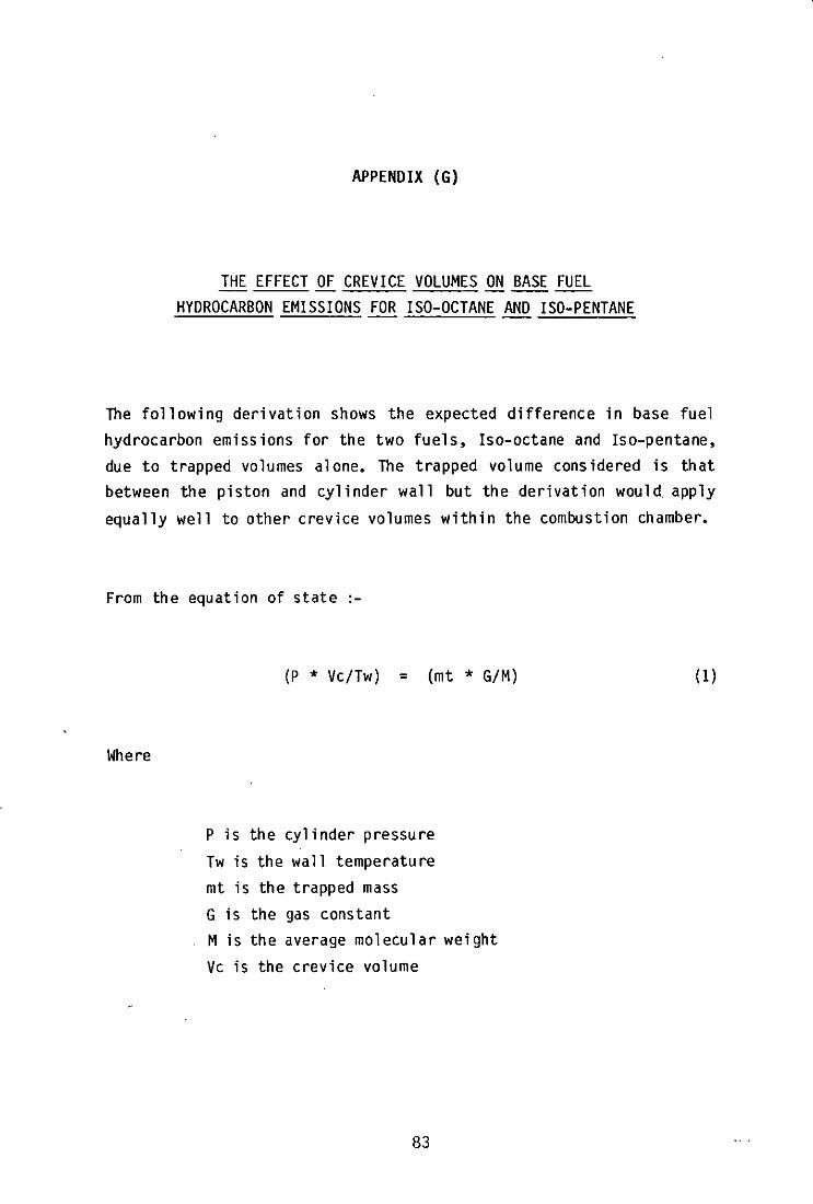
APPENDIX (6)
THE EFFECT OF CREVICE VOLUMES ON BASE FUEL HYDROCARBON EMISSIONS FOR ISO-OCTANE AND ISO-PENTANE
The following derivation shows the expected difference in base fuel
hydrocarbon emissions for the two fuels, Iso-octane and Iso-pentane,
due to trapped volumes alone. The trapped volume considered is that
between the piston and cylinder wall but the derivation would. apply
equally well to other crevice volumes within the combustion chamber.
From the equation of state
Where
(P * VC/Tw) = (mt * G/M)
P is the cylinder pressure
Tw is the wall temperature
mt is the trapped mass
G is the gas constant
M is the average molecular weight
Vc is the crevice volume
83
(1)

Cl ea rly
Where
mt = (ma + mf) = mf(ma/mf + 1)
M = ma * Ma + mf * Mf -------ma + mf
= (ma/mf) ~ Ma ~ Mf
(ma/mf + 1)
ma is the trapped ai r mass
mf is the trapped fuel mass
Ma is the molecular mass of air
Mf is the molecular mass of the fuel
(2)
(3 )
The crevice volume, Vc, will be the same for both fuels. For a given
wall temperature with other engine conditions remaining constant for
both the fuels, it follows that the cylinder pressures for both cases
will also be about the same.
It follows from (1)
(mt *G/M)o = (mt * G/M)p (4 )
84

Where the suffixes
o denote Iso-octane
p denote Iso-pentane
By appropriate substitution of equations (2) and (3) into (4) the
expression becomes :
mfp ~ [(ma/mfp)+1]2 = mfo ~ [(ma/mfp)+1]2
[(ma/mfp)*Ma + Mfp] [(ma/mfo)*Ma + Mfo]
Therefore the trapped fuel mass ratio for Iso-octane and Iso-pentane
is given by :
mfo
mfp
= [(ma/mfp )+1]2
[(ma/mfo)+1]2
* [(ma/mfo)*Ma+Mfo]
[(ma/mfp)*Ma+Mfp]
Stoichiometric air/fuel ratios for
Iso-octane = 15.05
Iso-pentane = 15.25
(5 )
Since all tests were carried out at an equivalence ratio of
approximately O.g for both fuels then:
A/F rat i 0 of Is o-octa ne = 16.72
A/F rat i 0 of I so-pentane = 16.94
85

Molecular mass of
Air = 29
Iso-pentane = 72 Iso-octane = 114
Substitution of these figures into equation(5) gives :-
mfo = 1~9 * mfp ~)
At given conditions where the engine is run at fixed speed, load, water temperature and equivalence ratio for Iso-octane and Iso
pentane :-
(1) Iso-octane emissions should be about 9 percent greater than those of Iso-pentane due to crevice volumes alone.
(2) Any absorption/desorption effect should show up on top of this 9 percent.
In order to give a more conservative estimate to the absorption/desorption effect this figure of 9 percent has been rounded up to 10 percent. The extra 1 percent would help to allow for any other small hydrocarbon sources which may also contribute unequal levels of hydrocarbons for the two fuels.
86
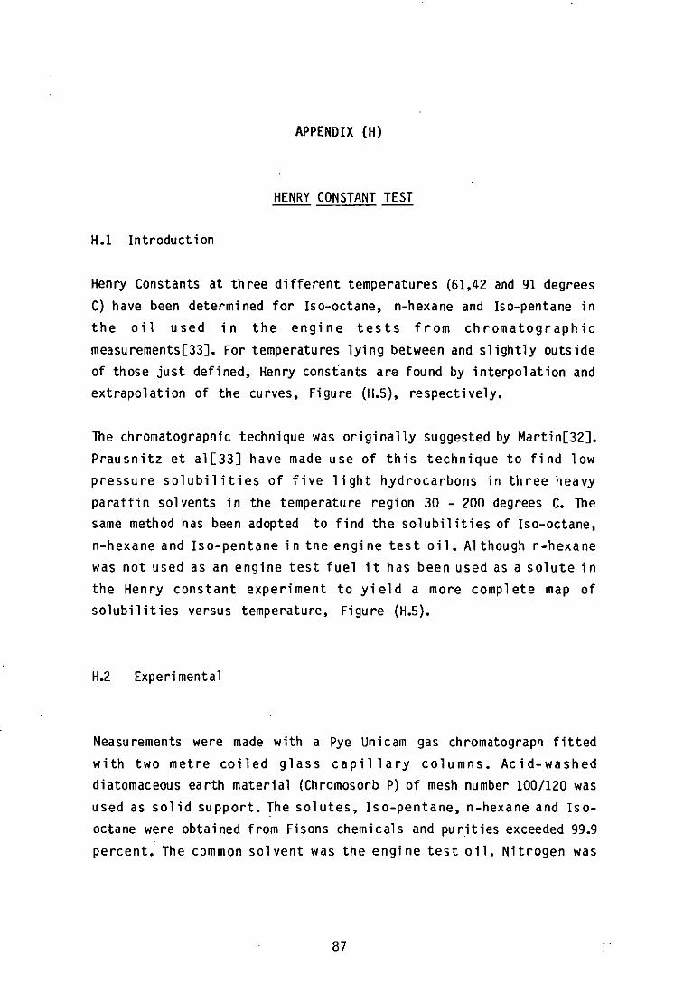
APPENDIX (H)
HENRY CONSTANT TEST
H.l Introduction
Henry Constants at th ree different temperatures (61,42 and 91 degrees
C) have been determined for Iso-octane, n-hexane and Iso-pentane in
the oil used in the engine tests from chromatographic
measurements[33]. For temperatures lying between and slightly outside
of those just defined, Henry constants are found by interpolation and
extrapolation of the curves, Figure (H.5), respectively.
The chromatographic technique was originally suggested by Martin[32].
Prausnitz et a1[33] have made use of this technique to find low
pressure solubi1ities of five light hydrocarbons in three heavy
paraffin solvents in the temperature region 30 - 200 degrees C. The
same method has been adopted to find the solubilities of Iso-octane,
n-hexane and Iso-pentane in the engi ne test oil. Although n-hexane
was not used as an engine test fuel it has been used as a solute in
the Henry constant experiment to yi e1d a more comp1 ete map of
solubilities versus temperature, Figure (H.5).
H.2 Experi menta 1
Measurements were made with a Pye Unicam gas chromatograph fitted
with two metre coiled glass capillary columns. Acid-washed
diatomaceous earth material (Chromosorb P) of mesh number 100/120 was
used as sol id support. The sol utes, Iso-pentane, n-hexane and Iso
octane were obtained from Fisons chemicals and purities exceeded 99.9
percent. The common sol vent was the engi ne test 0 i 1. Nitrogen was
87
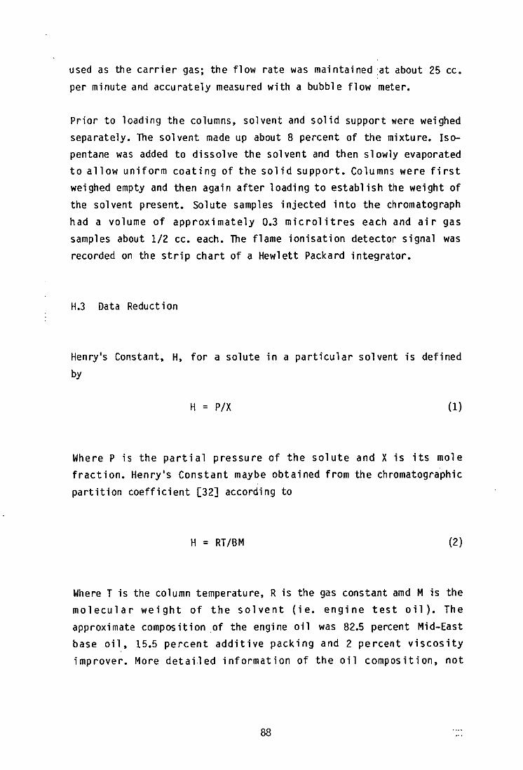
used as the carrier gas; the flow rate was maintained ,at about 25 cc.
per minute and accurately measured with a bubble flow meter.
Prior to loading the columns, solvent and solid support were weighed
sepa rate ly. The sol vent made up about 8 percent of the mi xtu re. Is 0-
pentane was added to dissolve the solvent and then slowly evaporated
to allow uniform coating of the solid support. Columns were first
weighed empty and then again after loading to establ ish the weight of
the solvent present. Solute samples injected into the chromatograph
had a volume of approximately 0.3 microlitres each and air gas
samples about 1/2 cc. each. The flame ionisation detector signal was
recorded on the strip chart of a Hewlett Packard integrator.
H.3 Data Reduct ion
Henry's Constant, H, for a solute in a particular solvent is defined
by
H = P/X (1)
Where P is the partial pressure of the solute and X is its mole
fraction. Henry's Constant maybe obtained from the chromatographic
partition coefficient [32J according to
H = RT/BM (2)
Where T is the column temperature, R is the gas constant amd M is the
molecular weight of the solvent (ie. engine test oil). The
approximate composition .of the engine oil was 82.5 percent Mid-East
base oil, 15.5 percent additive packing and 2 percent viscosity
improver. More detailed information of the oil composition, not
88

available, was required to assess the molecular weight of the oil.
The molecular weight of the engine oil was assumed to be the same as
that for squalane (ie. 422). The plots shown in Figures(5.4) & (5.5)
are in terms of the reciprocal of Henry constant which is linearly
dependent on the molecular weight of the oil (see equation (2)). The
actual value for molecular weight is unimportant since it is only the
trends that are of interest in Figures(5.4) & (5.5).
The partition coefficient, B, is defined as the ratio of the mass of
solute per gram of solvent to the mass of solute per cc. of gas at
column temperature. For a given system, B, is related to peak
retention time, tr, by
B = (tr - tm) j VI W (3)
Where tm is the peak retention time of an essentially insoluble gas
(air), sec.; V is the flow rate of carrier gas at column outlet
pressure and temperature, cc. per sec.; and W is the weight of
solvent in the column, grams.
The pressure correction factor, j, is given by
j = 1.5(P2i n/p20ut - 1)
(P3i n/p 30ut - 1)
(4 )
Where Pin is the pressure at the inlet of the column and Pout is the
pressure at the outlet of the column.
A schematic of the apparatus is shown in Figure(H.1) and tabulated
data is found in Table(H.1). Chromatograms for the three fuels (Iso
pentane; n-Hexane and Iso-octane) at the three temperatures (61,42
and 91 degrees C) are given in Figures(H.2),(H.3) & (H.4). The
89
average peak retention time was found from three chromatograms for each fuel/temperature setting but for simplicity only one chromatogram per fuel/temperature combination is shown in the
Figures.
90
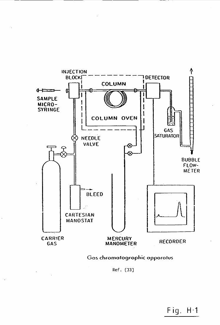
INJECTION
G-I. le " ,
SAMPLE MICROSYRINGE
CARR!ER GAS
BLOCKI - - - - - - - - -, DETECTOR I COLUMN I ,----, I I I I
L-J ~-.J
I I I I I I I COLUMN OVEN I L ______ _
NEEDLE VALVE
-BLEED
CARTESIAN MANOSTAT
I
GAS SATURATOR
BUBBLE FLOWMETER
MERCURY MANOMETER RECORDER
Gas chromatogrophic opparatus
Ref. [33]
Fig. H·1

CHROMATOGRAMS (WITH ELUTION TIMES)
• COLUMN TEMPERATURE 42 C
2-01 MI N. ISO-PENTANE
-----------' 5·85 MI N.
n- HEXANE
_----------' 13·62 MI N.
ISO-OCTANE
Fig. H·2
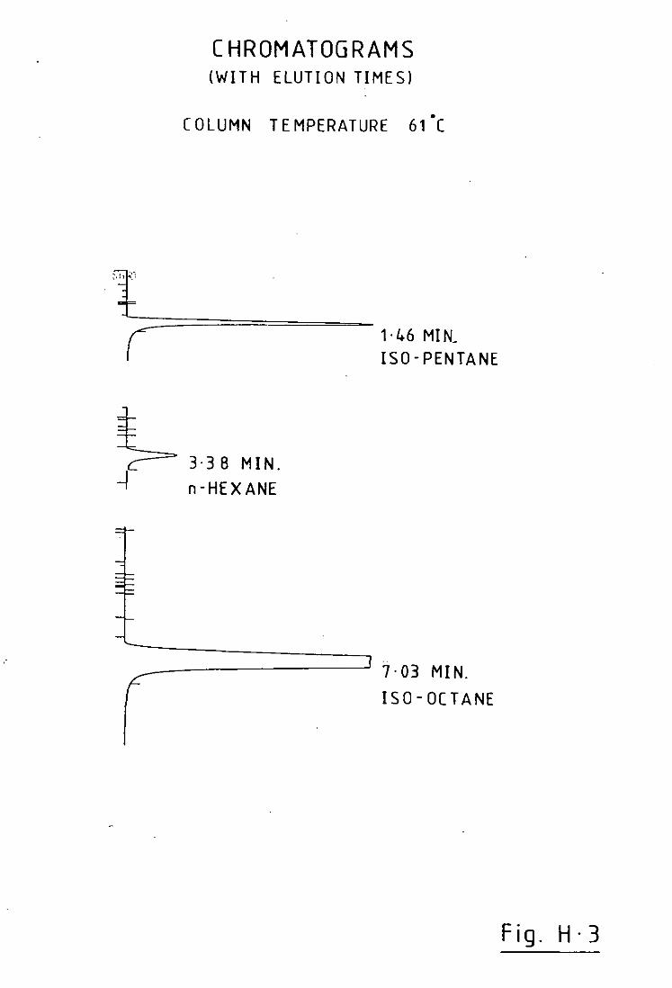
1':'
[ HROMATOGRAMS (WITH ELUTION TIMES)
• COLUMN TEMPERATURE 61 C
'+ '--(=========~ 1·46 MIN_
ISO - PENTANE
3·38 MIN.
n-HEXANE
----------' 7·03 MI N.
ISO-OCTANE
Fig. H·3

,
I
I I
(HROMATOGRAM S (WITH ELUTION TIMES)
o
COLUMN TEMPERATURE 91 C
.~========~ 1·04 M IN.
,1·79 MIN. n-HEXANE
----=====- .3·14 MIN.
ISO-OCTANE
ISO-PENTANE
Fig. H·4

...J
·0 fVl W f-W Z (3 Z w Z
1
- 0.1 -....;
fZ ~ Vl Z o U
>a:: z w I
USING MOL. WT. OF SQUALANE FOR ENGINE OIL
LEGEND • ISO-PENTANE
o ISO-OCTANE
~ N-HEXANE
o.ot+---,---,.--,----,-----,---,.--,----,----,------, 300 310 320 330 340 350 360 370 380 390 400
COOLANT TEMP[RATURE ( K )
Fig. H·5

'<7" I
lJ.J .....J CO <! I-
0 Z
E-< UJ [i) E-<
1
2
3
U 0 -"' 0:: ::>
~ [i)
'" lE [i) E-<
Z lE ::> ..< 0 U
T 61 61 61 91 91 91 42 42 42
U l.? 0
'" -~ "' - 0::
~ "' 0:: ::> UJ '" UJ
~ [i) 0::
'" E-<
u u H H 0:: 0:: [i) [i)
'" '" '" '" UJ UJ 0 0
~ lE
~ <t:
PA TA 753 16 753 16 753 16 753.5 15.5 ·753.5 15.5 753.5 15.5 753 16 753 16 753 16
G l.? .~ ~ ..:
0 -- - E-<
'" z ::> 0:: H 0 ::>
~ [i) '" 0:: 0:: ::> ::>
'" UJ UJ
'" UJ UJ
~ '" gj 0:: E-< '" '" ~ ~ ~ ::> ::> ::> ..< ..< ..< 0 0 0 U U U
T PIN POUT 334 1631 757.5 334 1631 757.5 334 1631 757.5 364 1737.5 757 364 1737.5 757 364 1737.5 757 315 1577 757 315 1577 757 315 1577 757
_ .. -
0:: 0:: ~~ 0 0 ::>u r.- r.- ..< u
'" 0-
"' [>j ~ u ~ -~
H UJ E-< E-< '" ",Z
~ iE ~ Z 0
H H ~ ~ ~ ~[;l S~ ..< ~U ~~ r.-
~~ ~
[i) [i) gj", gj~ 0:: UJ - ~~ HlE
~e1 ~~ ~g cl '" <t: "'UJ u- uo
tM tR V 43.2 . 421.4 25 .4787 43.2 202.8 25 .4787 43.2 87.2 25 .4787 41.8 188.4 25 .5233 41.8 107.4 25 .5233 41.8 62.4 25 .5233 43.8 817.8 25 .4518 43.8 349.8 25 .4518 43.8 119.6 25 .4518
-
E-< Z z "' 0 H
H U E-< H u r.-[i) r.-gj '" 0 0 U u [i) ~ 0:: H ::>0:: E-<
gj~ H
~ "'U 0:: <t: '" r.- '"
j B .6072 250.7 .6072 105.8 .6072 29.17 .5772 100.98 .5772 45.19 .5772 14.19 .623 496.8 .623 196.4 .623 48.7
E-<
1l! E-< UJ
~ U
>< 0::
ffi '" H
.0583
.1381
.5008
.1576
.3523 1.1218
.0277
.0702
.2833
..< [i) ::> r.--[i) E-< ::> ..< 0 UJ
iso-octane n-hexane iso-pentane iso-octane n-hexane iso-pentane iso-octane n-hexane iso-pentane
e:( fe:( Cl
fVl w f-
fz: e:( fVl Z Cl U
>-0:: Z W :I:

-x -Cl Z L.L.J 0... 0... <l:
u • -~
~ "-
~ u ~
0:
'" ::: '" ~
18.5 17 17 17.5 16.5 17.5 19.5 19.5 20 19.5 20 14 13.5 16 16.5 17.5 17.3 18 16 17.2 18.5 17.7 15.5
i -~ :>
~ .U
H .1!l :: "-
~ 765.8 761.6 747.5 746.8 753 754 751 751. 3 753.2 753.2 751.7 751.5 751. 7 762.1 750 745.6 751.6 764 762.6 763.4 732 749.2 752.7
u • ;;; - • [;1 -~
.,
~ ~ ~. ~
~ H
0: H .:
38 115 38 145 38 175 38 95 37.5 160 38 200 38 68 38 193 38 155 38 122 38 137 39 135 38.5 155 38.5 190 38 86 38 135 38 152 38 90 38 185 38 110 38 105 38 145 38 190
.. • -i N
~ 8 Z .. ::: ! • -
~ -- to " ~ Z
~ ~ H
..l 15 H '" £;j 0 III E-
115 2000 18.3 24 12.2 115 2000 18.8 24 12.1 115 2000 18.3 24 12.1 115 2000 17.9 24 12.2 115 2000 18.2 24 12.15 115 2000 18.4 24 12.2 115 2000 16.8 24 11.8 115 2000 17.7 24 11.8 a5 2000 17.7 24 11.8 115 2000 17 24 11.8 115 2000 17.8 24 11.65 115 1000 14.3 20 11. 7 115 1000 14.3 20 11.5 115 1000 ·14.3· 18 11.6 115 1000 14.3 22 11.6 115 1000 14.3 26 11.8 115 1000 14.3 26 11.8 115 1000 14.3 26 11.9 115 1000 14.3 26 11.7 115 1000 14.3 26 11.85 115 2000 14.3 34 11.9 115 2000 14.3 34 11.75 115 2000 14.3 34 11.85
,
~ .,
~ 0
~ 8 N H 0 .~ -.. .. .. - - - .,
~ ~ ~ '" ~ to ~ 0 ~ z
~ ~ ta ~ tl ., B ~ ~ £;j £;j £;j :;! i;!. H
r. E- ..: f-
.082 2.9 .37 16.77 iSQ-octane 2512 . 8 I ..: Cl
.087 2.85 .37 16.82 " 2627 2 f-
.091 2.95 .36 16.86 " 2580 3 Vl w
.088 2.8 .39 16.7 " 2669 4 f-
.088 2.95 .36 16.83 " 2184 5 LU eT>
.091 2.9 .33 16.81 " 2132 6 z: -.091 3.13 .32 17.22 iso-pentane 2158 7
.09 3.1 .258 17.35 • 1702 8 '-" z: w
.088 3.1 .27 17.29 • 1934 . 9
.091 3.1 .3 17.24 • 2236 10
.09 3.05 .3 17.36 • 2274 11
.083 2.6 .33 17.13 • 2570 9 12
.095 2.75 .325 . 17.34 " 2311 13
.08 2.55 .24 17.34 • 1944 14
.09 2.8 .35 17.34 • 2824 15
.082 2.5 .41 16.91 iso-octane 3248 16
.085 2.6 .38 16.98 • 3404 17
.072 2.5 .42 16.82 • 3436 18
.06 2.45 .4 16.99 · 3250 19
.08 2;55 .415 16.88 • 3697 20
.08 2.75 .45 16.85 • 3203 21
.081 2.55 .42 16.95 • 3148 22
.089 2.65 .39 16.94 " 2882 23 --

APPENDIX (J)
THE SOLUBILITIES
OF ISO-OCTANE AND ISO-PENTANE ~ SQUALANE
The following discussion indicates the reasons behind using Iso
octane and Iso-pentane as fuels in an engine test to demonstrate the
significance of the absorption/desorption effect. Figure(J.l) shows
data from Reference [25] displayed as lines of constant temperature.
in the variation of Henry's Constant for a range of paraffins
dissolved in Squalane. It should be noted that the greater the Henry
constant for a given paraffin/oil combination the lower the
solubility is of the paraffin in the oil. Since modelling[26],[lO]
and experiment[23],[24],[27] have indicated the fuel/oil solubility
dependence of the absorpt ion/desorption mechanism the work in th is
thesis has aimed to use this characteristic to show the relative
significance of this mechanism on exhaust hydrocarbons.
The requirement was to run an engine on two fuels whose solubilities
in oil differed appreciably and thereby determine the magnitude of
the absorption/desorption effect from differences in exhaust
hydrocarbons measured for the two fuels. Since the choice of fuels
was subjected to other constaints such as availability, octane number
and more importantly a criterion to keep the fuel system of the
engine unchanged, two 1 iquid fuels were finally chosen, Iso-octane
a nd I so-pentane.
It is evident from Figure(J.l) that the Henry Constant for Iso
pentane is at least a factor of ten greater than that for Iso-octane
dependin.g on temperature. Therefore providing that hydrocarbon
contribution from other sources, su~h as crevices and deposits,
remain approximately the same for both fuels any difference in
92

exhaust hydrocarbons between Iso-octane and Iso-pentane for a gi ven
set of engine conditions could be attributed to the
absorption/desorption effect. However it was found that th is
assumption was not entirely correct and details of this are given in
Appendix(G) •
93

10J
z :: lQ ,-z o v
-'" >-
~ l.'
Il
0·:1
47SK
~ : 42SK
~
:z ~ '2 Z ... z' :r ... ~ ... X· ~
~ - ~ :> >: ~. a> . , I.
20 40 60 SO \ f\-!l \ ~ 1:0 140 160 ,..OlECUl AR '011
-l2SK
VARIATION OF HENR{S (ONSTANT fOR RANGE OF PARAFFINS OISSOL VEO IN SOUALANE ((lO Hn I.
DATA FROM REF. [25]
Fig_ J-1
