an experimental performance evaluation of spatio-temporal

An Experimental Performance Evaluation of Spatio-Temporal Join

Strategies

Seung-Hyun Jeong, Norman W. Paton, Alvaro A. A. Fernandes, Tony GriffithsDepartment of Computer Science, University of Manchester,

Manchester M13 9PL, UKemail: (jeongs,norm,alvaro,griffitt)@cs.man.ac.uk

May 8, 2004

Abstract

Many applications capture, or make use of, spatial data that changes over time. This requirementfor effective and efficient spatio-temporal data management has given rise to a range of research activ-ities relating to spatio-temporal data management. Such work has sought to understand, for example,the requirements of different categories of application, and the modelling facilities that are most effec-tive for these applications. However, at present, there are few systems with fully integrated supportfor spatio-temporal data, and thus developers must often construct custom solutions for their applica-tions. Developers of both bespoke solutions and of generic spatio-temporal platforms will often need tosupport the inter-relating of large spatio-temporal data sets. Supporting such requests in a databasesetting involves the use of join operations with both spatial and temporal conditions – spatio-temporaljoins. However, there has been little work to date on spatio-temporal join algorithms or their evaluation.This paper presents an evaluation of several approaches to the implementation of spatio-temporal joinsthat build upon widely available indexing techniques. The evaluation explores how several algorithmsperform for databases with different spatial and temporal characteristics, with a view to helping de-velopers of generic infrastructures or custom solutions in the selection and development of appropriatespatio-temporal join strategies.

1 Introduction

Real world objects are naturally associated with space and time: spatial information represents positionsand/or extents of the objects in space, and temporal information represents the existence of the objects intime. When the spatial properties of an object evolve over time, the object has a history of spatial data.

A significant number of applications in fields such as the Earth Sciences, Cartography and Land Infor-mation Systems involve the storage and analysis of large amounts of historical spatial data (e.g. [4, 5, 26]).Such data can be challenging to represent and manage, giving rise to much work on, for example, ST(Spatio-Temporal) data models [31, 3, 8, 6] and indexing techniques [17, 29, 19]. We note, however, thatthe development of systems that provide comprehensive support for spatio-temporal data is challenging,and that many application developers have resorted to custom solutions in the absence of widely avail-able generic solutions. For example, a survey of experience managing spatio-temporal data describingadministrative boundaries is given by [5], in which many custom-built systems are described.

Many applications that associate collections of spatio-temporal data on the basis of their aspatialand temporal properties are likely to end up developing or using spatio-temporal join algorithms. In STdatabases, ST join queries, that combine two sets of ST objects according to join predicates embracingboth spatial and temporal attributes, are likely to be important and expensive. For example, a spatio-temporal join query can identify which bus routes passed through a town in 2001. Surprisingly, however,there has been much less attention given to ST join algorithms in the literature than to, for example,spatio-temporal data models or indexes. In this context, this paper contributes to the understanding of STjoins by introducing and evaluating strategies for processing ST join queries. It is hoped that these resultswill be of interest not only to the developers of spatio-temporal data management systems, but also to thedevelopers of custom applications.

1

Although there has been little work on ST joins, some adjacent areas have been extensively explored.For example, there has been intensive research on spatial join algorithms (e.g., [2, 16, 21]) and temporaljoin algorithms (e.g., [25, 32]) employing diverse index structures, hash tables, and sort-merge techniques.In this paper, the strategies are implemented using techniques based on index structures, following Index-based Nested-Loop [7, 18] and Synchronized Tree Traversal [2, 32] approaches, as discussed further in Section2. As such, the paper shows how approaches proposed for supporting spatial joins can be extended foruse with spatio-temporal data, and describes a performance evaluation of the resulting implementations.This activity can be seen to complement research on other aspects of spatio-temporal querying, which, forexample, has investigated algorithms for moving objects [15] or for identifying nearest neighbours in spaceand time [24].

As the ST join algorithms employed in this paper might be considered to be “obvious” extensions oftheir spatial counterparts, the principal contribution is the experimental evaluation of the approaches ratherthan the algorithms themselves. The experiments compare alternative strategies over various databasesizes, numbers of snapshots and input selectivities, using ST data collections generated by GSTD [28], aST data generator. Although there have been several performance studies of spatial and of temporal joinalgorithms before, we know of no comparable study for spatio-temporal joins. In the absence of such astudy, developers lack hard evidence on which to base design decisions that may be important to theirdevelopment activities. Synthetic data is used because of the control it provides in support of experimentdesign, in which it is often necessary to vary a single factor at a time in order to understand the effect thatfactor has on performance. Clearly the risk exists in studying algorithms in use with synthetic data thatthis data is not representative of that found in real applications. However, although some benchmarks usereal data (e.g. [27]), this approach may also involve unrepresentative data, and current practice in spatialdata management seems to favour synthetic data for performance studies (e.g., [30]).

This paper is structured as follows : Section 2 presents an overview of existing spatial and temporal joinalgorithms; Section 3 describes the processing of ST joins; Section 4 explains the design of the experimentsincluding QEPs (Query Execution Plans); in Section 5, an analysis of the experimental results is given;and lastly in Section 6, some conclusions are drawn from the experiments.

2 Related Work

Join algorithms are typically classified as hash-based, sort-merge-based, or index-based, depending on thedata structure or data property exploited by the algorithm. Spatial and temporal join algorithms can alsobe classified into these groups. This paper, however, focuses on index-based algorithms, as (i) indexes onspatial, temporal and ST attributes of objects are likely to be widely available, as many different queryoperations can benefit from their presence; and (ii) previous evaluations of spatial (e.g., [1]) and temporal(e.g., [32]) joins testify to the effectiveness of index-based approaches.

Well known index-based spatial and temporal join algorithms fall into two groups: Index-based Nested-Loop (INL) [7, 18] and Synchronized Tree Traversal (STT ) [2, 32]. INL is a variant of the simple nested-loopalgorithm, where each object of the outer collection is scanned, and the join attribute of the object is usedas the search key to an index structure for the inner collection. The pseudo-code for an INL algorithmis given in Figure 1 using an intersection predicate. In the INL algorithm, each index lookup for theinner collection is independent of all other lookups to that collection. Thus the index is accessed in anuncoordinated manner.

The main idea of STT is to reduce the number of visits to internal nodes of two index trees by traversingthe indexes of the operands synchronously, as illustrated in Figure 2 for spatial joins with intersectionpredicates.

INL is specifically useful when only one operand is indexed (as may be the case, for example, for joinsinvolving intermediate results), while STT requires indexes on both operands. Note that the intersectionpredicates in line 2 of SpatialLookup() and in line 3 of SpatialSTT () can be replaced with other predicates,e.g. a containment predicate.

Index-based join algorithms are, of course, affected by the index structures used, and various structuresfor spatial and temporal indexes have been proposed. This section focuses on R-trees [9] as R-trees canbe applied to spatial [9], temporal [12] and ST data [29]. R-trees have also been shown to perform well inboth spatial [1] and temporal [32] join algorithms, and are widely available (e.g. in the PostgreSQL DBMS(www.postgresql.org)). This paper can be seen as providing insights into the use of widely available indexes

2

SpatialINLJoin(R, rootTS , O)input:

R, a collection of spatial objects;rootTS , the root node of TS , the R-tree indexing the join attribute of S, the other input collection;

output:The result O is a collection of pairs of objects from R and object identifiers from S;

/* es is an entry in leaf nodes of TS which is a pair of MBR, mbr, and an object identifier, oid;r is an object of R, having val as its spatial attribute;Mbr() is a function that computes an MBR enclosing its argument;S′ is a lookup result which is a collection of es. */

begin1: O := ∅;2: for each object r ∈ R do3: S′ := ∅;4: SpatialLookup(rootTS , Mbr(r.val), S′);5: for each es ∈ S′ do6: O := O ∪ {(r, es.oid)};end.

SpatialLookup(NT , window, O)input:

NT , which is a node of an R-tree; window is a searching area;output:

The result O is a collection of entries in leaf nodes;

/* readNode() returns the R-tree node referred to by its argument. */

begin1: for each e ∈ NT do2: if NT is a leaf node where (e.mbr intersects window) 6= ∅3: then O := O ∪ {(e.oid)};4: else if NT is an internal node where (e.mbr intersects window) 6= ∅5: then SpatialLookup(readNode(e), window, O);end.

Figure 1: An INL Algorithm

such as R-trees, including their 3D extensions [29], for supporting spatio-temporal requests.Note that the algorithms in Figures 1 and 2 correspond to the filtering step [2], in which approximations

(such as Minimum Bounding Rectangles) of the join attribute values are used to reduce the cost of pairwisecomparisons of spatial values; the subsequent refinement step [2] compares the actual values. In whatfollows, all spatial and ST joins require a refinement step, whereas purely temporal joins do not – intervalscan be represented precisely within R-trees.

3 Approaches to Spatio-Temporal Join Processing

In a query language, there is often no specialised syntax for an ST join – it is simply a join with spatialand temporal conditions, as in:

select *from R, Swhere Cs and Ct

In the above query, R and S are input data collections for a join, and Cs and Ct are spatial and temporalconditions respectively.

3

SpatialSTTJoin(rootTR , rootTS , O)input:

rootTR and rootTS , each of which is the root node of R-trees, TR and TS ,over input collection R and S, respectively;

output:O, a set of pairs of object identifiers;

begin1: O := ∅;2: SpatialSTT (rootTR , rootTS , O);end.

SpatialSTT (Nr, Ns, O)input:

Nr and Ns, each of which is a node of an R-tree;output:

O, a set of pairs of object identifiers;

/* an entry of an R-tree node, er and es, is a pair of MBR, mbr, and an object identifier, oid;readNode() returns the R-tree node referred to by its argument. */

begin1: for each er ∈ Nr do2: for each es ∈ Ns do3: if Nr and Ns are leaf nodes where (er.mbr intersects es.mbr) 6= ∅4: then O := O ∪ {(er.oid, es.oid)};5: else if Nr and Ns are internal nodes where (er.mbr intersects es.mbr) 6= ∅6: then SpatialSTT (readNode(er), readNode(es), O);end.

Figure 2: A STT Algorithm

This paper compares three alternative ST join strategies depicted in Figure 3 in relational algebra: (a)performs a spatial join followed by a temporal selection; (b) performs a temporal join followed by a spatialselection; and (c) performs a specialised ST join. In all cases a spatial selection is required to support therefinement step. The conditions representing the filtering and refinement steps are denoted by Cs

′ and Cs

respectively. The prime is also used in Figures 4 and 5 to label the filtering conditions.These alternatives are explored so that experiments can compare specialised ST algorithms with com-

binations of spatial and temporal algorithms for answering ST queries. These comparisons not only assessthe efficiency of the different approaches, but can also inform the decision as to how many indexes arerequired. For example, an ST index enables indexed access to both spatial and temporal data, but may beexpected to be less effective in these cases than the more specialised spatial-only or temporal-only indexes.

The experiments reported in Sections 4 and 5 compare each of the strategies depicted in Figure 3, usingboth INL and STT algorithms for spatial, temporal and spatio-temporal joins.

To implement the strategies, R-trees are used for spatial, temporal and ST joins. The ST joins use 3DR-trees [29], a 3D variant of R-trees in which two dimensions are occupied by space, and time is treatedas a third dimension.

In spatial, temporal and ST joins, the approximate values used in the 2D and 3D R-trees are: normalMBRs (Minimum Bounding Rectangles) represented by two pairs of the x- and y-coordinates of the lower-left and the upper-right corner points of a rectangle (i.e. (xll, yll), (xur, yur)) for spatial indexes; MBRswith upper bound x-coordinates set to the maximum value for the now time point and y-coordinates set tozero for temporal indexes; and MBCs (Minimum Bounding Cuboids) with x- and y-coordinates representingthe spatial dimension and z-coordinates representing the temporal dimension for spatio-temporal indexes.

The STT algorithms used in the implementation adopt the local optimization and search space restric-tion techniques of Brinkhoff et al.’s algorithm [2]. By way of local optimization, the plane sweep [20]technique is used to reduce the CPU time required for comparison of indexed entries from nodes of two

4

R S

./(Cs′)

σ(Ct)

σ(Cs)

(a)

R S

./ (Ct)

σ(Cs)

(b)

R S

./(Cs′∧Ct)

σ(Cs)

(c)

Figure 3: Logical Expressions for ST Joins

distinct R-trees. For the spatio-temporal case, the notion of space sweep [11] is used, which is analogous tothe plane sweep, but for 3D. The first attempt to employ the space sweep for sort-merge-based spatial joinsover 3-dimensional spatial data is found in [21]. The search space restriction technique reduces the numberof indexed entries to be compared at each tree traversal stage by restricting the space of comparison usingthe intersecting area of the two upper level node entries from distinct trees: only the entries overlappingthe intersecting area can be candidates of comparison at the tree traversal stage since only that area is ofinterest for comparison.

4 Experiments

This paper tests the following hypotheses:

(i) Specialized ST joins perform better than spatial joins followed by a temporal selection and temporaljoins followed by a spatial selection.

(ii) Joins using STT algorithms perform better than INL algorithms in ST databases.

(iii) Spatial and temporal joins perform better using spatial and temporal indexes respectively than withST indexes.

These hypotheses would normally be expected to be true, so the interesting cases are those in whichthe hypotheses do not hold. However, as well as testing these hypotheses, the experiments provide manydetails from a range of scenarios that should be useful to the developers of spatio-temporal systems.

4.1 Queries and Query Execution Plans (QEPs)

The tables Cities, BusRoutes and Shops are used as the context for the queries used in the experiments:

Cities(id: integer, description: string, boundary: Polygon, vt: Interval)BusRoutes(id: integer, description: string, centreline: Polyline, vt: Interval)Shops(id:integer, description: string, location: Point, vt: Interval)

A city can change in boundaries by growth or shrinkage and keep a boundary during a time interval; abus route can change to reflect requirements of local areas, for financial reasons, etc; and a shop can oftenchange location for expansion or contraction.

The vt attribute represents the valid time of a tuple in the table. The precise spatial model used is notcrucial to the experiments, as these focus on the filtering step of join processing involving spatial values,using MBRs or MBCs as abstract representations of the centreline, boundary and location attributes. Thusthe results presented in this paper are of relevance in the presence of different spatial models, as long asthese can be abstracted for representation in indexes using MBRs or MBCs.

The following queries are used in the experiments:

5

Q1.1 Which bus routes intersected a city at some time?

select *from Cities c, BusRoutes bwhere c.boundary intersects b.centrelineand c.vt intersects b.vt;

Q1.2 Which shops were contained by a city at some time?

select *from Cities c, Shops swhere c.boundary contains s.locationand c.vt intersects s.vt;

Q2 Which bus routes intersected a city within a given area (represented by a spatial-literal) during agiven period (represented by valid-time-literal).

select *from Cities c, BusRoutes bwhere c.boundary intersects b.centrelineand c.boundary intersects <spatial-literal>and b.centreline intersects <spatial-literal>and c.vt intersects b.vtand c.vt intersects <valid-time-literal>and b.vt intersects <valid-time-literal>;

Q3.1 Which bus routes have at some time intersected an area that at some time was a city?

select *from Cities c, BusRoutes bwhere c.boundary intersects b.centreline

Q3.2 Which shops have at some time been contained by an area that at some time was a city?

select *from Cities c, Shops swhere c.boundary contains s.location

Q4 Which bus routes and cities co-existed at some time?

select *from Cities c, BusRoutes bwhere c.vt intersects b.vt

Queries Q1.1, Q1.2 and Q2 are all spatio-temporal joins, in that their join conditions have both spatialand temporal aspects; the principal distinguishing feature of Q2 from Q1.1 and Q1.2 is that it allows changesto the selectivity of the inputs to the join operations using spatial and temporal selection conditions. Theseconditions are used to vary the selectivity of the inputs to the join, as described in Section 5.4. QueriesQ3.1 and Q3.2 are purely spatial queries run over spatio-temporal data collections – there is no temporalcondition in the join. Similarly, Q4 is a purely temporal query – there is no spatial condition in the join.

Queries Q1.1 and Q3.1 use intersection relationships between spatial values with extent in their ap-proximate representation (viz. polygon and polyline values) for join predicates, but queries Q1.2 and Q3.2involve containment relationships between spatial values with extent and without extent (viz. point values).

To evaluate such queries, a query processor translates a query written in a declarative surface language,e.g. SQL, into a logical query expression as shown in Figure 3 comprising logical operators at internalnodes and input collections at leaf nodes; and that expression is in turn translated into a physical query

6

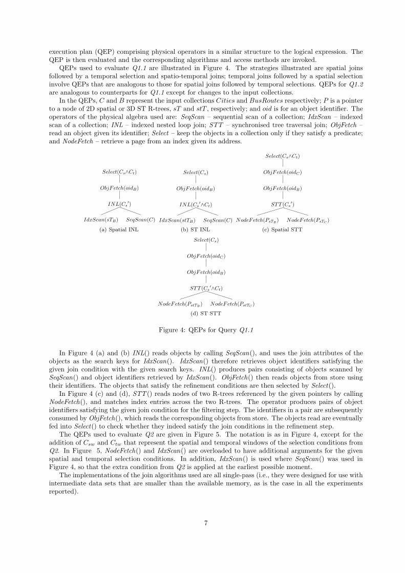
execution plan (QEP) comprising physical operators in a similar structure to the logical expression. TheQEP is then evaluated and the corresponding algorithms and access methods are invoked.

QEPs used to evaluate Q1.1 are illustrated in Figure 4. The strategies illustrated are spatial joinsfollowed by a temporal selection and spatio-temporal joins; temporal joins followed by a spatial selectioninvolve QEPs that are analogous to those for spatial joins followed by temporal selections. QEPs for Q1.2are analogous to counterparts for Q1.1 except for changes to the input collections.

In the QEPs, C and B represent the input collections Cities and BusRoutes respectively; P is a pointerto a node of 2D spatial or 3D ST R-trees, sT and stT , respectively; and oid is for an object identifier. Theoperators of the physical algebra used are: SeqScan – sequential scan of a collection; IdxScan – indexedscan of a collection; INL – indexed nested loop join; STT – synchronised tree traversal join; ObjFetch –read an object given its identifier; Select – keep the objects in a collection only if they satisfy a predicate;and NodeFetch – retrieve a page from an index given its address.

IdxScan(sTB) SeqScan(C)

INL(Cs′)

ObjFetch(oidB)

Select(Cs∧Ct)

(a) Spatial INL

IdxScan(stTB) SeqScan(C)

INL(Cs′∧Ct)

ObjFetch(oidB)

Select(Cs)

(b) ST INL

NodeFetch(PsTB) NodeFetch(PsTC

)

STT (Cs′)

ObjFetch(oidB)

ObjFetch(oidC)

Select(Cs∧Ct)

(c) Spatial STT

NodeFetch(PstTB) NodeFetch(PstTC

)

STT (Cs′∧Ct)

ObjFetch(oidB)

ObjFetch(oidC)

Select(Cs)

(d) ST STT

Figure 4: QEPs for Query Q1.1

In Figure 4 (a) and (b) INL() reads objects by calling SeqScan(), and uses the join attributes of theobjects as the search keys for IdxScan(). IdxScan() therefore retrieves object identifiers satisfying thegiven join condition with the given search keys. INL() produces pairs consisting of objects scanned bySeqScan() and object identifiers retrieved by IdxScan(). ObjFetch() then reads objects from store usingtheir identifiers. The objects that satisfy the refinement conditions are then selected by Select().

In Figure 4 (c) and (d), STT () reads nodes of two R-trees referenced by the given pointers by callingNodeFetch(), and matches index entries across the two R-trees. The operator produces pairs of objectidentifiers satisfying the given join condition for the filtering step. The identifiers in a pair are subsequentlyconsumed by ObjFetch(), which reads the corresponding objects from store. The objects read are eventuallyfed into Select() to check whether they indeed satisfy the join conditions in the refinement step.

The QEPs used to evaluate Q2 are given in Figure 5. The notation is as in Figure 4, except for theaddition of Csw and Ctw that represent the spatial and temporal windows of the selection conditions fromQ2. In Figure 5, NodeFetch() and IdxScan() are overloaded to have additional arguments for the givenspatial and temporal selection conditions. In addition, IdxScan() is used where SeqScan() was used inFigure 4, so that the extra condition from Q2 is applied at the earliest possible moment.

The implementations of the join algorithms used are all single-pass (i.e., they were designed for use withintermediate data sets that are smaller than the available memory, as is the case in all the experimentsreported).

7

IdxScan(sTB , Csw′) IdxScan(sTC , Csw

′)

INL(Cs′)

ObjFetch(oidB)

ObjFetch(oidC)

Select(Cs∧Ct∧Csw∧Ctw)

(a) Spatial INL

IdxScan(stTB , Csw′∧Ctw) IdxScan(stTC , Csw

′∧Ctw))

INL(Cs′∧Ct)

ObjFetch(oidB)

ObjFetch(oidC)

Select(Cs∧Csw)

(b) ST INL

NodeFetch(PsTB, Csw

′) NodeFetch(PsTC, Csw

′)

STT (Cs′)

ObjFetch(oidB)

ObjFetch(oidC)

Select(Cs∧Ct∧Csw∧Ctw)

(c) Spatial STT

NodeFetch(PstTB, Csw

′∧Ctw) NodeFetch(PstTC

, Csw′∧Ctw)

STT (Cs′∧Ct)

ObjFetch(oidR)

ObjFetch(oidB)

Select(Cs∧Csw)

(d) ST STT

Figure 5: QEPs for Query Q2

4.2 System Environment

The experiments have been run using the PostgreSQL 7.1.3 object-relational DBMS. PostgresSQL allowsusers to extend its functionality through user-defined functions and user-defined types. In addition, R-treesare implemented using the GiST (Generalized Search Tree) [10] that is part of PostgreSQL. The GiST isan Abstract Data Type for search trees, which enables users to implement additional index structures. Allthe implementations of physical operators and R-trees rely on the buffer management of PostgreSQL, inwhich 64 8K buffers are used.

The underlying experimental environment consists of a 700MHz Pentium III PC with 256Mb mainmemory running RedHat Linux version 7.2. In the experiments each QEP was run three times, and theaverage used. Each execution is performed after the PostgreSQL server has been shut down and restarted,and the operating system buffer cache has been flushed (i.e., queries are run “cold”).

4.3 Data Generation

For generating data collections of Cities, BusRoutes and Shops a slightly modified version of the datagenerator GSTD [28] has been used. Data collections generated with GSTD can be tuned by variousparameters:

1. The initial cardinality of a collection – this is a straightforward way of varying the sizes of the datacollections being studied.

2. The initial density of a collection (i.e., the percentage100×

∑area of a spatial object

workspace area ) – this can be usedto reflect the fact that different geographical environments may have different numbers of features ina given area.

3. The number of snapshots – this can be used to capture the fact that applications differ in the periodfor which historical data is available and that data capture rates vary.

4. The duration between consecutive snapshots – this can be used to reflect the fact that different datasets may be updated at different rates;

5. The change in location of time-evolving spatial objects – this can be used to capture the nature ofthe changes taking place.

8

Data CollectionsParameters DC1 DC2

number of initial spatial objects 500 to 1500 in steps of 250 200number of snapshots 20 50 to 150 in steps of 25

initial spatial density(%) 0 for point collections; 30 for rectangle collections

change in location(%)[-10%, 10%] of the entire spatial data space at random for point collections;

[-10%, 10%] of extents’ size at random for rectangle collectionsduration between changes(%) [50%, 100%] of time resolution at random

size of objects(bytes) 460distribution uniform

Figure 6: Data Collections

The following parameters are selectively varied to yield databases of different sizes in the performanceevaluation of queries Q1.1, Q1.2, Q3.1, Q3.2 and Q4:

• the initial cardinality of spatial objects; and

• the number of snapshots.

In evaluations involving query Q2, the spatial and temporal windows are varied in size.The data collections used in the experiments simulate only discrete change in the locations of spatial

objects. The change in location of the object with extent in each direction is a random value up to 10% ofthe size of the object in that direction; and when the object does not have extent (i.e. a point) the changeis a random value up to 10% of the entire spatial data space size. Changes happen consecutively after aperiod that is a random value from 50% to 100% of the temporal resolution. The temporal resolution isdetermined by the number of snapshots. The distribution of initial spatial objects, the changes in theirlocation, and the duration between consecutive snapshots follow a uniform distribution.

The details of the data collections used are presented in Figure 6. Thus data collections DC1 and DC2explore changes in database size by varying the number of initial spatial objects and snapshots respectively.Polygon, polyline and point values of Cities, BusRoutes and Shops are approximated by rectangles in thecollections. The data collections are inserted into PostgreSQL tables in chronological order and R-treesare built on the tables. To give an indication of the database sizes used in the experiments, the largestdatabases in both DC1 and DC2 are around 55Mb. We note that the absolute size of the databases is notthe principal issue – the principal issue is the relative performance of the approaches and the growth curvesfor single-pass algorithms; we do not explore cases in which disk space is required to store intermediateresults.

Figure 7 visualises some snapshots of an example data collection, and Figure 8 shows the simplifieddistribution of time intervals of input data collections by transforming 1-dimensional intervals into 2-dimensional points. Intervals of the last snapshots of each spatial object, whose ending instant is themaximum value, now, in the given temporal dimension, constitute the upper distribution.

There is clearly a limit to the number of aspects of a data set that can be changed in an experimentalstudy. This paper has not considered aspects such as data skew, or variable complexities of individualspatial objects. These factors could influence experimental results, and thus could form the basis forcontinuing studies on spatio-temporal join performance.

5 Results

This section presents the results of the experiments, for which the data collections, queries and queryexecution plans were presented in Section 4.

5.1 Varying Spatial Cardinality

This subsection describes how the different join strategies perform using spatio-temporal queries Q1.1 andQ1.2 over data collections in DC1, in which the size of the database is varied as a result of changing thenumber of initial spatial objects. So that the experiment is focused on the number of data items, and notinfluenced by changing density, the initial spatial density of rectangle collections is kept at 30% throughout

9

(a) 200 Rectangles (1st, 75th, 150th snapshots from left)

(b) 200 Points (1st, 75th, 150th snapshots from left)

Figure 7: Examples of Data Collections (with 200 spatial objects)

� � � � � � � � � � � � � � � � � � � � � � � � � � � � � � � � � � � � � � � � � � � � � � � � � � � � � � � � � � � � � � � � � � � � � � � � � � � � � � � � � � � � � � � � � � � � � � ��

� � � � � � � � � � � � � � � �

��

��

��

��

��

� � � � � � � � � � � � � � � � � � � � � � � � � � � � � � � � � � � � � � � � � � � � � � � � � � � � � � � � � � � � � � � � � � � � � � � � � � � � � � � � � � � � � � � � � � � � � � ��

� � � � � � � � � � � � � � � �

��

��

��

��

��

Figure 8: Distribution of Time Intervals

for DC1, which means that 30% of the area is occupied at each point in time. This is done by decreasingthe average area occupied by each spatial object as the cardinality increases.

Figure 9 shows elapsed times for four of the join strategies for Q1.1. To clarify the graphs, the perfor-mance of QEPs using temporal INL and temporal STT joins are excluded from the graphs since they showsignificantly poorer performance than the others. The poor performance of the joins based on temporalindexes arises from the high temporal density of the data collections used. This high density gives rise tosignificant overlaps in interior MBRs of temporal R-trees (and thus inefficient lookup) and to large resultsizes from purely temporal filtering for spatio-temporal joins, which in turn gives rise to high refinementcosts. We note that high temporal densities are realistic overall, as it is to be expected that many dataitems will exist at the same time.

In Figure 9 and hereafter: the spatial, temporal and spatio-temporal INL strategies are referred toas s inl, t inl and st inl, respectively; and the spatial, temporal and spatio-temporal STT strategies arereferred to as s stt, t stt and st stt, respectively.

The results in Figure 9 exhibit several features that are worthy of comment:

(i) The STT algorithms perform better than their INL counterparts. This result can be explained withreference to Figure 10 (a) and (b), where it can be seen that the STT algorithms perform many fewervisits to index nodes than the INL algorithms. This confirms earlier results [2] on the effectivenessof the STT approach over spatial data, and shows that the results, as expected, carry over to joinsover 3D R-trees.

(ii) The st stt (or the st inl) performs better than the s stt (or the s inl). This is principally because thenumber of results returned by the ST join is considerably less than the number of results from the

10

��

� �� !�� "

# $# %& #' ()* +),-

� .�� .� �� .� � � � � .��

Figure 9: Elapsed time for query Q1.1 with data collections DC1

��

�� !�� "�� #

$ %&' ()* +* ,+- ./

0�� !�� 0�� !��

(a)

��

�� !��"��#�� $

% &'( )*+ ,+ -,. /0

� 1�� 1��

(b)

��

�� !��"��#�� $

% &'( )*+ ,+ -,. /0

� � 1� "�� 1� � �

(c)

Figure 10: Number of node visits for the query Q1.1 with data collections DC1

��

� � � �� !� �"��#��$�� %

&' () *+,-./ 01 23

� 4�� #

(a)

��

� �� !"��#��$�� %�� &

'( )* +,-./0 12 34

� 5�� $ � � 5�� $

(b)

Figure 11: Number of join result for the query Q1.1 with data collections DC1

spatial join, as shown in Figure 11. The join selectivity is lower in the ST case simply because thejoin condition is more precise, including both spatial and temporal aspects. The larger join resultfrom the spatial query means that many more objects must be fetched from the store after the join,

11

��

� ��

! "! #$ !% &'( )'*+

,�� ,�� ,� � � � ,� � �


and that many more objects are processed in the refinement step of the join1. We note also that thefigures given here will generally underestimate the cost of the refinement step for real examples, asonly approximations of actual spatial values such as MBRs and MBCs are stored and analysed.

(iii) The st inl performs better than the s stt. In the filtering step of spatio-temporal join processing,the s stt visits many fewer nodes than the st inl as shown in Figure 10 (c). This confirms again theeffectiveness of the coordinated tree traversal technique over the uncoordinated approach as indicatedin (i) above. However, the overall performance does not correspond to the performance of the filteringstep. This can be explained by the fact that there is a significant difference in the number of the joinresults between the st inl and the s stt, which affects the refinement step as indicated in (ii) above,and the cost of the refinement step becomes dominant in the overall join processing.

Figure 12 shows elapsed times for four of the join strategies for Q1.2. The pattern of performance curvesis similar to Figure 9 for Q1.1. It stems from the fact that INL and STT algorithms with containmentpredicates are only different in processing at leaf nodes from those with intersection predicates: viz. in line2 of SpatialLookup() in Figure 1 and in line 3 of SpatialSTT () in Figure 2.

What lessons are learned from this for the developers of ST applications and systems? Perhaps theclearest lesson is that specialised ST indexes were crucial for obtaining scalable performance with ST joins– in the experiment, evaluation strategies that used only spatial or temporal indexes were not competitive.This benefit derived principally from the reduced cost of the refinement step in this case. The performancedifference associated with index selection was more significant than that associated with algorithm selection,although the STT algorithms significantly out-performed INL, as anticipated.

5.2 Varying Number of Snapshots

Figure 13 displays the experimental result of processing the query Q1.1 over data collections DC2. Theseexperiments assess the effect of different numbers of data values from the same geographical area, reflectingdifferent frequencies or periods of data capture. The results in Figure 13 exhibit the following feature thatis worthy of comment:

• As the number of snapshots increases, the benefits from using the ST indexes increase. This isreflected in the fact that st inl and st stt significantly out-perform their spatial counterparts wherethere are large numbers of snapshots. This is to be expected, as the purely-spatial condition testingprovided by the indexes in the s inl and s stt approaches becomes less discriminating as the numberof snapshots increases. This is reflected in Figure 15, where the size of the spatial join result is seento grow more rapidly than that of the ST join.

Figure 16 shows elapsed times for four of the join strategies for Q1.2 over data collections DC2. Thepattern of performance curves is also similar to Figure 13 for Q1.1 as observed between Figures 9 and 12.

What lessons are learned from this for the developers of ST applications and systems? Perhaps theclearest lesson is that specialised ST joins become important as the number of snapshots increases, as

1The large join result from the temporal join illustrated in Figure 11 (a) helps to explain the poor overall performance(not shown but an indication of the poor performance can be derived from Figure 21 for pure temporal joins) of the temporalalgorithms for Q1.1 over DC1.

12

��

� � �� ! "�#�� $

% &% '( %) *+, -+./

0�� 0� � �

(a)

��

� � �� ! "�#�� $

% &% '( %) *+, -+./

� 0�� 0� � �

(b)


��

�� !#"�� $

% &'( )*+ ,+ -,. /0

� 1�� #� � � 1�� #�

(a)

��

� � �� !"�� #

$ %&' ()* +* ,+- ./

0� � � � 0� � �

(b)

Figure 14: Number of node visits for query Q1.1 with data collections DC2

��

� � � � �� !

"# $% &'()*+ ,- ./

� 0�� 1� � � 0�� 1� �

(a)

��

� � �� !"�� #

$% &' ()*+,- ./ 01

� 2� �3� �

(b)

Figure 15: Number of join result for query Q1.1 with data collections DC2

would be expected. This means that developers with historical data collections with shallow histories maywell be able to get by without specialist ST indexing and joins, but that this will become increasingly lessviable as more historical information is accumulated.

Comparing the results in this section and those in Section 5.1, there are differences in the behavioursof the algorithms for the two data collections, with DC1 varying only cardinality (and keeping densityconstant) and DC2 allowing the spatial density to increase as the number of snapshots grows. This givesrise to differences in the numbers of nodes visited for Q1.1 (and Q1.2) with data collections DC1 and DC2,as illustrated in Figures 10 and 14. This can be understood with reference to the spatial, temporal and STdensities in Figure 17. In particular, the spatial density becomes much higher in DC2 than in DC1, whichin turn gives rise to the much larger results for the spatial joins in DC2.

13

��

� � � � ��

! "! #$ !% &'( )'*+

,�� ,� � �

(a)

��

� � �� ! � ��"

# $# %& #' ()* +),-

� � .�� .� � �

(b)


� ��

��

� �� ! �"�#�� #�$�%�& ' ��(�� )� * � ��#�"��+�%��

, -./0 1 23 453 65

� ��

(a) data collections DC1

� ��

��

� � � � � �� ! �" #$� �%� &�� '�!�� ( #$)�* �$+��

, -./0 1 23 453 65

� ��

(b) data collections DC2

Figure 17: Density for DC1 and DC2

5.3 Pure Spatial and Pure Temporal Joins

In the above experiments, ST queries are evaluated using spatial, temporal and ST join strategies. In thissection, joins with purely spatial and purely temporal conditions are run over the same range of strategies.In these examples the refinement step is identical in each case (i.e., the filtering steps all return the samenumber of results for the purely spatial or purely temporal joins, respectively), so all time differences mustbe attributed to the number of node visits in the filtering step and the quality of R-trees in preservingclusters of physical addresses of spatio-temporal data stored, which can affect the costs of object fetchoperations in the refinement step. In the st inl and st stt algorithms only spatial (or temporal) informationis used to to search and traverse the 3D R-trees.

Firstly, the purely spatial join:

Q3.1 over DC1 and DC2 The results in Figure 18 show several features: (i) The STT algorithms out-perform their INL counterparts (i.e., st stt is faster than st inl, and s stt is faster than s inl); and (ii)The specialist spatial joins perform somewhat better than their ST counterparts (i.e. s stt is fasterthan st stt, and s inl is faster than st inl). This latter result is principally explained by the fact thatthe number of node visits of the spatial specialists is usually less than that of STT counterparts asshown in Figure 19.

Q3.2 over DC1 and DC2 The results in Figure 20 show very similar performance for the different al-gorithms to that in Figure 18.

Secondly, the purely temporal join:

Q4 over DC1 As to the pure temporal join algorithms over DC1 the results in Figures 21 (a) confirmsthe efficiency (i) of STT algorithms over their INL counterparts (i.e., st stt is faster than st inl, andt stt is faster than t inl); and (ii) of the specialist temporal joins over their ST counterparts (i.e.t stt is faster than st stt, and t inl is faster than st inl). In pure temporal joins, the benefit usingthe temporal indexes is increasing as the density is much higher in the temporal dimension than in

14

��

� �� !�� "

# $# %& #' ()* +),-

� .�� .� �� .� � � � � .��


��

� � �� ! "�#�� $

% &% '( %) *+, -+./

� 01� �� 0�� 0�� 0��


Figure 18: Elapsed time for the pure spatial query Q3.1

��

�� !��"�� #�� $

% &'( )*+ ,+ -,. /0

� 1�� "�� 1�� "�� 1� � � � � 1� � �


��

� � �� ! �� "

# $%& '() *) +*, -.

� /� !� � � /� !� � /� � � � � /� � �


Figure 19: Number of node visits for pure spatial query Q3.1

��

� �� !

" #" $% "& '() *(+,

-�� -�� -� � � � -� � �


��

� � � � �� !

" #" $% "& '() *(+,

-.� �� -�� -� � � � -� � �


Figure 20: Elapsed time for the pure spatial query Q3.2

the spatial dimension of DC1 as shown in Figure 17. The number of node visits shown in Figure22 (a), however, is not a good guide as to the behaviours of the algorithms. Since the number oftemporal join results is large, as indicated in Figure 11, the cost of object fetch operations becomesthe dominant factor of the overall join processing in this case. Figures 21 (a) and 22 (a) imply thatST indexes can provide better temporal clustering over spatio-temporal data than temporal indexes.

Q4 over DC2 Figures 21 (b) over DC2 shows interesting behaviours of algorithms for pure temporal joinscompared with those over DC1: (i) the efficiency of STT algorithms over their INL counterpartsis still sustained; and (ii) all the specialist temporal joins, however, perform poorer than any STalgorithm. In essence, the principal difference from the same query and algorithms for DC1 is thatthe spatial density of DC2 is considerably higher than that of DC1, but the temporal density is stillconsiderably high compared with the spatial density, as indicated in Figure 17. Figures 21 (b) and22 (b) imply that ST indexes provide not only better temporal clustering than temporal indexes,

15

��

� �� !

" #" $% "& '() *(+,

� -�� -�� -� � � � -� � �


��

� �� !�� "

# $# %& #' ()* +),-

� .�� .�� .�� .��


Figure 21: Elapsed time for the pure temporal query Q4

��

� �� !�� "�� #

$ %&' ()* +* ,+- ./

� 0�� !�� 0� !�� 0�� 0��

(a) data collections DS1

��

� � � � �� !

" #$% &'( )( *)+ ,-

� ./� �� .0� �� .� � � � � .� � �

(b) data collections DS2

Figure 22: Number of node visits for query Q4

but also good physical clustering over the given spatio-temporal data collections. Variations of R-trees used as temporal indexes are found in [12, 13, 14]. [22] provides analysis of such R-tree basedtemporal indexes. Although they show good performance characteristics on average for querying,they sometimes behave pathologically and performance becomes quite poor.

What lessons are learned from this for the developers of ST applications and systems? The experimentsshow that purely spatial joins perform quite well over ST indexes, which suggests that it will not alwaysbe necessary to maintain both spatial and ST indexes in ST applications with both spatial and ST queries.This is an encouraging result, in that reduced storage overheads and update times result from fewer indexes.

We observe, however, that both the temporal and the ST indexes seem to be necessary to obtainadequate temporal join performance depending on data collections.

5.4 Varying Selectivity

Some join strategies are sensitive to the selectivity of their inputs (e.g., this is important when comparingnavigational and value-based joins in object databases [23]). Figure 23 shows the elapsed times for Q2 overone of the databases from DC1 (i.e. 1000 spatial objects × 20 snapshots), for varying input selectivities. Wenote that few radical changes can be seen from the results reported, but that from those shown and othersobtained for lower selectivities (not shown), it seems that the differentials observed for large selectivitiesare somewhat diluted for lower selectivities. This topic could benefit from a more thorough investigation.

6 Conclusion

This paper has described several approaches to the evaluation of spatio-temporal joins and described acomparative evaluation of the approaches. We know of no other similar study.

In terms of the hypotheses described in Section 4, the following can be observed:

16

��

��

��

�� !�" ��#$

� %�� &' � � %� &' � %�� %��

Figure 23: Elapsed time for Q2 for varying selectivities

(i) Specialised ST joins perform better than spatial joins followed by a temporal selection and temporaljoins followed by a spatial selection. This hypothesis is supported by the results in Figures 9, 12, 13and 16. It is clear that in certain cases specialist ST joins provide significantly better performancethan joins using purely spatial or temporal filtering steps, and thus that the extra overhead associatedwith maintaining ST indexes can be beneficial. The benefits from use of specialised ST joins areparticularly great for data sets with large numbers of snapshots, where ST joins substantially reducethe number of candidates forwarded to the refinement step (see, for example, Figure 15). Conversely,where data sets are in use with modest numbers of snapshots, the benefits from using specialised STjoins are much reduced.

(ii) Joins using STT algorithms perform better than INL algorithms in ST databases. The good behaviourof STT joins that is familiar from spatial databases essentially carries over to ST databases. STTperforms much better than INL where there is high density, as shown in figures for elapsed time,and in particular, this is likely to be common in the temporal dimension of ST databases. Thusthere is some evidence that STT approaches will be even more effective in ST databases than theyhave been shown to be in earlier work on spatial databases. However, the experiments show thatthe difference in performance for ST joins is influenced more by the use of specialised ST indexesthan by the specific join algorithm used (see, for example, Figures 12 and 13). For data sets withlarge numbers of snapshots, the use of ST indexes can provide orders of magnitude improvements inperformance, as illustrated in Figure 16.

As STT requires indexes on both operands, and thus is not directly usable over intermediate join re-sults, more work is required to understand the trade-offs involved in building indexes for intermediatecollections.

(iii) Spatial and temporal joins perform better using spatial and temporal indexes respectively than withST indexes. This hypothesis was broadly true in the experiments for spatial joins, but not to theextent that we anticipated. In the spatial experiments (Figures 18 and 20) the performance of boththe STT and the INL approachs over the ST indexes were generally close to the times recorded forthe spatial joins using spatial indexes. This suggests that ST indexes may be able to support querieswith purely spatial conditions.

The hypothesis did not hold for all the cases of temporal joins depending on configurations of inputdata collections: when spatial density is fixed and temporal density increases, there is clear benefitfrom using specialised joins (Figure 21 (a)), but in the reversed case, specialised joins performed lesswell than those using ST indexes (Figure 21 (b)). This was something of a surprise, and may suggesteither that ST indexes can be quite widely employed, or that R-trees are not particularly effectiveas temporal indexes. Further study is required to understand behaviours of R-trees in the mixtureof spatial and temporal dimensions where the two dimensions show different characteristics, e.g. indensity.

In reporting on an experimental study, this paper does not claim to present a definitive position onspatio-temporal join performance. However, it does provide empirical results in an important area, whichit is hoped will be of value to developers of spatio-temporal database systems and algorithms, designers ofcost models for spatio-temporal systems, and developers of data-intensive spatio-temporal applications.

17

Acknowledgements: This work is partly supported by a grant from the UK Engineering and PhysicalSciences Research Council (EPSRC), whose support we are pleased to acknowledge.

References

[1] L. Arge, O. Procopiuc, S. Ramaswamy, T. Suel, J. Vahrenhold, and J.S. Vitter. A Unified Approachfor Indexed and Non-Indexed Spatial Joins. In 7th International Conference on Extending DatabaseTechnology, pages 413–429, Konstanz, Germany, March 2000.

[2] T. Brinkhoff, H. Kriegel, and B. Seeger. Efficient Processing of Spatial Joins Using R-trees. In ACMSIGMOD International Conference on Management of Data, pages 237–246, Washington, D.C., May1993.

[3] C.X. Chen and C. Zaniolo. SQLST : A Spatio-Temporal Data Model and Query Language. InProceedings of ER 2000, 19th International Conference on Conceptual Modeling, pages 96–111, SaltLake City, Utah, USA, October 2000.

[4] A. Frihida, D.J. Marceau, and M. Theriault. Spatio-Temporal Object-Oriented Data Model for Dis-aggregate Travel Behavior. Transactions in GIS, 6(3):277–294, 2002.

[5] I.N. Gregory. Time-variant GIS Databases of Changing Historical Administrative Boundaries:A Eu-ropean Comparison. Transactions in GIS, 6(2):161–178, 2002.

[6] T. Griffiths, A.A.A. Fernandes, N.W. Paton, K.T. Mason, B. Huang, and M.F. Worboys. Tripod: AComprehensive Model for Spatial and Aspatial Historical Objects. In Proceedings of ER 2001, 20thInternational Conference on Conceptual Modeling, pages 84–102, Yokohama, Japan, November 2001.

[7] O. Gunther. Efficient Computation of Spatial Joins. In Proceedings of the 9th International Conferenceon Data Engineering, pages 50–59, Vienna, Austria, April 1993.

[8] R.H. Guting, M.H. Buhlen, M. Erwig, C.S. Jensen, N.A. Lorentzos, M. Schneider, and M. Vazirgian-nis. A foundation for representating and querying moving objects. ACM Transactions on DatabaseSystems, 25(1):1–42, March 2000.

[9] A. Guttman. R-trees: a dynamic index structure for spatial searching. In Proceedings of ACMSIGMOD, pages 47–57, June 1984.

[10] J.M. Hellerstein, J.F. Naughton, and A. Pfeffer. Generalized Search Trees for Database Systems. InProceedings of the 21st International Conference on Very Large Data Bases, Zurich, September 1995.

[11] S. Hertel, M. Matyla, K. Mehlhorn, and J. Nievergelt. Space Sweep Solves Intersection of ConvexPolyhedra. Acta Informatica, 21:501–519, 1984.

[12] C.P. Kolovson and M. Stonebraker. Indexing Techniques for Historical Databases. In Proceedings ofthe 5th IEEE International Conference on Data Engineering, pages 127–137, 1989.

[13] C.P. Kolovson and M. Stonebraker. Segment Indexes: Dynamic Indexing Techniques for Multi-Dimensional Interval Data. In Proceedings of ACM SIGMOD Conf. on the Management of Data,pages 138–147, 1991.

[14] A. Kumar, V.J. Tsotras, and C. Faloutsos. Designing Access Methods for Bitemporal Databases.Technical report, AT&T Bell Laboratories, 1995.

[15] J. Antonio Cotelo Lema, L. Forlizzi, R.H. Guting, E. Nardelli, and M. Schneider. Algorithms forMoving Objects Databases. Computer Journal, 46(6):680–712, 2003.

[16] M. Lo and C.V. Ravishankar. Spatial Hash-Joins. In ACM SIGMOD International Conference onManagement of Data, pages 247–258, Montreal, Canada, June 1996.

[17] M.A. Nascimento and J.R.O. Silva. Towards Historical R-trees. In Proceedings of the 1998 ACMSymposium on Applied Computing, pages 235–240, February 1998.

18

[18] A. Papadopoulos, P. Rigaux, and M. Scholl. A Performance Evaluation of Spatial Join ProcessingStrategies. In Proceedings of the 6th International Symposium on Large Spatial Databases, pages286–307, Hong Kong, China, July 1999.

[19] D. Pfoser, C.S. Jensen, and Y. Theodoridis. Novel Approaches in Query Processing for Moving Objects.In Proceedings of the 26th International Conference on Very Large Databases, pages 395–406, Cairo,Egypt, September 2000.

[20] F.P. Preparata and M.I. Shamos. Computational Geometry: AN INTRODUCTION. Springer-Verlag,1985.

[21] S. Ramaswamy and T. Suel. I/O-Efficient Join Algorithms for Temporal, Spatial, and ConstraintDatabases. Technical report, Bell Labs Technical Report, 1996.

[22] B. Salzberg and V.J. Tsotras. Comparison of Access Methods for Time-Evolving Data. ACM Com-puting Surveys, 31(2):158–221, June 1999.

[23] S.F.M Sampaio, J. Smith, N.W. Paton, and P. Watson. An experimental performance evaluation ofjoin algorithms for parallel object databases. In Proceedings of Euro-Par, pages 280–290, 2001.

[24] Z. Song and N. Roussopoulos. K-Nearest Neighbour Search for Moving Query Point. In Proceedingsof the 7th International Symposium on Advances in Spatial and Temporal Databases, pages 79–96,Redondo Beach, CA, USA, July 2001.

[25] M.D. Soo, R.T. Snodgrass, and C.S. Jensen. Efficient Evaluation of the Valid-Time Natural Join.In Proceedings of the 10th International Conference on Data Engineering, pages 282–292, Houston,Texas, USA, February 1994.

[26] L. Spery, C. Claramunt, and T. Liboural. A Spatio-Temporal Model for the Manipulation of LineageMetadata. Geoinformatica, 5(1):51–70, 2001.

[27] M. Stonebraker, K. Gardens J. Frew, and J. Merideth. The sequoia 2000 storage benchmark. InProceedings of the 1993 ACM SIGMOD International Conference on Management of Data, pages2–11, Washington, D.C., USA, May 1993.

[28] Y. Theodoridis, J.R.O. Silva, and M.A. Nascimento. On the Generation of Spatiotemporal Datasets.In Proceedings of the 6th International Symposium on Large Spatial Databases, pages 147–164, HongKong, China, July 1999.

[29] Y. Theodoridis, M. Vazirgiannis, and T. Sellis. Spatio-Temporal Indexing for Large MultimediaApplications. In Proceedings of the 3rd IEEE Conference on Multimedia Computing and Systems,pages 441–448, Hiroshima, Japan, June 1996.

[30] T. Tzouramanis, M. Vassilakopoulis, and Y. Manolopoulos. On the Generation of Time-EvolvingRegional Data. Geoinformatica, 6(3):207–231, 2002.

[31] M. Yuan. Use of a Three-Domain Representation to Enhance GIS Support for Complex SpatiotemporalQueries. Transaction in GIS, 3(2):137–159, 1999.

[32] D. Zhang, V. Tsotras, and B. Seeger. A Comparison of Indexed Temporal Joins. Technical report,Time Center, 2000.

19

an experimental performance evaluation of spatio-temporal

Documents