AN EXPERIMENT WITH TRANSFORMERSA Report by Anirbit

Chennai Mathematical Institute (CMI)

1. The Objectives :

Part A Usually while writing the transformer equations we neglect the mutual inductance of the coils and hence there is no dependence of the current in the primary to the details of the secondary circuit .

But it would be shown through the following experiment that the current in the primary is non-trivially dependent on the resistance of the secondary and hence the effect of the mutual inductance cannot be ignored. It shall be shown theoretically that that the effect of the mutual inductance manifests itself coupled with the self-inductance of the secondary coil as a factor named as the “ reflected impedance “ .Part B It is to be noted that the differential equations in time that a three arm transformer follows are extremely complex to solve though a steady state circuit analysis is feasible.

i) In the following the aforementioned fact shall be exploited to get a qualitative idea of the distribution of the flux of the primary in the left and the right secondaries ( gauged by its manifestations through potential differences and currents ) in a 3 arm transformer by varying the loads in the 2 arms .

ii) Secondly we shall also show how the dependency of the potential across a secondary coil on

1

the current through it shows drastic changes depending on the load in the other secondary.

iii) Thirdly we shall show that there exists a strong linear dependency of the magnitude of impedance of the primary on the resistance of a secondary circuit irrespective of what the load in the other secondary is.

2

2. Part A

a)The experimental set-up and the circuit details…

In this part of the experiment the following circuit is set up :

where1. The left side is the primary circuit of the

transformer and the right ride is the secondary of the transformer .

2. The variables are as follows :

a) Ip = R.M.S value of the current in the primary circuit .

b) Is = R.M.S value of the current in the secondary circuit.

c) Rp = lumped resistance in the primary circuit .

d) Rl = lumped resistance in the secondary circuit.

e) Rs = the variable load in the secondary circuit.

f) Ls = the self inductance of the secondary .

3

g) Lp = the self inductancwe of the primary.h) M = the mutual inductance of the

secondary and the primary coils . { The currents are all in Ampere (A) units and the Voltages are in Volt (V) units }

3. Ep is the sinusoidal potential source in the primary achived by a step down 18-0-18 V transformer ( from 230 V 50 Htz A.C mains supply ).

4. The coils in the transformer comprise of 300 turns of 23 SWG copper wires over the laminated core.

5. 6 digital-multimeters are supplied for both the parts.

b)The observation table The circuit is set up as as shown above and the R.M.S values of Ip is measured with the DMM for various values of Rs and the following observation table is obtained :

Rs ( )

Ip ( A)

1 3.151.8 2.952.2 2.83.3 2.644.7 2.375.8 2.27 2.058.2 1.92

4

5

The graph of Ip vs Rs is :

c) The Inferences

The graph is non-linear , convex to the origin and downward sloping.

This allows us to make the qualitative inference that the current in the primary is inversely proportional to the resistance in the secondary and the dependence although not very steep is monotonically decreasing .

d) The Theoretical Analysis Let be the complex number whose real part is the approximately sinusoidal steady state current in the primary and similarly . { We note that the DMM s measure | | and | | }

So in the complex representation of the AC circuit we have by Kirchoff’s Laws applied to the steady state : ( Rp + i Ls) - i M = ( Primary Circuit ) ( Rs + Rl +i Lp) - i M = 0 ( Secondary circuit )

6

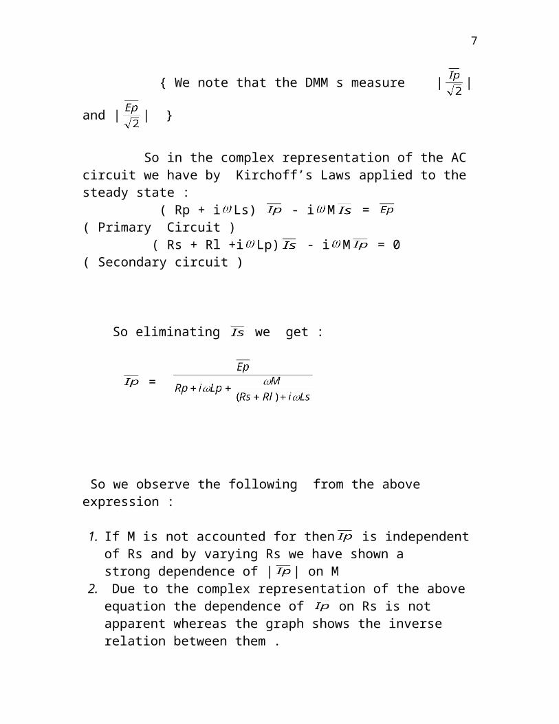
So eliminating we get :

=

So we observe the following from the above expression :

1. If M is not accounted for then is independent of Rs and by varying Rs we have shown a strong dependence of | | on M

2. Due to the complex representation of the above equation the dependence of on Rs is not apparent whereas the graph shows the inverse relation between them .

3. The term is called the “ Reflected Impedance “

4. If the secondary is open i.e (Rs + Rl) = then the primary current is determined by the parameters of the primary circuit alone ie

=

5. If the secondary is shorted i.e ( Rs+ Rl) 0 then we shall have

=

7

6 . As a further special case of the above if we consider that as in an ideal case M = K (LsLp) and that K = 1 then we have : =

8

3. Part B

a) The experimental set-up and the circuit details… The circuit diagram is as follows :

where 1. E0 = the potential across the terminals of the

step down transformer which steps down from 220 V (approx.) A.C mains to 7.4 V (approx.)

2. Ip , Il , Ir = the RM.S values of the steady state currents in the primary circuit and left and the right secondary respectively.

3. Rp , Rl , Rr = the lumped resistances of the primary circuit and the left and the

right secondary respectively.4. Lp , Ll , Lr = the self inductances of the primary

circuit and the left and the right secondary respectively.

5. Ml , Mr = the mutual inductances between the left coil and the primary coil and between the right coil and the primary coil respectively .

6. Ep , El , Er = the potential difference across the coils in the primary , left and the right secondary respectively.

9

b ) Certain Observations About The Procedure Of This Experiment

1. We neglect any mutual inductance between the coils of the left and the right secondaries.

2. Because of the very geometry of the transformer we find it difficult to measure the flux linkage through any coil.

3. Due to the above mentioned constraint we measure/observe 3 other parameters of sny of the arms as and when which is found to be more easy or useful. i.e

a) the current in that arm of the circuit . b) potential drop across a coil or a resistance . c) or qualitatively estimate by observing the glow of the bulb in the left arm.

4. We necessarily observe that in this experiment the number of parameters is > 2 ( the number of independent variables is already = 2 i.e Rl and Rs ) hence the dependencies are very high dimensional . So to be able to demonstrate the dependencies well we have 2 alternatives :

a) We plot 3 dimensional plots to show the dependencies on the 2 independent variables.

b) We take our independent variables in such combinations (by keeping either of them constant) that we can pick out pairs of interdependent parameters to plot and hence effectively take projections in our very high dimensional parameter space.

2. We assume the 2 sides of the primary coil to be symmetrical and the 2 coils (each of 300 turns of 23 SWG wires ) of the left an the right secondaries to be

10

identical . We assume this symmetry in the circuit and assume that if the circuit conditions in the left and the right interchanged then the results would be identical . So we create out parameters on either side depending on when which is found convenient.

c) The Observation Tables

We vary the load resistances in the left and the right secondary and measure the parameters Ep ( in the sense as specified in the brackets above ) ,El , Er , Ip , Il and Ir For each of the configurations.

i) Both The Secondaries Have Finite Resistances (With One Constant)

Rr (Ohms)

Rl (Ohms)

El ( Volts)

Ep (Volts)

Er (Volts)

Il (Amperes)

Ip (Amperes)

Ir (Amperes)

1.3 1.2 2.28 6.17 2.27 2.000 2.000 1.98

1.3 2.1 1.96 6.30 3.3 1.486 1.474 1.455

1.3 2.4 1.844 6.34 3.55 1.38 1.374 1.35

1.3 3.5 1.545 6.50 4.2 1.164 1.155 1.127

1.3 5.1 1.250 6.67 4.82 0.943 0.938 0.905

1.3 6.0 1.117 6.73 5.10 0.845 0.838 0.806

1.3 7.3 0.974 6.79 5.37 0.735 0.733 0.696

1.3 8.0 0.824 6.79 5.59 0.608 0.602 0.577

1.3 8.9 0.779 6.80 5.66 0.574 0.58 0.528

1.3 10.6 0.670 6.90 5.9 0.500 0.500 0.475

1.3 15.6 0.515 7.01 6.23 0.381 0.39 0.341

11

1.3 18.4 0.448 7.02 6.33 0.337 0.344 0.291

1.3 22.6 0.364 6.93 6.3 0.36 0.272 0.234

1.3 27.0 0.317 7.09 6.62 0.244 0.244 0.144

ii) The Left Secondary is shorted ( Rl 0 )

Rr (Ohms) Rl (Ohms) El ( Volts) Ep (Volts) Er (Volts)Il (Amperes)

Ip (Amperes)

Ir (Amperes)

0 1.2 0.1864 5.93 3.17 2.92 2.86 2.84

0 2.1 0.143 6.12 4.22 2.2 2.21 2.17

0 2.4 0.437 5.98 4.29 1.725 1.705 1.662

0 3.5 0.333 6.02 4.76 1.347 1.327 1.291

0 5.1 0.273 6.51 5.55 1.104 1.09 1.054

0 6.0 0.242 6.61 5.77 0.976 0.962 0.924

0 7.3 0.209 6.68 5.96 0.839 0.83 0.79

0 8.0 0.191 6.66 5.98 0.772 0.764 0.725

0 8.9 0.178 6.73 6.09 0.715 0.708 0.668

0 10.6 0.154 6.77 6.1 0.623 0.617 0.575

0 15.6 0.114 6.93 6.51 0.454 0.45 0.407

12

0 18.4 0.0979 6.97 6.54 0.396 0.395 0.35

0 22.6 0.0833 6.99 6.63 0.338 0.338 0.291

0 27.0 0.0721 7.04 6.63 0.293 0.294 0.245

0 50.7 0.1974 6.97 6.73 0.1737 0.1804 0.1283

0 99.5 0.1334 7.02 6.83 0.1174 0.1249 0.0672

iii) The Left Secondary Is Open ( Rl )

Rr (Ohms)

Rl (Ohms)

El ( Volts)

Ep (Volts)

Er (Volts)

Il (Amperes)

Ip (Amperes)

Ir (Amperes)

infinity 1.2 6.92 7.15 0.1389 0 0.0715 0.0628

infinity 2.1 6.85 7.11 0.1884 0 0.0712 0.0619

infinity 2.4 6.83 7.12 0.214 0 0.0709 0.0615

infinity 3.5 6.77 7.10 0.276 0 0.0702 0.0604

infinity 5.1 6.70 7.1 0.362 0 0.0695 0.0590

infinity 6.0 6.64 7.09 0.413 0 0.0689 0.0579

infinity 7.3 6.54 7.04 0.479 0 0.0685 0.0568

infinity 8.0 6.54 7.06 0.511 0 0.0683 0.0563

infinity 8.9 6.51 7.05 0.558 0 0.0675 0.0553

infinity 10.6 6.45 7.07 0.631 0 0.0669 0.0541

13

infinity 15.6 6.28 7.09 0.846 0 0.0651 0.0502

infinity 18.4 6.2 7.12 0.955 0 0.0640 0.0483

infinity 22.6 6.05 7.08 1.09 0 0.0629 0.0461

infinity 27.0 5.93 7.11 1.229 0 0.0614 0.0435

infinity 50.7 5.4 7.1 1.765 0 0.0569 0.0338

d) Analysis Of The Graphs To Determine The Qualitative Behaviour.

I) Both Secondaries Have Finite Non Zero Resistances

i) Behaviour of the currents when both the secondaries have finite resistances

a) The graph of Il vs Rr :

14

We can easily infer from the above graph that Il is(non-linear) inversely proportional to Rr and Il undergoes a slight rise and fall after 15 Ohms

15

b) The graph of Ip vs Rr

We can infer from the above graph that Ip is (non-linear) inversely proportional to Rr

c) The graph of Ir vs Rr

16

We can infer from the above graph that Ir is (non-linear)inversely proportional to Rr

ii) Behaviour of the potential differences when both the secondaries have finite resistances

a) The graph of El vs Rr

We can infer from the graph that El is (non-linear) inversely proportional to Rr

b) The graph of Ep vs Rr

17

We can infer from the graph that Ep is (non-linear) directly proportional to Rr.

and it undergoes a slight fall and rise after around 20 ohms.

c) The graph of Er vs Rr

18

We can infer from this graph that Er is (non-linear) inversely proportional to Rrand it undergoes a slight fall and rise from around 20 ohms.

d) The graph of Er vs Ir

We can infer from the above graph that Er is (non-linear) directly proportional to Ir and undergoes a slight fall and rise from around 20 ohms.

19

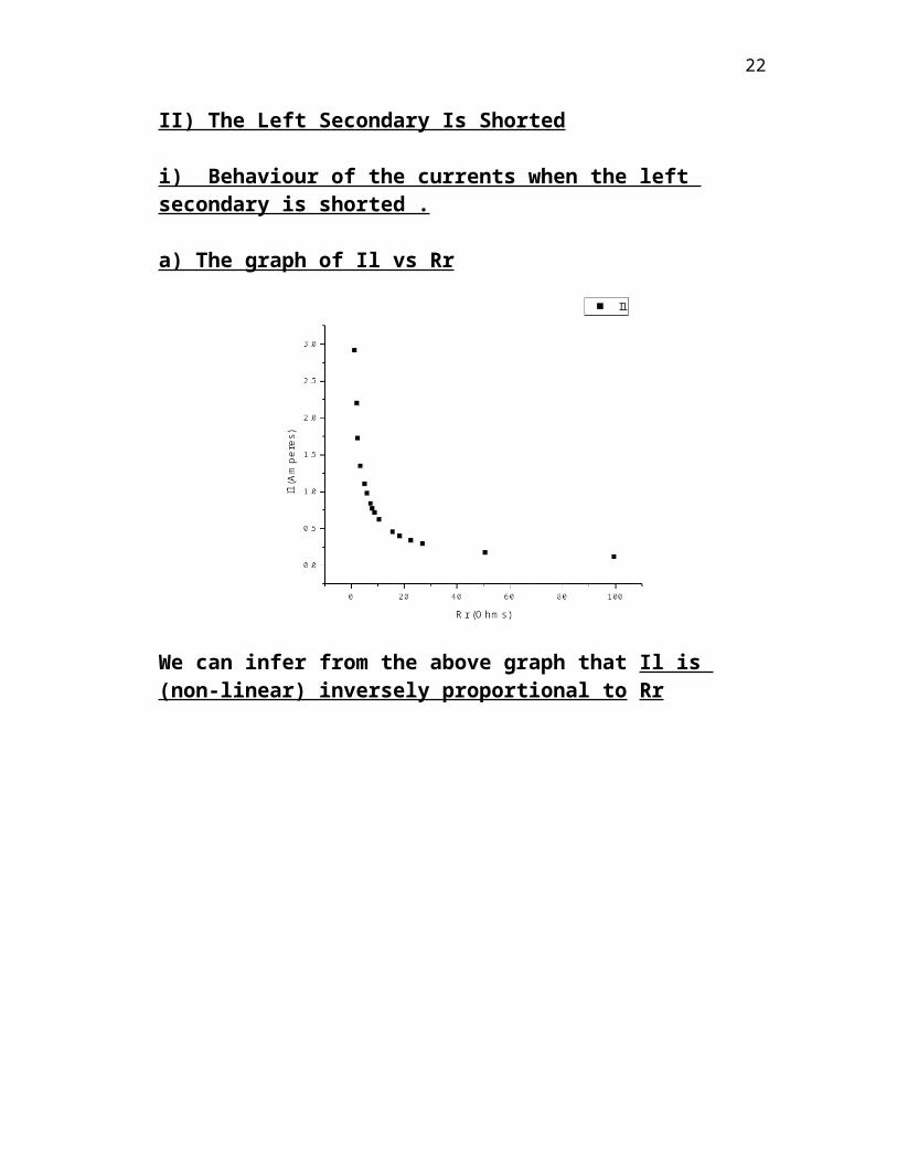
II) The Left Secondary Is Shorted

i) Behaviour of the currents when the left secondary is shorted .

a) The graph of Il vs Rr

We can infer from the above graph that Il is (non-linear) inversely proportional to Rr

20

b) The graph of Ip vs Rr

We can infer from the above graph that Ip is (non-linear) inversely proportional to Rr

c) The graph of Ir vs Rr

We camn infer from the above graph that Ir is (non-linear) inversely proportional to Rr

21

ii) Behaviour of the potentials when the left secondary is shorted.

a) The graph of El vs Rr

We can infer from the above graph that El is ( non-linear ) inversely proportional to Rr and it undergoes a rise and fall in the approximate ranges 1 to 2.5 ohms and after around 27 ohms.

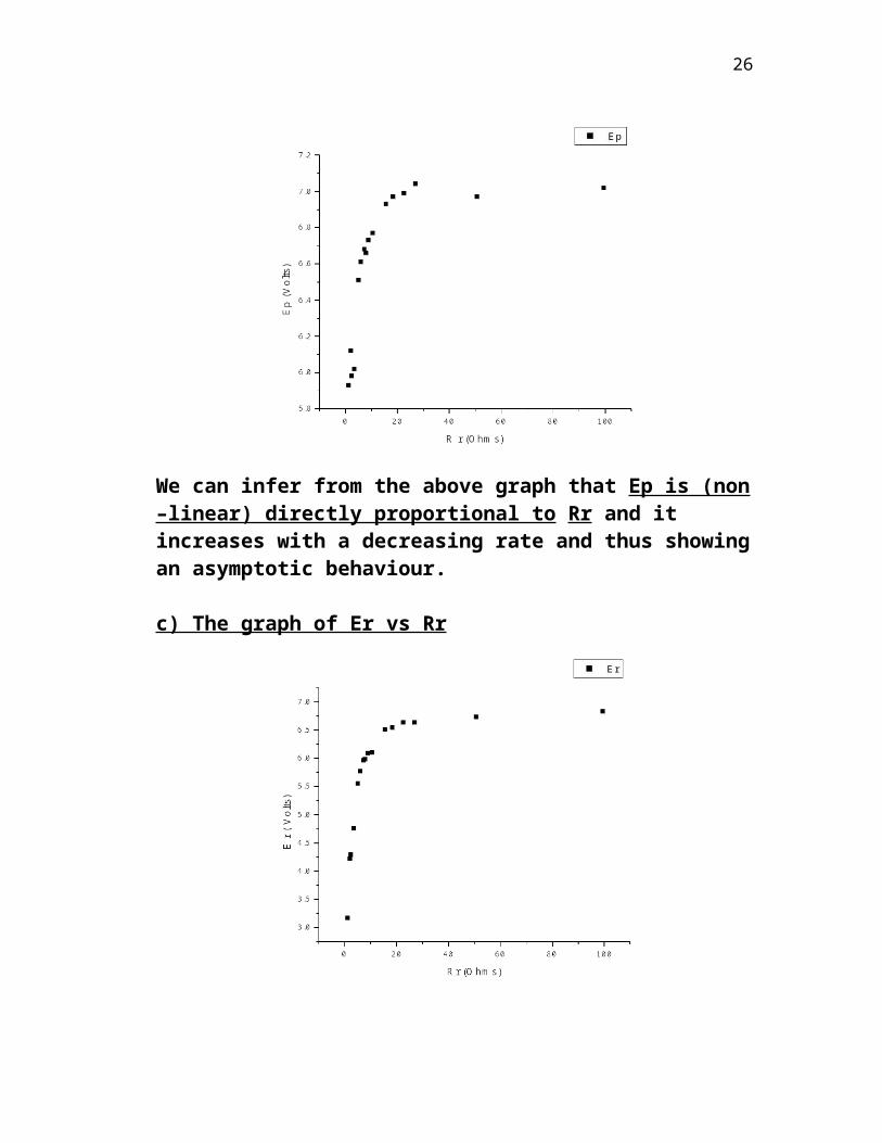
b) The graph of Ep vs Rr

22

We can infer from the above graph that Ep is (non –linear) directly proportional to Rr and it increases with a decreasing rate and thus showing an asymptotic behaviour.

c) The graph of Er vs Rr

We can infer from the above graph that Er is (non –linear) directly proportional to Rr and it increases

23

with a decreasing rate and thus showing an asymptotic behaviour.

24

III) The Left Secondary Is Open

i) Behaviour of the currents when the left secondary is open .

a) The graph of Ip vs Rr

We can infer from the above graph that Ip is inversely proportional to RrAnd the dependency is almost linear

b) The graph of Ir vs Rr

25

We can infer from the above graph that Ir is inversely proportional to Rrand the dependency is almost linear.

ii) Behaviour of the potentials when the left secondary is open.

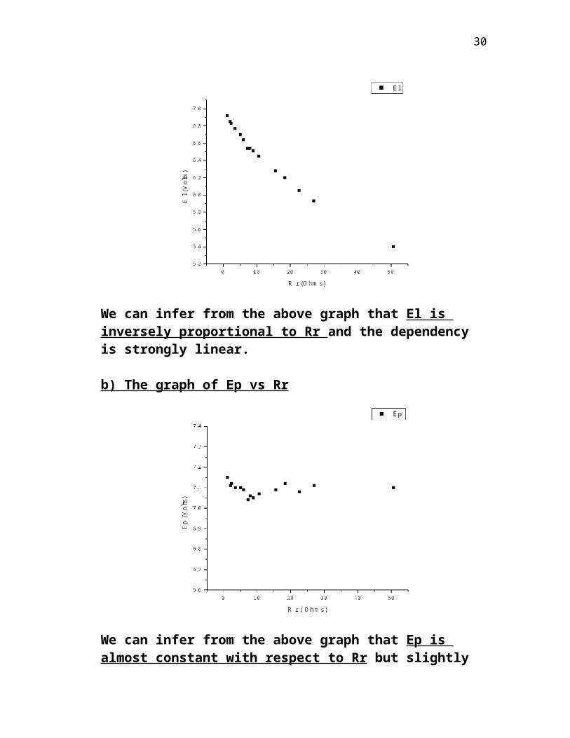
a) The graph of El vs Rr

26

We can infer from the above graph that El is inversely proportional to Rr and the dependency is strongly linear.

b) The graph of Ep vs Rr

We can infer from the above graph that Ep is almost constant with respect to Rr but slightly oscillating around a mean value of 7.1 V which is slightly lower than the potential across the transformer.

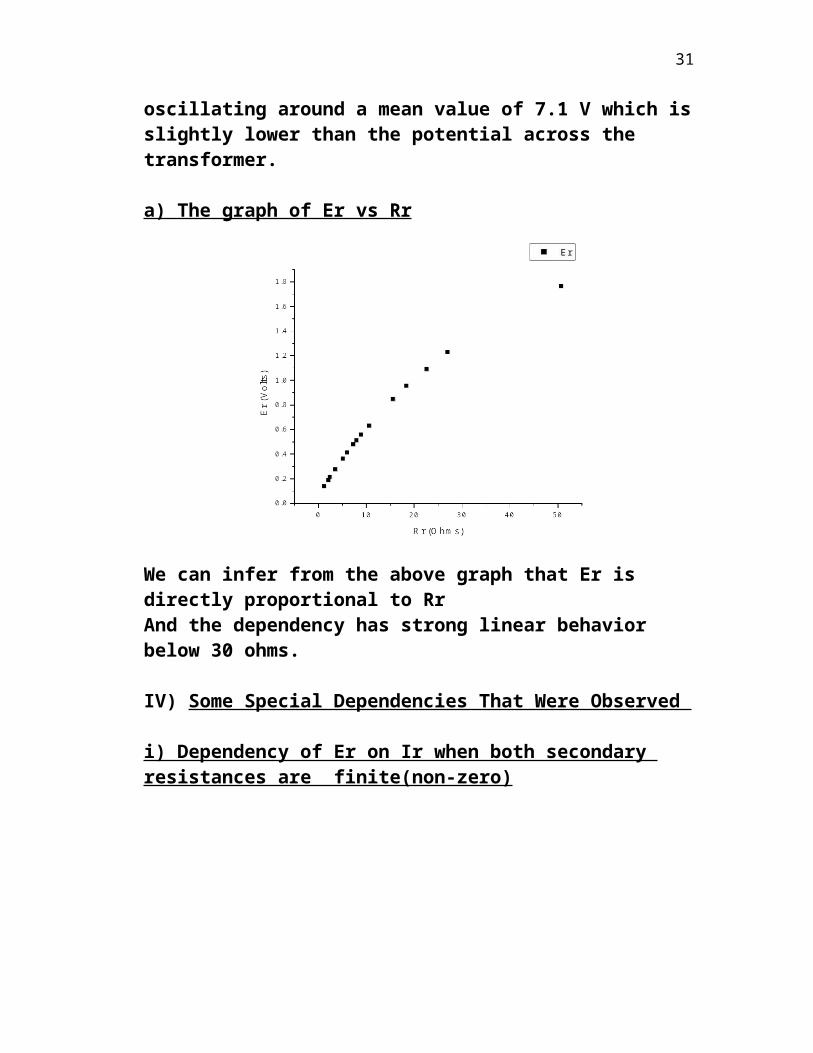
a) The graph of Er vs Rr

27

We can infer from the above graph that Er is directly proportional to RrAnd the dependency has strong linear behavior below 30 ohms.

IV) Some Special Dependencies That Were Observed

i) Dependency of Er on Ir when both secondary resistances are finite(non-zero)

28

We observe that Er is non-linearly and directly proportional to Ir and though it shows a slight rise and fall at around 20 – 30 ohms we might expect it to have an asymptotic behaviour.

This also indicates from its slope that the magnitude of the impedance of the right secondary is also increasing sharply with increase of its current.

ii) Dependency of Er on Ir when the left secondary is open.

29

We observe from the above graph that Er is inversely related to Ir when the left secondary is open ( exactly reverse behaviour from previous case when the left secondary had a finite non zero resistance ).

Secondly this dependency is strongly linear whereas the previous case was highly non-linear.

Thirdly from the slope of the graph we have the unavoidable conclusion that it shows a negative value of the magnitude of impedance (!)

iii) Dependency of Impedance of the primary on the resistances of either of the secondaries.

We see that the value of is equal to the effective A.C resistance or Impedance of the primary which we denote as Zp. In the following we observe some interesting dependencies of Zp on the values of the load resistances in the secondaries.

30

31

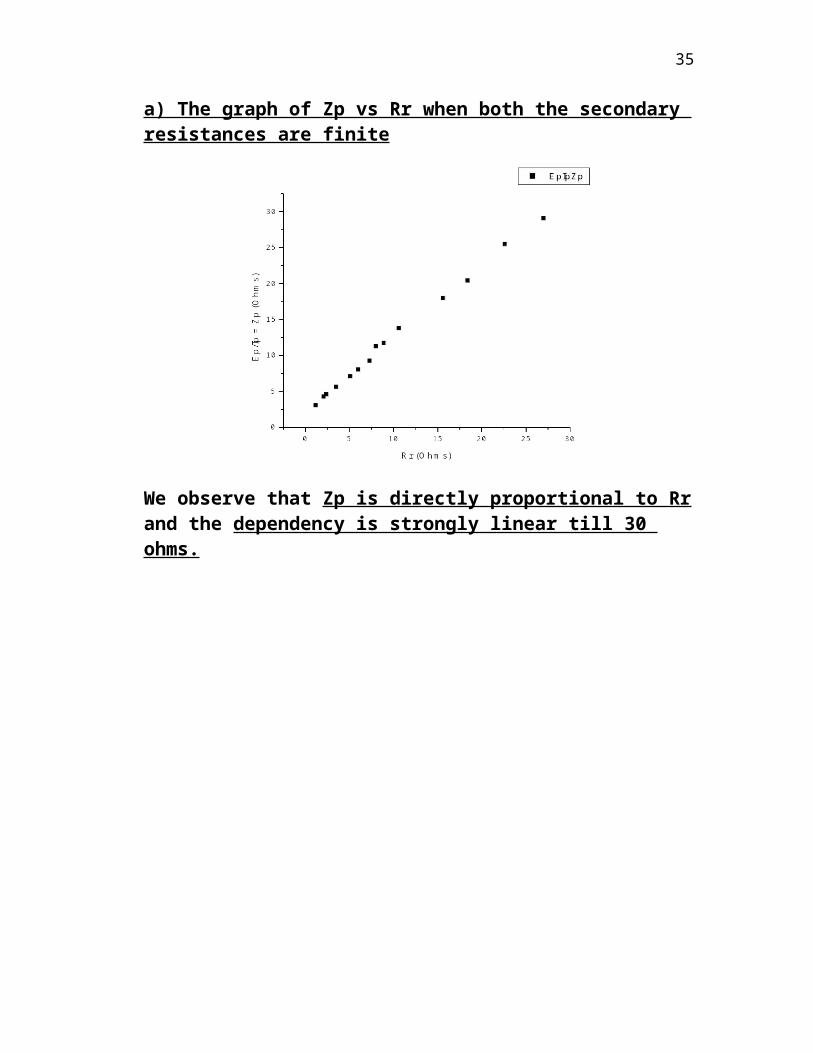
a) The graph of Zp vs Rr when both the secondary resistances are finite

We observe that Zp is directly proportional to Rr and the dependency is strongly linear till 30 ohms.

32

We observe that Zp is directly proportional to Rr and the dependency is strongly linear till 30 ohms .

c) The graph of Zp vs Rr when the left secondary is open.

We observe that Zp is directly proportional to Rr and the dependency is strongly linear till 30 ohms.

33

e)Theoretical Analysis Of This Experiment

i) The experimenter’s observations regarding the procedure of the experiment have been already put down in section 3)Part B (b) .

ii) Theoretical Analysis Of The Experiment

The Basic Theory Of Transformer :

The maxwell’s law about the curl of the electric field states that the curl of the electric field in an infinitesimal region is equal to the negative of the parial derivative of the magnetic field at that region at that instant. This law when surface integrated and surface integral of the curl of the electric field converted to line integral of the field along the circuit loop involved in the secondary coil tell us that that a potential difference will be generated across the secondary as the flux of the magnetic field through it is changing with time since the current passing in the primary i.e the current causing the magnetic field in the secondary coil is AC . Hence a potential is generated across the secondary whose magnitude depends on the coupling between the primary and the secondary coils which in turn depends on the relative geometries as is reflected in the Neumann integral taken over these 2 coils .

In order to avoid the complex differential equations that a

dynamic analysis of time evolution of the circuit will involve we look at the approximate steady state analysis

of the flux distribution of the primary coil among the 2 secondary coils.

34

We assume for theoretical ease that the magnetic permeability of the laminated core of the conductor is sufficiently high to contain the total flux produced and there is no loss of flux out of the transformer .

Let p be the flux through the primary coil of the

transformer and let l and r be the flux through the left and the right secondary coils. Therefore from the above assumption we get p = l + r.

We note that that p , l, r are all due to the self inductance of the respective coils and mutual inductances ( ignoring mutual inductance between the 2 secondaries ).

We also observe that the potential differences and the current measured are a reflection of the time variation of the ’s . But as the time intervals considered are the same for all ultimately the measurements indicate how is p distributed among l and r .

We consider the following special cases to get a qualitative feel of the situation :

i) Both Secondaries Are Open ( Rr = Rl ) Here we have Rr = Rl and we expect the current in the primary to behave as if there are no secopndaries and hence determined by the parameters of the primary alone. Let Np , Nl and Nr be the number of turns in the primary and the left and the right secondaries . Here we note that there will exist a El and an Er but no Il or Ir .So we have the following equations : Ep = - Np , = +

By symmetry we have l = r and Np = Nl = Nr and hence Er = El = - Nl = - Nr =

35

i.e Er = El =

ii) Both Secondaries Are Shorted ( Rr = Rl 0 ) Since the geometries of the 3 arms of the transformer are equal we expect their inductances to follow the following equations :Ll = CNl2 , Lr = CNr2 and Mr = k = kCNpNr and similarly Ml = kCNpNl

Where C is a constant which depends on the inherent geometries of the coils and hence equal for both the left and the right coils . k is the coupling constant between the primary and the secondary and by symmetry is the same for both . Now invoking the fact that Np = Nl = Nr we get Mp = Mr = Ll = Lr and let Mp = Mr be = M and Ll = Lr = L .So when the above equality conditions are invoked in the steady-state’s maximal current equations along with the fact that Rr = Rl 0 we get :

i MIp = i LIl and i MIp = i Lir

and hence the conclusion that Il = Ir = Ip .

Further due to the above equations we also get that there will be ideally no net flux intercepted through either of the secondaries and hence no potential differences across them and by the equation p = l + r we get that there will be no flux through the primary as well .As a result the effective impedance of the primary is greatly reduced and hence the primary current is very high .

iii) Extreme Asymmetric Loading ( Rl and Rr 0 ) Here the Ir is not limited by any load resistance and it will be ideally of such value so that the magnetic flux it produces almost completely negates the flux produced by mutual induction from the primary i.e ideally

36

MIp = LIr So r = 0 and hence Er = - Nr = 0 . Further p = l + r and hence p = l. Therefore taking the time derivative and since Np = Nl we get Ep = El .and we already have Er = 0 . And since M = L we get Ip = Ir .

37

iv) Both Secondaries Have Equal Resistances We note that the three legged core of the transformer is symmetrically fabricated ( with respect to the number of turns of the wire , the wire type and dimensions ) hence the values of Lp , Ll , Lr are equal and and also Ml = Mr for similar reasons . Hence with symmetric loading the circuit is expected not to differentiate between the two sides and we have p = l + r , and l = r and hence l = r = p/2 and

hence we expect their time derivatives to be also equal and hence El = Er = and Il = Ir .

V) Any Combination Of Values Of Rr And Rl From a theoretical standpoint this is the most important case as the behaviour of the circuit is characterized by its response to this range of finite values . Here the theoretical analysis is very complex for the dynamic time evolution of the circuit but the steady state values can be estimated by the solutions of the 3 variables Ip , Il , Ir for a given value of Rr , , Rl and Eo of the following approximate equations in the complex number representation :

Rp + i ( M( + ) - L ) = Rl + i (M - L ) = 0 Rr + i ( M - L ) = 0

38

{ This equations other than being approximate in neglecting the very small transient component of the steady state current are also assuming resistances of the wires to be = 0 and hence we should ideally have the potential across the transformer to be equal to the potential across the primary but in practice this assumption is not found to be true always as shown in the readings of section (e) }

Hence to overcome these above cited difficulties we resort to experimental results to be able to atleast qualitatively gauge the mode of dependency of the currents and the potential drops on the Rr and Rs from the graphs .

Here we more clearly see the need to do the measurements by varying only one of Rr or Rl at a time so that the individual dependencies of the complex solutions can be gauged.

39

iii) Theoretical Analysis Of Some Of The Precautions In This Experiment { The explanations are with respect to the configuration of Part A with the addition of a bulb in the primary circuit

}

a) If secondary is shorted

If the secondary circuit is completed then the resistance in it will be very low and it will allow a high current to pass through it and its maximal value will increase till the net flux through through it becomes equal to 0.

The current flowing in the secondary will cause a time variant flux to be induced in the primary (mutual induction ) and then the current in the primary will also increase to nullify this change . Hence a high current will flow in the primary making the attached bulb glow brighter .

The process will equilibriate (i.e the maximal values of the sinusoidal variations will stabilize ) when the flux linkage in the secondary becomes 0 and the flux linkage is restored to its original values . (final maxima of the currents will be solutuions of 2 simultaneous equations )

b) Effect of shorting the secondary on the impedance of the primary

The phenomenon of mutual inductance makes

the current in the primary dependent on the current in the secondary and hence by shorting the secondary or making any change in the secondary changes the impedance ( or the effective resistance in an A.C circuit ) .The dependence is strong if the coupling constant is near to 1 as it is in this experiment.

40

c) If turns If the number in the secondary coil is is increased

Increasing the number of turns in the secondary

will increase the flux linked through it and the potential induced across it proportionately ( if current is not allowed to flow through the secondary ) if it is done without affecting the relative geometries between the coils i.e the coupling constants remain remain near to 1 even after the change .

A higher potential induced in the secondary will trigger the same response as explained in b) and will cause a huge current to flow in the primary and this may cause burning or damaging of the components in the primary if it goes beyond its tolerance limit.

d) The precaution that results from the above discussions

The explanation b) and c) together indicate that we must not allow high current to flow through the secondary for the safety of components connected t0 the primary.

But if flux linkage through the secondary increases (either due to changes in the primary or due to effects as in c) or effects in ans b) nature will take its own course to increase the flux linkage of the opposite sign to negate the effect . So that nature does it not at the expense of passing more current we must use the coils of high inductance so that current in the secondary is kept low . This will be able to prevent the sudden rise of current in the primary since that can increase only due to mutual induction which here will only depend on the secondary current .

Overall we must avoid shorting the secondary.

41

iv) The Sources Of Errors And Their Remedies Suggested/Adopted

i) The DMM shows arbitary fluctuations and at times the amplitude is about 1 V or 1 A . To glean the truth out of such situations we have adopted the following measures :

a) Instead of the DMM probes banana clips were used

so that the fluctuation caused due to the movement of the contact point of the pin head probe and the large socket is reduced .

b) Attempt was made to reduce disturbances in the circuit due to movement of the wires as minimum as possible.

c) The rust on the sockets could also have caused the readings to fluctuate frantically and so it is suggested to use sockets of stainless steel

d) The mean value of the fluctuations has been taken as the data

ii) The resistors heat up very fast and causing thus making the current drop at times by around 1.5 A per 7 min . To counter this the following things were done :

a) 6 DMM’s were used in the second try of the experiment to be able to take the measurements of the 6 parameters simultaneously ( initially due to insufficient DMM’s error due to continual change of circuit was huge) . Further this reduces time for which current has to continually pass through the circuit and hence prevents heating up.

b) Power was turned off in between circuit rearrangements.

42

c) Measurements were tried to be noted down within 1 min to reduce the time for which current passes.

d) The process of taking the mean of the readings was used to get quality data.

iii) In the attempt to reduce the time for which current had to be passed continually there could have been some minor errors in not allowing the circuit to reach the steady state after the transient components become negligible.

iv) The magnetic fields of the transformer in the 3 arm case are not well contained and hence was a fairly good amount of time variant magnetic field around it producing a potential difference of about .3 to .4 V in the atmosphere near it . Presence of this magnetic field was causing unwanted induction effects in the adjoining parts of the circuits . (especially the crocodile clips ) . This induction effect introduced caused a spatial dependence of the resistance of the circuit elements . To minimize this attempt was made to keep the movement of the circuit linkages as low as possible and positions as constant as possible during the process of reading the data. 2 remedies can be suggested here :

a) The transformer can be made of better layering by reduction of gaps and by using material of higher magnetic permeability.

b) To create some magnetic shield around the transformer)

43

44

f) Experimental Test Of Some Of The Special Cases

1. Let a bulb be attached to the left secondary.We observe that the bulb glows when the right secondary is complete and not when the right secondary is open although there is no electrical connection between them. As explained in Part B section e (ii) (iii) when one of the secondaries is shorted the entire flux of the primary links to the other secondary whereas when both of the secondaries have resistances ( may be infinite when open as here ) the flux distributes itself in some proportion and hence the flux linkage is less than when it is shorted . And potential drop across the bulb is proportional to the flux linkage in the coil to which it is connected . Hence the above observation is explained.

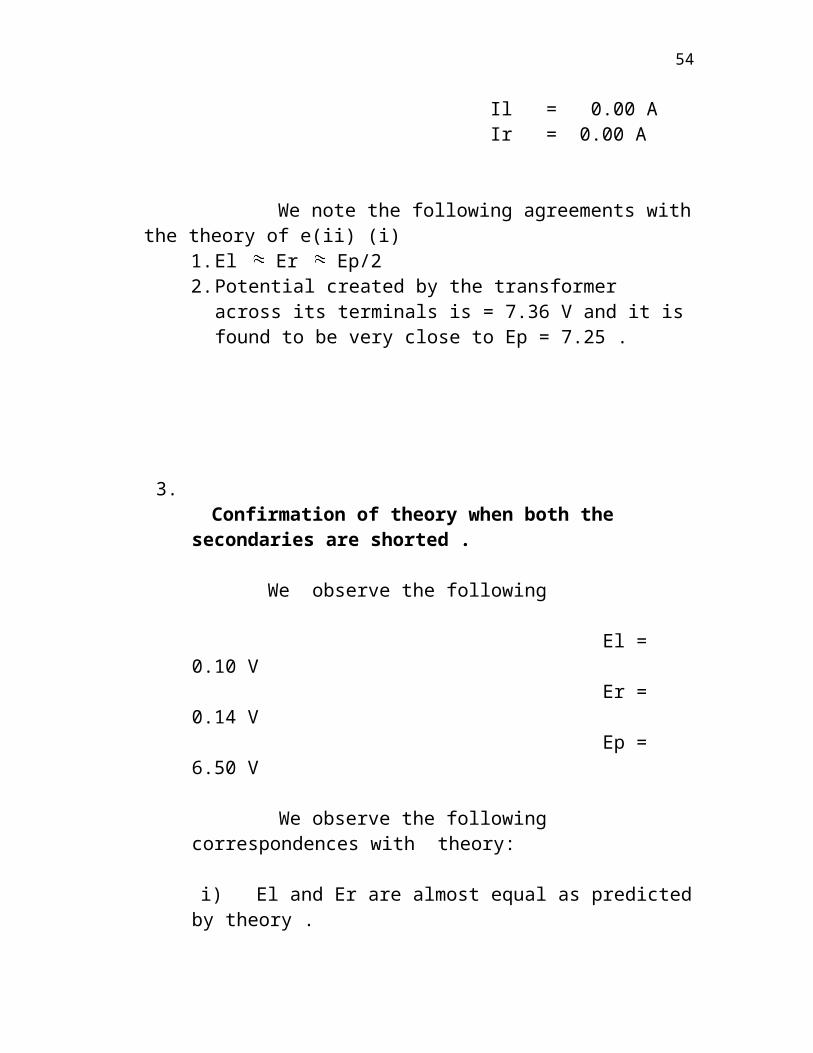
2. Confirmation of theory when both the secondaries are open. We make the following observations in this case : Ep = 7.25 V El = 3.58 V Er = 3.52 V Ip = 0.02 A Il = 0.00 A Ir = 0.00 A

We note the following agreements with the theory of e(ii) (i)

1. El Er Ep/22. Potential created by the transformer across its

terminals is = 7.36 V and it is found to be very close to Ep = 7.25 .

45

3. Confirmation of theory when both the

secondaries are shorted . We observe the following El = 0.10 V Er = 0.14 V Ep = 6.50 V

We observe the following correspondences with theory:

i) El and Er are almost equal as predicted by theory . ii) Potential across the transformer is not equal to Ep 4. Confirmation of theory in the case of asymmetric loading We set Rl and Rr 0 and we make the following observations Ep = 7.25 V El = 7.20 V Er = 0.00 V Il = 0.01 A Ir = 0.05 A Ip = 0.05 A

We observe the following correlations with the theory of e(ii) (iii)

1. Ep and El are almost equal as predicted in theory (deviation of 0.69 %)

46

2. Ip and Ir are equal as predicted by theory .3. Er is equal to 0 as predicted .4. Ep and ( El + Er ) are almost equal as predicted

by theory (deviation of 0.69%)

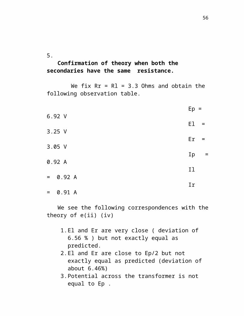
5.Confirmation of theory when both the

secondaries have the same resistance.

We fix Rr = Rl = 3.3 Ohms and obtain the following observation table.

Ep = 6.92 V El = 3.25 V Er = 3.05 V Ip = 0.92 A Il = 0.92 A Ir = 0.91 A

We see the following correspondences with the theory of e(ii) (iv)

1. El and Er are very close ( deviation of 6.56 % ) but not exactly equal as predicted.

2. El and Er are close to Ep/2 but not exactly equal as predicted (deviation of about 6.46%)

3. Potential across the transformer is not equal to Ep .

We note from the comparison of values of Ep and Eo that only when the secondaries are in extreme asymmetric loading or both open state the

47

resistance of the wires of the primary circuit can be neglected and otherwise not.

48

49

50

51

52

53

54

55

56

57