an examination of the nature of global modis cloud regimes · an examination of the nature of...

An examination of the nature of globalMODIS cloud regimesLazaros Oreopoulos1, Nayeong Cho1,2, Dongmin Lee1,3, Seiji Kato4, and George J. Huffman1

1NASA-GSFC, Earth Science Division, Greenbelt, Maryland, USA, 2USRA, Columbia, Maryland, USA, 3GESTAR, Morgan StateUniversity, Baltimore, Maryland, USA, 4NASA-LARC, Climate Science Branch, Hampton, Virginia, USA

Abstract We introduce global cloud regimes (previously also referred to as “weather states”) derivedfrom cloud retrievals that use measurements by the Moderate Resolution Imaging Spectroradiometer(MODIS) instrument aboard the Aqua and Terra satellites. The regimes are obtained by applying clusteringanalysis on joint histograms of retrieved cloud top pressure and cloud optical thickness. By employing acompositing approach on data sets from satellites and other sources, we examine regime structural andthermodynamical characteristics. We establish that the MODIS cloud regimes tend to form in distinctdynamical and thermodynamical environments and have diverse profiles of cloud fraction and water content.When compositing radiative fluxes from the Clouds and the Earth’s Radiant Energy System instrument andsurface precipitation from the Global Precipitation Climatology Project, we find that regimes with a radiativewarming effect on the atmosphere also produce the largest implied latent heat. Taken as a whole, the results ofthe study corroborate the usefulness of the cloud regime concept, reaffirm the fundamental nature of theregimes as appropriate building blocks for cloud system classification, clarify their association with standardcloud types, and underscore their distinct radiative and hydrological signatures.

1. Introduction

The role of clouds in the Earth’s water and energy cycle cannot be overstated. Atmospheric heating rates(due to radiative and phase change processes), surface energy budgets (radiative and turbulent), andprecipitation rates depend strongly on cloud coverage, optical and microphysical properties, and frequency ofoccurrence. Cloud impacts are often studied either collectively or by employing only rudimentary classification,e.g., based on phase (liquid and ice clouds) or height (low, middle, and high clouds). However, as we willshow here, a moremethodical categorization of the multitude of observed cloud systems can potentially be farmore useful and serve as a springboard of advanced physically based diagnostics to evaluate cloud processesin global climate model (GCM) simulations.

There has recently been a proliferation of studies focusing on the subject of systematic identification of distinctcloud regimes via extraction of patterns in the covariation of cloud vertical location and extinction. Acommon practice is to deduce the patterns using clustering techniques [Jakob and Tselioudis, 2003; Rossowet al., 2005; Zhang et al., 2007]. The search for patterns can be performed on either discrete geographicalregions or climatic zones [e.g., Jakob and Tselioudis, 2003; Haynes et al., 2011; Oreopoulos and Rossow, 2011;Tan and Jakob, 2013] or encompass global scales [Tselioudis et al., 2013]. Once the regimes have beenidentified, major features such as frequency of occurrence and distributions of cloud fraction, top and baseheight, vertical structure, optical properties, etc., can be inferred, depending on the availability of coincidentobservations. These features can in turn serve as the basis for more advanced analysis such as evaluation ofcloud regime role in weather and climate processes.

One of the earlier works embracing the cloud regime concept was that by Jakob et al. [2005]. The authorsinvestigated the radiative (surface and top of the atmosphere (TOA) fluxes), cloud property (profiles of cloudfraction, joint variations of cloud height, and vertical extent), thermodynamical (columnar water vapor,temperature profiles), and dynamical (vertical velocities) characteristics of International Satellite CloudClimatology Project (ISCCP) cloud regimes in the western Pacific in order to better understand the role ofclouds on regional water and energy budgets. Later, Jakob and Schumacher [2008] brought in precipitationand latent heating data from the Tropical Rainfall Measuring Mission precipitation radar in the same region tosuccessfully associate cloud regimes with three major precipitation regimes of distinct rainfall rates andlatent heat profile characteristics. Gordon and Norris [2010] investigated whether particular midlatitude

OREOPOULOS ET AL. ©2014. American Geophysical Union. All Rights Reserved. 1

PUBLICATIONSJournal of Geophysical Research: Atmospheres

RESEARCH ARTICLE10.1002/2013JD021409

Key Points:• Cloud systems observed by passivesensors can be decomposed intocloud regimes

• The regimes have distinct structuresas seen by active sensors

• The regimes also have distinctradiative and hydrological signatures

Correspondence to:L. Oreopoulos,[email protected]

Citation:Oreopoulos, L., N. Cho, D. Lee, S. Kato,and G. J. Huffman (2014), An examinationof the nature of global MODIS cloudregimes, J. Geophys. Res. Atmos., 119,doi:10.1002/2013JD021409.

Received 20 DEC 2013Accepted 21 JUN 2014Accepted article online 27 JUN 2014

https://ntrs.nasa.gov/search.jsp?R=20140013289 2020-04-06T06:05:00+00:00Z

oceanic cloud regimes, as derived by their own in-house cluster analysis of ISCCP cloud optical thicknessand cloud top pressure 2-D histograms, were associated with systematic deviations from the meanatmospheric state as represented by reanalysis fields of relative humidity, temperature, vertical velocity,and horizontal temperature advection.

The ISCCP project has been providing for a few years now its own cloud regime (“weather state,” in theirterminology) product based on application of a k-means clustering algorithm [Anderberg, 1973] on cloudoptical thickness–cloud top pressure 3 h joint histograms of 2.5° gridcells (http://isccp.giss.nasa.gov/climanal5.html). The initial edition of the data set was available only for the deep tropics (15°S to 15°N)[Rossow et al., 2005] but was subsequently expanded to cover three distinct geographical zones (extendedtropics, 35°S to 35°N, and northern and southern midlatitudes between 30° and 65°). Compositing radiativeflux and precipitation data by ISCCP weather state led to insight on their hydrological and radiative nature[Haynes et al., 2011; Oreopoulos and Rossow, 2011; Lee et al., 2013; Rossow et al., 2013] and, in particular, to abetter understanding of their individual importance to the water and energy budget as measured bycontribution strength. At the same time, parallel efforts concentrated on deriving regimes from appropriatelyequipped GCMs, with comparisons to observed regimes and attribution of potential cloud radiativefeedbacks as two notable lines of research [Williams and Tselioudis, 2007; Williams and Webb, 2009]. Othernovel applications have also started to emerge recently such as examination of aerosol indirect effectdependence on regime type and transitions, as recently attempted by Gryspeerdt and Stier [2012] andGryspeerdt et al. [2014] in the tropics using Moderate Resolution Imaging Spectroradiometer (MODIS) data.

Recently, Tselioudis et al. [2013] successfully completed the inexorable last step of deriving a single set ofISCCP weather states for the entire globe. These investigators then used vertical cloud structure informationfrom combined CloudSat-CALIPSO data to deduce the mean vertical layering of weather state cloud fieldsand reanalysis data of vertical pressure velocity to obtain clues about the dynamical environment within whichthey form. Their analysis demonstrated that the vertical layering of the various states is unique and that themean vertical motion of their environment follows an expected progression from intense ascent to gentledescent as one transitions from more to less vertically developed states.

The present paper introduces a new set of global cloud regimes derived by employing clustering analysis on dailyjoint histograms from multiyear passive cloud retrievals by the MODIS instrument aboard the Terra and Aquasatellites. MODIS-based regimes using the same or similar clustering methodology have been derived previously[Williams and Webb, 2009; Lebsock et al., 2010; Gryspeerdt and Stier, 2012; Gryspeerdt et al., 2014], but thisis the first that employs the longest data set available to date and is truly global, which makes it the mostcomparable to its ISCCP counterpart in Tselioudis et al. [2013]. Our goal is twofold: first, to reaffirm that the regimeconcept is as robust as suggested by the prior ISCCP-centric work and can therefore serve as the cornerstonefor cloud system classification in observations and models, and second, to support the notion that othercoincident observations help advance our understanding of the nature of cloud mixtures mapped into regimes.The latter objective becomes particularly important if one wants to determine their distinct hydrological andenergetic characteristics, invaluable information for assessing the realism of cloud simulations in climate models.

2. Data Sources2.1. MODIS Cloud Properties

To derive the MODIS cloud regimes (hereafter CRs, details are forthcoming in section 3.1) we use 10 years(July 2002 to June 2012) of daily Level-3 (D3) 1° ISCCP-like joint histograms of cloud optical thickness (τ)and cloud top pressure (pc) from MODIS-Aqua (MYD08_D3 data set, Collection 5.1) and MODIS-Terra(MOD08_D3, Collection 5.1). The joint histograms are generated from all MODIS pixels for which cloudretrievals are possible and successful, without regard for cloud phase, i.e., pixel count contributions in thesehistograms come from both liquid and ice (and a few undetermined phase) cloud retrievals. Since τ can beretrieved from MODIS measurements only during sunlit hours, the joint histograms are only availableduring daytime. The ISCCP-like MODIS joint histograms originally consisted of seven τ bins and seven pc bins,but we combined the first two τ bins into one (extending from 0 to 1.3) for a total of 42 bins (cf. Figure 1) withthe exact same boundaries (note, however, that for MODIS, the actual upper limit of τ is 100) as those of theISCCP histograms used for that project’s “weather state” analysis [Rossow et al., 2005; Oreopoulos and Rossow,2011; Tselioudis et al., 2013].

Journal of Geophysical Research: Atmospheres 10.1002/2013JD021409


In addition to the joint histograms, for compositing purposes we also use several gridded mean quantitiesavailable in the MODIS D3 data sets. These quantities are the mean cloud fraction and mean τ of successfulcloud retrievals (total, as well as phase-dependent, for both variables). While the phase-agnostic versionsof these variables can also be obtained from the pc-τ joint histogram, we chose for simplicity and forthe purposes of making an independent consistency check to use the mean quantities providedindependently. As will be shown shortly, performing separate compositing for these two variables providesfurther insight into the cloud types (as perceived by passive measurements, at least) that contribute tothe makeup of the MODIS CRs.

2.2. A-Train Data2.2.1. CALIPSO-CloudSat-CERES-MODIS ProductAn enhanced perspective on the nature of cloud regimes can be achieved by employing cloud retrievals fromcoincident active measurements, as sampled, combined, and gridded within the CALIPSO-CloudSat-CERES-MODIS (CCCM or C3M) product [Kato et al., 2010, 2011]. This product was conceived as an aggregator andintegrator of measurements from the Cloud-Aerosol Lidar and Infrared Pathfinder Satellite Observations(CALIPSO) Cloud-Aerosol Lidar with Orthogonal Polarization (CALIOP), CloudSat Cloud Profiling Radar (CPR),

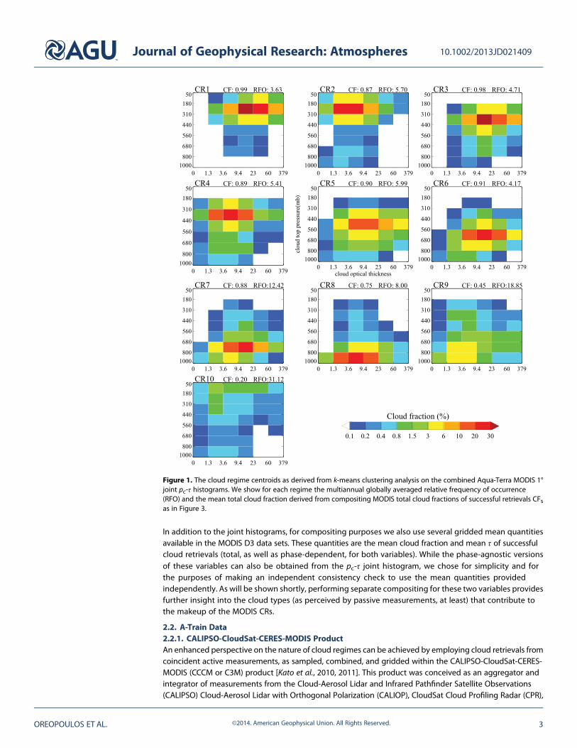
Figure 1. The cloud regime centroids as derived from k-means clustering analysis on the combined Aqua-Terra MODIS 1°joint pc-τ histograms. We show for each regime the multiannual globally averaged relative frequency of occurrence(RFO) and the mean total cloud fraction derived from compositing MODIS total cloud fractions of successful retrievals CFsas in Figure 3.



Clouds and the Earth’s Radiant Energy System (CERES), and MODIS (from the Aqua satellite in the case ofthe latter two instruments). The mapping strategy of C3M is to match cloud and aerosol properties fromCALIOP (nominally resolved at 0.33 km) and cloud properties from the CPR (nominally resolved at 1.4 km) to aMODIS pixel (1 km) and then to the CERES footprint (approximately 20 km) with the highest CALIPSO andCloudSat ground track coverage. Each C3M granule contains 24 h of data, and for the purposes of compositingthe variables of interest by CR, we select only the data subset that falls within 1° D3 gridcells with an AquaCR occurrence for that day.

Our compositing analysis uses 4 years (2007–2010) of C3M data for the following variables: (a) Cloud layertop level height (CCCM-13), the vertical location where the cloud top starts according to combinedCloudSat and CALIPSO retrievals. (b) Cloud layer base level height (CCCM-15), also based on CloudSat andCALIPSO, the vertical location of the first cloud-free layer below a profile’s cloud layer. (c) Cloud fractionprofile (CCCM-52), the volumetric cloud fraction vertical profile derived from CALIPSO and CloudSat data(assigned to CALIPSO bins) and defined as the ratio of CALIPSO cloudy bins within a layer (as delineatedby the radiative transfer model used to obtain irradiance profiles), to the total number of bins withinthe same layer. (d) CloudSat cloud type (CCCM-73), the cloud type according to CloudSat’s 2B-CLDCLASSmask [Sassen and Wang, 2008] provided as the ratio of layers with a given cloud type divided by totalnumber of cloud layers. The CloudSat cloud types are cirrus (Ci), altostratus (As), altocumulus (Ac), stratus(St), stratocumulus (Sc), cumulus (Cu), nimbostratus (Ns), and deep convective clouds (Cb). In practice, theSt cloud type, as defined by the 2B-CLDCLASS, occurs very rarely. (e) Liquid water content (LWC) profile(CCCM-85), the liquid water content vertical profile used for radiative flux computations. (f) Ice water content(IWC) profile (CCCM-86), the ice water content vertical profile used for radiative flux computations. The sumof the vertically integrated LWC and IWC from CALIPSO and CloudSat retrievals is renormalized based onMODIS cloud optical thickness values. Both water content profiles are averaged over the cloudy part of theCERES footprint only.2.2.2. Atmospheric Infrared Sounder Level-3 ProfilesTo gain a better understanding of the thermodynamical environment in the vicinity of MODIS Aqua cloudregimes, we employ temperature and water vapor profiles derived from Aqua’s AIRS (Atmospheric InfraredSounder) instrument. Specifically, we use daily AIRS Level-3 Version 6 daytime (ascending node) airtemperature and relative humidity profile products generated from the aggregation on a 1° grid of individualAIRS L2 swath air temperature and relative humidity profiles. Air temperature is resolved vertically intothe 24 World Meteorological Organization (WMO) standard pressure levels from 1000 to 1 hPa, whilerelative humidity is presented on a coarser grid, namely, 12 WMO standard levels from 1000 to 100 hPa.The data used here extend 9 years, 2003–2011.

As pointed out by Tian et al. [2013] and others before, an infrared instrument like AIRS has reduced sensitivity toair temperature and water vapor near and below clouds, so in areas where spatially extensive and optically thickCRs occur, AIRS-only coverage is potentially more limited and results in spatial sampling biases. Some reliefcomes from incorporating into the retrieval algorithm the optically transparent microwave frequencies of theAdvanceMicrowave Sounding Unit (AMSU), whichmake possible the retrieval of air temperature and (to a lesserextent) humidity profiles for an infrared effective cloud fraction (i.e., the product of emissivity andcloud fraction) up to about 70%. At larger effective cloud fractions, however, rapid decreases in the numberof high-quality retrievals become unavoidable [Tian et al., 2013]. In general, it is expected that cloud-inducedsampling effects will be more evident in the AIRS humidity than the temperature product [Tian et al., 2013].Given these potential sampling biases, we supplement the temperature and humidity compositing analysiswith additional sources of data described in the next subsection.

2.3. Reanalysis Data

Considering the uncertainties of AIRS temperature and humidity retrievals in the vicinity of near-overcast CRs,a compositing of these variables by MODIS CR is also performed using NASA’s Modern Era Retrospectiveanalysis for Research and Applications (MERRA) [Rienecker et al., 2011] data set, produced by version 5.2.0 ofthe Goddard Earth Observing System atmospheric model and data assimilation system. While MERRAassimilates AIRS data that suffer from the caveats mentioned earlier, assimilation is restricted to only clear-skyand cloud-cleared radiances and does not comprise any physical variables retrieved by AIRS algorithms.MERRA also assimilates profiles from other sources such as microwave sounders and radiosondes. TheMERRA



profiles of temperature and moisture can therefore be considered quasi-independent from AIRS for theseparticular variables. As pointed out by Tian et al. [2013], no single study exists to quantify the uncertainties ofthe MERRA tropospheric air temperature and humidity vertical structure, which are expected to be greater(especially for moisture) in locations where they are more heavily skewed toward model values. For thepurposes of our study, performing compositing analysis of temperature and humidity profiles with twoseparate data sources serves as an important consistency check of any systematic relationships that mayemerge between specific (anomaly) profile shapes and CRs.

In addition to the temperature and moisture profiles, we also use MERRA’s large-scale vertical velocity data,specifically pressure vertical velocity at 500 hPa, in order to explore possible associations with a fundamentalindicator of the CRs’ dynamical environment.

The MERRA data used here is daily averaged and has 1.25° horizontal resolution and 42 vertical layers (data set“inst3_3d_asm_Cp”) from which we use only the lowest 24 layers (up to 10hPa). The time period spans July2002 to June 2012, coincident with our MODIS CR availability. Spatial interpolation is used to achieve matchingwith the 1° grid of the MODIS CRs.

2.4. CERES Gridded Fluxes

For radiative flux (irradiance) compositing, we use CERES SYN1deg-Daily edition 3A “combined” Terra-Aquaradiative fluxes at 1° to derive gridded daily Cloud Radiative Effect (CRE), the difference between all-skyand clear-sky fluxes, at both the top of the atmosphere (TOA) and surface (SFC). The data set spans 10 years,July 2002 to June 2012, same as the CR data set. The CERES SYN1deg products provide CERES-observedtemporally interpolated TOA radiative fluxes and coincident MODIS-derived cloud and aerosol propertiesand include geostationary-derived cloud properties and broadband fluxes that have been carefullynormalized with CERES fluxes in order to maintain the CERES calibration. They also contain computedunconstrained and constrained (to the CERES-observed TOA fluxes) TOA, in-atmosphere, and SFC fluxes.The computation of these fluxes is achieved with the NASA-Langley version of the Fu-Liou radiative transfermodel [Kato et al., 2011]. As input for the computations, geostationary satellite [Minnis et al., 1994] and(NASA-Langley’s own) MODIS cloud properties [Minnis et al., 2011] along with atmospheric profilesprovided by Goddard Modeling and Assimilation Office reanalysis are used. The computations areperformed for conditions that comprise all-sky, cloudless-sky, pristine (cloudless-sky without aerosols), andall-sky without aerosol atmospheric states. Here we use fluxes for only the first two atmospheric states,both at thermal infrared (longwave or LW), and solar (shortwave or SW) wavelengths to calculate respectiveCREs at the TOA and SFC.

2.5. Global Precipitation Climatology Project Precipitation

Precipitation compositing by CR relies on the Global Precipitation Climatology Project (GPCP) data set,specifically the GPCP One Degree Daily Precipitation Data Set (1DD Data Set) which provides daily, global1° gridded fields of surface precipitation totals from October 1996 through the delayed present. The 1DDdraws upon several different, rather heterogeneous, data sources covering different areas of the globeand extends a significant amount of effort to make the complete end product as homogeneous aspossible. The 1DD product merges rain gauge data and measurements from geostationary and polar-orbiting satellites (coming from such diverse instruments such as infrared sensors, microwave imagers,and precipitation radars). These wide-ranging data streams have different strengths and weaknesses (e.g.,rain gauges are locally accurate but statistically noisy; infrared sensors aboard geostationary satelliteshave good coverage, but their measurements only empirically relate to rainfall) that are taken intoaccount to optimize the data merging process. On the whole, the GPCP-1DD product is the longest-running global daily precipitation data set that has been extensively validated [Adler et al., 2001, 2003;Yin et al., 2004].

We use GPCP-1DD version 1.2 daily sums of precipitation amounts (mm/d) covering the period from July 2002to June 2012 (same period as the CR and CERES data sets). While higher temporal and spatial resolutionprecipitation data sets exist for the period of MODIS CR availability, such as TMPA-3B42 used in similar work byLee et al. [2013], only GPCP-1DD provides the extensive spatial coverage that makes compositing with theMODIS CRs possible on a full global scale.



3. MODIS Cloud Regimes3.1. Derivation of Regimes

Following the methodology used to derive ISCCP weather states, we applied the k-means clustering algorithmof Anderberg [1973], as implemented in the Fortran code available on the ISCCP weather state website, onthe global MODIS pc-τ joint histograms. Since the joint histograms are available only during sunlit hours, thederived CRs are therefore also only available during daytime (the interested reader can check Tan and Jakob[2013] for an attempt to bypass this limitation using a revised infrared-based clustering algorithm).

In our effort to derive global MODIS cloud regimes, we used as guidance the methodology and findings ofTselioudis et al. [2013] whose global ISCCP weather state data set is an extension of earlier versions thatdistinguished between barotropic (tropics) and baroclinic (midlatitudes) weather states. We combined theAqua and Terra daily joint histograms for the entire globe into a single data set and passed it to the Anderbergclustering algorithm. As a starting point in our analysis, we assumed 11 clusters, consistent with the finalnumber of clusters in Tselioudis et al. [2013] and applied the tests described therein (algorithm convergence,sensitivity to algorithm initialization, cross correlations between the patterns of the cluster centroids, anddispersion of the vectors from their assigned centroid) to examine whether this particular number of clusters isoptimal. The analysis revealed that two of the 11 clusters were too similar in centroid pattern correlation andgeographical distribution of regime occurrence and that 10 clusters satisfied much better the uniquenessrequirements. We focused on the set that consistently reemerged when using different vectors for theinitialization of the algorithm. From these similar solutions we chose the cluster set with the smallest variancesum around each cluster centroid. These cluster centroids (which can also be thought as the “mean” jointhistograms of all 2-D histograms belonging to the same cluster), each representing aMODIS “cloud regime,” areshown in Figure 1, with global mean cloud fraction (from compositing gridcell total cloud fractions of successfulcloud optical property retrievals, as discussed later) and global multiannual relative frequency of occurrence(RFO) provided above each panel. Maps of each regime’s multiannual mean RFO are provided in Figure 2.The RFOs for both figures are obtained by normalizing with respect to the total number of gridcells where acloudy regime occurs, i.e., the clear regime with zero cloud fraction of successful retrievals (about 12% ofgridcells) is not accounted for. Taken together, these two figures provide ample demonstration of thedistinctiveness of our 10 clusters. The ordering of the regimes is somewhat arbitrary but generally followsthe convention first adopted by Rossow et al. [2005] to assign indices in order of progressively weakerimplied dynamical forcing and cloud amount. A qualitative discussion of the nature of these CRs, basedsolely on Figures 1 and 2, and the features they may have in common with the ISCCP weather states ofTselioudis et al. [2013] follows in the next subsection.

3.2. Comparison With ISCCP Global Weather States

As alreadymentioned, a realistic qualitative characterization of the MODIS CRs can bemade based entirely onthe information content in Figures 1 and 2. Further insight on the nature of the CRs will be provided in thepresentation of the compositing results, which inevitably sheds additional light. Likewise, the comparisonwith the ISCCP Weather States (WS) of Tselioudis et al. [2013] relies on the examination of their Figures 2 and 3as well as descriptions in that paper’s subsection 3a. An imperfect correspondence should come as nosurprise given numerous differences in the data sets. Besides differences in diurnal sampling (twice a day forMODIS versus every 3 h for ISCCP), grid size (1° for MODIS versus 2.5° for ISCCP), and time series length(10 years for MODIS versus 26 years for ISCCP), dissimilar retrieval algorithms [Pincus et al., 2012] are expectedto play a major role in creating distinctiveness. MODIS and ISCCP employ different approaches in cloudmasking, quality control decisions that determine which pixels are retained for optical property estimation(i.e., the so-called “clear-sky restoral” by MODIS which eliminates many edge pixels; see Pincus et al. [2012]),and retrieval of cloud top pressure (especially for high clouds) and cloud optical thickness. Factors involvedinclude pixel size, method of determination of thermodynamic phase, assumptions about cloud singlescattering properties, interpretation of partially cloudy pixels, and others. Notably, the clear-sky restoralprocess employed by the cloud optical property algorithm is unique to MODIS and seems to have a rathersubstantial impact in many cases on the number of cloudy pixels a 2-D joint histogram contains. Wetherefore deem informative to contrast in our descriptions below the mean cloud fractions of successfulretrievals, CFs, to the daytime cloud fractions from the MODIS cloud mask CFm (MOD35 product; see Ackermanet al. [1998]). According toMOD35, the percentage of gridcells that are entirely clear is only about 3% (from 12%



implied by the 2-D joint histograms, as stated earlier), similar to ISCCP’s 2% [Tselioudis et al., 2013]. For theMODIS clear regime, while CFs = 0 by definition, the cloud mask yields a mean global value CFm=0.09. Despiteapproaching cloud retrievals with different philosophies and methodologies, we believe that a first-ordercomparison between ISCCP and MODIS weather states/cloud regimes is warranted.

MODIS CR1 (RFO= 3.63%; CFs = 0.99; CFm= 0.996) seems to represent tropical and frontal convective stormsystems as evidenced by plentiful optically thick high clouds and their geographical distribution. Both thecentroid pattern and the map of RFO (despite an apparent larger intrusion of CR1 into the extratropics)indicate that this regime is a close relative of ISCCP’s WS1. CR2 (RFO=5.70%; CFs = 0.87; CFm= 0.97) correlates

Figure 2. The geographical distribution of themultiyear mean RFO of eachMODIS CR from the combined Aqua and Terra data.



very well geographically with CR1 and seems to contain many of the cirrus and anvil outflows of CR1 systems.There is no close analog in the ISCCP WS data set, but it appears that CR2 combines to some extent ISCCP’sWS3 and WS6. Note that the MODIS data do not contain the pronounced thin cirrus mode (topmost thinnestbin) of ISCCP’s WS6 and that CR2 is one of only two MODIS CRs (the other is CR10) with nonnegligible cloudfractions in that bin. Marchand et al. [2010] and Pincus et al. [2012] provide possible reasons of why ISCCPretrievals falling in that bin may not always be reliable. CR3 (RFO=4.71%; CFs = 0.98; CFm=0.99) appears to belargely one of the manifestations of midlatitude frontal systems (containing large amounts of alto-type clouds)and resembles ISCCP WS2 in geographical distribution and centroid pattern, but also, to a certain extent,WS5. CR4 (RFO=5.41%; CFs = 0.89; CFm=0.96) is likely another manifestation of midlatitude storms, containingtheir optically thinner portions; it shares some geographical features with ISCCP’s WS5, but the similarity is notas great in the centroid pattern. CR5 (RFO=5.99%; CFs = 0.90; CFm=0.96) is also associated with midlatitudestorms, but those are shifted more poleward with peak occurrences of nimbo-type clouds that are not asdeep because of the shallower troposphere; in the NH this regime is more frequently encountered over landthan over ocean and seems to combine features of ISCCP’s WS4 and WS5. CR6 (RFO=4.17%; CFs = 0.91;CFm=0.96) captures cloud systems that apparently comprise many stratus at various geographical zones,including the thicker portions of marine stratocumulus decks; ISCCP’s WS11 seems to be the closest relative.CR7 (RFO=12.42%; CFs = 0.88; CFm=0.96) apparently also consists frequently of subtropical stratocumulus butextends to middle and high latitude oceans as well. Common features can be found with ISCCP’s WS9, WS10,and WS11 but with only the latter having the common feature of presence in the Arctic. CR8 (RFO=8.00%;CFs = 0.75; CFm=0.90) correlates geographically with CR7 and encompasses the thinner and more broken(note the smaller mean cloud fraction) parts of boundary layer clouds. The centroid pattern matches bestISCCP’s WS8, but geographical patterns are quite dissimilar (WS9 offers some common features in that regard).Finally, CR9 (RFO=18.85%; CFs = 0.45; CFm=0.72) and CR10 (RFO=31.12%; CFs = 0.20; CFm=0.46) are themore weakly forced cloud regimes, or the expressions of the early/late stages of other CRs, with much smallercloud fractions than all other regimes. CR9 contains many fair weather clouds spanning all latitudes, but withsmaller frequencies of co-occurring high clouds than CR10. These two CRs are by far the most frequentregimes, representing collectively almost exactly half of the available joint histograms and are themost affectedby clear-sky restoral. CR10 seems to contain clouds appearing in ISCCP’s WS6 andWS7 (which together representabout 40% of ISCCP WS occurrences) but not the lower level thick clouds of WS7 which seem to be partof our CR9. The low thin clouds of the latter regime probably belong to ISCCP’s WS8.

4. Nature of Cloud Regimes Revealed by Compositing

The conditional compositing of the various data sets by CR entails the generation of statistics for eachvariable under consideration from the subset that spatiotemporally coincides with one of the CRs. Becausethe data being composited have, in general, spatial and temporal resolutions that differ from those of theMODIS CRs, the implementation of the compositing process differs slightly among the various data sets.When notable, these compositing subtleties are noted in the relevant subsections below. In principle, one caneither perform separate compositing for Terra and Aqua CR occurrences or treat the regimes identified byjoint histograms from both MODIS instruments as two distinct secular observations of a single unified dataset, akin to the treatment of 3 h ISCCP weather states.

When the variables being composited come exclusively from A-Train data, it makes sense to employ only AquaCR occurrences, and this is exactly the treatment we adopt in the analysis that follows. When, however, thevariables being composited are only available as daily averaged data, two different compositingmethods can beapplied. Since each gridcell contains nominally a Terra (morning) and an Aqua (afternoon) regime, we havethe option of either assigning the same diurnal value to both regimes, even if they are different or consideringonly those gridcells for which the two regimes are identical. The latter method obviously reduces the numberof samples by a factor that is regime-dependent; the overall percentage of samples turns out to be about23% of those that we would have used if gridcells were not discriminated based on regime persistence(or approximately 46% of the samples that would be available if data from only one satellite were used inthe analysis). A comparison of RFOs provided in Figure 1 and forthcoming Figure 15 indicates that thepersistence requirement decreases the relative representation in the reduced gridcell sample of all CRsother than CR7 and CR10, i.e., these two regimes are the most likely to persist during daytime.



The outcomes of the two compositing methods were not very different, and comparing them would haveprovided only marginal additional insight on the nature of the regimes. Even though it sacrifices sample size,we elected the method that subsamples the gridcells with identical Aqua and Terra regimes because itprovides greater consistency in the mapping of regimes to daily averaged observables and ultimatelyshowcases more clearly the distinct nature of the CRs.

4.1. Cloud Properties From MODIS

Figure 3 shows the outcome of compositing MODIS mean gridcell cloud fraction and cloud optical thicknessby cloud regime. In addition to total cloud fraction and total cloud optical thickness, compositing was alsoconducted separately for the corresponding liquid and ice phase quantities. While the total cloud fraction CFsand optical thickness can in principle be derived from the joint histograms that determine a particulargridcell’s assignment to one of the CRs, for simplicity and higher accuracy we used the mean daily averagesas provided in the MOD08_D3 (Terra) and MYD08_D3 (Aqua) data sets. The counterpart quantitiesdistinguished by phase cannot be derived from the histograms, so in this case compositing the appropriate1° daily means of the D3 data sets is mandatory.

Figure 3. (top) Cloud fraction of successful retrievals CFs and (bottom) optical thickness means for each MODIS cloudregime derived from compositing. Each panel also shows the respective quantities for clouds identified as being ofliquid and ice phase, the global total, as well as phase-dependent RFO, and the percentage contribution of each regime tothe overall global mean, for both total and phase-specific quantities. The total cloud fraction exceeds the sum of liquidand ice cloud fractions because of contributions from pixels for which a phase determination was not possible.



Figure 3 (top) makes apparent that ourCR index assignment conventionresults in the ratio of ice to liquidcloud fraction to steadily diminishfrom CR1 to CR8. The ratio rises againfor regimes CR9 and CR10 whichappear to contain many high/lowcloud multilayer situations. Figure 3(top) also shows the contribution ofeach CR to the total and individualliquid and ice cloud fraction. We seethat CR2 and CR10 are (in roughlyequal proportions) the greatestcontributors to the total ice fraction,notwithstanding the small, in absoluteterms, ice cloud fraction of the latter,which is more than compensated bythe large RFO of this regime. The

largest contributor to the liquid cloud fraction is CR7 which has the biggest liquid cloud fraction in absoluteterms, followed by CR9 whose liquid cloud fraction is less than half of CR7’s but exhibits the secondlargest RFO.

Figure 3 (bottom) shows the total mean τ of each CR as well as its breakdown by phase. It is important torecall here that pixels assigned the ice phase by the MODIS algorithm do not necessarily consist of iceparticles throughout the depth of the atmospheric column. Phase determination is greatly affected near-cloud top conditions and is largely agnostic to conditions at the lower levels of a cloud system, so acloudy column that is deep can consist of ice aloft and of progressively more liquid as one descendscloser to cloud base, yet the MODIS phase detection algorithm would still be assigning the pixel to theice phase.

The optically thickest clouds on average can be found in CR1 and CR3, while the thinnest in CR2 and CR4, forboth liquid and ice. The relative importance of the liquid and ice τ in determining total τ depends on theRFO of the two phases: the largest the difference between the two RFOs for a particular CR, the closest themean total τ is to the τ of the dominant phase. As an example, consider CR8, which has a large contrastbetween the liquid and ice phase RFO: the mean total τ is almost the same as the τ of the dominant liquidphase. Figure 3 (bottom) also shows the contribution of each CR to the phase-dependent global τ. Thiscontribution is the joint outcome of mean τ values, cloud fraction, and RFO. Case in point, CR10 contributesstrongly to the global ice τ because of large RFO and moderately high values of ice τ, despite low values of icecloud fraction. The contribution to the global liquid τ on the other hand is much more muted even if theRFO of the liquid phase remains strong: the reason is that for this particular CR the relatively weak value ofmean liquid τ combines with an extremely weak liquid cloud fraction (Figure 3 (top)). CR1 and CR3 contributeabout ~40% to the global ice τ, despite an overall combined RFO< 10%, because their mean ice τ’s are large(above 25) and so are their ice cloud fractions.

4.2. Association With CloudSat Cloud Types

Figure 4 sheds further light on the composition of the MODIS CRs (from Aqua in this particular case) byproviding their breakdown in terms of “traditional” cloud types. Cloud types in C3M come from CloudSat’s2B-CLDCLASS product (at the time of this writing the latest available version of C3M had not yetincorporated the more recent 2B-CLDCLASS-LIDAR product which adds CALIPSO data in the cloud typeclassification algorithm). The results of Figure 4 largely support our description of the cloud regimes insection 3.2 which was based solely on the shape of each regime’s centroid and the geographical patterns ofthe regime RFOs.

Given the virtual absence of any St in 2B-CLDCLASS, the most frequent low-level cloud is Sc, which is by farthe most dominant cloud type of CR6-10. The apparent strong presence of convection in CR1 is confirmedby the largest fraction of “deep convective” Cb clouds, while the ample existence of anvil/convective

Figure 4. Percentage composition of each Aqua MODIS CR in terms of 2B-CLDCLASS cloud types as recorded in C3M following spatiotemporalcolocation and compositing. The last column shows the C3M average acrossall MODIS Aqua CRs with available colocations.



outflow in CR2 is affirmed by thelargest fraction of Ci clouds amongall regimes (recall that this regimewas shown in Figure 3 to have thelowest mean optical thickness).The largest fraction of Ns clouds,signifying association withmidlatitude storms, can be found inCR3 and CR5, consistent with ourearlier description based solely oncentroid appearance and thepreferred geographical locations ofthe regime. Note that the proportionof what 2B-CLDCLASS calls As doesnot vary much by MODIS CR, butwhen accounting collectively fortraditional midtroposphere clouds,namely, As and Ac, CR1, CR3, and CR4distinguish themselves as the

regimes containingmost of these cloud types, followed closely by CR5. The regimes with the rarest occurrencesof intense convection (smallest Cb fraction), according to 2B-CLDCLASS, are CR6-9, which, as we will show later(Figure 15), also happen to be the weakest precipitation producers.

4.3. Vertical Motion and Atmospheric Structure

When compositing MERRA large-scale vertical motion (as expressed by pressure velocity at 500 hPa), as inFigure 5, a clear separation is achieved between regimes in ascending motion areas (negative mean or medianpressure vertical velocity), namely, CR1-CR5, and regimes in areas of prevailing descending large-scalemotion, namely, CR7-10. CR6 can be thought of as the “separator” regime between these two groups, withmean and median vertical velocity falling almost exactly on the zero line. This figure indicates that CR1 andCR3 occur in the areas of strongest vertical ascent and are quite distinct from the other CRs associatedwith ascending motion. These results also confirm the appropriateness of seeking connections between

Figure 5. MERRA diurnally averaged vertical motion at 500 hPa compositedby MODIS CR. Shown are median (horizontal line), mean (diamond symbol),interquartile range (box), and extreme data point within 1.5 times of theinterquartile range (whiskers); the dashed horizontal line separates ascending(negative values) from descending motion.

Figure 6. (left) Composites of temperature anomalies for each MODIS-Aqua CR occurrence calculated from daytime AIRSL3 data as described in the text; (right) similar to Figure 6 (left), but using MERRA daily averaged temperature profilescomposited for gridcells where Terra and Aqua CRs are identical.



cloud regimes and meteorological conditions (vindicating thus the use of the term “weather states” in priorliterature and the corresponding ISCCP product) and the skill of our empirical CR index assignment schemewhich did not benefit from information other than the centroid patterns and the geographical distribution ofthe annual mean RFO.

Composites of temperature and relative humidity (RH) anomalies for AIRS were derived by calculating thedifference between individual daytime gridcell profiles and the multiyear monthly daytime mean for thatgridcell, sorting the differences by CR, and then grand averaging all available gridcell values. This procedure isvery similar to that of Gordon and Norris [2010] and was also followed for the daily profiles from MERRA.The composites by CR of temperature anomalies are shown in Figure 6, while those for RH anomalies areshown in Figure 7. The AIRS panel in these two figures is based on Aqua CR occurrences only, while theMERRA panel uses both Terra and Aqua CRs, making an anomaly profile assignment only when an identicalCR is identified in the gridcell by both instruments, as explained earlier.

Both temperature and humidity anomalies are well separated by CR. CR1–4, the regimes of radiative warmingand greatest implied latent heat warming, as will be shown later, reside in an environment which is warmerthan average in the lower and middle troposphere and colder in the upper troposphere and stratosphere. Theopposite is true for CR5, CR8, and CR9. CR7 and CR10 (the latter being the most frequent regime) tend to occurunder temperature conditions that do not deviate much from gridcell climatology. CR6 seems to form inenvironments that are colder than average only in the lower troposphere. These findings are quite consistentfor both AIRS and MERRA.

RH anomalies (Figure 7) confirm what can be gleaned about regime structure solely from the jointhistograms representing CR centroids in Figure 1. The regimes associated with a more active dynamicalenvironment, higher overall cloud fractions, and larger portions of high clouds (CR1–5) stand out by virtueof their high positive RH anomalies and peaks thereof in the middle and upper troposphere. For theseregimes the peaks are often near the levels where the joint histograms also exhibit their highest values(this behavior can be more clearly discerned in the MERRA plots). The regimes in weaker dynamical forcingconditions and copious amount of low clouds (CR6-9) have, on the other hand, only modest positive RHanomalies at low altitudes and are characterized by drier than average conditions aloft. CR10, the mostfrequent and (by far) lowest cloud fraction regime, seems to exist when conditions are drier than averageand can be seen to never cross to the positive anomaly side for either data set. This fact along with thelow mean cloud fraction would suggest that using the term “fair weather” to describe this regime wouldhave been justified, were it not for its nonnegligible precipitation shown later and the large discrepancybetween CFs and CFm, which implies that deviations from fair weather conditions are not unusual.

Figure 7. As in Figure 6 but for relative humidity anomalies.



4.4. Regime Vertical CloudStructure Assisted byActive Observations

The pc-τ patterns of the centroidsdefining the cloud regimes are usefulbut ultimately flawed indicators of thevertical location and fraction of cloudsthat dominate each regime. Cloudpassive retrievals by nature are limitedwhen it comes to cloud vertical locationdetermination of fully or partiallyobscured cloud layers in multilayersystems. Such retrievals are, on theother hand, feasible in certain casesfrom active sensors such as CALIOP andCPR. CALIPSO and CloudSat cloudvertical location indicators are includedin C3M, something we take advantageof to obtain glimpses of the activeobservations’ own interpretation ofregime vertical structure.

We first show statistics of the vertical location of cloud boundaries in Figure 8. Composite statistical quantitiesare plotted for each Aqua CR’s maximum cloud top height and minimum cloud base as provided by the C3Mdata set for the period 2007–2010. The boxes convey the interquartile range of the respective variables,with the horizontal line within each box representing the median and the diamond symbols the mean. Ameasure of regime mean maximum physical thickness is obtained by simply taking the difference between(maximum) cloud top and (minimum) bottom height means (i.e., the difference between the valuesrepresented by diamonds) and is shown as gray bars. Dash-dotted green and blue horizontal lines providethe overall top and bottom mean values averaged across all CRs. Consistent with centroid histogram peaks(cf. Figure 1), CR1–5 exhibit above average top heights, progressively decreasing from CR1 to CR5. Regimes withhigh proportions of low clouds (CR6–8) appear in Figure 8 to be assigned below average mean cloud topheights by the active instruments. Maximum average cloud top locations rise again towardmean values for CR9and 10, regimes in which high clouds have sizeable representations. Joint histograms such as that for theCR5 centroid with peak cloud fractions in the middle troposphere are usually viewed with suspicion whencoming from passive measurements because of situations where high thin clouds overlapping low thick cloudsbeing often mislabeled as single-layer midlevel clouds. Yet Figure 8 shows that the mean maximum cloud topheight of CR5 is indeed close to midtroposphere heights according to the active sensors.

The more challenging to detect, andtherefore probably more uncertain,minimum cloud base heights exhibitless variability than top heights: theindividual CR means do not deviate asmuch from the overall mean, butthere is also less variability within theCR as evidenced by the narrowerboxes. The end result is that our metricfor CR geometrical “thickness” tends tocorrelate very well with cloud topheight, i.e., CRs with the highest cloudtops also appear as geometricallythicker. The highest cloud baseunsurprisingly corresponds to CR2, theMODIS regime that encompasses many

Figure 8. Composites by MODIS-Aqua CR of maximum cloud top heightand minimum cloud base height from the C3M data set for the period2007–2010. The boxes indicate the interquartile range of the respectivevariables, the horizontal line within each box represents the median, andthe diamond symbols the mean. The gray bars are a measure of regimemean (maximum) geometrical thickness and are obtained by simply takingthe difference between cloud top and bottom height means.

Figure 9. Percent occurrences of a given number of distinct overlappingcloud layers (1–6) per MODIS-Aqua CR according to CloudSat/CALIPSOdetections sampled and integrated within the C3M data set during theperiod 2007–2010.



cirrus and convective anvil outflows. CR6–8 with thelowest cloud tops also have the lowest cloud bases.

While only the lowest and highest layer as detectedby CloudSat and CALIPSO were used for Figure 8, onecan also examine the total number of distinct cloudlayers identified by the conjoint interpretation of themeasurements by these satellites. The informationconveyed by Figure 9 is simpler than the verticalstructure shown for ISCCP weather states by Tselioudiset al. [2013] using closely related CloudSat/CALIPSOproducts. We simply show here how frequentlyeach Aqua CR appears to consist by a given numberof distinct cloud layers. Despite its simplicity, the plotbears interesting information. The finding thatimmediately stands out is that there is cleardelineation between regimes with the smallestlikelihood of occurrence of a single cloud layer (CR1–5)and those with higher likelihood (CR6–10). CR1 is theregime with the highest likelihood of a complexvertical structure than any other regime, with thegreatest chances of 4–6 distinct coexisting cloudlayers. While the regimes assigned small indices aremore likely to contain more than two distinct cloudylayers, the likelihood of exactly two layers seems tobe slightly greater for the low-cloud-dominated

regimes CR6–9, which, however, are also found to more rarely consist of three or more layers comparedto CR1–5.

C3M was also used to extract vertical cloud fraction information and create composites for each Aqua regime.C3M contains so-called “volumetric” cloud fraction which is calculated by dividing each layer’s cloudy cellsby the total (clear and cloudy) number of cells in all valid grid columns contained within a CERES footprint, thereference spatial element used for C3M data sampling and aggregation. Here “layer” refers to one of the(location-dependent) vertical slices in which the atmospheric column is discretized for performing the radiativetransfer calculations that produce irradiance profiles within CERES footprints [Kato et al., 2011]. The “cell”vertical size coincides with the resolution of the CALIPSO cloud mask, 30m and 60m below and above 8 km,respectively (with the coarser CloudSat mask values being resampled as necessary). Results are shown inFigure 10. Consistency with the joint histograms defining the centroids (Figure 1) can be assessed from twodifferent perspectives: (a) the overall magnitude of volume cloud fraction, a measure of which is the areaenclosed by each curve and the ordinate, and (b) the location of the peak volume cloud fraction. The firstcriterion clearly highlights CR8–10, the regimes of lowest cloud fraction, with CR10’s volume cloud fractionremaining around 15% almost throughout the entire troposphere. The second criterion highlights low-cloud-dominated regimes CR6-9 all with volume cloud fraction peaks below 2km, with the highest altitude peakbelonging to CR2 and the next highest peak of CR1. Overall, there is good separation in this plot of “low”regimes CR6–9 and “high” regimes CR1–4, with CR5 delineating the transition.

Another aspect of MODIS CR vertical structure, namely, the variation with height of cloud condensate, isshown in Figure 11. This figure plots composite C3M LWC, IWC, and TWC= LWC+ IWC profiles for each AquaCR, as well as for the entire regime ensemble. These come from modified CloudSat-derived IWC/LWC orCALIPSO-derived IWC/extinction coefficient profiles, scaled by the MODIS total atmospheric column cloudoptical thickness and subsequently used to create 600–700 nm extinction coefficient profiles for irradianceprofile calculations. The composite LWC profiles have a similar shape for all regimes, but the peak values inthe lower troposphere are stronger for the regimes with the most prominent presence of low clouds, i.e.,CR6–8. The IWC profiles, on the other hand, which, incidentally, are affected by latitudinal shifts of altitudeswhere ice can be encountered, are much more varied and intriguing. The highest peak of mean IWC occursfor CR3 and is at a lower altitude than the peak value for CR1 which is second in magnitude, followed closely

Figure 10. Composites by MODIS-Aqua CR of C3M volu-metric cloud fraction profile defined in the text. Alsoshown is the profile of this quantity averaged across allMODIS-Aqua CRs (curve labeled “C3M”).



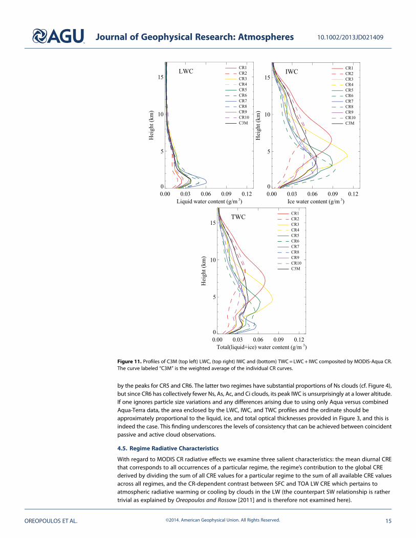
by the peaks for CR5 and CR6. The latter two regimes have substantial proportions of Ns clouds (cf. Figure 4),but since CR6 has collectively fewer Ns, As, Ac, and Ci clouds, its peak IWC is unsurprisingly at a lower altitude.If one ignores particle size variations and any differences arising due to using only Aqua versus combinedAqua-Terra data, the area enclosed by the LWC, IWC, and TWC profiles and the ordinate should beapproximately proportional to the liquid, ice, and total optical thicknesses provided in Figure 3, and this isindeed the case. This finding underscores the levels of consistency that can be achieved between coincidentpassive and active cloud observations.

4.5. Regime Radiative Characteristics

With regard to MODIS CR radiative effects we examine three salient characteristics: the mean diurnal CREthat corresponds to all occurrences of a particular regime, the regime’s contribution to the global CREderived by dividing the sum of all CRE values for a particular regime to the sum of all available CRE valuesacross all regimes, and the CR-dependent contrast between SFC and TOA LW CRE which pertains toatmospheric radiative warming or cooling by clouds in the LW (the counterpart SW relationship is rathertrivial as explained by Oreopoulos and Rossow [2011] and is therefore not examined here).

Figure 11. Profiles of C3M (top left) LWC, (top right) IWC and (bottom) TWC=LWC+ IWC composited by MODIS-Aqua CR.The curve labeled “C3M” is the weighted average of the individual CR curves.



The interpretation of the results that follow is aidedby recalling that the CRE (SW, LW; TOA, or SFC) canbe written as

CRE ¼ Ac Fclr � Fovc f pc; τð Þ½ �ð Þ (1)

where Fclr and Fovc are the cloudless (zero cloudfraction) and overcast (100% cloud fraction) radiativefluxes, Ac is the gridcell total cloud fraction(representing either CFs or CFm for the purposes ofthe discussion here), pc is the mean cloud pressure(top or bottom), τ is the cloud optical thickness, and fis the function that describes their covariabilitywithin the cloudy portion of the gridcell, for example,as a joint probability density function. For fixed Fclr,therefore, CRE depends strongly on cloud fraction,cloud opacity as represented by τ (primarily for SWCRE and secondarily for LW CRE), and cloud verticallocation as represented by pc (primarily for LW CREand to a lesser extent for SW CRE). For fixed cloudconditions, the CRE of course also depends onsurface and atmospheric temperatures (for LW), andTOA solar insolation and surface albedo (for SW). Oneshould also recall that when radiative transfercalculations are involved in estimating or adjustingCRE, as in the CERES SYN1deg product used here,

the cloud optical property values are not the same as those used to derive the regimes [cf. Kato et al., 2011;Minnis et al., 2011]. Without detailed comparisons on how the optical property distributions differ betweenthe two algorithms for each CR, which is beyond the scope of our study, it remains unknown whether thereare any measurable effects on the regime versus CRE mapping presented below.4.5.1. Regime Mean CREWe adopt plots similar to those inOreopoulos and Rossow [2011, hereinafter OR11] to summarize regime CREson a global scale. There is a major difference with the plots of that paper, however: The CREs from CERESbeing used here to calculate the mean values for each regime do not correspond to fluxes at the nominaltime of the regime observation, as in the previous ISCCP analysis, but rather to the diurnal flux averages forthe regime’s gridcell on that particular day. This makes the SW CREs much smaller in the current analysis thanin OR11 since the zero values of the nighttime period are also included in the average.

Figure 12 provides a synopsis of MODIS CR mean global TOA CREs by averaging individual diurnal CREs foreach regime. A result that strikes an immediate impression is that no CR exhibits positive mean net CRE,although two regimes, CR2 and CR10, come close. The strongest mean TOA CRE, for both SW and LW comesfrom CR1, followed in the SW by CR3, which has, however, about the same LW CRE as CR2. These threeregimes have the highest proportion of high clouds, some of which can be substantially thick optically. Agroup of five regimes (CR2 and CR4–7) has similar SW TOA CRE, within ~20Wm�2, but quite a large range ofLW TOA CRE, about ~40Wm�2 (note that the total SW CRE range across regimes is about 100Wm�2, whilethe LW CRE range is about 60Wm�2). Note that all regimes in this group have very similar mean total cloudfractions CFs and CFm (section 3.2), so the LW TOA CRE diversity comes mainly from vertical locationdifferences of the most common cloud types (cf. Figure 1 and equation (1)).

Regimes dominated by low clouds (CR6–9) exhibit low values of LW TOA CRE (~20Wm�2 or below) asexpected. CR10, our most prevalent regime, despite being comprised by substantial amounts of high clouds,belongs clearly to the group of weak LW TOA CREs rather than the group of strong values (consisting of CR1-4and perhaps CR5). Almost certainly, the influence of its high clouds is tempered by its small cloud fraction.Actually, note that the group of regimes closest to the upper left corner of the graph, with the smallest SW andLW TOA CRE effects (CR8–10) comprises the regimes with the smallest cloud fractions, a reminder of the greatinfluence of Ac on CRE magnitude.

Figure 12. Global mean LW and SW CREs for each MODIScloud regime. The dashed lines are isolines of constant netCRE. Also included is information about the spatial variabilityof multiannual mean CRE of each regime which was calcu-lated by taking the standard deviation of all multiannualmean gridcell values, and is shown as horizontal and verticalerror bars whose length is one tenth of the standard devia-tion value. These error bars therefore do not represent theerrors to the displayed means which are minute.



We have also included in this figure informationabout the spatial variability of multiannual mean CREof each regime. This was calculated by taking thespatial standard deviation of all multiyear annualmean gridcell values and is included in the graphas horizontal and vertical error bars that represent1/10th of the actual standard deviation value.These error bars therefore do not represent theerrors to the displayed means which are minute. Ingeneral, greater mean CRE values also correspondto larger standard deviations. Given the largeseasonal and geographical changes of solarinsolation, one would expect the SW TOA CREstandard deviations to be much greater than theirLW counterparts, but it appears that the absence ofa strong hemispherical asymmetry in CR occurrence(on an annual basis at least) dampens the hugesolar insolation variance throughout the year, andtherefore a great potential contributor to variabilityof the SW TOA CRE. The values of spatial standard

deviation are nonetheless large, indicating that the same CR, depending on specific conditions, cangenerate a very wide range of CRE responses at least on daily scales, a finding that mirrors OR11 for ISCCPweather states.4.5.2. Regime Contributions to Global CREThe mean diurnal CREs of individual CRs provide only one aspect of regime radiative importance. Highmean CRE values of a rarely encountered regime may be of small radiative consequence overall, whilethe opposite can also be true, namely, a regime of relatively modest mean CRE may be an importantradiative player if it occurs often. Both scenarios flesh out in the results of Figure 13, which shows thepercentage TOA SW and LW CRE contributions of each regime: CR7 and CR10 are the largest contributors to theSW and LW global TOA CRE, respectively, largely because they rank third and first in RFO and not becausethe global means of their daily values are large. CR9, which has the second largest RFO, is also the secondlargest SW TOA CRE contributor. The remaining CRs huddle together toward the lower left of Figure 13 withcontributions falling within a narrow approximate range of 3–12% for both SW and LW TOA CRE. Within

that group, one can find CRs with widely different globalmean CREs, but almost identical percent contributions:compare for example CR1 and CR8, with equal SW CREcontribution in Figure 13, yet completely different meandiurnal CREs (Figure 12); or, similarly, CR4 and CR8for LW CRE.

Note that because the net CRE can take (and almostalways does) negative values and the global net CREitself is negative, contributions to this quantity can alsobe negative. The strongest negative contributions comefrom CR2 and CR10, the two regimes with near zeroglobal mean net TOA CRE. The physical meaning of thenegative net CRE contribution is that a regime reduces inabsolute terms the value of the negative net CRE, i.e., itpushes it toward positive values.4.5.3. TOA Versus Surface LW CREDepending on their vertical location, and to a lesserdegree, optical properties, clouds either enhance orreduce the overall tendency of the atmosphere toradiatively cool. The weather state concept has proven

Figure 13. Similar to Figure 12 (without the spatial variabil-ity information) but for the percentage contributions ofindividual cloud regimes to the global LW and SW CRE.

Figure 14. SFC (downwelling) versus TOA (upwelling)mean LW CRE of the various MODIS CRs. Horizontaland vertical error bars have the same meaningas in Figure 12.



successful in past work (OR11) in providing a clear separation between warming and cooling inducing weatherstates at thermal infrared wavelengths (all CRs due to absorption by cloud particles exhibit a slight warmingeffect at solar wavelengths, and we therefore do not revisit this trivial result here). As explained in that paper,CRs falling below the diagonal of equal value in a plot of LW SFC CRE versus LW TOA CRE induce radiativewarming and those above the diagonal radiative cooling. Figure 14 shows a plot of this type for the MODIS CRsand the CERES-based mean LW CREs. As stated in section 2.4, radiative transfer calculations are involved inderiving the (downwelling flux) SFC CREs, based on NASA-LARC MODIS cloud property retrievals [Kato et al.,2011]. Three groups of cloud regimes emerge from this analysis: CR1–4, with high proportions of high clouds,constitute the group of regimes inducing atmospheric radiative warming, while CR6–8, and to a smaller degreeCR9, with prevalence of low clouds constitute the group of regimes inducing radiative cooling. CR5 (manymidlevel clouds) and CR10 (mixture of low and high clouds) are close to the line of zero LW CRE divergence(zero LW atmospheric radiative effect). These results are broadly consistent with the ISCCP-based results ofOR11 when comparing the CRs/weather states whose centroid patterns look alike. Once again, we haveincluded spatial variability information in the plot as error bars indicating the standard deviation of the gridcellmultiyear annual means, similar to Figure 12. The TOA LW CRE error bars are the same as in that figure. Thespatial variability of SFC LW CRE is, in general, larger than that of its TOA counterpart for the CRs for which theSFC CRE is larger than the TOA CRE, namely, the low-cloud-dominated CRs to the left of the diagonal.

Figure 15. GPCP-based histograms of CR daily precipitation and corresponding cumulative frequency curves (with scale given in the right ordinate). Each panel alsoshows each CR’s mean precipitation rate, its contribution to the global precipitation, the standard deviation of all available gridcell daily values (“STD”), and its RFO.The statistics include zero values of precipitation not shown in the histograms themselves. The RFOs of this figure are different from those of Figure 1 because of thecompositing assumptions (i.e., the condition that Aqua and Terra CRs be the same for each gridcell).



4.6. Regime Precipitation Characteristics

A straightforward way to appreciate the different characteristicsof precipitation within each regime is to examineprecipitation rate frequency histograms and cumulativefrequencies for each CR. Once again, we assign a GPCPprecipitation rate value only if the Terra and Aqua regimes areidentical for a particular gridcell and day. Although notrepresented in the histograms themselves, zero gridcellprecipitation values are accounted for in the statistical metricsshown in each panel.

The histograms of Figure 15 capture both the temporal (with 1day resolution) and spatial (with 1° resolution) variability ofeach regime’s precipitation. The histograms make immediatelyobvious that CR1 has the widest precipitation histogram of allregimes, with substantial occurrences of values at the highend of precipitation range (>20mm/d) that are virtually neverencountered in other CRs. The next widest histograms arethose by CR3 and CR2. We also plot in Figure 15 cumulativehistogram curves in order to facilitate quick extraction of thefraction of occurrences higher or lower than certain precipitationrates or the precipitation rates of specific cumulative fractionsof occurrence (e.g., the median precipitation rate, as a specialcase). By construction, the steeper the rise of the cumulativehistogram curve, the smaller the fraction of gridcells withhigh daily precipitation rates. There is an abrupt change in thisslope from CR5 to CR6, with the shape of the curve for thelatter regime being very close to that for regimes CR7-9 and toa lesser extent CR10. Based on the cumulative frequency

curves, the CRs can be grouped into four “precipitation regimes”: CR1, CR2 and CR3, CR4, CR5, and CR10,and CR6-9.

Each of the panels of Figure 15 also includes information that summarizes the global apportionment ofGPCP surface precipitation by MODIS CR. Similar to CRE, we are interested in the mean precipitation of eachregime obtained by averaging the daily precipitation values (including zero precipitation) on the day andlocation of a regime’s occurrence, as well as in the contribution of each CR to the global precipitationbudget. As expected, the summary numerical values of Figure 15 indicate a general, albeit imperfect,correspondence with the mean CR cloud optical thicknesses of Figure 3. CR1’s mean surface precipitationrate dwarfs all others, being about double than the second strongest precipitation producer, CR3. Despiteoccurring in only 6% of gridcells, CR1 contributes about 22% to the overall precipitation. Our regimeindexing scheme (which was completely blind to precipitation) results in the first three regimes having alsothe highest precipitation rates and collectively contributing ~47% to the global total precipitation. Individually,the largest contribution (~28%) comes from the most frequent regime, CR10, despite its small mean cloudfraction CFs or CFm, mean precipitation rate, and the fact that it appears frequently to be not precipitating at all.The weakest rainfall, in terms of both mean rate and contribution, is found for CR6-9, with small RFOsand combinations of modest optical thicknesses and cloud fractions.

As with CRE, the seasonal variation of each regime’s global mean precipitation isminiscule: the standard deviationof the 12 multiannual monthly means never exceeds 0.089mm/d. The day-to-day and gridcell-to-gridcellvariation of each regimes’ annual precipitation, as expressed by the standard deviation of all available gridcellvalues (“STD” in Figure 15) can be, on the other hand, quite large. Given their small mean precipitationrates, CR6-10 feature surprisingly large precipitation variability, with a standard deviation 2–3 times greaterthan the mean. The greatest variability is exhibited by CR10, the most frequent and spatially expansive regime,with a fairly wide distribution of cloud fractions and very large zonal variations of precipitation (not shown).The results of Figure 15 indicate that individual regimes can potentially produce a very broad range ofprecipitation rates and also imply that geographic location (i.e., local environmental conditions) is a major

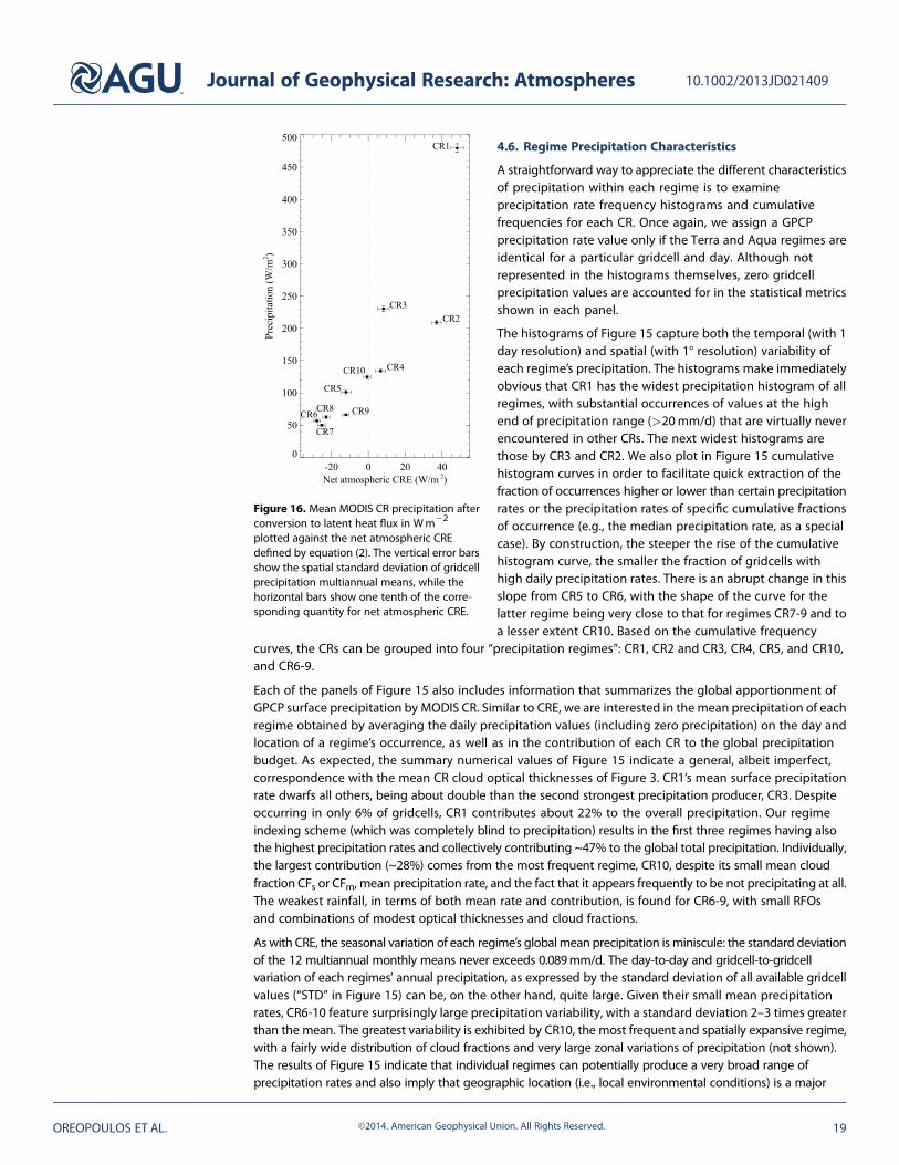
Figure 16. Mean MODIS CR precipitation afterconversion to latent heat flux in Wm�2

plotted against the net atmospheric CREdefined by equation (2). The vertical error barsshow the spatial standard deviation of gridcellprecipitation multiannual means, while thehorizontal bars show one tenth of the corre-sponding quantity for net atmospheric CRE.



contributing factor to the precipitation efficiency of cloud mixtures that appear to share similar height-extinction covariations. This is another way of saying that similarity in these covariations as expressed by thejoint histograms does not translate to trivial within-CR internal variability.

4.7. Radiative Versus Latent Heating by Regime

The energetic imprint on the atmosphere of the combined radiative and precipitative behavior of MODIS CRscan be illuminated by plotting CRmean precipitation converted to energy flux units Wm�2 (mm/dmultipliedby 28.95) [see, for example, Trenberth et al., 2009] against the CRE of the net flux divergence, namely,

CREnetATM ¼ CREnetTOA � CREnetSFC ¼ CRELWTOA þ CRESWTOA� �� CRELWSFC þ CRESWSFC

� �(2)

as shown in Figure 16. Because CRESWTOA≈CRESWSFC;CRE

netATM is positive (indicating radiative heating of the

atmosphere) for the CRs for whichCRELWTOA > CRELWSFC in Figure 14, i.e., those below the diagonal, and vice versa.Figure 16makes immediately apparent that CRs warming the atmosphere radiatively also produce the largestimplicit latent heat warming (CR1–3, and to a lesser extent CR4). On the other hand, the CRs that cool theatmosphere radiatively, CR6-9, also produce weak implicit latent heat warming. Apparently, cloud mixturedecomposition by MODIS CR is successful in revealing clearly that clouds organize at global scales in such away as to induce energy flow tendencies from areas where CRs dominated by high and midlevel clouds ofhigher precipitation rates are more prominent to areas where CRs dominated by low clouds of lowerprecipitation rates prevail. Furthermore, there is evidence that perturbations (anomalies) in individual CRradiative atmospheric warming or cooling are balanced by perturbations in their own latent heat release(via changes in precipitation) as described by Lebsock et al. [2010] who quantified such effects for their ownoceanic tropical MODIS CRs.

5. Summary and Concluding Thoughts

An important step toward in-depth understanding of the role of clouds on the water and energy budget is ameaningful classification of the various cloudmixtures encountered in different parts of the globe at differenttimes of the year. Cloud observations exist from many space-based observational platforms with a variety ofremote sensing algorithms applied to both passive and active sensors. Passive observations have beenavailable longer and have generally much better spatial coverage. In this, as well as in previous work, thisclass of observations was chosen for classifying and grouping mesoscale (i.e., ~1°) cloud mixtures into“weather states” or (as in this paper) “cloud regimes.” Our cloud regime classification yielded 10 regimes forthe globe as a whole and relied on a clustering algorithm applied to cloud optical thickness and cloud toppressure retrievals from measurements of the MODIS radiometer aboard the Terra and Aqua satellites. Amultitude of other data sets was employed to investigate the nature of these cloud regimes beyond what canbe gleaned from the passive observations alone. The essence of the analysis technique was to compositethese complementary data sets as a function of MODIS cloud regime.

The two fundamental objectives of this work were as follows: (a) to examine aspects of the regimes’ nature,including their morphological features and radiative and hydrological importance, as inferred from othercoincident measurements; and (b) to identify the atmospheric conditions that tend to be associated withthe regimes.

Our findings clearly indicate that the regimes obtained from joint histograms of cloud optical thickness andcloud top pressure have very disparate bulk cloud properties and vertical structure. They were distinctlyseparate in terms of dominant water phase (as measured by liquid/ice ratios in both cloud fractions andoptical thickness), mean vertical location of their highest tops and lowest bases, vertical distribution of cloudfraction and water content, and number of overlapping cloud layers. When associated with traditional cloudtype classifications made possible by active observations, their makeup also turned out to be very diverseand consistent with expectations based on interpretation of the passive observations, namely, the “mean”joint histogram representing each regime and the geographical distribution of their occurrences.

The MODIS cloud regimes were also found to form in environments characterized by distinct mesoscalevertical motions and temperature/relative humidity profiles. The regimes that tend to form in regions ofascent were also accompanied by warmer and more humid than average conditions in the lower andmiddle troposphere; these regimes were very often close to overcast and had a large proportion of high



clouds. On the other hand, the regimes forming in regions of weaker dynamical forcing (weaker ascent oreven descent on average) were dominated by low clouds, were less likely to be overcast, and wereassociated with drier and cooler than average low to midtroposphere conditions.

We also applied our straightforward compositing approach on Clouds and the Earth’s Radiant Energy System(CERES) and Global Precipitation Climatology Project (GPCP) daily data of the same 1° spatial resolution as thatof the MODIS regimes for gridcells with identical Terra and Aqua regimes. The analysis revealed the CRs’ distinctradiative and hydrological signatures. For example, even if some CRs had almost identical multiyear annualglobal means of one CRE component (SW or LW), they exhibited diverse values for the other component.Moreover, their contribution to the total global CRE was quite disparate because of strong dependencies onregime frequency of occurrence. CR distinctiveness according to this criterion (resemblance of mean values nottranslating to similarity in contributions) carried to precipitation as well.

No CR exhibited positive net global TOA CRE, although two (comprising different cloud types) had near-zerovalues. This is broadly consistent with previous analysis [Hartmann et al., 1992; Chen et al., 2000; Oreopoulosand Rossow, 2011] and the long-known fact that clouds tend to radiatively cool the planet. A comparisonbetween surface and TOA LW CRE revealed a group of regimes with an atmospheric radiative warming bent(made of regimes with large proportions of high clouds), another group with a cooling predisposition(regimes with many low clouds), and two regimes with a near-neutral effect.

The three CRs that were the strongest precipitation producers, were found to be overall responsible for abouthalf the total global precipitation as recorded by GPCP. These three CRs happened to also have the smallestassigned indices in our empirical regime ordering system which emphasized large total cloud fractions andstrong cloud presence above the middle troposphere. We also showed that the histograms of precipitationvaried greatly by CR and demonstrated unambiguously that the regimes with small precipitation means hadvery abrupt tails on the high end, indicative of a virtual absence of strong precipitation events (according toGPCP at least). Compared to the study of Lee et al. [2013] which, however, was restricted to the tropics only, wedid not see as extreme a separation between precipitation-rich and precipitation-poor cloud regimes.

The concept of cloud regimes with the meaning assigned in the current work is now about 10 years old(it was first introduced by Jakob and Tselioudis [2003]). The ever-growing body of work built around itdemonstrates its acceptance as a promising approach for making sense of a wide range of processesaffecting and being affected by clouds. The present study serves as one more affirmation that cloud regimesderived from cluster analysis of passive satellite retrievals at O (100 km) are an appropriate foundation fordecomposing the Earth’s water and energy budget in a meaningful way. We advocate that this decompositionbe replicated, with the aid of satellite simulators, to the best extent possible in GCMs as a means of identifyingdeficiencies and ultimately improving cloud representations.

ReferencesAckerman, S. A., K. I. Strabala, W. P. Menzel, R. A. Frey, C. Moeller, and L. E. Gumley (1998), Discriminating clear sky from clouds with MODIS,

J. Geophys. Res., 103(D24), 32,141–32,157, doi:10.1029/1998JD200032.Adler, R., C. Kidd, G. Petty, M. Morissey, and H. Goodman (2001), Intercomparison of global precipitation products: The third Precipitation

Intercomparison Project (PIP-3), Bull. Am. Meteorol. Soc., 82, 1377–1396, doi:10.1175/1520-0477(2001)082<1377:IOGPPT>2.3.CO;2.Adler, R., et al. (2003), The version-2 global precipitation climatology project (GPCP) monthly precipitation analysis (1979–present),

J. Hydrometeorol., 4, 1147–1167, doi:10.1175/1525-7541(2003)004<1147:TVGPCP>2.0.CO;2.Anderberg, M. R. (1973), Cluster Analysis for Applications, 359 pp., Elsevier, New York.Chen, T., Y. Zhang, andW. Rossow (2000), Sensitivity of atmospheric radiative heating rate profiles to variations of cloud layer overlap, J. Clim.,

13, 2941–2959, doi:10.1175/1520-0442(2000)013<2941:SOARHR>2.0.CO;2.Gordon, N., and J. Norris (2010), Cluster analysis of midlatitude oceanic cloud regimes: Mean properties and temperature sensitivity, Atmos.

Chem. Phys., 10, 6435–6459, doi:10.5194/acp-10-6435-2010.Gryspeerdt, E., and P. Stier (2012), Regime-based analysis of aerosol-cloud interactions, Geophys. Res. Lett., 39, L21802, doi:10.1029/2012GL053221.Gryspeerdt, E., P. Stier, and D. G. Partridge (2014), Satellite observations of cloud regime development: The role of aerosol processes, Atmos.

Chem. Phys., 14, 1141–1158, doi:10.5194/acp-14-1141-2014.Hartmann, D. L., M. E. Ockert-Bell, and M. L. Michelsen (1992), The effect of cloud type on Earth’s energy balance: Global analysis, J. Clim., 5,

1281–1304, doi:10.1175/1520-0442(1992)005<1281:TEOCTO>2.0.CO;2.Haynes, J., C. Jakob, W. Rossow, G. Tselioudis, and J. Brown (2011), Major characteristics of Southern Ocean cloud regimes and their effects on

the energy budget, J. Clim., 24, 5061–5080, doi:10.1175/2011JCLI4052.1.Jakob, C., and C. Schumacher (2008), Precipitation and latent heating characteristics of the major tropical western Pacific cloud regimes,

J. Clim., 21, 4348–4364, doi:10.1175/2008JCLI2122.1.Jakob, C., and G. Tselioudis (2003), Objective identification of cloud regimes in the tropical western Pacific, Geophys. Res. Lett., 30(21), 2082,

doi:10.1029/2003GL018367.



AcknowledgmentsFunding from NASA’s Modeling Analysisand Prediction, CloudSat/CALIPSO, andthe Science of Terra and Aqua programsis gratefully acknowledged. We wouldlike to thank Robert Pincus and StevenPlatnick for helpful discussions on ISCCPand MODIS cloud property retrievaldifferences and the reviewers forconstructive suggestions that helped usgreatly to improve the paper. Pleasecontact the lead author for freelyobtaining the MODIS cloud regime dataused in this paper.

Jakob, C., G. Tselioudis, and T. Hume (2005), The radiative, cloud, and thermodynamic properties of the major tropical western Pacific cloudregimes, J. Clim., 18, 1203–1215, doi:10.1175/JCLI3326.1.

Kato, S., S. Sun-Mack, W. F. Miller, F. G. Rose, Y. Chen, P. Minnis, and B. A. Wielicki (2010), Relationships among cloud occurrence frequency,overlap, and effective thickness derived from CALIPSO and CloudSat merged cloud vertical profiles, J. Geophys. Res., 115, D00H28,doi:10.1029/2009JD012277.

Kato, S., et al. (2011), Improvements of top-of-atmosphere and surface irradiance computations with CALIPSO, CloudSat, and MODIS derivedcloud and aerosol properties, J. Geophys. Res., 116, D19209, doi:10.1029/2011JD16050.

Lebsock, M., C. Kummerow, and G. Stephens (2010), An observed tropical oceanic radiative-convective cloud feedback, J. Clim., 23,2065–2078, doi:10.1175/2009JCLI3091.1.

Lee, D., L. Oreopoulos, G. Huffman, W. Rossow, and I. Kang (2013), The precipitation characteristics of ISCCP tropical weather states, J. Clim.,26, 772–788, doi:10.1175/JCLI-D-11-00718.1.

Marchand, R., T. Ackerman, M. Smyth, and W. B. Rossow (2010), A review of cloud top height and optical depth histograms from MISR, ISCCP,and MODIS, J. Geophys. Res., 115, D16206, doi:10.1029/2009JD013422.

Minnis, P., W. L. Smith, Jr., D. P. Garber, J. K. Ayers, D. R. Doelling (1994), Cloud properties derived from GOES-7 for Spring 1994 ARM IntensiveObserving Period using version 1.0.0 of ARM satellite data analysis program, NASA Reference Publication 1366.

Minnis, P., et al. (2011), CERES Edition-2 cloud property retrievals using TRMM VIRS and Terra and Aqua MODIS data, Part I: Algorithms, IEEETrans. Geosci. Remote Sens., 49, 4374–4400, doi:10.1109/TGRS.2011.2144601.

Oreopoulos, L., and W. Rossow (2011), The cloud radiative effects of International Satellite Cloud Climatology Project weather states,J. Geophys. Res., 116, D12202, doi:10.1029/2010JD015472.

Pincus, R., S. Platnick, S. Ackerman, R. Hemler, and R. Hofmann (2012), Reconciling simulated and observed views of clouds: MODIS, ISCCP,and the limits of instrument simulators, J. Clim., 25, 4699–4720, doi:10.1175/JCLI-D-11-00267.1.

Rienecker, M., et al. (2011), MERRA: NASA’s Modern-Era Retrospective Analysis for research and applications, J. Clim., 24, 3624–3648,doi:10.1175/JCLI-D-11-00015.1.

Rossow, W., G. Tselioudis, A. Polak, and C. Jakob (2005), Tropical climate described as a distribution of weather states indicated by distinctmesoscale cloud property mixtures, Geophys. Res. Lett., 32, L21812, doi:10.1029/2005GL024584.

Rossow, W., A. Mekonnen, C. Pearl, and W. Goncalves (2013), Tropical precipitation extremes, J. Clim., 26, 1457–1466, doi:10.1175/JCLI-D-11-00725.1.

Sassen, K., and Z. Wang (2008), Classifying clouds around the globe with the CloudSat radar: 1-year of results, Geophys. Res. Lett., 35, L04805,doi:10.1029/2007GL032591.

Tan, J., and C. Jakob (2013), A three-hourly data set of the state of tropical convection based on cloud regimes, Geophys. Res. Lett., 40, 1415–1419,doi:10.1002/grl.50294.

Tian, B., E. Fetzer, B. Kahn, J. Teixeira, E. Manning, and T. Hearty (2013), Evaluating CMIP5 models using AIRS tropospheric air temperature andspecific humidity climatology, J. Geophys. Res. Atmos., 118, 114–134, doi:10.1029/2012JD018607.

Trenberth, K. E., J. T. Fasullo, and J. Kiehl (2009), Earth’s global energy budget, Bull. Am. Meteorol. Soc., 90, 311–323, doi:10.1175/2008BAMS2634.1.Tselioudis, G., W. Rossow, Y. Zhang, and D. Konsta (2013), Global weather states and their properties from passive and active satellite cloud

retrievals, J. Clim., 26, 7734–7746, doi:10.1175/JCLI-D-13-00024.1.Williams, K., and G. Tselioudis (2007), GCM intercomparison of global cloud regimes: Present-day evaluation and climate change response,

Clim. Dyn., 29, 231–250, doi:10.1007/s00382-007-0232-2.Williams, K., and M. Webb (2009), A quantitative performance assessment of cloud regimes in climate models, Clim. Dyn., 33, 141–157,

doi:10.1007/s00382-008-0443-1.Yin, X., A. Gruber, and P. Arkin (2004), Comparison of the GPCP and CMAP merged gauge-satellite monthly precipitation products for the

period 1979–2001, J. Hydrometeorol., 5, 1207–1222, doi:10.1175/JHM-392.1.Zhang, Y., S. Klein, G. Mace, and J. Boyle (2007), Cluster analysis of tropical clouds using CloudSat data, Geophys. Res. Lett., 34, L12813,

doi:10.1029/2007GL029336.



an examination of the nature of global modis cloud regimes · an examination of the nature of...

Documents