an ex post economic analysis impact of hybrix 5 sweet...

Contributed paper for the 53rd Annual Conference of the Australian Agricultural and Resource Economics Society at Sebel Cairns Hotel, Cairns, 11-13 February 2009

An Ex-Post Economic Analysis of the Hybrix5 Sweet Corn Breeding Program in Queensland

By Mary Ann Franco-Dixon, DVM, PGAgEconStud, MAgEcon, PhD Queensland Department of Primary Industries, GPO Box 46, Brisbane Q 4001

ph 07 3239 6787 fax 07 3221 4049 email [email protected] Abstract The $2.1 million invested for the sweet corn research breeding program resulted in the release of Hybrix5 in 1995 which is a new sweet corn variety with improved insect and disease resistance. Based on the ex-post evaluation of this research program, it was estimated that the net benefits of the program up to 2006 (in 2006 dollars) is around $3 million. The producer benefits are 4.5 times the costs of R&D. Extending the period up to 2012 (20 years) resulted in estimated net benefits of around $6 million in 2006 dollars. The producer benefits are 7.2 times the costs of the R&D. Key words: Hybrid5, Sweet corn, Ex-post evaluation Disclaimer The author is responsible for any errors. Opinions expressed are of the author and do not necessarily represent the policy of the Queensland Department of Primary Industries and Fisheries. Acknowledgement The contributions, in regards to the economic analysis, of Fred Chudleigh, Trevor Wilson, George Antony and Thom Goodwin in this analysis are gratefully acknowledged. The inputs of Ian Martin and Rodney Emerick regarding the Hybrix5 research results and industry data are also acknowledged.

Contributed paper- 53rd AARES Conference February 2009 1

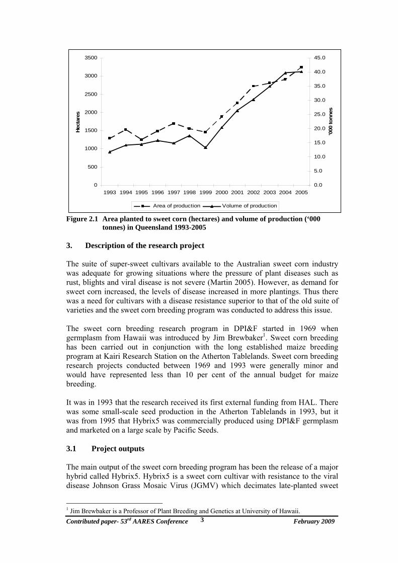
1. Introduction The sweet corn industry in Australia has grown significantly in terms of volume and value of production for the last 13 years (1993-2005). The increase in sweet corn production for the last 13 years in Queensland could be partly attributed to the introduction and adoption of a hybrid variety called Hybrix5. The use of Hybrix5 increases the sweet corn yield due to resistance to disease and lengthening of the planting window. Queensland produced 41 per cent of the total national sweet corn production in 2005. The Department of Primary Industries and Fisheries (DPI&F) and the then Horticulture Research Development Corporation, HRDC (now Horticulture Australia Limited - HAL), invested money in sweet corn breeding research that developed Hybrix5. Although experimental and observed data have shown that this seed variety has been an improvement on the pre-Hybrix5 varieties, there was no study to demonstrate the significant payoffs from the investment on this research. The aim of this paper is thus to provide the results of an assessment of the economic benefits of the Hybrix5 research breeding program. 2. Sweet corn industry The Australian sweet corn industry is estimated to have had an annual farm gate value in excess of $70 million in 2005 (Martin 2005). Sweet corn per-capita consumption in Australia increased from 3.5 kg in 1997 to 6 kg in 2001. Improved presentation in supermarkets through the use of pre-packs rather than loose cobs has helped to establish sweet corn as a popular item in households’ shopping lists. As shown in Figure 2.1, the volume of sweet corn production in Queensland increased by 241 per cent from around 11 800 tonnes in 1993 to 40 200 tonnes in 2005. This has been achieved by widening the planting window and by expanding the area under production. Figure 2.1 shows that area planted to sweet corn increased by 150 per cent from only around 1 300 hectares in 1993 to 3 250 hectares in 2005. In the Lockyer Valley, the planting window has been increased significantly by the introduction of Hybrix5, a hybrid with resistance to Johnson Grass Mosaic Virus. Sweet corn can now be planted from September to March, about three months later than the usual practice for varieties prior to Hybrix5. This development means that the number of successive plantings has substantially increased. At Bowen in north Queensland, there has been a large expansion in the area planted to sweet corn, with the likelihood of more plantings.


0

500

1000

1500

2000

2500

3000

3500

1993 1994 1995 1996 1997 1998 1999 2000 2001 2002 2003 2004 2005

Hect

ares

0.0

5.0

10.0

15.0

20.0

25.0

30.0

35.0

40.0

45.0

'000

tonn

es

Area of production Volume of production

Figure 2.1 Area planted to sweet corn (hectares) and volume of production (‘000 tonnes) in Queensland 1993-2005

3. Description of the research project The suite of super-sweet cultivars available to the Australian sweet corn industry was adequate for growing situations where the pressure of plant diseases such as rust, blights and viral disease is not severe (Martin 2005). However, as demand for sweet corn increased, the levels of disease increased in more plantings. Thus there was a need for cultivars with a disease resistance superior to that of the old suite of varieties and the sweet corn breeding program was conducted to address this issue. The sweet corn breeding research program in DPI&F started in 1969 when germplasm from Hawaii was introduced by Jim Brewbaker1. Sweet corn breeding has been carried out in conjunction with the long established maize breeding program at Kairi Research Station on the Atherton Tablelands. Sweet corn breeding research projects conducted between 1969 and 1993 were generally minor and would have represented less than 10 per cent of the annual budget for maize breeding. It was in 1993 that the research received its first external funding from HAL. There was some small-scale seed production in the Atherton Tablelands in 1993, but it was from 1995 that Hybrix5 was commercially produced using DPI&F germplasm and marketed on a large scale by Pacific Seeds. 3.1 Project outputs The main output of the sweet corn breeding program has been the release of a major hybrid called Hybrix5. Hybrix5 is a sweet corn cultivar with resistance to the viral disease Johnson Grass Mosaic Virus (JGMV) which decimates late-planted sweet


1 Jim Brewbaker is a Professor of Plant Breeding and Genetics at University of Hawaii.

corn crops especially in the Lockyer Valley. Crops planted for harvest from January to April are particularly prone to infection. Hybrix5 also has good resistance to common rust (Puccinia sorghi) and to the major insect pest of sweet corn, Heliothis corn ear worm. Thus, there is less need for fungicides such as chorothalonil and insecticides such as Lannate resulting in significant reduction in growing costs. 3.2 Project outcomes2 • Adoption of Hybrix5 among sweet corn growers with greater confidence

about a successful crop outcome; • Longer growing season with planting extended from the conventional 4

months (September to December) to approximately 6 to 7 months into January, February or March. This translates into an increase in sweet corn production and longer availability of fresh sweet corn with a consequent reduction in the scale and cost of warehousing;

• Improved sweet corn yield; • Higher kernel recovery percentage that reduces post-harvest transportation

costs by reducing the number of corn truckloads for a given output of kernels; • Reduction in the number and cost of insecticide sprays for Heliothis and

fungicide sprays for the common rust; and • Export of seed stock from new sweet corn cultivars to other sweet corn

producing countries. 4. Methodology An ex-post cost benefit analysis (CBA) was conducted to evaluate and compare the benefits flowing from the sweet corn breeding program. The benefit of the sweet corn breeding program is evaluated by comparing the state of the market and industry “with the innovation” to a forecast of their state “without the innovation”. Benefits and costs are compared over time, using a discount rate. The two criteria used in the CBA were the Net Present Value (NPV) and Benefit Cost Ratio (BCR). 5. Project costs In current value terms, the total cost to DPI&F of the Hybrix5 breeding research over 1969 to 2005 was $1.98 million. HRDC contributed an additional $111 555 in 1994 and 1995, increasing the total research cost to $2.092 million. 5.1 Costs of Hybrix 5 sweet corn breeding activities The Hybrix5 sweet corn breeding program started in 1969 as a minor project that needed only 0.1 full-time equivalent (FTE) personnel until 1983. Allocation increased to 0.3 FTE from 1983 to 1993 and then significantly increased to 3.48


2 Martin 2006, pers. comm.

FTEs prior to the release of Hybrix5 for the years 1994 and 1995. Wages and salary costs (including an allowance for on-costs) were about $28 thousand per annum. No domestic or overseas travel cost was charged to the project but total operating expenses added annually another $11 thousand on average. This results in a total average direct cost of $39 thousand (Table 5.1). The costs of the provision of facilities and services for sweet corn breeding and associated activities are incorporated into costs as ‘corporate overheads’ allowance calculated at 1.77 times the initial salaries and wages paid. By including the corporate on-costs, $39 thousand per annum was added to the costs of carrying out sweet corn breeding program.

Table 5.1 Project costs (2006 dollars)

Year Labour Costs

Operating Costs

Total Capital Costs

Total Direct Project Costs

Corporate Overheads Allowance

Total Project Costs

$’000 $’000 $’000 $’000 $’000 $’000 1969 10 2 0 12 14 26 1970 10 2 0 12 14 26 1971 10 2 0 12 14 26 1972 10 2 0 12 14 26 1973 10 2 0 12 14 26 1974 10 2 0 12 14 26 1975 10 2 0 12 14 26 1976 10 2 0 12 14 26 1977 10 2 0 12 14 26 1978 10 2 0 12 14 26 1979 10 2 0 12 14 26 1980 10 2 0 12 14 26 1981 10 2 0 12 14 26 1982 10 2 0 12 14 26 1983 10 2 0 12 14 26 1984 30 7 0 37 42 79 1985 30 7 0 37 42 79 1986 30 7 0 37 42 79 1987 30 7 0 37 42 79 1988 30 7 0 37 42 79 1989 30 7 0 37 42 79 1990 30 7 0 37 42 79 1991 30 7 0 37 42 79 1992 30 7 0 37 42 79 1993 30 7 0 37 42 79 1994 151 42 0 194 211 405 1995 151 145 0 296 211 507 Total 748 299 0 1 047 1 045 2 092

5.2 Source of funds External funds from the then HRDC (now HAL) started in 1993 and, as shown in Table 5.2, provided only 1 per cent of the total 1994 fund budget of $400 thousand. This external HRDC funding, however, received a considerable boost from around $5 thousand in 1993 to 1994 to around $107 thousand in 1994 to 1995 which is a 21 per cent share of the total funding for the sweet corn breeding program. Of the total


costs of $2.1 million, DPI&F has provided 95 per cent of the cost of the project and HRDC provided 5 per cent. Table 5.2 Fund sources (2006 dollars)

Year DPI&F HRDC Total $’000 $’000 $’000

1969 to 1983 26 annually 0 26 annually 1984 to 1993 79 annually 0 79 annually

1994 400 5 405 1995 400 107 507 Total 1 980 112 2 092

% of Total 95% 5% 100% 6. Estimation of Project Benefits For this study, the approximate measures of benefit from the innovation adoption (which in this case is the use of Hybrix5 seed) used were: • The increase in the level of output produced by adopters of the Hybrix5 seeds;

and • The reduction of average cost of production due to less chemical costs

attributable to the adoption of Hyrbrix5. 6.1 ‘Without Hybrix5 research’ scenario In the ‘without Hybrix5 scenario”, it was assumed that sweet corn yield and thus production would have remained static (Rodney Emerick, pers. comm. 2007). Also, the area planted to sweet corn was not expected to change. Consequently, production costs remained the same. 6.2 ‘With Hybrix5 research’ scenario In the ‘with Hybrix5 research’ scenario, it was assumed that there is a crop yield increase of 20 per cent and an annual 5 per cent increase in area planted to Hybrix5 (Rodney Emerick, pers. comm. 2007). This is because Hybrix5 is resistant to Johnson Grass Mosaic Virus which allows for a year round production of sweet corn ensuring a 12-month supply. It is also assumed that the increase in demand for sweet corn is met mainly by the increase in production due to increase in yield. 6.3 Economic surplus method This section is heavily based on Masters et al. (1996). To analyse the value of the Hybrix5 breeding programs, the economic surplus in a situation “with this research” was compared to an alternative situation “without this research” which were both described above. In the economic surplus method, agronomic data are turned into economic values by using the concept of supply-demand equilibrium (Masters et al. 1996). ‘Supply’ represents producers’ production costs and profits and ‘demand’ represents consumers’ consumption values. Some ‘equilibrium’ quantity and price result from the interaction of these two forces. Economic welfare depends not only on the equilibrium price and quantity which may be directly observed in the market, Contributed paper- 53rd AARES Conference February 2009 6

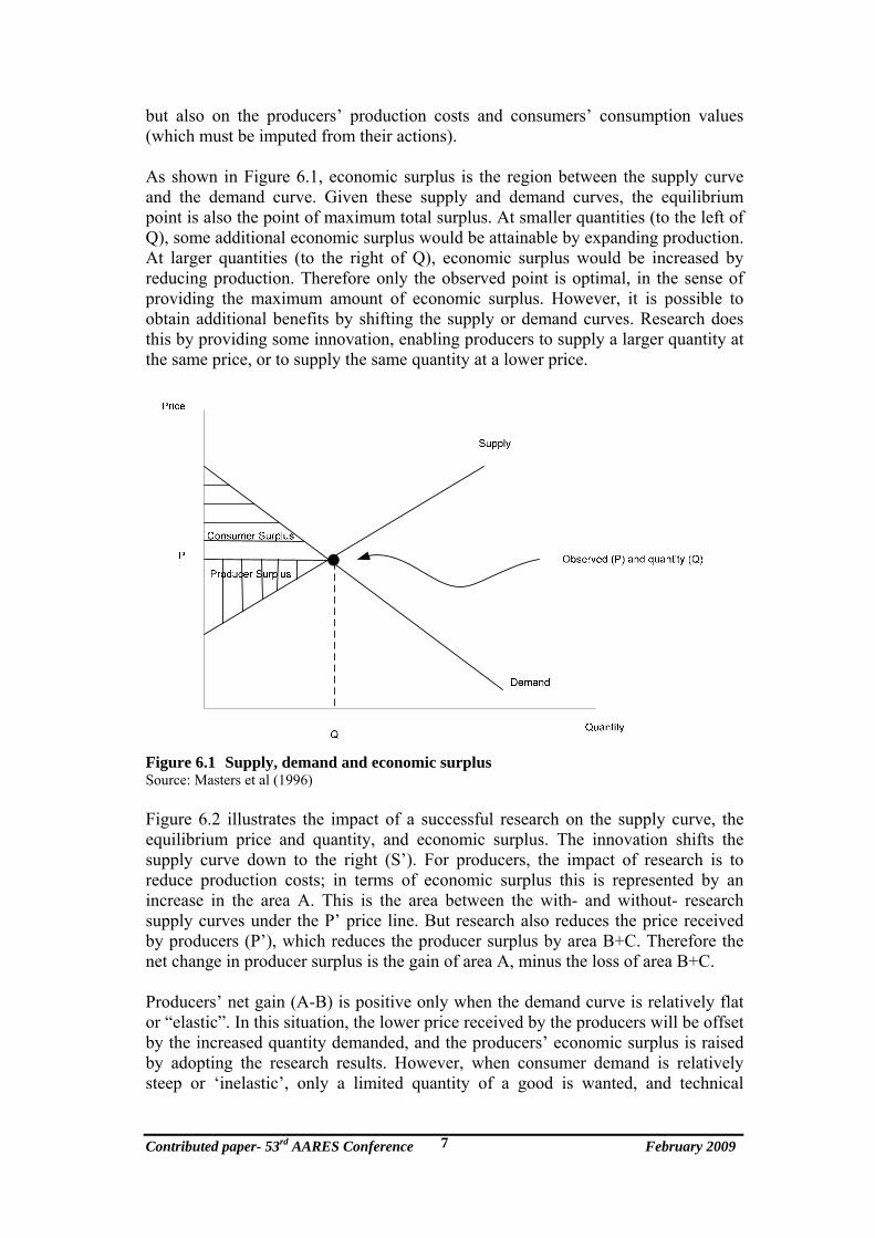
but also on the producers’ production costs and consumers’ consumption values (which must be imputed from their actions). As shown in Figure 6.1, economic surplus is the region between the supply curve and the demand curve. Given these supply and demand curves, the equilibrium point is also the point of maximum total surplus. At smaller quantities (to the left of Q), some additional economic surplus would be attainable by expanding production. At larger quantities (to the right of Q), economic surplus would be increased by reducing production. Therefore only the observed point is optimal, in the sense of providing the maximum amount of economic surplus. However, it is possible to obtain additional benefits by shifting the supply or demand curves. Research does this by providing some innovation, enabling producers to supply a larger quantity at the same price, or to supply the same quantity at a lower price.

Figure 6.1 Supply, demand and economic surplus Source: Masters et al (1996) Figure 6.2 illustrates the impact of a successful research on the supply curve, the equilibrium price and quantity, and economic surplus. The innovation shifts the supply curve down to the right (S’). For producers, the impact of research is to reduce production costs; in terms of economic surplus this is represented by an increase in the area A. This is the area between the with- and without- research supply curves under the P’ price line. But research also reduces the price received by producers (P’), which reduces the producer surplus by area B+C. Therefore the net change in producer surplus is the gain of area A, minus the loss of area B+C. Producers’ net gain (A-B) is positive only when the demand curve is relatively flat or “elastic”. In this situation, the lower price received by the producers will be offset by the increased quantity demanded, and the producers’ economic surplus is raised by adopting the research results. However, when consumer demand is relatively steep or ‘inelastic’, only a limited quantity of a good is wanted, and technical


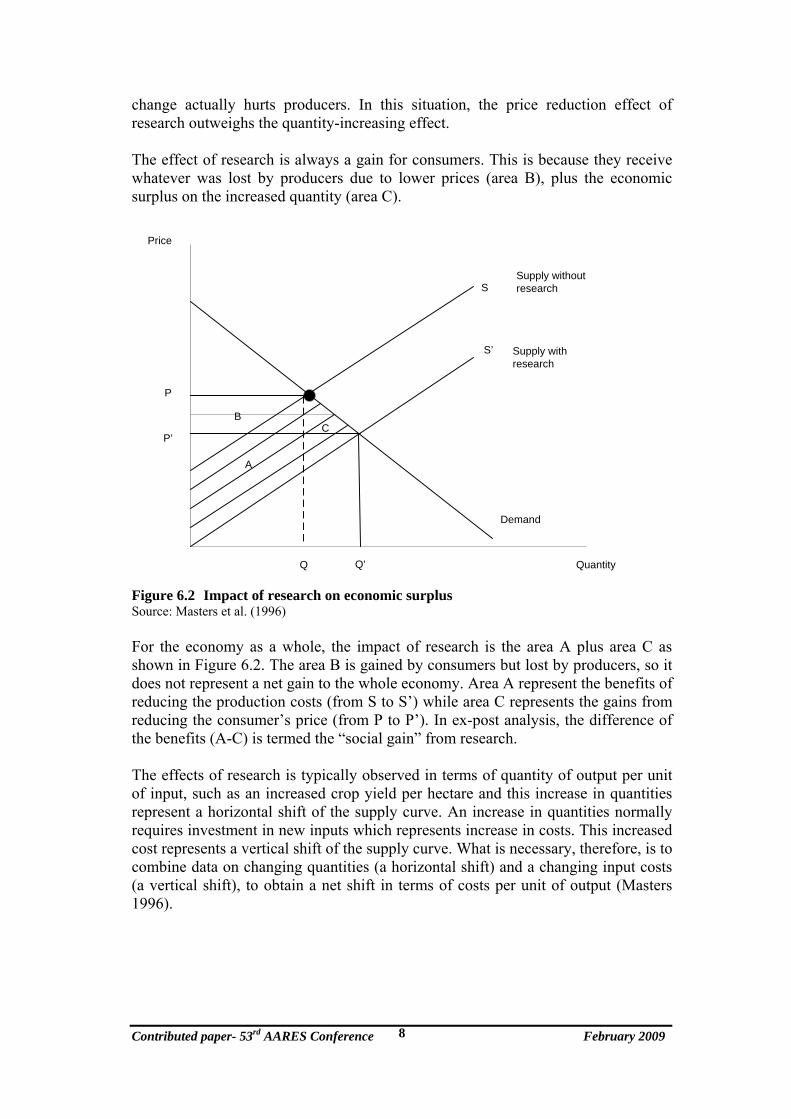
change actually hurts producers. In this situation, the price reduction effect of research outweighs the quantity-increasing effect. The effect of research is always a gain for consumers. This is because they receive whatever was lost by producers due to lower prices (area B), plus the economic surplus on the increased quantity (area C).

Demand

Supply without research

Q

P

Quantity

Price

P’

Q’

C

A

B

Supply with research

S

S’

Figure 6.2 Impact of research on economic surplus Source: Masters et al. (1996) For the economy as a whole, the impact of research is the area A plus area C as shown in Figure 6.2. The area B is gained by consumers but lost by producers, so it does not represent a net gain to the whole economy. Area A represent the benefits of reducing the production costs (from S to S’) while area C represents the gains from reducing the consumer’s price (from P to P’). In ex-post analysis, the difference of the benefits (A-C) is termed the “social gain” from research. The effects of research is typically observed in terms of quantity of output per unit of input, such as an increased crop yield per hectare and this increase in quantities represent a horizontal shift of the supply curve. An increase in quantities normally requires investment in new inputs which represents increase in costs. This increased cost represents a vertical shift of the supply curve. What is necessary, therefore, is to combine data on changing quantities (a horizontal shift) and a changing input costs (a vertical shift), to obtain a net shift in terms of costs per unit of output (Masters 1996).


6.4 Application of the economic surplus method to the Hybrix5 breeding research

Figure 6.3 illustrates how to estimate both the horizontal and vertical shifts and how to combine the data in a typical impact assessment.

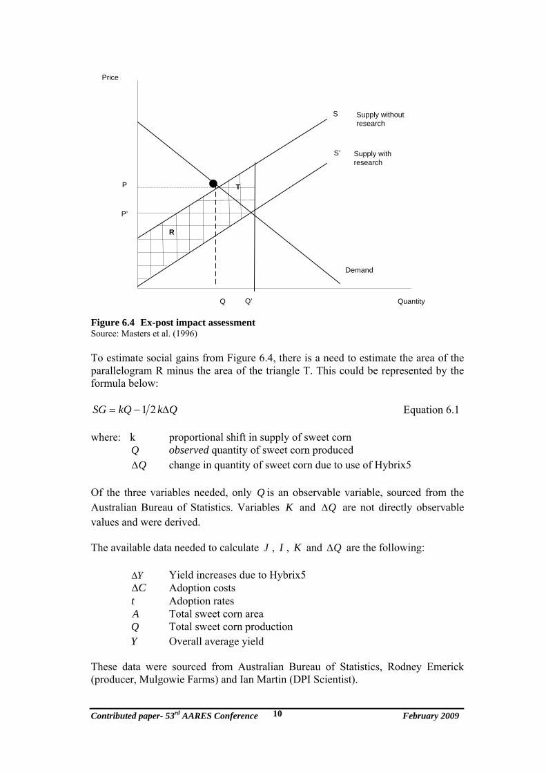
Figure 6.3 Estimating supply shifts using observed data Source: Masters et al. (1996) In the Hybrix5 breeding research, sweet corn output increases for a given set of inputs, by the quantity J, from supply curve S to S”. The relevant observed data available is in terms of yield per hectare (e.g. kg/ha). To calculate J or production shift (see Figure 6.3), the increase in yield (kg/ha) due to Hybrix5 is multiplied by adoption rate (the proportion of Hybrix5 area) and then by total sweet corn area (ha). As Figure 6.4 shows, ex-post impact assessments using the economic surplus approach are based on estimating the magnitude of cost reductions given the observed level of output (i.e., area R) and then making an adjustment for the change in quantity associated with a change in price (i.e., area T).


Demand

Supply without research

Q

P

Quantity

Price

P’

Q’

T

R

Supply with research

S

S’

Figure 6.4 Ex-post impact assessment Source: Masters et al. (1996) To estimate social gains from Figure 6.4, there is a need to estimate the area of the parallelogram R minus the area of the triangle T. This could be represented by the formula below:

QkkQSG ∆−= 21 Equation 6.1 where: k proportional shift in supply of sweet corn observed quantity of sweet corn produced Q change in quantity of sweet corn due to use of Hybrix5 Q∆ Of the three variables needed, only Q is an observable variable, sourced from the Australian Bureau of Statistics. Variables K and Q∆ are not directly observable values and were derived. The available data needed to calculate J , I , K and Q∆ are the following:

Y∆ Yield increases due to Hybrix5 C∆ Adoption costs

Adoption rates t A Total sweet corn area Total sweet corn production Q Y Overall average yield These data were sourced from Australian Bureau of Statistics, Rodney Emerick (producer, Mulgowie Farms) and Ian Martin (DPI Scientist).


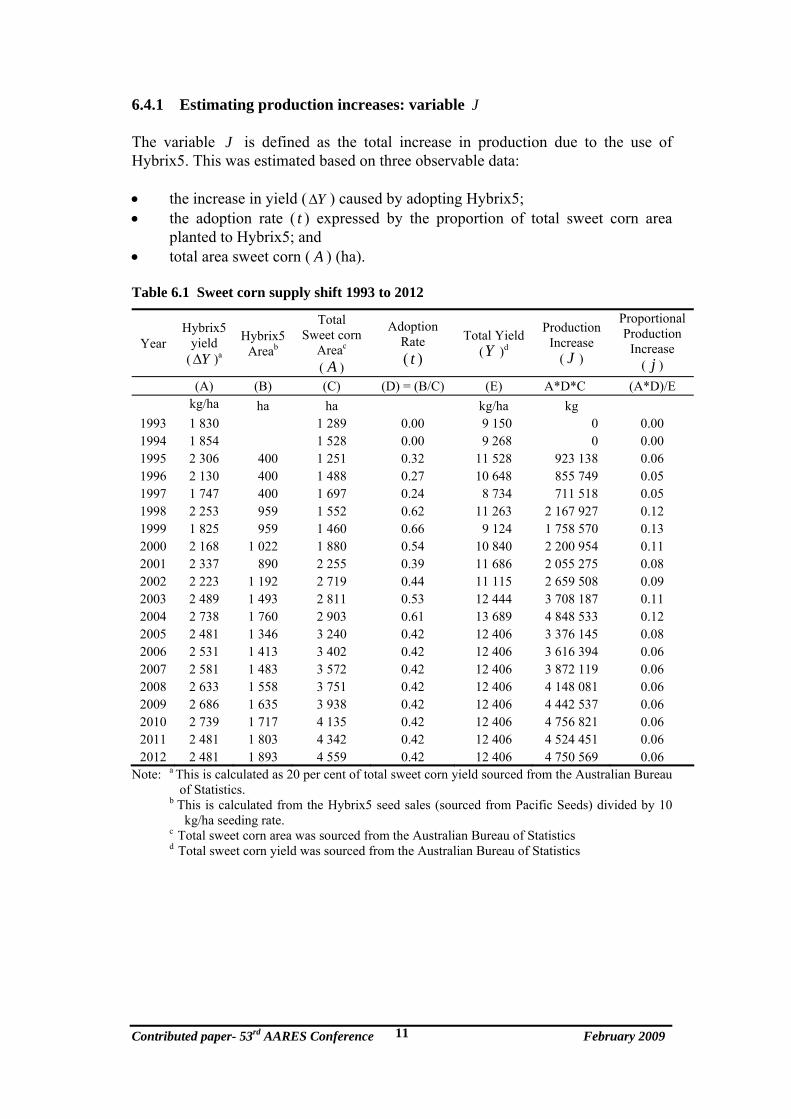
6.4.1 Estimating production increases: variable J The variable J is defined as the total increase in production due to the use of Hybrix5. This was estimated based on three observable data: • the increase in yield ( ) caused by adopting Hybrix5; Y∆• the adoption rate ( t ) expressed by the proportion of total sweet corn area

planted to Hybrix5; and • total area sweet corn ( A ) (ha). Table 6.1 Sweet corn supply shift 1993 to 2012

Year Hybrix5

yield ( )Y∆ a

Hybrix5 Areab

Total Sweet corn

Areac

( A )

Adoption Rate ( t )

Total Yield (Y )d

Production Increase

( J )

Proportional Production

Increase ( ) j

(A) (B) (C) (D) = (B/C) (E) A*D*C (A*D)/E kg/ha ha ha kg/ha kg

1993 1 830 1 289 0.00 9 150 0 0.00 1994 1 854 1 528 0.00 9 268 0 0.00 1995 2 306 400 1 251 0.32 11 528 923 138 0.06 1996 2 130 400 1 488 0.27 10 648 855 749 0.05 1997 1 747 400 1 697 0.24 8 734 711 518 0.05 1998 2 253 959 1 552 0.62 11 263 2 167 927 0.12 1999 1 825 959 1 460 0.66 9 124 1 758 570 0.13 2000 2 168 1 022 1 880 0.54 10 840 2 200 954 0.11 2001 2 337 890 2 255 0.39 11 686 2 055 275 0.08 2002 2 223 1 192 2 719 0.44 11 115 2 659 508 0.09 2003 2 489 1 493 2 811 0.53 12 444 3 708 187 0.11 2004 2 738 1 760 2 903 0.61 13 689 4 848 533 0.12 2005 2 481 1 346 3 240 0.42 12 406 3 376 145 0.08 2006 2 531 1 413 3 402 0.42 12 406 3 616 394 0.06 2007 2 581 1 483 3 572 0.42 12 406 3 872 119 0.06 2008 2 633 1 558 3 751 0.42 12 406 4 148 081 0.06 2009 2 686 1 635 3 938 0.42 12 406 4 442 537 0.06 2010 2 739 1 717 4 135 0.42 12 406 4 756 821 0.06 2011 2 481 1 803 4 342 0.42 12 406 4 524 451 0.06 2012 2 481 1 893 4 559 0.42 12 406 4 750 569 0.06

Note: a This is calculated as 20 per cent of total sweet corn yield sourced from the Australian Bureau of Statistics.

b This is calculated from the Hybrix5 seed sales (sourced from Pacific Seeds) divided by 10 kg/ha seeding rate.

c Total sweet corn area was sourced from the Australian Bureau of Statistics d Total sweet corn yield was sourced from the Australian Bureau of Statistics


After calculating J , this now have to be converted to (this is j J expressed in proportional terms). The parameter is the increase in quantity of Hybri5 produced as a share of total quantity. The three observable data used in calculating are the following:

jj

• the increase in yield ( ) caused by adopting Hybrix5 (kg/ha); Y∆• the adoption rate ( t ) expressed by the proportion of total sweet corn area

planted to Hybrix5; and • total yield (Y ) from all sweet corn (kg/ha). The last column of Table 6.1 shows the calculated as indicative of the yearly production increases. The change in yield estimate of 20 per cent increase in yield dur to Hybrix5 was based on consultations with industry (Rodney Emerick, pers. comm., 2007). The base yields used in calculating change in yield were the yearly ABS data from 1993 to 2005.

j

6.4.2 Estimating adoption costs: variable I The variable ( I ) as shown in Figure 6.3 is calculated as the increase in per-unit input costs required to obtain the given production increase J . Adoption costs for using Hybrix5 include an increased cost of seed, with the royalty payments built into them. In addition, production costs/ha could also increase with increased yields resulting from higher harvesting and transport costs. It was double-checked with industry whether this is the case with the adoption of Hybrix5. According to industry (Rodney Emerick, pers. comm., 2007) there is no difference in the harvesting and transport costs of an increased yield due to Hybrix5. The four observable data used in calculating I and are the following: c • the adoption cost ( ), per unit area planted to Hybrix5 (kg/ha) is the change

in production costs associated with increasing production; C∆

• the adoption rate ( t ) expressed by the proportion of total sweet corn area planted to Hybrix5;

• total yield (Y ) from all sweet corn (kg/ha); and • product price ( P ) The production costs I in column 6 Table 6.2 was then calculated as a share of the observed product prices ( P ). This proportional cost increase parameter ( c ) is shown in the last column in Table 6.2.


Table 6.2 Parameters used to calculate the increase in production costs

Year Adoption Costs

( ) C∆Adoption Rate

( t ) Total Yield

(Y ) Real Price

( P ) Input Costs

( I )

Proportional Adoption Costs

( ) c (A) (B) (C) (D) (A*B)/C (A*B)/(C*D) $/ha kg/ha $/tonne $/kg

1993 -141 0.00 9 150 850.06 0.00000 0.00000 1994 -138 0.00 9 268 694.58 0.00000 0.00000 1995 -132 0.32 11 528 757.09 -0.00367 -0.00484 1996 -129 0.27 10 648 602.95 -0.00325 -0.00539 1997 -129 0.24 8 734 504.74 -0.00347 -0.00687 1998 -127 0.62 11 263 735.67 -0.00699 -0.00950 1999 -126 0.66 9 124 951.41 -0.00904 -0.00950 2000 -120 0.54 10 840 537.12 -0.00603 -0.01122 2001 -115 0.39 11 686 787.81 -0.00389 -0.00494 2002 -112 0.44 11 115 797.58 -0.00441 -0.00553 2003 -109 0.53 12 444 670.53 -0.00464 -0.00692 2004 -106 0.61 13 689 576.74 -0.00471 -0.00816 2005 -104 0.42 12 406 683.83 -0.00347 -0.00507 2006 -100 0.42 12 406 774.20 -0.00335 -0.00532 2007 -100 0.42 12 406 700.57 -0.00335 -0.00498 2008 -100 0.42 12 406 700.57 -0.00335 -0.00498 2009 -100 0.42 12 406 700.57 -0.00335 -0.00498 2010 -100 0.42 12 406 700.57 -0.00335 -0.00498 2011 -100 0.42 12 406 700.57 -0.00335 -0.00498 2012 -100 0.42 12 406 700.57 -0.00335 -0.00498

6.4.3 Estimating supply shifts: variable K The third variable to be calculated is K as shown in Figure 6.3. K is the net reduction in production costs by using Hybrix5. This is combined with the effects of increased productivity ( J ) and adoption costs ( I ). The calculated ( K ) is shown in column 7 of Table 6.3. The variable k was then calculated to express K or the net reduction in production costs as a proportion of product price. Calculated variable k is shown in the last column of Table 6.3.


Table 6.3 Parameters used to calculate supply shifts

Year Production

Increase ( J )

Input Costs ( I )

Real Price ( P )

Quantity (Q )

Supply Elasticity

(ε)

Supply Shifts ( K )

Proportional Supply Shifts

( k )

(A) (B) (C) (D) (E) (F) =

[(A*C)/ (E*D)]-B

F/C

kg $/kg $/tonne tonnes 1993 0 0.00000 850.06 11 794 1.00 0 0.00 1994 0 0.00000 694.58 14 165 1.00 0 0.00 1995 923 138 -0.00367 757.09 14 418 1.00 48 475 0.07 1996 855 749 -0.00325 602.95 15 844 1.00 32 566 0.06 1997 711 518 -0.00347 504.74 14 822 1.00 24 230 0.05 1998 2 167 927 -0.00699 735.67 17 480 1.00 91 240 0.13 1999 1 758 570 -0.00904 951.41 13 321 1.00 125 600 0.14 2000 2 200 954 -0.00603 537.12 20 380 1.00 58 007 0.12 2001 2 055 275 -0.00389 787.81 26 349 1.00 61 451 0.08 2002 2 659 508 -0.00441 797.58 30 226 1.00 70 178 0.09 2003 3 708 187 -0.00464 670.53 34 983 1.00 71 075 0.11 2004 4 848 533 -0.00471 576.74 39 741 1.00 70 364 0.13 2005 3 376 145 -0.00347 683.83 -104 1.00 57 436 0.09 2006 3 616 394 -0.00335 774.20 -100 1.00 53 910 0.09 2007 3 872 119 -0.00335 700.57 -100 1.00 58 679 0.09 2008 4 148 081 -0.00335 700.57 -100 1.00 59 867 0.09 2009 4 442 537 -0.00335 700.57 -100 1.00 61 064 0.09 2010 4 756 821 -0.00335 700.57 -100 1.00 62 270 0.10 2011 4 524 451 -0.00335 700.57 -100 1.00 56 408 0.09 2012 4 750 569 -0.00335 700.57 -100 1.00 56 407 0.09

Thus, using the and the variables in Tables 6.1, 6.2 and 6.3, and looking at 2006 for example, the 0.5 per cent production cost decrease resulted to a production gain of 7 per cent. Thus, the combination of a 7 per cent production increase and a 0.5 per cent production cost decrease will shift the supply curve by 9 per cent.

j c

6.4.4 Estimating Equilibrium Quantity Change – Q∆ The change in quantity actually caused by research ( Q∆ ) can now be calculated after variable is estimated in Section 6.4.3. A change in sweet corn quantity depends on the shift in supply and the responsiveness of supply and demand. To calculate the change in quantity of sweet corn produced after the introduction of Hybrx5, the following data were used:

k

• the observed quantity (Q ) of sweet corn produced; • the price elasticity of demand ( ) for sweet corn; e• the elasticity of supply ε of sweet corn; and • the net reduction in production costs as a proportion of product price ( ). k The equilibrium situation without Hybrix5 would be that price and quantity which satisfy both demand and supply curve S in Figure 6.3. With Hybrix5, the equilibrium must be on a new supply curve S”, that is shifted in the direction of a


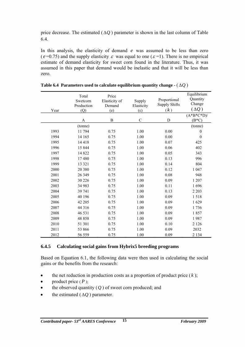
price decrease. The estimated ( Q∆ ) parameter is shown in the last column of Table 6.4. In this analysis, the elasticity of demand e was assumed to be less than zero ( =0.75) and the supply elasticity e ε was equal to one (ε =1). There is no empirical estimate of demand elasticity for sweet corn found in the literature. Thus, it was assumed in this paper that demand would be inelastic and that it will be less than zero. Table 6.4 Parameters used to calculate equilibrium quantity change - ( ) Q∆

Year

Total Swetcorn

Production (Q)

Price Elasticity of

Demand (e)

Supply Elasticity

(ε)

Proportional Supply Shifts

( ) k

Equilibrium Quantity Change ( ) Q∆

A B C D (A*B*C*D)/

(B*C) (tonne) (tonne)

1993 11 794 0.75 1.00 0.00 0 1994 14 165 0.75 1.00 0.00 0 1995 14 418 0.75 1.00 0.07 425 1996 15 844 0.75 1.00 0.06 402 1997 14 822 0.75 1.00 0.05 343 1998 17 480 0.75 1.00 0.13 996 1999 13 321 0.75 1.00 0.14 804 2000 20 380 0.75 1.00 0.12 1 047 2001 26 349 0.75 1.00 0.08 948 2002 30 226 0.75 1.00 0.09 1 207 2003 34 983 0.75 1.00 0.11 1 696 2004 39 741 0.75 1.00 0.13 2 203 2005 40 196 0.75 1.00 0.09 1 518 2006 42 205 0.75 1.00 0.09 1 629 2007 44 316 0.75 1.00 0.09 1 736 2008 46 531 0.75 1.00 0.09 1 857 2009 48 858 0.75 1.00 0.09 1 987 2010 51 301 0.75 1.00 0.10 2 126 2011 53 866 0.75 1.00 0.09 2032 2012 56 559 0.75 1.00 0.09 2 134

6.4.5 Calculating social gains from Hybrix5 breeding programs Based on Equation 6.1, the following data were then used in calculating the social gains or the benefits from the research: • the net reduction in production costs as a proportion of product price ( ); k• product price ( P ); • the observed quantity (Q ) of sweet corn produced; and • the estimated ( ) parameter. Q∆


Table 6.5 shows the social gains and royalties from the breeding research that resulted in the release of Hybrix 5. All values are expressed in 2006 dollars and a rate of 5 per cent was used to discount past and present values. The data in Table 6.5 presents the project benefits which includes the social gains plus royalties from the beginning of project up to 2006. Royalties were considered as benefits and were added in an annual basis to the social gains calculated. At the same time the increased cost of seed was included in the adoption costs. Table 6.5 Social gains from the adoption of the Hybrix5 sweet corn cultivar (1993-

06)

Year Proportional Supply Shifts

( ) kReal Price

( P )

Total Swetcorn

Production (Q )

Equilibrium Quantity Change ( Q∆ )

Social Gains ( ) SG Royalties

A B C D (A*B*C)-0.5*(A*B*D)

($/tonne) (tonne) (tonne) ($) ($) 1993 0.00 850.06 11 794 0 0 0 1994 0.00 694.58 14 165 0 0 0 1995 0.07 757.09 14 418 425 697 637 0 1996 0.06 602.95 15 844 402 513 040 0 1997 0.05 504.74 14 822 343 352 125 0 1998 0.13 735.67 17 480 996 1 587 051 86 230 1999 0.14 951.41 13 321 804 1 662 774 32 555 2000 0.12 537.12 20 380 1 047 1 188 348 68 204 2001 0.08 787.81 26 349 948 1 638 733 48 543 2002 0.09 797.58 30 226 1 207 2 111 231 83 929 2003 0.11 670.53 34 983 1 696 2 488 949 82 844 2004 0.13 576.74 39 741 2 203 2 776 148 187 273 2005 0.09 683.83 40 196 1 518 2 281 420 87 443 2006 0.09 774.20 42 205 1 629 1 525 805 84 074

Table 6.6 presents all the data from Table 6.5 together with the estimates of the benefits from 2007 up to 2012. This additional data were included because the project is still ongoing and will continue to have benefits in the future.


Table 6.6 Social gains from the adoption of the Hybrix5 sweet corn cultivar (1993-12)

Year Proportional Supply Shifts

( ) kReal Price

( P )

Total Swetcorn

Production (Q )

Equilibrium Quantity Change ( Q∆ )

Social Gains ( ) SG Royalties

A B C D (A*B*C)-0.5*(A*B*D)

($/tonne) (tonne) (tonne) ($) ($) 1993 0.00 850.06 11 794 0 0 0 1994 0.00 694.58 14 165 0 0 0 1995 0.07 757.09 14 418 425 697 637 0 1996 0.06 602.95 15 844 402 513 040 0 1997 0.05 504.74 14 822 343 352 125 0 1998 0.13 735.67 17 480 996 1 587 051 86 230 1999 0.14 951.41 13 321 804 1 662 774 32 555 2000 0.12 537.12 20 380 1 047 1 188 348 68 204 2001 0.08 787.81 26 349 948 1 638 733 48 543 2002 0.09 797.58 30 226 1 207 2 111 231 83 929 2003 0.11 670.53 34 983 1 696 2 488 949 82 844 2004 0.13 576.74 39 741 2 203 2 776 148 187 273 2005 0.09 683.83 40 196 1 518 2 281 420 87 443 2006 0.09 774.20 42 205 1 629 1 525 805 84 074 2007 0.09 700.57 44 316 1 736 1 381 335 33 629 2008 0.09 700.57 46 531 1 857 1 381 335 33 629 2009 0.09 700.57 48 858 1 987 1 381 335 33 629 2010 0.10 700.57 51 301 2 126 1 381 335 33 629 2011 0.09 700.57 53 866 2032 1 381 335 33 629 2012 0.09 700.57 56 559 2 134 1 381 335. 33 629

7. Results Figure 7.1 shows the exponential increase in gains as the Hybrix5 seeds are adopted and then soon after the ceiling is reached around 2004, social benefits declined.

-2000000

0

2000000

4000000

6000000

8000000

10000000

12000000

Social Gains Net Social Benefits Costs

Figure 7.1 Social gains, net social benefits and costs (1969 to 2012)


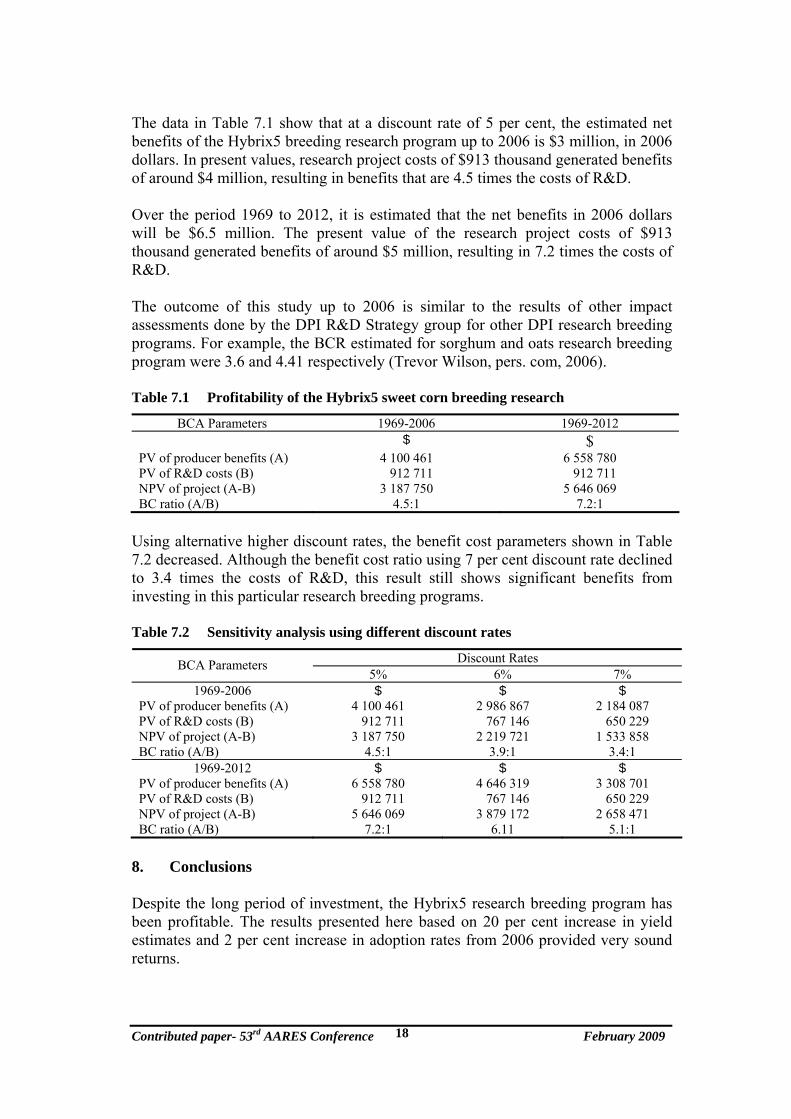
The data in Table 7.1 show that at a discount rate of 5 per cent, the estimated net benefits of the Hybrix5 breeding research program up to 2006 is $3 million, in 2006 dollars. In present values, research project costs of $913 thousand generated benefits of around $4 million, resulting in benefits that are 4.5 times the costs of R&D. Over the period 1969 to 2012, it is estimated that the net benefits in 2006 dollars will be $6.5 million. The present value of the research project costs of $913 thousand generated benefits of around $5 million, resulting in 7.2 times the costs of R&D. The outcome of this study up to 2006 is similar to the results of other impact assessments done by the DPI R&D Strategy group for other DPI research breeding programs. For example, the BCR estimated for sorghum and oats research breeding program were 3.6 and 4.41 respectively (Trevor Wilson, pers. com, 2006). Table 7.1 Profitability of the Hybrix5 sweet corn breeding research

BCA Parameters 1969-2006 1969-2012 $ $

PV of producer benefits (A) 4 100 461 6 558 780 PV of R&D costs (B) 912 711 912 711 NPV of project (A-B) 3 187 750 5 646 069 BC ratio (A/B) 4.5:1 7.2:1

Using alternative higher discount rates, the benefit cost parameters shown in Table 7.2 decreased. Although the benefit cost ratio using 7 per cent discount rate declined to 3.4 times the costs of R&D, this result still shows significant benefits from investing in this particular research breeding programs. Table 7.2 Sensitivity analysis using different discount rates

Discount Rates BCA Parameters 5% 6% 7%

1969-2006 $ $ $ PV of producer benefits (A) 4 100 461 2 986 867 2 184 087 PV of R&D costs (B) 912 711 767 146 650 229 NPV of project (A-B) 3 187 750 2 219 721 1 533 858 BC ratio (A/B) 4.5:1 3.9:1 3.4:1

1969-2012 $ $ $ PV of producer benefits (A) 6 558 780 4 646 319 3 308 701 PV of R&D costs (B) 912 711 767 146 650 229 NPV of project (A-B) 5 646 069 3 879 172 2 658 471 BC ratio (A/B) 7.2:1 6.11 5.1:1

8. Conclusions Despite the long period of investment, the Hybrix5 research breeding program has been profitable. The results presented here based on 20 per cent increase in yield estimates and 2 per cent increase in adoption rates from 2006 provided very sound returns.


In this report only producer benefits were quantified. Consumer benefits (i.e. increased demand for sweet corn due to improved taste - sweetness) were not included in this analysis due to the absence of data. They could, however, constitute significant benefits to the program. In spite of these conservative assumptions, the benefits of the release of Hybrix5 in 1995 are expected to continue to flow from it for considerable time. The investment into this research could produce a net present value of around $3 million and a benefit cost ratio of 4.5:1. 9. References Alston, J.M., Norton, G.W. and Pardey, P.A. 1998, Science Under Scarcity, Cab International , United Kingdom. Martin, I. F.2005, Breeding for Disease and Insect Resistance in Super-Sweet Corn: Final Report for VG 00073, Queensland Department of Primary Industries and Fisheries. Masters, W.A., Coulibaly, B., Sanogo, D., Sidibe, M. and Williams, A. 1996, The Economic Impact of Agricultural Research: A Practical Guide, Department of Agricultural Economics, Purdue University.


an ex post economic analysis impact of hybrix 5 sweet...

Documents