An Evolutionary Game Theory Explanation of ARCH Effects

William R. Parke1

Department of EconomicsUniversity of North CarolinaChapel Hill, NC 27599

George A. Waters2

Department of EconomicsIllinois State UniversityNormal, IL 61790-4200

June 14, 2006

1parke@email.unc.edu2gawater@ilstu.edu

Abstract

While ARCH/GARCH equations have been widely used to model financial market data, formalexplanations for the sources of conditional volatility are scarce. This paper presents a model withthe property that standard econometric tests detect ARCH/GARCH effects similar to those foundin asset returns. We use evolutionary game theory to describe how agents endogenously switchamong different forecasting strategies. The agents evaluate past forecast errors in the context ofan optimizing model of asset pricing given heterogeneous agents. We show that the prospects fordivergent expectations depend on the relative variances of fundamental and extraneous variablesand on how aggressively agents are pursuing the optimal forecast. Divergent expectations are thedriving force leading to the appearance of ARCH/GARCH in the data.

JEL Classification: C22, C73, G12, D84

Keywords:ARCH, autoregressive conditional heteroskedasticity, evolutionary game theory, ra-tional expectations,

Corresponding Author: William R. Parke, Department of Economics, University of NorthCarolina, Chapel Hill, North Carolina, 27516. 919-966-5393 (voice) 919-966-2383 (messages),919-966-4986 (fax), parke@email.unc.edu.

The goal of volatility analysis must ultimately be to explain the causes of volatility.While time series structure is valuable for forecasting, it does not satisfy our need toexplain volatility. .... Thus far, attempts to find the ultimate cause of volatility are notvery satisfactory.

- Robert Engle (2001)

Few models are capable of generating the type of ARCH one sees in the data. .... Mostof these studies are best summarized with the adage that “to get GARCH you need tobegin with GARCH.”

- Adrian Pagan (1996)

1 Introduction

ARCH/GARCH models have been used to describe the behavior of inflation, interest rates and

exchange rates1, and they have become the standard tool for analyzing returns in financial mar-

kets2. Despite the widespread empirical successes of ARCH/GARCH models, discovering under-

lying mechanisms that lead to time-varying volatility has proved to be an elusive goal.

We propose that time-varying volatility is a natural feature of models with forward-looking

agents. Our key condition is that agents are not constrained by assumption to agree on a single

expectation. Instead, we apply recent developments in evolutionary game theory to explain how

forward-looking agents might choose among differing forecasts. We assume that information arrives

uniformly over time so that changes in volatility are due entirely to agents’ behavior. Furthermore,

our agents do not set out simply to invent ARCH. They use ideas drawn from the literature on

rational expectations to choose among forecasts based on what they perceive to be fundamentals.

We establish conditions under which ARCH effects will be a normal feature of the resulting data.

The mechanism generating time-varying volatility has a general formulation. Evolutionary

game theory describes how fractions xt = (x1,t, ..., xk,t) of the population using forecasting strategies

st = (s1,t, ..., sk,t) evolve according to the performances of the strategies. An asset pricing model

then shows how the price yt depends on the fractions xt and other information Θt so that1Bollerslev (1986) examines inflation dynamics with a GARCH model. Engle, Lilien and Robins (1987) use the

ARCH in mean model to study yield curve issues. Diebold and Nerlove (1989) use a multivariate ARCH model toanalyze exchange rates.

2Engle (2001) provides a recent account of the methodology.

1

yt = y (xt,Θt). The fractions xt are taken to be known and fixed before yt is realized. We divide

Θt into information Ωt available to agents before yt is realized and all other information εt. The

model generating yt can then be written in the form

yt = y (xt,Ωt, εt) . (1)

After agents observe yt, they choose strategies for period t + 1, updating xt using a procedure of

the form

xt+1 = g(xt, yt,Ωt). (2)

Given this structure, the variance of the asset price can generally be written as

V (yt|xt,Ωt,Σt) = h (xt,Ωt,Σt) , (3)

where Σt is a measure of the volatility of εt. To clarify the source of conditional heteroskedasticity,

we assume that Σt is constant. The variance of yt will not, however, be constant if it depends on

the mix xt of agents’ strategies.

We demonstrate that ARCH effects can appear to be important in an empirical model for yt if

the econometrician does not take into account heterogeneity. A typical representative agent model

for yt, for example, would omit xt from (1) leaving

yt = y0 (Ωt, εt) .

The corresponding representative agent model of the conditional variance (3) would reduce to

V 0(yt|Ωt,Σt) = h0 (Ωt,Σt) . (4)

Standard econometric tests may well diagnose that the representative agent model (4) leaving out

the fractions xt has ARCH, making it appear to be necessary to account for changes over time

in Σt. We provide specific simulations that illustrate how apparent ARCH can be an artifact of

ignoring heterogeneous expectations.

2

These ARCH effects take place in a standard mean-variance optimization model of asset prices

extended to an environment with heterogeneous agents. Brock and Hommes (1998) develop the

theoretical basis for this model. They apply the model in an environment with multiple trader

types who use an assortment of linear forecasting rules. Brock, Hommes and Wagener (2005)

and Gaunersdorfer, Hommes, and Wagener (2003) extend these results.3 Other studies with het-

erogeneous expectations include Chiarella and He (2002), DeGrauwe (1993) and DeLong, Shleifer,

Summers and Waldmann (1990). Our study differs in that we focus on agents pursuing goals set

forth in the literature on rational expectations.

Our specific example features agents choosing among three forecasting strategies. A fundamen-

talist uses only expected future dividends to form his forecast. A mystic uses fundamentals, but

may also experiment with other extraneous information because, perhaps, there is some uncertainty

about what belongs in the fundamentals. A reflectivist incorporates all available information about

agents’ expectations, calculating the average expectation using population share weights.

We implement the procedure for updating agents’ choices of forecasting strategies (2) by having

agents switch to strategies that have exhibited lower squared forecast errors. The switching

probabilities are determined by the evolutionary dynamic of Hofbauer and Weibull (1996). That

dynamic allows for a nonlinear weighting function in the forecast evaluation. We add an important

dimension to our analysis by using the nonlinearity to parameterize how aggressively agents switch

forecasts.

Standard econometric tests applied to simulated data confirm that the extent of ARCH effects

depends on agent aggressiveness and on the variance of the potential extraneous element that

might enter the mystical forecast. If the latter variance is small relative to the variance of the

fundamentals or if agents are not very aggressive, then the asset price tends to follow fundamentals

nearly all the time. If the variance of the extraneous element is larger and agents are more

aggressive, then asset prices show occasional bubble behavior and both Engle’s (1982) test for

ARCH and estimates of a GARCH(1,1) model support the conclusion that the data can be described

as ARCH/GARCH for many of the simulations.

The role of heterogeneity has been noted in other related contexts with boundedly rational3Hommes (2006) surveys these and related models.

3

forecasting strategies. Lux and Marchesi (2000) construct an asset market with fundamentalists

and two different types of chartists, who respond to trends in the data. The switching probabilities

between the two strategies are determined by a modified discrete choice model that allows for slug-

gish adjustment. Their model shows that switching between strategies can produce ARCH effects

for certain parameter values. Föllmer, Horst and Kirman (2005) show the existence of bubbles,

but also show the existence of limiting distributions of asset prices in a discrete choice model with

forecasting strategies put forward by ‘gurus’ that could include chartists and fundamentalists. In

a similar framework, Gaunersdorfer and Hommes (2005) derive theoretical results indicating the

presence of bubbles and volatility clustering.

LeBaron, Arthur and Palmer (1999) study the time series features of a simulated asset market

and show the existence of ARCH effects and many other features of financial market data. They use

a computational approach with many trader types introduced throughout the simulation according

to a genetic algorithm. They find that the evidence of ARCH effects is much stronger in an

environment they term fast learning than it is given slow learning.

The focus in this paper on the possibility of heterogeneous forecasts stands in contrast to those

who argue that martingale solutions should be ruled out according to criteria such as transversality

(see Cochrane (2001) p. 27), minimum state variables (McCallum (1983, 1997)), and expecta-

tional stability (Evans and Honkapohja (2001)).4 In our context, the importance of the martingale

solutions depends on the parameter values and, while convergence to a single expectation is pos-

sible under some conditions, we establish the range of parameter values for which the martingale

solutions are an important feature. Using another approach that defines stability according to

rationalizability of strategies, Evans and Guesnerie (2003) show convergence to the minimum state

variables solution with homogeneous agents, but they also show instability in the case of heteroge-

neous agents.

The literature on convergence to rational expectations along the lines of least squares learning

(Grandmont (1998) and Marcet and Sargent (1989), for example) is also concerned with multiple

rational expectations equilibria. Woodford (1990) and Howitt and McAfee (1992) establish the4Evans and Honkapohja (2001) also discuss the possibility that bubble solutions might be learnable if agents use

a sufficiently complicated model to form expectations.

4

possibility of learning sunspot equilibria given accidental correlations between sunspots and fun-

damentals.5 While these papers focus on agents learning model parameters over time, our agents

know the parameters and are choosing among forecasts constructed from the multiple solutions to

the model.

den Haan and Spear (1998) explain conditional volatility in real interest rate fluctuations.

They construct an optimizing model where agents hold savings in the form of bonds. Agents are

heterogeneous, as in the present paper, and receive idiosyncratic shocks. Volatility clustering arises

due to borrowing constraints that vary across the business cycle.

The organization of the paper is as follows. Section 2 develops the asset pricing model with

heterogeneous agents. Section 3 and 4 describe the different forecasting strategies and their squared

forecast errors. Section 5 shows how agents’ choices of strategies evolve over time. Section

6 establishes how convergence of expectations depends on assumptions about agents’ beliefs and

willingness to consider new information. Section 7 describes the simulation methodology used in

the remainder of the paper. Section 8 provides examples and compares the simulations to some

stylized facts. Section 9 presents econometric analysis of the simulations using a GARCH(1,1)

model. Section 10 concludes.

2 Asset Pricing with Heterogeneous Agents

This section develops an optimizing model of asset pricing with heterogeneous agents based on

Brock and Hommes (1998). They extend a standard asset pricing model to the situation where

agents can have heterogeneous beliefs about future prices. Agents are myopic, mean-variance

optimizers who can choose between a risky asset and a riskless asset with gross rate of return R.

An agent’s wealth Wt evolves according to

Wt+1 = RWt + (yt+1 + dt+1 −Ryt) zt,

where yt is the price of the risky asset, dt is the dividend payment, and zt is the number of shares

of the risky asset purchased by the agent at time t. The asset price and dividend process are5Timmermann (1994) argues that feedback from lagged variables into dividends rules out rational bubbles.

5

stochastic so agents do not have precise knowledge of yt+1 or dt+1 when making decisions about

zt.

Agents may have heterogeneous expectations. For an agent of type j, let fj,t (Wt+1) be the

expectation of wealth conditional on the information available at time t, and let Vj,t (Wt+1) be the

perceived variance of Wt+1. Assume that the demand for shares zj,t by agents of type j maximizes

fj,t (Wt+1)− a2Vj,t (Wt+1) , (5)

where the parameter a denotes the level of risk aversion. If the perceived conditional variance

Vj,t (yt+1 + dt+1 −Ryt) for per share excess returns is the same constant σ2r for all agent types,then the demand for shares by agents of type j is given by

zj,t =

µ1

aσ2r

¶fj,t (yt+1 + dt+1 −Ryt) .

Summing the demand over the n types of agents, where the fraction of the population of type j is

xj,t, and equating total demand to a constant supply zs per investor yields the following condition

for the price of the risky asset

Ryt =nXj=1

xj,tfj,t (yt+1 + dt+1)−C, (6)

where C = aσ2rzs functions as a risk premium. This equation is analogous to Brock and Hommes’

(1998) equation (2.7).

We retain their assumption that the conditional variance σ2r of the per share excess returns is

constant. If agents were to expect bubbles, σ2r could be higher, but the results remain the same for

any constant σ2r. More sophisticated agents could try to estimate an ARCH model every period

to anticipate changes in volatility, causing σ2r to vary over time and across agents, but in order

to focus exclusively on ARCH effects that arise from heterogeneity in the forecasting strategies,

we rule out such behavior. It seems likely that variation in σ2r would add to rather than reduce

conditional volatility.

The pricing condition for agents with homogeneous rational expectations provides a useful

6

benchmark for asset pricing given heterogeneous expectations (6). If all agents were of a single

type, then yt would follow

Ryt = Et (yt+1 + dt+1)− C (7)

The bubble-free solution to this equation is yt = y∗t , where

y∗t =∞Xs=1

αsEtdt+s −µ

α

1− α

¶C (8)

and α = R−1. The self-fulfilling nature of expectations, however, admits the class of solutions

yt = y∗t + α−tmt, (9)

where mt is a martingale that we will express as mt = mt−1+ ηt for an i.i.d., mean zero stochastic

process ηt with variance σ2η. Requiring the variance of ηt to be constant is not necessary to satisfy

(7), but we want to rule out conditional volatility in the martingale innovation or in the dividend

innovation as sources of conditional volatility in the asset price.

To focus attention on the effects of choosing among forecasting strategies, we retain the key

underlying assumption of Brock and Hommes (1998) that agents have common beliefs about the

dividend process so that y∗t is common knowledge. We also take the realized martingale mt−1 to

be common knowledge although agents will disagree about whether it should be used to predict yt.

3 Strategies

The organization of this section and the next reflects the sequential process agents follow to deter-

mine yt. They begin period t with the vector of fractions xt already determined. Information Ωt

then arrives, and they compute forecasts for period t+ 1. These forecasts, given the asset pricing

model in the previous section, determine their share positions and, hence, the price yt. Once yt is

realized, they can compute forecast errors for the forecasts made in period t − 1. They then use

an evolutionary game theory mechanism to decide on fractions xt+1 for period t+ 1.

This section postulates three possible strategies for forecasting the asset price yt. The vector of

7

fractions following the three strategies will be denoted xt = (βt, γt,λt). The forecasting strategies

differ in two ways. Agents are not immediately certain whether newly proposed types of information

are fundamental or extraneous, and they differ in the extent to which they attempt to exploit

knowledge of other agents’ expectations.

A fraction γt of the population uses (8) to form the fundamentalist forecast

fγ,t(yt+1) = Ety∗t+1 (10)

Agents following fundamentals base their forecast solely on expected future dividends, ruling out

forecasts that involve the martingale mt. A fraction λt of the population uses a mystical forecast

fλ,t(yt+1) = Ety∗t+1 + α−t−1mt (11)

based on a martingale solution of the form (9). The basis for allowing agents to follow a martingale

solution is, of course, a critical issue.

Some researchers exclude such solutions on the basis of a transversality condition or similar

criterion (see Cochrane (2001) or other references in the introduction). These arguments require

strong assumptions about the information available to the agents. Recognizing that mt is, in fact,

a martingale and not stationary data is a classic econometric problem with the characteristic that

agents cannot know with certainty, on the basis of a finite data sample, that mt is nonstationary

and that a transversality condition is violated. Furthermore, the predictive properties of mt may

well be uncertain in finite samples. Later results in this paper show that, given the randomness of

sample correlations, forecasting strategies based on extraneous martingales can outperform other

strategies over the short term. Therefore, while agents may indeed rule out martingales in the

long run, ruling out martingales in finite data samples is another matter.

A martingale might well appeal to agents trying to follow fundamentals. Suppose mt is a

new idea (the impact of the Internet on commerce or the influence of sunspots6, for example) that

might or might not be a revision to the set of fundamentals. If mt is in fact a spurious martingale,6Typically, sunspot equilibria can be constructed in a model with martingale solutions. See Farmer (1999, Chapter

10) for a full discussion.

8

agents attempting to choose between (10) and (11) will eventually reject (11), but the process of

evaluating and rejecting (11) on the basis of empirical evidence may take some time. We diverge

here from the sunspot literature in that we assume that only a portion of the agents adopt the

sunspot forecast while others stick with the fundamentalist forecast.

For our third forecasting strategy, agents give primary attention to anticipating the choices of

others in a manner reminiscent of Keynes’ (1935) “beauty contest” interpretation of predicting

stock prices. We refer to this third forecast as the reflective forecast because it simply reflects

the views of others without attempting to consider the intrinsic value of the asset. Formally, we

assume that the reflective forecast is an average of the other two forecasts, weighted according to

their relative popularity. That is,

fβ,t(yt+1) = ntfλ,t(yt+1) + (1− nt) fγ,t(yt+1), (12)

where

nt =λt

λt + γt.

The reflective forecast can be expressed in terms of fundamentals and the martingale by substituting

(10) and (11) into (12) to obtain

fβ,t(yt+1) = Ety∗t+1 + α−t−1ntmt. (13)

The martingale thus influences the reflective forecast to the extent that the fraction nt of the

other agents are following the mystical forecast. If nt = 0 or nt = 1, then the reflective forecast

will numerically match the dominating forecast.7 The reflective forecast (13) differs from perfect

foresight because y∗t+1 −Ety∗t+1 and α−t−1nt+1mt+1 − α−t−1ntmt are not known in period t. The

reflective forecast brings to the system the notion of taking into account the expectations of other

agents, which is an important element of rational expectations.

The motive for agents to include the reflective forecast among the strategies they consider might

be some instinctive belief in the possible merit of averaging across available forecasts. An average7The reflective forecast is not well-defined for λt = γt = 0, but, as we explain in Section 6, that case is not the

focus of this paper.

9

is an obvious statistic to compute so it would not be be surprising if agents did the calculation.

In the next section we give this intuition a mathematical foundation by showing that, in every

period, the payoff to the reflective forecast is greater than or equal to the average payoff to the

other forecasts. Unless the fundamentalist and mystical forecasts happen to be numerically equal

(because mt = 0), the reflective forecast is guaranteed to have an above average payoff.8

The information requirements for these strategies differ somewhat, but to make switching strate-

gies possible we assume that all agents have access to the same information, including expected

dividends and the martingale. While the knowledge of the fractions βt, γt, and λt needed to

implement the reflective forecast might come from direct observation of other agents, that is not

necessary. The fractions change over time according to updating equations, given below as (24),

that are functions of the payoffs. Given that the agents know the payoffs and a starting point for

the fractions, they can recursively calculate the fractions over time just as we do in our simulations

later in this paper.9

Knowledge of the fractions βt, γt, and λt is easier to justify under the alternative interpretation

that there are many agents, but only three forecasters. Only the forecasters need to know how to

calculate a forecast. The agents simply choose among the available forecasts. Föllmer, Horst, and

Kirman (2005) make a similar distinction between agents and “gurus.”

The realized asset price (6) can be written as

yt = α(γtfγ,t(yt+1) + λtfλ,t(yt+1) + βtfβ,t(yt+1) +Etdt+1 − C).

Using (12) to express γtfγ,t(yt+1) + λtfλ,t(yt+1) in terms of fβ,t(yt+1) yields

yt = α(fβ,t(yt+1) +Etdt+1 − C),

which emphasizes that the reflective forecast does summarize the available information in deter-8 If mt = 0, then At = 0 in equation (20) below.9 It is beyond the scope of this paper, but one might consider the situation where the reflective forecast is based

on agent fractions estimated with some imprecision. For example, a loose interpretation of the updating equations(24) is that the fraction following a strategy can be estimated from its recent payoffs.

10

mining yt. Substituting (13) and noting that y∗t satisfies (7) yields

yt = y∗t + α−tntmt. (14)

The market price yt deviates from the price y∗t implied by the true fundamentals to the extent that

a nonzero fraction nt of the agents not following the reflective forecast are in fact following the

mystical forecast.

4 Evaluating Forecasts

Once yt is realized, agents are in a position to evaluate their current strategies, and there are

several possible criteria.10 We adopt the squared error criterion in light of its long tradition in

the econometrics literature for evaluating forecasts. LeBaron et. al. (1999) make the same choice.

Brock and Hommes (1998), on the other hand, use current realized trading profits. They also

suggest a more general weighted average of trading profits that includes accumulated wealth as

another case. Hommes (2001, p. 156) shows that the trading profits criterion does not take into

account risk, but that the squared error criterion can be derived from the utility function (5) for a

mean-variance optimizing risk averse agent. Gaunersdorfer, Hommes, and Wagener (2003) replace

the trading profits payoff in Brock and Hommes (1998) with a squared error payoff function and

derive qualitatively similar results.

We assume that agents attempt to forecast dt + yt rather than just yt because dt + yt is the

total return to holding an asset with price yt−1 in period t − 1. The agents share the common

expectation Et−1dt for dt so their forecasts for dt are identical. Using (10), (11), and (13), the

forecasts of yt from period t− 1 are given by:

fγ,t−1(yt) = Et−1y∗t ,

fλ,t−1(yt) = Et−1y∗t + α−tmt−1,

fβ,t−1(yt) = Et−1y∗t + α−tnt−1mt−1.10Blume and Easley (1992) discuss some issues involved in choosing payoff functions in the context of an evolutionary

study of asset pricing. They are concerned with long run survival of strategies.

11

The reflective forecast error can be decomposed using (14) as Ut = Ft +Gt, where

Ft = dt + y∗t −Et−1(dt + y∗t ) (15)

is the innovation in the fundamentals and

Gt = α−t(ntmt − nt−1mt−1) (16)

is the innovation in the weighted martingale. Using the notation At−1 = α−tmt−1, the fundamen-

talist and mystical forecast errors can be expressed as Ut+nt−1At−1 and Ut− (1−nt−1)At−1. Welet σ2F denote the variance of Ft, and, to focus unambiguously on other sources of heteroskedas-

ticity, we assume this variance is constant over time. The process Ft will be serially independent

regardless of the structure of the dividend process.

The payoffs are the negatives of the squared forecast errors:

πβ,t = −U2t , (17)

πγ,t = −U2t − 2nt−1At−1Ut − n2t−1A2t−1, (18)

πλ,t = −U2t + 2 (1− nt−1)At−1Ut − (1− nt−1)2A2t−1. (19)

The terms involving At−1 appear because the realized price depends on At−1 to the extent that

some agents follow the mystical forecast. The differences in the squared forecast errors depend on

the product of At−1 and Ut and the square of At−1.

Any of the three forecasts could have the best payoff in a particular period, and the ordering

depends on the realizations of At−1 and Ut. The ordering πλ,t > πβ,t > πγ,t can occur if the term

2 (1− nt−1)At−1Ut in the payoff to mysticism is positive (the mystic has conjured a fortuitously

accurate forecast) and sufficiently large. Similarly, πγ,t > πβ,t > πλ,t can occur if the term

2nt−1At−1Ut is sufficiently negative. If At−1Ut is sufficiently small in absolute value, then πβ,t is

greater than both πγ,t and πλ,t.

The reflective forecast has a natural advantage that we can express in terms of the fitness of a

12

given strategy, which is the difference between a given strategy’s payoff and the population average

payoff. Using the period t− 1 population shares of agents following the forecasts that produce therealized payoffs in period t, the average payoff is πt = βt−1πβ,t + γt−1πγ,t+ λt−1πλ,t. The fitness

of the reflectivist forecast is given by

πβ,t − πt = (1− βt−1)nt−1 (1− nt−1)A2t−1 ≥ 0. (20)

The reflectivist payoff is thus unambiguously better than the average payoff.

The nature of the contest between fundamentalism and mysticism is captured by

πλ,t − πγ,t = 2At−1Ut − (1− 2nt−1)A2t−1. (21)

If fundamentalism has a large following (nt−1 is near zero), then the term involving A2t−1 favors

continued domination by fundamentalism. A large positive At−1Ut could, however, reverse this

tendency. Mysticism has a symmetric advantage if nt−1 is near one, and that advantage could be

reversed by a large negative At−1Ut.

5 Evolution

To translate the relative payoffs into changes in agents’ beliefs we adopt a behavioral process from

evolutionary game theory known as “imitation of successful agents.”11 The name emphasizes that

the payoffs of other agents affect an agent’s probability of switching strategies. This contrasts with

strategies where agents focus only on their own payoffs.

Imitation of successful agents can be developed within a more general model of how agents

review and change forecasting strategies. Let rj,t be the fraction of agents using forecast j who

review their choice of strategy at time t, and let pij,t be the probability that a reviewing agent using

forecast j in period t switches to forecast i in the next period. We let xt = (βt, γt,λt) denote the

vector of population shares, and we will use xi,t to reference the elements of this vector. If there11Björnerstedt and Weibull (1996), Hofbauer and Weibull (1996), and Weibull (1997) develop imitation of successful

agents. DeLong, Schleifer, Summer, and Waldman (1990) use another form of imitation in their noise trader model.

13

are k available forecasts, then the change in xi,t is given by

xi,t+1 − xi,t =kXj=1

rj,txj,tpij,t − ri,txi,t. (22)

This is a discrete time version of equation (4.25) in Weibull (1997). We assume that all agents

review every period regardless of the payoff so rj,t ≡ 1, but that the transition probabilities pij,tdepend on the performances of the strategies. Agents will tend to switch to strategies with better

payoffs, meaning lower squared forecast errors. We assume that agents arrive at the transition

probabilities using payoff weighting functions w (πi,t) to calculate

pij,t =w (πi,t)xi,t

wt, (23)

where wt =nPh=1

w (πh,t)xh,t. The transition probability pij,t into strategy i depends on its current

popularity xi,t and on its current payoff w (πi,t) relative to the population weighted average wt.

Substituting (23) into (22) with rj,t ≡ 1 yields the equation of motion for the population shares

xi,t+1 = xi,tw (πi,t)

wt. (24)

The specific dynamics of the system will depend on the functional form of w(·).In particular, the dynamics of the system depend on the convexity of the weighting function

w (π). If w (π) is linear, the evolution of the fractions xi,t follows the replicator dynamic as the

fractions change proportionally with the fitness (payoff relative to the population average) of a

given strategy. For example, if w(π) = τ + π for a constant τ , then (24) can be written as

xi,t+1 = xi,tτ + πi,tτ + πt

. (25)

Given (20), βt is monotone increasing, leaving no opportunity for the emergence of mysticism

because γt and λt will be forced to their minimum possible values. (For Case 2 and Case 3

discussed in the next section, γt + λt is small, but positive.) No finite value for τ can guarantee

that τ + πi,t and τ + πt in (25) are positive, however, and setting w(π) to some positive constant

14

κ if τ + πi,t ≤ κ does introduce a convexity into w(πi,t). A convex weighting function provides

conditions that can lead agents to adopt the mystical forecast. Simulations (not reported in this

paper) show that the prospects for heterogeneous expectations depend on the value of τ , which

determines how frequently the constraint τ + π ≥ κ is binding.

To explore the relation between convexity in the payoff weighting function and convergence of

expectations, we base our analysis in this paper on the exponential weighting function

w (π) = eθ2π, (26)

where θ parameterizes the convexity of the function. Compared to the linear weighting function

underlying the replicator dynamic, convexity of the weighting function means the population shares

change overproportionally with the fitness of the strategies12. In economic terms, greater convexity

of w (π) implies that agents are seeking out the best performing strategy more aggressively.

We derive in the appendix approximations for the equations of motion for βt and

nt = λt/(λt + γt) that qualitatively characterize how the properties of the updating functions

depend on the convexity θ. For βt, when the accumulated martingale innovations have not yet

made A2t−1 large, we have

βtβt+1

∼= 1− θ2(1− βt)nt−1 (1− nt−1)A2t−1(1− 2θ2U2t ). (27)

Note thatβtβt+1

< 1 implies that reflectivism’s share is increasing. The fraction βt following

reflectivism will fall, making it possible for fundamentalism or mysticism to gain followers if agent

aggressiveness θ and the squared forecast error U2t for the reflective forecast are sufficiently large.

The nature of the contest between the fraction λt following mysticism and the fraction γt

following fundamentalism can be seen in an approximation to the equation of motion for nt:

ntnt+1

∼= 1− 2θ2(1− nt)(At−1Ut + (nt−1 − 12)A

2t−1). (28)

This equation of motion inherits properties noted for the simple difference in the mystical and12Hofbauer and Weibull (1996) examine the specification of the weighting function in detail.

15

fundamental forecast payoffs (21). If nt−1 is near zero or one, then the factor nt−1 − 12 acts to

put the weight of the squared martingale A2t−1 toward reinforcing that value of nt−1. Reversing

that trend requires a large value for At−1Ut of the appropriate sign. For example, if nt−1 is less

than 12 , then mysticism gains relative to reflectivism if At−1Ut is a large positive number with

At−1Ut > −(nt−1 − 12)A

2t−1. (A symmetric result for gains in fundamentalism applies if nt−1 is

greater than 12 .) Mysticism thus gains overall if a large squared forecast error U2t in (27) causes

a decrease in reflectivism and a large product At−1Ut in (28) appears to show that the martingale

predicts the forecast error. The factor θ2 in both (27) and (28) causes the magnitude of the changes

to be in proportion to the square of agent aggressiveness θ. A greater value for θ2 reduces the

number of consecutive fortuitous martingale realizations it would take to propel mysticism to a

given popularity.

Imitation of successful agents differs from the evolutionary mechanism Brock and Hommes

(1997) refer to as the discrete choice model.13 That model, which is a close relative of the multino-

mial logit model, can be written as

xi,t+1 =w(πi,t)Pkj=1w(πj,t)

,

where w(πi,t) = eβπi,t and β is the “intensity of choice,” which is similar to our measure θ of agent

aggressiveness. A fraction xi,t cannot reach 0 under the discrete choice model although for high

levels of β the fractions can become very small. The steady states for this model will, therefore,

be interior to the simplex containing the vector xt. Convergence to homogeneous expectations is

not possible.

Imitation of successful agents (24), on the other hand, has the property that x1,t/x2,t decreases

if w(π1,t) < w(π2,t). Inferior strategies can be driven to zero popularity because xi,t+1 depends

on xi,t in (24). The factor xi,t appears because the transition probability in (23) depends on

popularity, as measured by xi,t. In fact, if pij,t = xi,t in (23), then we would have a model of pure

imitation, where agents choose a new strategy by randoming picking another agent and adopting13Brock and Hommes (1997) introduced the discrete choice model as a method for studying the evolution of

heterogeneous expectations in a cobweb model. They extend this approach to the asset pricing framework discussedhere in Brock and Hommes (1998). Chiarella and He (2002) is one of many extensions.

16

that person’s strategy. Imitation of successful agents, as generated by (23), assumes that agents

switching strategies consider both current payoffs and popularities. The latter can be thought of

as measuring the quality of a strategy’s previous payoffs because a strategy gains in popularity to

the extent it secures a series of favorable payoffs.

Considering the possibility of convergence to homogeneous expectations is thus reasonable under

imitation of successful agents. The central question will be whether that outcome is robust to the

introduction of small fractions of agents using alternative strategies.

6 Convergence of Expectations

We have constructed an evolutionary model of expectation formation in order to consider whether

expectations converge and, if they do not, to characterize the nature of the resulting heterogeneous

expectations. We will show that persistent heterogeneous expectations are more likely if agents

are more aggressive. Two additional features of agents’ behavior are important factors.

(i) Fundamentalism might have a special appeal because it is so widely cited by learned economists.

(ii) Agents might be willing to consider new information thought by some to help predict yt. We

analyze three cases.

Case 1: No Underlying Beliefs

If agents simply play the game as it is described to this point (without (i) and (ii) above), then

xt = (βt, γt,λt) will eventually cease changing when it reaches one of two edges of the simplex

∆ = (βt, γt,λt)|βt ≥ 0, γt ≥ 0,λt ≥ 0, and βt + γt + λt = 1. The evolution equation (24) showsthat xi,t = 0 implies xi,s = 0 for s ≥ t. That is, if a strategy has no followers, it cannot acquire any.On the edge where λt = 0 and on the edge where γt = 0, nonzero weights apply to the reflective

forecast and one other forecast. The two forecasts are numerically identical so there will be no

further change in xt = (βt, γt,λt). The edge where βt = 0 is not an absorbing state because the

fundamental and mystical forecasts will not be numerically equal and the evolution will continue

until λt = 0 or γt = 0. The outcome will thus be some combination of reflectivism and one other

strategy where the third strategy is extinct.14

14The reflective strategy is not well-defined at the point where (β, γ,λ) = (1, 0, 0), but the fractions cannot reach

17

This first case does not provide a very satisfying foundation for homogeneous expectations.

In the long run, the expectations will follow either the fundamental solution or the martingale

solution, but the outcome depends on the starting fractions and a period of stochastic movement

among strategies. Given the algebraic symmetry in (18) and (17), there is no meaningful difference

between fundamentalism and mysticism from the point of view of the game.

Case 2: Core Belief in Fundamentals and Averages

By augmenting the model with two assumptions about agents’ core beliefs, we can make a

strong case for convergence to fundamentals.

Condition 1 The fraction βt is bounded from below by the minimum βmin > 0.

Two arguments support the assumption that a core fraction βmin of the agents are willing to

stick with the reflective strategy regardless of particular realized payoffs. First, equation (20)

guarantees that the payoff to the reflective forecast is at least equal to the average payoff. Second,

if the process does converge to a steady state with a single dominant strategy, then the reflective

forecast will automatically match the winning forecast numerically, guaranteeing its followers the

maximum possible payoff. Case 1 is an example of this. While we do not have explicit costs of

evaluating or switching strategies, the reflective forecast avoids both while maintaining an above

average payoff at all times and matching whatever forecast is eventually dominant.

Condition 2 The fraction γt is bounded from below by the minimum γmin > 0.

We attribute the core following for fundamentalism to published research in economics. A large

literature in economics attempts to justify the assumption that agents will unanimously agree on

the fundamental solution to models with forward expectations. Countless papers simply impose

this assumption. We do not assume universal belief in the fundamentalist forecast, but we do

assume that some fraction γmin of the agents choose their strategy based on published economic

research and follow the fundamentalist forecast regardless of what other agents do.

Our goal with Case 2 is to consider the possibility of convergence to the fundamentalist expec-

tation without simply imposing the assumption that γmin = 1.00. In our simulation results, we

that point in Cases 2 and 3, which are the focus of this paper.

18

take both βmin and γmin to equal 0.05. We pick 0.05 to be small relative to 1.00, but large relative

to the precentage of the agents who consider the mystical forecast in Case 3 below.

For even these small figures, mysticism will eventually lose its appeal and the fractions will

move to the steady state where λt = 0. While mysticism can gain popularity when the martingale

accidentally forecasts fundamentals, any period of relatively small squared forecast errors will, ac-

cording to (27), drain followers from both mysticism and fundamentalism, increasing the following

of reflectivism. The limit of this process leaves a remaining core γmin = 0.05 of unyielding funda-

mentalists that outnumbers the remaining λmin = 0 followers of mysticism. It is thus the natural

advantage of reflectivism and the core of unyielding fundamentalists that lead to the collapse of

mysticism in the long run.

The mechanism that causes the eventual failure of mysticism is an important characteristic of

our model. In some models of rational bubbles, Evans (1992) and Hall, Psaradakis and Sola (1999),

for example, the bubble collapses with some exogenously given probability.15 The collapse in our

model occurs endogenously, given the natural tendency for the fraction βt following the relective

forecast to increase and given that we take γmin to be substantially larger than λmin because the

fundamental solution is prominently featured in published economics research. Furthermore, the

collapse of mysticism requires only that agents study squared forecast errors, not that they develop

some deeper theory about minimum state variables or expectational stability.

Case 3: Evaluating New Information

The central question we address in this paper is whether the convergence to the fundamentalist

forecast in Case 2 is robust to a very small fraction of the agents evaluating new information.

In particular, suppose the agents consider the mystical forecast, which is based on a martingale

solution. We assume that the agents cannot know with certainty that the martingale is extraneous.16

In our simulation results, we study the effects if λmin = 0.0001 of the agents consider the mystical

forecast. In practice, we choose λmin to be much lower than the other minima so that, if mysticism is

near its minimum, it has very little effect on the asset price and yt essentially follows the fundamental15Charemza and Deadman (1995) present an alternative model of speculative bubbles analogous to Evans (1992).

The explosive term enters additively in Evans (1992) and multiplicatively in Charemza and Deadman (1995).16Even if the agents intend to rule out nonstationary solutions, nonstationarity tests do not yield certainty in finite

samples.

19

solution. Our goal is to find out whether, even after a very minimal beginning, mysticism can gain

sufficient following to impact the system, causing bubble-like behavior and inducing ARCH effects

in the time series data. Our formal statement of this challenge to stability is

Condition 3 The fraction λt is bounded from below by the minimum λmin > 0. If this bound is

reached, the martingale restarts at mt = 0.17

Analyzing whether equilibria are robust to the introduction of small fractions of the population

using alternative strategies is a common topic in evolutionary game theory. Binmore, Gale and

Samuelson (1995) and Binmore and Samuelson (1999), in particular, consider the possibillity that

arbitrarily small “drift” in the population fractions can have large impacts on the outcome. Here,

we simulate the model while imposing λmin = 0.0001 to examine the stability of adherence to the

fundamental solution when a very small fraction of the agents consider extraneous information.

7 Simulation Methodology

The remainder of this paper examines the empirical properties of the per share excess return

Zt = dt + yt − α−1yt−1, (29)

which is a natural measure of investment performance. Expressing yt as (14) and noting that y∗t

satsifies (7) yields Zt = Ut + C, where Ut = Ft +Gt is the reflectivist forecast error given by (15)

and (16) and C is the risk premium that appears in (6). Because C is constant in this paper, the

per share excess returns are (up to a constant) equal to the reflectivist forecast errors.

One advantage of studying per share excess returns rather than percentage returns is that

our results are invariant to the dynamic structure of the dividend process. We can simulate

the serially independent innovations to fundamentals Ft without making assumptions about the

dividend process and without actually calculating dt, yt, and yt−1.1817An alternative would be have a new martingale start every period, but that would lead to a large and variable

number of strategies in a given period.18 In calculations not reported here we have checked the differences that might result from assuming a specific

dividend process in order to make possible direct calculation of dt, yt, and gross percentage returns (dt + yt −yt−1)/yt−1. Results for gross percentage returns very similar to those in Tables 1 and 2 for excess returns can beobtained if dividends are assumed to follow an AR(1) process with an autoregression parameter equal to 0.95.

20

The conditional volatility of excess returns Zt depends on three main parameters: agent ag-

gressiveness θ, martingale volatility ση, and the volatility of fundamentals σF . We adopt the

normalization σF = 1.0 so that the volatility of the fundamentals is fixed. Some normalization is

necessary because multiplying θ by a constant φ while dividing Ft, Gt, and At by φ would leave the

weighted payoffs (26) unchanged. The normalization σF = 1.0 has the intuitive appeal of holding

the properties of fundamentals fixed while focusing on agent behavior and on the nature of the

extraneous martingale.

Other parameters are fixed at reasonable values that are constant across simulations. These

parameter values include the agents’ risk aversion parameter a = 0.25, the discount factor α = 0.99,

and the total supply of shares per investor zs = 1.0.

All simulations begin at the potentially stable point where reflectivism has its maximum number

of followers given Conditions 2 and 3. The initial fraction λmin = 0.0001 of the population using

the mystical forecast is much lower than the other minima, γmin = 0.05 and βmin = 0.05. While

we assume that one agent in 20 is an unyielding believer in the true fundamentals, we assume that

only one agent in 10,000 is attracted to a mystical forecast under first consideration. The initial

minimum fraction following fundamentalism thus dominates the initial fraction following mysticism,

making the reflectivist forecast nearly identical to the fundamentalist forecast. These initial values

are intended to ensure that the ARCH effects in the simulated data do not arise spuriously from

the size of the initial fraction following mysticism.

If, after some initial increase, the following λt for the mystical forecast again falls to the minimum

λmin, we implement Condition 3 by allowing λt to remain at λmin and resetting the martingale to

mt−1 = 0. This effectively represents a new mystical forecast. The model in this paper could be

extended to include many different mystical forecasts operating simultaneously, but we focus on a

single mystical forecast for clarity. An alternative approach, which is common in the computational

finance literature (LeBaron (2000, 2006)) would be to regularly introduce new strategies into the

population.

21

8 Volatility Clustering and Excess Kurtosis

Volatility clustering and fat tails are two of the most striking properties of excess returns in financial

market data.19 In this section, we explore the relation between these phenomena on the one hand

and agent aggressiveness and the variance of the martingale innovation on the other.

Figures 1, 2, and 3 show typical realized simulations for the model. The top graph in each

figure is the realized share price.20 The second graph shows the per share excess return. The

bottom three graphs show the shares of the population using each strategy across time.

Figures 1 and 2 ilustrate the dramatic differences between cases where agents basically agree

on a single forecast and cases where agents hold heterogeneous, evolving expectations. Figure

1 (ση = 1.0, θ = 0.5) shows a case where mysticism plays no role. The population share for

mysticism remains at its minimum, and the asset price remains close to the fundamental solution.

Figure 2 (ση = 1.0, θ = 1.0) shows how mysticism becomes a factor when agents are more

aggressive. There are periods when mysticism succeeds in attracting adherents, becoming the

dominant strategy at times. Stretches of time when mysticism dominates often show bubble

behavior in the asset price and large deviations from zero in the excess returns. Such bubbles

do not, however, last indefinitely. As we note in Section 6, the unyielding fraction γmin following

fundamentals is much larger than the minimum fraction λmin for mysticism, and reflectivism has a

natural advantage. These two factors lead to an eventual collapse of mysticism.

Figure 3 (ση = 2.0, θ = 2.0) shows a further increase in martingale volatility sufficient to cause

briefer, but more decisive episodes of mysticism. Volatility clustering in the returns is quite evident

and occurs around short outbursts of mysticism. Engle (2001) suggests that clusters of large shocks

must be the result of news. We can interpret our simulations as agents temporarily responding to

a new variable, but quickly discarding it as irrelevant. Mysticism can gain a large following but it

usually lasts for less than 10 periods before it is rejected. Outbreaks of mysticism that last longer,

as shown in Figure 2, tend to occur for more moderate values of θ and ση.

To formally confirm the volatility clustering apparent in these figures, we also calculate Engle’s19Pagan (1996).20As we note in the previous section, we need the variance of the innovation to fundamentals, but not a specific

dividend process to calculate excess returns and the fractions βt, γt, and λt. To calculate realized share price for thegraph, we use the auxiliary assumption that dividends follow an AR(1) process with autoregression parameter 0.95.

22

(1982) test for ARCH in the simulated returns (29), setting the lag parameter to 5.21 The critical

value for Engle’s test for ARCH is 11.07. The test statistics for Figures 1, 2, and 3 are 2.68, 39.01,

and 62.83, respectively.

Table 1 gives a more comprehensive view of some features of the simulated data. The four panels

show degrees of agent aggressiveness, and the rows within the panels show degrees of martingale

volatility. Each entry in the first column shows the percentage of the sample runs, out of 10,000

trials, for which one would reject the null hypothesis of homoskedasticity using the 0.05 critical

value for Engle’s test with the lag parameter set to 5. Column 2 shows the average estimate of

the long memory parameter d for the Geweke and Porter-Hudak (1983) estimation procedure for

squared excess returns. Column 3 shows the average kurtosis over the trials. The three columns

on the right show the average percentage (over all trials and all periods) of the agents following

each of the three forecasting strategies.

The basic finding in Table 1 is that agent aggressiveness and martingale volatility both con-

tribute to the likelihood of diagnosing ARCH and excess kurtosis in the simulated data. Agent

aggressiveness, parameterized by the curvature of the payoff function, is clearly important. If the

parameter θ determining agent aggressiveness is less than 1.00, there is no evidence of ARCH for

any level of martingale volatility. For θ ≥ 1.00, however, ARCH is a dominant feature of the dataas agents aggressively switch forecasts searching for the optimal strategy.

For a fixed level of agent aggressiveness θ, Table 1 shows that mysticism is more likely to be

an important factor for a large ση. Small martingale innovations lead to small differences in the

payoffs ((17), (18) and (19)), making the likely gains in popularity for mysticism small even when

At−1 does match the sign of Ut. For a larger martingale innovation variance, fortuitious values for

At−1 have a greater chance of causing large differences in the payoffs and gains for mysticism.

The estimates of the long memory parameter for squared excess returns, on the other hand, show

no indication that long memory is an important feature of the simulations.22 Several sets of results

that are not reported in Table 1 also show no evidence of long memory. The serial correlation21Engle’s test is a joint test of the coefficients of the first k lags of the squared residuals in a regression on the

current squared residual. Calculations for a range of alternative values for k show that the results are not particularlysensitive to this parameter for our simulations.22Pagan (1996, p.30) notes the common finding of long memory in empirical squared excess returns.

23

coefficients for squared and absolute excess returns have the pattern that, in cases where the first-

order serial correlation is noticeably greater than zero, the higher order serial correlations drop

toward zero faster than is consistent with long memory. The long memory parameter estimates

for the absolute value of excess returns are similar to those for squared excess returns, but smaller.

For excess returns , the estimates of d are all very near zero.

The most striking feature of the population fractions in Table 1 is that the average percentage

following mysticism does not have to be very large to induce ARCH. For θ = 1.0, the average

fraction following mysticism is less than 0.015 in all cases even though the probability of rejecting

homoskedasticity is as high as 0.700. In no case in Table 1 does the average fraction following

mysticism exceed 0.12.

9 GARCH

A natural next step is to examine the simulated data that showed ARCH effects to see whether

it is well represented by a GARCH (Generalized ARCH) model. GARCH models, introduced by

Bollerslev (1986), are commonly used to examine financial market data and offer a useful extension

of the ARCH approach. We examine the simulated data with the GARCH(1,1) model that Engle

(2004) terms “the workhorse of financial applications.”23 This approach models the conditional

variance of the errors Et−1¡ε2t¢= σ2R,t as

σ2R,t = κ+ ϕσ2R,t−1 + ψε2t−1, (30)

where κ, ϕ, and ψ are constants. The conditional variance depends on the previous period’s

conditional variance and on the previous period’s squared error. The advantage of this specification

is its parsimony. It does not require multiple lags of ε2t , and it separates the effects of the long

term conditional variance σ2R,t−1 and the short term squared errors ε2t−1. Of course it is possible

to include further lags of either variable, but, as Engle (2001) notes, the GARCH(1,1) model has

proved sufficient for most financial market data.

Table 2 reports estimation results for GARCH(1,1) models for the data described for Table 1.23Bollerslev, Chou, and Kroner (1992) survey GARCH modeling in finance.

24

Following the organization of Table 1, each section of the table gives results for a given level of

agent aggressiveness, and each row summarizes the results for a given standard deviation of the

martingale innovation. Each row is calculated using 1,000 sample runs of 1,000 periods. All the

reported statistics are calculated for just those simulations for which Engle’s test rejects the null

of no ARCH, making the GARCH results conditional on a preliminary diagnosis of ARCH.

The estimate of ϕ is the best initial indication of whether the data is well represented by (30).

For those cases where Engle’s test rejects the null of no ARCH, Column 1 gives the conditional

probability that a significance test for the estimate of ϕ will reject the null of zero, implying that

the conditional variance is serially dependent. Columns 2 gives the mean of the estimates of ϕ for

the cases where H0 : ϕ ≤ 0 is rejected.We also report rejection probabilities for H0 : ψ ≤ 0 in Column 3. The probability in Column 3

is conditional on the Engle test rejecting the null of no ARCH and the test of ϕ rejecting H0 : ϕ ≤ 0.Column 4 shows the mean of the estimates of ψ where the null is rejected. Finally, we conduct

a diagnostic test (Enders (2004, p. 136)) for serial correlation in the squared residuals, using a

Ljung-Box Q test on the runs for which ϕ is significantly greater than zero. The final column

reports the percentage of the runs for which the Q test rejects the null of no serial correlation in

the squared error terms.

We draw two main conclusions from Table 2. First, as in Table 1, agent aggressiveness θ

and martingale volatility ση are both important in determining the relevance of a GARCH(1,1)

empirical model. For small values of these parameters, few trials are diagnosed as having ARCH

by Engle’s test and, for those few trials for which the null of no ARCH is rejected, the frequency of

rejecting H0 : ϕ ≤ 0 is modest. For larger values of θ and ση, the probability of rejectingH0 : ϕ ≤ 0is over 0.5 in several cases. For those cases, the probability of rejecting H0 : ψ ≤ 0 is near one andthe probability that the diagnostic test finds serial correlation in the squared residuals is near the

nominal 5% size of the test. For several rows in Table 2, therefore, there is a good chance that

standard econometric tests would support the conclusion that the data is GARCH(1,1).

Second, Table 2 hints at the empirical appeal of generalizing the basic ARCH/GARCH models.

At the highest level of agents aggressiveness θ = 4.0 and for the larger values of martingale volatility

ση, the results for Engle’s test in Table 1 are decisively in favor of ARCH. For those same parameter

25

values, Table 2 does not lend much support to fitting a GARCH(1,1) model. The probability of

rejecting H0 : ϕ ≤ 0 is relatively low, as is the mean of the significant estimates of the ARCH

autoregression parameter ϕ in the two rows for the larger values of ση. While the rejection

probabilities for the diagnostic test are not large for any rows of the table, the larger rejection

probabilities occur for the higher values of agent aggressiveness θ. These results point in the

direction of a more extensive search over the generalized family of ARCH models.

Overall, the results in Table 2 demonstrate that letting agents choose among competing fore-

casts can produce ARCH/GARCH effects that are very similar to those found in data for financial

markets. We can decompose the parameter combinations of martingale volatility and agent ag-

gressiveness into three regions. For low martingale volatility and/or low agent aggressiveness, the

process is nearly always at the fundamentalist solution. For somewhat higher martingale volatility

and/or agent aggressiveness, mysticism becomes an important factor, the data frequently exhibit

symptoms of ARCH, and a GARCH(1,1) model often fits the data very well. For very high martin-

gale volatility and very aggressive agents, Engle’s (1982) test for ARCH rejects the null hypothesis

decisively, but the volatility in the system cannot always be adequately modeled by a GARCH(1,1)

model. In this situation, econometricians committed to an ARCH approach would likely construct

a model more complex than GARCH(1,1).

10 Conclusion

While ARCH/GARCH models have proved to be extremely successful empirical econometric tech-

niques, explaining the underlying causes of conditional volatility in financial markets has been a

difficult challenge. This paper presents a formal model explaining how such effects arise endoge-

nously when forward-looking agents choose among forecasting strategies.

The leading candidate for the source of conditional volatility has long been news of some kind

(Engle (2001, 2004)). Our results are driven by the arrival of new information, but they do not

require any assumption that information arrives at nonuniform rates. We show instead that the

process of experimenting with and rejecting sources of information can be a key factor explaining

conditional volatility. In fact, our parameter specifying how aggressively agents search for the

26

optimal forecasting strategy is a primary factor in accounting for conditional volatility.

Our results do not require any radical departure from rationality. We consider only forward-

looking mean-variance optimizing agents who differ only because they choose among three forecast-

ing strategies that are all consistent with the notion of rational expectations. The fundamentalists

use the rational expectations solution dominant in that literature. Mysticism follows the same

principles, but mistakenly experiments with the idea that the martingale innovations are funda-

mental. Both fundamentalism and mysticism are, of course, only fully rational if they are adopted

by all agents. The reflectivists focus on this point and adopt a forecast taking full account of the

behavior of the other two groups of agents.

The characteristics of the realized asset price differ dramatically across parameter values. If

the martingale variance is small or agents are not very aggressive in pursuing the optimal fore-

casting strategy, agents tend to agree numerically on the fundamentalist forecast and there is little

evidence of volatility clustering. For larger martingale variances and/or more aggressive agents,

ARCH/GARCH effects appear in significant fractions of the sample runs.

Econometric tests of the simulated data in the latter cases detect ARCH and GARCH effects

similar to those found in financial market data. We test for ARCH using Engle’s (1982) test

and then estimate the GARCH(1,1) model often used in practice. For a range of martingale

volatility and a range of agent aggressiveness, the sample statistics indicate that the simulated

data is well represented by a GARCH(1,1) model. For the combination of a large martingale

innovation variance and very aggressive agents, the evidence points in the direction of ARCH, but

in a form more complicated than a GARCH(1,1) model. As we propose in the introduction to this

paper, these results confirm that empirical ARCH/GARCH effects can be an artifact of viewing

data generated by heterogeneous expectations from the perspective of a model that assumes a single

expectation.

One implication of these results is that a test for ARCH can be viewed as a specification test

for the assumption that agents agree on a single expectation. ARCH will be observed if the levels

of martingale volatility and agent aggressiveness are high enough to make divergent expectations

a common feature of the data. From this perspective, the widespread econometric evidence in

favor of ARCH/GARCH for variables such as inflation, interest rates, exchange rates, and returns

27

on financial assets presents a challenge to the assumption that agents in models explaining these

variables agree on a single expectation.

28

Appendix

To derive the approximate equations of motion (27) and (28), it proves convenient to turn (24)

upside-down to producexi,txi,t+1

=wt

w (πi,t).

For βt this becomes

βtβt+1

=βtexp(θ

2πβ,t) + γtexp(θ2πγ,t) + λtexp(θ

2πλ,t)

exp(θ2πβ,t),

which can be written as

βtβt+1

= βt + γtexp(θ2(πγ,t − πβ,t)) + λtexp(θ

2(πλ,t − πβ,t)).

A two-term Taylor series approximation to each exponential function (about At = 0) yields

βtβt+1

∼= 1 + γt(θ2(πγ,t − πβ,t)) + λt(θ

2(πλ,t − πβ,t)) +γt2(θ2(πγ,t − πβ,t))

2 +λt2(θ2(πλ,t − πβ,t))

2.

Substituting

πγ,t − πβ,t = −2nt−1At−1Ut − n2t−1A2t−1

and

πλ,t − πβ,t = 2 (1− nt−1)At−1Ut − (1− nt−1)2A2t−1

from (17), (18), and (19) introduces a variety of terms involving At−1 and Ut. We retain the terms

involving A2t−1 and A2t−1U2t . The terms involving At−1Ut cancel. We leave out the terms involving

A3t−1Ut on the grounds that their expectation is near zero.24 We leave out the terms involving

A4t−1 on the grounds that they will be dominated by the terms involving A2t−1 for small variances

of the martingale innovation, especially early in the history of the martingale.25 Our approximate24The weights in the martingale innovation in Gt change between period t−1 and period t, leaving open a tenuous

possibility of some correlation with the lagged martingale.25We consider values of ση as large as 4.0, and this approximation does not apply to such large martingale innovation

variances. This point has no effect on our results because the simulations use the complete nonlinear equations ofmotion, not the approximations in this appendix.

29

equation describing the motion of βt is thus

βtβt+1

∼= 1− (1− βt)(θ2nt−1 (1− nt−1)A2t−1 + 2θ4nt−1 (1− nt)A2t−1U2t ).

The equation of motion (28) for nt follows from

nt+1 =λtw(πλ,t)

λtw(πλ,t) + γtw(πγ,t).

If nt+1 > 0 and w(πλ,t) > 0, some rearrangement yields

ntnt+1

= 1 + (1− nt)µw(πγ,t)

w(πλ,t)− 1¶.

(If w(πλ,t) = 0, then nt+1 = 0.) If the payoff weight w(πγ,t) for fundamentalism is less than the

payoff weight w(πλ,t) for mysticism, then nt = λt/(γt + λt) increases. A one-term Taylor series

approximation about πβ,t for each exponential function yields

ntnt+1

∼= 1− 2(1− nt)w0(πβ,t)w(πβ,t)

(At−1Ut + (nt−1 − 12)A

2t−1).

The factor w0/w measures curvature of the payoff weighting function, which we identify as agent

aggressiveness. The potential for large changes in nt depends on this measure of agent aggressive-

ness.

30

References

Binmore, K., Samuelson, L., 1999. Evolutionary drift and equilibrium selection. Review of Eco-nomic Studies 66, 363-393.

Binmore, K., Gale, J., Samuelson, L., 1995. Learning to be imperfect: the ultimatum game.Games and Economic Behavior 8, 56-90.

Björnerstedt, J., Weibull, J.W., 1996. Nash equilibrium and evolution by imitation, in The Ratio-nal Foundations of Economic Behavior, K. Arrow, et. al., eds., Macmillan, London, 1996.

Blume, L.E., Easley, D., 1992. Evolution and market behavior. Journal of Economic Theory 58,9-40.

Bollerslev, T., 1986. Generalized autoregressive conditional heteroskedasticity. Journal of Econo-metrics 31(3), 307-327.

Bollerslev, T., Chou, R.Y., Kroner, K.F., 1992. ARCH modeling in finance: a review of the theoryand empirical evidence. Journal of Econometrics 52, 5-59.

Brock, W.A., Hommes, C.H., 1997. A rational route to randomness. Econometrica (65), 1059-1095.

Brock, W.A., Hommes, C.H., 1998. Heterogeneous beliefs and routes to chaos in a simple assetpricing model. Journal of Economic Dynamics and Control 22, 1235-1274.

Brock, W.A., Hommes, C.H., Wagener, F.O.O., 2005. Evolutionary dynamics in financial marketswith many trader types. Journal of Mathematical Economics 41, 7-42.

Charemza, W.W., Deadman, D.F., 1995. Speculative bubbles with stochastic explosive roots: thefailure of unit root testing. Journal of Empirical Finance 2, 153-163.

Chiarella, C., He, X., 2002. Heterogeneous beliefs, risk and learning in a simple asset pricing model.Computational Economics 19, 95-132.

Cochrane, J.H., 2001. Asset Pricing. Princeton University Press, Princeton, NJ.

DeGrauwe, P., 1993, Exchange Rate Theory: Chaotic Models of Foreign Exchange Markets. Black-well, Cambridge, MA.

DeLong, J.B., Shleifer, A., Summers, L.H., Waldmann, R.J., 1990. Noise trader risk in financialmarkets. Journal of Political Economy 98, 703-738.

den Haan, W.J., Spear, S., 1998. Volatility clustering in real interest rates: theory and evidence.Journal of Monetary Economics 41, 431-453.

Diebold, F.X., Nerlove, M., 1989. The dynamics of exchange rate volatility: a multivariate latent-factor ARCH model. Journal of Applied Econometrics 4, 1-22.

31

Enders, W., 2004. Applied Economic Time Series, Wiley, Hoboken, NJ.

Engle, R.F., 1982. Autoregressive conditional heteroskedasticity with estimates of the variance ofU.K inflation. Econometrica 50, 987-1008.

Engle, R.F., 2001. GARCH 101: the use of ARCH/GARCH models in applied econometrics.Journal of Economic Perspectives 15(4), 157-168.

Engle, R.F., 2004. Risk and volatility: econometric models and financial practice. AmericanEconomic Review 94(3), 405-420.

Engle, R.F., Lilien, D.M., Robbins, R.P., 1987. Estimating time varying risk premia in the termstructure: the ARCH-M model. Econometrica 55, 391-407.

Evans, G.W., 1992. Pitfalls in testing for explosive bubbles in asset prices. American EconomicReview 81, 922-30.

Evans, G.W., Honkapohja, S., 2001. Learning and Expectations in Macroeconomics. PrincetonUniversity Press, Princeton, NJ.

Evans, G.W., Guesnerie, R., 2003. Coordination on saddle path solutions: the eductive viewpoint— linear multivariate models. Macroeconomic Dynamics 7(1), 42-62.

Farmer, R.E.A., 1999. The macroeconomics of sulf-fulfilling prophecies, second edition. The MITPress, Cambridge, Massachusetts

Föllmer, H, Horst, U., Kirman, A., 2005. Equilibria in financial markets with heterogeneous agents:a probabilistic perspective. Journal of Mathematical Economics 41, 123-155.

Gaunersdorfer, A., Hommes, C.H., 2006. A nonlinear structural model for volatility clustering.Forthcoming in G. Teyseeiere and A. Kirman, eds., Long Memory in Economics, Springer Verlag.

Gaunersdorfer, A., Hommes, C.H., Wagener, F.O.O., 2003. Bifurcation routes to volatility clus-tering under evolutionary learning, working paper.

Geweke, J. and Porter-Hudak, S., 1983, The Estimation and Application of Long Memory TimeSeries Models. Journal of Time Series Analysis 4, 221-238.

Grandmont, J.-M., 1998. Expectations formation and stability of large socioeconomic systems.Econometrica 66, 741-781.

Hall, S.G., Psaradakis, Z., Sola, M., 1999. Detecting periodically collapsing bubbles: a markov-switching unit root test. Journal of Applied Econometrics 14(2), 143-154.

Hofbauer, J., Weibull, J.W., 1996. Evolutionary selection against dominated strategies. Journalof Economic Theory 71, 558-573.

Hommes, C. H., 2001. Financial markets as nonlinear adaptive evolutionary systems. QuantitativeFinance 1, 149-167.

32

Hommes, C. H., 2006. Heterogeneous agent models in economics and finance. Handbook of Com-putational Economics, Volume 2: Agent-Based Computational Economics, Edited by L. Tesfatsionand K.L. Judd, Elsevier Science B.V., in press.

Howitt, P., McAfee, R.P., 1992. Animal spirits. American Economic Review 82, 493-507.

Keynes, J. M., 1935. The General Theory of Employment, Interest and Money. Harcourt, Brace,New York, NY.

LeBaron, B., 2006. Agents-based computational finance. Handbook of Computational Economics,Volume 2: Agent-Based Computational Economics, Edited by L. Tesfatsion and K.L. Judd, Else-vier Science B.V., in press.

LeBaron, B., 2000. Agents-based computational finance: suggested readings and early research.Journal of Economic Dynamics and Control 24, 679-702.

LeBaron, B., Arthur, W.B., Palmer, R., 1999. Time series properties of an artificial stock market.Journal of Economic Dynamics and Control 23, 1487-1516.

Lux, T., Marchesi, M., 2000. Volatility clustering in financial markets: a microsimulation ofinteracting agents. International Journal of Theoretical and Applied Finance 3, 675-702.

Marcet, A., Sargent, T.J., 1989. Convergence of least squares learning mechanisms in self-referential linear stochastic models. Journal of Economic Theory 48, 337-368.

McCallum, B.T., 1983. On non-uniqueness in rational expectations models: an attempt at per-spective. Journal of Monetary Economics 11, 139-168.

McCallum, B.T., 1997. The role of the minimum state variables criterion in rational expectationsmodels. International Journal of Tax and Finance 6(4), 621-639.

Pagan, A., 1996. The econometrics of financial markets. Journal of Empirical Finance 3, 15-102.

Timmerman, A., 1994. Present value models with feedback. Journal of Economic Dynamics andControl 18, 1093-1119.

Weibull, J.W., 1997. Evolutionary Game Theory. MIT Press, Cambridge, MA.

Woodford, M., 1990. Learning to Believe in Sunspots. Econometrica 58, 277-307.

33

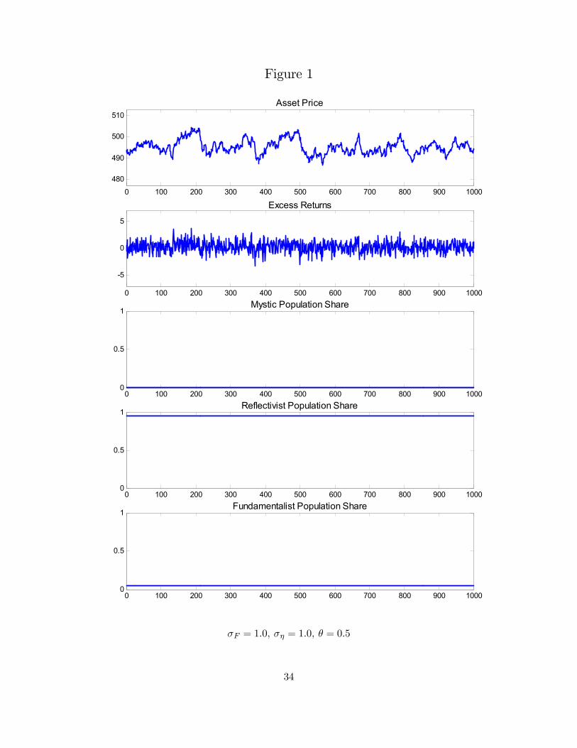
Figure 1

0 100 200 300 400 500 600 700 800 900 1000

480

490

500

510Asset Price

0 100 200 300 400 500 600 700 800 900 1000

-5

0

5

Excess Returns

0 100 200 300 400 500 600 700 800 900 10000

0.5

1Mystic Population Share

0 100 200 300 400 500 600 700 800 900 10000

0.5

1Reflectivist Population Share

0 100 200 300 400 500 600 700 800 900 10000

0.5

1Fundamentalist Population Share

σF = 1.0, ση = 1.0, θ = 0.5

34

Figure 2

0 100 200 300 400 500 600 700 800 900 1000

480

490

500

510Asset Price

0 100 200 300 400 500 600 700 800 900 1000

-5

0

5

Excess Returns

0 100 200 300 400 500 600 700 800 900 10000

0.5

1Mystic Population Share

0 100 200 300 400 500 600 700 800 900 10000

0.5

1 Reflectivist Population Share

0 100 200 300 400 500 600 700 800 900 10000

0.5

1Fundamentalist Population Share

σF = 1.0, ση = 1.0, θ = 1.0

35

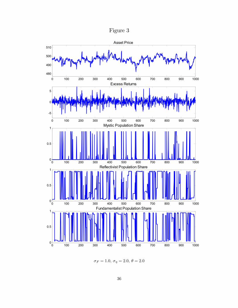
Figure 3

0 100 200 300 400 500 600 700 800 900 1000

480

490

500

510Asset Price

0 100 200 300 400 500 600 700 800 900 1000

-5

0

5

Excess Returns

0 100 200 300 400 500 600 700 800 900 10000

0.5

1Mystic Population Share

0 100 200 300 400 500 600 700 800 900 10000

0.5

1Reflectivist Population Share

0 100 200 300 400 500 600 700 800 900 10000

0.5

1Fundamentalist Population Share

σF = 1.0, ση = 2.0, θ = 2.0

36

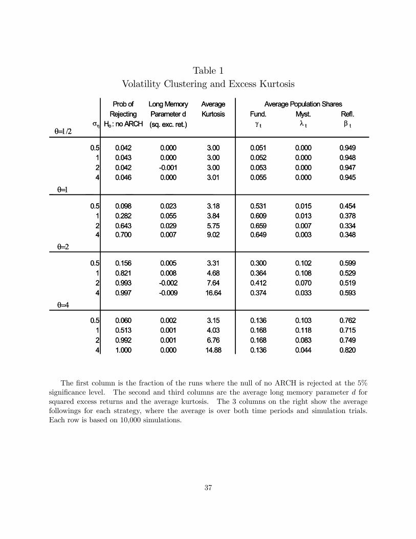
Table 1Volatility Clustering and Excess Kurtosis

Prob of Long Memory Average Average Population SharesRejecting Parameter d Kurtosis Fund. Myst. Refl.

ση Ho : no ARCH (sq. exc. ret.) γ t λ t β t

0.5 0.042 0.000 3.00 0.051 0.000 0.9491 0.043 0.000 3.00 0.052 0.000 0.9482 0.042 -0.001 3.00 0.053 0.000 0.9474 0.046 0.000 3.01 0.055 0.000 0.945

θ=1

0.5 0.098 0.023 3.18 0.531 0.015 0.4541 0.282 0.055 3.84 0.609 0.013 0.3782 0.643 0.029 5.75 0.659 0.007 0.3344 0.700 0.007 9.02 0.649 0.003 0.348

θ=2

0.5 0.156 0.005 3.31 0.300 0.102 0.5991 0.821 0.008 4.68 0.364 0.108 0.5292 0.993 -0.002 7.64 0.412 0.070 0.5194 0.997 -0.009 16.64 0.374 0.033 0.593

θ=4

0.5 0.060 0.002 3.15 0.136 0.103 0.7621 0.513 0.001 4.03 0.168 0.118 0.7152 0.992 0.001 6.76 0.168 0.083 0.7494 1.000 0.000 14.88 0.136 0.044 0.820

θ=1/2

Prob of Long Memory Average Average Population SharesRejecting Parameter d Kurtosis Fund. Myst. Refl.

ση Ho : no ARCH (sq. exc. ret.) γ t λ t β t

0.5 0.042 0.000 3.00 0.051 0.000 0.9491 0.043 0.000 3.00 0.052 0.000 0.9482 0.042 -0.001 3.00 0.053 0.000 0.9474 0.046 0.000 3.01 0.055 0.000 0.945

θ=1

0.5 0.098 0.023 3.18 0.531 0.015 0.4541 0.282 0.055 3.84 0.609 0.013 0.3782 0.643 0.029 5.75 0.659 0.007 0.3344 0.700 0.007 9.02 0.649 0.003 0.348

θ=2

0.5 0.156 0.005 3.31 0.300 0.102 0.5991 0.821 0.008 4.68 0.364 0.108 0.5292 0.993 -0.002 7.64 0.412 0.070 0.5194 0.997 -0.009 16.64 0.374 0.033 0.593

θ=4

0.5 0.060 0.002 3.15 0.136 0.103 0.7621 0.513 0.001 4.03 0.168 0.118 0.7152 0.992 0.001 6.76 0.168 0.083 0.7494 1.000 0.000 14.88 0.136 0.044 0.820

θ=1/2

The first column is the fraction of the runs where the null of no ARCH is rejected at the 5%significance level. The second and third columns are the average long memory parameter d forsquared excess returns and the average kurtosis. The 3 columns on the right show the averagefollowings for each strategy, where the average is over both time periods and simulation trials.Each row is based on 10,000 simulations.

37

Table 2Estimates of GARCH(1,1) Models

Conditional Conditional ConditionalProb of Mean of Prob of Mean of Rejection

Rejecting Estimates Rejecting Estimates Probση Ho : ϕ= 0 of ϕ Ho : ψ= 0 of ψ Q test

0.5 0.150 0.771 0.333 0.044 0.0001 0.087 0.731 0.250 0.048 0.0002 0.139 0.742 0.200 0.041 0.2004 0.182 0.622 0.300 0.067 0.000

θ = 10.5 0.258 0.747 0.708 0.053 0.042

1 0.483 0.760 0.884 0.060 0.0552 0.672 0.642 0.973 0.085 0.0554 0.601 0.509 0.988 0.138 0.059

θ = 20.5 0.348 0.696 0.704 0.064 0.111

1 0.350 0.442 0.997 0.178 0.0802 0.702 0.198 1.000 0.493 0.0394 0.586 0.104 1.000 0.838 0.048

θ = 40.5 0.258 0.822 0.375 0.034 0.000

1 0.193 0.621 0.790 0.087 0.0842 0.222 0.223 0.996 0.390 0.0864 0.281 0.110 1.000 0.859 0.075

θ = 1/2

Conditional Conditional ConditionalProb of Mean of Prob of Mean of Rejection

Rejecting Estimates Rejecting Estimates Probση Ho : ϕ= 0 of ϕ Ho : ψ= 0 of ψ Q test

0.5 0.150 0.771 0.333 0.044 0.0001 0.087 0.731 0.250 0.048 0.0002 0.139 0.742 0.200 0.041 0.2004 0.182 0.622 0.300 0.067 0.000

θ = 10.5 0.258 0.747 0.708 0.053 0.042

1 0.483 0.760 0.884 0.060 0.0552 0.672 0.642 0.973 0.085 0.0554 0.601 0.509 0.988 0.138 0.059

θ = 20.5 0.348 0.696 0.704 0.064 0.111

1 0.350 0.442 0.997 0.178 0.0802 0.702 0.198 1.000 0.493 0.0394 0.586 0.104 1.000 0.838 0.048

θ = 40.5 0.258 0.822 0.375 0.034 0.000

1 0.193 0.621 0.790 0.087 0.0842 0.222 0.223 0.996 0.390 0.0864 0.281 0.110 1.000 0.859 0.075

θ = 1/2

The first column is the fraction of the runs where the GARCH parameter ϕ is significantlypositive, conditional on the presence of ARCH effects. The following column shows the mean ofthe estimates of ϕ for the runs where ARCH effects are present and ϕ is significantly positive. Thenext column shows the fraction of the runs where the ARCH parameter ψ is significantly positive,conditional on ARCH effects being present and ϕ being significantly positive. The following columnshows the mean of the estimates of ψ where ARCH effects are present and ψ and ϕ are significantlypositive. The last column shows the fraction of the runs rejected by the diagnostic Q test amongthose that had ARCH effects and a significantly positive ϕ. Each row is based on 1,000 simulations.

38