an evaluation of the traveling wave ultrasonic motor for force feedback applications
TRANSCRIPT

University of KentuckyUKnowledge
University of Kentucky Master's Theses Graduate School
2009
AN EVALUATION OF THE TRAVELINGWAVE ULTRASONIC MOTOR FOR FORCEFEEDBACK APPLICATIONSNishant VenkatesanUniversity of Kentucky
Click here to let us know how access to this document benefits you.
This Thesis is brought to you for free and open access by the Graduate School at UKnowledge. It has been accepted for inclusion in University ofKentucky Master's Theses by an authorized administrator of UKnowledge. For more information, please contact [email protected].
Recommended CitationVenkatesan, Nishant, "AN EVALUATION OF THE TRAVELING WAVE ULTRASONIC MOTOR FOR FORCE FEEDBACKAPPLICATIONS" (2009). University of Kentucky Master's Theses. 575.https://uknowledge.uky.edu/gradschool_theses/575

ABSTRACT OF THESIS
AN EVALUATION OF THE TRAVELING WAVE ULTRASONIC MOTOR FOR FORCE FEEDBACK APPLICATIONS
The traveling wave ultrasonic motor is considered for use in haptic devices where a certain input-output relation is desired between the applied force and the resulting motion. Historically, DC motors have been the standard choice for this purpose. Owing to its unique characteristics, the ultrasonic motors have been considered an attractive alternative. However, there are some limitations when using the ultrasonic motor for force-feedback applications. In particular, direct torque control is difficult, and the motor can only supply torque in the direction of motion. To accommodate these limitations we developed an indirect control approach. The experimental results demonstrate that the model reference control method was able to approximate a second order spring-damper system. KEYWORDS: Traveling wave ultrasonic motor, haptic device, force-feedback, model reference control method, spring-damper system
Nishant Venkatesan
February 13, 2009

AN EVALUATION OF THE TRAVELING WAVE ULTRASONIC MOTOR FOR FORCE FEEDBACK APPLICATIONS
By
Nishant Venkatesan
Dr. Thomas M. Seigler
Director of Thesis
Dr. L.S.Stephens Director of Graduate Studies
February 13, 2009

RULES FOR THE USE OF THESIS
Unpublished theses submitted for the Masters degree and deposited in the University of
Kentucky Library are as a rule open for inspection, but are to be used only with due
regard to the rights of the authors. Bibliographical references may be noted, but
quotations or summaries of parts may be published only with the permission of the
author, and with the usual scholarly acknowledgments.
Extensive copying or publication of the thesis in whole or in part also requires the
consent of the Dean of the graduate School of the University of Kentucky.
A library that borrows this dissertation for use by its patrons is expected to secure the
signature of each user.
Name
Date
_______________________________________________________________________ _______________________________________________________________________ _______________________________________________________________________ _______________________________________________________________________ _______________________________________________________________________ _______________________________________________________________________ _______________________________________________________________________ _______________________________________________________________________

THESIS
Nishant Venkatesan
The Graduate School
University of Kentucky
2009

AN EVALUATION OF THE TRAVELING WAVE ULTRASONIC MOTOR FOR FORCE FEEDBACK APPLICATIONS
THESIS
A thesis submitted in partial fulfillment of the requirements for the degree of Master of Science
in Mechanical Engineering in the College of Engineering at the University of Kentucky
By
Nishant Venkatesan
Lexington, Kentucky
Director: Dr. Thomas M. Seigler, Professor of
Mechanical Engineering
Lexington, Kentucky
2009
Copyright © Nishant Venkatesan 2009

DEDICATION
To my parents, relatives, and friends

iii
ACKNOWLEDGEMENTS
"A champion is someone who goes so far they can't go another inch—and then they go
that inch." I wondered why that was important. Now I know,winning in business or in
personal life is all about inches: going small distances successfully, then going farther
still.”
I believe we are all born with a purpose and the potential to achieve it. It may take us
years to decide to go for it. When we do, that is the moment we begin our personal road
of trials. We know we are moving closer to our goal when the trials get bigger, and we
see many people around us giving up – we keep going, over the last massive trial and
achieve our pot of gold.
A BIG thanks to you, Dr. Seigler for giving me an opportunity to be part of your team,
share your ideas, pick up threads from your wisdom, constantly upgrade my knowledge
and above all bearing with me and relentlessly encouraging me whenever I erred. For
every life there must be a path breaker and you have proved to be one for my success. By
your presence, by your example, by your action and inaction, by your words and deeds,
by your blessings and support, by your understanding and love, today I stand in front of
you as a ‘MAN’ with a sense of accomplishment and achievement. Yes, I do remember
your words that education is a progressive discovery of our own ignorance and in this
world there is no real achievement till we retire and leave a legacy that the humanity
would recognize and remember for years to come by.
My thanks to my mother and father, Revathi and Venkatesan, Jayshri, Ramakrishnan, my
brother Thejaswin and to a very special person, Varsha Kumar who contributed to this
effort, and kept me going with their belief, support and inspiration when it was most
needed. I extend my heart full greetings to my friends from India, specially Dr.
Anantharaman Muthuswamy and Dr. Padhma Ranganathan who have been with me all
through my turmoil, downs, ill health, slips, and sleepless nights. Never did they exhibit
their anguish or anxiety that made my journey smoother and pleasanter.

iv
TABLE OF CONTENTS
ACKNOWLEDGEMENTS ........................................................................................................................... iii
LIST OF TABLES ......................................................................................................................................... vi
LIST OF FIGURES ....................................................................................................................................... vii
1 Introduction............................................................................................................................................ 1
1.1 MOTIVATION ..................................................................................................................................... 1
1.2 OBJECTIVES ....................................................................................................................................... 2
1.3 OUTLINE ............................................................................................................................................ 2
1.4 CONTRIBUTIONS ................................................................................................................................ 3
2 Background ........................................................................................................................................... 4
2.1 OPERATING PRINCIPLES ..................................................................................................................... 4
2.1.1 The Traveling Wave Ultrasonic Motor .................................................................................... 6
2.2 MATHEMATICAL MODELS OF THE USM ............................................................................................ 9
2.2.1 Equivalent Electrical Model .................................................................................................. 10
2.2.2 Equivalent mechanical model ................................................................................................ 11
2.3 CONTACT MECHANICS ..................................................................................................................... 13
2.4 CONTROLS RESEARCH ..................................................................................................................... 15
2.5 SUMMARY........................................................................................................................................ 16
3 Experimental Setup .............................................................................................................................. 17
3.1 INSTRUMENTATION ......................................................................................................................... 18
3.1.1 USR 60 Shensei...................................................................................................................... 19
3.1.2 AG 1006 amplifier ................................................................................................................. 20
3.1.3 Torque transducer ................................................................................................................. 20
3.1.4 Mechanical brake .................................................................................................................. 20
3.1.5 DC motor ............................................................................................................................... 21
3.2 DATA ACQUISITION ........................................................................................................................ 23
4 Force Feedback Control ....................................................................................................................... 25
4.1 FORCE FEEDBACK OPERATION ........................................................................................................ 25
4.2 FORCE FEEDBACK CONTROL APPROACH ........................................................................................ 28
4.3 STEADY STATE PROPERTIES ............................................................................................................ 30

v
4.3.1 Effects of frequency modulation ............................................................................................ 31
4.3.2 Torque Speed Characteristics for Various Frequencies ........................................................ 32
4.3.3 Effects of phase modulation ................................................................................................... 33
4.4 CONTROL FORMULATION ................................................................................................................ 37
4.4.1 Frequency Control ................................................................................................................. 37
4.4.2 Phase Control ........................................................................................................................ 38
4.5 SUMMARY ....................................................................................................................................... 38
5 Experimental Evaluations .................................................................................................................... 39
5.1 POSITION REFERENCE TRACKING.................................................................................................... 39
5.1.1 Frequency Control ................................................................................................................. 40
5.1.2 Phase Control ........................................................................................................................ 48
5.2 FORCE FEEDBACK ........................................................................................................................... 54
5.2.1 Force Feedback-Pulse Input ................................................................................................. 55
5.2.2 Force Feedback for Sinusoidal Inputs ........................................................................................ 60
6 Conclusions and Future Work ............................................................................................................. 68
6.1 CONCLUSION ................................................................................................................................... 68
6.2 FUTURE WORK ................................................................................................................................ 69
APPENDIX A ............................................................................................................................................... 70
APPENDIX B ............................................................................................................................................. 106
References ................................................................................................................................................... 108
Vita .............................................................................................................................................................. 113

vi
LIST OF TABLES
Table 3.1. Specifications of USR 60 ..............................................................................................19
Table 3.2. Specifications of DC Motor ..........................................................................................21
Table 3.3. Specifications of Incremental encoder ..........................................................................22

vii
LIST OF FIGURES
Figure 2-1. Basic Construction of Ultrasonic Motor [1] ..................................................................4
Figure 2-2. Classifications of Ultrasonic Motors .............................................................................5
Figure 2-3. Disc Type Stator ............................................................................................................6
Figure 2-4 (a) and (b). Piezoelectric actuation of the traveling wave ultrasonic motor: actuation
concept and 2-4 (b) actuator arrangement for a 4-λ stator. ..............................................................8
Figure 2-5. Traveling Wave Ultrasonic Motor USR 60 [42] ...........................................................9
Figure 2-6. Stator model of TWUSM ............................................................................................10
Figure 2-7. Simplified equivalent circuit of the USM [4] .............................................................11
Figure 2-8. Equivalent Mechanical Circuit-Single input [17] .......................................................12
Figure 2-9. Equivalent Mechanical Model [17] .............................................................................13
Figure 2-10. Stator-rotor Contact Model .......................................................................................14
Figure 3-1. Test bench set up for determining the Speed Torque Characteristics .........................17
Figure 3-2. Experimental Setup .....................................................................................................18
Figure 3-3. Mechanical Brake Provided for Applying Resistive Torque ......................................21
Figure 3-4. Simulink Block Diagram .............................................................................................24
Figure 4-1. Comparison of the torque transmission for a DC motor and an ultrasonic motor: (a)
the torque supplied by a DC motor is primarily dependent on the current; (b) torque transmission
for the ultrasonic motor is based upon contact friction. .................................................................26
Figure 4-2. Force-feedback approach; input disturbance based position control ..........................29
Figure 4-3. Speed Vs Frequency ....................................................................................................32
Figure 4-4. Speed Vs Torque curves for various frequencies ........................................................33
Figure 4-5.Speed Vs Phase for various Torque .............................................................................34
Figure 4-6.Speed Vs Torque curves for a phase range at 40.5K Hz ..............................................35
Figure 4-7.Speed Vs Torque curves for a phase range at 41K Hz .................................................36
Figure 4-8. Speed Vs Torque curves for a phase range at 41.5K Hz .............................................36
Figure 5-1. Constant Reference Tracking ......................................................................................39
Figure 5-2. Effects of upper frequency (fmax) on steady-state tracking performance .....................41

viii
Figure 5-3. Effects of proportional gain on constant reference tracking frequency control; r(t) =
10°. .................................................................................................................................................42
Figure 5-4. Commanded excitation frequency corresponding to Figure5-3 ....................42
Figure 5-5. Effects of integral gain on constant reference tracking frequency control; r(t) = 10° 43
Figure 5-6. Commanded excitation frequency corresponding to Figure5-5. .................................43
Figure 5-7. Effects of derivative gain on constant reference tracking frequency control; r(t) = 10° 44
Figure 5-8. Commanded excitation frequency corresponding to Figure5-7 ..................................44
Figure 5-9. Effects of proportional gain on model reference tracking frequency control .............45
Figure 5-10. Commanded excitation frequency corresponding to .................................................46
Figure 5-11. Effects of integral gain on model reference tracking frequency control ...................46
Figure 5-12.Commanded excitation frequency corresponding to Figure ......................................47
Figure 5-13. Experimental closed-loop frequency response of position reference tracking. ........48
Figure 5-14. Effects of proportional gain on constant reference tracking phase control. ..............49
Figure 5-15. Commanded excitation phase corresponding to Figure5-14 .....................................50
Figure 5-16. Effects of integral gain on constant reference tracking phase control. .....................51
Figure 5-17. Commanded excitation phase corresponding to Figure5-16 .....................................51
Figure 5-18. Effects of proportional gain on model reference tracking frequency control ...........52
Figure 5-19. Excitation phase corresponding to Figure 5-18 ........................................................53
Figure 5-20. Effects of integral gain on model reference tracking frequency control. ..................53
Figure 5-21. Excitation phase corresponding to Figure 5-20 ........................................................54
Figure 5-22. Position tracking for varying torque-2Hz user input .................................................56
Figure 5-23. Commanded excitation frequency corresponding to Figure 5-22 .............................56
Figure 5-24. Position tracking for varying torque-3Hz .................................................................57
Figure 5-25. Commanded excitation frequency corresponding to Figure 5-24 .............................57
Figure 5-26. Position tracking for varying torque-2Hz user input .................................................58
Figure 5-27. Commanded excitation phase corresponding to Figure 5-26 ....................................59
Figure 5-28. Position tracking for varying torque-3Hz user input .................................................59
Figure 5-29. Commanded excitation phase corresponding to Figure 5-28 ....................................60
Figure 5-30. Position tracking for varying torque-1 Hz user input ................................................61
Figure 5-31. Commanded excitation frequency corresponding to Figure 5-30 .............................61

ix
Figure 5-32. Position tracking for varying torque-1Hz user input .................................................62
Figure 5-33.Commanded excitation frequency corresponding to Figure 5-32 ..............................62
Figure 5-34. Closed-loop frequency response Θ(iω)/TL(iω) for reference model parameters ωn =
4π rad/s and ζ = 0.1. .......................................................................................................................63
Figure 5-35. Closed-loop frequency response Θ(iω)/TL(iω) for reference model parameters ωn =
4π rad/s and ζ = 0.5 ........................................................................................................................64
Figure 5-36. Position tracking for varying torque-1Hz user input .................................................65
Figure 5-37. Commanded excitation phase corresponding to Figure 5-36 ....................................66
Figure 5-38. Position tracking for varying torque-2 Hz user input ................................................66
Figure 5-39. Commanded excitation phase corresponding to Figure 5-38 ....................................67

1
1 Introduction
The purpose of this research is to evaluate the traveling wave type ultrasonic motor for use in
devices that require force feedback. A general overview of the thesis work, including motivation,
objectives and outlines are laid out in this chapter.
1.1 Motivation
The traveling wave ultrasonic motor (USM), hereafter referred to as simply USM, is considered
for use in haptic devices where feedback forces are required, in particular force-feel systems
where a certain input-output relation is desired between the applied torque and the response.
Owing to some of its unique characteristics, there are circumstances where the ultrasonic motor
may be considered an attractive alternative to the more standard electromagnetic motor. In
particular:
1. The USM is a low speed high torque device. To achieve this with the electromagnetic
motor requires gearing which can add dynamic complexity.
2. The ultrasonic motor has a torque density in the range three to ten times higher than a DC
motor.
3. USM neither generates nor is affected by an electromagnetic field.
4. The motor has a high holding torque in the absence of input energy, where as the
electromagnetic motor requires both electrical energy and feedback control to hold a
desired position under load.
However, the USM and electromagnetic motor are significantly different in their operating
principles and are not necessarily interchangeable in all applications. The USM can only output
torque in the direction of the rotation. The electromagnetic motor is not so constrained.
Additionally, the output torque of the USM is difficult to directly control. In contrast, for the DC
motor the output torque is simply controlled by current. Hence, to be considered a viable
alternative in force-feedback applications, we seek an approach to torque control for the USM.

2
1.2 Objectives
The primary objective of this research is to develop a control method for the USM that can be
used in force feedback applications; and to experimentally evaluate its performance. This
objective was achieved by the following tasks.
1. Experiment development, which includes arranging a closed loop experimental setup and
evaluating the steady state performance.
2. Control development, which includes formulating the control algorithms, based on the
steady state characteristics of the USM.
3. Experimental validation of the control method, which includes the evaluation of the USM
in force feedback operation.
Evaluation was based on the ability to generate a desired input-output response between the user
input and the output motion.
1.3 Outline
This thesis is divided into six chapters, the contents of which are as follows.
Chapter 2 contains a literature review, which discusses in detail the construction and working
principle of USM. A survey of various mathematical models is presented, the purpose of which
is to analyze the relationship between the input parameters and the output torque, which is
normally required for force-feedback control.
Chapter 3 contains a detailed description of the experimental setup. Specifications of the major
components and data acquisition methods are discussed.
Chapter 4 introduces the force-feedback control approach that is considered in this work.
Experimental results are provided to demonstrate the basic functionality of the motor.
Chapter 5 presents an experimental validation of the USM force-feedback control methodology.

3
Chapter 6 contains the conclusion of the research and suggestions for future work.
The Appendix contains supplementary experimental results, not crucial to the main contents of
the work.
1.4 Contributions
As mentioned, controlling the torque of the USM is a difficult task. Previous researches have
developed complex approaches that have mostly relied on steady state operating characteristics.
However, none of these works has considered an arbitrary time varying load that occurs in force-
feedback applications. Nor, in their control formulations have they considered the basic
limitation that the USM can supply torque only in the direction of motion. To accommodate
these limitations we have developed a model reference force-feedback control method.
Experimental results demonstrate that the closed-loop system is able to approximate a simple
second-order response, thus producing the feel of a spring and damper.

4
2 Background
This chapter presents a brief summary of the working principle, historical background, and the
various mathematical models of the traveling wave ultrasonic motor. The basic operating
principles of the USM are examined to explain the basic limitations. Keeping in mind that the
focus of investigation is force-feedback application, various mathematical models are surveyed
for their usefulness in predicting the torque produced by the USM.
2.1 Operating Principles
The ultrasonic motor is a type of piezoelectric actuator that consists of three basic parts: a
piezoelectric actuator, an elastic vibrator, and a sliding piece, as shown in Figure 2-1[1]. The
piezoelectric actuator is attached to the elastic vibrator. The friction coat along with the elastic
moving part constitutes the sliding piece. A high frequency input signal, in the ultrasonic range
(> 20kHz), is supplied to the actuator to excite the elastic vibrator at high amplitude. The
vibration of surface points of the elastic vibrator is transmitted through contact friction and
generates motion of the sliding piece.
Figure 2-1. Basic Construction of Ultrasonic Motor [1]
High frequency input
Electrical Input
Piezoelectric Actuator Elastic Vibrator
Friction Coat Elastic Sliding Piece

5
There are various types of ultrasonic motors. As shown in Figure 2-2, they are broadly classified
into standing wave type and traveling wave type [1, 2, 3]. Standing wave ultrasonic motor use the
standing wave generated in the elastic vibrator to drive the sliding piece. The direction of motion
of the particles on the standing wave depends on the position of the particle. The traveling wave
USM uses the traveling wave generated in the elastic vibrator to drive the sliding piece.
Figure 2-2. Classifications of Ultrasonic Motors
Though the first standing wave ultrasonic motor was invented in 1965 by V.V. Lavrinenko, the
first practical ultrasonic motor, proposed by H.V Barth of IBM came into existence in 1973.
Various mechanisms based on the same principle were proposed by Lavrinenko and Vasilev in
the former USSR [1, 4]. The traveling wave ultrasonic motor was invented by T.Sashida in 1982.
The following section details the traveling wave ultrasonic motor, since this is the focus of the
current work.
Ultrasonic Motors
Standing Wave Traveling Wave
Bidirectional Unidirectional
Systems with two or more
actuators Single Actuator System

6
2.1.1 The Traveling Wave Ultrasonic Motor
The traveling wave ultrasonic motor (USM) is designed on the basic principle that by actuating
transverse traveling wave motion of an elastic medium, the surface points of that medium
produce an elliptical trajectory that can be used to transfer energy to a contacting surface.
Referring to Figure 2-1, for the USM, the elastic vibrator in conjunction with the piezoelectric
actuator constitutes the stator. For an elastic medium of arbitrary geometry, the generation of a
traveling wave is not trivial; however thin circular disks and shells are amenable to this type of
motion. The transverse free vibration solution, (i.e. mean plane solution) of a thin disk ( Figure
2-3), is , where B(r) is a dimensionless Bessel’s function, r and φ
are the spherical coordinates, and ω is the angular frequency.
Figure 2-3. Disc Type Stator
For a disk, the defined origin for measurement of angular displacement is arbitrary, hence
B(r)sinmφ sinωt is also another vibration solution for the disk. Both the solutions represent
standing waves. A traveling wave is obtained by the superposition of these standing waves, that
is
)cos()(sinsin)(coscos)( tmrBtmrBtmrB ωφωφωφ −=+ (2.1)
tmrBtrw ωϕϕ coscos)(),,( =
ϕ
r
R h
z

7
For r=R, the outer radius of the disk, the surface motion of the disk is written as )cos( φω −tA .
The surface motion is calculated by Euler’s hypothesis, which assumes that the mean plane
sections remain plane during deformation. It can be shown that the motion of the surface points
on the stator is an elliptical trajectory [5], of the form
)()],,,([)],,,([ 2222 rRAtzrwhmrtzrwz =+ φφ φ (2.2)
where, wz and wφ are vibration amplitudes in z and φ directions. The velocity of the points on the
peak of the ellipse is found by differentiating Equation 2.2 with respect to time [3, 5, 6, 7, 8]:
(2.3)
where h is the mean plane thickness, and λ is the wave length. Note from Equation 2.3 that the
velocity of the particles on the surface increases with increase in frequency, thickness and
vibration amplitude. However, increasing the vibration amplitude or the stator thickness requires
larger actuation energy. Also, Equation 2.3 seems to imply that the velocity of surface points is
proportional to frequency. However, the amplitude A is a function of frequency. In particular, the
amplitude decreases with an increase in frequency; hence the velocity is not proportional to
frequency.
The construction principle for the USM is shown in the Figure 2-4 (a). Ceramics with opposite
polarization are placed consecutively so that one will expand while the other will contract when
a voltage is supplied. The expansion and contraction of the ceramics causes a transverse
traveling wave on the mean plane of the elastic body, which produces elliptical motion of the
surface points. Two input signals Acos(2πft) and Asin(2πft+φ) are supplied to the actuator. Thus,
the control parameters are the input frequency, amplitude and phase. A physical arrangement of
piezoelectric ceramics is shown in the Figure 2-4 (b) for a mode-4 actuation scheme.
λπωhAvs =

8
Figure 2-4 (a) and (b). Piezoelectric actuation of the traveling wave ultrasonic motor:
actuation concept and 2-4 (b) actuator arrangement for a 4-λ stator.
A cut-away section indicating the parts of the motor is shown in the Figure 2-5, which includes
the piezoelectric ceramic, the stator, the rotor, the bearings, and the case. Another part which
requires special mention is the comb teeth. They are the grooves that appear between the stator
and the rotor. To explain these comb teeth, note from Equation 2.3 that the velocity of the
surface points is proportional to mid plane thickness of the stator; hence the velocity can be
effectively increased by increasing the thickness of the stator, which is achieved by adding comb
teeth. The teeth helps to increase the thickness of the stator without substantially changing the
natural frequency. The gaps between the teeth also help in removing the dust produced due to
friction.
piezoelectric ceramic
contractionexpansion
expansioncontraction
(a) (b)
electrode
surface

9
Figure 2-5. Traveling Wave Ultrasonic Motor USR 60 [42]
2.2 Mathematical Models of the USM
Due to the complexity in the working principle, the motor’s physical behavior is difficult to
model. Determination of the output torque of the USM is highly complex because it is dependent
not only on the surface motion of the stator but also on the interaction between the stator and the
rotor. In contrast, a model of the DC motor, which is the actuator most often used for force-
feedback applications, is relatively simple. There exists an approximate linear relationship
between the input current and the output torque.
Over the past several years, researchers have been working toward the development of
mathematical models for the USM that can be used to predict the relationship between the input
excitation parameters and output parameters such as speed and torque. The following discussion
provides an overview of the various mathematical models that have been suggested in the
literature.

10
2.2.1 Equivalent Electrical Model
The theory of electrical circuits is often useful in resolving the complex dynamic or static
behavior of mechanical systems. Electrical equivalent components such as capacitors, inductors,
and resistors have been used for modeling components of the USM. Such a model for the USM
stator is shown in Figure 2-6. The first stage constitutes the voltage supply to the ceramic, which
is indicated by the AC supply to the piezoelectric ceramic. Actuation of the two modes is
possible by supplying the voltages with a phase difference. An equivalent capacitance, Cd,
represents the piezoelectric ceramic. The stator’s mass is equivalent to the inductor Lm, its
capacitance is given by Cm, and an overall loss is modeled by a resistor denoted by ro. The two
loops represent the two out of phase vibration solutions of the stator. In this model, it is assumed
that there is no cross coupling, in that the two vibration modes do not affect one another.
Figure 2-6. Stator model of TWUSM
Figure 2-7 represents an electrical equivalent model of the entire USM [4, 9, 10, 11, 12, 13, 14,
15, 16] for the case where the two input excitation signals are 90˚ out of phase. The rotor is
considered to be a rigid body of mass Lm. Ideally, there are no frictional losses in converting the
vibration of the stator into motion of the rotor. However, in reality some amount of heat is
generated due to the sliding between the stator and the rotor. This is considered frictional loss,
AC
Cd
CmLm
ro
AC
Phase A
Phase B
Cd

11
which is represented by a diode and a resistor connected in parallel to a transformer. The
vibration during the actuation of the motor, mechanical losses and viscous losses in the bearings
and other related parts of the USM determines the total losses in the motor which is given by rL.
The transformer between the stator and the rotor provides the simplest possible description of the
contact mechanics.
Figure 2-7. Simplified equivalent circuit of the USM [4]
From Figure 2-7, the two circuits represent the out-of-phase vibration solution of the stator,
while the output obtained is the current across the diode, which is representative of the motor
speed. We note that this equivalent circuit model cannot be used to predict the torque of the
motor and is thus of little use for force-feedback applications.
2.2.2 Equivalent mechanical model
One modeling approach, which builds upon the equivalent electrical model of the USM to
encompass more details such as the cross coupling between modes, was suggested by Kandare et
al. [16, 17]. This approach we refer to as the equivalent mechanical model. Mechanical
equivalents such as mass, spring and dampers are used to develop the equivalent mechanical
model. Resistor RP, represents losses in the piezo-ceramics and the capacitor CP represents its
capacitance. The transformer with a ratio A, represents the electromechanical coupling between
the electrical and the mechanical system.
Va
1:n
Lm cm ro
Lm
DL
rL
cmro
Vb
Lm

12
Figure 2-8. Equivalent Mechanical Circuit-Single input [17]
The model shown in Figure 2-8 is identical to the equivalent electrical model shown in Figure 2-
7. Here the symmetrical disturbances are not taken into consideration, which makes the model an
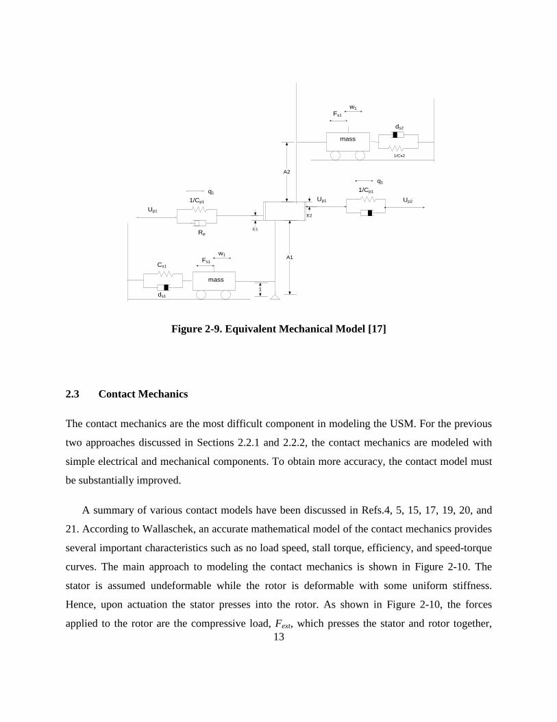
ideal one [18]. To account for cross coupling between the vibration modes, symmetrical
disturbances, indicated by E1 and E2 in Figure 2-9, are added [16]. As with the equivalent circuit
model, the purpose of this model is to output the speed of the motor as a function of excitation
parameters. However, in this model, in addition to amplitude and frequency, the excitation phase
can also be considered.
A
1
Up
q
1/Cp
Rp
wFs
ds
Cs
mass
13
Figure 2-9. Equivalent Mechanical Model [17]
2.3 Contact Mechanics
The contact mechanics are the most difficult component in modeling the USM. For the previous
two approaches discussed in Sections 2.2.1 and 2.2.2, the contact mechanics are modeled with
simple electrical and mechanical components. To obtain more accuracy, the contact model must
be substantially improved.
A summary of various contact models have been discussed in Refs.4, 5, 15, 17, 19, 20, and
21. According to Wallaschek, an accurate mathematical model of the contact mechanics provides
several important characteristics such as no load speed, stall torque, efficiency, and speed-torque
curves. The main approach to modeling the contact mechanics is shown in Figure 2-10. The
stator is assumed undeformable while the rotor is deformable with some uniform stiffness.
Hence, upon actuation the stator presses into the rotor. As shown in Figure 2-10, the forces
applied to the rotor are the compressive load, Fext, which presses the stator and rotor together,
A1
1
q1
Up1
1/Cp1
Rp
q1
Up1
1/Cp1
w1Fs1
ds1
Cs1
mass
mass
ds2
1/Cs2
w1Fs1
Up2
A2
E1
E2

14
and the stator-rotor interaction forces, FN and FT, the normal and tangential force, respectively.
The forces applied to the stator are provided by the piezoelectric actuating elements and the
stator-rotor interaction. Here we have a fundamental difficulty in modeling the dynamics of this
system (as with all systems that involve contact mechanics): the interaction forces acting
between the stator and rotor are dependent on the motion of the stator and rotor. That is, in order
to even define the interaction forces, the motion must be known; knowing the motion amounts to
solving equations of motion, for which the forces must be specified. The contact mechanics
problem can be resolved to some degree by numerical simulation, where time delays can be
imposed. However, this is not very useful for analytical evaluation, and in particular for control
design where, ideally, the torque is expressed as a function of the piezo ceramic inputs (voltage
amplitude, excitation frequency and phase). Moreover, the equations of motion that have been
developed for the USM, through consideration of the contact mechanics, are highly nonlinear.
The torque is related to the input parameters (voltage amplitude, frequency, and phase) through
several coupled nonlinear ordinary differential equations, and transcendental algebraic equations.
Even steady-state analytical solutions are, to our knowledge, not possible for these equations.
This poses a severe difficulty in attempting to design a model-based compensator to control the
torque. As discussed in Chapter 4, we will circumvent this difficulty with a model reference
based control approach.
Figure 2-10. Stator-rotor Contact Model
FNR
Rotor
Contact layer
Stator
FTR FN
FT
Fext

15
2.4 Controls Research
Various control techniques have been developed for the USM. We divide these techniques into
speed and position control, and torque control. As mentioned in Section 2.1.1, the input
parameters than can be used to control the motor’s output parameters are frequency, phase and
amplitude of applied voltage. Most control techniques in the literature have utilized only
frequency and phase. Effects of varying amplitudes on the motor’s performance is not examined
because it does not have the ability to control the motor at low speeds and the range of amplitude
in which the motor must operate to achieve high speeds is large.
Speed control based on frequency modulation was demonstrated in Refs. 22 and 23, and a phase
modulation technique was shown in Ref. 24. Arguing that frequency modulation is best suited
for quick response, and phase modulation provides precise positioning, a method called dual
mode control, which combines both frequency and phase modulation simultaneously, was
demonstrated to achieve quick response and precise positioning [25, 26]. To account for time
varying parameters an adaptive control technique was developed [27]. Due to continuous
interaction between the stator and the rotor, there might be wear in the friction coat, which
affects the performance characteristics of the USM. The heat generated during the motor’s
operation also affects its performance. The adaptive control techniques developed accounts for
these losses. In this work, the motor model was assumed to be linear. To accommodate
nonlinearities such as dead-zone effects and hysteresis (discussed later in Chapter 4), controllers
based on fuzzy logic and neural networks were developed [28, 29, 30, 31, 32]. In Ref. 28, the
model reference adaptive control was used to perform precise positioning, while the fuzzy-logic
controller was used to compensate for dead-zone effects.
As discussed in the previous section, torque control of the USM is not straight-forward. Previous
approaches to control torque typically have employed an inverse plant model based on steady
state torque-speed data [33, 34]. Giraud et. al. developed model based control for precise
positioning [35], while J.Maas et.al. developed a model based speed control technique [24].
These works, however, do not consider an arbitrarily time varying load, which occurs in force-

16
feedback applications. Also not taken into account is the inability of the motor to generate torque
in the opposite direction of motion. In force-feedback applications, these limitations do not allow
the motor to produce an arbitrarily specified torque. For example, as detailed in Chapter 4, the
USM cannot be expected to mimic a simple spring damper system
2.5 Summary
The unique characteristics of the USM make it attractive for use in many applications. However,
the operating principles are significantly different than more commonly used electromagnetic
motors, and cannot provide the same functionality in all applications. For example, we cannot
expect the ultrasonic motor to produce the interaction torque that would be provided by a spring-
damper system. Additionally, the models necessary for accurately describing the motion and
torque produced by the ultrasonic motor are complex. Thus, model based control is not straight-
forward. Researchers have been forced to rely on substantial simplifications and learning
algorithms to accommodate model-based control for force feedback operation. Further, the
control approaches that have previously been developed are not applicable to the current study,
which requires that the USM interact with an arbitrarily, and unknown, time-varying load.

17
3 Experimental Setup
The basic experimental setup for our investigation is shown in Figure 3-1. The USM used in
these experiments (Shinsei USR60) requires two input signals at amplitudes of 130 V and at
frequencies in the range of 40 KHz. The sinusoidal waveforms are provided by a DSpace control
board. Two high-voltage amplifiers are used to gain outputs from the DSpace source to the
USM. The torque transducer is coupled to the USM to measure the interaction torque between
the USM and the DC motor. The purpose of the DC motor is to provide positive torque for
torque-speed measurements, and also to act as the human input load for force-feedback
experiments. Negative torques for torque-speed measurements are provided by a mechanical
brake. An incremental position encoder measures the angular position of the motor, which is fed
back to the DSpace control board where it is numerically differentiated to obtain the angular
velocity. Feedback of the torque and the position measurements are later used for active control.
Figure 3-1. Test bench set up for determining the Speed Torque Characteristics
Amplifier 2
Amplifier 1
Cos input USR 60
Sin input Torque
Transducer Position Encoder
Angle Speed
DC Motor DSpace
Torque (N-m)
Mechanical Brake
Matlab/Simulink

18
The actual experimental setup is shown in Figure 3-2. A more detailed description of the
components of this experimental setup is provided in Section 3.1. Data acquisition methods used
in this study detailed in Section 3.2.
Figure 3-2. Experimental Setup
3.1 Instrumentation
The DSpace control board used for the current work contains 16 input and 8 output channels. Of
the 16 input channels 2 input channels are used to supply the excitation signals to the USM. The
operating voltage range for the I/O channels is ± 10V. The channels have an operating frequency
range of 133 MHz at 16 bit resolution. The following subsections detail the specifications of
other components that are used in the experimental setup.
Shensei USR 60 T20WN DC Motor
Brake Incremental encoder

19
3.1.1 USR 60 Shensei
All experimental testing was conducted with the Shensei USR60 ultrasonic motor. The operating
characteristics of the USR 60 are given in the Table 3.1[37]. Note that the response time of the
motor is 0.001 seconds. By the response time, it is meant the time taken for the rotational speed
of the motor to reach steady state given a step input of the excitation parameters (amplitude,
frequency, and phase). This response time is relatively fast compared to dynamics in typical
human interface force-feedback applications; human’s motion is typically confined to the range
of 0 – 5Hz. The response time is thus an important feature, since we can ignore the transient
response of the motor, and focus on steady-state response. This will be an important assumption
in the control development of Chapter 4.
Table 3.1. Specifications of USR 60
Driving Frequency 50 KHz Driving Voltage 120 V Rated Torque 0.5 N-m(5 KgF-cm) Rated Power 5.0W Rotational Speed 100 rpm Maximum Torque 1 N-m or above Holding Torque 1-N-m or above Response Time 1 m sec or below Rotational Direction CW,CCW Lifetime 1000 Hrs Operating Temperature Range -10ºC to 50ºC Operating Temperature Range 55ºC Mass 260 g

20
3.1.2 AG 1006 amplifier
Two T&C Power Conversion AG 1006 high-voltage amplifiers are used to amplify the DSpace
source. The amplifier is a source of RF power used for ultrasonic, industrial, laser modulation
and plasma generation. It can supply up to 300 Watts of power with the frequency ranging
between 20 KHz to 4 MHz. Note that it is possible to use a single amplifier to provide two
signals exactly 90° out of phase. This can be done by integration. In Chapter 4 and 5 we will
consider phase control, where the phase must be varied real-time. Performing this task with a
single amplifier becomes more difficult in this case. Hence, two amplifiers are used in the test so
that an independent sine and a cosine signal can be supplied. Specifications for the amplifier are
provided in Ref. 38.
3.1.3 Torque transducer
The shaft of the motor is coupled to the torque transducer, T20WN, which measures the
interaction torque between the user input provided by the DC motor and the USM. The nominal
torque rating of the transducer used is 5 N-m. The nominal sensitivity is 2V/N-m. The T20WN
has an accuracy class of 0.2, which means that the signal range could be 10 V±0.2% (of the
nominal sensitivity). Some of the special features of the transducer are contactless transmission
of measurement signal, measurement on rotating and stationary parts, integrated measuring
system for speed and angle.
3.1.4 Mechanical brake
A mechanical brake is mounted on the shaft of the transducer that is coupled to the DC motor.
The brake was made of Nylon in order reduce wear to the shaft of the transducer. By tightening
or loosening the brake the torque is increased or decreased, respectively. Figure 3-3 shows a
picture of the mechanical brake used in the experiment.

21
Figure 3-3. Mechanical Brake Provided for Applying Resistive Torque
3.1.5 DC motor
The other end of the torque transducer shaft is coupled to a brush-type DC servo motor
(Aerotech 1000 DC) which applies an input force to the USM. The continuous torque ranges
from 0.25 N-m to 1.48 N-m and the peak torque ranges from 1.84 N-m to 7.1 N-m. The
specifications of the motor are provided in Table 3.2.
Table 3.2. Specifications of DC Motor
Model number 1000 DC
Motor KT 4.1 oz-in/amp
Continuous Torque 17 oz-in
Peak Torque 130 oz-in
Tachometer Kg 3V/KRPM

22
3.1.6 Rotary Incremental Encoder
The shaft on the other end of the DC motor is coupled to a rotary incremental encoder which
generates two data signals that are electrically 90º out of phase [39]. Three signals are given by
the encoder, A, B and index, where A gives the position when the encoder shaft moves in
clockwise direction, while B gives the signal when it moves in counter clockwise direction. The
index signal is given by the respective pins mentioned in Ref. 39. A few of the specifications of
Model 8225 are given in Table 3.3 [39].
Table 3.3. Specifications of Incremental encoder
line count on disc 6,000
cycles/rev with internal electronics 48,000
counts/rev (after quad edge detection) 192,000
cycles/rev with external electronics 120,000
Instrument error 20 arcsec
±

23
3.2 Data Acquisition
All control simulations were conducted in Matlab Simulink and all data were recorded by
DSpace. The basic Simulink block diagram framework is shown in Figure 3-4. This Simulink
code is used to experimentally evaluate the steady state characteristics of the motor (Chapter 4),
and is later updated for control experiments (Chapter 5). The baseline simulation frequency is set
to 160kHz, four times the vibration natural frequency of the USM. Two input signals with a
phase shift are supplied to the amplifiers through two DAC channels with a gain (labeled as
gain). Each of these signals must be amplified to 130 V before provided to the USM. This
amplification is performed by adjusting the gains manually on the T&C amplifiers. By adjusting
the gains on the T&C amplifier it is difficult to obtain two voltage signals exactly equal to 130V.
By adjusting the gain values in Simulink, minor tuning of the signals can be performed to obtain
two voltage signals exactly equal to 130 V. A change in the rotational direction of the motor is
induced by the switches (labeled Direction Change Switches in Figure 3-4). For a positive value
the motor rotates in the forward direction, and for a negative value the motor rotates in the
reverse direction. The saturation block (labeled Saturation in Figure 3-4) maintains the
frequency within specified operating limits; this feature is required for feedback control using
frequency modulation. The atomic subsystem shown in Figure 3-4, is used to sample the angular
position and the change in angular position, interaction torque, and load torque supplied by DC
motor. The measurements made within the subsystem are later used as feedback signals to
perform control. The sample frequency of the atomic subsystem is 1000 Hz.

24
Figure 3-4. Simulink Block Diagram
USM
Inpu
ts
Dire
ctio
n C
hang
e
Switc
hes
gain
Ato
mic
Sub
syst
em
Satu
ratio
n

25
4 Force Feedback Control
The application considered for the USM is a torque source for haptic systems. Generally, a
haptic system is a device that simulates stiffness, weight and inertia [40]. These devices are
important in virtual reality simulations, teleoperation, and various “by-wire” systems.
Historically, brushless DC motors have been the standard choice for providing force feedback in
haptic systems. Due to the unique features mentioned in Chapter 1, the USM may be an
attractive alternative in some applications that require higher energy density, low-speed high-
torque operation, or those where a magnetic field is intolerable. However, as briefly discussed in
Chapter 2, the operating principle of the DC motor is significantly different from the USM. In
this chapter we discuss the major differences more thoroughly, with specific regard to force-
feedback operation. The major contribution of the work is also contained in this chapter, namely
a method of control that can be applied to the USM in force-feedback operation. Because the
response time of the motor is fast relative to the human motor action, the control formulation
relies on basic steady-state behavior as observed in experiments.
4.1 Force Feedback Operation
The primary difference between the DC motor and the USM is the type of force involved. The
DC motor utilizes electromagnetic force while the USM involves contact forces. Figure 4-1
shows the free body diagrams which are subsequently used to discuss the differences in the
principle of operation between the two types of motor.
For the DC motor, the output torque is approximately proportional to the current, where Kt is
the proportionality factor. The dynamics of a load driven by a DC motor are well approximated
by the linear ordinary differential equations
mamm cJ ττθθ +=+

26
vkRidtdiL me =−+ θ (4.1)
iktm =τ
where θm is the rotational velocity of the shaft rotation, J is the inertia of the load, c is a damping
coefficient, τa is the input torque, τm is the motor torque, L is the motor inductance, R is the motor
resistance, i is the current, and v is the input voltage.
Figure 4-1. Comparison of the torque transmission for a DC motor and an ultrasonic
motor: (a) the torque supplied by a DC motor is primarily dependent on the current; (b)
torque transmission for the ultrasonic motor is based upon contact friction
The electromechanical conversion for the DC motor is fairly simple. Assuming the inductance is
small, the output torque can be directly controlled by the input voltage. For example, the DC
motor can mimic a spring damper system by letting
θθθ e
t
KkbKRv −−−= )( (4.2)
iKtm =τma θτ , ma θτ ,
iτ
rotor stator
svN
(a) (b)

27
where k and b are the chosen stiffness and damping. Note that there is no restriction on the
torque that can be generated by the DC motor.
In contrast, the USM can generate torque only in the direction of motion and it is not capable
of supplying any arbitrarily specified torque in force-feedback operation. This limitation of the
USM is apparent when considering that basic operating principles. It can also be demonstrated
by considering a simplified model. Consider a simple model of the interaction torque (τI)
between the stator and rotor, given by
)/()/sgn( msRmsI RvcRvN θθµτ −+−= (4.3)
where N is the compressive force between the stator and rotor, μ is a dynamic friction constant,
and sgn denotes the signum function. The interaction torque is thus modeled by Coulomb and
viscous terms, dependent on the relative velocities of the stator (i.e., the elliptical surface
velocity at the circumference, previously given by Equation 2.3) and the rotor. The model is
simplified approximation of the true behavior, but serves the purpose of this discussion. The
interaction torque indicated in Equation 4.3 can be controlled by controlling the surface velocity
of the stator. However, this is a difficult task because there is no direct measurement of the
surface motion of the stator. Estimating the stator motion from measurable outputs such as rotor
motion and the strain of the piezoelectric ceramic sensors is also difficult due to modeling
difficulty. Hence, direct torque control is not a simple matter.
The basic nature of force-feedback using the USM is demonstrated. Suppose the rotor is
moving in the positive direction (ωm>0), and we would like to produce torque in the opposite
direction of motion τm = –C, where C is a positive constant, while θm is positive, the task is to
find vs such that

28
)/()/sgn( msRms RvcRvNC θθµ −+−=− (4.4)
First, note that vs and ωm should always be in the same direction, for otherwise this would
indicate a forced slipping between the stator and rotor. The situation would occur when an
external load torque, τL, is applied that is greater than the torque produced by the USM, and in
the opposite direction. In general operation this is not a desirable circumstance, resulting in wear
of the contacting surfaces. The externally applied torque is thus assumed to be always smaller
than the dynamic holding torque of the motor. Then, if the velocity and stator move in the same
direction and the USM torque must be negative, it follows from Equation 4.4 that 0 < vs / R < ωm.
However, for the case that C < μN, there is no vs that provides the required torque. That is, the
motor can only apply torque in direction of rotor motion; hence, τM cannot take any arbitrarily
specified functional form.
4.2 Force Feedback Control Approach
As discussed in Chapter 2, modeling the torque produced by USM is a difficult task; and the
models are not generally suitable for model based control design. The force-feedback control
approach studied is shown in the Figure 4-2. The torque input τL, supplied by the user generates
an interaction torque τI = τL - τM, that is measured and input to a shaping function (or a reference
model), which produces a reference angle of rotation. The reference signal is compared with the
measured rotation angle to produce an error signal, which is input to the control. Although not
considered here, in general it is often necessary to add extraneous inputs that are neither
dependent on the user input nor the state (i.e., position and velocity) of the haptic interface.
However, we will not consider extraneous inputs.

29
Figure 4-2. Force-feedback approach; input disturbance based position control
In the complex domain, where L[⋅] indicates the Laplace transform, the relationship between the
load torque, TL(s) = L[τL], and the motor rotation, Θm(s) = L[θm], is given by
L
etrm T
GMDHHMDHG+−
=Θ1
(4.5)
Thus, D and Hr define the force feedback characteristics as a function of the input and the motor
state. The system Hr(s) represents the desired response to an externally applied torque, such that
TLHr(s) = Θm(s) results in Hr(s) = G(s). When M represents the dynamics of a DC motor, it is not
difficult to show that the system of Equation 4.6 is non-minimum phase. However, since the
torque of the DC motor is easily controlled, this type of model reference control is not necessary.
For example, a DC motor with Hr = 0 and D = kP + kDs would mimic the torque of a linear spring
and damper. In contrast the direct torque control of the USM is a difficult task. For the case
currently under consideration (Hr ≠ 0), an input-output relationship between input torque and
output position of the motor is examined using Equation 4.6 experimentally. A reference model
Hr D M G
He
Ht
Mτ
Lτ
Iτ mθ
User Input
r +
−
+e
Encoder
Control MotorHaptic
InterfaceReference
Model+

30
approach is utilized to provide force-feedback. Since the USM is considered to be a precise
positioning device, this feature of the motor is used for this application.
Under normal operation, the closed loop performance is not based on any extraneous
parameters. However, in some cases it is desirable to add additional dynamics to the system,
dependent on external conditions. For typical control system architecture, disturbances are added
at the junction between the load and the motor. For the current case, this disturbance is due to the
input, and cannot be added at this point since it would not be an independent input. To act as an
independent external disturbance, this input should be placed at the junction between the motor
and the control input; thus, the disturbance is induced by the motor. As previously discussed, to
generate an arbitrarily specified disturbance is a difficult task. In contrast, with the DC motor, the
control input for a desired disturbance input can be determined from a model. Additionally, the
control input for the USM contains several variables (amplitude, phase, frequency) that can be
used to alter the disturbance.
4.3 Steady State Properties
Based on the discussion in Chapter 3 (Section 3.1.1), we assume that the steady state response of
the USM will have more significant influence than the transient characteristics for haptic
applications. With this assumption, we develop control algorithms based on the steady-state
input-output characteristics of the USM.
To determine the steady-state characteristics, the control inputs given to the USM are two
high-voltage, high-frequency signals of the form
(4.6)
( )θππ +== ftAvftAv 2cos),2cos( 21

31
where A is the voltage amplitude (held fixed at 130 Vrms), f is the frequency (in the range of 40
KHz), and θ is the phase difference between the two signals. The effect of these parameters on
the steady state torque-speed characteristics are illustrated in the following sections. Based on the
discussion in Chapter 2 (Section 2.4), we do not examine the effects of varying amplitudes on the
motor’s performance.
4.3.1 Effects of frequency modulation
The steady-state no-load operation of the motor is shown in Figure 4-3, when A=130V, θ=90˚,
and frequency f ranges between 40-45KHz. The nature of response is indicative of the vibration
near resonance. A frequency input near resonance generates the largest vibration amplitude of
the stator. When the frequency shifts away from the resonance, there is a reduction in vibration
amplitude and hence a reduction in elliptical surface velocity of the stator, which results in
decreased speed of the motor. We can also notice a hysteresis in the motor’s behavior, when the
frequency is increased and then brought back to a lower value. This hysteresis can be attributed
either to temperature effects and/or the nonlinearity of the motor. The motor’s response can be
significantly affected by the operating temperature, but its effects are not examined because it
can be accounted for by feedback control. Below 40 KHz, the motor stops suddenly due to the
anti-resonance. Hence, the operating range of the motor is between 40 KHz and 45 KHz.

32
Figure 4-3. Speed Vs Frequency
4.3.2 Torque Speed Characteristics for Various Frequencies
Torque-speed characteristics for various excitation frequencies are shown in Figure 4-4. Both
positive and resistive torque is applied to the motor. A resistive torque is applied to the motor by
using a mechanical brake, while a positive torque is applied by the DC motor. The positive
numbers on the figure indicate that the torque is resistive and the negative numbers indicates
positive torque. Figure 4-4 demonstrates that the motor can generate any counteractive steady
state torque, within a range of 1 N-m. The speed-torque characteristics of the motor also show
that the behavior is fairly predictable. In general, to increase the output motor torque, the
frequency should be decreased and vice versa.
4.05 4.1 4.15 4.2 4.25 4.3 4.35 4.4
x 104
0
20
40
60
80
100
120
140
160
Frequency (Hz)
Spee
d (R
PM)
increasingfrequency
decreasingfrequency

33
Figure 4-4. Speed Vs Torque curves for various frequencies
4.3.3 Effects of phase modulation
It is well known that the surface velocity of the stator is maximum when a perfect traveling wave
is generated; hence, this will also generate the maximum torque and the maximum motor speed.
As discussed, a perfect traveling wave is generated when the excitation signals are supplied
exactly 90° out of phase. When the phase difference between the two excitation signals is not
exactly 90̊ , a perfect traveling wave is not generated, and the surface velocity of the stator is
reduced. This in turn reduces the motor’s speed. The phase control algorithm is developed based
on these basic characteristics.
The steady-state operation of the motor when A = 130V, and f = 41.5 kHz, and θ is varied
between ±90° is shown in Figure 4-5. For a large region, there is an approximate linear
relationship between the phase and the motor speed. However, there is a “dead-zone” on each
side of the zero-degree phase shift in which there is no motion. A zero-degree phase shift implies
that the stator exhibits purely standing wave motion, in which case the surface transmits no
-0.4 -0.2 0 0.2 0.4 0.6 0.8 1 1.20
2
4
6
8
10
12
14
Torque(N-m)
Spee
d (ra
d/se
c)
f = 40.5 kHz
f = 41 kHz
f = 41.5 kHz
f = 42 kHz

34
momentum in the transverse direction; this phenomenon is sometimes referred to as the stick slip
error [41]. As the phase shift is increased, both standing wave and traveling wave motion is
present. Apparently, the energy required to overcome the interaction friction between the rotor
and stator is not exceeded until the surface motion reaches a sufficient velocity, characterized by
the traveling wave motion, and thus characterized by the phase shift. From Figure 4-4, it is clear
that the dead zone increases with external load. It is expected that control of motor using phase
modulation is more complicated, relative to frequency modulation, due to the presence of the
dead zone.
Figure 4-5.Speed Vs Phase for various Torque
The steady state torque-speed curves of the motor is measured while operating the motor
between ± 90̊ , at different frequencies (40.5 KHz, 41 KHz, 41.5 KHz), A=130 V, as shown in
-100 -80 -60 -40 -20 0 20 40 60 80 100-2.5
-2
-1.5
-1
-0.5
0
0.5
1
1.5
2
2.5
Phase (Degrees)
Spee
d (ra
ds/se
c)
0.4 Nm
0.3 Nm
0.2 Nm

35
Figure 4-6, Figure 4-7, and Figure 4-8, respectively. Similar results can be found in Ref. 35.
From the figures, the speed of the motor decreases with increase in frequency. The curves above
the zero-speed represent the resistive torque values, while the curve below the zero represents the
negative torque values. Note that the curves are mirror images each for both positive and
negative phase difference. The plots also indicate that the torque speed curves follow a similar
trend for different phase shifts.
Figure 4-6.Speed Vs Torque curves for a phase range at 40.5K Hz
-1.5 -1 -0.5 0 0.5 1 1.5-15
-10
-5
0
5
10
15
Torque(N-m)
Spee
d (r
ad/s
ec)
θ = 90°θ = 60°θ = 30°
θ = -60° θ = -30°
θ = -90°
f = 40.5 kHz

36
Figure 4-7.Speed Vs Torque curves for a phase range at 41K Hz
Figure 4-8. Speed Vs Torque curves for a phase range at 41.5K Hz
-1 -0.8 -0.6 -0.4 -0.2 0 0.2 0.4 0.6 0.8 1-10
-8
-6
-4
-2
0
2
4
6
8
10
Torque (N-m)
Spee
d (r
ad/s
ec)
θ = -90°
θ = -60° θ = -30°
θ = 30°
θ = 90°
θ = 60°
f = 41 kHz
-1 -0.8 -0.6 -0.4 -0.2 0 0.2 0.4 0.6 0.8 1-6
-4
-2
0
2
4
6
Torque (N-m)
Spee
d (ra
d/se
c)
θ = -90°θ = -60°
θ = 30° θ = 60° θ = 90°θ = -30°
f = 41.5 kHz

37
4.4 Control Formulation
Based on the steady state properties, it is clear that the torque of the motor can be varied by
varying the frequency or the phase. The motor torque increases with a decrease in frequency.
The motor torque is increased with an increase in phase. Subsequent experimental analysis of
force-feedback operation is limited to simple control formulations based on these steady state
observations. The following sections detail the control algorithms based on the two parameters
frequency and phase.
4.4.1 Frequency Control
Position error is defined as e(t)=r(t)-θ(t), where r(t) is the reference position and θ(t) is the
measured position. The frequency is modulated based on the relation
(4.7)
where, fmax is the upper limit in frequency where the velocity becomes approximately zero and
fmin is the lower frequency limit corresponding to the upper motor speed. A limit is set on the
lower frequency because there is an abrupt increase in speed when the resonance is passed. The
voltage amplitude is controlled by
(4.8)
where An =130V, change in amplitude is required to change the direction of motor. Note that the
direction of the motor depends on the sign of the error and not the sign of the control input.
<+++
>++−=
∫∫
0),(
0),(
max
max
eekekekfeekekekf
uDIP
DIPf
<−>
=0,
0,eA
eAA
n
n

38
4.4.2 Phase Control
Holding the driving frequency constant f=fo, we define the phase control law
(4.9)
The amplitude of input voltage is same as given is Equation 4.4. Recalling the stick-slip
phenomenon shown in Figure 4-3, there is a potential that the output motion is zero even when
phase is non-zero. We expect that a high integral term should be useful in accounting for this
dead-zone nonlinearity.
The Simulink block diagram for frequency control and phase control are presented in the
Appendix B.
4.5 Summary
The limitations of the USM such as, incapability of generating torque in the opposite direction of
motion and difficulty of generating an arbitrarily specific torque are the main reasons for
resorting to an indirect control approach. For force feedback applications developing an input-
output relationship between input torque and output motion is desired. Hence, we developed a
model reference control approach to perform force-feedback operations. Since the motor’s
response is faster when compared to human motor action, it is assumed that the steady state
properties of the USM influence its performance in haptic applications. The steady-state input-
output properties of the motor are determined experimentally from the experimental setup. These
results are further used to develop control algorithms.
ekdtekek dIp ++= ∫θ

39
5 Experimental Evaluations
Since our force-feedback approach is based on position control, basic performance without
externally applied torque is first investigated. These results are followed by force-feedback
experiments to evaluate the motor’s performance in simulating the input-output response of
simple second-order systems, i.e. a spring and damper.
5.1 Position Reference Tracking
This section demonstrates the position tracking performance of the USM for the frequency
modulation technique (Section 5.1.1) and the phase modulation technique (Section 5.1.2). A
block diagram of these experiments is shown in Figure 5-1. This is identical to the block diagram
of Figure 4-2, but with no interaction torque feedback.
Figure 5-1. Constant Reference Tracking
We tested three types of reference inputs: a step input, a filtered step input, and sinusoidal inputs.
For the filtered step input, two systems are considered: a first order system of the form
H r D M G
H e
M τ
L τ
I τ m θ
User Input
r + −
+ e
Encoder
Control Motor Haptic
Interface Reference
Model + d θ

40
τ/1+
=s
KH r (5.1)
and a second-order system
22
2
2 nn
nr ss
KHωζω
ω++
= (5.2)
The responses due to these inputs will be referred to as the first-order input response, and second
order input response, respectively. The first-order input response is used in cases where the step
input resulted in an erratic response of the motor; a smooth input is typically required for
nonlinear systems. The following subsection present position tracking results for the three types
of reference inputs. The results are intended to demonstrate the basic effects of the control
parameters.
5.1.1 Frequency Control
In case where the position is controlled by monitoring the frequency, the upper limit (fmax) plays
a vital role in precise position control. At very low frequency values, the steady state oscillations
become greater in tracking control. In contrast, the steady state oscillation amplitude at fmax was
found to be around 0.0075°. Hence the upper limit of the excitation frequency is set to 45 KHz.
Figure 5-2 demonstrates the effect of frequency on the steady-state oscillations.

41
Figure 5-2. Effects of upper frequency (fmax) on steady-state tracking performance
The following results demonstrate the first-order input response under frequency control. The
effect of proportional gain on motor’s tracking ability is shown in Figure 5-3 and Figure 5-4 . As
expected, the closed-loop response time increases with an increase in the proportional gain.
Figures Figure 5-5 to Figure 5-8, show the effect of derivative and integral gain on the motor’s
tracking. While the integral gain does drive the error to zero, the time this takes is typically on
the order of 10 seconds. For KI >3.5, the system became unstable. From Figure 5-7 it is observed
that with an increase in differential gain the damping in response increases as expected. These
tracking experiments indicate that proportional gain plays a predominant role when compared to
integral and derivative gains in achieving better tracking response.
43 43.5 44 44.5 45 45.5 460
0.05
0.1
0.15
0.2
0.25
Upper Threshold Frequency (kHz)
Ampli
tude
(deg
)

42
Figure 5-3. Effects of proportional gain on constant reference tracking frequency
control; r(t) = 10°
Figure 5-4. Commanded excitation frequency corresponding to Figure5-3
0 0.1 0.2 0.3 0.4 0.5 0.6 0.7 0.8 0.9 10
2
4
6
8
10
12
Time (sec)
Positio
n (
Deg)
kP=600
kP=1000
r(t)
kP=6000
A=130Vθ=90°kI=0kD=0
0 0.1 0.2 0.3 0.4 0.5 0.6 0.7 0.8 0.9 14.05
4.1
4.15
4.2
4.25
4.3
4.35
4.4
4.45
4.5x 10
4
Time (sec)
Excitation F
requency (
Hz)

43
Figure 5-5. Effects of integral gain on constant reference tracking frequency
control; r(t) = 10°
Figure 5-6. Commanded excitation frequency corresponding to Figure5-5
0 0.1 0.2 0.3 0.4 0.5 0.6 0.7 0.8 0.9 10
2
4
6
8
10
12
Time (sec)
Positio
n (
Deg)
kI=5
kI=15
r(t)
A=130 Vθ=90°kP=700kD=0
kI=35
0 0.1 0.2 0.3 0.4 0.5 0.6 0.7 0.8 0.9 14.05
4.1
4.15
4.2
4.25
4.3
4.35
4.4
4.45
4.5x 10
4
Time (sec)
Excitation F
requency (
Hz)

44
Figure 5-7. Effects of derivative gain on constant reference tracking frequency
control; r(t) = 10°
Figure 5-8. Commanded excitation frequency corresponding to Figure5-7
0 0.1 0.2 0.3 0.4 0.5 0.6 0.7 0.8 0.9 16
7
8
9
10
11
12
Time (sec)
Positio
n (
Deg)
kD=100kD=50
r(t)
A=130Vθ=90°kP=700kI=15
kD=20
0 0.1 0.2 0.3 0.4 0.5 0.6 0.7 0.8 0.9 14.1
4.15
4.2
4.25
4.3
4.35
4.4
4.45
4.5x 10
4
Time (sec)
Excitation F
requency (
Hz)

45
Figure 5-9 to Figure 5-12 show the second-order input response for varying proportional and
integral gains. The reference input is of the form given by Equation 5.5 where ωn, the natural
frequency is set to 18 rad/sec and the damping ratio is ζ=0.7. The derivative gain had a minimal
effect on the tracking results; these results are included in Appendix A.
Figure 5-9. Effects of proportional gain on model reference tracking frequency control
0 0.1 0.2 0.3 0.4 0.5 0.6 0.7 0.8 0.9 10
2
4
6
8
10
12
Time (sec)
Pos
ition
(Deg
)
kP=500
kP=1500
A=130 VTheta=90°
r(t)=10°kI=0kD=0
kP=3500 r(t)
kP=2500

46
Figure 5-10. Commanded excitation frequency corresponding to Figure 5-9
Figure 5-11. Effects of integral gain on model reference tracking frequency control
0 0.1 0.2 0.3 0.4 0.5 0.6 0.7 0.8 0.9 14.2
4.25
4.3
4.35
4.4
4.45
4.5x 10
4
Time (sec)
Exc
itatio
n Fr
eque
ncy
(Hz)
0 0.1 0.2 0.3 0.4 0.5 0.6 0.7 0.8 0.9 19
9.2
9.4
9.6
9.8
10
10.2
10.4
10.6
10.8
11
Time (sec)
Positio
n (
Deg)
A=130 Vθ=90°
r(t)=10°kP=2500kD=0
r(t)
kI=2
kI=10
kI=15

47
Figure 5-12.Commanded excitation frequency corresponding to Figure 5-11
Position tracking performance for sinusoidal inputs r(t)=10sinωt deg, is shown in Figure 5-12
in the form of a closed-loop frequency response. The chosen reference model (Equation 5.2)
indicates a desire that that Θ(iω)/ r(t), exhibit a second order response, identical to a spring
damper system. Frequency response plot helps in analyzing the behavior of the closed-loop
system. The frequency response, is of course, a function of the control gains; the results are for
kP = 1000, kD = 1, kI = 20. As shown, the closed-loop system for these control gains has a
bandwidth frequency of approximately 20 Hz. Note that the closed-loop response appears similar
to a second-order system.
0 0.1 0.2 0.3 0.4 0.5 0.6 0.7 0.8 0.9 14.2
4.25
4.3
4.35
4.4
4.45
4.5x 10
4
Time (sec)
Exci
tatio
n Fr
eque
ncy
(Hz)

48
Figure 5-13. Experimental closed-loop frequency response of position reference tracking.
5.1.2 Phase Control
The frequencies at which these experiments are conducted at fo= 41.5 KHz and 42.5 KHz. It was
observed that 41.5 KHz frequency enabled the required speeds for model reference tracking. In
case of position tracking with phase control, the primary challenge is to control the motor near
the dead zone region (refer to the discussion of stick-slip in Section 4.2.3). In particular for
proportional gains, when the error becomes small, the phase shift also becomes small. At some
error value the phase shift will be non-zero, but not large enough to drive the motor. These
experiments were conducted to demonstrate the effects of the gains on the system’s step
response. Figure 5-13 and Figure 5-14 show the effect of proportional gain on the closed-loop
response of the motor using phase control. For Kp = 7 the steady-state error is relatively large.
10-1
100
101
102
-8
-6
-4
-2
0
2
Mag
nitu
de (d
b)
10-1
100
101
102
-200
-150
-100
-50
0
Frequency (Hz)
Pha
se (d
eg)

49
The reason for this is shown in Figure 5-15, which shows a commanded phase of approximately
10 degrees. This phase is within the dead-band region of the steady-state speed/phase response
(cf. Figure 4.). Hence, the motor stops rotating within this region. For proportional gain Kp=15,
the position of the motor overshoots from the desired position and the steady-state error does not
go to zero, once again, due to dead-zone effect.
Figure 5-14. Effects of proportional gain on constant reference tracking phase control.
0 0.1 0.2 0.3 0.4 0.5 0.6 0.7 0.8 0.9 10
2
4
6
8
10
12
Time (sec)
Pos
ition
(Deg
)
kP=7 kP=15
A=130 Vu(f)=41.5 KHzkI=0kD=0

50
Figure 5-15. Commanded excitation phase corresponding to Figure5-14
Inclusion of an integral gain improves tracking performance, which is shown in Figure 5-15 and
Figure 5-16. While the integral gain does drive the error to zero, the time this takes is typically
large, on the order of 100 seconds. However, it is not possible to make the integral gain large, as
it produces unstable motion. For KI > 10, the system becomes unstable. The effects of the
derivative gain are minimal; they are provided in Appendix A.
0 0.1 0.2 0.3 0.4 0.5 0.6 0.7 0.8 0.9 1-20
0
20
40
60
80
100
120
140
160
Time (sec)
Exc
itatio
n P
hase
(Deg
)

51
Figure 5-16. Effects of integral gain on constant reference tracking phase control.
Figure 5-17. Commanded excitation phase corresponding to Figure5-16
0 0.1 0.2 0.3 0.4 0.5 0.6 0.7 0.8 0.9 1-2
0
2
4
6
8
10
12
Time (sec)
Pos
ition
(Deg
)
kI=5
kI=2
kI=10
A=130 Vu(f)=41.5 KHzkP=15kD=0
0 0.1 0.2 0.3 0.4 0.5 0.6 0.7 0.8 0.9 1-20
0
20
40
60
80
100
120
140
160
Time (sec)
Exc
itatio
n P
hase
(Deg
)

52
Second-order input tracking with phase control is shown in Figure 5-17 to Figure 5-20. The
tracking with phase control was less effective than frequency modulation, primarily due to the
low phase dead-zone. Higher proportional gains than those shown produce unstable motions
Figure 5-18. Effects of proportional gain on model reference tracking frequency control
0 0.1 0.2 0.3 0.4 0.5 0.6 0.7 0.8 0.9 1-2
0
2
4
6
8
10
12
Time (sec)
Pos
ition
(Deg
)
kP=10
kP=15kP=20
kP=30
A=130 Vu(f)=41.5 KHzr(t)=10°kI=0kD=0
r(t)

53
Figure 5-19. Excitation phase corresponding to Figure 5-18
Figure 5-20. Effects of integral gain on model reference tracking frequency control.
0 0.1 0.2 0.3 0.4 0.5 0.6 0.7 0.8 0.9 1-5
0
5
10
15
20
25
30
35
40
Time (sec)
Exc
itatio
n P
hase
(Deg
)
0 0.1 0.2 0.3 0.4 0.5 0.6 0.7 0.8 0.9 1-2
0
2
4
6
8
10
12
Time (sec)
Pos
ition
(Deg
)
kI=2kI=10
kI=15
A=130 Vu(f)=41.5 KHzr(t)=10°kP=30kD=0
r(t)

54
Figure 5-21. Excitation phase corresponding to Figure 5-20
Before evaluating the motor’s closed-loop response for force-feedback application,
disturbance rejection experiments were conducted. These experiments were performed by
applying a constant torque input, and with Hr = 0. The results of these experiments are presented
in Appendix A.
5.2 Force Feedback
As previously mentioned, the force-feedback control approach is designed to produce a specified
input-output relationship, indicated by Hr, between input torque and the output motion. From
Figure 4-2, the system Hr(s) represents the desired response to an externally applied torque, such
that TLHr(s) = Θm(s) results in Hr(s) = G(s). That is, when the output rotation is equal to the
reference r(t), the closed-loop system behaves as the reference model. The chosen reference
model indicates a desire that that Θ(iω)/ TL(iω) exhibit a second order response, identical to a
0 0.1 0.2 0.3 0.4 0.5 0.6 0.7 0.8 0.9 1-5
0
5
10
15
20
25
30
Time (sec)
Exc
itatio
n P
hase
(Deg
)

55
linear spring-damper system. As discussed in the previous section, we do not expect that the
motor can produce such a torque. Rather, we seek to determine if an approximation to the input-
output relation can be obtained.
For the following experiments, we set Hr equal to the second-order system given by Equation
5.2. Two types of user inputs are evaluated: a second order input of the form
)2(
)( 22
2
LL
LL ss
AsTωζω
ω++
= (5.3)
and a sinusoidal user input of the form
22)(L
L sAsTω+
= (5.4)
As before, second-order inputs are supplied instead of step inputs because step inputs resulted in
erratic response of the motor.
5.2.1 Force Feedback-Pulse Input
Second order user inputs of A =0.05 N-m torque, with natural frequencies ωL =2 Hz and 3 Hz and
a damping ratio ζ=0.5 are supplied. Force-feedback performance under frequency control
(Equations 4.7 and 4.8) is shown in Figure 5-22 and Figure 5-24. In these figures θ(t) indicates
the rotational response of the motor and r(t) is the reference. Figure 5-22 show position tracking
for a 2 Hz input torque when the gains are KP=250, KI=1.75 and KD=30. Inclusion of integral
gains improves the tracking for KI <1.75. Figure 5-24 show position tracking for a 3 Hz input
torque, when the gains are KP=400, KI=30 and KD=0. For this case, the output response becomes
unstable for KI >30.

56
Figure 5-22. Position tracking for varying torque-2Hz user input
Figure 5-23. Commanded excitation frequency corresponding to Figure 5-22
0 0.5 1 1.5 2 2.5 3 3.5 4-25
-20
-15
-10
-5
0
5
10
15
20
25
Time (sec)
Pos
ition
(Deg
)
θ
r(t)
r(t)=Applied TorqueTorque Rate=2HzkP=250kI=1.75kD=30
0 0.5 1 1.5 2 2.5 3 3.5 44.41
4.42
4.43
4.44
4.45
4.46
4.47
4.48
4.49
4.5x 10
4
Time (sec)
Exc
itatio
n Fr
eque
ncy
(Hz)

57
Figure 5-24. Position tracking for varying torque-3Hz
Figure 5-25. Commanded excitation frequency corresponding to Figure 5-24
0 0.5 1 1.5 2 2.5 3 3.5 4-20
-15
-10
-5
0
5
10
15
20
Time (sec)
Pos
ition
(D
eg)
r(t)
θ r(t)=Applied TorqueTorque Rate=3HzkP=400kI=30kD=0
0 0.5 1 1.5 2 2.5 3 3.5 44.43
4.44
4.45
4.46
4.47
4.48
4.49
4.5x 10
4
Time (sec)
Exc
itatio
n Fr
eque
ncy
(KH
z)

58
Figure 5-26 and Figure 5-28 demonstrate phase control (Equation 4.9) for the same second-
order torque inputs. As expected, the steady state error is higher compared to the frequency
control results, which is due to the dead zone effect. It was expected that a high integral gain
would help to correct for this dead-zone effect. However, as previously stated, there is limit on
the integral gain that can be used due to instability. From Figure 5-26 and Figure 5-28, the
presence of steady state oscillations suggest that the closed-loop system is marginally stable. The
reason for this effect is the constant frequency setting for phase control, fo (Equation 4.9). In
general, fo must be set to a low value to achieve a sufficient response time (cf. Figure 4-4).
However, as fo is decreased the control sensitivity to error becomes large. In effect, lowering fo
increases the control gain of the closed-loop system. It is well-known that typical systems can
only support a limited control gain before instability. Thus, for phase control, there is exists a
tradeoff between response time and magnitude of steady-state oscillation.
Figure 5-26. Position tracking for varying torque-2Hz user input
0 0.5 1 1.5 2 2.5 3 3.5 4-50
-40
-30
-20
-10
0
10
20
30
40
50
Time (sec)
Pos
ition
(D
eg)
r(t)
θr(t)=Applied TorqueTorque Rate=2HzkP=12kI=2kD=0

59
Figure 5-27. Commanded excitation phase corresponding to Figure 5-26
Figure 5-28. Position tracking for varying torque-3Hz user input
0 0.5 1 1.5 2 2.5 3 3.5 450
100
150
200
250
300
350
Time (sec)
Exc
itatio
n P
hase
(Deg
)
0 0.5 1 1.5 2 2.5 3 3.5 4-40
-30
-20
-10
0
10
20
30
40
Time (sec)
Pos
ition
(Deg
)
θ
r(t)
r(t)=Applied TorqueTorque Rate=3HzkP=18kI=0.3kD=0

60
Figure 5-29. Commanded excitation phase corresponding to Figure 5-28
5.2.2 Force Feedback for Sinusoidal Inputs
As discussed in Chapter 2, the USM cannot exactly mimic the torque of a spring and damper.
Here we determine if an approximate second-order input-output relationship can be achieved.
Figure 5-30 and Figure 5-32 show the closed-loop response for ωL =1Hz and 2Hz sinusoidal
input signals, respectively, using frequency control, for input torque of A = 0.05N-m. Since the
closed-loop system is nonlinear, the motor response is not necessarily expected to be a periodic
signal. From Figure 5-30, the output response obviously contains frequency content other than 1
Hz. This implies that the closed-loop system is nonlinear. In contrast, Figure 5-32 shows
frequency content primarily at 2 Hz.
0 0.5 1 1.5 2 2.5 3 3.5 4100
150
200
250
Time (sec)
Exc
itatio
n P
hase
(Deg
)

61
Figure 5-30. Position tracking for varying torque-1 Hz user input
Figure 5-31. Commanded excitation frequency corresponding to Figure 5-30
0 0.5 1 1.5 2 2.5 3 3.5 4 4.5 5-15
-10
-5
0
5
10
15
Time (sec)
Pos
ition
(Deg
)
r(t)
θ
r(t)=Applied TorqueTorque Rate=1HzkP=300kI=5kD=0
0 0.5 1 1.5 2 2.5 3 3.5 4 4.5 54.42
4.43
4.44
4.45
4.46
4.47
4.48
4.49
4.5x 10
4
Time (sec)
Exc
itatio
n Fr
eque
ncy
(Hz)

62
Figure 5-32. Position tracking for varying torque-1Hz user input
Figure 5-33.Commanded excitation frequency corresponding to Figure 5-32
0 0.2 0.4 0.6 0.8 1 1.2 1.4 1.6 1.8 2-20
-15
-10
-5
0
5
10
15
20
25
Time (sec)
Pos
ition
(D
eg)
r(t)
θ
r(t)=Applied TorqueTorque rate=2HzkP=300kI=1kD=0
0 0.2 0.4 0.6 0.8 1 1.2 1.4 1.6 1.8 24.3
4.32
4.34
4.36
4.38
4.4
4.42
4.44
4.46
4.48
4.5x 10
4
Time (sec)
Exc
itatio
n Fr
eque
ncy
(Hz)

63
In general, the closed-loop response demonstrates more linear behavior as ωL becomes larger.
However, the frequency content at lower frequencies is assumed to negligible. Considering this
assumption an input-output relationship was determined over the frequency range of interest (0.1
≤ ωL ≤ 5Hz). This can be analyzed by performing standard frequency response tests, which are
conducted over a range of natural frequencies 0.5Hz-5Hz and damping ratios on the range of
0.05-0.7. The following results are representative of USM’s performance with force feedback
control approach for ωL= 2Hz. The magnitude and phase of Θ(iω)/TL(iω),is shown in the Figure
5-34 and Figure 5-35 for ζ = 0.1 and ζ = 0.5 respectively. The results approximate the second
order behavior with the exception of phase lag.
Figure 5-34. Closed-loop frequency response Θ(iω)/TL(iω) for reference model parameters
ωn = 4π rad/s and ζ = 0.1.
10-1
100
101
-30
-25
-20
-15
-10
-5
0
5
10
15
Magn
itude
(dB)
ExperimentRef. model
10-1
100
101
-300
-250
-200
-150
-100
-50
0
Frequency (Hz)
Magn
itude
(Deg
)

64
Figure 5-35. Closed-loop frequency response Θ(iω)/TL(iω) for reference model parameters
ωn = 4π rad/s and ζ = 0.5
From Figure 5-34 and Figure 5-35, with higher damping of the reference model the controller
generally performs less favorably in that the closed-loop damping is slightly higher than desired
value, and the high frequency roll-off is steeper. As was the case for lower damping, the phase
lag continues to fall at high frequencies. The results indicate that the spring like input-output
relationship can be obtained if the input frequency is smaller than the natural frequency of the
reference model.
10-1
100
101
-30
-25
-20
-15
-10
-5
0
5
10
15
Magni
tude (
dB)
ExperimentRef. model
10-1
100
101
-300
-250
-200
-150
-100
-50
0
Frequency (Hz)
Magni
tude (
Deg)

65
The final experimental results demonstrate phase control for a periodic user input. Here we
only show some representative plots. It was our experience that phase control resulted in
extensive wear of the motor. Hence, a frequency response, as was constructed for frequency
control was not similarly performed for phase control.
Again the frequency is set to fo = 41.5 KHz. Figure 5-36 and Figure 5-38 indicate the response
of the motor for 1Hz and 2 Hz user sinusoidal inputs. With an increase in the user input
frequency, the tracking ability of the motor reduces. The inclusion of integral gain improved the
performance, for kI<3.5.
Similar to the frequency control results, the closed-loop response for phase control also
exhibits primarily linear behavior. Since frequency modulation technique and phase modulation
technique are two different mechanisms to control the surface velocity of the stator, we expect
these two methods to produce similar output. Hence, we can expect that a frequency response,
similar to Figure 5-34 and Figure 5-35, will produce similar results.
Figure 5-36. Position tracking for varying torque-1Hz user input
0 0.5 1 1.5 2 2.5 3 3.5 4 4.5 5-50
-40
-30
-20
-10
0
10
20
30
40
Time (sec)
Pos
ition
(Deg
)
θ
r(t)=Applied TorqueTorque Rate=1HzkP=16kI=2.1kD=0
r(t)

66
Figure 5-37. Commanded excitation phase corresponding to Figure 5-36
Figure 5-38. Position tracking for varying torque-2 Hz user input
0 0.5 1 1.5 2 2.5 3 3.5 4 4.5 51580
1590
1600
1610
1620
1630
1640
1650
1660
1670
1680
Time (sec)
Exc
itatio
n P
hase
(Deg
)
0 0.5 1 1.5 2 2.5 3 3.5 4 4.5 5-50
-40
-30
-20
-10
0
10
20
30
40
Time (sec)
Pos
ition
(D
eg)
θ
r(t)
r(t)=Applied TorqueTorque Rate=2HzkP=12kI=3.5kD=0

67
Figure 5-39. Commanded excitation phase corresponding to Figure 5-38
0 0.5 1 1.5 2 2.5 3 3.5 4 4.5 5-2740
-2730
-2720
-2710
-2700
-2690
-2680
-2670
-2660
-2650
Time (sec)
Exc
itatio
n P
hase
(Deg
)

68
6 Conclusions and Future Work
This chapter presents a summary of the thesis work and suggestion for future work.
6.1 Conclusion
We have considered the USM for use as a torque source in haptic devices where a particular
input-output (input torque – motion) response is desired. Historically DC motors have been the
standard choice for this purpose. Owing to some of the unique features, the USM has been
considered as an alternative. With the DC motor, since the output torque is simple to control,
likewise the input-output properties of a DC motor based haptic device are simple to control. In a
similar manner we would like to control the output torque of the USM. Various mathematical
models were surveyed to determine a simple relationship between input parameters and the
output torque of the motor. This was done in order to develop a model-based control approach
for force-feedback applications. Although, several researchers developed model-based torque
control technique based on steady state parameters, to determine a relationship between the input
parameters and the motor’s output torque was a difficult task. Additionally, they did not consider
the limitations of the USM while developing the torque control approach. To accommodate for
these limitations we developed a model reference control approach that gives an input-output
relationship (input torque –output motion). Force-feedback experimental results conducted using
model-reference control approach indicates that closed-loop response mimics a second-order
spring damper system. The extent of which the closed-loop response is distinguishable from a
true spring/damper is debatable, particularly at input frequencies below the natural frequency of
the reference model.

69
6.2 Future Work
Only simple position control techniques, based on frequency modulation and phase modulation,
were considered; and no extensive effort was made to optimize the control parameters. We
speculate that more advanced techniques of position control would provide better tracking
performance and thus a better approximation of the desired reference model. Hence, a further
refinement in model reference control approach can be performed. Apart from frequency and
phase modulation techniques, a more optimized control approach combining the effect of the
input parameters (frequency, phase and amplitude) can be developed.
As mentioned before under normal operation, the closed loop performance is not based on any
extraneous parameters. However, in some cases it is desirable to add additional dynamics to the
system, dependent on external conditions. Hence, an investigation to determine how a
disturbance torque can be simulated and how the torque can be controlled might be an interesting
research area. In addition, our experiments were performed using a second-order reference
model. The possibility of reproducing the feel of a higher order system could be investigated
further. Capability of the USM to behave like a non-linear spring damper system and possibility
of simulating other input/output relationships can also be the focus of future research

70
APPENDIX A
Supplementary results for Position Control-Frequency Control
Figure A-1. Effect of derivative gain on model reference tracking-frequency Control
Figure A-2.Commanded excitation frequency corresponding to Figure A-1
0 0.1 0.2 0.3 0.4 0.5 0.6 0.7 0.8 0.9 10
2
4
6
8
10
12
Time (sec)
Posi
tion
(Deg
)
kD=0.5
kD=1.5
kD=1
A=130 Vθ=90°
r(t)=10°kP=2500kI=10
r(t)
0 0.1 0.2 0.3 0.4 0.5 0.6 0.7 0.8 0.9 14.25
4.3
4.35
4.4
4.45
4.5x 10
4
Time (sec)
Exci
tatio
n Fr
eque
ncy
(Hz)

71
Supplementary results for Position Control-Phase Control
Figure A-3. Effects of derivative gain on constant reference tracking phase control-41.5
KHz
0 0.1 0.2 0.3 0.4 0.5 0.6 0.7 0.8 0.9 1-2
0
2
4
6
8
10
Time (sec)
Posi
tion
(Deg
)
kd=0.1
kD=0.2
kD=0.5
A=130 Vu(f)=41.5 KHzkP=15kD=5

72
Figure A-4. Commanded excitation phase corresponding to Figure A-3
Figure A-5. Effect of derivative gain on model reference tracking phase control at 41.5
KHz.
0 0.1 0.2 0.3 0.4 0.5 0.6 0.7 0.8 0.9 10
20
40
60
80
100
120
140
160
Time (sec)
Exci
tatio
n Ph
ase
(Deg
)
0 0.1 0.2 0.3 0.4 0.5 0.6 0.7 0.8 0.9 1-2
0
2
4
6
8
10
12
Time (sec)
Pos
ition
(Deg
)
kD=0.5 kD=1.5
kD=5
A=130 Vu(f)=41.5 KHzr(t)=10°kp=30kI=10
r(t)

73
Figure A-6.Commanded excitation phase corresponding to Figure A-5
Figure A-7. Effect of proportional gain on constant reference tracking using phase control
at 42.5 KHz
0 0.1 0.2 0.3 0.4 0.5 0.6 0.7 0.8 0.9 1-5
0
5
10
15
20
25
30
Time (sec)
Exc
itatio
n P
hase
(Deg
)
0 0.1 0.2 0.3 0.4 0.5 0.6 0.7 0.8 0.9 10
1
2
3
4
5
6
7
8
9
10
Time (sec)
Pos
ition
(Deg
)
kP=10
kP=12
kP=15
kP=18
A=130 Vu(f)=42.5 KHzkI=0kD=0

74
Figure A-8. Commanded excitation phase corresponding to Figure A-7
Figure A-9. Effect of integral gain on constant reference tracking using phase control at
42.5 KHz.
0 0.1 0.2 0.3 0.4 0.5 0.6 0.7 0.8 0.9 10
20
40
60
80
100
120
140
160
180
Time (sec)
Exc
itatio
n P
hase
(Deg
)
0 0.1 0.2 0.3 0.4 0.5 0.6 0.7 0.8 0.9 1-2
0
2
4
6
8
10
12
Time (sec)
Pos
ition
(Deg
)
kP=15 kI=10
kp=15 kI=20
kP=18 kI=10
A=130 Vu(f)=42.5 KHzkD=0

75
Figure A-10. Commanded excitation phase corresponding to Figure A-9
Figure A-11. Effect of proportional gain on model reference tracking phase control at 42.5
KHz.
0 0.1 0.2 0.3 0.4 0.5 0.6 0.7 0.8 0.9 10
100
200
300
400
500
600
Time (sec)
Exc
itatio
n P
hase
(Deg
)
0 0.1 0.2 0.3 0.4 0.5 0.6 0.7 0.8 0.9 1-2
0
2
4
6
8
10
12
Time (sec)
Posi
tion
(Deg
)
kP=10
kP=20
kP=30
kP=40
A=130 Vu(f)=42.5 KHzr(t)=10°ki=0kD=0
r(t)

76
Figure A-12. Commanded excitation phase corresponding to Figure A-11
Figure A-13. Effect of integral gain on model reference tracking using phase control at 42.5
KHz.
0 0.1 0.2 0.3 0.4 0.5 0.6 0.7 0.8 0.9 1-20
0
20
40
60
80
100
Time (sec)
Exc
itatio
n P
hase
(Deg
)
0 0.1 0.2 0.3 0.4 0.5 0.6 0.7 0.8 0.9 1-2
0
2
4
6
8
10
12
Time (sec)
Positio
n (
Deg)
kI=5
kI=15
r(t)
kI=10
A=130 Vu(f)=42.5 KHzr(t)=10°kP=40kD=0

77
Figure A-14. Commanded excitation phase corresponding to Figure A-13.
Figure A-15. Effect of derivative gain on model reference tracking using phase control at
42.5 KHz.
0 0.1 0.2 0.3 0.4 0.5 0.6 0.7 0.8 0.9 1-10
0
10
20
30
40
50
60
70
80
90
Time (sec)
Excitation P
hase (
Deg)
0 0.1 0.2 0.3 0.4 0.5 0.6 0.7 0.8 0.9 1-2
0
2
4
6
8
10
12
Time (sec)
Pos
ition
(Deg
)
kD=0.1
kD=10
kD=20
A=130 Vu(f)=42.5 KHzr(t)=10°kP=40kI=10
r(t)

78
Figure A-16. Commanded excitation phase corresponding to Figure A-15
Disturbance Rejection Experiments
Figure A-17. Effect of proportional gain when constant user torque is applied
0 0.1 0.2 0.3 0.4 0.5 0.6 0.7 0.8 0.9 1-10
0
10
20
30
40
50
60
70
80
90
Time (sec)
Exc
itatio
n P
hase
(Deg
)
0 0.1 0.2 0.3 0.4 0.5 0.6 0.7 0.8 0.9 10
2
4
6
8
10
12
Time (sec)
Posi
tion
(Deg
)
kp=15
A=130 Vu(f)=41.5 KHzr(t)=10°kI=0kD=0
kp=50 r(t)kp=80

79
Figure A-18. Commanded excitation frequency corresponding to Figure A-17
Figure A-19. Measured interaction torque corresponding to Figure A-18
0 0.1 0.2 0.3 0.4 0.5 0.6 0.7 0.8 0.9 1-25
-20
-15
-10
-5
0
5
10
15
20
25
Time (sec)
Exci
tatio
n Ph
ase
(Deg
)
0 0.1 0.2 0.3 0.4 0.5 0.6 0.7 0.8 0.9 1-0.2
-0.15
-0.1
-0.05
0
0.05
Time (sec)
Torq
ue (N
-m)
kP=15
kP=50
kP=80

80
Figure A-20. Effect of integral gain when constant user input torque is applied
Figure A-21. Commanded excitation frequency corresponding to Figure A-20
0 0.1 0.2 0.3 0.4 0.5 0.6 0.7 0.8 0.9 10
2
4
6
8
10
12
Time (sec)
Posi
tion
(Deg
)
kI=800
A=130 Vtheta=90°
r(t)=10°kp=3000kD=0
r(t)
kI=2000
kI=5000
0 0.1 0.2 0.3 0.4 0.5 0.6 0.7 0.8 0.9 14.25
4.3
4.35
4.4
4.45
4.5x 10
4
Time (sec)
Exci
tatio
n Fr
eque
ncy
(Hz)

81
Figure A-22. Measured interaction torque corresponding to Figure A-20
Figure A-23. Effect of derivative gain when constant user input torque is applied
0 0.1 0.2 0.3 0.4 0.5 0.6 0.7 0.8 0.9 1-0.14
-0.12
-0.1
-0.08
-0.06
-0.04
-0.02
0
0.02
0.04
Time (sec)
Torq
ue (N
-m)
kI=800
kI=2000
kI=5000
0 0.1 0.2 0.3 0.4 0.5 0.6 0.7 0.8 0.9 10
2
4
6
8
10
12
Time (sec)
Posi
tion
(Deg
) kD=0.5
A=130 Vθ=90°
r(t)=10°kP=3000kI=800
r(t)
kD=1 kD=3

82
Figure A-24. Commanded excitation frequency corresponding to Figure A-23
Figure A-25. Measured interaction torque corresponding to Figure A-23
0 0.1 0.2 0.3 0.4 0.5 0.6 0.7 0.8 0.9 14.25
4.3
4.35
4.4
4.45
4.5x 10
4
Time (sec)
Exc
itatio
n Fr
eque
ncy
(Hz)
0 0.1 0.2 0.3 0.4 0.5 0.6 0.7 0.8 0.9 1-0.15
-0.1
-0.05
0
0.05
0.1
0.15
Time (sec)
Torq
ue(N
-m)
kD=0.5
kD=1
kD=3

83
Figure A-26. Effect of proportional gain when constant user input torque is applied -
41.5 KHz
Figure A-27. Commanded excitation phase corresponding to Figure A-26
0 0.1 0.2 0.3 0.4 0.5 0.6 0.7 0.8 0.9 10
2
4
6
8
10
12
Time (sec)
Posi
tion
(Deg
)
kp=8
A=130 Vu(f)=41.5 KHzr(t)=10°kI=0kD=0
kp=50 r(t)kp=80
0 0.1 0.2 0.3 0.4 0.5 0.6 0.7 0.8 0.9 1-25
-20
-15
-10
-5
0
5
10
15
20
25
Time (sec)
Exci
tatio
n Ph
ase
(Deg
)

84
Figure A-28. Measured interaction torque corresponding to Figure A-26
Figure A-29. Effect of integral gain when constant user input torque is applied-41.5
KHz
0 0.1 0.2 0.3 0.4 0.5 0.6 0.7 0.8 0.9 1-0.2
-0.15
-0.1
-0.05
0
0.05
Time (sec)
Torq
ue (N
-m)
kP=15
kP=50
kP=80
0 0.1 0.2 0.3 0.4 0.5 0.6 0.7 0.8 0.9 10
2
4
6
8
10
12
Time (sec)
Posi
tion
(Deg
)
kI=5
kI=20
kI=30
r(t)
A=130 Vu(f)=41.5 KHzr(t)=10°kP=50kD=0

85
Figure A-30. Commanded excitation phase corresponding to Figure A-29
Figure A-31. Measured interaction torque corresponding to Figure A-29
0 0.1 0.2 0.3 0.4 0.5 0.6 0.7 0.8 0.9 1-20
-15
-10
-5
0
5
10
15
20
Time (sec)
Exci
tatio
n Ph
ase
(Deg
)
0 0.1 0.2 0.3 0.4 0.5 0.6 0.7 0.8 0.9 1-0.12
-0.1
-0.08
-0.06
-0.04
-0.02
0
0.02
0.04
0.06
Time (sec)
Torq
ue (N
-m)
kI=5
kI=20
kI=30

86
Figure A-32. Effect of derivative gain when constant user input torque is applied-
41.5 KHz
Figure A-33. Commanded excitation phase corresponding to Figure A-32
0 0.1 0.2 0.3 0.4 0.5 0.6 0.7 0.8 0.9 10
2
4
6
8
10
12
Time (sec)
Posi
tion
(Deg
)
kD=0.5
A=130 Vu(f)=41.5 KHzr(t)=10°kP=50kI=5
kD=1.5
kD=2.5
r(t)
0 0.1 0.2 0.3 0.4 0.5 0.6 0.7 0.8 0.9 1-20
-15
-10
-5
0
5
10
15
20
25
Time (sec)
Exci
tatio
n Ph
ase
(Deg
)

87
Figure A-34. Measured interaction torque corresponding to Figure A-32
Figure A-35. Effect of derivative gain when constant user input torque is applied-
42.5 KHz
0 0.1 0.2 0.3 0.4 0.5 0.6 0.7 0.8 0.9 1-0.12
-0.1
-0.08
-0.06
-0.04
-0.02
0
0.02
0.04
0.06
Time (sec)
Torq
ue(N
-m)
kD=0.5
kD=1.5
kD=2.5
0 0.1 0.2 0.3 0.4 0.5 0.6 0.7 0.8 0.9 10
2
4
6
8
10
12
Time (sec)
Posi
tion
(Deg
)
kp=8
kp=15
kp=40
kp=50
A=130 Vu(f)=41.5 KHzr(t)=10°kI=0kD=0
r(t)

88
Figure A-36. Commanded excitation phase corresponding to Figure A-35
Figure A-37. Measured interaction torque corresponding to Figure A-35
0 0.1 0.2 0.3 0.4 0.5 0.6 0.7 0.8 0.9 1-20
-10
0
10
20
30
40
50
Time (sec)
Exci
tatio
n Ph
ase
(Deg
)
0 0.1 0.2 0.3 0.4 0.5 0.6 0.7 0.8 0.9 1-0.1
-0.08
-0.06
-0.04
-0.02
0
0.02
0.04
Time (sec)
Torq
ue (N
-m)
kP=8
kP=15
kP=8
kP=40
kP=50

89
Figure A-38. Effect of integral gain when constant user input torque is applied-
42.5 KHz
Figure A-39. Commanded excitation phase corresponding to Figure A-38
0 0.1 0.2 0.3 0.4 0.5 0.6 0.7 0.8 0.9 10
2
4
6
8
10
12
Time (sec)
Posi
tion
(Deg
)
kp=50 kI=5
r(t)
A=130 Vu(f)=42.5 KHzr(t)=10°kD=0
kp=50 kI=10
kp=70 kI=40
0 0.1 0.2 0.3 0.4 0.5 0.6 0.7 0.8 0.9 1-30
-20
-10
0
10
20
30
40
50
Time (sec)
Posi
tion
(Deg
)

90
Figure A-40. Measured interaction torque corresponding to Figure A-38
Figure A-41. Effect of derivative gain when constant user input torque is applied-
42.5 KHz
0 0.1 0.2 0.3 0.4 0.5 0.6 0.7 0.8 0.9 1-0.15
-0.1
-0.05
0
0.05
Time (sec)
Torq
ue (N
-m)
kP=50 kI=5
kP=50 kI=10
kP=70 kI=40
0 0.1 0.2 0.3 0.4 0.5 0.6 0.7 0.8 0.9 10
2
4
6
8
10
12
Time (sec)
Posi
tion
(Deg
)
kD=0.5
r(t)
A=130 Vu(f)=42.5 KHzr(t)=10°kP=50kI=10
kD=2.5
kp=5

91
Figure A-42. Commanded excitation phase corresponding to Figure A-41
Figure A-43. Measured interaction torque corresponding to Figure A-40
0 0.1 0.2 0.3 0.4 0.5 0.6 0.7 0.8 0.9 1-30
-20
-10
0
10
20
30
40
Time (sec)
Exci
tatio
n Ph
ase
(Deg
)
0 0.1 0.2 0.3 0.4 0.5 0.6 0.7 0.8 0.9 1-0.14
-0.12
-0.1
-0.08
-0.06
-0.04
-0.02
0
0.02
Time (sec)
Torq
ue (N
-m)
kD=0.5
kD=2.5
kD=5

92
Supplementary Results for Frequency Response
Figure A-44. Closed-loop frequency response Θ(iω)/TL(iω) for reference model parameters
ωn = 0.5π rad/s and ζ = 0.1.
10-1
100
101
-70
-60
-50
-40
-30
-20
-10
0
10
20
Frequency (Hz)
magni
tude (
dB)
10-1
100
101
-200
-150
-100
-50
0
50
100
150
200
Frequency (Hz)
Magn
itude
(Deg
)

93
Figure A-45. Closed-loop frequency response Θ(iω)/TL(iω) for reference model parameters
ωn = π rad/s and ζ = 0.1.
10-1
100
101
-80
-70
-60
-50
-40
-30
-20
-10
0
10
20
Frequency (Hz)
Mag
nitud
e (d
B)
10-1
100
101
-200
-150
-100
-50
0
50
100
150
200
Frequency (Hz)
Mag
nitud
e (D
eg)

94
Figure A-46. Closed-loop frequency response Θ(iω)/TL(iω) for reference model parameters
ωn = 2π rad/s and ζ = 0.1.
10-1
100
101
-50
-40
-30
-20
-10
0
10
20
Frequency (Hz)
Mag
nitud
e (d
B)
10-1
100
101
-200
-150
-100
-50
0
50
100
150
200
Frequency (Hz)
Mag
nitud
e (D
eg)

95
Figure A-47. Closed-loop frequency response Θ(iω)/TL(iω) for reference model
parameters ωn = 4π rad/s and ζ = 0.1.
10-1
100
101
-40
-30
-20
-10
0
10
20
Frequency (Hz)
Mag
nitud
e(dB
)
10-1
100
101
-200
-150
-100
-50
0
50
100
150
200
Frequency (Hz)
Mag
nitud
e (D
eg)

96
Figure A-48. Closed-loop frequency response Θ(iω)/TL(iω) for reference model parameters
ωn = 6π rad/s and ζ = 0.1.
10-1
100
101
-50
-40
-30
-20
-10
0
10
20
Frequency (Hz)
Magni
tude(d
B)
10-1
100
101
-200
-150
-100
-50
0
50
100
150
200
Frequency (Hz)
Magn
itude
(dB)

97
Figure A-49. Closed-loop frequency response Θ(iω)/TL(iω) for reference model parameters
ωn = 10π rad/s and ζ = 0.1.
10-1
100
101
-50
-40
-30
-20
-10
0
10
20
30
Frequency (Hz)
Mag
nitud
e (d
B)
10-1
100
101
-200
-150
-100
-50
0
50
100
150
200
Frequency (Hz)
Mag
nitud
e (D
eg)

98
Figure A-50. Closed-loop frequency response Θ(iω)/TL(iω) for reference model parameters
ωn =20π rad/s and ζ = 0.1.
10-1
100
101
-80
-60
-40
-20
0
20
40
Frequency (Hz)
Mag
nitud
e (d
B)
10-1
100
101
-200
-150
-100
-50
0
50
100
150
200
Frequency (Hz)
Mag
nitud
e(De
g)

99
Figure A-51. Closed-loop frequency response Θ(iω)/TL(iω) for reference model parameters
ωn =0.5π rad/s and ζ = 0.5.
10-1
100
101
-80
-70
-60
-50
-40
-30
-20
-10
0
10
Frequency (Hz)
Magn
itude
(dB)
10-1
100
101
-200
-150
-100
-50
0
50
100
150
200
Frequency (Hz)
Magn
itude
(Deg
)

100
Figure A-52. Closed-loop frequency response Θ(iω)/TL(iω) for reference model parameters
ωn π rad/s and ζ = 0.5.
10-1
100
101
-60
-50
-40
-30
-20
-10
0
10
Frequency (Hz)
Magn
itude
(dB)
10-1
100
101
-200
-150
-100
-50
0
50
100
150
200
Frequency (Hz)
Mag
nitud
e (D
eg)

101
Figure A-53. Closed-loop frequency response Θ(iω)/TL(iω) for reference model parameters
ωn =2π rad/s and ζ = 0.5.
10-1
100
101
-60
-50
-40
-30
-20
-10
0
10
Frequency (Hz)
Magn
itude
(dB)
10-1
100
101
-200
-150
-100
-50
0
50
100
150
200
Frequency (Hz)
Mag
nitud
e (D
eg)

102
Figure A-54. Closed-loop frequency response Θ(iω)/TL(iω) for reference model parameters
ωn =4π rad/s and ζ = 0.5.
10-1
100
101
-60
-50
-40
-30
-20
-10
0
10
Frequency (Hz)
Mag
nitud
e (d
B)
10-1
100
101
-200
-150
-100
-50
0
50
100
150
200
Frequency (Hz)
Mag
nitud
e (D
eg)

103
Figure A-55. Closed-loop frequency response Θ(iω)/TL(iω) for reference model parameters
ωn =6π rad/s and ζ = 0.5.
10-1
100
101
-50
-40
-30
-20
-10
0
10
Frequency (Hz)
Magn
itude
(dB)
10-1
100
101
-200
-150
-100
-50
0
50
100
150
200
Frequency (Hz)
Magn
itude
(Deg
)

104
Figure A-56. Closed-loop frequency response Θ(iω)/TL(iω) for reference model parameters
ωn =10π rad/s and ζ = 0.5.
10-1
100
101
-40
-35
-30
-25
-20
-15
-10
-5
0
5
Frequency (Hz)
Mag
nitud
e (d
B)
10-1
100
101
-200
-150
-100
-50
0
50
100
150
200
Frequency (Hz)
Mag
nitud
e (D
eg)

105
Figure A-57. Closed-loop frequency response Θ(iω)/TL(iω) for reference model parameters
ωn =20π rad/s and ζ = 0.5.
10-1
100
101
-50
-40
-30
-20
-10
0
10
Frequency (Hz)
Mag
nitud
e (d
B)
10-1
100
101
-200
-150
-100
-50
0
50
100
150
200

106
APPENDIX B
Figure B-1. Simulink Block Diagram for Frequency Control
Freq
uenc
y M
odul
atio
n

107
Figure B-2. Simulink Block Diagram for Phase Control
Phas
e M
odul
atio
n

108
References
1. Kenji Uchino, “Piezoelectric ultrasonic motors: Overview” Smart Materials and
Structures Vol.7(1998),273-285
2. k.Spanner, Karlsruhe, “ Various operating principles of ultrasonic piezomotors.”
White paper for actuator 2006.
3. Nesbit W. Hagood IV and Andrew J. McFarland, “Modeling of Piezoelectric
Rotary Ultrasonic Motor”, IEEE Transactions on Ultrasonics, Ferroelectrics and
Frequency Control, Vol. 42, No.2, March 1995
4. Lim Chee Kian, “Systematic design of a disc type Traveling Wave Ultrasonic
Motor” Master’s Thesis of Science, Nanyang Technological University,2001.
5. Jorg Wallaschek, “Piezoelectric Ultrasonic Motor” Journal of Intelligent Material
Systems and Structures, Vol. 6, No. 1, 71-83 (1995)
6. Jianjun Qua, Tieying Zhoub “An electric contact method to measure contact state
between stator and rotor in a traveling wave ultrasonic motor.” Ultrasonics
Vol.4(2003), 561-567.
7. Yoseph Bar-Cohed, Xiaoqi Baoa, and Willem Grandiab, “Rotary motors actuated
by Traveling Ultrasonic Flexural wave,”International Symposium on Smart
Structures San Diego, California, USA,1998.
8. Xiaoqi Bao and Yoseph Bar Cohen,Jet Propulsion Laboratory, “Complete
modeling of rotary Ultrasonic motors actuated by traveling flexural waves.” 7th
annual symposium on Smart structures and materials, paper no.3992-103.
9. Timothy Scott Glenn, “Mixed Domain performance model of the
piezoelectric Traveling Wave motor and the development of a two sided device.”
Department of Aeronautics and Astronautics in partial fulfillment of Doctorate of
philosophy,MIT,2002.
10. Gungor Bal and Erdal Bekiroglu, “Charecteristic Estimation of Travelling Wave
Ultrasonic motor using equivalent circuit model.” IEEE Transactions on
Ultrasonics,Ferroelectrics and frequency control,Vol 40 No.4(1993).

109
11. Gungor Bal, “A Digitally controlled drive system for Traveling Wave Ultrasonic
Motor.” Journal of Electrical Engineering, Vol .11 No.3 (2003).
12. Matteo Bullo,Yves Perraird, “Influences of the Mechanical Performances of the
Traveling wave Ultrasonic Motor by Varying the prestressing force between
stator and rotor.” Ultrasonics, Vol. 1 (2003), 593-596.
13. Xiaoqi Bao, Yoseph Bar-Cohen “Complete Modeling of Rotary Ultrasonic
Motors Actuated By Traveling Flexural Waves.” Procedings of
SPIE,Vol.3992,Poster Session.
14. F lu, H P Lee, S P Lim, “Contact Modeling of viscoelastic friction layer of
traveling wave ultrasonic motors” Smart materials and structures, Vol .10(2001),
314-320.
15. Yoichi Ogahara, Takashi Maeno, “Torque charateristics Analysis of a Traveling
Wave Type Ultrasonic Motor Impressed high Load Torque in Low Speed Range.”
Ultrasonics Symposium, 2004 IEEE Volume 3, Issue 23-27 Aug. 2004 Page(s):
2271 - 2274 Vol.3 Digital Object Identifier
16. Jianjun Qu, Tieying Zhou, “ An electric contact method to measure contact state
between stator and rotor in a traveling wave ultrasonic motor” Ultrasonics
Vol.41(2003).
17. Gregor Kandare and Jorg Wallaschek, “Derivation and validation of a
mathematical model for traveling wave ultrasonic motor.” Smart Materials and
Structures, Vol.11 (2002), 565-574.
18. Matteo Bullo, Yves Perriard, “Influences to the mechanical performances of the traveling wave ultrasonic motor by varying the pre stressing force between the
stator and rotor.” Ultrasonics, 2003 IEEE Symposium on Vol. 1, 5-8 Oct. 2003
Page(s): 593 - 596 Vol.1 Digital Object Identifier.
19. Gungor Bal and Erdal Bekiroglu, “A PWM Technique for DSP controlled
Ultrasonic Motor Drive system.” Electric Power components and systems,
Vol.33(2005),21-38.

110
20. Anita M.Flynn, “Piezoelectric Ultrasonic Micromotors.” Thesis,MIT Artificial
Intelligence Laboratory, December 1997.
21. Jorg Wallaschek, “Contact Mechanics Of Piezoelectric Ultrasonic Motor.” Smart
materials and structures, Vol 7 (1998), 369-381.
22. Gungor Bal, “A Digitally Controlled Drive System for Travelling Wave
Ultrasonic Motor”Turk JElec Engin, Vol.1, No.3, 2003.
23. Gungor Bal, Erdal Bekiroglu, “Experimental Examination of Speed Control
Methods for a Travelling Wave Ultrasonic Motor” 3. ULUSLARARASI İLERİ
TEKNOLOJİLER SEMPOZYUMU, 18-20 AĞUSTOS 2003, ANKARA.
24. D.Bai, T.Ishii, K.Nakamura, S.Ueha,T.I.Yonezawa, T.Takahashi, “An Ultrasonic
Motor Driven by the Phase-Velocity Difference Between Two Traveling Waves”
IEEE Trans.Ultrason.Ferroelectr.Freq.Control,Vol.51(6),680-685 (2004).
25. Tomonobu Senjyu,Hiroshi Miyazato and Katsumi Uezato, “Quick and Precise
position control of an ultrasonic motor with dual mode control.” International
Journal of electronics, Vol. 80(1996), Issue 2,191-200.
26. Tien-Chi Chen, Chih-Hsien Yu and Mi-Ching Tsai , “A new driver based on
dual-mode frequency and phase control for traveling wave type ultrasonic motor.”
Energy Conversion and Management, 2008.
27. T.Senjyu, S.Yokoda, H. Miyan=zato, K.Uezato, “Speed Control of Ultrasonic
Motors by Adaptive Control With Simplified Mathematical model” IEEE
Proc.Elect.Power Appl,Vol 145(3),180-184 (1998).
28. T.Senjyu, T.Kashiwagi, K.Uezato, “Position Control of Ultrasonic Motors using
MRAC and Dead-Zone Compensation With Fuzzy Inference”IEEE Trans. Power
Electron,Vol 17(2), 265-272 (2002).
29. G.Bal, E. Bekiroglu, S.Demibras, I.Colak, “Fuzzy Logic Based DSP Controlled
Servo Position Control for Ultrasonic Motor”Energy Convers.Manag,Vol
45,3139-3153 (2004).

111
30. Li Huafeng , Zhao Chunsheng, Gu Chenglin, “Precise Position Control of
Ultrasonic Motor Using Fuzzy Control With Dead–Zone Compensation”
Journal of Electrical Engineering,Vol.56,No.1-2, 49-52(2005).
31. T.Senjyu, H.Miyazato,S.Yokoda, K.Uezato, “Speed Control of Ultrasonic Motors
Using Neural Network”IEEE Trans. Power Electron. Vol.13 (3),381-387 (1998).
32. F.J.Lin, R.J.Wai, C.M.Hong, “Identification and Control of Rotary Traveling-
Wave Type Ultrasonic Motor Using Neural Networks”IEEE Trans.Control Syst.
Technol,Vol.9(4),672-680 (2001).
33. Maas, J. T. Schulte, and N. Frohleke, “Model-based control for ultrasonic motors.
Mechatronics” IEEE/ASME Transactions on,Vol.5(2), 165-180(2000).
34. Giraud, F., B. Semail, and J.T. Audren, “Analysis and phase control of a
piezoelectric traveling-wave ultrasonic motor for haptic stick application”
Industry Applications, IEEE Transactions, Vol.40(6),1541-1549 (2004).
35. J Maas, T Schulte, H Grotstollen, “ Controlled Ultrasonic motor for servo drive
applications” Reprint of a contributed paper published at the,,4th European Conf.
on Smart Structures and Materials-2nd Int.Conf on Mucromechanics, Intelligent
Materials and Robotics 1998(MIMR 98),Harrogate, (UK),701-708,July 6-7,1998.
36. J.Maas, T.Schulte, H.Grotstollen,N.Frohleke, “Model based control of traveling
wave type ultrasonic motors.” IEEE/ASME Transaction on Mechatronics,
Vol.5(2), 165-180 (2000).
37. “Ultrasonic Motor-General Catalogue” Shinsei Corporation
38. “T&C Power Conversion AG 1006 Amplifier/Generator Data Sheet”
39. “Rotary Incremental Encoders-Data sheet”, Gurley Precision Instruments.
40. Burdea, G.C., “Haptic Feedback for Virtual Reality. 1999”Rutgers - The State
University of New Jersey: Piscataway.
41. Chi-Yung Yen, Fu Liang Wen and Minsung Ouyang, “Non linear Positioning
Compensator of a Novel Thin-Disc Ultrasonic Motor Using Fuzzy Sliding Mode
Control” International Journal of Applied Sciences and Engineering, Vol.
3(2004), No.2 , 257-276.

112
42. M.T.El Hagry, A.A.Mahfouz, H.S. Ahmed, “Experimental evaluation of a
mathematical model for traveling wave ultrasonic motor”

113
Vita
Nishant Venkatesan was born in Chennai, Tamil Nadu, India on June 30, 1985. He received his
Bachelor’s Degree in Mechanical Engineering in 2006 from Anna University, Chennai, India. He
worked as a Research Assistant for Dr. Seigler at University of Kentucky, Lexington, Kentucky,
USA.
________________________
Nishant Venkatesan