An Estimation of the Elasticity Demand for Tap Water

Russ Kashian University of Wisconsin – Whitewater

Jeff Heinrich

University of Wisconsin – Whitewater

Brandon Narveson University of Wisconsin – Whitewater

Eric Cramer

University of North Carolina – Greensboro

This paper examines the elasticity of the demand for water as well as the household characteristics that influence their demand for water. Two empirical models are estimated employing a panel dataset from South Milwaukee, Wisconsin. The initial model employs a probit model to determine the characteristics that might classify a home as a “high user”. The second model estimates a simple OLS model for estimating elasticity. The findings are twofold, first consumer elasticity demand is dependent on where along the demand curve that consumer is. Second, household characteristics are an important determinant in their demand for water. INTRODUCTION

Water is arguably the most important natural resource and has been shown to lead to prosperity and wealth (Arbues et al. 2003). Despite its global abundance, it is also a highly local resource that is not distributed evenly and in many locations water resources are depleting and/or degrading. As a result, sustainable use of water resources has become increasingly important in the last decade with much attention having been turned towards conservation of water. Many businesses that are intensive water users are beginning to see value in reducing their water footprint. However, the average consumer has not significantly changed their demand schedule, and is still using almost the same amount of water as what they were using yesterday. The reason for this can be explained on how people are billed for their water usage.

Water prices are often set quite low, such that price provides little incentive to reduce water usage. One such case is the city of South Milwaukee, WI, where people are charged on a decreasing block rate (set to recoup fixed capital costs), so their marginal cost for each additional unit (a unit representing 1,000 gallons) decreases. The marginal price itself may not even matter as the average consumer does not typically act on the marginal cost of water, but rather focuses solely on the entire water bill, and thus calculates average cost and consumption because it is easier to do (Carter and Milon, 2005). Would a

100 Journal of Strategic Innovation and Sustainability vol. 7(3) 2012

price increase reduce water usage without being too ruinous to the household budget? If not, what other forces shape water demand? This paper is an effort to provide answers to these questions so that policy makers might gain more insight into shaping policy to make water demand more sustainable. The first question seeks the price elasticity of demand for water, the second other non-price determinants. To answer these questions data from the city of South Milwaukee consisting of trimester water consumption and bills for the time period 2000-2010 is associated with housing characteristics obtained from assessor records, providing 59,472 observations at the household level.

There are countless components that might influence the quantity of water demanded. This paper tries to assess the main determinants that have a bearing on demand through hedonic analysis. One such determinant is obviously the price of water (Arbues et al. 2003).1 In addition to the price of water, the physical characteristics of a consumer’s home and property may be equally or more important in affecting household water demand (HWD). Physical property characteristics are such things as the architectural type, size of house, number of bathrooms, the number of people living in a house, etc (Fox et al. 2008). The results suggest that the demand for water is relatively price-inelastic, and that the characteristics of a house are an important determinant to water consumption. LITERATURE REVIEW

Using hedonic analysis techniques, it is possible to deduce that the physical properties of a home, the price of the home (which will be a proxy for income), and the price of water itself do in fact affect the demand for water. Many of these attributes are bundled; often times a more expensive home will naturally come with more bedrooms, bathrooms, a bigger lawn size, etc., and so the demand for water reflects the bundle of items listed above. However, because of heterogeneity between houses and the demand for water, we can examine the differences in each of the attributes listed above and differentiate among the components. Econometrically, the demand for water is estimated by a multivariate regression model with water demand as the dependent variable and the above components as the independent variables.

Based on literature available in this field, others have shown that the above components are significant when determining the demand for water. Clarke et al. (1997) contributes to this review in his study of demand for water by showing how property size affects the demand for water. Clarke breaks property size into two components, the number of rooms in the home, and the number of individuals living in the home. Clarke uses these two components as proxies to determine household size and income. Clarke demonstrates that a larger home, with more rooms and individuals living there, the greater the overall demand for water. Similarly, Agthe and Billings (2002) used the number of bedrooms in a home as a proxy for the number of individuals living in a home. In their research they found that the more bedrooms/people in a home, the greater the water demand as each additional person requires a marginal amount to the total demand of the household. Liu et al. (2003) found that while overall demand for water increases as the number of people living in a house increases, the per capita water demand actually decreases holding income constant.

In contradiction to Liu, Rushton et al. (1991) found that the average consumption for an individual living by themselves is actually less per capita than a two person household. This contradiction may be explained by holding income constant, since income was not held constant in Rushton’s study. Furthermore, there was no mention made if the same logic held true for increasing the number of individuals in a home from two to three, three to four, or if the per capita usage only applied to an increase from one to two individuals per household. In addition to the number of individuals living in a home, Rushton has studied how architectural type influences demand. Rushton showed in his study that detached homes demand more water when compared to bungalows, flats, and mixed homes. One of the main reasons for this is that a detached home is simply larger than any of the other above listed homes above on average. With a larger home, there are often more bathrooms, dishwashers, etc. that use more water. In addition to the physical properties of a home, Dandy et al (1997) was a study that focused on how water price shapes the demand for water, noting that the price of water is one of the major components in determining demand, and one of the best ways to control demand is to control prices. This

Journal of Strategic Innovation and Sustainability vol. 7(3) 2012 101

goes back to the law of demand: that as the supply price increases, the demand for a good will decrease which is pointed out by Liu et al (2003).

While increasing the price of water will undoubtedly decrease the demand for water, the question becomes by how much. In Nataraj’s (2007) study of the elasticity for the demand of water, she finds that water is a very inelastic good, especially in the short run. Her results indicated that a 100 percent increase in the price of water only resulted between a 15-25 percent decrease in the demand for water. Likewise, Hillenbrand and Schleich (2009) found that the price elasticity for water demand in Germany was -0.24 in the short run. Part of this can be explained by the fact that an individual’s water bill is a small portion of their total expenditures, so unless it is exorbitantly high, not much attention is paid to it. Furthermore, as was referenced in the introduction, most people do not realize the marginal price paid for water; hence they are not as likely to be affected by an increase in price. However, a study done by Hanemann and Nataraj (2008), showed that a 100 percent increase in water prices lead to a 12 percent decrease in demand in Santa Cruz, California from one year to the next. Likewise, Martinez (2002) found the price elasticity in Spain to be between -0.12 and -0.17. Martinez also found the price elasticity to increase during the summer months as people became more conscious of water usage. In a different study, Nataraj (2007) noted that an increase in the price of water does have a larger impact in the long run. She states that a 100 percent increase in the price of water could decrease demand by up to 50 percent. It is at this point where people will begin to purchase appliances that are more environmentally friendly which will inevitably reduce their water usage and the amount of water they demand. The age of the home also greatly affects water consumption since newer homes often come with the most efficient water appliances in the market. Thus, it is no surprise that older homes that have inefficient water appliances use more water than newer homes. This difference in water consumption is further aggrandized if the home develops leaks in piping as it ages (Agthe and Billings 2002).

In terms of installing water efficient appliances, Agthe and Billings (2002) stated that although homeowners will reduce their water usage mildly due to a price increase, most of the water that is saved is an outcome of installing water efficient appliances (such as small flush toilets). Installation of these water efficient appliances applies more to homeowners rather than renters, the reason for this being that installing water efficient appliances is a capital investment which means it is initially costly to do. As time progresses the water and money saved from the reduction in water usage eventually pays for the initial investment. Agthe and Billings argue that renters, because they rent for such a short time on average, see no financial incentive to install water efficient appliances given that they are unlikely to see the return on their investment. Unlike renters, homeowners are more apt to make the initial investment since they will see future savings from doing so. Similarly, the number of individuals living in the home also applies to the value of water efficient appliances and the likelihood of installing them. For example, a low flush toilet will have a shorter payback period if there are three or four people using the toilet rather than one or two people.

Setting aside cost savings from using less water, policy makers often times try to appeal to one’s sense of water conservation as the correct and moral thing to do. This would in fact be necessary if necessary price increases were to be judged undesirable for whatever reason. In fact, many businesses try and employ the same concept, although they often do so as a way to cut expenses. For example, as Ferraro and Price (2011) state, for those who have done any sort of traveling, and have stayed consecutive nights in a hotel room, there will frequently be a sign in the bathroom saying that the hotel is trying to help save the environment. They then proceed to say they would appreciate the visitor to do their part and reuse towels by hanging them up to dry, which will ultimately lead to less wash and less water used. Ferraro and Price refer to this form of appealing to one’s moral obligation as non-pecuniary motivations. In fact, in their study they found non-pecuniary motivations to reduce water consumption by 4.8 percent, which they say is equivalent to a 12 to 15 percent increase in water prices.

There are several things a model can account for in determining the demand for water, but there are also many things that a model cannot account for. Some of these unaccountable variables can be found in the socio-economic and socio-demographic categories. For example, Rushton et al. (1991) makes note of an occupant’s age on HWD, arguing that retired individuals spend more time at home and perform

102 Journal of Strategic Innovation and Sustainability vol. 7(3) 2012

different activities than those who hold full time jobs and are away from home all day. As a result, retired individuals consume more water on average. In fact, Rushton et al. found that the average retired householder uses 70% more water than an individual of working age. In addition, while a house may be identical in terms of the physical components, demand will be slightly different for all homes. Some people may prefer longer showers, or do more wash than others, or maybe they have a garden and water weekly, or even daily. Factors like these cannot be accounted for in a model unless every individual were asked myriads of questions and if the model contained hundreds of variables. All of these differences give uniqueness to each household when it comes to their demand for water.

This paper acknowledges that there are variables that simply cannot be accounted for with existing data, and indeed our results show that much explanatory power lies outside our models. However, what this paper hopes to accomplish is to provide an accurate estimate of HWD based on the physical components of a home. This study adds to the literature by classifying water users into either low or high water usage, and determining the price elasticity for each category. Moreover, this study attempts to show through hedonic analysis how much water an individual household will demand DATA & DESCRIPTIVE STATISTICS

This research uses a panel of water usage and price data from South Milwaukee matched to

household characteristics. The water usage data is on a trimester-basis obtained from water billing records. These data points are matched to household characteristics derived from assessor records. The assessor records are only available for 2010. Thus, while water usage and price varies over the panel household characteristics do not. These observations are in turn used to estimate different consumers’ elasticity of demand of water. The panel runs from the first trimester in 2000 through the third in 2010, providing thirty periods of observations.

The panel is unbalanced for two reasons. First, not all homes appear across all years of the panel owing to various reasons for the property to not appear in the assessor records (e.g., torn down or built up during sample period or vacant for extended periods). Second, the disaggregation into high and low users of water results in some homes appear as a high or low user in different years. The disaggregation occurs because South Milwaukee uses a decreasing block-rate pricing system. Meaning, once a household consumes water past a set threshold (the initial block), further water usage occurs at a rate cheaper than in the previous tier. This creates a problem for price rationing, as it appears that higher users of water pay less per unit for that water. To correct for this, the data is disaggregated into South Milwaukee’s “low-users” and “high-users”. This allows for a more accurate estimation of how different levels of consumers respond to changes in water prices within their block. A probit analysis is also conducted regarding the likelihood of a household appearing in one block or the other. However, this is not integrated into the elasticity estimations.

Residents of South Milwaukee saw a small, regular increase in the price of water of 3% during 2004, 2008 and 2009 and a more dramatic 62.09% increase in 2010 (Table 1) due to significant capital investments made by the utility, mostly to control discharge into Lake Michigan. The price changes do not necessarily occur at regular intervals, and usually occur during the middle of the year. This creates some challenge regarding the accurate price that people viewed for the year. To correct for this, the variable employed is the average price that people paid during a period subject to a price increase.

Although the periodic water usage figures from households are used, the characteristics of those households are only available from the 2010 property assessments. This means that the housing characteristics repeat across years for individual addresses. This provides two disadvantages compared to having the housing characteristics of each year. First, it further unbalances our panel; houses which were destroyed between 2001 and 2009 are omitted because there is no description for the characteristics of that house. Second, any modifications made to the home will not be addressed.

This potential problem is of limited concern as a result of discussions with South Milwaukee’s Assessor. First, South Milwaukee is an older city, with little new construction due to a lack of empty lots. As a result, very little new housing came on line during this decade. Second, there was little “permitted”

Journal of Strategic Innovation and Sustainability vol. 7(3) 2012 103

remodeling that occurred and could be tracked. Minor internal remodeling may have occurred out of the city inspector’s view. As a result, these limitations are unavoidable. However, this creates a challenge for further and deeper investigation of household characteristics to future research.

Controlling for individual characteristics of the home may be an important determinant of water usage, but the characteristics of the people in that house might be a more important determinant. In an attempt to capture some of this variation, some estimation that control for the personal characteristics of the neighborhood that the house is located in assigning a dummy variable to the Census tract containing the property are run.

The descriptive statistics for the characteristics of the Census Tract for South Milwaukee reveal several characteristics and are presented in Table 2. For South Milwaukee, Census Tract 1705 and 1706 are the poorest communities in the region with the lowest median household income, low occupancy rate, and the highest percentage of people living below the poverty line. Contrary to this, the other five Census Tracts in South Milwaukee appear to be relatively affluent with a higher median income and fewer people living below the poverty line. EMPIRICAL MODELS

Estimating how different household characteristics influence the elasticity of water demanded, this paper attempt to model both household demand within a water usage block and also the likelihood of a household being in the high-usage block. The latter is estimated using a probit model and model the latter with OLS as well as a “fixed effects” specification with the effect being fixed on the unique Census Tract that the city is located in. This differs from the traditional fixed effect model where the effect would be fixed on the individual homes controlling for all time invariant characteristics of that individual home (which in the case of households would be almost anything). Probit Model

A probit model is estimated to try and determine the characteristics of individual households that would allow them to be classified as a high user of water by their respective city. The following equation is considered:

𝑃(𝑌𝑖𝑡 = �1|𝑍𝑖𝑡) = 𝐺(𝛿𝑖 + 𝜑𝑍𝑖𝑡) (1) Where, 𝑌𝑖𝑡 is a stationary variable representing whether a house,𝑖, during a given year, 𝑡, is classified as a high user of water. This is estimated against a vector of control variables, 𝑍𝑖𝑡, which includes the number of bathrooms, half bathrooms, age of the home (simply calculated as the given year minus the year the home was built), value of the home in thousands of US dollars separated into value of the lot and the value of improvements, square feet, square feet squared, square feet of the lot, square feet of the lot squared, and the square feet of either an attached or a detached garage.

The unique Census Tracts are included rather than the several individual variables measured within a Census Tract. The Census Tract has a nearly infinite number of characteristics from that neighborhood which would be impossible to include individually without omitting important variables, and the level of variation within a tract is potentially quite large. Instead, use of a dummy variable does attempt to account for all of these factors and is not remarkably inferior to average measures that could be employed for each tract.

The primary variable of interest in this equation is the number of bedrooms, 𝛽1𝑅𝑜𝑜𝑚𝑠𝑖𝑡, in house, 𝑖, in time, 𝑡. This is the primary variable of interest because it can be viewed as a weak proxy variable for the number of people in the house which we would a priori expect to be strongly related to household water usage.

104 Journal of Strategic Innovation and Sustainability vol. 7(3) 2012

OLS Similarly, an OLS model with and without the census tract dummies is estimated. The OLS model

will take the following form:

𝑊𝑖𝑡 = 𝛿𝑋𝑖𝑡 + 𝛽1𝑃𝑟𝑖𝑐𝑒𝑖𝑡 + 𝜀𝑖𝑡 (2) Where the dependent variable is the natural log of annual water consumption, 𝑊𝑖𝑡, in home 𝑖, and time, 𝑡. The same control variables that were included in the probit model are included, bolstered by the addition of one more variable, the natural log of price of water during that period. Also included is a variable for the price of water during that year, which is the primary variable of interest in estimating elasticity. This log-log specification has the advantage of providing an estimated coefficient that is own-price elasticity of water demand. Similarly, a stationary variable for Census Tract is not included. The OLS model acts primarily as a robustness check for the fixed effect model, which is our primary model of interest.

It is expected that water demand to be negatively related to price though inelastically given the typically low price for water and large quantities in which it tends to be used. As property value may bear some positive relation to income, with water serving as a normal good, water usage should increase with property value. House size may be similarly related to income, though total square footage sometimes interacts with the number of rooms in unexpected ways. The impact of house age is not immediately clear; older houses are perhaps less efficient users of water, but newer houses may have more water-using amenities and water-using equipment and appliance in older homes could have been updated at any point in their existence. While it is predicted that the number of rooms and bathrooms to correlate with the number of people in the home and thus usage, which has the stronger impact is open to investigation. When including lot square footage, the expectation is that it is positively related to usage as larger properties are unlikely to see less outdoor water use. Lastly, Billing Period 3, which includes the middle trimester of the year and thus late spring and early summer, should witness the highest usage due to more outdoor water use (pools, sprinklers, etc.). RESULTS

Summary statistics of the variables are presented in Table 3. Probit Model

The first model to consider is a probit model, where we estimate the unique housing characteristics that result in a consumer being considered a “high” user of water. In the city of South Milwaukee, a consumer is considered a “high” user when they have consumed more than 5,000 cubic feet of water (or 37,900 gallons).

The results from this model (Table 4) suggest that most household characteristics are positively related to the probability of being a high-using household. Of particular note, the number of rooms in the house is the strongest such influence in terms of the size of the coefficient. The number of bathrooms and half-baths are also positively related to high usage, but with coefficients a third of that on total number of rooms. House age is a significantly positive contributor, but with a rather small coefficient. House size in square feet and house value are both significantly as positively related with high usage, with diminishing impact of house footage. Perhaps surprisingly, the value of the lot itself is negatively related to high usage. Perhaps lot value is negatively correlated with lot size if higher value properties are in denser neighborhoods. Also surprising is that garage space is negatively related to high usage whether attached or unattached though the coefficient on attached garage space is larger than that on unattached garage space. The mid-year trimester billing period, Billing Period 3, is associated with high water usage. Lastly, there is one census tract weakly associated with higher water usage but otherwise the location of the house by tract does not seem to significantly matter.

Journal of Strategic Innovation and Sustainability vol. 7(3) 2012 105

OLS Elasticity Estimations Table 5 presents results for the elasticity estimations. The sample was segregated into low and high

usage households for each billing period. Estimations with and without the census tract dummies are provided as a sort of robustness check as to whether the variables of interest are significant as opposed to some sort of neighborhood effect.

The primary variable of interest here is price. Price is both statistically significant and to have a negative coefficient. However, the measured elasticity’s are quite low, -0.164 for low users and -0.035 for high users. These results are consistent across estimations for a given sub-sample. Water demand is inelastic for both groups consistent with a priori expectations, but much more inelastic for high users; indeed, for high users price seems to have very little impact on water usage. This has significant implications for price as a rationing tool which we will discuss further in our conclusions.

In regards to household characteristics, the number of rooms in a house is positively correlated with water usage, though more so for low users. The number of half-baths seems to have a positive correlation with usage for high users, but not low users. The number of bathrooms is significant only for one specification for one usage group. Household age is positively related with usage, but again only for high users. House value is significantly and positively related to usage, and more so for low users. It might be that this is indicating stronger income elasticity for low users which may be more income-constrained. The house value effect tends to weaken with tract dummies; this may be due to some cross-correlation between house values and census tracts. In addition, land value is negatively correlated with usage only for low users. The size variables suggest that lot size may be positively correlated to usage for low users and more so as the lots are bigger, but this result is not robust with respect to tract dummies and is small in magnitude regardless. Curiously, the size of an attached garage is negatively related to usage for both high and low users and the significance of a detached garage is inconsistent across specifications and usage groups. There is a significant seasonal effect for low users during the middle trimester of the year, but usage by high users seems to not have a significant seasonal variation. Lastly, it should be noted that these estimations are explaining a very small part of overall variation in water usage. Many of the variables explored here are statistically significant. However, this analysis does not capture the forces that shape household water demand very well. CONCLUSIONS

This paper looked at how consumers changed their consumption function in response to changes in the price of water. Evidence that was found supports the hypothesis that consumers are relatively inelastic to changes in the price of water, particularly when they are classified as a high water user. The number of rooms in a household is a consistently significant non-price determinant of water demand, positively correlated both with usage within usage blocks and whether a household is in a high usage block or not. This variable may be reflecting income in general as house square footage and value also have similar significance, and economic theory would predict that as income goes up, the water bill becomes a declining portion of the total budget and thus would be associated with lower price elasticity of demand. While a significant seasonal impact exists, it does not necessarily seem related to lot size or value.

However, the estimations are also generally a low fit with the data. Clearly, there are non-price forces at work. Personal habits likely play a significant role as people consider other factors in their water usage, and we cannot claim to have captured that. The efficiency of water-using appliances likewise is probably important, yet that is not captured in this study. The results may also be idiosyncratic to decreasing-rate block pricing structures.

The implications of these results for policy approaches to water use suggest that price alone could contribute to water rationing efficiency, but would do so unequally and incompletely. Raising price will have most impact on low users. It is accurate that in the community of South Milwaukee, low users are responsible for more total water usage than high users by a ratio of nearly 3:1. As a result, rationing by the low user group would be essential to any water rationing objective. However, these users may also be the most wealth-constrained (using land and improvement value as a proxy) and such will experience the

106 Journal of Strategic Innovation and Sustainability vol. 7(3) 2012

most adverse budget shock and will likely object the most vociferously at any proposal to raise water prices. Given that so much water demand comes from non-price factors, any water conservation strategy must therefore also make use of non-price tools. It should also be noted that given inelastic demand, raising prices would raise revenues for utilities. Given the pressing need to replace and expand a lot of the aging and at times decrepit water infrastructure nation-wide, more revenues to pay for such should not be unwelcomed. ENDNOTE

1. This description implies an exogeneity of price in determining quantity demanded. Water utilities often set price on a cost-recovery basis using only long-run estimates of usage and changes to the rate are subject to considerable frictions. Thus, it is not usual in water demand studies to treat price as exogenous.

REFERENCES Agthe, D.E. and R.B. Billings. (2002). Water Price Influence on Apartment Complex Water Use. Journal of Water Resources Planning and Management 128(5): 366-369. Arbues, F, M.Á. García – Valinas, and R. Martínez – Espineira. (2003). Estimation of residential water demand: a state-of-the-art review. Journal of Socio-Economics 32(1): 81-102. Carter, D.W. and J.W. Milon. (2005). Price Knowledge in Household Demand for Utility Services. Land Economics 81(2). Clarke, G.P., A. Kashti, A. McDonald, and P. Williamson. (1997). Estimating Small Area Demand for Water: A New Methodology. Water and Environmental Management Journal 11(3): 186-192. Dandy, G., C. Davies, and T. Nguyen. (2000). Estimating Residential Water Demand in the Presence of Free Allowances. Land Economics 73(1): 125-139. Ferraro, P.J. and M.K. Price. (2011). “Using Non-Pecuniary Strategies to Influence Behavior: Evidence from a Large Scale Field Experiment.” National Bureau of Economic Research. Fox, C., P. Jeffrey, and B.S. McIntosh. (2008.). Classsifying households for water demand forecasting using physical property characteristics. Land Use Policy 26(3): 558-568. Hanemann, Michael W., and Shanthi Nataraj. (2008). Does Marginal Price Matter? A Regression Discontinuity Approach to Estimating Water Demand. Journal of Environmental Economics and Management 61(2): 198-212. Schleich, J. and T. Hillenbrand. (2009). Determinants of Residential Water Demand in Germany. Ecological Economics 68(6): 1756-69. Liu, J, H.H.G. Savenije, and J. Xu. (2003). Forecast of water demand in Weinan City in China using WDF-ANN model. Physics and Chemistry of the Earth, Parts A/B/C 28 (4-5): 219 – 224. Martinez-Espineira, R. (2002). Residential Water Demand in the Northwest of Spain. Environmental and Resource Economics 21(2): 161 – 187. Nataraj, S. (2007). Do Residential Water Consumers React to Price Increases? Evidence from a Natural Experiment in Santa Cruz. Agricultural and Resource Economics Journal 10(3): 9-11.

Journal of Strategic Innovation and Sustainability vol. 7(3) 2012 107

Russac. D.A.V, K.R. Rushton, and R. J. Simpson. (1991). Insights into Domestic Demand from a Metering Trial. Journal of the Institution of Water and Environmental Management 5(3): 342 – 351. APPENDIX

TABLE 1 WATER PRICE TREND

South Milwaukee

Price at Year Ending Low User* High User**

2000 $1.65 $1.38

2001 $1.65 $1.38

2002 $1.65 $1.38

2003 $1.65 $1.38

2004 $1.70 $1.42

2005 $1.70 $1.42

2006 $1.70 $1.42

2007 $1.70 $1.42

2008 $1.75 $1.46

2009 $1.82 $1.52

2010 $2.95 $2.60

* Price for the first 5,000 cubic feet (37,402.5 gallons) ** Price for all additional water usage

108 Journal of Strategic Innovation and Sustainability vol. 7(3) 2012

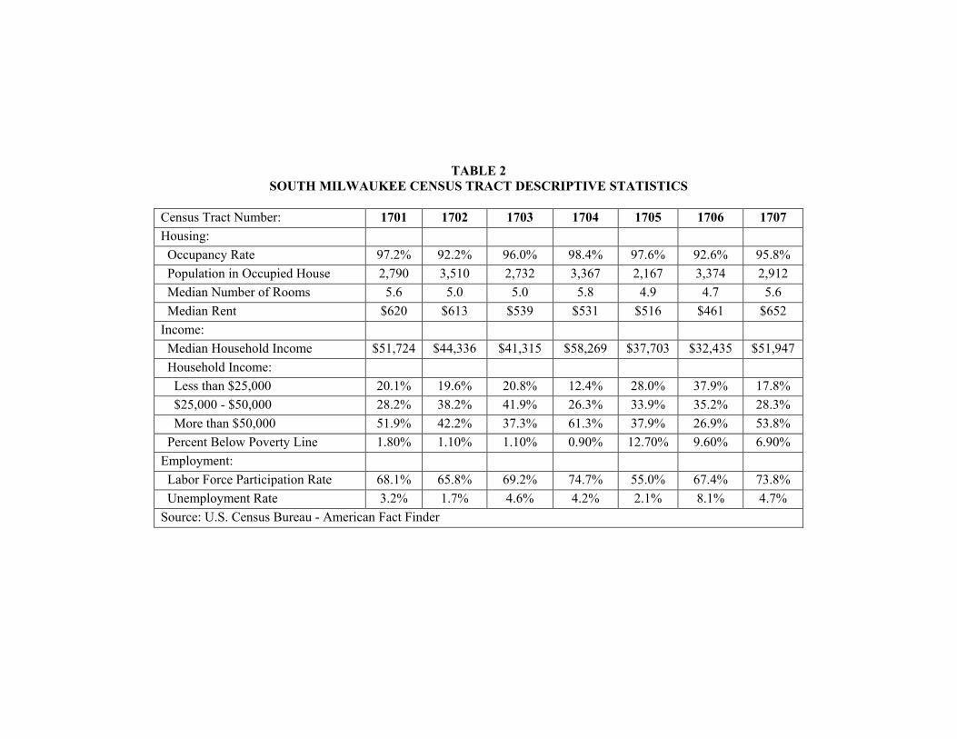
TABLE 2 SOUTH MILWAUKEE CENSUS TRACT DESCRIPTIVE STATISTICS

Census Tract Number: 1701 1702 1703 1704 1705 1706 1707 Housing: Occupancy Rate 97.2% 92.2% 96.0% 98.4% 97.6% 92.6% 95.8% Population in Occupied House 2,790 3,510 2,732 3,367 2,167 3,374 2,912 Median Number of Rooms 5.6 5.0 5.0 5.8 4.9 4.7 5.6 Median Rent $620 $613 $539 $531 $516 $461 $652 Income: Median Household Income $51,724 $44,336 $41,315 $58,269 $37,703 $32,435 $51,947 Household Income: Less than $25,000 20.1% 19.6% 20.8% 12.4% 28.0% 37.9% 17.8% $25,000 - $50,000 28.2% 38.2% 41.9% 26.3% 33.9% 35.2% 28.3% More than $50,000 51.9% 42.2% 37.3% 61.3% 37.9% 26.9% 53.8% Percent Below Poverty Line 1.80% 1.10% 1.10% 0.90% 12.70% 9.60% 6.90% Employment: Labor Force Participation Rate 68.1% 65.8% 69.2% 74.7% 55.0% 67.4% 73.8% Unemployment Rate 3.2% 1.7% 4.6% 4.2% 2.1% 8.1% 4.7% Source: U.S. Census Bureau - American Fact Finder

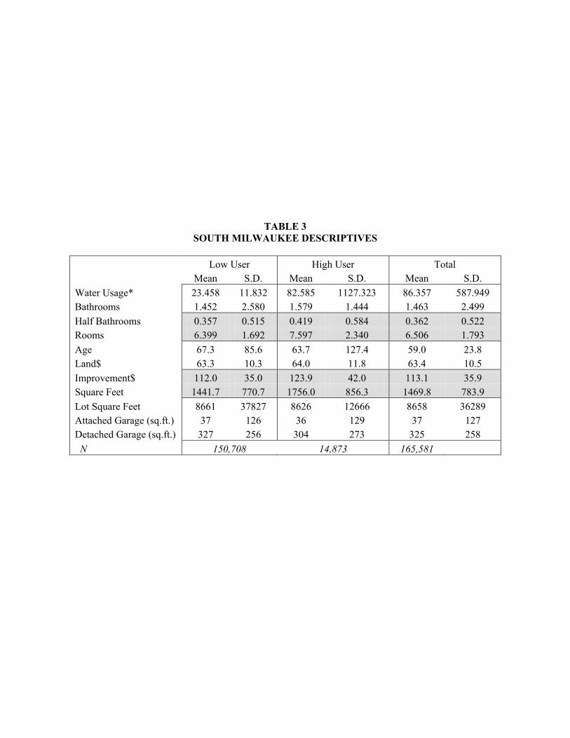
TABLE 3 SOUTH MILWAUKEE DESCRIPTIVES

Low User High User Total Mean S.D. Mean S.D. Mean S.D. Water Usage* 23.458 11.832 82.585 1127.323 86.357 587.949 Bathrooms 1.452 2.580 1.579 1.444 1.463 2.499 Half Bathrooms 0.357 0.515 0.419 0.584 0.362 0.522 Rooms 6.399 1.692 7.597 2.340 6.506 1.793 Age 67.3 85.6 63.7 127.4 59.0 23.8 Land$ 63.3 10.3 64.0 11.8 63.4 10.5 Improvement$ 112.0 35.0 123.9 42.0 113.1 35.9 Square Feet 1441.7 770.7 1756.0 856.3 1469.8 783.9 Lot Square Feet 8661 37827 8626 12666 8658 36289 Attached Garage (sq.ft.) 37 126 36 129 37 127 Detached Garage (sq.ft.) 327 256 304 273 325 258 N 150,708 14,873 165,581

TABLE 4 PROBIT ESTIMATION

Coef. S.E. Bathrooms 0.0034*** 0.0011 Half Bathrooms 0.0445*** 0.0094 Rooms 0.1271*** 0.0033 Age 6.626E-4*** 4.980E-5 Land$ -0.0035*** 5.619E-4 Improvement$ 0.0022*** 1.952E-4 Square Feet 2.289E-4*** 1.640E-5 Square Feet 2 -1.450E-8*** 1.640E-9 Square Feet Lot -2.270E-7 1.650E-7 Square Feet Lot 2 -7.800E-12*** 9.630E-13 Attached Garage -2.001E-4*** 4.000E-5 Detached Garage -1.183E-4*** 1.920E-5 Billing Period 2 -0.1552 0.0118 Billing Period 3 0.3299*** 0.1091 Tract 1702 (1600) -0.0264 0.0166 Tract 1703 (1800) 0.0309* 0.0171 Tract 1704 (1900) -7.511E-4 0.0172 Tract 1705 0.0447** 0.0198 Tract 1706 0.0150 0.0175 Tract 1707 -0.036 0.0182 Constant -2.6957*** 0.0435 R-Squared 0.0765

TABLE 5 SOUTH MILWAUKEE LOG-LOG ELASTICITY ESTIMATIONS

Low User High User OLS Census Tract Fixed Effects OLS Census Tract Fixed Effects Coef. S.E. Coef. S.E. Coef. S.E. Coef. S.E. Log Price -0.1646*** 0.0095 -0.1638*** 0.0218 -0.0357*** 0.0072 -0.0352*** 0.0094 Bathrooms -0.0014*** 4.332E-4 -0.0014 0.0010 -3.954E-4 0.0015 -4.853E-4 8.910E-4 Halfbath 0.0079* 0.0043 0.0076 0.0098 0.0161*** 0.0045 0.0154*** 0.0070 Rooms 0.0416*** 0.0014 0.0438*** 0.0024 0.0150*** 0.0013 0.0139*** 0.0026 Age -9.170E-5** 3.690E-4 -7.370E-5 1.251E-4 1.622E-4*** 1.780E-5 1.519E-4*** 1.570E-5 Land -0.0026*** 2.107E-4 -0.0028*** 6.304E-4 2.601E-4 2.801 E-4 4.853E-4 5.028E-4 Improvement 0.0020*** 1.585E-4 0.0018* 6.538E-4 2.542E-4*** 8.340E-5 3.408E-4** 1.895E-4 Square Feet 4.290E-5*** 7.820E-6 4.800E-5 2.770E-5 -4.410E-7 6.970E-6 6.620E-8 1.590E-4 Square Feet 2 -3.130E-9*** 6.230E-10 -3.280E-9 2.150E-9 -2.240E-10 6.370E-10 -3.380E-10 9.540E-10 Square Feet Lot 6.550E-8*** 2.480E-8 5.790E-8 3.830E-8 -6.920E-9 1.100E-7 4.020E-8 5.650E-8 Square Feet Lot 2 3.160E-12*** 3.860E-13 2.890E-12*** 8.630E-13 3.070E-12 9.890E-12 5.610E-12 1.540E-11 Attached Garage -5.640E-5*** 1.530E-5 -5.780E-5 9.500E-5 -5.620E-5*** 1.650E-5 -5.570E-5*** 1.650E-5 Detached Garage 5.600E-5*** 7.610E-6 6.070E-5* 3.050E-5 -3.050E-5*** 9.770E-6 -2.900E-5 2.050E-5 Billing Period 2 0.0037 0.0042 0.0038 0.0154 -0.0069 0.0064 -0.0074 0.0059 Billing Period 3 0.0848*** 0.0042 0.0849*** 0.0161 0.0047 0.0055 0.0041 0.0098 Constant 2.7121*** 0.0162 2.7205*** 0.0624 4.0987*** 0.0219 4.0813*** 0.0416 R-Squared 0.0343 0.0341 0.0250 0.0245