an estimated new keynesian model for israel · an estimated new keynesian model for israel eyal...
TRANSCRIPT

An Estimated New Keynesian
Model for Israel
Eyal Argov and David Elkayam December 2007 2007.08

An Estimated New Keynesian
Model for Israel
Eyal Argov and David Elkayam
December 2007 2007.08
The views expressed in this paper are those of the authors only, and do not necessarily
represent those of the Bank of Israel.
Email:
© Bank of Israel
Passages may be cited provided source is specified
Catalogue no. 3111507008/3
Monetary Department, Bank of Israel, POB 780, Jerusalem 91007
http://www.bankisrael.gov.il


An Estimated New Keynesian Model for Israel*
Eyal Argov and David Elkayam
Abstract
We formulate and estimate a small New Keynesian model for the Israeli economy. Our goal is to construct a small but still realistic model that can be used to support the inflation targeting process. The model contains three structural equations: An open economy Phillips curve for CPI inflation (excluding the housing component), an aggregate demand curve for the output gap and an interest parity condition for the nominal exchange rate. The model is closed with an interest rate reaction function (Taylor-type rule) and an ad hoc equation for the housing component of the CPI, which is dominated by exchange rate changes. In the specification of the model we had to pay special attention to the crucial role of the exchange rate in the transmission of monetary policy in Israel, which has a direct effect on almost 60 percent of the CPI. The model is estimated by the GMM method, using quarterly data for the period 1992:I to 2005:IV. In the estimation of the structural equations we tried to remain as close as possible to the theoretical formulation by restricting the dynamics to one lag at most. We use the model to characterize an "optimal" simple interest rate rule. We find that the monetary authority should respond to an hybrid backward-forward looking rate of inflation and does not benefit from direct reaction to exchange rate measures.
* This is a corrected version of the Hebrew discussion paper of February 2006. We would like to thank Michael Beenstock, Douglas Laxton, Akiva Offenbacher, and the participants of the seminars of the Monetary and Research Departments who's comments contributed to the paper. The views expressed in this paper are those of the authors only, and should not be interpreted as reflecting the views of the Bank of Israel.

4

5
יישום , קיינסיאני למשק קטן ופתוח-ניסוח ואמידה של מודל ניאו
למשק הישראלי
דוד אלקיים ואיל ארגוב
תמצית
המדיניות מעצבימקרו כלכלי קטן המיועד לסייע ל-בעבודה זו אנו מנסחים ואומדים מודל
רים בין המודל מתאר את הקש. הריבית הדרוש להשגת יעד האינפלציה שיעורהמוניטרית בקביעת
המשתנים העיקריים והחיוניים לתיאור מנגנון התמסורת של המדיניות המוניטרית במשק קטן
למעט סעיף (עקומת פיליפס לתיאור האינפלציה : המודל מכיל שלוש משוואות מבנה. ופתוח
משוואת ביקוש מצרפי ;שער החליפיןבפיחות הקצב של כפונקציה של פער התוצר ו,)הדיור
; כפונקציה של הריבית ושער החליפין הריאלי,ות פער התוצר במגזר העסקילתיאור התפתח
כפונקציה של הפער בין , לתיאור היקבעות שער החליפין של השקל ביחס לדולרUIPומשוואת
המתאר את (Taylor type rule)המודל נסגר באמצעות כלל ריבית. הריבית המקומית לעולמית
בניסוח . ציה של הפער שבין האינפלציה ליעדה ופער התוצר כפונקהבנק המרכזיקביעת ריבית
60- המשפיע ישירות על יותר מ,תפקיד המרכזי של שער החליפיןבהמודל הושם דגש מיוחד
המודל המנוסח בעבודה זו שייך לסוג המודלים שבהם . אחוזים של מדד המחירים לצרכן
נקודת המוצא למשוואות המודל :במילים אחרות. של הכלכלה" עמוקים"פרמטרים המודגשים ה
עם זאת כדי לחזק . בהינתן פונקציות תועלת וייצור, היחידות הכלכליותמצדהיא אופטימיזציה
מהמבנה , בניסוח משוואות המודל, סטינו לעיתים, של המודל) והאופרטיבי(את הצד האמפירי
תים הוספנו פיגור אחד ולעי, הוק למחירי הדיור-הוספנו משוואה אד – למשל (.י הצרוףהתיאורט
. GMMבשיטת , 2005:4 עד 1992:1נתונים רבעוניים לתקופה בהמודל נאמד ) .בחלק מהמשתנים
. באמצעות המודל הנאמד ניסינו לאפיין את המשתנים שרצוי לכלול בכלל התגובה של הריבית
גרסיבי ובאופן א, אינפלציה בדיעבד הלעאינפלציה הצפויה והן על הנמצא כי רצוי להגיב הן
לעמעבר לתגובה (שינויים בשער החליפין על נמצא שהתרומה של תגובה ישירה כנגד זאת. יחסית
.היא מועטה) אינפלציהה

6

7
1. Introduction In this paper we formulate and estimate a small New Keynesian model for the Israeli
economy. Our goal is to construct a small but realistic model that can be used for
forecasting, policy analysis, risk assessment and supporting the inflation targeting
process. The model contains three structural equations: A Phillips curve for consumer
price index inflation (excluding the housing component), an aggregate demand curve
for the output gap (in the business sector) and an interest parity condition for the
nominal exchange rate. The model is closed with an estimated reaction function
(Taylor-type rule) for the Bank of Israel's interest rate.
The model developed here is the smallest one which can be used to describe
the main ingredient of the transmission mechanism in a small open economy. An
important advantage of a small model is its simplicity and clarity, which help to
enhance the communication among the various groups that are related to the monetary
policy and its outcomes.
The theoretical framework and part of the empirical specification of the model
is based on the works of Svensson (2000), Adolfson (2001), Linde et al. (2004) and
Monacelli (2005). Our aim at this paper is to implement this framework in the context
of the characteristics of the Israeli economy and to arrive at a workable model that
could support the inflation targeting process.
The New Keynesian model in a closed economy contains (at least) three basic
equations: one for inflation, one for the output gap and one for the nominal interest
rate.1 In a small open economy the exchange rate has an important role in the
transmission mechanism of monetary policy. As described in Svensson (2000), the
exchange rate affects both the aggregate demand (output gap equation) and supply
(inflation equation) sides. On the demand side the exchange rate affects the relative
price of both imports and exports of goods and services. On the supply side it affects
consumer price directly, through the price of imported consumer goods which are part
of the consumption basket, and indirectly through the price of imported raw materials.
In the Israeli economy there is another important and unique channel through
which the exchange rate affect prices – by affecting the housing component of the
consumer price index (CPI). In the next section we shall describe this unique relation.
However, we note that this component constitutes about 20 percent of the CPI and 1 For an extensive presentation of the theory of the New Keynesian model in a closed economy see Woodford(2003). For theory and empirical implementation see Rotemberg and Woodford(1998).
8
that the pass-through from the exchange rate to this non-traded component is almost
immediate and complete.
In the analysis of inflation in an open economy one has to distinguish between
the prices of locally produced goods, which are mainly affected by aggregate demand,
and the prices of imported goods which are influenced directly by the exchange rate.
If one assumes a gradual pass-through from the exchange rate to import prices, then
one has to specify and estimate separate equations for the locally produced goods
(home goods) and for the imported goods (see, for example, Monacelli, 2005). In
most, if not all, empirical works, the New Keynesian Phillips Curve is estimated in
terms of the GDP deflator (for the home goods inflation equation) and the national
account's total import price deflator (for the imported goods inflation equation).2 In
this paper we concentrate on specifying and estimating an inflation equation in terms
of the CPI.3 The difficulty that one has to face is that the two components of the CPI
(i.e., locally produced goods and imported goods inflation) are unobservable. We try
to overcome this difficulty by specifying the imported goods inflation equation as a
distributed lag on the world import price inflation adjusted to exchange rate changes,
and augmenting this equation in the CPI inflation Phillips curve. Outcomes of such an
exercise are estimates of the price inflation of the two components, which could serve
as indicators in the analysis of the CPI inflation developments.
Another issue to which we pay attention in the specification and estimation of
the inflation equation is the distinction between the price of imported raw material
(which affects production costs) and the price of imported consumption goods (which
affects aggregate demand and consumption costs). This distinction, which is usually
neglected in most of the empirical works (Battini et al., 2005, is an exception),
enables us to asses the effect of a shock to the world's relative price of raw material.4
The main equations of the model are based on micro structure.5 As is well
known such an emphasis strengthens the theoretical consistency of the model but it
may weaken empirical aspects. In the estimation stage we tried to keep the
2 For examples, see Litemo (2006a), Batini et al. (2005) 3 There are several reasons that a CPI-oriented model will be more appropriate to the support of inflation targeting. At first the inflation target is in terms of CPI. Moreover the CPI is published with a relatively short lag and is not revised. 4 Such as a rise in the price of oil, which is an important (imported) raw material for the Israeli economy. 5 As will be detailed below, the output gap and inflation of locally produced goods are derived with DSGE formulation. The specification of the interest rate rule, the imported goods inflation equation and the housing price inflation equation are ad hoc.

9
specification of the estimated equations as close as possible to the DSGE formulation,
by starting with the DSGE specification and then allowing some additional dynamics,
whenever this seemed necessary, but restricting it to only one lag of the various
variables,6 which was found to strengthen the robustness of the estimated equations.
In the next section we present a short background of the economy. In Section
3 we develop the specification of the model's equations. In Section 4 we present and
discuss the estimation results. In Section 5 we describe the choice of the monetary
policy rule – based on simple optimization methods. Section 6 describes and discuss
the characteristics of the model and Section 7 offers conclusions.
2. A short background to the economy During the estimation period (1992 to 2005) the Israeli economy's real and nominal
sides experienced several major changes. A short description of those developments
will highlight several aspects with regard to the concrete implementation of the
theoretical framework. Specifically, we refer to the crucial role of the exchange rate in
the transmission process and the specific breakdown of the CPI inflation.
On the real side we can name the large immigration from the former Soviet
Union that resulted in an average yearly population growth of 3.6 percent during the
years 1990 to 1999. Another important development was the prolonged structural
change in the industrial sector: the high-tech industry grew rapidly while traditional
industries were stagnating.7
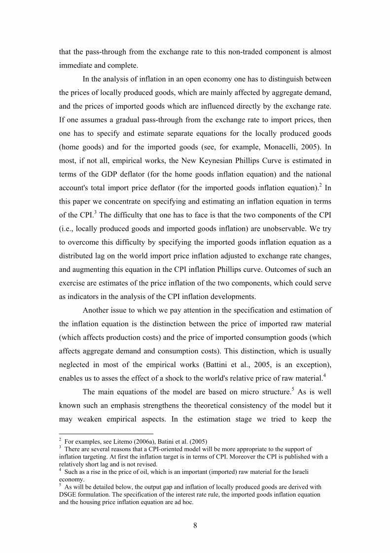
An important development in the nominal side was the declaration of inflation
targets in 1992, and the implementation of the inflation targeting regime since then.
During the years 1992 to 2000 inflation declined from a yearly rate of 9.4 percent to
0.0 percent. From 2001 to 2006 the average inflation rate was 1.6 percent, in the
lower part of inflation target band (1 to 3 percent). Another major development was
the transition to a flexible exchange rate regime that took place in the middle of 1997.
That development increased the sensitivity of the exchange rate to external shocks. As
a result the volatility of the exchange rate and (thereby) prices increased. On the other
hand, the transition increased the sensitivity of the exchange rate to the interest rate
6 In the ad hoc specification of the import price inflation we allowed two lags. 7 For example, see Justman (2002).

10
and thus enhanced the effectiveness of the interest rate as an instrument of stabilizing
the inflation and the output gap.8
Figure 1: Annual CPI inflation and the inflation target band, 1986-2006
As we shall see in section 4, despite the major changes that characterized the
Israeli economy during the estimation period, the rather standard New Keynesian
model fits the data rather well. This conclusion is based on the following: (1) the sign
and magnitude of most estimated parameters is in the range of the results obtained in
similar models for other economies. (2) A dynamic within sample simulation that
replicates fairly well the paths of the endogenous variables (except for the exchange
rate path). (3) Cross correlations produced from stochastic simulations of the model
are in line with the observed data.9
The Israeli economy is a very open economy10 and as can be expected the
exchange rate plays a major role in the transmission of monetary policy. As we shall
see in section 4, the pass-through from the exchange rate to import prices, and through
it to the CPI, is very high but still gradual, that is, part of the (direct) effect of the
8 For a survey on the exchange rate regimes during 1986 to 2005 see Elkayam (2003). 9 The dynamic simulation and cross-correlation comparison are presented in Argov et al. (2007). They are derived using a similar, though not identical, version of the model designated for practical use at the central bank. 10 In 2006 the ratio of export and import to GDP is 45 and 44 percents, respectively.
-4
-2
0
2
4
6
8
10
12
14
16
18
20
22
24
26
1986 1987 1988 1989 1990 1991 1992 1993 1994 1995 1996 1997 1998 1999 2000 2001 2002 2003 2004 2005 2006
YoY CPI Inflation
Inflation Target Band
%

11
exchange rate changes comes with a lag. As we shall see, assuming immediate pass-
through results in biased estimates of the inflation equation.
Figure 2: Quarterly Percent Change in the CPI Housing Component and the
Shekel/Dollar Exchange Rate , 1999-2006
In the Israeli economy, the exchange rate also has a direct effect on part of the
locally produced goods and services (even non-traded ones). That effect is a result of
practises that developed during the high inflation era (1974 to 1985), with inflation
reaching a yearly rate of 400 percent in 1984-85. One of the ways to avoid the
consequences of the high inflation was to link prices of goods and services to the
exchange rate of the shekel against the US Dollar.11 A relatively large market in
which that practise still exists is real estate (house prices and rents are nominated in
US Dollar and are linked to it, at least in the short- and medium-runs). The housing
component constitutes 20 percent of the CPI and since 1999 most of it is based on the
price of rented dwellings.12 In figure 2 we can see the high (and almost perfect)
correlation between the change in the housing component and the exchange rate
11 In 1985 a stabilization program took place and inflation declined to 16-21 percent in the years 1986 to 1992. Since 1999 the average yearly inflation rate has been 1.4 percent. 12 The CPI housing component is made of owner-occupied housing (77%), rental housing (20%) and other related expenditures (3%). The price of owner-occupied housing is measured by the rental equivalent approach (which is based on the rental market). As a result 97% of the CPI housing component is based on the price of rentals.
-8-7-6-5-4-3-2-10123456789
1999 2000 2001 2002 2003 2004 2005 2006
Quarterly change in CPI housing component
Quarterly change in NIS/USD exchange rate
%

12
changes. This unique relation, which complicates the inflation targeting process in
Israel, led us to specify and estimate a separate equation for the inflation of the
housing component (since 1999). The theory of the New Keynesian Phillips Curve
was applied to the CPI excluding housing.13
3. The theoretical model The model described below is largely based on Svensson (2000), Adolfson (2001) and
Linde et al. (2004). At several stages we deviate from other formulations, in order to
adjust the model to the special characteristics of the Israeli economy. For the sake of
completeness, and in order to highlight the meaning of the structural parameters that
we try to estimate, we shall present the main stages of the model's development, even
at the cost of some repetition of previous papers. For more background on the
formulations the reader is referred the papers above.
3.1 Households (output demand)
The domestic economy is populated by a continuum of infinitely-lived households
indexed by j, who consume Dixit-Stiglitz bundles of domestic and imported goods,
denoted htC and f
tC respectively. Domestic goods are produced by a continuum of
firms producing differentiated goods marked by index i. Let htiC )( denote the quantity
consumed of good i, and define:
11
0
1
)()1(−−
= ∫
h
h
h
h
diCC ht
ht i
ηη
ηη
,
where ηh > 1 is the elasticity of substitution between domestic goods.14 Cost
minimization, subject to a given level of domestic consumption ( htC ) leads to the
following demand function for good i:
hth
t
hth
t CP
PCh
ii
η−
=
)()()2( ,
13 We also excluded the fruit and vegetables component (whose weight in the CPI is 3.4 percent) as it is noisy and unpredictable. 14 A similar aggregating equation holds for the imported consumption bundle.

13
where htiP )( is the price of good i and the corresponding cost minimizing price
aggregator of locally produced goods is given by:
hh diPP h
th
t iη
η−
−
= ∫
11
1
0
1)( .
The composite consumption index is defined by:
11111
)()()()1()3(−−−
+−=
ηη
ηη
ηηη
η ft
cf
ht
cft CwCwC ,
where cfw is the long-run share of imports in consumption, and η is the elasticity of
substitution between imported and domestic goods. The corresponding minimum cost
price aggregator (consumer price index) is:
[ ] ηηη −−− +−= 11
11 ))(())(1()4( ft
cf
ht
cf
ct PwPwP ,
where htP and f
tP are the price aggregators of domestically produced and imported
goods, all in local currency units.
Household j’s contemporaneous utility depends on its own consumption
relative to lagged aggregate consumption 1−tC according to
( )σ
σ
−−
=−
−
1)(
11)(
)( ttt
hCCCu jj ,
where the parameter )1,0(∈h represents the extent of habit formation,15 and 1−σ is the
inter-temporal elasticity of substitution. Household j chooses a sequence of
consumption, domestic bond holdings and foreign bond holdings to maximize utility:
∑∞
=+
0t,,
)(Emax)5( )()()()(
kkt
k
BBCjCu
fttt jjj
β ,
subject to the flow budget constraint:
tct
ftt
ct
tc
ttt
ftt
ctt
tt j
jjjjj X
PB
PB
PiB
PiBC )(
)()()()()( 11
)1()1( )6( ++=
Φ++
++ −−
∗
εε ,
15 See Smets and Wouters (2003) and Christiano et al. (2005).

14
where tjB )( is household j’s holdings of one-period nominal bonds denominated in
the domestic currency; ftjB )( is its foreign counterpart denominated in the foreign
currency (dollar); tΦ is a risk premium paid on foreign assets; tε is the nominal
exchange rate (the price of foreign currency in terms of the domestic currency); tjX )(
is household j’s share of aggregate real profits in the domestic economy; ti and ∗ti are
domestic and foreign nominal risk-free interest rates, respectively (i.e., the domestic
bonds yield the gross return of )1( ti+ shekels and the foreign bonds yield the gross
return of )1( ∗+ ti dollars); β is the quarterly discount rate; and tE is the expectation
operator.
After aggregating the log-linearized first order conditions of the maximization
problem, one obtains the following equations (the Euler equation, the uncovered
interest parity condition, the optimal intra-temporal allocation across domestic and
imported goods bundles and the aggregate price level). Lower case letters denote log
deviation from steady state.
)E()1(
11
E1
1)7( 1t11tcttttt i
hhc
hhc
hc +−+ −
+−
−+
++
= πσ
ttttt iiee φ+−+= ∗+1tE)8(
)()9( ct
htt
ht ppcc −−= η
ft
cf
ht
cf
ct pwpwp +−= )1()10(
where te is the log of the nominal exchange rate; and ct
ct
ct pp 1−−=π is the CPI inflation
rate.16 Notice that in reality we do not have observations on the CPI components, htp
and ftp ; only c
tp is measurable. In the empirical part we shall try to overcome this
problem by assuming a specific structure of the imported inflation equation (we shall
return to that issue in the next subsection).
16 As discussed in the previous section πc is the CPI excluding housing, fruit and vegetables. Below, describing monetary policy, we will mark the overall CPI by πcpi.

15
Assuming the demand for world trade is characterized by the same intra-
temporal elasticity of substitution, η , the demand for the local economy's exports, htx ,
is given by:17
)()11( ∗∗ −−−= tthtt
ht pepyx η ,
where ∗ty is the world's trade and *
tp is the price of consumer goods in the foreign
economies. Following Monacelli (2005), we assume that in the export sector, prices
are flexible and follow the law of one price (L.O.P.). Therefore tht ep − is the export
price in foreign economies' currency (dollars).
Let us define the real exchange rate as: ctttt pepq −+= ∗)12( .
Following Adolfson (2001) and Munacelli (2005), we assume that the pass-
through from the exchange rate and the relevant world prices to the import price at the
local market is gradual. Let us define ctψ as a temporary deviation from the law of
one price (L.O.P. gap), that is:
)()13( ttf
tct epp +−= ∗ψ .
Log-linearization of the national account identity yields: htxgc
htx
htg
htct invxgcy )1()14( γγγγγγ −−−+++= ,
where ty is the output gap, htg and h
tinv are the log deviations from equilibrium of
public consumption and investment (both in value added terms), and iγ is the long-
run share in output of component i.
Using equations (7)-(14) we derive the output gap equation:
17 h
tx is also a continuum of differentiated goods with constant elasticity of substitution ηh, similar to equation (1).

16
. E1
11
E1
11
)1(
E1
11
E1
11)1(
)(
E1
11)1(
)()E(
)1()1(
1E
11)15(
1t11t1
1t11t1
1t11t11t
+−
+−+
+−
+−−−−+
+−
+−+
+−
+−
−+
+
+−
+−
−+
+−+−
−+
++
=
∗+
∗−
∗+−
+−+−
+−+−+
tttxht
ht
htxgc
ht
ht
htg
ct
ct
ctc
f
xccf
tttcf
xcfcc
ttc
ttt
yh
yh
hyinvh
invh
hinv
gh
gh
hghh
hw
w
qh
qh
hqw
wi
hhy
hhy
hy
γγγγ
γψψψγγη
γγηπ
σγ
Equation (15) can be written more compactly as: ∗
+ +++++−= txhtinv
htgttq
ctttit yavniagaaqaEiaya )))))) ψπ ψ)()15( 1 .
where for any variable xt ( ∗t
ht
htttt yinvgqy , , , ,,ψ ) we define
11 11
1 −+ +−
+−= ttttt x
hxE
hhxx) .
and:
xxxgcinvggc
f
xcfc
qc
i aaaw
wa
hha γγγγγ
γγησγ
=−−−==−
+=
+−
−= );1(;;)1(
)(;
)1()1( .
Equation (15a) illustrates the basic variables determining the output gap: the
real interest rate, the real exchange rate, the temporary deviation from the L.O.P,
government spending, investments and world trade, all in deviation form. Notice that
we still have to specify how the L.O.P. gap, ctψ , is measured.
3.2 Domestic producers (inflation equation)
Following Rotemberg (1982) domestic firms face menu costs. They choose a price
sequence to minimize the cost of price changes and the cost of deviating from their
flexible price. Formally all firms face the following problem:
{ }[ ]∑
∞
=−++++ −+−
∞=+ 0
21
2t
)()()ˆ(Emin)16( )()()()(
0 τττττ
τδττ
ht
ht
ht
ht
ipiiii ppcpp
ht
,
where htip )( is the price set by the domestic firm i; h
tip )(ˆ is the optimal flexible price
(i.e., the price that would have been chosen in the absence of adjustment costs); and δ
is a discount factor.
The first order condition for the firm's minimization problem is given by:

17
( ) ( )ht
ht
ht
ht
ht
ht iiiiii pp
cpppp )()()()()()( ˆ1E)17( 1t1 −+−=− +− δ ,
where htip )(ˆ is solved from profit maximization under flexible prices:
tz
th
tinv
tht
gt
htt
xt
ht
htZPP
iiiii ZPINVPGPXPCPt
xt
ht iii
)()()()()( ˆˆ max)18()()()( ,ˆ ,ˆ
−+++ ε ,
ht
ht
ht
htt INVGXCYts iii +++= )()()(..)19( ,
[ ] θθ
−−− ==111 )()()20( )()()()(
zf
zf wf
twh
ttt iiii ZZZY .
Constraint (19) is the aggregate output identity and (20) is the production
function. htiZ )( and f
tiZ )( are intermediate domestic and imported inputs respectively. z
tP is the aggregate price of intermediate inputs and zfw is the share of imports in
intermediate goods. We assume the price and quantity of government spending and
investments are given to each firm identically and exogenously.
Solving the flexible price optimization problem given in (18)-(20), and using
the local demand function (2) and its equivalent for exports, yields the optimal
flexible price (in log-linear form, averaged across all firms):
tzt
ht ypp
θθ−
+=1
ˆ)21( .
The RHS side of (21) is the log deviation of nominal marginal costs, where the cost
minimizing input price aggregator is given by: zft
zf
zht
zf
zt pwpwp +−= )1()22( ,
where zhtp and zf
tp are the prices of domestic and imported inputs to production (in
domestic currency).
Following Svensson (2000) we assume that the local price of inputs is similar
to it's consumer counterpart: ht
zht pp =)23( .
Averaging (17) across all firms, and plugging in (21)-(23) we arrive at the
following equation for the inflation in the domestically produced consumption goods:

18
)(1
1E)24( 1tht
zft
zf
tht
ht pp
cw
yc
−+−
+= + θθπδπ .
This equation is distinct from the basic closed-economy New Keynesian
model in that the real price of imported inputs affects inflation as well as the output
gap. This is a source of influence of the exchange rate on domestic prices.
Now, following Gali and Gertler (1999), we assume that only a fraction λ of
the firms set their price accordingly, while a fraction (1–λ) use a simple rule of
adjusting their price according to last period's domestic inflation. We also assume
δ=1, and get:
)(1
1)1(E)25( 11tht
zft
zf
tht
ht
ht pp
cw
yc
−+−
+−+= −+ λθ
θλπλπλπ .
Recall that neither zftp nor h
tp are observable. In the following we shall write
)( ht
zft pp − as a sum of three components: the first is exogenous and measurable
)( ∗∗∗ −= tzt
zct ppp , The second is endogenous and measurable, tc
f
qw )1(
1−
, and the third,
ctc
f
cfz
t ww
ψψ)1( −
+ , is not measurable, and we shall have to use a proxy for it.18
Applying this separation on equation (25) we get:
−++
−++
−+−+= ∗
−+ctc
f
cfz
ttcf
zct
zf
tht
ht
ht w
wq
wp
cw
yc
ψψλθ
θλπλπλπ1)1(
11
1)1(E)26( 11t,
where ∗∗∗ −= tzt
zct ppp represents a temporary deviation (from trend) in the world's
relative price of inputs. ztψ is the L.O.P. gap in the inputs sector and defined by:
)()27( tzt
zft
zt epp +−= ∗ψ .
Equation (26) is the Phillips curve for the inflation in locally produced goods.
As mentioned earlier inflation components are unobservable and therefore it is
impossible to directly estimate equation (26). We will use equation (10) in first
difference to eliminate the local inflation in favor of total inflation ( cπ ) and imported
inflation ( fπ ): 18 For derivation of equation (26) see appendix A.

19
[ ] . )1(E 1)1(
1)1(1
1)1()1(E)28(
11t
11t
ft
ft
ft
cf
ctc
f
cfz
ttcf
zct
zfc
ftcf
ct
ct
ct
ww
wq
wp
cw
wyc
w
−+
∗−+
−−−+
−++
−+−+
−−+−+=
πλπλπ
ψψλθ
θλπλπλπ
Now equation (13), in first difference, can be used to replace the (unobserved)
imported inflation by it's determinants – the change in world import prices of
consumer goods ( ∗∆ tp ), nominal depreciation ( te∆ ) and the change in the L.O.P gap
( ctψ∆ ):
[ ] , ))(1()EE( 1)1(
1)1(1
1)1()1(E)29(
111t1t
11t
ctt
ctt
ctt
cf
ctc
f
cfz
ttcf
zct
zfc
ftcf
ct
ct
ct
decdecdecww
wq
wp
cw
wyc
w
−−++
∗−+
∆+−−∆+−∆++
−++
−+−+
−−+−+=
ψλψλψ
ψψλθ
θλπλπλπ
where ttt epdec ∆+∆= ∗ .
Our next step is to specify an equation for the local prices of imported
consumer goods ( ftp ) which will define the L.O.P. gap ( c
tψ ). One possibility is to
assume immediate (and complete) pass-through, that is: ∗+= ttf
t pep (as in Svensson,
2000, for example). In that case 0=ctψ and equation (29) is fully measurable. A more
reasonable possibility is to follow Adolfson (2001) and Munacelli (2005), who
assumed price stickiness in imported goods as well as in the domestic goods.
Consequently a dynamic equation arises, linking the imported goods inflation, ftπ , to
its real marginal cost ctψ . Direct estimation of such an equation is possible only if
there exist data on both the local and imported goods in the CPI. However, typically
there are no statistics on this separation. One approach, taken in Leitemo (2006a) and
Linde et al. (2004), is to use the national accounts deflators. For htπ they used the
GDP price deflator and for ftπ they used the import price deflator. However, this kind
of approach is not free of problems. First, the pricing theory above relates to market
prices, i.e., either consumer prices or producer prices, so the components of the CPI or
the WPI are more relevant than the national account deflators. Second, at least in
Israel, the quarterly data of the national accounts are noisy and relatively unreliable in
comparison with CPI series. Thirdly, the inflation target is in terms of the CPI. For
these reasons we choose to estimate an equation in terms of the CPI alone.

20
The solution we choose is in the spirit of Adoldson (2001) and Munacelli
(2005), but rather ad hoc. We assume that ftp and zf
tp evolve according to the
following distributed lag process, through which we can calculate ctψ and z
tψ :
))(1()()()EE()30( 2232111321t1t1 −∗−−
∗−
∗+
∗+ +−−−++++++= tttttttt
ft epepepepp αααααα ,
))(1()()()EE()31( 2232111321t1t1 −∗−−
∗−
∗+
∗+ +−−−++++++= t
ztt
ztt
ztt
zt
zft epepepepp αααααα .
Namely, we assume the existence of some rigidities in the price setting of imported
goods so that the final price ( ftp or zf
tp ) is influenced partly by the expected relevant
world price (adjusted for exchange rate currency), partly by the contemporaneous
level and partly by the first two lags. In the following we shall estimate the α1, α2 and
α3. Of course, we can add more leads or lags to this equation and test their
significance. The choice of the first two lags is based on empirical results.
Using these assumptions we can characterize the L.O.P. gaps in the imported
consumption goods and imported intermediate inputs as follows:
1321211t1 )1()1(E)32( −+ −−−−−−−= tttct decdecdec ααααααψ ,
1321211t1 )1()1(E)33( −+ −−−−−−−= tttzt dezdezdez ααααααψ ,
where ttt epdec ∆+∆= ∗ and tztt epdez ∆+∆= ∗ .
Plugging (32) and (33) in equation (29) we derive a fully observable equation
for the CPI (excluding housing, fruit and vegetables) inflation. In the equation below
all the parameters can be identified and estimated:
[ ]
[ ] , )1(
)1()1(E)1(
1)1(
)1()1(E)34(
232113211
1321211t1
11t
−−+
−+∗
−+
−−−++++
−−−−−−−+−
+−+
−+−+=
ttttcf
ttttcf
zctq
cf
tycf
ct
ct
ct
cedcedcedcedw
zcedzcedzcedqw
pbw
ybw
((((
&&&&&&&&&
αααααα
ααααααλ
λπλπλπ
where tcf
cf
tt decw
wdezzced
)1( −+=&&&
1-1t1tt E)1(EE −+ −−−= ττττ λλ decdecdecced( .
The non-structural parameters are:
cw
bc
bzf
qy =−
=)1( θ
θ .

21
3.3 Foreign currency market (the exchange rate equation)
We start with the UIP condition derived from the households' first order conditions
(equation 8). Accordingly, the spot nominal exchange rate is affected by future rate
expectations, exp1+t
e , and the adjusted interest rate differential:
tttt iieet
φ+−+= ∗
+
exp1
)'8( .
Preliminary experiments showed that lags of the exchange rate, and foreign
and local interest rates also contribute to the explanation of the spot exchange rate.
Accordingly, we assume that households' expectations with respect to the exchange
rate are partly rational and partly adaptive, where ω measures the degree of
rationality:19
1texpexp E)1()35(
1 ++−=+ tt eee
tωω .
Combining (8)' with (35) yields the following equation for the exchange rate:
11111t )1())(1()()1(E)36( −−∗−
∗−+ −−+−−−−+−+= ttitttttt iiiieee φωφωωω .
3.4 Monetary policy (interest rate rule)
We assume that the central bank follows an inflation forecast based rule of the form:
1,4 ])([)1()37( −+ +++−++⋅−= titzty
Tt
cpitt
Tttit izyEri κκκππκπκ θπ ,
where cpit
cpit
cpit pp 4
,4−+++ −= θθθπ is year-on-year overall inflation rate at t+θ, T
tπ is the
inflation target, rt is the natural real interest rate and zt represents additional variables
that might enter the rule. The inflation forecast horizon is θ quarters. Notice that while
the behavioral model related only to the CPI excluding housing, fruits and vegetables,
the forecast relates to the overall CPI (excluding only fruit and vegetables). The
motivation is clear: the inflation target is defined on overall inflation and therefore
monetary policy is likely to react to overall inflation. In order to close the model a
simple, ad hoc, equation will be specified and estimated for the CPI housing
component. In the next sections we will devote detailed discussion on the estimated
rule's parameters, the possibility of including the exchange rate in the rule and the
choice of θ.
19 A similar approach was taken by Leitemo and Soderstrom (2005b).

22
Table 1: The Model Equations
The (non-housing) inflation equation (33):
[ ]
[ ] , )1(
)1()1(E)1(
1)1(
)1()1(E)1.(
232113211
1321211t1
11t
−−+
−+∗
−+
−−−++++
−−−−−−−+−
+−+
−+−+=
ttttcf
ttttcf
zctq
cf
tycf
ct
ct
ct
cedcedcedcedw
zcedzcedzcedqw
pbw
ybwF
((((
&&&&&&&&&
αααααα
ααααααλ
λπλπλπ
where tc
f
cf
tt decw
wdezzced
)1( −+=&&&
11-t1tt E)1(EE −+ −−−= ττττ λλ decdecdecced( .
The housing price inflation equation:
132110)2.( −+ ∆+∆+∆+= tttthouset ebebeEbbF π .
The CPI identity: ct
houset
CPItF πππ ⋅+⋅≡ 8.02.0)3.( .
The output gap equation: ∗
+ ++++−= txhtinv
htgtq
ctttit yavniagaqaEiayF ))))) )()4.( 1π ,
where for any variable xt ( ∗t
ht
httt yinvgqy , , , , ) we define 11 1
11 −+ +
−+
−= ttttt xh
xEh
hxx) ,
and the estimated parameters are:
xxxgcinvggc
f
xcfc
qc
i aaaw
wa
hha γγγγγ
γγησγ
=−−−==−
+=
+−
−= );1(;;)1(
)(;
)1()1( .
The nominal exchange rate:
)]()1()[()()1()5.( 11111 −∗−
∗+−+ −−−−+−−+=− tttttttttt iiiieEeeEeF ωωφω .
The interest rate equation:
1111,4
2)(
2)(
2)(
)()1()6.( −−
∆−−
+ +
∆+∆+
++
++−++⋅−= ti
tte
ttq
tty
Tt
cpitt
Tttit ieeqqyy
EriF κκκκππκπκ θπ,
where: ∑−=
++ =θ
θθ ππ
3
4
i
cpiitt .

23
4. Estimation of the model The estimation is based on quarterly data between 1992:I and 2005:IV. The variables
that were used for the local economy, Israel, are: the consumer price index (excluding
housing, fruit and vegetables), the CPI housing component, the shekel/dollar nominal
exchange rate, the effective Bank of Israel nominal interest rate, business sector
product, gross investment, government purchases and the forward 5-to 10-year real
yield on government indexed bonds (which serves as a proxy for the time varying
natural rate of interest). For the foreign economy we used: the unit value of imported
consumer goods and imported inputs to production, the one-month LIBID dollar
interest rate and the industrial country's volume of imports (to approximate world
demand). In addition, the unit value of industrialized country's imports was used as an
instrumental variable. In order to construct the gap variables the Hodrick-Prescott
filter was employed. More information on the data, their source and constructing the
final variables is available in Appendix B.
For convenience we summarized the operative equations of the model in Table
1. Each equation was estimated separately by the GMM method. In the estimation
procedure, we assume rational expectations, meaning all variables indexed t+1 or t+2
are replaced with the actual variable in that quarter.
4.1 Estimation of the inflation equation
The inflation equation was derived in Section 3 above and can be viewed in table 1
equation (F.1) . The estimated equation is related to CPI excluding housing, fruit and
vegetables. To the estimated equation we added a constant (which turned out
insignificant) and seasonal dummy variables. The estimation results seem more robust
when replacing the leveled variables with moving averages. Therefore, the output gap
term (yt) and the real price of imported inputs (all terms in curly brackets) were
replaced with a two period moving average; for example, instead of yt we used
)(5.0 1−+⋅ tt yy . All variables were multiplied by 4, so the dependent variable is the
annualized quarterly inflation.

24
Table 2: Estimation of the Inflation Equation (F.1) Estimation for the period 1992:I-2005:IV (56 observations)*
Gradual pass-through
excluding 1998:III
F.1c
Gradual
pass-through
F.1b
Immediate
pass-through
F.1a
0.565 (14.8)
0.591 (12.6)
0.580 (17.5)
λ
0.556 (5.4)
0.464 (4.7)
0.091 (12.3)
cfw
0.102 (2.0)
0.086 (2.2)
0.018 (1.6)
by
0.030 (1.1)
0.039 (1.3)
0.122 (6.12)
bq
0.123 (3.7)
0.097 (2.3)
0.0 α1
0.416 (15.6)
0.424 (13.6)
1.0 α2
0.328 (19.2)
0.337 (16.4)
0.0 α3
0.849 0.822 0.792 R2
2.15 2.31 2.42 S.E.
2.38 3.08 2.65 DW
0.237 (0.951)**
0.231 (0.953)**
0.252 (0.996)**
Jstat
* The numbers in parenthesis are t-statistics. ** The number in parenthesis is the p-value for the test where the null hypothesis is that the over identifying restrictions are satisfied. The statistic for the test, JT ⋅ , is asymptotically 2χ with degrees of freedom equal to the number of over identifying restrictions (number of instruments less estimated parameters).
As mentioned above, in the estimation procedure, we replaced the variables
that represent expectations with thier actual realizations. As a result, the unexpected
factor of each such realization is included in the error term of the estimated equation,
and these elements are potentially correlated with any variable that appears at the
same date (including the exogenous variables). For example, we replaced 1+ttdecE and

25
21 ++ tt decE with 1+tdec and 2+tdec , respectively. As a result, any variable dated t+1 or
t+2 cannot serve as an instrument. Notice that the above equation includes tt decE 1−
which is replaced by tdec . As a result, only lags of the various variables (including the
exogenous variables) can be incorporated in the set of the instrumental variables.
Throughout, the sets of instrumental variables for each estimation are documented in
Appendix C.
We begin by assuming immediate (perfect) pass-through from the exchange
rate and world prices to the domestic import price, i.e., we assume 0== zt
ct ψψ . In
equation (F.1) this means 0, 31 =αα and 12 =α .
The estimates of the parameters of equation (F.1a) under the immediate pass-
through assumption are presented in the first column of table 2.20 As is evident from
the table, the equation has a good explanatory power, all the estimates have the right
sign, and apart from by, all are significant (at the 5 percent significance level).
However, for the weight of imports in consumption goods ( cfw ) we obtained an
estimate of 0.09, which appears too small. We would expect a value closer to 0.4.
Earlier trials with several alternative specifications suggested that the bias in this
estimate may be related to the presumably false assumption of immediate (perfect)
pass-through. To account for this, we proceeded by assuming that the pass-through in
the prices of imported goods (consumer goods and inputs to production) is gradual
and of the form of equations (30) and (31), which means that the L.O.P. gaps in
imported consumer goods and imported inputs are in the form of equations (32) and
(33). Hence we will estimate the α parameters.
The estimates of equation (F.1b) when assuming gradual pass-through are
presented in the second column of table 2. As we can see, the parameters α1, α2 and α3
are significant, supporting the hypothesis of gradual pass-through. Furthermore, both
the weight of imports in consumption and the coefficient of the output gap are larger,
and of a magnitude closer to what we would expect. The weight of imports we obtain
is 0.46, which is of the order of magnitude we would expect. However this estimation
seems to deliver some extent of serial correlation.21 It is found that omitting the third
20 Under the assumption of complete pass-through, Et-1dect is not included in the equation and thus we can include exogenous variables dated at t in the instrumental variables set. 21 This can be inferred from the high value (close to 3) of the Durbin-Watson statistic. although this statistic does not provide a formal test in our case.

26
quarter of 1998 (equation (F.1c) in the third column of Table 2) relieves much of the
serial correlation without changing the magnitude of the estimated parameters.
The reason that 1998:III is problematic lies in the unexpected 15%
depreciation of the currency in the last quarter of that year (following the LTCM
crisis). That depreciation was behind the 5% increase in the CPI in that quarter. Under
the assumption of rational expectations, we use the actual inflation of 1998:IV as an
unbiased proxy for the inflation expectations generated in 1998:III. Obviously, it is a
poor proxy in that quarter and as a consequence caused the undesired serial
correlation.
A possible means for assessing the reasonability (of the order of magnitude) of
the estimated parameters is to compare to other similar works. However, the
comparison is not trivial since the specification of the equations is not exactly the
same in all papers. Further more, we compare different economies in different time
periods. Nevertheless, we choose three works in which the parameters were estimated
by classical methods: Lopez (2003) estimated a model for Colombia, Caputo (2004)
estimated a model for Chile, and Leitemo (2006a) estimated a model for the UK. In
the following comparison we shall use the estimates of equation (F.1b) in Table 2.
Table 3 summarizes the comparison.
Table 3: Cross Country Comparison of the Inflation Equation
Leitemo
England
GDP deflator
Caputo
Chile
CPI
Lopez
Colombia
CPI
Equation
F.1b
CPI
Parameter
0.580 0.562 0.352 0.591 Coefficient of
expected inflation
0.067 0.027 0.086*0.5 =
0.051
output gap affect on
the CPI
0.07 0.086
output gap affect on
the domestic prices
by
- 0.035 - 0.039
Coefficient of real
exchange rate
bq

27
First we shall compare the coefficient of expected inflation (λ in equation
F.1). As can be seen the estimate here (0.591) is quite similar to that of Caputo
(0.562) and Leitemo (0.580) and larger than that obtained by Lopez (0.352).
Regarding the coefficient of the output gap, our estimate with regard to CPI inflation
is similar to the one obtained by Caputo and larger than the one obtained by Lopez.
Litemo estimated equation using the GDP deflator and got a value of 0.067. The
analogous value here is (by) 0.086.
As for the real exchange rate coefficient, it can only be compared with Caputo
(2004), which estimated 0.035 in comparison to 0.039 here.
4.2 Estimation of the CPI housing component equation
The above equation relates to the inflation of the CPI excluding the housing and fruit
and vegetables components. Since the inflation target is in terms of the overall CPI we
need to specify and estimate an equation for the housing component as well. As is
evident from Figure 2 (Section 2), this component is influenced mainly by the
(shekel/dollar) exchange rate developments. Based on this we estimated equation
(F.2a) where the housing component inflation ( housetπ ) is explained by the (current,
lead and lagged) exchange rate depreciations ( e∆ ), a constant, and seasonal dummy
variables (not reported). All variables were multiplied by 4, so that the dependent
variable is the annualized quarterly CPI housing component inflation. The equation
was estimated by GMM. The resulted estimates are shown in Table 4.
For purposes of the model's long run properties and convergence, in the
simulations we will use an homogeneous version of the equation (exchange rate
coefficients sum to one) in which we omit the lead of the exchange rate. This ensures
that monetary policy will not have a permanent effect on the relative price of housing.
The estimation results of the restricted equation (F.2b) are presented in the second
column of Table 2.

28
Table 4: Estimation of CPI Housing Component Inflation Equation (F.2) Estimation for the period 2000:I-2006:III (27 observations) *
Without lead
homogeneous restriction
F.2b
With lead
F.2a
-0.833
(-2.4)
-0.979
(-4.17)
b0
0.0 0.166
(1.76)
b1
0.864
(54.85)
0.774
(18.14)
b2
1- b2 0.148
(3.77)
b3
0.936 0.923 R2
2.834 3.243 S.E.
1.91 1.53 DW
0.315 (0.383)**
0.312 (0.209)**
Jstat
* The numbers in parenthesis are t-statistics. ** The number in parenthesis is the p-value for the test where the null hypothesis is that the over identifying restrictions are satisfied. The statistic for the test, JT ⋅ , is asymptotically 2χ with degrees of freedom equal to the number of over-identifying restrictions (number of instruments less estimated parameters).
4.3. Estimation of the output gap equation (F.4)
Estimation of the output gap equation, allowing for gradual pass-through of the form
described in equation (32), did not yield reasonable results. This need not necessarily
indicate the lack of gradual pass-through, but rather signals weak identifying power
when it appears only in levels terms (in the output gap equation). Hence, we shall
proceed to estimate the equation under the assumption of immediate pass-through. For
the sake of simplicity we shall write the final output gap equation (15) in a compact
form (F.4), where all parameters can be identified and estimated. The equation is
further simplified by defining, for any variable xt ( ∗t
ht
httt yinvgqy , , , , ),

29
11 11
1 −+ +−
+−= ttttt x
hxE
hhxx) , i.e., tx) is the deviation of tx from a weighted average of
its lead and lag.
In the following, we added a constant (which turned out insignificant in the
first three versions) and seasonal dummy variables to the various estimated equations.
In the estimation, the annualized real interest rate gap was divided by 4, so as to
express all variables in quarterly term. The equation was estimated by GMM method.
The estimation results of equation (F.4a) are presented in the first column of
Table 5. The results show an intermediate value of "habit persistence" (0.542). We
used the estimated value of cfw from the inflation equation (F.1b) (in Table 2) in order
to derive estimates of the structural parameters (σ, η and γc).
Comparing the estimated parameters that express-long run shares in GDP (γx,
γg, γinv, and γc) with the actual average share we find that the consumption share is
estimated accuratly. However, the estimated share of exports seems too low
(estimated 0.156 compared to 0.3 actual) and the share of government purchases
seems too high (estimated 0.225 compared to 0.06 actual). We should note that what
we call 'actual' is not necessarily the correct parameter. The long-run shares relate to
the components of the GDP in value added terms, for which actual data are not
available. The assessment regarding the value of the 'actual' is based on each
component's share in total uses. In the second column of Table 5 (equation F.4b), we
present estimates of the equation when imposing that assessment with regard to the
actual shares. As can be seen, the estimated values of the other parameters remain
quite similar to those in equation (F.4a).
In equations (F.4c) and (F.4d) we present estimates analogous to (F.4a) and
(F.4b) when eliminating habit persistence. i.e., under the constraint that h=0. As can
be seen, under this restriction the explanatory power of the equation is reduced, the
coefficient of the interest rate (ai) increases, and that of the real exchange rate (bq)
decreases.
In Table 6 we compare the estimated parameters of (F.4a) to those obtained by
Lopez (2004), Caputo (2004) and Leitemo (2006a). As can be seen, the coefficients of
expected output gap, and of the real exchange rate are larger, here, than those
obtained in the other papers.

30
Table 5: Estimation of the Output Gap Equation (F.4)
Estimation for the period 1992:I-2005:IV (56 observations) *
With output weight
restrictions, h = 0 (F.4d)
No output weight
restrictions, h = 0 (F.4c)
With output weight
restrictions, with h (F.4b)
No output weight
restrictions, with h (F.4a)
0.0 (-)
0.0 (-)
0.542 (5.9)
0.542 (5.9) h
-0.703 (-7.4)
-0.819 (-6.2)
-0.399 (-4.07)
-0.424 (-3.5) ai
0.060 (1.5)
0.125 (2.6)
0.173 (4.2)
0.268 (5.6) aq
0.30 (-)
0.392 (7.1)
0.30 (-)
0.156 (1.5) ax
0.06 (-)
0.222 (6.3)
0.06 (-)
0.225 (5.4) ag
0.16 (-)
0.167 (7.4)
0.16 (-)
0.139 (7.7) ainv
Solving for deep parameters by plugging in 464.0=cfw .
0.683 (7.4)
0.266 (2.5)
0.336 (3.5)
0.336 (2.8) σ
0.062 (1.5)
0.136 (2.7)
0.275 (5.6)
0.379 (3.8) η
0.48 (-)
0.218 (3.3)
0.48 (-)
0.480 (4.5) γc
0.536 0.503 0.699 0.712 R2
2.50 2.67 2.04 2.05 S.E.
2.66 2.59 3.01 2.90 DW
0.261 (0.974)**
0.257 (0.937)**
0.221 (0.988)**
0.221 (0.964)**
Jstat
* The numbers in parenthesis are t-statistics. ** The number in parenthesis is the p-value for the test where the null hypothesis is that the over identifying restrictions are satisfied. The statistic for the test, JT ⋅ , is asymptotically 2χ with degrees of freedom equal to the number of over-identifying restrictions (number of instruments less estimated parameters).

31
Table 6: Cross Country Comparison of the Output Gap Equation
Leitemo
England
Caputo
Chile
Lopez
Columbia
Equation
(F.4a)
parameter
0.53 0.453 0.109 0.649 h+1
1
-0.28 - -0.668 -0.424 ai
0.11 0.016 0.002 0.268 aq
0.25 0.026 0.092 0.156 ax
4.5. Estimation of the exchange rate equation
since the middle of 1997 the Bank of Israel has not intervened in the foreign exchange
market, so that the exchange rate has been determined by market forces. The final
exchange rate equation (35) was modified assuming that the unobserved risk premium
is a fixed parameter (see equation F.5).22 The equation was estimated by GMM
method for the period 1997:III to 2005:IV. The annualized interest rate differentials
were divided by 4. The results are summarized in table 7.
Table 7: Estimation of the Exchange Rate changes Equation (F.5) Estimation for the period 1997:III-2005:IV (34 observations) *
ω 0.569
(9.53)
φ 3.383
(2.43)
R2 0.428 S.E. 2.52 DW 2.78 Jstat 0.114
(0.693)**
* The numbers in parenthesis are t-statistics. ** The number in parenthesis is the p-value for the test where the null hypothesis is that the over identifying restrictions are satisfied. The statistic for the test, JT ⋅ , is asymptotically 2χ with degrees of freedom equal to the number of over-identifying restrictions (number of instruments less estimated parameters).
The parameter of the future exchage rate is estimated to be 0.569, and the
estimate of the average annualized risk premium is 3.383 percent. Additional
22 In the estimated equation et is 100*log(Nominal Exchange Rate).

32
experiments hint at the possibility that the average risk premium declined towards the
end of the estimation period, concurrent with the decline in the inflation rate.
4.6. Estimation of the interest rate rule
We considered equation (F.6) where in addition to the inflation gap, )( ,4 Tt
cpittE ππ θ −+ ,
the monetary authority may react directly to the output gap, the real exchange rate gap
and the nominal depreciation (all in terms of two quarters moving average). The
equation was estimated by GMM, and the instrumental variables are listed in
Appendix C. The equation was estimated with various θ ranging from 0 to 4.23 Only
for θ equal to 0 and 1 did we receive reasonable and stable results. A possible
explanation of that result is that the actual yearly inflation for three and four quarters
ahead is a "bad" estimate of expected inflation, due to the large fluctuations of the
inflation rate during the estimation period. When we replaced actual ex-post yearly
inflation with one-year-ahead inflation expectations which are derived from the
capital market (CM), we obtained better results. As can be seen in Table 8 the
estimated equations using CM expectations is not "worse" (in terms of fit) even than
those that use yearly inflation with θ equal to 0 and 1.
In the first three columns of Table 8 we present the results of the estimated
equations under the restrictions: κq = 0, κ∆e = 0, that is, without the real exchange rate
gap or exchange rate changes. As can be seen, for the outcome based rule (i.e, for
θ=0) we get for the inflation gap a coefficient greater than one (1.39), a positive and
significant coefficient for the output gap (0.233), and a coefficient of 0.772 for the
lagged interest rate. When we move yearly inflation one quarter ahead (i.e, for θ=1)
the coefficients of the inflation and output gaps increase but the inertia also increases.
When we use CM expectations instead of actual inflation (which can be interpreted as
moving to θ=4) the coefficients of the inflation and output gaps increase further but
the inertia reduces to a similar rate of that in the case of θ=1.
In the last three columns of Table 8 we present the results when we add the
real exchange rate gap and the exchange rate changes to the equations. For the
estimates of the parameters κi , κπ , κy the results are analogous to those in the first
three columns. The effect of the exchange rate gap is significant in the three equations
and the exchange rate changes is significant in F.6d and F.6f. 23 The use of a smoothed measure of inflation and the restriction of θ to at most 4 quarters ahead is based on the conclusions of the paper by Levine et al. (2003).

33
According to the results above it seems that the Bank of Israel reacted to the
exchange rate, in addition to the inflation and output gaps. The natural question is
why? Is it because exchange rate fluctuations appear as a factor in its loss function?
Alternatively, is it because reducing the exchange rate fluctuations helps to reduce the
fluctuations of the inflation and or the output gap? In the next section we shall use the
model to answer that question. However the main challenge of the next section is to
choose the value of the parameters of a forecast-base rule for the model.
Table 8: Estimation of the Interest Rate Equation (F.6) Estimation for the period 1992:III-2005:IV (54 observations) *
CM
(F.6f)
θ = 1
(F.6e)
θ = 0
(F.6d)
CM κq = κ∆e = 0
(F.6c)
θ = 1 κq = κ∆e = 0
(F.6b)
θ = 0 κq = κ∆e = 0
(F.6a)
0.806 (33.0)
0.873 (35.4)
0.804 (35.8)
0.807 (29.7)
0.876 (29.6)
0.772 (40.3) κi
2.841 (6.55)
1.619 (3.37)
1.255 (9.91)
3.391 (7.23)
2.526 (4.13)
1.390 (9.97) κπ
0.625 (4.02)
0.764 (3.06)
0.448 (3.60)
0.397 (3.55)
0.330 (1.83)
0.233 (2.80) κy
0.452 (2.37)
1.120 (2.90)
0.422 (2.83) -- -- -- κq
0.193 (5.02)
0.121 (1.47)
0.083 (2.12) -- -- -- κ∆e
0.944 0.932 0.944 0.943 0.927 0.945 R2
1.03 1.13 1.02 1.02 1.15 1.00 S.E.
1.73 1.54 1.57 1.74 1.85 1.69 DW
0.181 (0.939)**
0.224 (0.794)**
0.166 (0.941)**
0.229 (0.903)**
0.228 (0.872)**
0.203 (0.925)**
Jstat
* The numbers in parenthesis are t-statistics. ** The number in parenthesis is the p-value for the test where the null hypothesis is that the over identifying restrictions are satisfied. The statistic for the test, JT ⋅ , is asymptotically 2χ with degrees of freedom equal to the number of over-identifying restrictions (number of instruments less estimated parameters).

34
5. Deriving an Optimal Simple Monetary Policy Rule In this section we will search for an optimal-simple monetary policy rule, simple in
the sense that the rule takes the form of equation (F.6), optimal in the sense that it will
be based on a central bank loss function (to be defined below). Specifically, we would
like to choose the inflation forecast horizon (defined by the θ parameter) and test
whether the model justifies direct reaction to the exchange rate.
The simulations held for this purpose consists of the following equations:
a. The inflation equation (F.1b) which allows for gradual pass-through.
b. The housing component equation (F.2b), adjusted for long run convergence to the
general inflation target. This insures that the model converges – relative prices are
constant in the long run, and that monetary policy can not affect the long run relative
price of housing.
c. The output gap equation (F.4a) which allows for habit formation in consumption
and does not impose restrictions on the weights of the GDP components.
d. The exchange rate equation, modified in two manners. First, we found that
allowing the forward weight (ω) to be greater than 0.5 embodies potential
determinacy problems. Therefore we reduced the weight to 0.45.24 Second, we
assume an exogenous varying risk premium rather than a constant term.25
e. An auto regressive equation for all exogenous variables to account for their
dynamics. In general the equations were estimated by OLS. For details on these
equations see Argov et al. (2007).26
f. In order to perform stochastic simulations, standard deviations must be defined for
each shock (equation residual). These were based on the estimated equations. In all
simulations we assume absence of monetary policy shocks and a constant inflation
target. Details on the standard deviations are presented in Appendix D.
The objective of monetary policy is to minimize the variation in
macroeconomic variables.27 To get a first taste, Table 9 presents the standard
deviation of key model variables under various values of θ, i.e., the inflation forecast
24 In Argov et al. (2007) ω was estimated to be 0.45 in a similar specification. In their estimation a larger set of instrumental variables was used. 25 The risk premium variable was taken from Hecht and Pompushko (2006). 26 Section 7. 27 To be even more exact – to minimize variation of macroeconomic variables around their flexible price level.

35
horizon.28 In these simulations we used the first three parameter estimates from
equation F.6f (κi = 0.81, κπ = 2.84, κy = 0.63); we assumed no direct reaction to the
real exchange rate nor the nominal depreciation (κq, κ∆e = 0). The last row of Table 9
is the following weighted sum of variance:
)(0.4)(5.0)(0.1 iVaryVarVarL cpi ∆⋅+⋅+⋅= π .
This weighted sum (L) will later serve as the monetary policy's loss function. The
weights in L are somewhat non-standard; in particular, the interest rate weight is
usually chosen to be less than unity.29 In our case, the weights were chosen so that the
standard deviations under the simple-optimal rules fall in the neighborhood of those
under the empirical (estimated) rules. Specifically, only interest rate weights far
greater than 1 generate interest rate variations close to those observed in the data.
Table 9: Standard Deviations of Main Variables Using Estimated Parameters
Under Various Forecast Horizons κi =0.81, κπ =2.84, κy =0.63
θ = 3 θ = 2 θ = 1 θ = 0 S.D. of variable1
4.23 3.86 3.72 3.75 πcpi
4.52 4.13 3.94 3.92 πc
3.77 3.95 4.15 4.35 y
1.02 1.04 1.02 1.00 ∆i
3.80 3.90 4.02 4.15 q
8.75 8.75 8.86 9.09 ∆e
29.16 27.02 26.61 27.52 Weighted Sum of
Variance2
1. Inflation and depreciation rates are annualized, ∆i is quarterly change in annualized interest rate. 2. 1.0*Var(πcpi) + 0.5*Var(y) + 4.0*Var(∆i). 28 θ = 0 is a backward-looking rule, θ = 1,2 are hybrid backward-forward-looking rules and θ = 3 is a forward-looking rule. Current inflation is included in each rule. For details see equation (F.6). 29 For example Svensson (2000) uses a value of 0.01, Leitemo and Soderstrom (2005b) use 0.1.

36
It is evident from the table that the greater the forecast horizon, the smaller are
the variance in the output gap, the real exchange rate and nominal depreciation (up to
θ = 2). In contrast, the standard deviation of CPI inflation is lowest with a one-period-
ahead forecast horizon (θ = 1). The standard deviation of interest rate changes is not
very sensitive to the forecast horizon. To a large extent, these are the result of the fast
and strong pass-through from exchange rate shocks to CPI prices.30 Following such
shocks, inflation rises sharply for one quarter. The peak in year-on-year inflation is in
the second quarter. Therefore, the longer the forecast horizon the quicker the interest
rate starts re-adjusting to its pre-shock level, and a smaller output sacrifice is
generated. Immediate and direct reaction to the peak of year-on-year inflation (θ = 1)
minimizes the variance in quarterly inflation.
It is seen that the loss function L is minimized with θ = 1, i.e., using a hybrid
backward-forward-looking inflation measure of one-period-ahead inflation
expectations, current inflation and two lags of inflation realizations. θ = 1 being
superior to θ = 0 and θ = 3 is rather robust to the loss function choice (it holds as long
as the weight on the output gap is smaller than 1.75 and the weight on the interest rate
is smaller than 33!). However it is somewhat harder to distinguish between θ = 1 and
θ = 2. If the loss function weight on the output is 0.8 then θ = 2 is superior.
Table 10 presents standard deviations of key variables (and a weighted sum)
using θ = 1 and the parameters of estimated equation (F.6f) when gradually allowing
for direct reaction to the nominal and real exchange rates.
It is seen that direct reaction to the level of the real exchange rate (κq > 0)
reduces the variance in inflation while raising the variance in output. In part, this is
due to the dominance of shocks that generate a negative correlation between the real-
exchange-rate and the output gap, for instance, nominal exchange rate and foreign
interest rate shocks. Therefore it is found by the weighted sum to be sub-optimal (as
long as the output weight in L is bigger than 0.25). Direct reaction to the nominal
depreciation (κ∆e > 0) slightly improves the variance in inflation while generating
moderately larger interest rate and output standard deviations. In sum, it does not
seem to contribute much to central bank performance. The results outlined here for
θ = 1 hold for other θ values as well.
30 Due to the dollarized housing price component and a rather short import price pass-through lag structure (see equation 30).

37
Table 10: Standard Deviations of Main Variables Using Estimated Parameters
and Implications of Direct Reaction to the Exchange Rate, κi =0.81, κπ =2.84, κy =0.63, θ = 1
κq = 0.45 κ∆e = 0.19
κq = 0.00 κ∆e = 0.19
κq = 0.45 κ∆e = 0.00
κq = 0.00 κ∆e = 0.00
S.D. of variable1
3.51 3.64 3.59 3.72 πcpi
3.81 3.94 3.80 3.94 πc
4.48 4.18 4.49 4.15 y
1.10 1.06 1.05 1.02 ∆i
4.24 3.96 4.35 4.02 q
8.55 8.56 8.85 8.86 ∆e
27.19 26.48 27.38 26.61 Weighted Sum of
Variance2
1. Inflation and depreciation rates are annualized, ∆i is quarterly change in annualized interest rate. 2. 1.0*Var(πcpi) + 0.5*Var(y) + 4.0*Var(∆i).
Having the results of Tables 9 and 10 in mind we turn to formally derive an
optimal-simple rule, based on minimizing the loss function L. We take the following
steps:
a. We find the inflation and output reaction measures (κπ, κy) that minimize the
loss function while restricting the smoothing parameter (κi) to 0.831 and the
exchange rate reaction parameters (κq, κ∆e) to zero.
b. Taking the optimal parameters found in step (a), we minimize the loss
function by means of the exchange rate reaction parameters. In this we
follow the approach taken by Leitemo and Soderstrom (2005b).
c. For comparison purposes we optimize on all four parameters (κπ, κy, κq, κ∆e).
d. Steps (a)-(c) are repeated for each forecast horizon (θ = 0,1,2,3).
31 Optimizing on all three parameters drives the optimal parameters to unreasonable areas in which the reaction and smoothing parameters are very high, especially when the forecast horizon grows. Since it was found in this study, like others, that a smoothing parameter value of 0.8 reflects central banks' actual conduct, we chose to fix it to this value.

38
Tables 11-14 report the optimized parameters, the resulting standard deviations
and loss function values. For comparison, we found that using the globally optimal
interest rate rule (assuming commitment), the loss function value is 24.10.
Similar to what we found with the estimated rule, the hybrid backward- and
one-period-ahead forward-looking rule (θ = 1) seems to deliver the lowest (optimized)
loss function values. In this case we found the optimal inflation reaction parameter
(κπ) is 2.93, larger than what was found in the estimation assuming a short forecast
horizon. Similar to the estimation, we learn from the tables that as the forecast horizon
increases, the optimal inflation reaction parameter grows.
The optimal output gap reaction parameter (κy) is 0.9, again higher than the
estimated values. This result might have a simple operational reason: the model
assumes perfect knowledge of the current state of the output gap; of course, in reality,
not only does the central bank not know the true measure of the gap, it does not even
have a precise real-time HP filter estimate due to lags in data publication and well
documented end-of-sample filtering problems.
For all forward looking rules (θ > 0) we find that direct reaction to exchange
rate measures does not contribute in reducing the loss function. In some cases the
optimized parameters are negative! We conclude that the forecast of CPI inflation
summarizes the relevant information, even in a very open economy, even when some
inflation components are eccentrically linked to the exchange rate. In contrast, we find
some benefit in nominal exchange rate reaction in backward-looking rules (θ = 0).
Based on these results we will employ a simple optimal rule with θ = 1, κi =
0.8, κπ = 2.93, κy = 0.5 and no direct reaction to exchange rate measures. The output
gap reaction parameter was reduced from the one found in the optimization procedure
due to the operational considerations mentioned above. This rule generates a loss
function value of 26.8, only 1.4% higher than the best of the optimal simple rules
found above and 11.1% higher than the globally optimal (commitment) rule.

39
Table 11: Optimal Forecast-Based Rules, Standard Deviations of Main Variables
and Loss Function2,3
θ = 0
Optimizing on:
κπ , κy , κq , κ∆e
Optimizing on: κ∆e
Optimizing on: κq
Optimizing on:
κi , κπ , κy
0.80 0.80 0.80 0.80 κi
2.54 2.81 2.81 2.81 κπ
1.03 0.99 0.99 0.99 κy
0.18 -- 0.16 -- κq
0.24 0.24 -- -- κ∆e
S.D. of
variable1
3.77 3.73 3.78 3.83 πcpi
4.03 3.99 3.95 4.00 πc
4.04 4.08 4.11 4.04 y
1.05 1.07 1.05 1.04 ∆i
3.95 3.94 4.07 4.01 q
8.69 4.68 9.07 9.10 ∆e
26.78 26.83 27.16 27.21 Loss
Function Value2
1. Inflation rates are annualized, ∆i is quarterly change in annualized interest rate. 2. We find the κ parameters that minimize the objective function: 1.0*Var(πcpi) + 0.5*Var(y) + 4.0*Var(∆i) 3. For all simulations, κi is fixed on 0.8.

40
Table 12: Optimal Forecast-Based Rules, Standard Deviations of Main Variables
and Loss Function2,3
θ = 1
Optimizing on:
κπ , κy , κq , κ∆e
Optimizing on: κ∆e
Optimizing on: κq
Optimizing on:
κi , κπ , κy
0.80 0.80 0.80 0.80 κi
2.81 2.93 2.93 2.93 κπ
0.90 0.90 0.90 0.90 κy
0.02 -- 0.01 -- κq
0.12 0.12 -- -- κ∆e
S.D. of
variable1
3.71 3.68 3.72 3.73 πcpi
3.98 3.96 3.95 3.96 πc
3.96 3.98 3.96 3.95 y
1.09 1.11 1.09 1.09 ∆i
3.89 3.90 3.94 3.93 q
8.66 8.66 8.84 8.84 ∆e
26.40 26.41 26.48 26.48 Loss
Function Value2
1. Inflation rates are annualized, ∆i is quarterly change in annualized interest rate. 2. We find the κ parameters that minimize the objective function: 1.0*Var(πcpi) + 0.5*Var(y) + 4.0*Var(∆i) 3. For all simulations, κi is fixed on 0.8.

41
Table 13: Optimal Forecast-Based Rules, Standard Deviations of Main Variables
and Loss Function2,3
θ = 2
Optimizing on:
κπ , κy , κq , κ∆e
Optimizing on: κ∆e
Optimizing on: κq
Optimizing on:
κi , κπ , κy
0.80 0.80 0.80 0.80 κi
3.38 3.12 3.12 3.12 κπ
0.80 0.81 0.81 0.81 κy
-0.13 -- -0.05 -- κq
-0.09 -0.06 -- -- κ∆e
S.D. of
variable1
3.76 3.81 3.79 3.78 πcpi
4.04 4.07 4.08 4.06 πc
3.87 3.86 3.85 3.87 y
1.14 1.12 1.14 1.14 ∆i
3.87 3.89 3.84 3.87 q
8.77 8.77 8.68 8.68 ∆e
26.94 26.96 26.97 26.98 Loss
Function Value2
1. Inflation rates are annualized, ∆i is quarterly change in annualized interest rate. 2. We find the κ parameters that minimize the objective function: 1.0*Var(πcpi) + 0.5*Var(y) + 4.0*Var(∆i) 3. For all simulations, κi is fixed on 0.8.

42
Table 14: Optimal Forecast-Based Rules, Standard Deviations of Main Variables
and Loss Function2,3
θ = 3
Optimizing on:
κπ , κy , κq , κ∆e
Optimizing on: κ∆e
Optimizing on: κq
Optimizing on:
κi , κπ , κy
0.80 0.80 0.80 0.80 κi
3.20 3.46 3.46 3.46 κπ
0.93 0.99 0.99 0.99 κy
0.16 -- 0.12 -- κq
0.06 0.04 -- -- κ∆e
S.D. of
variable1
4.05 4.03 4.02 4.05 πcpi
4.36 4.35 4.33 4.36 πc
3.69 3.64 3.67 3.68 y
1.18 1.22 1.22 1.19 ∆i
3.81 3.75 3.82 3.78 q
8.58 8.56 8.62 8.61 ∆e
28.81 28.85 28.84 28.85 Loss
Function Value2
1. Inflation rates are annualized, ∆i is quarterly change in annualized interest rate. 2. We find the κ parameters that minimize the objective function: 1.0*Var(πcpi) + 0.5*Var(y) + 4.0*Var(∆i) 3. For all simulations, κi is fixed on 0.8.

43
6. The model's impulse response functions In this section we present dynamic elasticities (impulse responses) of the endogenous
variables, with respect to each of the following shocks: monetary policy, nominal
exchange rate and the output gap (demand shock). The simulations are based on
equations (F.1b), (F.2b), (F.4a) and (F.5) as described in Section 5. To close the
model we used the "optimal" simple rule of Section 5. (The parameters of the rule are:
θ = 1, κi = 0.8, κπ = 2.93, κy = 0.5, κq = 0.0 and κ∆e = 0.0.) In addition, we will present
the same impulse responses when monetary policy is operated according to estimated
equation (F.6a). This alternative employs a backward-looking rule (θ = 0) and less
aggressiveness in reaction to inflation and the output gap. In the following we shall
refer briefly to some interesting characteristics of the model, that can be inferred from
the impulses.
Figure 6.1 presents impulse responses with respect to one percentage point
(p.p.) shock to the nominal interest rate. Notice that all the endogenous variables are
immediately affected by the shock and that the immediate response is the largest.
Usually in estimated models one would expect to find a hump-shaped response of
inflation and the output gap to the interest rate shock. The large and quick response of
the endogenous variables in this model is partly due to the existence of the exchange
rate channel and the large immediate exchange rate pass-through. The unexpected
increase in the interest rate causes an immediate decline of the exchange rate which
immediately affects inflation and the real exchange rate, and through it – the output
gap. Another reason for the quick response is the relatively large coefficients of
expectations in the inflation, output gap and exchange rate equations (that is, the large
degree of which the model is forward-looking).
In figure 6.2 we present the impulse responses with respect to an unexpected
10-percentage-points (p.p.) shock to the exchange rate. Notice that here as well (as in
figure 6.1), the immediate response is the largest. Due to the concurrent positive
response of the interest rate, the 10 p.p. shock ends in only a 7.5 p.p. devaluation in
the first quarter. Concurrently, CPI inflation increases by 2.5 p.p, indicating
immediate pass-through of 1/3 with respect to the CPI inflation. The nominal interest
rate increases immediately by 0.5 p.p. and peaks at 0.9 p.p. above the steady state (in
the baseline simulation). The real rate temporarily drops in the first quarter; however,
as the nominal rate continues to rise and inflation re-converges, the real rate peaks at

44
1.2 p.p. two quarters following the shock. As a consequence, output falls for two
years, where the peak is two quarters after the shock.
In the alternative simulation with the empirical monetary policy rule, the
interest rate path is 0.2 p.p. lower for three periods. As a result, inflation and output
are higher. In addition, we notice that the interest rate starts reverting down to the
steady state one period after the baseline case. This is due to the backward-looking
nature of the policy rule. The year-on-year inflation measure used in the rule drops
four quarters after the shock – the time in which the interest rate reverts to steady
state. Ceteris paribus, this causes a deeper output gap reaction.
The above simulations highlight the role of the exchange rate in the
transmission mechanism of monetary policy in an open economy. The high exchange
rate pass-through means high sensitivity of the inflation rate to shocks to the exchange
rate. On the other hand, the high exchange rate pass-through also enhances the
effectiveness of the nominal interest rate as a tool for stabilizing inflation.
In figure 6.3 we show the impulse responses with respect to a shock in the
output gap equation. In the first quarter the nominal interest rate increases in the
intention to stabilize output. This causes an immediate decrease of the exchange rate,
which sets off the inflationary effect of the demand shock so that year-on-year
inflation is soon below the steady state. This open-economy feature demonstrates the
policy tradeoff between stabilization of output and inflation in light of demand-side
shocks. This calls for a careful choice of the output gap reaction parameter. As can be
seen from the alternative simulation, empirically, interest rates reacted less to output
gaps, leaving some more short-run inflationary pressures.

45
Figure 6.1: Impulse Response Function to 1 p.p. Interest Rate Shock With optimal-simple rule (baseline) Vs. estimated rule (alternative)
i – Nominal interest rate r – Real interest rate πcpi – Quarterly CPI inflation (annualized) π4cpi – Year on year CPI inflation y – output gap q – real exchange rate gap ∆e – Quarterly depreciation rate (annualized) e – (log) Nominal exchange rate _base – Baseline simple-optimal rule _alt – Alternative estimated rule

46
Figure 6.2: Impulse Response Function to 10 p.p. Exchange Rate Shock With optimal-simple rule (baseline) Vs. estimated rule (alternative)
i – Nominal interest rate r – Real interest rate πcpi – Quarterly CPI inflation (annualized) π4cpi – Year on year CPI inflation y – output gap q – real exchange rate gap ∆e – Quarterly depreciation rate (annualized) e – (log) Nominal exchange rate _base – Baseline simple-optimal rule _alt – Alternative estimated rule

47
Figure 6.3: Impulse Response Function to 1 p.p. Output Gap Shock With optimal-simple rule (baseline) Vs. estimated rule (alternative)
i – Nominal interest rate r – Real interest rate πcpi – Quarterly CPI inflation (annualized) π4cpi – Year on year CPI inflation y – output gap q – real exchange rate gap ∆e – Quarterly depreciation rate (annualized) e – (log) Nominal exchange rate _base – Baseline simple-optimal rule _alt – Alternative estimated rule
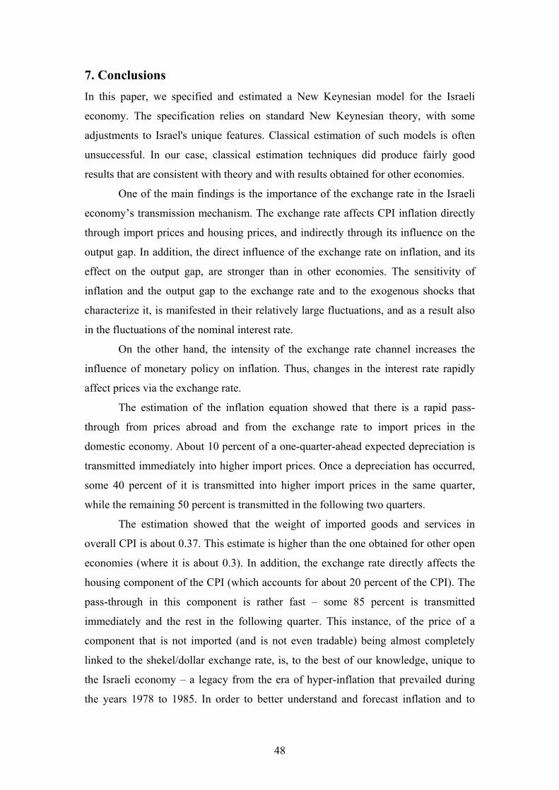
48
7. Conclusions In this paper, we specified and estimated a New Keynesian model for the Israeli
economy. The specification relies on standard New Keynesian theory, with some
adjustments to Israel's unique features. Classical estimation of such models is often
unsuccessful. In our case, classical estimation techniques did produce fairly good
results that are consistent with theory and with results obtained for other economies.
One of the main findings is the importance of the exchange rate in the Israeli
economy’s transmission mechanism. The exchange rate affects CPI inflation directly
through import prices and housing prices, and indirectly through its influence on the
output gap. In addition, the direct influence of the exchange rate on inflation, and its
effect on the output gap, are stronger than in other economies. The sensitivity of
inflation and the output gap to the exchange rate and to the exogenous shocks that
characterize it, is manifested in their relatively large fluctuations, and as a result also
in the fluctuations of the nominal interest rate.
On the other hand, the intensity of the exchange rate channel increases the
influence of monetary policy on inflation. Thus, changes in the interest rate rapidly
affect prices via the exchange rate.
The estimation of the inflation equation showed that there is a rapid pass-
through from prices abroad and from the exchange rate to import prices in the
domestic economy. About 10 percent of a one-quarter-ahead expected depreciation is
transmitted immediately into higher import prices. Once a depreciation has occurred,
some 40 percent of it is transmitted into higher import prices in the same quarter,
while the remaining 50 percent is transmitted in the following two quarters.
The estimation showed that the weight of imported goods and services in
overall CPI is about 0.37. This estimate is higher than the one obtained for other open
economies (where it is about 0.3). In addition, the exchange rate directly affects the
housing component of the CPI (which accounts for about 20 percent of the CPI). The
pass-through in this component is rather fast – some 85 percent is transmitted
immediately and the rest in the following quarter. This instance, of the price of a
component that is not imported (and is not even tradable) being almost completely
linked to the shekel/dollar exchange rate, is, to the best of our knowledge, unique to
the Israeli economy – a legacy from the era of hyper-inflation that prevailed during
the years 1978 to 1985. In order to better understand and forecast inflation and to

49
reliably estimate the exchange rate /CPI relation, we found it worthwhile to separate
the housing component from the CPI and to estimate a separate equation for it.
Also, in the case of the output gap equation it was found that the exchange rate
(in this case, the real exchange rate) has a larger effect than that found in similar
studies of other economies. This finding is further evidence of the Israeli economy’s
degree of openness and its sensitivity to exogenous global shocks.
The estimation of the inflation and output gap equations yielded a high
coefficient for the expectations term (0.6 and 0.65 respectively). This indicates a low
degree of inertia in both variables.
In most economies, a relatively long lag is found in the influence of the
interest rate on inflation. In contrast, our study found that the transmission mechanism
from the interest rate to inflation in the Israeli economy is rapid, even in comparison
to other small open economies. This finding is a result of two factors: 1) the
immediate effect of the interest rate on the exchange rate and the strong and rapid
effect of a depreciation on inflation; 2) the high coefficients obtained for the
expectation variables in the equations for inflation and the output gap. The strong
influence of expectations in these two equations is consistent with the New Keynesian
theory, which emphasizes the importance of the public’s expectations in the
transmission mechanism.
In the search for a simple optimal monetary policy rule we found two policy
implications: (1) regardless of the strong and fast exchange rate channel described
above, the central bank does not gain much by directly reacting to its (nominal or real)
innovations. The CPI inflation provides enough information for conduct of monetary
policy. (2) Due to the fast transmission from shocks and interest rates to inflation, and
the low persistence characterizing it, monetary policy should be based on a hybrid
backward-forward-looking measure of inflation.

50
Appendix A – Deriving Equation (26) Equation (25) is a hybrid local prices Phillips Curve in which inflation dynamics are
determined by the output gap and the real price of imported inputs.
)(1
1)1(E)25( 11tht
zft
zf
tht
ht
ht pp
cw
yc
−+−
+−+= −+ λθ
θλπλπλπ .
For practical purposes (since htp is unobservable) we shall re-write the last
term. First let us add and subtract ftp , the local price of imported consumption goods:
)()()()A.1( ht
ft
ft
zft
ht
zft pppppp −+−=− .
Next we shall use the definition of ctp given in equation (10), in order to
eliminate htp :
)()1(
1)()()A.2( ct
ftc
f
ft
zft
ht
zft pp
wpppp −
−+−=− .
Next we can use the general definition of incomplete pass-through given in
equations (13) and (27):
−++−+
−+−=− ∗∗∗ c
tcf
cfz
tctttc
ft
zt
ht
zft w
wpep
wpppp ψψ
1)(
)1(1)()()A.3( .
Finally we define the relative price of imported production inputs
)( ∗∗∗ −= tzt
zct ppp and use the definition of the real exchange rate (12):
−++
−+=− ∗ c
tcf
cfz
ttcf
zct
ht
zft w
wq
wppp ψψ
1)1(1)()A.4( .
In this form )( ht
zft pp − is a sum of three components: the first, ∗zc
tp , is
exogenous and measurable, The second, tcf
qw )1(
1−
, is endogenous and measurable,
and the third, ctc
f
cfz
t ww
ψψ)1( −
+ , is not measurable and for it we shall have to use a
proxy. Plugging (A.4) in equation (25) we derive equation (26):
−++
−++
−+−+= ∗
−+ctc
f
cfz
ttcf
zct
zf
tht
ht
ht w
wq
wp
cw
yc
ψψλθ
θλπλπλπ1)1(
11
1)1(E)26( 11t .

51
Appendix B – Description of the Data The estimation of the model used three types of data: gaps, rates of change and
interest rates. This appendix will describe each type and its source. In general,
quarterly rates of change and interest rates are annualized while the gaps are
expressed in conventional quarterly terms. However, in the estimation of each
equation we normalize all variables to the same term, thus allowing the direct
interpretation of the estimated parameters.
1. Gaps
All the gaps were calculated using the HP filter. In what follows, we denote the
smoothing of series X using the HP filter as HP(X). The gap of the original series Z
(for example, business sector real output) is denoted by z (the output gap) and is
calculated as follows:
[ ] 100*))(log(HP)log()B.1( ZZz −= .
The term in square brackets is the deviation rate of Z from its trend.
Multiplying by 100 expresses the gap in percent.
Following is a description of the gaps included in the model:
y – the output gap which is based on the business sector real GDP (Y) . The
trend was calculated using data starting from 1968:I. Source: Bank of Israel (BoI)
database.
gh – the public consumption gap which is based on the real purchases
component of the public sector (Gh). The trend was calculated using data starting from
1964:I. Source: BoI database.
invh – the investment gap which is based on real gross investment (INVh). The
trend was calculated using data starting from 1964:I. Source: BoI database.
y* – the world trade gap which is based on the real imports of the
industrialized countries32 (Y*). The trend was calculated on the basis of data starting in
1960:I. Source: the IFS database. The IFS database series contains a break in 1996:I
due to a definition change. Therefore the IFS yearbook and older versions of the
series were used to chain data before 1996 to the reliable database series following
1996.
32 Volume of imports divided by unit value.

52
q – the real exchange rate gap is based on the real exchange rate (Q) which is
calculated as follows:
ct
tc
tt P
PQ ε⋅=
∗
)B.2( ,
where ctP is the CPI excluding housing, fruit and vegetables, tε is the nominal
exchange rate and ctP∗ is Fisher's price index for imported consumer goods (in dollar
terms). The trend was calculated using data starting from 1991:I. Source of all
variables: BoI database.
∗zcp – the relative world price of imported inputs gap, based on the price ratio
calculated as follows:
ct
ztzc
t PP
PB ∗
∗∗ =)3.( ,
where ztP∗ is a weighted average of Fisher's price index for imported inputs to
production and investment goods (in dollar terms). The weights are based on the
relative weights of imported inputs and investment goods. (The weight of inputs to
production is 0.75.) ctP∗ is Fisher's price index for imported consumer goods (in dollar
terms). The trend of the ratio was calculated using data starting from 1991:I. Source
of all variables: BoI database.
2. Rates of change
The percentage rate of change in variable X, denoted by ∆x (or πx), is calculated as
follows:
4100)()B.4( 1 ∗∗−=∆ −xxx ,
where
)log()5.( XxD = .
Multiplying by 100 transforms the rate of change into percent and multiplying
by 4 annualizes it.
Following is a description of the change variables included in the model:
πcpi – inflation in the consumer price index (CPI). Source: BoI database.

53
πc – inflation in the CPI excluding the housing, fruit and vegetables
components. The fruit and vegetables data are very noisy, with irregular seasonality.
The prices of owner-occupied housing services in Israel are measured by the imputed
rent approach. However rents account for only 15% of the housing market and, due to
old habits, are nominated in US dollars. Therefore, in the short run the price index of
housing services is mainly determined by the evolution of the exchange rate despite
being a non-traded good. We choose not to deal with this complexity in our
behavioral model (Phillips curve and output gap equation), and therefore omitted it
from the general price index. In total, we exclude 25% of the CPI. Source: BoI
database.
πhouse – inflation in the CPI housing component. Source: BoI database.
∆e – depreciation in the nominal exchange rate based on the shekel/dollar
exchange rate. Source: BoI database.
∆p*c – percent change in the world price of imported consumption goods
based on Fisher's price index for imported consumption goods (in dollar terms).
Source: BoI database.
∆p*z – percent change in the world price of inputs. Based on a weighted
average Fisher's price index for imported inputs to consumption and investment goods
(in dollar terms). Source: BoI database.
∆py* - percent change in the price of world trade (serves only as an
instrumental variable) based on the unit value of industrialized countries' imports.
Source: the IFS database.
The following additional change-related variables are included in the model
estimation:
πT – the announced year-ahead inflation target (in terms of total CPI). Source:
BoI database.
πCM – one-year-ahead inflation expectations derived from the capital markets
(in terms of total CPI). The expectations are derived from the difference between the
yields on nominal and CPI-indexed government bonds. Source: BoI database.
3. Interest rates
The interest rates are annualized. i is the effective Bank of Israel interest rate and i* is
the one-month LIBID dollar interest rate. The average forward rate of interest for five

54
to ten years, denoted in the equations as rn, is a proxy for the natural real interest rate.
It is derived from the trade in government fixed rate CPI linked bonds (“Galil”). The
source of all interest rates: BoI database.
The expectations variables also require explanation. Whenever an expectation
variable appears in the estimated equations (for instance, Etxt+1, Etxt+2 or Et-1xt) we
followed the rational expectations assumption and used the actual value (xt+1, xt+2 and
xt respectively) as an unbiased proxy.
Appendix C – Instrumental Variables
C.1 - The (non-housing, fruit and vegetables) inflation equation:
Equation (F.1a) includes the following instrumental variables:
- The constant and seasonal dummies.
- Current value and first three lags of the percent change in world prices
of imported consumer goods and production inputs, the percent change of
world trade prices, the relative world price of imported inputs (deviation
from trend) and the dollar interest rate.
- The first three lags of the quarterly CPI inflation (excluding housing, fruit
and vegetables), the nominal exchange rate depreciation, the output gap,
the real exchange rate gap and the effective BoI interest rate.
Total of 39 instrumental variables.
Equations (F.1b) and (F.1c) include the following instrumental variables:
- The constant and seasonal dummies.
- The first three lags of the quarterly CPI inflation (excluding housing, fruit
and vegetables), the percent change in world prices of imported consumer
goods and production inputs, the percent change of world trade prices, the
nominal exchange rate depreciation, the output gap, the relative world
price of imported inputs (deviation from trend), the real exchange rate gap,
the effective BoI interest rate and the dollar interest rate.
Total of 34 instrumental variables.

55
C.2 - The CPI housing component inflation equation:
Equation (F.2) includes the following instrumental variables:
- The constant and seasonal dummies.
- Current value and first two lags of the rate of the dollar interest rate.
- The first two lags of the CPI housing component inflation, the nominal
exchange rate depreciation and the effective BoI interest rate.
Total of 13 instrumental variables.
C.3 - The output gap equation:
Equation (F.4) includes the following instrumental variables:
- The constant and seasonal dummies.
- Current value and first two lags of the public consumption gap, the
dollar interest rate and the percent change in world prices of imported
consumer goods and production inputs.
- The first two lags of the output gap, the investment gap, the effective BoI
interest rate, the natural real interest rate, the quarterly CPI inflation
(excluding housing, fruits and vegetables), the nominal exchange rate
depreciation and the real exchange rate gap.
Total of 33 instrumental variables.
C.4 - The exchange rate equation:
Equation (F.5) includes the following instrumental variables:
- The constant.
- Current value and first two lags of the dollar interest rate.
- The first two lags of the output gap, the investment gap, the effective BoI
interest rate, the natural real interest rate and the exchange rate.
Total of 8 instrumental variables.
C.5 - Interest rate equation:
Equations (F.6a), (F.6b), (F.6d), and (F.6e) include the following instrumental
variables:
- The constant.

56
- Current value of the inflation target.
- Current value and first two lags of the dollar interest rate and percent
change in world prices of imported consumer goods.
- The first two lags of the output gap, the effective BoI interest rate, the
natural real interest rate, the real exchange rate gap and the nominal
exchange rate depreciation.
- The first four lags of the quarterly CPI inflation (excluding housing, fruit
and vegetables).
Total of 22 instrumental variables.
Equations (F.6c) and (F.6f) includes the following instrumental variables:
- The constant.
- Current value of the inflation target.
- Current value and first two lags of the dollar interest rate and percent
change in world prices of imported consumer goods.
- The first lag of the one year ahead inflation expectations derived from the
capital markets.
- The first two lags of the output gap, the effective BoI interest rate, the
natural real interest rate, the real exchange rate gap and the nominal
exchange rate depreciation.
- The first four lags of the quarterly CPI inflation (excluding housing, fruit
and vegetables).
Total of 23 instrumental variables.

57
Apendix D – Standard deviations for stochastic simulations The shocks' standard deviations and equations structure are presented in table D-1.
Table D-1: Standard Deviations in Stochastic Simulations
Variable the shock relates to
Equation Standard deviation
Variable the shock relates to
Equation Standard deviation
1 πc (F.1b) 2.30 9 gh AR(2) 2.87 2 πhouse (F.2b) 2.80 10 invh AR(1) 9.08 3 y (F.4a) 2.00 11 rn AR(1) 0.36 4 ∆e (F.5) 10.0 12 φ AR(1) 0.58 5 i (F.6) 0.00 13 ∆p*c AR(0) 7.88 6 ∗zcp AR(2) 1.54 14 q (D.1) 0.86 7 i* AR(2) 0.32 15 ∆p*z (D.2) 0.93 8 y* AR(2) 1.58 16 πT AR(1) 0.00
a. Price changes and interest rates are expressed in annualized terms. Gaps are in
regular quarterly terms. See Appendix B for details.
b. The exchange rate equation (F.5) was adjusted so that ω = 0.45.
c. The dynamics in the real exchange rate can be defined by the following
identity:
( ) qt
ctt
cttt epqqD επ −−∆+∆⋅+= ∗
− 25.0)1.( 1 ,
where qε represents changes in the natural real exchange rate. We assume qε
is a white noise shock with standard deviation of 0.86. Similarly, the dynamics
in the quarterly change in input prices ( ztp∗∆ ), can be defined through the
following identity:
( ) zt
ct
zct
zct
zt ppppD *
1 44)2.( ε⋅+∆+−⋅=∆ ∗∗−
∗∗ ,
where z*ε represents changes in the natural imported consumption-input price
ratio. We assume z*ε is a white noise shock with standard deviation of 0.93.
d. (1)-(4) are based on estimated equations reported in this paper. It should be
clear that these standard errors are only approximations since the estimated
residuals include exceptional errors.

58
e. (6)-(12) are based or the auto-regressive estimations reported in Argov et al.
(2007).33
f. (13)-(15) were estimated using full information maximum likelihood.34 For
purpose of this estimation we used the estimated monetary policy rule (F.6a).
33 Section 7. 34 To be clear only those standard deviations were estimated. The rest, as well as the models coefficients, were based on the limited information estimations.

59
References
Adolfson, M. (2001). Monetary policy with incomplete exchange rate pass-through, Sveriges Riksbank Working Paper No. 127.
Adolfson, M. (2002). Incomplete exchange rate pass-through and simple monetary policy rules, Sveriges Riksbank Working Paper No. 136.
Argov E., A. Binyamini, D. Elkayam and I. Rozenshtrom (2007). A small macroeconomic model to support inflation targeting in Israel, Bank of Israel, Monetary Department, (forthcoming).
Batini, N. and A. Haldane (1999). "Forward-looking rules for monetary policy", In: Taylor, J.B. (ed.), Monetary Policy Rules, The University of Chicago Press, Chapter 4, pp. 157-201.
Batini, N., R. Harrison and S.P. Millard (2003). "Monetary policy rules for an open economy", Journal of Economic Dynamics and Control 27 (11-12), 2059-2094.
Batini, N., R. Jackson, B., Nickel, S., (2005). "An open economy new Keynesian Phillips curve for the U.K.", Journal of Monetary Economics 52, 1061-1071.
Calvo, G.A. (1983). "Staggered pricing in a utility-maximizing framework", Journal of Monetary Economics 12, 383-398.
Caputo, R. (2004). External shocks and monetary policy: does it pay to respond to exchange rate deviations?, Central Bank of Chile.
Christiano J., M. Eichenbaum and C. Evans (2005). "Nominal rigidities and the dynamic effects of a shock to monetary policy", Journal of Political Economy 113 (1), 1-45.
Clarida, R., J. Gali and M. Gertler (1999). "The science of monetary policy a new Keynesian perspective", Journal of Economic Literature 37, 1661-1707.
Clarida R., J. Gali and M. Gertler (2001). "Optimal monetary policy in open versus closed economies: an integrated approach", American Economic Review 91 (2), 248-252.
Elkayam, David (2001). A model for monetary policy under inflation targeting: the case of Israel, 2001.03, Discussion Paper Series, Monetary Department, Bank of Israel.
Elkayam, David (2003). The long road from adjustable peg to flexible exchange rate regimes: the case of Israel, 2003.04, Discussion Paper Series, Monetary Department, Bank of Israel.
Epstein, N., P. Karam, D. Laxton and D. Rose (2006). A simple forecasting and policy analysis system for Israel: structure and applications, In: Haas, R. (ed.), Israel: Selected Issues, IMF Country Report No. 06/121.
Fuhrer, J.C. (2000). "Habit formation in consumption and its implications for monetary-policy models", American Economic Review 90 (3), 367-390.

60
Gali, J. and T. Monacelli (2005). "Monetary policy and exchange rate volatility in a small open economy" Review of Economic Studies 72 (3), 707-734.
Gali, J. and M. Gertler (1999). "Inflation dynamics: a structural econometric analysis", Journal of Monetary Economics 44, 195-222.
Hecht, Y. and H. Pompushko (2006). RND, 2006.01, Discussion Paper Series, Monetary Department, Bank of Israel. (Hebrew).
Husebo, T.A., S. McCaw, K. Olsen and O. Roisland (2004). A small calibrated macromodel to support inflation targeting at Norges Bank, Norges Bank Staff Memo 3/2004.
Justman, M. (2002) "Structural change and the emergence of Israel’s hi-tech sector", In: Ben-Bassat, A. (ed.), The Israeli Economy 1985-1998: From Government Intervention to Market Economics, Cambridge, MA: MIT Press, pp. 445-483.
Leitemo, K. and U. Söderström (2005a). Robust monetary policy in a small open economy, CEPR Discussion Paper 5071.
Leitemo, K. and U. Söderström (2005b). "Simple monetary policy rules and exchange rate uncertainty", Journal of International Money and Finance 24 (3), 481-507.
Leitemo, K. (2006a). "Open-economy inflation forecast targeting", German Economic Review 7 (1), 35-64.
Leitemo, K. (2006b). "Targeting inflation by forecast feedback rules in small open economies", Journal of Economic Dynamics and Control 30 (3), 393-413.
Levin, A., V. Wieland and J. Williams (2003). "The performance of forecast-based monetary policy rules under model uncertainty", American Economic Review 93 (3), 622-645.
Levine, P., P. McAdam and J. Pearlman (2006). Inflation forecast-based-rules and indeterminacy, a puzzle and a resolution, European Central Bank Working Paper No. 643.
Linde, J., M. Nessen and U. Söderström (2004). Monetary policy in an estimated open-economy model with imperfect pass-through, Sveriges Riksbank Working Paper No. 167.
Lopez, P. (2003). Efficient policy rule for Inflation targeting in Columbia, Central bank of Columbia.
McCallum, B.T. and E. Nelson (2000). "Monetary policy for an open economy: an alternative framework with optimizing agents and sticky prices", Oxford Review of Economic Policy 16 (4), 74-91.
Monacelli, T. (2005). "Monetary policy in a low pass-through environment", Journal of Money, Credit and Banking 37 (6), 1047-1066.
Parrado, E. (2004). Inflation targeting and exchange rate rules in an open economy, IMF working paper wp/04/21.
Rotemberg, J. (1982). "Monopolistic price adjustment and aggregate output", Review of Economic Studies 49 (4), 517-531.

61
Rotemberg, J. and M. Woodford (1998). An Optimization-Based Econometric Framework for the Evaluation of Monetary Policy: Expanded Version, NBER Technical Working Paper 233.
Smets, F. and R. Wouters (2002). "Openness, imperfect exchange rate pass-through and monetary policy", Journal of Monetary Economics 49, 947-981.
Smets, F. and R. Wouters (2003). "An estimated stochastic dynamic general equilibrium model of the euro area", Journal of the European Economic Association 1 (5), 1123-1175.
Svensson, L.E.O. (1998). Open-economy inflation targeting, NBER Working Paper 6545 (May).
Svensson, L.E.O. (2000). "Open-economy inflation targeting", Journal of International Economics 50, 155-183.
Walsh, C. (2003). Monetary theory and policy, MIT Press, Cambridge MA, Second edition.
Woodford, M. (2003). Interest and Prices Foundations of a Theory of Monetary Policy, Princeton University Press, Princeton, NJ.
Woodford, M. (2006). How important is money in the conduct of monetary policy?
Presented at the ECB central banking conference: The role of money: money and
monetary policy in the twenty-first century, (November).

62
Monetary Studies עיונים מוניטריים מודל לבחינת ההשפעה של המדיניות המוניטרית על–אלקיים ' ד, אזולאי' א 1999.01
1996 עד 1988, האינפלציה בישראל
השערת הניטרליות של שיעור האבטלה ביחס –סוקולר ' מ, אלקיים' ד 1999.02 1998 עד 1990, בחינה אמפירית–לאינפלציה בישראל
2000.01 M. Beenstock, O. Sulla – The Shekel’s Fundamental Real Value
2000.02 O. Sulla, M. Ben-Horin –Analysis of Casual Relations and Long and Short-term Correspondence between Share Indices in Israel and the United States
2000.03 Y. Elashvili, M. Sokoler, Z. Wiener, D. Yariv – A Guaranteed-return Contract for Pension Funds’ Investments in the Capital Market
חוזה להבטחת תשואת רצפה –סוקולר ' מ, יריב' ד, וינר' צ, אלאשווילי' י 2000.04 לקופות פנסיה תוך כדי הפנייתן להשקעות בשוק ההון
מודל לניתוח ולחיזוי– יעד האינפלציה והמדיניות המוניטרית –אלקיים ' ד 2001.01
תחות מול מדינות מפו: דיסאינפלציה ויחס ההקרבה–ברק ' ס, אופנבכר' ע 2001.02 מדינות מתעוררות
2001.03 D. Elkayam –A Model for Monetary Policy Under Inflation Targeting: The Case of Israel
אמידת פער התוצר ובחינת השפעתו על –אלאשווילי ' י, רגב' מ, אלקיים' ד 2002.01 האינפלציה בישראל בשנים האחרונות
על שער Callר החליפין הצפוי באמצעות אופציות אמידת שע–שטיין ' ר 2002.02 Forward-ה
הסחירות של חוזים עתידיים- מחיר אי–קמרה ' א, קהן' מ, האוזר' ש, אלדור' ר 2002.03 )בשיתוף הרשות לניירות ערך(
2003.02 R. Stein - Estimation of Expected Exchange-Rate Change Using Forward Call Options
דולר - אמידת ההתפלגות הצפויה של שער החליפין שקל–הכט ' י, שטיין' ר 2003.03 הגלומה במחירי האופציות
2003.04 D. Elkayam – The Long Road from Adjustable Peg to Flexible Exchange Rate Regimes: The Case of Israel
2003.05 R. Stein, Y. Hecht – Distribution of the Exchange Rate Implicit in Option Prices: Application to TASE
מודל לחיזוי הגירעון המקומי של הממשלה–ארגוב ' א 2004.01
רמת סיכון שכיחה ושינוי חריג בשער החליפין, נורמליות–פומפושקו ' וה, הכט' י 2004.02

63
2004.03 D.Elkayam ,A.Ilek – The Information Content of Inflationary Expectations Derived from Bond Prices in Israel
התפלגות, דולר- ההתפלגות הצפויה של שער החליפין שקל–שטיין . ר 2004.04 פרמטרית הגלומה באופציות מטבע חוץ-א
2005.01 Y. Hecht, H. Pompushko – Normality, Modal Risk Level, and Exchange-Rate Jumps
גזירת הציפיות לאינפלציה משוק ההון – רגב' מ, אלאשווילי' י 2005.02
כלל ריבית אופטימלי למודל מוניטרי של המשק הישראלי –ארגוב ' א 2005.03
2005.04 M.Beenstock, A.Ilek – Wicksell's Classical Dichotomy: Is the Natural Rate of Interest Independent of the Money Rate of Interest ?
RND -פומפושקו' הכט וה' י 2006.01
קיינסיאני למשק קטן-ואמידה של מודל ניאו ניסוח–ארגוב ' א, אלקיים' ד 2006.02 יישום למשק הישראלי, ופתוח
2006.03 Z.Wiener, H.Pompushko – The Estimation of Nominal and Real Yield Curves from Government Bonds in Israel
המודל החודשי להערכת האינפלציה והמדיניות המוניטרית בישראל–אילק ' א 2006.04
2007.01 E.Azoulay, M.Brenner, Y.Landskroner –Inflation Expectations Derived from Foreign Exchange Options
2007.02 A.Ilek -Aggregation versus Disaggregation- What can we learn from it?
וגזירת ריביות הפורוורד ם"אמידת עקום תשואות המק -שטיין ' ר 2007.03
1990-2006: הביקוש לאמצעי התשלום בישראל-קמל ' ט, אופנבכר' ע 2007.04
של ציפיות במסגרת מודלכלל ריבית אופטימלי למשק הישראלי - סגל' ג 2007.05 ציונליותר
2007.06 D. Elkayam, A. Ilek – The Information Content of Inflationary Expectations Derived from Bond Prices in Israel
הערכת תחזיות האינפלציה של החזאים הפרטיים–בלנק ' מ 2007.07
2007.08 E. Argov and D. Elkayam – An Estimated New Keynesian Model for Israel
המחלקה המוניטרית–בנק ישראל
91007 ירושלים 780ד "תBank of Israel – Monetary Department
POB 780 91007 Jerusalem, Israel