An error analysis of Galerkin projection methods for linear

systems with tensor product structure

Bernhard Beckermann∗ Daniel Kressner† Christine Tobler‡

July 2, 2013

Abstract

Recent results on the convergence of a Galerkin projection method for the Sylvesterequation are extended to more general linear systems with tensor product structure. Inthe Hermitian positive definite case, explicit convergence bounds are derived for Galerkinprojection based on tensor products of rational Krylov subspaces. The results can be usedto optimize the choice of shifts for these methods. Numerical experiments demonstratethat the convergence rates predicted by our bounds appear to be tight.

Linear system, Kronecker product structure, Sylvester equation, tensor projection, Galerkinprojection, rational Krylov subspaces.

15A24, 65F10.

1 Introduction

This paper is concerned with Galerkin methods on tensor product subspaces for particu-larly structured large-scale linear systems. These structures are motivated by the Sylvesterequation

A1X +XAT2 = C, (1)

with coefficient matrices A1 ∈ Cn1×n1 , A2 ∈ Cn2×n2 , a right-hand side matrix C ∈ Cn1×n2

and the solution matrix X ∈ Cn1×n2 . Using Kronecker products, the matrix equation (1) canbe reformulated as a linear system

(In2 ⊗A1 +A2 ⊗ In1)x = c, (2)

where c = vec(C) and x = vec(X). Sylvester equations arise in the context of numerical meth-ods for eigenvalue problems [9, 13], algebraic Riccati equations [5], and model reduction [1].In the last two cases, the right-hand side C often has low rank.

Given orthonormal bases V1 ∈ Cn1×k1 and V2 ∈ Cn2×k2 , the Galerkin method on the tensorproduct subspace span(V1)⊗ span(V2) constructs an approximation to (2) as x = (V2⊗ V1)y,where y is chosen such that

(Ik2 ⊗ A1 + A2 ⊗ Ik1)y = (V ∗2 ⊗ V ∗1 )c, (3)

∗Laboratoire Painleve UMR 8524 (ANO-EDP), UFR Mathematiques – M3, UST Lille, F-59655 Villeneuved’Ascq CEDEX, France. E-mail: bbecker@math.univ-lille1.fr.†ANCHP, MATHICSE, EPF Lausanne, Switzerland. daniel.kressner@epfl.ch‡ANCHP, MATHICSE, EPF Lausanne, Switzerland. christine.tobler@epfl.ch

1

with A1 = V ∗1 A1V1 and A2 = V ∗2 A2V2. A number of numerical methods for solving Sylvesterand Lyapunov equations can be seen as special cases of such a Galerkin approach. Thisincludes methods based on Krylov subspaces [17, 24], extended Krylov subspaces [26], andrational Krylov subspaces [6, 18].

The convergence of the Galerkin method on tensor products of (rational) Krylov subspacesfor Lyapunov and Sylvester equations has been analysed in [2, 10, 21, 20, 27, 28]. For theextensions considered in this paper the framework developed in [2] appears to be most suitable.It is based on a decomposition of the residual into a sum of three orthogonal vectors, as follows:

r := c− (I ⊗A1 +A2 ⊗ I)(V2 ⊗ V1)y = (V2 ⊗ I)r1 + (I ⊗ V2)r2 + c, (4)

where

r1 = (V ∗2 ⊗ I)c− (I ⊗A1 + A2 ⊗ I)(I ⊗ V1)y,

r2 = (I ⊗ V ∗1 )c− (I ⊗ A1 +A2 ⊗ I)(V2 ⊗ I)y,

c = ((I − V2V∗

2 )⊗ (I − V1V∗

1 )) c.

The usual choices for V1 and V2 yield c = 0. The partial residuals r1 and r2 can be analysedseparately and more easily compared to r as a whole. In particular, it becomes relativelystraightforward to derive convergence bounds based on the fields of values of A1 and A2.

A natural extension of (2) is given by the linear system(d∑

µ=1

Ind ⊗ · · · ⊗ Inµ+1 ⊗Aµ ⊗ Inµ−1 ⊗ · · · ⊗ In1

)x = c, (5)

with coefficient matrices Aµ ∈ Cnµ×nµ . Such linear systems arise, for example, from the dis-cretization of a separable d-dimensional PDE with tensorized finite elements [14, 21]. More-over, methods for (5) can be used as preconditioners in iterative methods for more generallinear systems [19, 4] and eigenvalue problems [22]. Note that the solution vector x ∈ Rn1n2···nd

quickly grows in size as d increases. For large d, this growth will exclude the application ofany standard linear solver to (5). In fact, for a general right-hand side c, it is questionablewhether the solution of (5) can be approached at all for large d. However, in the special casewhen c can be written as a Kronecker product (or as a short sum of Kronecker products),a number of algorithms have recently been developed that are capable of dealing even withd = 50 and larger. A method that approximates x by a sum of Kronecker products of vectorswas proposed in [14], based on the approximation of the scalar inverse function by a sumof exponentials. A Galerkin method on the tensor subspace spanned by Vd ⊗ · · · ⊗ V1 fororthonormal bases Vµ ∈ Cnµ×kµ was proposed in [21]. This approach leads to a smaller linearsystem of size k1 · · · kd, which is solved by the method from [14]. More recently, an ADI-likemethod, applying low-rank tensor approximations in each ADI iteration was proposed [23].

In this paper, we provide an error analysis of such a Galerkin method based on the ideasof Beckermann [2]. Compared to the results from [21], our analysis allows for more elegantand improved convergence results when using standard or extended Krylov subspaces. It alsogives some insight into a good choice of shifts when using rational Krylov subspaces.

The rest of this paper is organized as follows. In Section 2, a decomposition of the residualinto d+ 1 orthogonal vectors is given for the case of projections into arbitrary subspaces. InSection 3, this result is made more concrete for the case of rational Krylov subspaces, and a

2

bound is given for such subspaces, based only on the fields of values of Aµ. Section 4 givesbounds on the residuals for three specific cases of rational Krylov subspaces. In Section 5,numerical experiments are given to confirm these bounds.

2 Galerkin projection on tensor product subspaces

To study Galerkin projection methods on tensor product subspaces for the solution of (5),we define the (huge) system matrix A ∈ Cn1···nd×n1···nd as

A :=

(d∑

µ=1

Ind ⊗ · · · ⊗ Inµ+1 ⊗Aµ ⊗ Inµ−1 ⊗ · · · ⊗ In1

). (6)

Throughout the rest of this paper, we assume that A is invertible. The matrix A will never beconstructed explicitly. Given matrices Vµ ∈ Rnµ×kµ , µ = 1, . . . , d, with orthonormal columns,the Galerkin projection method computes an approximation

x = Vy,

where V = Vd ⊗ Vd−1 ⊗ · · · ⊗ V1 and y ∈ Rk1k2···kd is the solution of

V∗AVy = V∗c, (7)

provided that V∗AV is invertible. Note that the projected matrix V∗AV has the same Kro-necker product structure as A:

V∗AV =d∑

µ=1

Ikd ⊗ · · · ⊗ Ikµ+1 ⊗ Aµ ⊗ Ikµ−1 ⊗ · · · ⊗ Ik1 ,

where Aµ = V ∗µAµVµ. It is assumed that (7) is uniquely solvable, which is always the case ifeach Aµ +A∗µ is Hermitian positive definite.

An equivalent characterization of x ∈ span(V) is given by the Galerkin orthogonalitycondition

r ≡ r(V, A1, . . . , Ad, c) := c−Ax ⊥ span(V). (8)

In this section, we will study general properties of the approximate solution x withoutmaking any further assumptions on the choice of Vµ. For this purpose, we will require thefollowing notation:

Vµ := Ikd ⊗ · · · ⊗ Ikµ+1 ⊗ Vµ ⊗ Ikµ−1 ⊗ · · · ⊗ Ik1Vµ := Vd ⊗ · · · ⊗ Vµ+1 ⊗ Inµ ⊗ Vµ−1 ⊗ · · · ⊗ V1.

In particular, this implies V = VµVµ for every µ = 1, . . . , d. The following proposition revealsa useful relation between the orthogonal projections VµV

∗µ and VV∗, using the fact these

projectors commute.

Proposition 2.1. Consider d ≥ 2 matrices V1 ∈ Rn1×k1 , . . . , Vd ∈ Rnd×kd having orthonormalcolumns. Then the following equality holds:

d∏µ=1

(I − VµV∗µ) = I −

d∑µ=1

VµV∗µ + (d− 1)VV∗. (9)

3

Proof. By direct expansion, we obtain

d∏µ=1

(I − VµV∗µ) =

∑i∈{0,1}d

d∏µ=1

(−VµV∗µ)iµ =

d∑s=0

∑i∈{0,1}d|i|=s

d∏µ=1

(−VµV∗µ)iµ ,

where |i| := i1 + · · ·+ id. We now separate the terms for s = 0 and s = 1 from the sum andmake use of the fact that VµV

∗µVνV

∗ν = VV∗ for any µ 6= ν as well as VµV

∗µVV∗ = VV∗. This

leads tod∏

µ=1

(I − VµV∗µ) = I −

d∑µ=1

VµV∗µ + θ VV∗,

with

θ =d∑

k=2

(−1)k(d

k

)= −1 + d+

d∑k=0

(−1)k(d

k

)= −1 + d+ (1− 1)d = d− 1,

which concludes the proof.

Based on the result of Proposition 2.1, we will now represent the residual as a sum oforthogonal terms, which can then be bounded individually. An essential part of this rep-resentation are terms V∗µr, µ = 1, . . . , d, which we will examine in some more detail beforestating the main technical results. Consider the term

V∗µr = V∗µ(c−AVy) = V∗µc−(V∗µAVµ

)Vµy,

where we have used V = VµVµ in the last equality. Analogous to V∗AV, the matrix V∗µAVµinherits the Kronecker structure from A, see (6), but the coefficient matrices Aν are replacedby

Aν := V ∗ν AνVν , for ν ∈ {1, . . . , d} \ {µ}. (10)

This allows us to write V∗µr ≡ V∗µr(V, A1, . . . , Ad, c) as

V∗µr(V, A1, . . . , Ad, c) = r(Vµ, A1, . . . , Aµ−1, Aµ, Aµ+1, . . . , Ad,V∗µc),

where the latter coincides with the residual of the reduced system(V∗µAVµ

)(Vµy

)= V∗µc.

Proposition 2.2. With the notation introduced above, the following statements hold.

(a) The residual r(V, A1, . . . , Ad, c) = c−Ax can be represented as

r(V, A1, . . . , Ad, c) =

d∑µ=1

Vµr(Vµ, A1, . . . , Aµ−1, Aµ, Aµ+1, . . . , Ad,V∗µc) + c, (11)

where the remainder term c :=(∏d

µ=1(I − VµV∗µ))c vanishes for c ∈ span(V).

(b) The vectors c and VµV∗µr = Vµr(Vµ, A1, . . . , Aµ−1, Aµ, Aµ+1, . . . , Ad,V

∗µc) for µ = 1, . . . , d

are mutually orthogonal. In particular, this implies

‖r(V, A1, . . . , Ad, c)‖22 =

d∑µ=1

∥∥r(Vµ, A1, . . . , Aµ−1, Aµ, Aµ+1, . . . , Ad,V∗µc)∥∥2

2+ ‖c‖22.

4

Proof. (a) Multiplying both sides of the equality (9) with the residual r ≡ r(V, A1, . . . , Ad, c)leads to

d∏µ=1

(I − VµV∗µ)r = r −

d∑µ=1

VµV∗µr + (d− 1)VV∗r = r −

d∑µ=1

Vµ(V∗µr

),

where we used V∗r = 0 from the Galerkin orthogonality condition (8). It therefore remainsto show that

∏dµ=1(I − VµV

∗µ)r =

∏dµ=1(I − VµV

∗µ)c = c, or equivalently, that

d∏µ=1

(I − VµV∗µ)AVy = 0. (12)

Inserting A =∑d

µ=1Aµ leads to

d∏µ=1

(I − VµV∗µ)AVy =

d∑ν=1

( d∏µ=1µ6=ν

(I − VµV∗µ))

(I − VνV∗ν)AνVνVνy.

Because Aν and Vν commute, we have (I − VνV∗ν)AνVν = (I − VνV

∗ν)VνAν = 0. This

shows (12).(b) The orthogonality relations follow from (a),⟨

VνV∗νr,VµV

∗µr⟩

= r∗VµV∗µVνV

∗νr = r∗VV∗r = ‖V∗r‖22 = 0,

for µ 6= ν, and

⟨VνV

∗νr, c

⟩=

⟨VνV

∗νr,

d∏µ=1

(I − VµV∗µ) c

⟩= c∗

( d∏µ=1µ6=ν

(I − VµV∗µ))

(I − VνV∗ν)VνV

∗νr = 0

for any ν = 1, . . . , d.

The partial residuals V∗µr = r(Vµ, A1, . . . , Aµ−1, Aµ, Aµ+1, . . . , Ad,V∗µc) contributing to

the overall residual in Proposition 2.2 (b) can also be interpreted more compactly as theresidual of a two-dimensional problem. To see this, let us consider the case µ = 1. ThenV∗1r = V∗1c− V

∗1AV1V1y, with the reduced matrix

V∗1AV1 = Ikd ⊗ · · · ⊗ Ik2 ⊗A1 +

d∑µ=2

Ikd ⊗ · · · ⊗ Ikµ+1 ⊗ Aµ ⊗ Ikµ−1 ⊗ · · · ⊗ Ik2︸ ︷︷ ︸=:B1

⊗In1 .

Defining c(1) := V∗1c = (V ∗d ⊗ · · · ⊗ V ∗2 ⊗ I)c, we thus arrive at the compact formula

V∗1r = c(1) − (I ⊗A1 +B1 ⊗ I)(I ⊗ V1)y = r(I ⊗ V1, A1, B1, c(1)) =: r(1), (13)

with suitable sizes of the identity matrices. Note that the matrix I⊗A1+B1⊗I represents theSylvester operator X 7→ A1X+XBT

1 . As a consequence of (13), r(1) can be interpreted as theresidual obtained from approximating the solution to the linear system (I⊗A1+B1⊗I)x = c(1)

5

(which corresponds to a Sylvester equation) by applying Galerkin projection with the “1Dprojector” I ⊗ V1. As implicitly demonstrated in [2] for Sylvester equations, the convergenceof such 1D projections is significantly easier to study than the convergence of the projectionas a whole.

For general µ, a similar formula can be shown for V∗µr. Let us define the two-dimensionalresidual

r(µ) := r(I ⊗ Vµ, Aµ, Bµ, c(µ)) = c(µ) − (I ⊗Aµ +Bµ ⊗ I)(I ⊗ Vµ)P (µ)y, (14)

where Bµ is now a matrix of size k1 · · · kµ−1kµ+1 · · · kd. Moreover, both the right-hand sideand the residual undergo a permutation with an appropriately chosen permutation matrixP (µ):

r(µ) = P (µ)(V∗µr

), c(µ) = P (µ)

(V∗µc

). (15)

Since a permutation does not change the norm of a vector, the following result follows directlyfrom Proposition 2.2 (b).

Proposition 2.3. The norm of the residual satisfies

‖r(V, A1, . . . , Ad, c)‖22 =

d∑µ=1

‖r(µ)‖22 + ‖c‖22, (16)

with r(µ) ≡ r(I ⊗ Vµ, Aµ, Bµ, c(µ)).

In Section 3, we will derive bounds for the case that the columns of each Vµ form thebasis of a rational Krylov subspace with Aµ. To compute these bounds, it is helpful toreformulate (14) in terms of contour integrals in C.

Proposition 2.4. For the linear system (5), consider a fixed integer µ ∈ {1, . . . , d} and letAµ, Bµ, c

(µ), Vµ ∈ Rnµ×kµ (with kµ < nµ) be defined as explained above. Suppose that thelinear systems

(I ⊗Aµ +Bµ ⊗ I)x(µ) = c(µ) (17)

and(I ⊗ Aµ +Bµ ⊗ I)y(µ) = (I ⊗ V ∗µ )c(µ), with Aµ = V ∗µAµVµ,

admit unique solutions.Then, the residual r(µ) = c(µ)− (I ⊗Aµ +Bµ⊗ I)xµ of (17) for the approximate solution

xµ = Vµy(µ) can be written as

r(µ) =

∫ΓBµ

(zI +Bµ

)−1 ⊗[I − (zI −Aµ)Vµ(zI − Aµ)−1V ∗µ

]c(µ) dz

2πi.

with a compact curve ΓBµ which encircles the spectrum of −Bµ once, but does not encircle

the spectrum of Aµ and Aµ.

Proof. For a compact curve ΓA encircling the spectrum of A once but not encircling thespectrum of −B, where A,B are general square matrices, the unique solution of (I⊗A+B⊗I)x = c can be written as

x =

∫ΓA

((zI +B)−1 ⊗ (zI −A)−1

)cdz

2πi. (18)

6

This is seen by inserting (18) into (I ⊗A+B ⊗ I)x = c:

(I ⊗A+B ⊗ I)x =(I ⊗ (A− zI) + (zI +B)⊗ I

)x

= −∫

ΓA

((zI +B)−1 ⊗ I

)cdz

2πi+

∫ΓA

(I ⊗ (zI −A)−1

)cdz

2πi

= 0 + c.

Choosing a contour Γ encircling once the spectrum of both Aµ and Aµ but not that of −Bµ, weobtain integral representations of the solution vectors x(µ) and y(µ). Hence the 1D projectionerror is

x(µ) − (I ⊗ Vµ)y(µ) =

∫Γ(zI +Bµ)−1 ⊗

((zI −Aµ)−1 − Vµ(zI − Aµ)−1V ∗µ

)c(µ) dz

2πi

together with the residual

r(µ) = (I ⊗Aµ +Bµ ⊗ I)(x(µ) − (I ⊗ Vµ)y(µ))

= −(I ⊗ (zI −Aµ) + (zI +Bµ)⊗ I

)(x(µ) − (I ⊗ Vµ)y(µ))

= −∫

Γ(zI +Bµ)−1 ⊗

(I − (zI −Aµ)Vµ(zI − Aµ)−1V ∗µ

)c(µ) dz

2πi

+

∫ΓI ⊗

((zI −Aµ)−1 − Vµ(zI − Aµ)−1V ∗µ

)c(µ) dz

2πi.

Notice that both integrands have the same expansion (I − VµV ∗µ )c(µ)/z +O(1/z2) at ∞. Bythe Cauchy formula, we can switch to a contour integral along ΓBµ , changing the sign of bothintegrals. Note that the second integral vanishes.

3 Rational Krylov subspace projection

In this section, we will concentrate on the projection to rational Krylov subspaces. Specifically,we will assume that c can be written as the Kronecker product of d vectors:

c = cd ⊗ cd−1 ⊗ · · · ⊗ c1, cµ ∈ Rnµ . (19)

This is a rather strong assumption that is rarely satisfied in applications. However, formoderate d and a vector c obtained from the discretization of a smooth d-variate function, itis possible to approximate c by a short sum of vectors having the form (19). By superposition,we can reduce this to the situation (19). Alternatively, one could use a method based on blockKrylov subspaces.

For a right-hand side of the form (19), the term c(µ) from the previous section, see (14)–(15), becomes c(µ) = cµ ⊗ cµ, with cµ = cd ⊗ · · · ⊗ cµ+1 ⊗ cµ−1 ⊗ · · · c1 and cν = V ∗ν cν . As aconsequence, our integral formula of Proposition 2.4 for the partial residual r(µ) involves theexpression [

I − (zI −Aµ)Vµ(zI − Aµ)−1V ∗µ

]cµ,

which coincides with the residual of the OR (Orthogonal Residual) method for the shiftedsystem (zI − Aµ)x = cµ. Provided that z is not an element of the field of values W (Aµ),

7

one knows to relate this quantity with the corresponding minimal residual following, e.g., thetechniques of [12, Thm 6.2.6]. It will be therefore convenient in what follows to suppose that0 6∈W (A). We will also make use of the fact that

W (A) = W (A1) + · · ·+W (Ad) = W (Aµ)−W (−Bµ),

see, for instance, [10, Proof of Thm 4.2]. In particular, this shows that the solvability condi-tions of Proposition 2.4 are satisfied.

Let the columns of the matrix Vµ represent an orthonormal basis of the rational Krylovsubspace

K(µ)kµ

(Aµ, cµ) := {Rµ(Aµ)cµ : Rµ ∈ Pkµ−1/Qµ} for µ = 1, . . . , d.

Here, Pr denotes the set of polynomials of degree at most r, andQµ ∈ Pkµ is a fixed polynomialdefined as

Qµ(z) =

kµ∏i=1

zµ,i 6=∞

(z − zµ,i).

For example, with kµ = 2 and zµ,1 =∞, zµ,2 ∈ R, the associated Krylov subspace is given by

K(µ)2 (Aµ, cµ) = span{cµ, (Aµ − zµ,2I)−1cµ}. We will further fix the first shift to zµ,1 =∞ for

each µ = 1, . . . , d, which ensures that cµ ∈ R(Vµ). It follows that c = 0 and we simply have

‖r‖22 = ‖r(1)‖22 + ‖r(2)‖22 + · · ·+ ‖r(d)‖22

from Proposition 2.2. The norm of each partial residual r(µ) can be seen as the solution of aminimization problem, as described in [2]. The following theorem summarizes these results.

Theorem 3.1. Suppose that 0 6∈W (A). Then the partial residual r(µ) defined in (14) satisfies

‖r(µ)‖2 = minRµ∈Pkµ/Qµ

[‖Rµ(Aµ)cµ‖2 + g0‖Rµ(Aµ)cµ‖2

]‖R−1

µ (Bµ)cµ‖2, (20)

with the constant g0 defined as g0 = ‖A‖2/dist(0,W (A)).

Proof. The proof will proceed as follows. In a first step, we prove that, for all Rµ ∈ Pkµ/Qµ,

‖r(µ)‖2 ≤ ‖Rµ(Aµ)cµ‖2‖R−1µ (Bµ)cµ‖2 + g0‖Rµ(Aµ)cµ‖2‖R−1

µ (Bµ)cµ‖2. (21)

In a second step, we will describe a function RGµ ∈ Pkµ/Qµ for which equality holds in theabove statement.

Using the exactness property for rational Krylov subspaces [2, Lemma 3.2], the followingrepresentation has been derived in [2, Lemma 3.3] for the error of the OR method applied toshifted systems:

(zI −Aµ)−1cµ − Vµ(zI − Aµ)−1V ∗µ cµ

=Rµ(Aµ)

Rµ(z)(zI −Aµ)−1cµ − Vµ

Rµ(Aµ)

Rµ(z)(zI − Aµ)−1V ∗µ cµ

8

for any Rµ ∈ Pkµ/Qµ. Inserting this relation into the integral representation of r(µ) fromProposition 2.4 yields

r(µ) =

∫ΓBµ

(zI +Bµ

)−1cµ ⊗ (zI −Aµ)

Rµ(Aµ)

Rµ(z))(zI −Aµ)−1cµ

dz

2πi

−∫

ΓBµ

(zI +Bµ

)−1cµ ⊗ (zI −Aµ)

(VµRµ(Aµ)

Rµ(z)(zI − Aµ)−1V ∗µ cµ

) dz

2πi.

We will call the two integral terms s1 and s2, and start by considering s1. Using the fact thatall the terms containing Aµ commute, we find

s1 =

∫ΓBµ

(zI +Bµ

)−1cµ ⊗

Rµ(Aµ)

Rµ(z)cµ

dz

2πi= R−1

µ (−Bµ)cµ ⊗Rµ(Aµ)cµ

and thus r(µ) = R−1µ (−Bµ)cµ ⊗Rµ(Aµ)cµ − s2. It has been shown in [2, p. 2443] that

s2 = (I ⊗Aµ +Bµ ⊗ I)(I ⊗ Vµ)(I ⊗ Aµ +Bµ ⊗ I)−1(R−1µ (−Bµ)cµ ⊗Rµ(Aµ)cµ

).

Using that ‖I ⊗Aµ +Bµ ⊗ I‖2 = ‖A‖2 and

‖(I ⊗ Aµ +Bµ ⊗ I)−1‖2 ≤1

dist(0,W (I ⊗Aµ +Bµ ⊗ I))=

1

dist(0,W (A)),

we conclude that

‖r(µ)‖2 ≤ ‖R−1µ (−Bµ)cµ ⊗Rµ(Aµ)cµ ‖2 + g0 ‖R−1

µ (−Bµ)cµ ⊗Rµ(Aµ)cµ‖2,

as claimed in the first part of the statement. To address the second part, we define therational function

RGµ (z) :=det(zI − Aµ)

Qµ(z), µ = 1, . . . , d.

Note that RGµ (Aµ) = 0, implying s2 = 0 for this choice of Rµ. Therefore

r(µ) = (RGµ )−1(−Bµ)cµ ⊗RGµ (Aµ)cµ.

This shows equality in (21) for Rµ = RGµ and therefore completes the proof.

Up to this point, an exact representation of the residual norm was given. Now, we aimto give a bound on the residual, involving only the fields of values W (Aµ) for the matricesA1, . . . , Ad. First, we note that

‖r(µ)‖2 = minRµ∈Pkµ/Qµ

[‖Rµ(Aµ)cµ‖2 + g0‖Rµ(Aµ)cµ‖2

]‖R−1

µ (Bµ)cµ‖2

≤ ‖c‖2 minRµ∈Pkµ/Qµ

[‖Rµ(Aµ)‖2 + g0‖Rµ(Aµ)‖2

]‖R−1

µ (Bµ)‖2

≤ CCrouzeix‖c‖2 minRµ∈Pkµ/Qµ

maxz∈W (Bµ)

[‖Rµ(Aµ)‖2 + g0‖Rµ(Aµ)‖2

]|R−1

µ (z)|. (22)

9

Here, the constant CCrouzeix is such that

‖f(A)‖2 ≤ CCrouzeix‖f‖L∞(W (A))

for any matrix A and any function f analytic in W (A). Recently, it was proven thatCCrouzeix ≤ 11.08, and it has been conjectured that CCrouzeix = 2 [8].

Let us now define the Green’s function gAµ(·, ζ) of C \W (Aµ), µ = 1, . . . , d, with poleζ ∈ C, and set

uµ(z) := exp

− kµ∑j=1

gAµ(z, zµ,j)

, µ = 1, . . . , d. (23)

Note that uµ(z) can be given explicitly for the case when Aµ is Hermitian positive definite,and thus W (Aµ) = [αµ, βµ] with 0 < αµ < βµ. It then takes the form

uµ(z) =

kµ∏j=1

∣∣∣∣∣∣∣∣∣∣

√z − βµz − αµ

zµ,j − αµzµ,j − βµ

− 1√z − βµz − αµ

zµ,j − αµzµ,j − βµ

+ 1

∣∣∣∣∣∣∣∣∣∣. (24)

The following theorem is a straightforward extension of [2, Theorem 2.3] from d = 2 to generald.

Theorem 3.2. Suppose that 0 6∈W (A) and define

γµ := max

{uµ(−z) : z ∈

d∑ν=1ν 6=µ

W (Aν)

}, µ = 1, . . . , d. (25)

Then, the residual for the rational Galerkin method described above is bounded by

‖r‖2 ≤ 2CCrouzeix (1 + g0)‖c‖2

√√√√ d∑µ=1

( γµ1− γµ

)2. (26)

For the case of Hermitian positive definite matrices Aµ, a tighter bound is given by

‖r‖2 ≤ 2 ‖c‖2

√λmax(A)

λmin(A)

√√√√ d∑µ=1

γ2µ, (27)

provided that each set of shifts {zµ,1, . . . , zµ,kµ}, µ = 1, . . . , d, is closed under complex conju-gation.

Proof. According to [2, Theorem 3.4] with the convex set E = W (Aµ) ⊃W (Aµ), there existsa function R# ∈ Pkµ/Qµ such that

‖R#(Aµ)‖2 ≤ 2, ‖R#(Aµ)‖2 ≤ 2,1

|R#(z)|≤ uµ(z)

1− uµ(z)∀z /∈W (Aµ).

10

Applying this result to (22) directly leads to

‖r(µ)‖2 ≤ CCrouzeix‖c‖2 maxz∈W (Bµ)

2(1 + g0)uµ(z)

1− uµ(z).

Note that t/(1− t) is monotonically increasing for t ∈ [0, 1), and that uµ(z) ∈ [0, 1) becausegAµ(z, ξ) ≥ 0 for all z, ξ and gAµ(z, ξ) > 0 for z, ξ /∈W (Aµ). This directly leads to (26).

For the tighter bound in the case of Hermitian positive definite matrices, we refer to theproof of Theorem 2.3 on pages 2447–2448 of [2].

Remark 3.3. For A being Hermitian positive definite, error bounds in the energy norm,‖x− x‖A have been given in [21] for the case of standard Krylov subspaces, that is, zµ,j ≡ ∞.

4 Application to specific examples

In this section, we consider several concrete choices of rational Krylov subspaces, and calculatethe convergence bounds resulting from Theorem 3.2. We will focus on Hermitian positivedefinite matrices Aµ, µ = 1, . . . , d and consider the following three choices of subspaces:

(i) standard Krylov subspaces (all shifts zµ,j =∞);

(ii) extended Krylov subspaces (zµ,j ∈ {0,∞} alternatingly), also called Krylov plus inverseKrylov (KPIK);

(iii) modified extended Krylov subspaces (zµ,j ∈ {σ,∞} alternatingly, with σ ∈ R).

Theorem 3.2 applies to all these cases and in the following we will only specify the parameterγµ that appears in the residual bound (27). Recall that, for Hermitian positive definite Aµ,the field of values W (Aµ) = [αµ, βµ] coincides with the convex hull of the spectrum, and hence0 < αµ < βµ. Our convergence bounds will be expressed in terms of

κµ :=βµαµ, κL,µ :=

λmax(A)

λmax(A)− βµ + αµ, κR,µ := 1 +

βµ − αµλmin(A)

. (28)

In what follows, the quantities κL,µ and κR,µ will be referred to as effective condition numbers.It is immediate to check that the inequalities

1 < κL,µ < κR,µ < min{κµ,

λmax(A)

λmin(A)

}. (29)

hold for d ≥ 2. Using the substitution f =√

z−βµz−αµ and combining (25) with (24), we obtain

in the Hermitian positive definite case the simplified formula

γµ = maxf∈[√κL,µ,

√κR,µ]

kµ∏j=1

∣∣∣∣∣f − θµ,jf + θµ,j

∣∣∣∣∣, θµ,j :=

√zµ,j − βµzµ,j − αµ

, (30)

from which it becomes clear that if is sufficient to restrict our attention to poles on thenegative real axis zµ,j ∈ [−∞, 0] or, equivalently, θµ,j ∈ [1,

√κµ].

We start by giving a bound for standard Krylov subspaces.

11

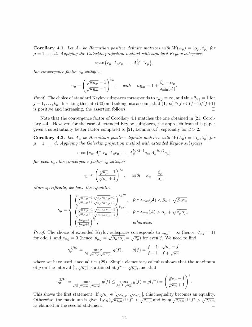
Corollary 4.1. Let Aµ be Hermitian positive definite matrices with W (Aµ) = [αµ, βµ] forµ = 1, . . . , d. Applying the Galerkin projection method with standard Krylov subspaces

span{cµ, Aµcµ, . . . , A

kµ−1µ cµ

},

the convergence factor γµ satisfies

γµ =

(√κR,µ − 1√κR,µ + 1

)kµ, with κR,µ = 1 +

βµ − αµλmin(A)

.

Proof. The choice of standard Krylov subspaces corresponds to zµ,j ≡ ∞, and thus θµ,j = 1 forj = 1, . . . , kµ. Inserting this into (30) and taking into account that (1,∞) 3 f 7→ (f−1)/(f+1)is positive and increasing, the assertion follows.

Note that the convergence factor of Corollary 4.1 matches the one obtained in [21, Corol-lary 4.4]. However, for the case of extended Krylov subspaces, the approach from this papergives a substantially better factor compared to [21, Lemma 6.1], especially for d > 2.

Corollary 4.2. Let Aµ be Hermitian positive definite matrices with W (Aµ) = [αµ, βµ] forµ = 1, . . . , d. Applying the Galerkin projection method with extended Krylov subspaces

span{cµ, A−1µ cµ, Aµcµ, . . . , A

kµ/2−1µ cµ, A

−kµ/2µ cµ}

for even kµ, the convergence factor γµ satisfies

γµ ≤

(4√κµ − 1

4√κµ + 1

)kµ, with κµ =

βµαµ.

More specifically, we have the equalities

γµ =

(√κL,µ−1√κL,µ+1

√κµ/κL,µ−1√κµ/κL,µ+1

)kµ/2, for λmax(A) < βµ +

√βµαµ,(√

κR,µ−1√κR,µ+1

√κµ/κR,µ−1√κµ/κR,µ+1

)kµ/2, for λmin(A) > αµ +

√βµαµ,(

4√κµ−1

4√κµ+1

)kµ, otherwise.

Proof. The choice of extended Krylov subspaces corresponds to zµ,j = ∞ (hence, θµ,j = 1)for odd j, and zµ,j = 0 (hence, θµ,j =

√βµ/αµ =

√κµ) for even j. We need to find

γ2/kµµ = max

f∈[√κL,µ,

√κR,µ]

g(f), g(f) =f − 1

f + 1·√κµ − f

f +√κµ.

where we have used inequalities (29). Simple elementary calculus shows that the maximumof g on the interval [1,

√κµ] is attained at f∗ = 4

√κµ, and that

γ2/kµµ = max

f∈[√κL,µ,

√κR,µ]

g(f) ≤ maxf∈[1,

√κµ]g(f) = g(f∗) =

(4√κµ − 1

4√κµ + 1

)2

.

This shows the first statement. If 4√κµ ∈ [

√κL,µ,

√κR,µ], this inequality becomes an equality.

Otherwise, the maximum is given by g(√κL,µ) if f∗ <

√κL,µ and by g(

√κR,µ) if f∗ >

√κR,µ,

as claimed in the second statement.

12

Finally, we get the following bound for a rational Krylov subspace method with two shifts,∞ and σ ∈ R \W (Aµ), the latter possibly depending on µ. This is a generalization ofextended Krylov subspaces, where σ = 0, and we will see that it allows for faster convergence,while requiring the same number of linear system solves in the method.

Corollary 4.3. Let Aµ be Hermitian positive definite matrices with W (Aµ) = [αµ, βµ] forµ = 1, . . . , d. Applying the Galerkin projection method with rational Krylov subspaces of theform

span{cµ, (Aµ − σI)−1cµ, Aµcµ, . . . , Akµ/2−1µ cµ, (Aµ − σI)−kµ/2cµ}

for even kµ, the convergence factor γµ satisfies

γµ ≤ max

{(√θ − 1√θ + 1

)kµ,

(√κR,µ − 1√κR,µ + 1

·∣∣∣∣√κR,µ − θ√κR,µ + θ

∣∣∣∣)kµ/2}

, (31)

with θ =√

σ−βµσ−αµ and κR,µ = 1 +

βµ−αµλmin(A) .

The shift minimizing this bound is given by

σopt = αµ(θ2opt − κµ)/(θ2

opt − 1), (32)

with θopt := s−1(√κµ) for s(θ) :=

[(θ + 1)2 + (θ − 1)

√θ2 + 6θ + 1

]/(4√θ). When using this

shift σopt, we have

γµ ≤

(6√

4κR,µ − 16√

4κR,µ + 1

)kµ. (33)

Proof. The choice of rational Krylov subspaces corresponds to zµ,j =∞ (hence, θµ,j = 1) for

odd j, and zµ,j = σ (hence, θµ,j =√

σ−βµσ−αµ =: θ) for even j. We need to find

γ2/kµµ = max

f∈[√κL,µ,

√κR,µ]

gθ(f), gθ(f) =f − 1

f + 1·

∣∣∣∣∣f − θf + θ

∣∣∣∣∣.The function gθ(f) is continuously differentiable in all points except 1 and θ, see Figure 1. Ithas a unique local maximum at

√θ. Combined with (29), this shows the bound (31):

γ2/kµµ = max

f∈[√κL,µ,

√κR,µ]

gθ(f) ≤ maxf∈[1,

√κR,µ]

gθ(f) = max{gθ(√θ), gθ(

√κR,µ)

}.

To prove (32), we need to find θopt ∈ (0,∞) which minimizes the function h(θ) given by

h(θ) := max{gθ(√θ), gθ(

√κR,µ)

}= max{h1(θ), h2(θ)}

with h1(θ) :=(√θ − 1√

θ + 1

)2, h2(θ) :=

√κR,µ − 1√κR,µ + 1

∣∣∣√κR,µ − θ√κR,µ + θ

∣∣∣.The function h1(θ) is zero in 1, and monotonically increases with |θ−1|. Similarly, h2(θ) is zeroin√κR,µ, and monotonically increases with |θ−√κR,µ|. As both h1 and h2 are monotonously

decreasing on (0, 1], we clearly have θopt ≥ 1. Similarly, we find that θopt ≤√κR,µ. Therefore,

θopt is uniquely defined by the relation

h1(θopt) = h2(θopt), θopt ∈ [1,√κR,µ].

13

0 1 2 3 4 5 60

0.1

f

gθ(f

)

Figure 1: Function gθ(f) from the proof of Corollary 4.3 for θ = 4.

Inserting both functions leads to the condition√κR,µ = s(θopt), with the bijective function

s : [1,√κR,µ]→ [1, s(

√κR,µ)] defined in the statement of the corollary.

To show (33), it remains to prove

γ2/kµµ =

(√θopt − 1√θopt + 1

)2

≤

(6√

4κR,µ − 16√

4κR,µ + 1

)2

,

which is the case if and only if√θopt ≤ 6

√4κR,µ, or, equivalently, θ

3/2opt/2 ≤

√κR,µ = s(θopt).

This is easily seen from

2θ2 ≤ (θ + 1)2 + (θ − 1)2 ≤ (θ + 1)2 + (θ − 1)√θ2 + 6θ + 1, ∀q ≥ 0.

Remark 4.4. The convergence behavior tends to improve when d, the number of dimensions,increases. We illustrate this by considering the case Aµ ≡ A with W (A) = [α, β] and kµ ≡ k.Then the bound obtained from Corollary 4.1 for standard Krylov subspaces becomes

‖r‖2 ≤ 2√d ‖c‖2

√λmax(A)

λmin(A)

(√κR − 1√κR + 1

)k,

with κR = 1 + β−αdα < κ = β/α. Clearly, the effective condition number κR decreases as d

increases. A similar statement holds for the bound obtained from Corollary 4.3 for rationalKrylov subspaces with shifts∞ and σopt. However, for the case of extended Krylov subspaces,the bound generally only improves if the condition λmin(A) > αµ +

√βµαµ holds, that is, if√

κ < d− 1. Since it is unlikely that such a condition is satisfied, it follows that choosing anoptimal shift is essential for achieving improved results in higher dimensions.

Remark 4.5. For different but similar Blaschke-type rational functions, the quantity γkof (30) has been determined in [3, Section 6] for various configurations of poles, includingthose discussed in this section. If it is affordable to solve shifted systems with Aµ for severaldifferent shifts, one could imagine to choose zµ,1 =∞ and then cyclic shifts

zµ,2 = σ1, zµ,3 = σ2, . . . , zµ,p+1 = σp,zµ,p+2 = σ1, zµ,p+3 = σ2, . . . , zµ,2p+1 = σp,

. . .

14

for some fixed p. Note that σ1, . . . , σp will depend on µ. The so-called ADI optimal shifts areobtained by solving the third Zolotarev problem

minθµ,2,...,θµ,p+1

maxf∈[√κL,µ,

√κR,µ]

p+1∏j=2

∣∣∣∣∣f − θµ,jf + θµ,j

∣∣∣∣∣,see, e.g., [25, Sec. 2.1] and [11]. For instance, in the case p = 1 we get the convergence rate(√κR,µ/κL,µ − 1)/(

√κR,µ/κL,µ + 1) for the parameter θµ,2 =

√κR,µκL,µ.

5 Numerical Experiments

In this section, numerical experiments are presented to illustrate the theoretical results onthe convergence behavior obtained in Section 4 for Hermitian positive definite matrices.

Remark 5.1. The implementation of the Galerkin projection method requires the solutionof the linear system(

d∑µ=1

Ikd ⊗ · · · ⊗ Ikµ+1 ⊗ Aµ ⊗ Ikµ−1 ⊗ · · · ⊗ Ik1

)y = cd ⊗ · · · ⊗ c1,

at least once in the final step of the method. This system has size k1k2 · · · kd, which makes adirect approach infeasible for larger d, even when kµ � nµ. Instead, we use an approximatesolution based on exponential sums:

y =R∑j=1

ωj exp(−αjAd)cd ⊗ · · · ⊗ exp(−αjA1)c1,

see [14, 21]. The vector y is only stored implicitly through the vectors exp(−αjAµ)cµ. Thecoefficients αj , ωj , j = 1, . . . , R are chosen to approximate 1/ξ by the exponential sum∑R

j=1 ωje−αjξ [7, 15, 16]. As the approximation error decreases exponentially depending with

R, even moderate values of R lead to an accuracy at the level of about 10−8, which is usedin all experiments below.

Experiment 1: Standard Krylov subspaces. In the first example, we set all matricesAµ ≡ A, where A ∈ R200×200 is the standard finite difference discretization of the one-dimensional Laplace operator on [0, 1] with homogeneous Dirichlet boundary conditions. Theright-hand side is set to c = b⊗ b⊗ · · · ⊗ b, where the entries of b are random numbers fromN (0, 1) and b is normalized such that ‖b‖2 = 1. The obtained results are shown in the left plotof Figure 2. For d = 2, observed and predicted convergence rates match quite well. However,as d increases, the observed convergence becomes faster than predicted by Corollary 4.1. Thisphenomenon seems to depend strongly on the choice of b. To demonstrate this, let

b = UD−1e/‖UD−1e‖2, (34)

where A = UDUT is the eigenvalue decomposition of A and e = (1, . . . , 1)T . Then the resultsshown in the right plot of Figure 2 reveal that the observed and predicted convergence ratesmatch very well even for large d. Moreover, both the convergence rate does not improvevisibly as d increases, which confirms the observation made in Remark 4.4.

15

0 50 100 150 200

10−10

10−5

100

105

k

resid

ua

l n

orm

d = 2

d = 5

d = 10

d = 50

d = 100

0 50 100 150 200

10−10

10−5

100

105

k

resid

ua

l n

orm

d = 2

d = 5

d = 10

d = 50

d = 100

Figure 2: Norm of residuals for standard Krylov subspace method. Solid lines correspond tocomputed residuals and dashed lines correspond to the bound obtained from Corollary 4.1.Left: Randomly chosen right-hand side. Right: Particularly constructed right-hand side(34).

Experiment 2: Extended Krylov subspaces. We repeat Experiment 1 for extendedKrylov subspaces. The results for a random right-hand side are shown in the left plot ofFigure 3. Even for d = 2, the observed convergence is much faster than predicted by Corol-lary 4.2. Moreover, this phenomenon does not disappear with the right-hand side (34).

Inspired by a numerical experiment in [20, Example 4.2], we also consider a diagonalmatrix A ∈ Rn×n, n = 104, with diagonal elements

ajj =1

2√κ

((κ+ 1) + (κ− 1) cos

π(j − 1)

n− 1

), j = 1, . . . , n, (35)

where κ = 2500 = κ(A). The right-hand side vector is set to c = b ⊗ b ⊗ · · · ⊗ b, withb = A−1e. The obtained results are shown in the right plot of Figure 3. Again, the observedand predicted convergence rates match very well even for large d.

Experiment 3: Rational Krylov subspaces with shifts ∞ and σopt. We repeat Ex-periment 2 for rational Krylov subspaces with shifts∞ and σopt defined in Corollary 4.3. Theresults are displayed in Figure 4. The observed and predicted convergence rates match well.However, in contrast to Experiment 2, the convergence rates improve as d increases.

Experiment 4: Rational Krylov subspaces with optimal ADI shifts. In this ex-periment, we apply rational Krylov subspaces with optimal ADI shifts σ1, · · · , σp to thematrix (35) and the corresponding right-hand side. The obtained results for p = 1 and p = 3optimal ADI shifts are shown in the left and the right plot of Figure 5, respectively.

6 Conclusions

In this paper, we have provided an analysis of Galerkin projection onto tensor products ofsubspaces for linear systems that can be regarded as d-dimensional analogues of the Sylvester

16

0 50 100 150 200

10−10

10−5

100

105

k

resid

ua

l n

orm

d = 2

d = 5

d = 10

d = 50

d = 100

0 10 20 30 40 50 60

10−10

10−5

100

105

kre

sid

ual norm

d = 2

d = 5

d = 10

d = 50

d = 100

Figure 3: Norm of residuals for extended Krylov subspace method. Solid lines correspond tocomputed residuals and dashed lines correspond to the bound obtained from Corollary 4.2.Left: Discrete Laplace. Right: Diagonal matrix (35).

0 50 100 150 200

10−10

10−5

100

105

k

resid

ua

l n

orm

d = 2

d = 5

d = 10

d = 50

d = 100

0 10 20 30 40 50 60

10−10

10−5

100

105

k

resid

ual norm

d = 2

d = 5

d = 10

d = 50

d = 100

Figure 4: Norm of residuals for rational Krylov subspace method with shifts∞ and σopt. Solidlines correspond to computed residuals and dashed lines correspond to the bound obtainedfrom Corollary 4.3. Left: Discrete Laplace. Right: Diagonal matrix. (35).

17

0 10 20 30 40 50 60

10−10

10−5

100

105

k

resid

ual norm

d = 2

d = 5

d = 10

d = 50

d = 100

0 10 20 30 40 50 60

10−10

10−5

100

105

k

resid

ual norm

d = 2

d = 5

d = 10

d = 50

d = 100

Figure 5: Norm of residuals for rational Krylov subspace method with optimal ADI shifts.Solid lines correspond to computed residuals and dashed lines correspond to the bound fromTheorem 3.2. Left: One shift. Right: Three shifts.

equation. The orthogonal decomposition of the residual derived in Proposition 2.2 is thekey observation and allows to decompose the residual into a sum of residuals for simpler 1Dprojections, see Proposition 2.3. When applied to polynomial and rational Krylov subspaces,this decomposition allows to derive a priori error estimates via extremal problems for univari-ate rational functions. This contrasts with the analysis in [21], which involves multivariateapproximation problems. Numerical experiments demonstrate that the convergence rates de-rived in this paper are sharp. Moreover, our bounds allow for a better understanding of thedependence of the convergence rates on the shifts in the rational Krylov subspaces. In turn,this can be used to optimize the choice of shifts. Interestingly, the convergence of rationalKrylov subspace methods with optimized shifts improves as the dimension d increases.

References

[1] A. C. Antoulas. Approximation of Large-Scale Dynamical Systems. SIAM Publications,Philadelphia, PA, 2005.

[2] B. Beckermann. An error analysis for rational Galerkin projection applied to the Sylvesterequation. SIAM J. Numer. Anal., 49(6):2430–2450, 2011.

[3] B. Beckermann and L. Reichel. Error estimates and evaluation of matrix functions viathe Faber transform. SIAM J. Numer. Anal., 47(5):3849–3883, 2009.

[4] P. Benner and T. Breiten. Low rank methods for a class of generalized Lyapunovequations and related issues. Technical report, MPI Magdeburg, 2012. Available fromhttp://www.mpi-magdeburg.mpg.de/preprints/.

[5] P. Benner, R. Byers, E. S. Quintana-Ortı, and G. Quintana-Ortı. Solving algebraicRiccati equations on parallel computers using Newton’s method with exact line search.Parallel Comput., 26(10):1345–1368, 2000.

18

[6] P. Benner, R.-C. Li, and N. Truhar. On the ADI method for Sylvester equations. J.Comput. Appl. Math., 233(4):1035–1045, 2009.

[7] D. Braess and W. Hackbusch. Approximation of 1/x by exponential sums in [1,∞). IMAJ. Numer. Anal., 25(4):685–697, 2005.

[8] M. Crouzeix. Numerical range and functional calculus in hilbert space. J. Funct. Anal.,244(2):668–690, 2007.

[9] J. W. Demmel. Three methods for refining estimates of invariant subspaces. Computing,38:43–57, 1987.

[10] V. Druskin, L. Knizhnerman, and V. Simoncini. Analysis of the rational Krylov subspaceand ADI methods for solving the Lyapunov equation. SIAM J. Numer. Anal., 49(5):1875–1898, 2011.

[11] N. S. Ellner and E. L. Wachspress. Alternating direction implicit iteration for systemswith complex spectra. SIAM J. Numer. Anal., 28(3):859–870, 1991.

[12] O. G. Ernst. Minimal and orthogonal residual methods and their generalizations forsolving linear operator equations. Habilitation thesis, TU Bergakademie Freiberg, 2001.

[13] G. H. Golub and C. F. Van Loan. Matrix Computations. Johns Hopkins UniversityPress, Baltimore, MD, third edition, 1996.

[14] L. Grasedyck. Existence and computation of low Kronecker-rank approximations forlarge linear systems of tensor product structure. Computing, 72(3-4):247–265, 2004.

[15] W. Hackbusch. Approximation of 1/x by exponential sums. Available from http://

www.mis.mpg.de/scicomp/EXP_SUM/1_x/tabelle. Retrieved August 2008.

[16] W. Hackbusch. Entwicklungen nach Exponentialsummen. Technical Report, Max-Planck-Institut fur Mathematik in den Naturwissenschaften, 2009. Revised version. Seehttp://www.mis.mpg.de/preprints/tr/report-0405.pdf.

[17] I. M. Jaimoukha and E. M. Kasenally. Krylov subspace methods for solving large Lya-punov equations. SIAM J. Numer. Anal., 31:227–251, 1994.

[18] K. Jbilou. ADI preconditioned Krylov methods for large Lyapunov matrix equations.Linear Algebra Appl., 432(10):2473–2485, 2010.

[19] B. N. Khoromskij and Ch. Schwab. Tensor-structured Galerkin approximation of para-metric and stochastic elliptic PDEs. SIAM J. Sci. Comput., 33(1):364–385, 2011.

[20] L. Knizhnerman and V. Simoncini. Convergence analysis of the extended Krylov subspacemethod for the Lyapunov equation. Numer. Math., 118(3):567–586, 2011.

[21] D. Kressner and C. Tobler. Krylov subspace methods for linear systems with tensorproduct structure. SIAM J. Matrix Anal. Appl., 31(4):1688–1714, 2010.

[22] D. Kressner and C. Tobler. Preconditioned low-rank methods for high-dimensional ellip-tic PDE eigenvalue problems. Comput. Methods Appl. Math., 11(3):363–381, 2011.

19

[23] T. Mach and J. Saak. Towards an ADI iteration for tensor structured equations. Technicalreport, MPI Magdeburg, 2012. Available from www.mpi-magdeburg.mpg.de/preprints/

2011/12/.

[24] Y. Saad. Numerical solution of large Lyapunov equations. In Signal processing, scatteringand operator theory, and numerical methods (Amsterdam, 1989), volume 5 of Progr.Systems Control Theory, pages 503–511. Birkhauser Boston, Boston, MA, 1990.

[25] J. Sabino. Solution of Large-Scale Lyapunov Equations via the Block Modified SmithMethod. PhD thesis, Rice University, 2006.

[26] V. Simoncini. A new iterative method for solving large-scale Lyapunov matrix equations.SIAM J. Sci. Comput., 29(3):1268–1288, 2007.

[27] V. Simoncini and V. Druskin. Convergence analysis of projection methods for the nu-merical solution of large Lyapunov equations. SIAM J. Numer. Anal., 47:828–843, 2009.

[28] N. Truhar, Z. Tomljanovic, and R.-C. Li. Analysis of the solution of the Sylvesterequation using low-rank ADI with exact shifts. Systems Control Lett., 59(3-4):248–257,2010.

20