an epq model for multi level inv entory systems with ... · production inventory model for vendor...

An EPQ Model for Multi Level Inventory

Systems with Maximum Life for Deteriorating

Items and Exponential Credit Period Demand 1M. Ravithammal and

2P. Muniappan

1Department of Mathematics,

Vels University, Chennai,

Tamil Nadu, India.

[email protected] 2Department of Mathematics,

Sathyabama Institute of Science and Technology,

Chennai, Tamil Nadu, India.

[email protected]

Abstract In this paper production inventory model for items with a time varying

deterioration rate is studied and demand rate is supposed to be a positive

exponential function of credit period. In the inventory system shortages are

allowed and backlogged them partially. A manufacturer frequently offers

to his buyers a trade credit in order to stimulate sales and reduce inventory.

There is no interest charge to a buyer if the purchasing amount is paid to a

manufacturer within the credit period. On the other hand, granting a credit

period from a manufacturer to its buyer increases default risk. In this

paper, an EPQ model is proposed for a manufacturer when: (1)

deteriorating items not only deteriorate continuously, and has a maximum

lifetime, (2) credit period increases not only demand but also default risk,

and (3) inventory level considered for three stages, i.e., production, non

production and shortage period. A model is proposed to maximize the

profit function of inventory cycle. Numerical examples illustrate the

theoretical results.

Key Words:Inventory, exponential credit period, shortages, deteriorating

items.

International Journal of Pure and Applied MathematicsVolume 119 No. 10 2018, 1041-1052ISSN: 1311-8080 (printed version); ISSN: 1314-3395 (on-line version)url: http://www.ijpam.euSpecial Issue ijpam.eu

1041

International Journal of Pure and Applied Mathematics Special Issue

1042

1. Introduction

In reality, many products such as fruits, vegetables, high-tech products,

pharmaceuticals and volatile liquids not only deteriorate continuously due to

evaporation, obsolescence and spoilage but also have their expiration dates.

Atici et al. [1] studied inventory model of deteriorating items on non-periodic

discrete-time domains. Bhunia et al. [2] analyzed a two-warehouse inventory

model for deteriorating items under permissible delay in payment with partial

backlogging. Sarkar et al. [13] developed an inventory model with variable

demand, component cost and selling price for deteriorating items.

In the business world, stock-out situation plays an important role. Due to some

unavailable circumstances, stock-out situation may occur in any business.

According to the literature of inventory control theory, most of the inventory

models are developed under the assumption ‘‘shortages are allowed and

completely backlogged’’. In practice, this assumption is not realistic. Generally,

customers are not interested to wait for a long time to purchase goods from a

particular shop. Only a fraction of the customers waits to purchase the good

from a particular shop due to good behavior of the retailer, genuine price,

quality of the goods and also the locality of the shop. As a result, shortages are

considered as partially backlogged with a rate dependent on the length of

waiting time up to the arrival of fresh lot [2]. B. Sarkar and S. Sarkar [14]

developed an improved inventory model with partial backlogging, time varying

deterioration and stock-dependent demand. Chang and Dye [3] studied an EOQ

model for deteriorating items with time varying demand and partial

backlogging. Stojkovska [15] developed optimal policies for the deterministic

EPQ with partial backordering.

Chen and Teng [4] developed retailer’s optimal ordering policy for deteriorating

items with maximum lifetime under supplier’s trade credit financing.

Muniappan and Uthayakumar [6] developed a Mathematical technique for

computing optimal replenishment polices. Sarkar [12] studied an EOQ model

with delay in payments and time varying deterioration rate. Wang et al. [16]

developed seller’s optimal credit period and cycle time in a supply chain for

deteriorating items with maximum lifetime. Muniappan et al. [8] developed an

EOQ model for deteriorating items with inflation and time value of money

considering time-dependent deteriorating rate and delay payments.

Goyal and Giri [5] studied the production-inventory problem of a product with

time varying demand, production and deterioration rates. Muniappan et al. [7]

developed an economic lot sizing production model for deteriorating items

under two level trade credit. Ravithammal et al. [10] studied integrated

production inventory system for perishable items with fixed and linear

backorders. Ravithammal et al. [11] developed deterministic production

inventory model for buyer- manufacturer with quantity discount and completely


1043

backlogged shortages for fixed life time product. Muniappan et al. [9] studied

production inventory model for vendor–buyer coordination with quantity

discount, backordering and rework for fixed life time products.

Although numerous researchers have studied economic order quantity models

for deteriorating items, few of them have taken the maximum lifetime of a

deteriorating item into consideration. In this paper, an EPQ model is built for

the manufacturer to obtain profit function by incorporating the following

important and relevant facts: (1) deteriorating items not only deteriorate

continuously, and also has a maximum lifetime of the product (2) credit period

increases not only demand but also default risk, and (3) inventory level is

considered for three stages, i.e., production, non production and shortage period.

The remainder of this paper is organized as follows: Notations and Assumptions

are given in section 2. Model Formulation is presented in section 3. In Section

4, the numerical example is provided to illustrate the solution procedure.

Section 5 is concluded with remarks.

2. Notations and Assumptions

This study uses following notations and assumptions

Notations : Annual demand rate as a function of the credit period n

P : Annual production or replenishment rate must be greater than annual

demand rate P > D(n)

: The maximum lifetime in years for the deteriorating item

: The average production cost per unit per year in dollars

: Market price in dollars

r : The average ordering cost per order in dollars

h : The average stock holding cost per unit per year in dollars

s : The average shortage cost per unit per year in dollars

: The time varying deterioration rate at time t, where

: The inventory level that changes with time t during production periods

(units)

: The inventory level that changes with time t during non production periods

(units)

: The inventory level that changes with time t during shortage periods (units)

: The manufacturer’s optimal credit period in years

: The manufacturer’s optimal production cycle time in years

: The manufacturer’s optimal non production cycle time in years

: The manufacturer’s optimal cycle time in years

: The manufacturer’s profit function per year in dollars

Assumptions 1. The demand rate , is a positive exponential function of

credit period n, a and b are positive constants.


1044

2. Since the longer credit period to the buyer, the higher the default risk to the

manufacturer, it is assumed without loss of generality that the rate of

default risk giving the credit period n. It is followed the same assumption as

in Wang et al. [19], i.e., where k is constant.

3. All deteriorating items have their expiration rates. The physical

significance of deterioration rate is the rate to be close to 1 when the time is

approaching to the maximum life time . To make the problem tractable,

the same assumption is followed as in Sarkar [14] as well as in Chen and

Teng [6] that the deterioration rate is

4. Shortages are allowed and a fraction of demand is backlogged them

partially.

5. The backlogged rate is defined to be when inventory is negative,

where is backlogging parameter and it is a positive constant.

6. The replenishment cycle time T is less than or equal to because

3. Model Formulation

The manufacturer’s produces Q units at t = 0, a production run is started at time

t = 0. During production time, the inventory level gradually increases to a rate

. Subsequently, the inventory level reaches its maximum

at . Once, the maximum inventory is reached then the production is

ended. Obviously, the on hand inventory decreases due to demand and the time-

varying deterioration rate. In the proposed model, a cycle can be divided into

three periods. Here [0, ] is taken as production duration. During [ , ] is

taken as non production duration and [ ] is taken as a fraction of demand is

backlogged. Based on the above description the differential equation

representing the inventory status is given by,

(1)

With the boundary condition , we obtain

(2)

In the time interval [ , ] there is no production and the inventory level

declines due to both demand and tine – varying deterioration rates until

Therefore, the inventory level is described by the following differential equation

(3)

With the boundary condition , we obtained

(4)

Since the time interval [ ] is taken as a fraction of demand which is

backlogged, the inventory level described by the following differential equation


1045

(5)

Therefore, it is obtained that

(6)

The manufacturer production quantity is

(7)

The manufacturer’s annual profit function consists of the following components

1. Average ordering cost is

2. Average stock holding cost is

1 2( ) ℎ − 1+ − − −(1+ ) 1+ − 1+ − 21+ − 11+ − 1− 2 (8)

3. Average shortage cost is

(9)

4. Annual production cost is

(10)

5. Average annual revenue after default risk is

(11)

Hence, the manufacturer’s annual profit per unit time is given by

Total annual revenue after default risk- annual holding cost -

annual production cost - annual shortage cost - annual ordering cost

1 1+ + 1+ ( − 1) 1+ ( − 1)−( − 1)+1+ − 1 1+ 1+− −ℎ +(1+ ) 1+ − 1+ + (1+ − ) ℎ +(1+ ) 1+

− 1+ − 1 1+ 1+ − (12)

Solution Procedure

Now, by solving the following equations simultaneously we obtain the optimal

values to maximize the seller’s total profit.


1046

, , , (13)

provided they satisfy the sufficient conditions ,

, , .

Equation (13) is equivalent to

1 1+ + 1+ ( − 1) 1+ ( − 1)−( − 1)+1+ − 1 1+ 1+− −ℎ +(1+ ) 1+ − 1+ =0 (14)

and

1=0 (15)

and

1)+ =0 (16)

(17)

where

( − 1)−( − 1)+1+ − 1 1+ 1+ − −ℎ +(1+ ) 1+ − 1+ and ∆2= 1+ − ℎ 1+1+ 1+ − 1+ − 1+ 1+ −

From Equations (14), (15), (16) and (17), we can obtained the optimal values

.


1047

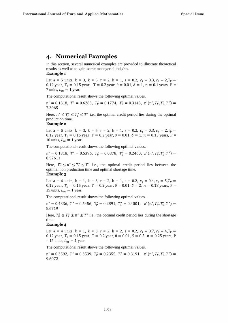
4. Numerical Examples

In this section, several numerical examples are provided to illustrate theoretical

results as well as to gain some managerial insights.

Example 1

Let a = 5 units, b = 3, k = 5, r = 2, h = 1, s = 0.2, , ,

, , , , , years, P =

7 units, year.

The computational result shows the following optimal values.

, , , ,

Here, i.e., the optimal credit period lies during the optimal

production time.

Example 2

Let a = 6 units, b = 3, k = 5, r = 2, h = 1, s = 0.2, , ,

, , , , , years, P =

10 units, year.


, , , ,

Here, i.e., the optimal credit period lies between the

optimal non production time and optimal shortage time.

Example 3

Let a = 4 units, b = 1, k = 3, r = 2, h = 1, s = 0.2, , ,

, , , , , years, P =

15 units, year.


, , , ,

Here, i.e., the optimal credit period lies during the shortage

time.

Example 4

Let a = 4 units, b = 1, k = 3, r = 2, h = 2, s = 0.2, , ,

, , , , , years, P

= 15 units, year.


, , , ,


1048

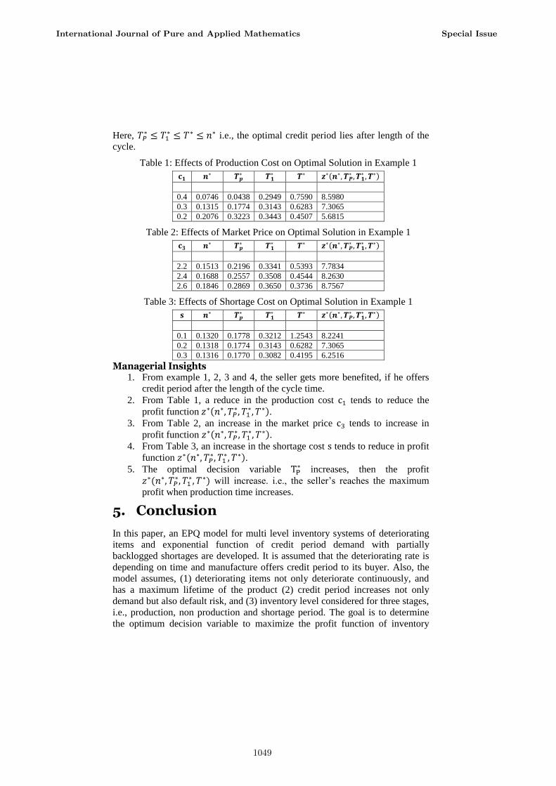
Here, i.e., the optimal credit period lies after length of the

cycle.

Table 1: Effects of Production Cost on Optimal Solution in Example 1

0.4 0.0746 0.0438 0.2949 0.7590 8.5980

0.3 0.1315 0.1774 0.3143 0.6283 7.3065

0.2 0.2076 0.3223 0.3443 0.4507 5.6815

Table 2: Effects of Market Price on Optimal Solution in Example 1

2.2 0.1513 0.2196 0.3341 0.5393 7.7834

2.4 0.1688 0.2557 0.3508 0.4544 8.2630

2.6 0.1846 0.2869 0.3650 0.3736 8.7567

Table 3: Effects of Shortage Cost on Optimal Solution in Example 1

0.1 0.1320 0.1778 0.3212 1.2543 8.2241

0.2 0.1318 0.1774 0.3143 0.6282 7.3065

0.3 0.1316 0.1770 0.3082 0.4195 6.2516

Managerial Insights 1. From example 1, 2, 3 and 4, the seller gets more benefited, if he offers

credit period after the length of the cycle time.

2. From Table 1, a reduce in the production cost tends to reduce the

profit function .

3. From Table 2, an increase in the market price tends to increase in

profit function .

4. From Table 3, an increase in the shortage cost tends to reduce in profit

function .

5. The optimal decision variable increases, then the profit

will increase. i.e., the seller’s reaches the maximum

profit when production time increases.

5. Conclusion

In this paper, an EPQ model for multi level inventory systems of deteriorating

items and exponential function of credit period demand with partially

backlogged shortages are developed. It is assumed that the deteriorating rate is

depending on time and manufacture offers credit period to its buyer. Also, the

model assumes, (1) deteriorating items not only deteriorate continuously, and

has a maximum lifetime of the product (2) credit period increases not only

demand but also default risk, and (3) inventory level considered for three stages,

i.e., production, non production and shortage period. The goal is to determine

the optimum decision variable to maximize the profit function of inventory


1049

cycle. It is observed that the optimal decision variables are highly impact on

maximum profit. Numerical example is performed to study the changes of the

decision variables and maximum profit. In future work it is proposed that after

considering single or two level trade credit policy, quantity discount rate etc.,

References

[1] Atici F.M., Lebedinsky A., Uysal F., Inventory model of deteriorating items on non-periodic discrete-time domains, European Journal of Operational Research 230 (2013), 284–289.

[2] Bhunia A.K., Chandra K.J., Anuj Sharma, Ritu Sharma, A two-warehouse inventory model for deteriorating items under permissible delay in payment with partial backlogging, Applied Mathematics and Computation 232 (2014), 1125–1137.

[3] Chang H.J., Dye C.Y., An EOQ model for deteriorating items with time varying demand and partial backlogging, Journal of the Operational Research Society 50 (1999), 1176-1182.

[4] Chen S.C., Teng J.T., Retailer’s optimal ordering policy for deteriorating items with maximum lifetime under supplier’s trade credit financing, Applied Mathematical Modelling 38 (2014), 4049-4061.

[5] Goyal S.K., Giri B.C., The production-inventory problem of a product with time varying demand, production and deterioration rates, European Journal of Operational Research 147 (2003), 549–557.

[6] Muniappan P., Uthayakumar R., Mathematical analyze technique for computing optimal replenishment polices, International Journal of Mathematical Analysis 8 (2014), 2979–2985.

[7] Muniappan P., Uthayakumar R., Ganesh S., An economic lot sizing production model for deteriorating items under two level trade credit, Applied Mathematical Sciences 8 (2014), 4737–4747.

[8] Muniappan P., Uthayakumar R., Ganesh S., An EOQ model for deteriorating items with inflation and time value of money considering time-dependent deteriorating rate and delay payments, Systems Science & Control Engineering 3 (2015), 427–434.

[9] Muniappan P., Uthayakumar R., Ganesh S., A production inventory model for vendor–buyer coordination with quantity discount, backordering and rework for fixed life time products,


1050

Journal of Industrial and Production Engineering 33 (2016), 355–362.

[10] Ravithammal M., Uthayakumar R., Ganesh S., An integrated production inventory system for perishable items with fixed and linear backorders, Int. Journal of Math. Analysis 8 (2014), 1549 – 1559.

[11] Ravithammal M., Uthayakumar R., Ganesh S., A deterministic production inventory model for buyer- manufacturer with quantity discount and completely backlogged shortages for fixed life time product, Global Journal of Pure and Applied Mathematics 11 (2015), 3583-3600.

[12] Sarkar B., An EOQ model with delay in payments and time varying deterioration rate, Mathematical and Computer Modelling 55 (2012), 367–377.

[13] Sarkar B., Saren S., Wee H.M., An inventory model with variable demand, component cost and selling price for deteriorating items, Economic Modelling 30 (2013), 306–310.

[14] Sarkar B., Sarkar S., An improved inventory model with partial backlogging, time varying deterioration and stock-dependent demand, Economic Modelling 30 (2013), 924-932.

[15] Stojkovska I., On the optimality of the optimal policies for the deterministic EPQ with partial backordering, Omega 41 (2013), 919-923.

[16] Wan-Chih Wang, Jinn-Tsair Teng, Kuo-Ren Lou, Seller’s optimal credit period and cycle time in a supply chain for deteriorating items with maximum lifetime, European Journal of operational Research 232 (2014), 315–321.


1051

an epq model for multi level inv entory systems with ... · production inventory model for vendor...

Documents