an enrollment retention study using a … · an enrollment retention study using a ... introduction...

AN ENROLLMENT RETENTION STUDY USING A MARKOV MODEL

FOR A REGIONAL STATE UNIVERSITY CAMPUS IN TRANSITION

Polly Wainwright Department of Mathematical Sciences

Department of Computer and Informational Sciences Indiana University, South Bend

E-mail Address: [email protected] November 16, 2007

Thesis submitted to the faculty of the University Graduate School in partial fulfillment of the requirements

for the degree of

Masters of Science

in

Applied Mathematics and Computer Science

Advisor

Dr. Yi Cheng Department of Mathematical Sciences

Committee

Dr. Yu Song

Dr. Dana Vrajitoru

ii

© 2007 Polly Wainwright

All Rights Reserved

iii

Table of Contents 1. Introduction 1 2. Literature Review 2 2.1 Retention Rates 2 2.2 Enrollment Retention Models 3 3. Purpose of Project 4 4. Development of Model 5 4.1 Transition and Initial State Matrices 6 4.2 Application of Markov Process 9 4.3 The Steady-State Matrix 10 5. Technology 13 6. Data, Assumptions, and Sorting 14 6.1 Sorting Criteria 16 6.2 Assumptions and Anomalies 22 6.2.1 Assumptions about Non-enrollment 22 6.2.2 Assumptions about New Students 22 6.2.3 Continuing But Not Continuous 23 6.2.4 Anomalies in Movement 25 7. Descriptive Statistics 26 8. First year Retention 29 9. Application of the Model to the Data 31 9.1 Initial State Matrix 31 9.2 Transition Matrix 33 9.3 The Six Year Graduation Rate 35 9.4 A Simpler Version of the Model 37

iv

10. Application of the Steady-State Model 42 10.1 The Steady-State Model Applied to Hours Enrolled 48 and Classification Index 10.2 The Steady-State Model Applied to Age 53 and Classification Index 10.3 The Steady-State Matrix Applied to Degree Groupings 58 10.4 Steady-State by Degree without Bridge Students 62 11. Summary and Analysis of Results 63 11.1 First-Year Retention 63 11.2 Graduation Rates 64 12. For Further Consideration 65 13. References 67

v

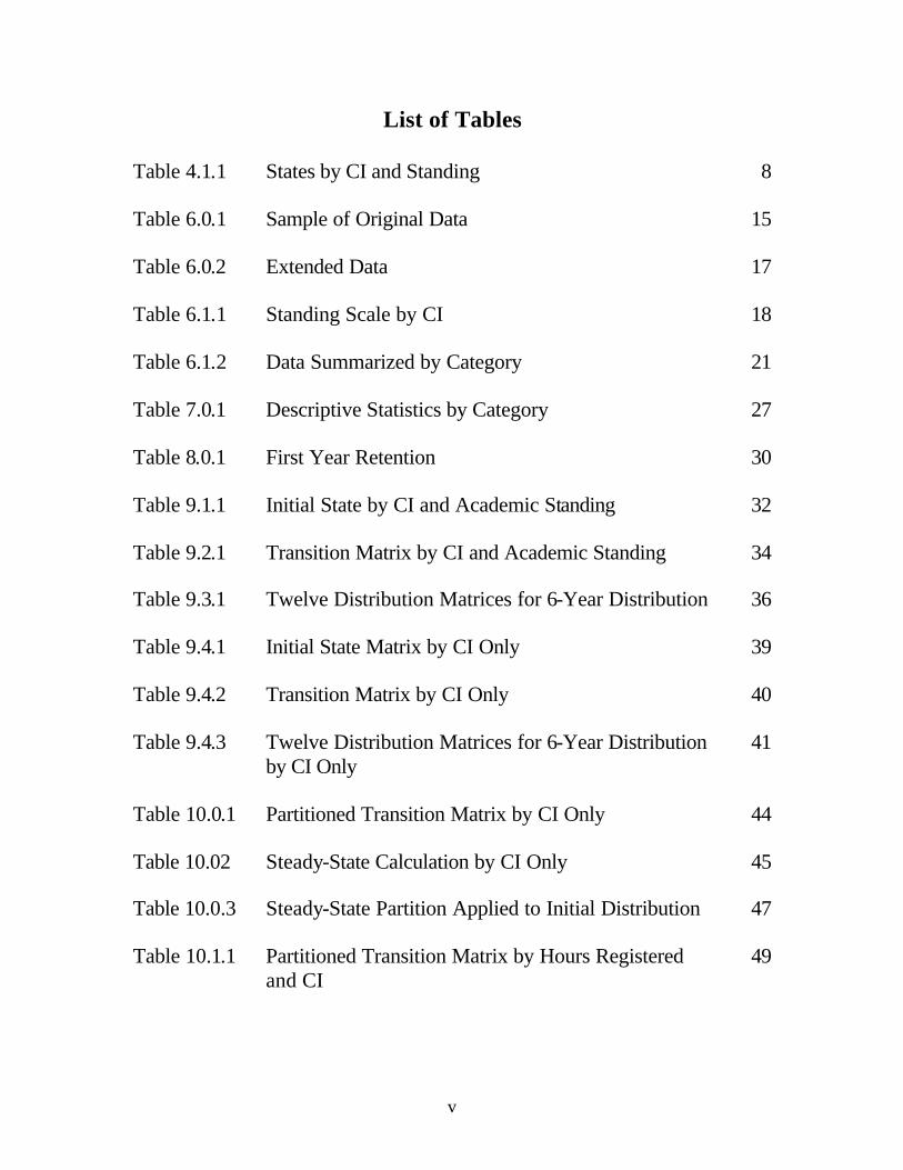
List of Tables

Table 4.1.1 States by CI and Standing 8 Table 6.0.1 Sample of Original Data 15 Table 6.0.2 Extended Data 17 Table 6.1.1 Standing Scale by CI 18 Table 6.1.2 Data Summarized by Category 21 Table 7.0.1 Descriptive Statistics by Category 27 Table 8.0.1 First Year Retention 30 Table 9.1.1 Initial State by CI and Academic Standing 32 Table 9.2.1 Transition Matrix by CI and Academic Standing 34 Table 9.3.1 Twelve Distribution Matrices for 6-Year Distribution 36 Table 9.4.1 Initial State Matrix by CI Only 39 Table 9.4.2 Transition Matrix by CI Only 40 Table 9.4.3 Twelve Distribution Matrices for 6-Year Distribution 41 by CI Only Table 10.0.1 Partitioned Transition Matrix by CI Only 44 Table 10.02 Steady-State Calculation by CI Only 45 Table 10.0.3 Steady-State Partition Applied to Initial Distribution 47 Table 10.1.1 Partitioned Transition Matrix by Hours Registered 49 and CI

vi

Table 10.1.2 Steady-State Calculation by Hours Registered 50 and CI Table 10.1.3 Steady-State Partition Applied to Initial Distribution 53 Table 10.2.1 Partitioned Transition Matrix by Age and CI 54 Table 10.2.2 Steady-State Calculation by Ag and CI 55 Table 10.2.3 Steady-State Partition Applied to Initial Distribution 58 Table 10.3.1 Partitioned Transition Matrix by Degree Grouping 59 Table 10.3.2 Steady-State Calculation by Degree Grouping 60 Table 10.3.3 Steady-State Partition Applied to Initial Distribution 61 Table 10.4.1 Steady-State Partition Applied to Initial Distribution 63 without Bridge Students

1

1. Introduction

Enrollment retention rates are an accepted indicator of a university’s success in

providing quality degree programs and learning environments which will lead to a

student’s continued enrollment and timely graduation from the university campus.

This project will analyze enrollment data from five consecutive years from a state

university regional campus, and construct an enrollment retention model using a Markov

process. Due to the agreement of confidentiality, the name of the campus will not be

revealed.

The model will be used to analyze enrollment retention rates for commonly

overlooked segments of the student population, as well as the retention rates for specific

degree programs, rather than just the retention rates for aggregate incoming freshmen.

This additional information will provide an opportunity for enrollment retention

committees to focus on improvement for all classifications of students, rather than just

the commonly observed freshmen, who are not necessarily representative.

The university from which the data has been collected is a regional campus of a

state university which has, over the past 40 years, transitioned from an off-campus site, to

a two-year community college, and recently, to an autonomous four-year-degree granting

institution with graduate programs in planning and student housing under construction.

Retention figures tend to be used for comparison against national averages, and

against rates of local, as well as similar peer institutions.

This project seeks to compare various retention rates within the schools of this

campus for the purpose of gaining greater insight into areas where retention might be

improved.

2

2. Literature Review 2.1 Retention Rates

There are two types of commonly accepted retention rates: the freshman-to-

sophomore retention rate, and the six-year retention rate.

The freshman-to-sophomore retention rate is based on the number of first semester

freshmen enrolling in a fall semester who then enroll as sophomores the following fall at

the same campus. This retention rate is widely accepted as the key retention figure since

students are most likely to drop out during their freshman year. The assumption is that

students who progress to their sophomore year are less at risk for dropping out, and will

likely go on to graduate from that campus.

The six-year retention rate is based on the number of first semester freshmen

enrolling in a fall semester who go on to graduate from that campus, with a four-year

degree, within a six year period. This retention rate seeks to measure timely graduation.

In both instances, the retention rates apply only to full- time freshmen seeking a four-year

degree.

Retention literature stresses that students who attend full-time and do not have

outside employment have 70-75% graduation rate, nationally. Students who attend only

part-time or who work full-time have an approximately 50% graduation rate. Further,

only about 50% of students graduate from the institution where they began as freshmen.

Of students whose college experience includes campus transfers, fewer than 10%

progress to graduation. (Dworkin, 2005)

Retention rates are of interest not only to universities hopeful of maintaining or

increasing enrollment, but act as a socio-economic indicator of well-being for the

3

community as a whole. It is, therefore, considered to be in the best public interest to

maintain high retention rates.

2.2 Enrollment Retention Models

Markov processes, regression models, and cohort flow models are three common

techniques used for enrollment prediction. While all three methods are appropriate for

the data available, the Markov model allows for a convenient table for viewing multiple

states.

The Markov model makes use of readily available cross-sectional historical

enrollment data and can be initiated at any point for which the data is available.

(Armacost and Wilson, 2002)

Markov models tend, however, to comprise a small number of states derived from

aggregate student populations, specifically all students in all degree programs, or

freshmen in all degree programs, rather than more specifically defined student

classifications. (Kraft and Jarvis, 2005)

Further, Markov models have specifically appropriate uses. The Markov model

assumes no trend in data, that the probability of flow from one state to the next will

remain consistent for the life for the model. Yet, the university environment naturally

evolves with changes to and additions of degree programs, changing student populations,

and the growth of distance learning options. (UCF, 2005) The Markov model is best

reserved for projections of no more than 10 years.

4

3. Purpose of the Project

The retention rate definitions described above apply to full- time first semester

freshmen enrolling in a fall semester, and only apply to those students pursuing a four-

year degree.

A preliminary analysis of the data for the campus being studied indicates that at

least one-third of the students are registered for 9 or few credit hours, with one-half of the

students registered for fewer than 12 credit hours.

Slightly fewer than 25% of new students at this campus are first-time freshmen.

About 10% of students are non-degree seeking students. This means that about 65% of

the newly enrolled students are transfer students who are not represented in typical

retention rate analysis.

Fewer than 30% of students are in a four-year degree program.

Finally, about half of all enrolled students are over the age of 25, with the average

student age being approximately 29. Students over the age of 25 are classified as non-

traditional or adult students. While available data does not include employment status, it

would be reasonable to assume that many adults are employed at least part-time.

Regional campuses in general, and this campus, specifically, do not have the same

student demographics as main campuses. Clearly, the normally accepted retention rate

descriptions summarized in the previous section do not adequately account for the student

demographics at this university campus. Therefore, a new model, using a Markov

process, will be used to analyze available enrollment data with respect to appropriate

rather than commonly accepted student classifications.

5

The one-year freshman-to-sophomore retention rate can be expanded for all student

classifications, specifically the transfer students that comprise 65% of new students at

this campus. Therefore, one-year retention rates will be determined for all classifications

of students, as well as for traditional and non-traditional age groupings.

Similarly, a six-year retention model will be constructed for all students using a

Markov process. Finally, a steady-state matrix will be developed in order to project the

long-term graduation rate for students in more relevant groupings.

4. Development of Model

The Markov model is based on an underlying stochastic process in which a system

in one state, si, moves to a subsequent state, sj. The states are commonly referred to as

the Current state and the Next state. The act of moving from one state to the next is

referred to as a step or transition.

The states are taken from a finite set of possible states { }nsssS ,,, 21 K= with each

transition from a state si to a state sj being defined by a transition probability jip of

occurring, and ∑=

=n

jjip

1

1 for i=1, . . . , n.

When the conditional probability of the Next state occurring, given the Current state

and the sequence of state preceding it, is dependent only on the Current state, or

independent of states previous to the Current state, the process is said to have the

memorylessness, or Markov Property.

( ) ( )immjmimmiiijm sXsXPsXsXsXsXsXP ======== ++ |,,,| 12211001 K , where mx

is the current state, 1+mx is the next state, and nimii ≤≤ ,1,01 .

6

A stochastic process with the Markov Property can be called a Markov Process or

Markov Chain.

For the retention model, the transition probabilities, ijp , will be obtained from the

relative frequencies of students in semester number, or Classification Index i moving to

Classification Index j in the period of one semester. Since only the Classification Index

of the Current semester, and the Classification Index of the Next semester will be noted,

the probability of moving from any Current state or semester to any Next state or

semester will be independent of states previous to the Current state. This independence

from previous states meets the criteria for the Markov Property, so this model can be

justifiably called a Markov Process.

4.1 Transition and Initial State Matrices

The Markov Process relies on two matrices: a transition matrix, and an initial state

matrix.

The transition matrix is an n-by-n matrix containing the transition probabilities, ijp ,

for moving from the Current state in the process to the Next state. In this model, the

Current states will be indicated by the matrix columns, and the Next states by the matrix

rows. For the transition matrix T, each cell contains the following transition probability:

[ ]ijjiji sspa |Pr== where j indicates the row, or Next state, and i indicates the column, or Current state, and

nji ≤≤ ,1 .

The following is a simplified version of the transition matrix for this model.

7

Current State Freshman Sophomore Junior Senior Freshman p11 p12 p13 p14 T = Next State Sophomore p21 p22 p23 p24 Junior p31 p32 p33 p34 Senior p41 p42 p43 p44

The purpose of the transition matrix is to represent the probability of movement

between states in a single time period. In this case, with what probability does a student

achieve a particular Classification Index by the end of the Current semester?

The possible states into which a student could be classified are determined by the

logical sorting criteria described below. The most basic states will include Classification

Index (semester number), academic standing, and assumptions regarding non-enrollment.

A student may become non-enrolled through graduation, by being academically

dropped by the university, or by leaving the university voluntarily without graduating

(Lost.)

Initially, there will be 10 classification indexes, 2 levels of academic standing, and

3 reasons for leaving the university. All reasonable combinations of these factors will

produce 23 individual states into which student data may be grouped, thus, necessitating

a 23-by-23 transition matrix. The Table 4.1.1 lists these states and provides a description

of each.

8

Table 4.1.1 States by CI and Standing

STATE DESCRIPTION

ND G non-degree seeking, good academic standing ND P non-degree seeking, academic probation FF G first semester freshman, good academic standing FF P first semester freshman, academic probation 1 G 1 - 15 credit hours, good academic standing 1 P 1 - 15 credit hours, academic probation 2 G 16 - 30 credit hours, good academic standing 2 P 16 - 30 credit hours, academic probation 3 G 31 - 45 credit hours, good academic standing 3 P 31 - 45 credit hours, academic probation 4 G 46 - 60 credit hours, good academic standing 4 P 46 - 60 credit hours, academic probation 5 G 61 - 75 credit hours, good academic standing 5 P 61 - 75 credit hours, academic probation 6 G 76 - 90 credit hours, good academic standing 6 P 76 - 90 credit hours, academic probation 7 G 91 - 105 credit hours, good academic standing 7 P 91 - 105 credit hours, academic probation 8 G 106+ credit hours, good academic standing 8 P 106+ credit hours, academic probation X D no longer enrolled, academically dropped X GR no longer enrolled, graduated X L no longer enrolled, lost

The data for students who are enrolled in the second, but not the first, of two

consecutive semesters will be used to determine the initial state matrix.

Further sorting will be done by degree program, student age, and full- or part-time

status.

The initial state matrix for the retention model will be a column matrix with a row

for each state, or a 23-by-1 matrix. Each cell of the initial state matrix will contain the

probability that a newly enrolled student will be classified in this state.

9

4.2 Application of the Markov Process

A Markov process is performed through matrix multiplication of the initial state

matrix and the transition matrix, resulting in, for this application, a distribution of student

states after one semester. In order to obtain a distribution matrix after many semester

transitions, the transition matrix need only be applied the desired number of times.

Specifically, 10 XTX = , where T is the transition matrix, 0X is the initial state

matrix, and 1X is the resulting distribution matrix after one transition.

Since the memorylessness property has been shown to be applicable, subsequent

transitions, and subsequent distribution matrices can be obtained by using the previous

distribution matrix as the current initial state matrix.

01 TXX =

( ) 02

012 XTTXTTXX ===

( ) 03

02

23 XTXTTTXX ===

This process can be generalized to say that the distribution matrix, after m time

periods or transitions is given by

0XTX mm =

Since one objective of this model is to produce a six-year retention rate, the

transition matrix will be applied (2 semesters) x (6 years) = 12 times, or

012

12 XTX =

10

4.3 The Steady-State Matrix

The distribution matrix, 12X , detailed in the previous section will provide a

description of the student population as a whole after 12 semesters. For example, it

might show that an initial state matrix representing a set of students of whom 7% are

sophomores becomes, after 12 transitions, a distribution matrix of whom only 1% are

sophomores. What this distribution matrix cannot describe is what has become of the

original 7% of the students who were sophomores, or for that matter, what has become of

any other specific group of students. It can only give a new distribution of the entire

student population.

In order to discover longer term trends or graduation rates for specific groups of

students, the steady state matrix is used. A matrix, X, is determined to be a steady state

matrix if there is a transition matrix, T, such that XT = X.

The transition matrix, T, tends toward a fixed matrix, L, as the number of

transitions, m, becomes large. In other words, it converges as m becomes large.

mTL ≈ for large enough values of m. A Markov chain with this property is called

ergodic.

For the retention model, the steady-state matrix, L, will describe the long term

outcome for groups of students. Specifically, given enough time, students must either

graduate, or leave the university, voluntarily or involuntarily. The steady-state matrix

will give the probabilities for those outcomes by group. Since the steady-state matrix

represents a long term trend, which may not actually be achieved in the university setting,

in this context, it can be thought of as a “best case” scenario for current student

demographics and movement.

11

The derivation of the steady-state matrix depends on the classification of the

transition matrix. In this case, the transition matrix is an absorbing matrix. An absorbing

stochastic matrix has the following properties:

1. There is at least one absorbing state, a state that once achieved is impossible to leave.

2. It is possible to move from any non-absorbing state to an absorbing state in one or

more transitions.

There are three absorbing states in the retention transition matrix. These three

states are the three conditions under which a student is no longer enrolled in the

university, dropped, graduated, or lost. (Since only Current and Next enrollment periods

are being considered, students who re-enroll after becoming non-enrolled are considered

to be new students. This topic will be dealt with in more detail below.)

To further meet the criteria for classification as an absorbing Markov matrix, it can

be shown, both from the transition matrix, and intuitively, that any absorbing state, any

reason for leaving the university, can be reached from any other non-absorbing state or

series of non-absorbing states. In other words, any student in any state can eventually

graduate, become academically dropped, or become “lost.”

In order to develop the steady-state matrix for the absorbing Markov matrix, the

transition matrix is required to be partitioned as follows:

12

CURRENT Absorbing Nonabsorbing

Absorbing I S NEXT

Nonabsorbing 0 R

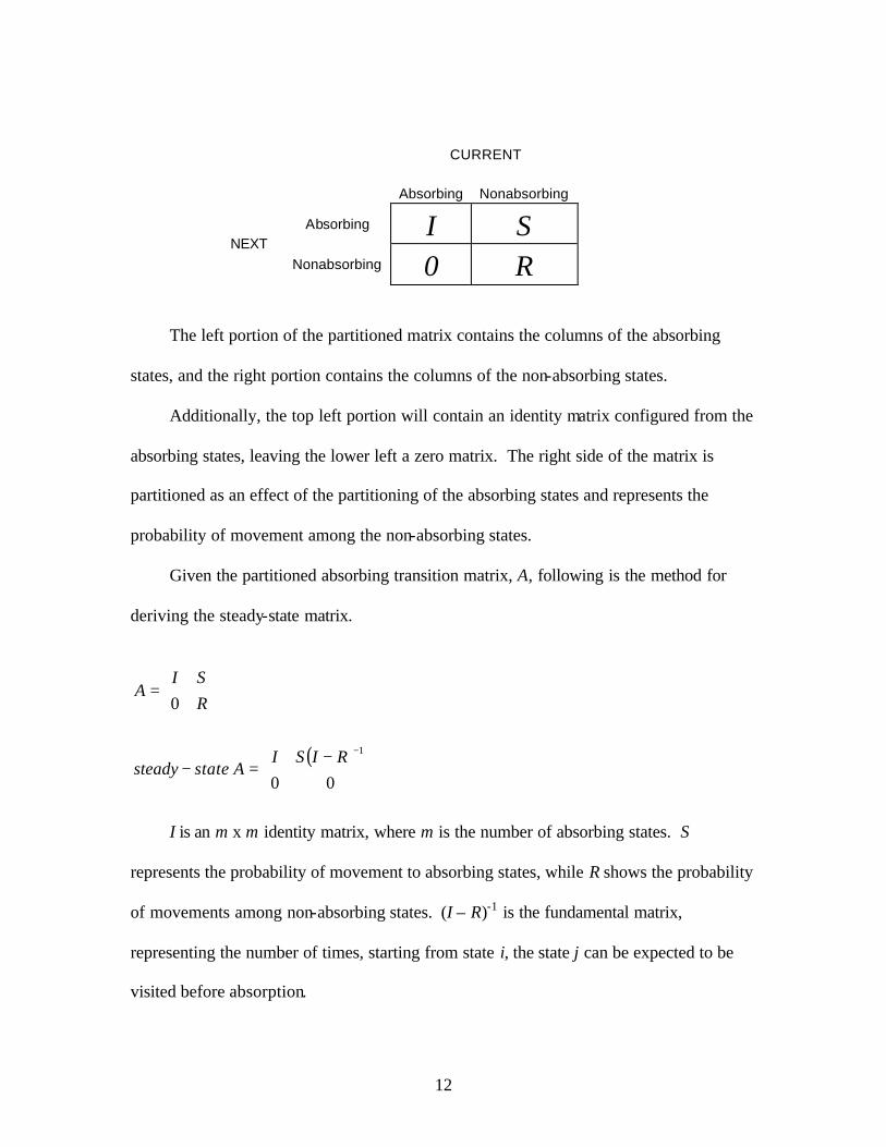
The left portion of the partitioned matrix contains the columns of the absorbing

states, and the right portion contains the columns of the non-absorbing states.

Additionally, the top left portion will contain an identity matrix configured from the

absorbing states, leaving the lower left a zero matrix. The right side of the matrix is

partitioned as an effect of the partitioning of the absorbing states and represents the

probability of movement among the non-absorbing states.

Given the partitioned absorbing transition matrix, A, following is the method for

deriving the steady-state matrix.

=

RSI

A0

( )

−=−

−

00

1RISIAstatesteady

I is an m x m identity matrix, where m is the number of absorbing states. S

represents the probability of movement to absorbing states, while R shows the probability

of movements among non-absorbing states. (I – R)-1 is the fundamental matrix,

representing the number of times, starting from state i, the state j can be expected to be

visited before absorption.

13

5. Technology

The data were made available from the campus registrar in the form of Excel

spreadsheets. Sorting is done using the standard Excel sorting function.

The transitioning of the Markov model is done in Excel using the matrix

multiplication function, mmult(array1, array2).

This function is a tool for finding the ordinary matrix product of two arrays. The

arrays may be, and in this case are, two-dimensional arrays, or matrices.

The product of m-by-n Matrix A and n-by-p Matrix B will be placed in m-by-p

Matrix C. Each element in Matrix C will be calculated as follows:

∑=

+++==•=n

knjinjijikjikkjikij babababaBAC

12211 K

where mi ≤≤1 and pj ≤≤1 .

The Excel function mmult(MatrixA, MatrixB) is applied to each cell in the defined

range for the destination Matrix C.

The calculation of the steady-state matrix is also done in Excel. In addition to using

the mmult(array1, array2) function, it also requires the matrix inverse function

minverse(array) where array is a square matrix.

The inverse of a matrix, A, is calculated by first joining it with an identity matrix of

the same dimension to form the augmented matrix

[ ]IA | which is then reduced, if possible, to the form [ ]BI | using Gauss-Jordan elimination. The matrix B is then the inverse of A, and AB=I.

14

6. Data, Assumptions, and Sorting

The 10 most recent consecutive semesters’ enrollment data (Fall 2000 - Spring

2005) were obtained from the university campus being studied. The complete set of data

consisted of approximately 32,000 data points. Each data point contains data pertinent to

an individual student’s enrollment for a particular semester. The data used for sorting

and determining states includes an anonymous student identification key, classification

by credit hours earned, cumulative grade point average (GPA), number of hours

registered, date of birth, and major code. Each data point does not represent a unique

student. Several data points will represent a single student’s enrollment over several

semesters.

Data are included for all students enrolled in the given semesters. The data is a

census, not a sample.

Only undergraduate student data are considered for this model. Graduate student

data, as well as data for students earning post-baccalaureate certificates and endorsements

were eliminated. This data set was identified using the degree code for each data point.

Also eliminated were data points for approximately 600 incoming students who had

cumulative GPAs of 0.0. A GPA of 0.0 can be the result of a student’s enrolling but then

withdrawing before the end of the semester, by never attending and receiving an

“unearned F,” or by receiving a legitimate grade of F. No direct information in the data

indicates the reason for the 0.0 GPA. Therefore, all such data points were eliminated

based on the assumption that these data points likely represented withdrawals, but with

the recognition that some legitimate data points might have been eliminated as well.

These data points represented less that 2% of the total data points, but nearly 10% of

15

incoming students. Their inclusion would have made the first year retention rates

artificially low.

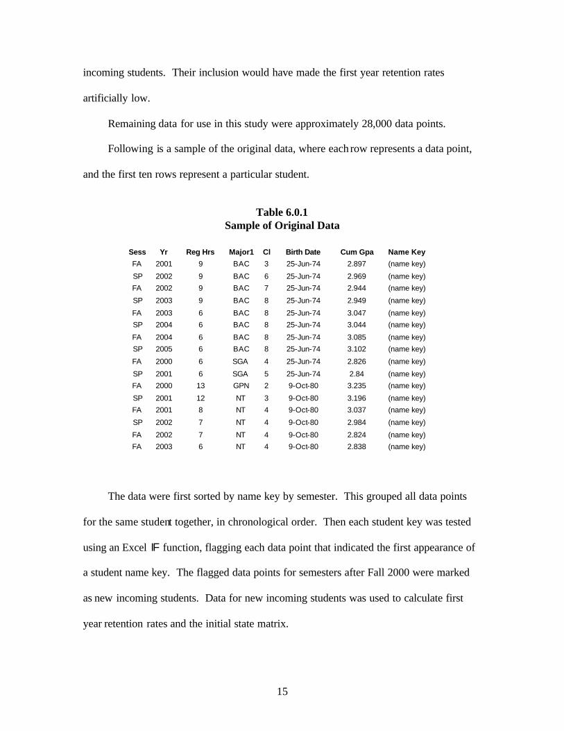
Remaining data for use in this study were approximately 28,000 data points.

Following is a sample of the original data, where each row represents a data point,

and the first ten rows represent a particular student.

Table 6.0.1

Sample of Original Data

Sess Yr Reg Hrs Major1 Cl Birth Date Cum Gpa Name Key

FA 2001 9 BAC 3 25-Jun-74 2.897 (name key)

SP 2002 9 BAC 6 25-Jun-74 2.969 (name key)







FA 2000 6 SGA 4 25-Jun-74 2.826 (name key)

SP 2001 6 SGA 5 25-Jun-74 2.84 (name key)

FA 2000 13 GPN 2 9-Oct-80 3.235 (name key)

SP 2001 12 NT 3 9-Oct-80 3.196 (name key)

FA 2001 8 NT 4 9-Oct-80 3.037 (name key)

SP 2002 7 NT 4 9-Oct-80 2.984 (name key)

FA 2002 7 NT 4 9-Oct-80 2.824 (name key)

FA 2003 6 NT 4 9-Oct-80 2.838 (name key)

The data were first sorted by name key by semester. This grouped all data points

for the same student together, in chronological order. Then each student key was tested

using an Excel IF function, flagging each data point that indicated the first appearance of

a student name key. The flagged data points for semesters after Fall 2000 were marked

as new incoming students. Data for new incoming students was used to calculate first

year retention rates and the initial state matrix.

16

Each data point includes data for the Current semester. Each data point needed to

be extended to include data for the Next semester as well. Since the data was

chronologically sorted, the Next semester data point was on the line below. This second

line was appended to the line above it using a simple Excel macro that copied the second

line, and pasted it to cells at the end of the first line. The flagging mentioned above acted

as a stopping mechanism for the macro in order to prevent two different students’ data

from being erroneously combined.

At this time, major codes were also used to include columns for major, school, and

type of degree.

A sample of the extended data points follows in Table 6.0.2.

6.1 Sorting Criteria

Student data was sorted by Classification Index, levels 1 through 8, which is

determined by number of credit hours earned. A Classification Index of 1 indicates 1 to

15 credit hours earned, and is commonly thought of as first semester freshman; a

Classification Index of 2 indicates 15 to 30 credit hours earned for a second semester

freshman, and so forth. Special classifications include FF for first-time freshmen and ND

for non-degree seeking students.

Data will also be sorted by cumulative GPA in order to further group students by

academic standing. Students will be determined to be in good academic standing or on

academic probation based on the criteria in the university’s student handbook.

Table 6.0.2

Extended Data

Name Key Sess Yr Reg Hrs Major1 Cl Birth Date Cum Gpa Standing Major School Degree Sess Yr Reg Hrs Major1 Cl Birth Date Cum Gpa Standing Major School Degree

1 (name key) FA 2003 12 PBS 1 17-Jun-85 2.333 G Pre-Behavioral Science General Studies Pre SP 2004 12 PBS 1 17-Jun-85 1.429 P Pre-Behavioral Science General Studies Pre

1 (name key) FA 2004 9 BPR FF 7-May-85 1.333 P Pre-General Business General Studies Pre SP 2005 12 BPR 1 7-May-85 0.857 P Pre-General Business General Studies Pre

1 (name key) FA 2000 6 GGG 1 30-Nov-71 2 G Bridge General Studies Bridge SP 2001 3 GGG 1 30-Nov-71 1 P Bridge General Studies Bridge

1 (name key) FA 2002 13 GLA 1 27-Mar-84 0 P Pre-Liberal Arts General Studies Pre SP 2003 12 GLA 1 27-Mar-84 0.6 P Pre-Liberal Arts General Studies Pre

1 (name key) FA 2002 12 GSE 1 12-Aug-83 1 P Pre-Education General Studies Pre SP 2003 12 GSE 1 12-Aug-83 1.4 P Pre-Education General Studies Pre

1 (name key) FA 2003 14 PAT 1 10-Jan-85 0.667 P Pre-Architectural Technology General Studies Pre SP 2004 12 PAT 1 10-Jan-85 1.333 P Pre-Architectural Technology General Studies Pre

1 (name key) FA 2003 10 ANO 1 26-Aug-84 0.3 P No Option Agriculture Transfer SP 2004 12 ANO 1 26-Aug-84 0.682 P No Option Agriculture Transfer

1 (name key) FA 2002 6 GPN 1 26-Apr-80 0 P Pre-Nursing General Studies Pre SP 2003 6 GPN 1 26-Apr-80 1 P Pre-Nursing General Studies Pre

(name key) SP 2003 6 GPN 1 26-Apr-80 1 P Pre-Nursing General Studies Pre FA 2003 6 PPN 1 26-Apr-80 0.333 P Pre-Nursing General Studies Pre

1 (name key) FA 2002 12 GSE 1 7-Dec-83 1 P Pre-Education General Studies Pre SP 2003 12 GSE 1 7-Dec-83 0.571 P Pre-Education General Studies Pre

1 (name key) FA 2001 9 GGG 1 17-Apr-82 0.667 P Bridge General Studies Bridge SP 2002 3 GGG 1 17-Apr-82 0.5 P Bridge General Studies Bridge

1 (name key) FA 2000 12 GGG 1 4-Apr-81 1 P Bridge General Studies Bridge SP 2001 12 GGG 1 4-Apr-81 0.2 P Bridge General Studies Bridge

1 (name key) FA 2003 9 UJC 1 8-Nov-81 2 G Journalistic Communications Liberal Arts Transfer SP 2004 12 UJC 1 8-Nov-81 1.286 P Journalistic Communications Liberal Arts Transfer

1 (name key) FA 2004 13 DGG FF 3-Jan-86 0 P Bridge General Studies Bridge SP 2005 13 DGG 1 3-Jan-86 0 P Bridge General Studies Bridge

(name key) FA 2000 13 GGG 1 17-Oct-64 1.3 P Bridge General Studies Bridge SP 2001 9 GGG 1 17-Oct-64 1.188 P Bridge General Studies Bridge

CURRENT NEXT

17

18

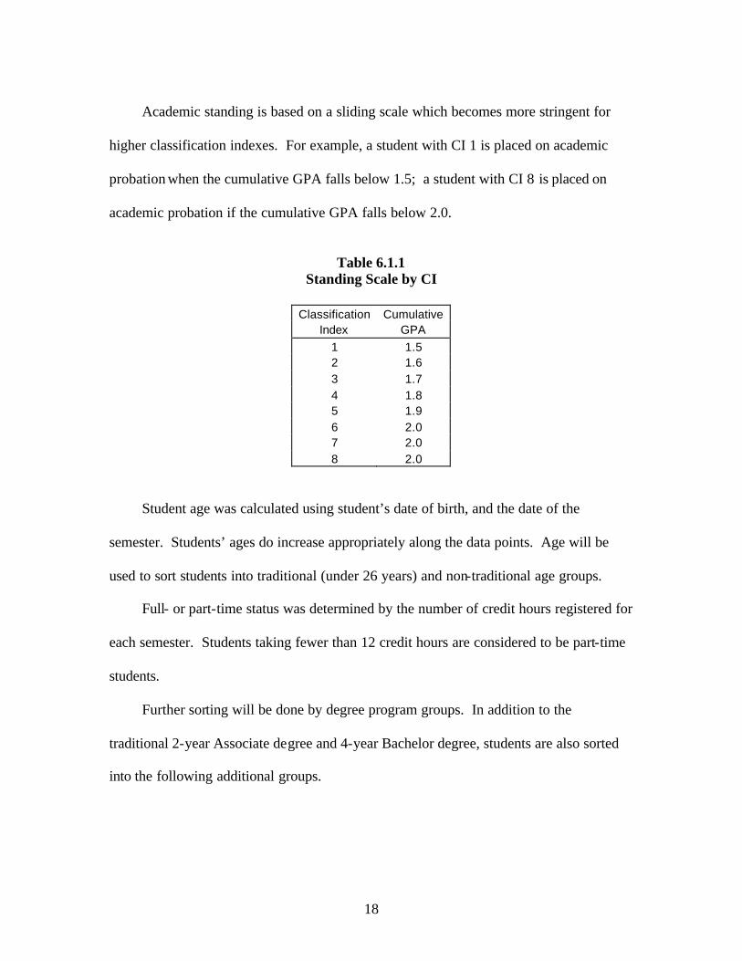
Academic standing is based on a sliding scale which becomes more stringent for

higher classification indexes. For example, a student with CI 1 is placed on academic

probation when the cumulative GPA falls below 1.5; a student with CI 8 is placed on

academic probation if the cumulative GPA falls below 2.0.

Table 6.1.1

Standing Scale by CI

Classification Cumulative Index GPA

1 1.5 2 1.6 3 1.7 4 1.8 5 1.9 6 2.0 7 2.0 8 2.0

Student age was calculated using student’s date of birth, and the date of the

semester. Students’ ages do increase appropriately along the data points. Age will be

used to sort students into traditional (under 26 years) and non-traditional age groups.

Full- or part-time status was determined by the number of credit hours registered for

each semester. Students taking fewer than 12 credit hours are considered to be part-time

students.

Further sorting will be done by degree program groups. In addition to the

traditional 2-year Associate degree and 4-year Bachelor degree, students are also sorted

into the following additional groups.

19

Bridge: A developmental program for students with deficiencies in their

educational backgrounds. There are specific standards that must be met before exiting

the bridge program.

High School: High achieving high school students who meet university entrance

requirements may take one course per semester while still in high school. This is an

option particularly attractive to home schooled high school students. The retention

committee would like to entice these highly motivated students to enroll as degree

seeking students, so their retention rates beyond high school is noteworthy.

Pre: Students who do not have university admission deficiencies, but are meeting

prerequisites for their majors are admitted to a Pre program. Requirements for

progressing from the Pre program to the major program varies greatly among degree

programs. For example, competitive programs, such as the nursing program, have higher

admission standards than university admissions, and a limited number of openings.

Students may never advance from the pre-nursing program. However, students in pre-

liberal studies, one of the biggest programs on the campus, just have to progress beyond

Classification Index 3. Later, it will be noted that the Pre group is the degree group that

contains the highest percentage of data points.

Transfer: Students who currently attend this campus but plan to transfer to a

different campus of the same university, or to a different university entirely are Transfer

students. Students planning to transfer are typically interested in a program not provided

at this campus, or are interested in a different university environment. They are treated

separately for retention rates, since they have no plan to graduate from this campus. It is

the hope of the retention committee to create programs and environments that might

20

attract these students to stay. Graduation rates from the campus under study will be noted

for students whose original plans were to transfer.

Undeclared: or Undecided is a catch-all group for many students, who, for example,

enroll during late admission and have no specific plans beyond enrolling, and students

who are visiting for a semester from other campuses. This category could also include

students who are taking courses after graduation from their degree program, but many of

those data points were likely flagged as graduate students and eliminated during the

initial sort of the data. The university discourages students from taking courses without a

degree objective.

A final preliminary sort groups data points into categories of CI, academic standing,

age, hours register, and degree group for both Current and Next semesters. The number

of data points in each of these very specific categories was tallied and used to summarize

each of the categories. A sample of the data points summarized by categories follows in

Table 6.1.2.

To interpret this summarized data, it can be noted from the first line that 62 full-

time, traditionally aged students in good academic standing in CI 1 seeking an Associate

degree were in exactly the same state the following semester. However, by reading line

2, it can be noted that 5 students who began in the state described above changed degree

programs in the Next semester to seek a Bachelor degree.

21

Table 6.1.2 Data Summarized by Category

CURRENT NEXT Cl Standing Age Reg Hrs Group Cl Standing Reg Hrs Group Freq

1 G T F Associates 1 G F Associates 62 1 G T F Associates 1 G F Bachelors 5 1 G T F Associates 1 G F Pre 3 1 G T F Associates 1 G F Transfer 3 1 P T P Pre 1 G P Associates 2 1 P T P Pre 1 G P Bachelors 2 1 P T P Pre 1 G P Bridge 6 1 P T P Pre 1 G P Pre 11 1 P T P Pre 1 G P Transfer 1 1 P T P Pre 1 G P Undeclared 1 2 G T F Associates 2 G F Associates 7 2 G T F Associates 2 G F Bachelors 9 2 G T F Associates 2 G F Bridge 2 2 G T F Associates 2 G F Pre 6 2 G T F Associates 2 G F Transfer 4 2 G T F Associates 2 G F Undeclared 3 2 P T F Pre 3 P F Pre 1 2 P T F Pre 3 P F Transfer 1 2 P T F Pre 3 P F Undeclared 1

22

6.2 Assumptions and Anomalies 6.2.1 Assumptions about Non-enrollment

Students who are enrolled in the first of two consecutive semesters but not the

second became non-enrolled because they had been academically dropped by the

university, graduated, transferred to another university, or stopped attending college

altogether. No direct information about these states is available in the data. Assumptions

are made based on Classification Index and academic standing.

Students in good academic standing with a CI of 8, and students in two-year degree

programs with a CI of 4 or higher were assumed to have graduated after the Current

semester.

Students who were on academic probation in the Current semester and non-enrolled

in the Next semester were considered to have been academically dropped by the

university.

No distinction could be made between students who transferred to other universities

and students who stopped attending college altogether. Students in good academic

standing but with CIs that were not near graduation in the Current semester were simply

given the classification (L)ost.

6.2.2 Assumptions about New Students

Students who were enrolled for the second of two consecutive semesters, but not

the first were considered to be newly enrolled students of any possible classification

index. This includes freshmen, transfers from other campuses, and non-degree seeking

students. These new students were simply given the appropriate classification index.

23

Students who might have attended this campus previous to the time period of the

data were still considered to be transfer students with previous college credits. No

distinction is made for re-admitted students.

Students who enrolled for one or more semesters, become non-enrolled for any

period of time, and then enroll again within the time period of the data were still

considered to be newly enrolled students upon re-enrollment. Commentary regarding this

phenomenon follows in the next section.

Students may be admitted to this campus with Unqualified Admission, Provisional

Admission, or Probationary Admission. No information is given in the data regarding

admission status. A backward assumption is therefore made that the admission status

was likely to be that same as the academic standing at the end of Current semester. New

students are, for this model, classified as Probationary or in Good Standing based on the

Current semester GPA.

An exception is made in the case of the Initial State matrix for first-time freshmen

(FF) and non-degree seeking students since it is university policy to accept such students

only in Good Standing. First-time freshmen and non-degree students will be classified

for the transition matrix as described above.

6.2.3 Continuing But Not Continuous Enrollment

While sorting data and classifying student states, it became apparent that students

commonly enroll for a number of semesters, drop out for a number of semesters, and then

re-enroll.

In keeping with the memorylessness property that is a requirement for a Markov

model, any enrollment status previous to the Current semester must be disregarded. As

24

such, re-enrollment could not be a consideration for this model. However, this pattern of

enrollment might cause the drop out rate to be artificially high if these continuing but not

continuous students do go on to graduate.

Distinct patterns of enrollment and non-enrollment, for example, the students who

enroll for consecutive Fall semesters, but none of the Spring semesters, do bring to mind

one of the most prominent characteristics of the student demographics that is not

quantified in this data. At the time that this data was gathered, all students commuted to

campus, and with rare exception, lived with family. Family and work/financial

obligations nearly universally affect enrollment patterns for individual students.

A method was sought, therefore, to consider the phenomenon of continuing but not

continuous enrollment, while maintaining the memorylessness property. This was

accomplished by reclassifying the data points with breaks in enrollment not as (L)ost, but

as (C)ontinuing. The data points for periods of enrollment were classified with the

normal CI, but were not additionally marked as newly enrolled students.

This procedure can be justified as memorylessness in the same way that academic

standing can be used as a classification even though it is a product of a cumulative GPA.

Academic standing and the classification of (C)ontinuing are still only dependent on the

previous semester’s movement.

Further restrictions could be placed on the classification of (C)ontinuing,

specifically, requiring enrollment after two consecutive semesters of (C)ontinuing, but

implementation of this classification demonstrated that none of this was necessary.

Reclassification of continuing but not continuous students revealed that less than

5% of data points previous classified as (L)ost, and fewer than 1% of all data points were

25

effected. Further, of the data points that were reclassified as (C)ontinuing, only about 5%

went on to have continuing enrollment. The remainder just went on to become (L)ost a

semester later.

The conclusion drawn from this necessary investigation was that students who

become non-enrolled and then re-enroll do not exist in high enough numbers to justify

special distinction in this model. Therefore, re-enrolled students will be classified as

newly enrolled transfer students, as described in the previous section.

6.2.4 Anomalies in Movement

It might seem reasonable that the logical transition for students from one semester

to the next would be either to remain in the Classification Index they were in, give or take

academic performance, or more to the next classification index.

It can observed in the Data Summarized by Category and later in the Transition

Matrix that movement can take the form of leaps over one or more indexes, or even move

in reverse.

In the first instance, the leap over classification indexes can be explained by transfer

credits that have been added during the semester, or credits received through test out. It

is the accumulation of credit hours that determines the Classification Index, so movement

need not be sequential.

Additionally, while there is no direct information obtained from the data, backward

movement in classification index can be explained by changes in major or transfers to

other schools within the campus. Such a change might result in loss of credit hours and

an apparent backward movement.

26

Also, in spite of specific guidelines for Classification Index assignment, the process

can still be subjective, and errors can occur. A new student’s initial Classification Index

is often a “best guess” based on information the student reports, which may not be

accurate. Further, the specific Classification Index label does not have an impact on a

student’s actual progress. An incorrect or out of date CI might not be caught and

corrected for several semesters. Unusual movement does not occur with enough

frequency to affect rates being calculated.

7. Descriptive Statistics

Values from the Data Summarized by Category is now used to calculate descriptive

statistics for the sorting categories of interest. These data are shown in Table 7.0.0.1.

An overview of the descriptive statistics for new students reveals that the new

admission Classification Index with the highest probability is Classification Index 1 at

62%. This is the group commonly referred to as the First Semester Freshman, but should

not be confused with Classification Index FF, the First Time Freshman. CI 1 freshmen

are those being admitted to the university with some previous college credits. In fact,

nearly 80% of new students is this data have previous college credits, with only 13% of

new students being First Time Freshmen (FF) and 8% being non-degree seeking students

(ND) whose histories are unknown.

27

Table 7.0.1 Descriptive Statistics by Category

Classification New All Index Students Students FF 661 13% 788 3% 1 3,225 62% 8,932 31% 2 337 6% 4,527 16% 3 147 3% 3,529 12% 4 219 4% 5,087 18% 5 64 1% 1,121 4% 6 47 1% 1,042 4% 7 23 0% 848 3% 8 103 2% 1,309 5% ND 397 8% 1,182 4%

TOTAL 5,223 28,365 Academic New All Standing Students Students Good Standing 4,817 92% 26,420 93% Probation 406 8% 1,945 7%

TOTAL 5,223 28,365 New All Age Students Students Traditional (under 26) 3,660 70% 18,378 65% Non-traditional 1,563 30% 9,987 35%

TOTAL 5,223 28,365 Hours New All Registered Students Students Full-time 2,666 51% 13,671 48% Part-time (under 12 cr hr) 2,557 49% 14,694 52%

TOTAL 5,223 28,365 Degree New All Grouping Students Students Associates 447 9% 5,100 18% Bachelors 952 18% 8,366 29% Bridge 701 13% 2,462 9% High School 131 3% 310 1% Pre 1,970 38% 8,475 30% Transfer 512 10% 2,224 8% Undeclared 510 10% 1,428 5%

TOTAL 5,223 28,365

28

The descriptive statistics for all students reveals that the majority of all students,

80%, are in Classification Indexes FF through 4, or freshmen and sophomores. Sixteen

percent of all students are upper level students in CI 5 through 8, with 4% of all students

being non-degree seeking. There is such a significant difference between the percentages

of lower level students with 12% to 31% in each Classification Index compared to 3% to

5% in upper level CIs that it might first appear that the community college environment

still exists, with the majority of students attending for only two years. However, it will

shortly be shown that the highest percentage of students is not for those seeking two-year

degrees.

A high percentage of both new and all students are in good academic standing (92%

and 93%.) Approximately half of both new and all students are part-time students.

Seventy percent of new students are traditionally aged college students, under 26

years. Slightly fewer, 65% of all students are traditionally aged. This is a higher

percentage than the initially stated projection that only half of the students were

traditionally aged.

The degree grouping with the highest probability of classification by new students

is the Pre program at 38%, with 30% of all students in the Pre program. A higher

percentage of new students, 18%, are admitted to a Bachelor program than an Associate

program, 9%. This remains consistent for all students, with 29% in a Bachelor program

and 18% in an Associate program, each gaining a higher percentage as students move

from Pre and Bridge programs. The higher percentage of students in Bachelor programs

than Associate programs refutes the notion that the higher percentage of students in lower

29

level Classification Indexes is due to choice of degree program and earlier graduation

from two-year programs.

8. First Year Retention

The Data Summarized by Category was further sorted to include only data points

for students who appeared in the second of two consecutive semesters. These data points

were marked as New Students. New Students were not just First Time Freshmen, CI FF,

or even First Semester Freshmen, CI 1, but any new student in any Classification Index.

Further, to be considered a New Student, the student may enroll for the first time in either

the Spring or Fall semester.

If a new student is enrolled one year after first enrollment, that data point is marked

as Retained. If the new student is not enrolled one year later, that data point is marked as

Lost.

An analysis of the first year retention rates reveals that less than half of all new

students, 46%, are retained to the following year. Of all students classified as First Time

Freshmen, CI FF, only 1% are retained. Of CI 1, First Semester Freshmen with previous

college credit, only 19% are retained. Much higher levels of retention are achieved by

CIs 2 through 8, second semester freshmen through graduating seniors, supporting the

assertion that incoming freshmen are more at risk for dropping out, but it should be noted

that the upper level students with higher retention rates are still new, incoming transfer

students. They are not students who have progressed passed incoming freshmen status at

this campus.

30

Table 8.0.1 First Year Retention

Retained Lost All Students 2,706 44% 3,474 56% Classification Index Retained Lost FF 6 1% 659 99% 1 436 19% 1,894 81% 2 1,385 91% 144 9% 3 437 82% 97 18% 4 221 65% 117 35% 5 44 51% 43 49% 6 45 58% 33 42% 7 27 57% 20 43% 8 47 76% 15 24% ND 58 11% 452 89% Academic Standing Retained Lost Good Standing 2,601 46% 3,003 54% Probation 105 18% 471 82% Age Retained Lost Traditional 1,664 41% 2,402 59% Non-traditional 1,042 49% 1,072 51% Hours Registered Retained Lost Full-time 1,414 49% 1,487 51% Part-time 1,292 39% 1,987 61% Degree Group Retained Lost Associates 490 72% 190 28% Bachelors 776 61% 494 39% Bridge 205 28% 535 72% High School 6 4% 128 96% Pre 859 40% 1,303 60% Transfer 235 40% 355 60% Undeclared 135 22% 469 78%

31

The categories of academic standing, age, and hours registered show a similar

retention pattern as the All Students category: slightly fewer than 50% of incoming

students are retained to the next year. Exceptions can be seen for students on academic

probation, of whom only 18% are retained, and for part-time students, of whom only 39%

are retained.

When analyzing first year retention by degree group, it can be shown that 72% of

students in Associate degree programs, and 61% of students in Bachelor degree programs

are retained. This contrasts significantly with Bridge students at 28% and Pre students at

40%. A possible explanation for this phenomenon is that new students able to be

admitted directly into a degree program are likely more capable students, in general.

Students planning to Transfer also have a 40% first year retention rate, while Bridge

students are retained at 28%. Undeclared students have a 22% retention rate, and High

School students, only a 4% retention rate. These lower retention rates for the less

established degree groupings are not surprising, but still have the effect of lowing the

retention rates for aggregate categories like Classification Index and Hours Registered

which do not distinguish between degree groups.

9. Application of the Model to the Data 9.1 Initial State Matrix

Data points for students who enrolled in the second of two consecutive semesters

but not the first were marked as newly enrolled students. The frequencies of these data

points by category were used to calculate probabilities for the initial state matrix. The

initial state matrix for data sorted by CI and academic standing follows.

32

Table 9.1.1 Initial State by CI and Academic Standing

X0 =

The initial state matrix by CI and academic standing shows that the greatest

percentage of incoming students are First Semester Freshmen in good standing. Note that

the initial state matrix contains probabilities of 0.0000 for Non-degree (ND) and First-

time Freshmen (FF) on academic probation as described above.

It should be noted that the non-enrolled states are also included in this initial state

matrix. It may seem counterintuitive to include such states; however, they must be

included in order for the initial state and the transition matrices to have compatible

dimensions.

ND G 0.0975 ND P 0.0000 FF G 0.1111 FF P 0.0000 1 G 0.5681 1 P 0.0533 2 G 0.0435 2 P 0.0039 3 G 0.0266 3 P 0.0015 4 G 0.0388 4 P 0.0024 5 G 0.0120 5 P 0.0010 6 G 0.0073 6 P 0.0008 7 G 0.0052 7 P 0.0002 8 G 0.0266 8 P 0.0002 X D 0.0000 X GR 0.0000 X L 0.0000

33

9.2 Transition Matrix

The frequencies obtained in the Data Summarized by category were further

condensed in order to produce the transition matrix by CI and academic standing, Table

9.2.0.1. For example, in the Data Summarized by category, there were 73 current

students of CI 1 in good standing who remained CI 1 students in good standing at the end

of the next semester. There were a total of 184 current CI 1 students in good standing, so

397.018473

→ is the probability of a current CI 1 student in good standing remaining a CI

1 student if good standing at the end of the next semester.

The transition matrix shows, for example, that a student in CI 1 in good academic

standing has a 0.3341 chance of, in the next semester, progressing to CI 2 while

remaining in good academic standing.

Further examination of the matrix reveals that there are apparently states that are

impossible to achieve, states for which there is a probability of 0.0000. For example, the

probability of progressing from CI 4 in probationary academic standing to CI 5 in either

good or probationary standing appears to be 0.000. Intuitively, it is certainly possible to

make the transition from CI 4 to CI 5, but based on this data, highly unlikely. Of the

28,000 data points used to create the transition matrix, there were either no data points

demonstrating this transition, or so few that the probability contains no significant digits,

to four decimal places.

Table 9.2.1 Transition Matrix by CI and Academic Standing

T =

ND ND FF FF 1 1 2 2 3 3 4 4 5 5 6 6 7 7 8 8 X X XG P G P G P G P G P G P G P G P G P G P D GR L

ND G 0.3856 0.0889 0 - 0.0005 - 0.0002 - - - - - - - - - - - - - - - -

ND P 0.0075 0.0222 0 - 0.0001 - - - - - - - - - - - - - - - - - -

FF G 0.0131 0 0 - - - - - - - - - - - - - - - - - - - -

FF P 0 0 0 - - - - - - - - - - - - - - - - - - - -

1 G 0.1251 0.0222 0.5183 0.1414 0.3970 0.1020 0.0081 0.0311 0.0047 - 0.0040 - 0.0072 0.0667 0.0068 - 0.0047 0.3333 0.0107 - - - -

1 P 0.0065 0 0.0384 0.2626 0.0220 0.2092 0.0002 0.0104 - - - 0.0143 - - - - - - - - - - -

2 G 0.0056 0 0.1728 - 0.3341 0.0077 0.4069 0.0363 0.0105 - 0.0032 - 0.0126 0.0667 0.0098 - 0.0012 - 0.0038 - - - -

2 P 0 0 0.0122 - 0.0096 0.0242 0.0070 0.1244 - - - - - - - - - - - - - - -

3 G 0 0.0222 0 - 0.0196 0.0013 0.3812 - 0.2811 0.0337 0.0111 - 0.0045 - 0.0098 - 0.0095 - 0.0031 - - - -

3 P 0 0 0 - - 0.0013 0.0061 0.0725 0.0058 0.1573 - - - - - - - - - - - - -

4 G 0.0009 0 0 - 0.0036 - 0.0318 - 0.4872 - 0.5294 0.1429 0.0325 0.0667 0.0254 0.1111 0.0213 - 0.0404 - - - -

4 P 0 0 0 - - - - 0.0052 0.0047 0.0674 0.0018 0.2000 - 0.0667 - - - - - - - - -

5 G 0.0009 0 0 - 0.0012 - 0.0024 - 0.0183 - 0.1423 - 0.2385 0.0667 0.0117 - 0.0071 - 0.0023 - - - -

5 P 0 0 0 - 0.0001 - - - - - 0.0006 - - 0.0667 - - - - - - - - -

6 G 0 0 0 - 0.0013 - 0.0026 - 0.0035 - 0.0374 - 0.4571 0.0667 0.2361 - 0.0095 - 0.0053 - - - -

6 P 0 0 0 - - - - - - - 0.0006 - 0.0036 - - 0.1667 - - - - - - -

7 G 0.0009 0 0 - 0.0003 - 0.0006 - 0.0009 - 0.0187 - 0.0560 - 0.4849 0.0556 0.2270 - 0.0069 - - - -

7 P 0.0000 0 0 - - - - - - - 0.0002 - - - - 0.0556 0.0024 - - - - - -

8 G 0.0009 0 0 - 0.0001 - 0.0004 - 0.0003 - 0.0175 - 0.0108 - 0.0634 - 0.5366 0.3333 0.4256 - - - -

8 P 0 0 0 - - - - - - - - - - - - - 0.0012 - - - - - -

X D 0 0.8444 0 0.5960 - 0.6543 0.0002 0.7202 - 0.7416 - 0.6429 - 0.5333 - 0.6111 - 0.3333 - 1.0000 1.0000 - -

X GR 0 0 0 - - - - - 0.0006 - 0.1183 - 0.0126 - 0.0049 - 0.0095 - 0.5019 - - 1.0000 -

X L 0.4528 0 0.2583 - 0.2106 - 0.1526 - 0.1826 - 0.1149 - 0.1644 - 0.1473 - 0.1702 - - - - - 1.0000

check 1.0000 1.0000 1.0000 1.0000 1.0000 1.0000 1.0000 1.0000 1.0000 1.0000 1.0000 1.0000 1.0000 1.0000 1.0000 1.0000 1.0000 1.0000 1.0000 1.0000 1.0000 1.0000 1.0000

CURRENT

NE

XT

34

35

Similarly, the transition matrix suggests that any student in CI 8 with probationary

standing would have a 100% probability of being academically dropped by the

university. Again, this is a phenomenon of very few data points for students in

probationary standing in CI 8. Those data points that do exist are all for students who

were, in fact, academically dropped.

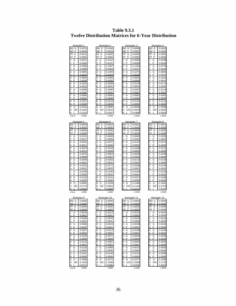
9.3 The Six-Year Graduation Rate

With the initial state matrix and transition matrix in place, the six-year graduation

rate can by calculated by transitioning the matrices as described above. Recall that in

order to move the initial state matrix through six years, the initial state matrix must be

multiplied twelve times by the transition matrix.

The following exhibit will show each of the twelve resulting matrices, with the

twelfth showing the final six-year distribution of students.

36

Table 9.3.1 Twelve Distribution Matrices for 6-Year Distribution

ND G 0.0379 ND G 0.0149 ND G 0.0059 ND G 0.0023ND P 0.0008 ND P 0.0003 ND P 0.0001 ND P 0.0001FF G 0.0013 FF G 0.0005 FF G 0.0002 FF G 0.0001FF P 0.0000 FF P 0.0000 FF P 0.0000 FF P 0.00001 G 0.3021 1 G 0.1311 1 G 0.0583 1 G 0.02681 P 0.0286 1 P 0.0131 1 P 0.0058 1 P 0.00262 G 0.2286 2 G 0.1957 2 G 0.1254 2 G 0.07242 P 0.0089 2 P 0.0063 2 P 0.0037 2 P 0.00203 G 0.0360 3 G 0.1040 3 G 0.1073 3 G 0.08043 P 0.0010 3 P 0.0024 3 P 0.0026 3 P 0.00214 G 0.0393 4 G 0.0483 4 G 0.0842 4 G 0.10244 P 0.0009 4 P 0.0005 4 P 0.0009 4 P 0.00105 G 0.0100 5 G 0.0098 5 G 0.0119 5 G 0.01745 P 0.0002 5 P 0.0001 5 P 0.0001 5 P 0.00016 G 0.0098 6 G 0.0096 6 G 0.0097 6 G 0.01186 P 0.0002 6 P 0.0001 6 P 0.0001 6 P 0.00017 G 0.0066 7 G 0.0080 7 G 0.0082 7 G 0.00917 P 0.0001 7 P 0.0000 7 P 0.0000 7 P 0.00008 G 0.0157 8 G 0.0118 8 G 0.0110 8 G 0.01148 P 0.0000 8 P 0.0000 8 P 0.0000 8 P 0.0000X D 0.0416 X D 0.0690 X D 0.0846 X D 0.0939X GR 0.0182 X GR 0.0310 X GR 0.0429 X GR 0.0587X L 0.2124 X L 0.3437 X L 0.4369 X L 0.5051check 1.0000 1.0000 1.0000 1.0000



Semester 1 Semester 2 Semester 3 Semester 4



37

Specifically, to obtain cell ij of matrix X1, the distribution matrix at the end of the

first semester, the following matrix algebra was used. T is the transition matrix, and X0 is

the initial state matrix.

( )( ) ( )( ) ( )( )

0379.0

0000.00000.00000.00889.00975.03865.023

1

1,02,021,01,0,0,1

=

+++=

+++==•=

∑

∑

=

=

k

n

knjinjijikjikkjikij xtxtxtxtXTX

K

K

The actual calculation was performed using the matrix multiplication function in

Excel: mmult(T, X0), where the matrix names are also defines range names. The

result of the calculation was placed in range X1. By analyzing the Semester 12

distribution matrix, it can be shown that, according to this model, 17.2% of the incoming

students had graduated within 6 years. Of these same incoming students, 68.23% had left

the university voluntarily without graduating, and 10.8% had been academically dropped.

These figures only account for 96.23% of the incoming students. The remaining

3.77% of the incoming students are still enrolled at the end of six years, in various states

of Classification Index and Academic Standing.

9.4 A Simpler Variation of the Model

The previous application of the model used states grouped by Classification Index

and Academic Standing, resulting in 23 individual states into which students could move.

However, in the final distribution matrix, Semester 12, the Academic Standing was

irrelevant since 96.23% of students had become non-enrolled.

38

In this next application of the model, the states will be grouped by Classification

Index alone, and Academic Standing will be omitted. This will reduce the number of

states through which students can transition to 13, and reducing the transition matrix by

almost half.

The next three exhibits will show the revised Initial State and Transition matrices,

and the new twelve semester distribut ions matrices. As before the twelfth semester

distribution matrix will show the final six-year distribution of students.

39

Table 9.4.1 Initial State Matrix by CI Only

Y0 = ND 0.0975

FF 0.1111 1 0.6214 2 0.0474 3 0.0282 4 0.0411 5 0.0130 6 0.0081 7 0.0054 8 0.0268 X D 0 X GR 0 X L 0

check 1.0000

Table 9.4.2 Transition Matrix by CI Only

T =

ND FF 1 2 3 4 5 6 7 8 X X XD GR L

ND 0.3817 - 0.0006 0.0002 - - - - - - - - - FF 0.0125 - - 0.0002 - - - - - - - - - 1 0.1272 0.5342 0.4090 0.0094 0.0045 0.0041 0.0080 0.0067 0.0059 0.0107 - - - 2 0.0054 0.1577 0.3150 0.4052 0.0102 0.0031 0.0134 0.0096 0.0012 0.0038 - - - 3 0.0009 - 0.0181 0.3765 0.2845 0.0110 0.0045 0.0096 0.0094 0.0030 - - - 4 0.0009 - 0.0033 0.0309 0.4812 0.5286 0.0339 0.0268 0.0212 0.0403 - - -

5 0.0009 - 0.0012 0.0023 0.0179 0.1410 0.2371 0.0115 0.0071 0.0023 - - - 6 - - 0.0012 0.0025 0.0034 0.0375 0.4554 0.2349 0.0094 0.0053 - - - 7 0.0009 - 0.0002 0.0005 0.0009 0.0186 0.0553 0.4784 0.2285 0.0068 - - -

8 0.0009 - 0.0001 0.0004 0.0003 0.0173 0.0107 0.0623 0.5371 0.4247 - - - X D 0.0341 0.0878 0.0602 0.0246 0.0187 0.0088 0.0071 0.0105 0.0012 0.0023 1.0000 - - X GR - - - - 0.0006 0.1167 0.0125 0.0048 0.0094 0.5008 - 1.0000 - X L 0.4346 0.2202 0.1913 0.1474 0.1780 0.1133 0.1622 0.1448 0.1696 - - - 1.0000

check 1.0000 1.0000 1.0000 1.0000 1.0000 1.0000 1.0000 1.0000 1.0000 1.0000 1.0000 1.0000 1.0000

CURRENTN

EX

T

40

41

Table 9.4.3 Twelve Distribution Matrices for 6-Year Distribution

by CI Only

ND 0.0376 ND 0.0146 ND 0.0057 ND 0.0022FF 0.0012 FF 0.0005 FF 0.0002 FF 0.00011 0.3272 1 0.1421 1 0.0631 1 0.02902 0.2338 2 0.1990 2 0.1271 2 0.07313 0.0379 3 0.1054 3 0.1083 3 0.08104 0.0407 4 0.0495 4 0.0848 4 0.10245 0.0105 5 0.0101 5 0.0121 5 0.01736 0.0105 6 0.0100 6 0.0100 6 0.01197 0.0071 7 0.0083 7 0.0085 7 0.00928 0.0158 8 0.0121 8 0.0114 8 0.0117X D 0.0528 X D 0.0809 X D 0.0975 X D 0.1077X GR 0.0185 X GR 0.0314 X GR 0.0436 X GR 0.0595X L 0.2065 X L 0.3359 X L 0.4278 X L 0.4948check 1.0000 1.0000 1.0000 1.0000



Semester 9

Semester 1 Semester 2 Semester 3


Semester 10 Semester 11 Semester 12

Semester 4

42

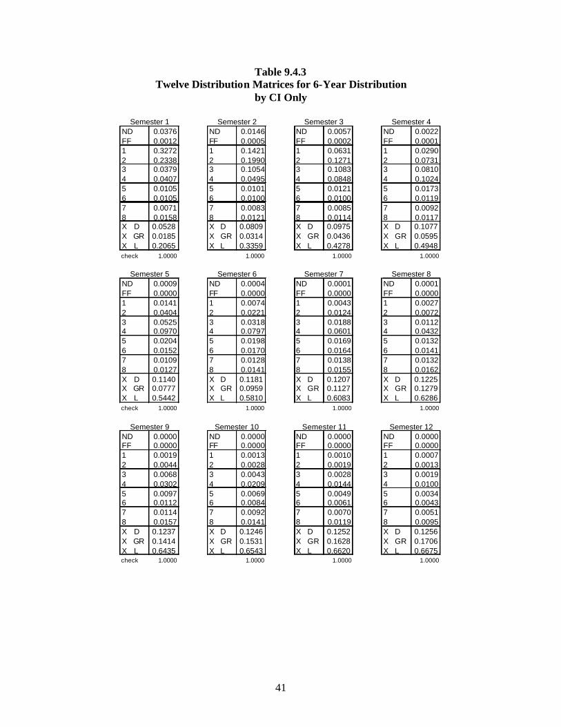
By analyzing the Semester 12 distribution matrix for the simplified CI Only model,

it can be shown that the final six-year distribution is very similar to the result obtained by

the CI and Academic Standing model.

According to this model, 17.06% of students had graduated within 6 years, 66.75%

of students had left the university voluntarily without graduating, and 12.56% had been

academically dropped by the university.

Again, this accounts for only 96.37% of the initial distribution of students. The

remaining 3.63% of students are still enrolled in various states of Classification Index.

The simpler version of the model yields virtually the same result. Therefore, this

would be the most appropriate version of the model to use since it would require less

sorting and a smaller model.

10. Application of the Steady-State Model

The steady-state model as described above will be applied to the data developed in

the last section. The steady-state model will use the same transition matrix as the CI

Only version of the model. An initial state matrix is not required for the steady-state

model.

First, the distribution matrix developed above will be partitioned into absorbing and

non-absorbing states. This is simple a rearrangement of rows and columns so that the

absorbing states form the upper left quadrant of the partitioned matrix. This partition is

an identity matrix, since the probability of remaining in an absorbing state is always 1.

The upper right quadrant contains the probabilities of moving from a non-absorbing state,

to an absorbing state. The lower right quadrant shows the probabilities of movement

among the non-absorbing states. The probabilities in the two right quadrants are the

43

same for correlating row and column headings in the transitions matrix, T. The lower

left quadrant shows the probability of movement from an absorbing state to a non-

absorbing state. Since this is impossible, the lower left quadrant is a zero matrix. The

complete partitioned transition matrix follows.

Additional exhibits will show the sequence of matrices that are required to develop

the steady state matrix.

Table 10.0.1 Partitioned Transition Matrix by CI Only

X X X ND FF 1 2 3 4 5 6 7 8D GR L

X D 1.0000 0 0 0.0341 0.0878 0.0602 0.0246 0.0187 0.0088 0.0071 0.0105 0.0012 0.0023X GR 0 1.0000 0 0 0 0 0 0.0006 0.1167 0.0125 0.0048 0.0094 0.5008X L 0 0 1.0000 0.4346 0.2202 0.1913 0.1474 0.1780 0.1133 0.1622 0.1448 0.1696 0

ND 0 0 0 0.3817 0 0.0006 0.0002 0 0 0 0 0 0FF 0 0 0 0.0125 0 0 0.0002 0 0 0 0 0 01 0 0 0 0.1272 0.5342 0.4090 0.0094 0.0045 0.0041 0.0080 0.0067 0.0059 0.01072 0 0 0 0.0054 0.1577 0.3150 0.4052 0.0102 0.0031 0.0134 0.0096 0.0012 0.00383 0 0 0 0.0009 0 0.0181 0.3765 0.2845 0.0110 0.0045 0.0096 0.0094 0.00304 0 0 0 0.0009 0 0.0033 0.0309 0.4812 0.5286 0.0339 0.0268 0.0212 0.04035 0 0 0 0.0009 0 0.0012 0.0023 0.0179 0.1410 0.2371 0.0115 0.0071 0.00236 0 0 0 0 0 0.0012 0.0025 0.0034 0.0375 0.4554 0.2349 0.0094 0.00537 0 0 0 0.0009 0 0.0002 0.0005 0.0009 0.0186 0.0553 0.4784 0.2285 0.00688 0 0 0 0.0009 0 0.0001 0.0004 0.0003 0.0173 0.0107 0.0623 0.5371 0.4247

check 1.0000 1.0000 1.0000 1.0000 1.0000 1.0000 1.0000 1.0000 1.0000 1.0000 1.0000 1.0000 1.0000

NE

XT

CURRENT

44

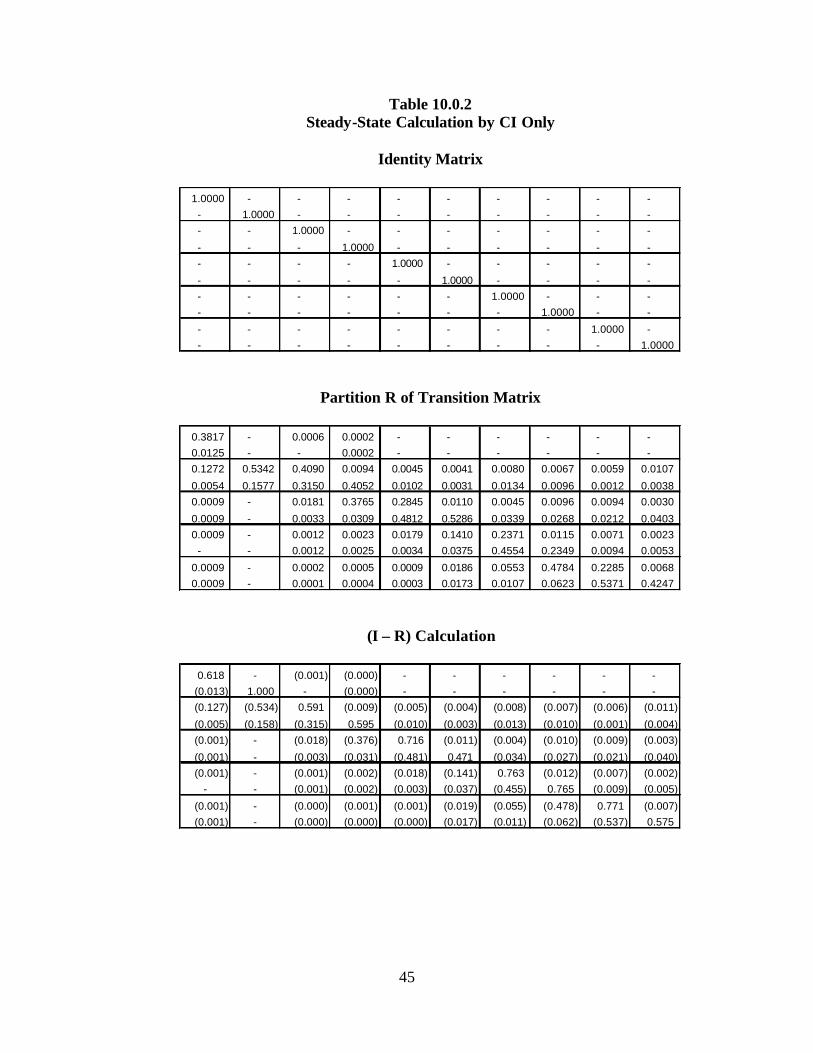
45

Table 10.0.2 Steady-State Calculation by CI Only

Identity Matrix

1.0000 - - - - - - - - -

- 1.0000 - - - - - - - - - - 1.0000 - - - - - - -

- - - 1.0000 - - - - - - - - - - 1.0000 - - - - -

- - - - - 1.0000 - - - - - - - - - - 1.0000 - - - - - - - - - - 1.0000 - -

- - - - - - - - 1.0000 - - - - - - - - - - 1.0000

Partition R of Transition Matrix

0.3817 - 0.0006 0.0002 - - - - - - 0.0125 - - 0.0002 - - - - - - 0.1272 0.5342 0.4090 0.0094 0.0045 0.0041 0.0080 0.0067 0.0059 0.0107

0.0054 0.1577 0.3150 0.4052 0.0102 0.0031 0.0134 0.0096 0.0012 0.0038 0.0009 - 0.0181 0.3765 0.2845 0.0110 0.0045 0.0096 0.0094 0.0030

0.0009 - 0.0033 0.0309 0.4812 0.5286 0.0339 0.0268 0.0212 0.0403 0.0009 - 0.0012 0.0023 0.0179 0.1410 0.2371 0.0115 0.0071 0.0023

- - 0.0012 0.0025 0.0034 0.0375 0.4554 0.2349 0.0094 0.0053

0.0009 - 0.0002 0.0005 0.0009 0.0186 0.0553 0.4784 0.2285 0.0068 0.0009 - 0.0001 0.0004 0.0003 0.0173 0.0107 0.0623 0.5371 0.4247

(I – R) Calculation

0.618 - (0.001) (0.000) - - - - - - (0.013) 1.000 - (0.000) - - - - - - (0.127) (0.534) 0.591 (0.009) (0.005) (0.004) (0.008) (0.007) (0.006) (0.011)

(0.005) (0.158) (0.315) 0.595 (0.010) (0.003) (0.013) (0.010) (0.001) (0.004) (0.001) - (0.018) (0.376) 0.716 (0.011) (0.004) (0.010) (0.009) (0.003)

(0.001) - (0.003) (0.031) (0.481) 0.471 (0.034) (0.027) (0.021) (0.040) (0.001) - (0.001) (0.002) (0.018) (0.141) 0.763 (0.012) (0.007) (0.002)

- - (0.001) (0.002) (0.003) (0.037) (0.455) 0.765 (0.009) (0.005)

(0.001) - (0.000) (0.001) (0.001) (0.019) (0.055) (0.478) 0.771 (0.007) (0.001) - (0.000) (0.000) (0.000) (0.017) (0.011) (0.062) (0.537) 0.575

46

Table 10.0.2 (continued) (I – R)-1 Inverse of (I – R) Matrix

1.6178 0.0011 0.0019 0.0006 0.0001 0.0001 0.0001 0.0001 0.0000 0.0000 0.0203 1.0002 0.0002 0.0003 0.0000 0.0000 0.0000 0.0000 0.0000 0.0000 0.3743 0.9294 1.7234 0.0550 0.0394 0.0388 0.0527 0.0471 0.0411 0.0363

0.2231 0.7730 0.9321 1.7434 0.0691 0.0535 0.0822 0.0602 0.0374 0.0342 0.1326 0.4421 0.5489 0.9440 1.4698 0.0785 0.0816 0.0723 0.0491 0.0313

0.1650 0.5361 0.6681 1.1358 1.5837 2.3098 0.3302 0.2879 0.2333 0.1969 0.0376 0.1159 0.1452 0.2429 0.3349 0.4390 1.3952 0.0873 0.0621 0.0439 0.0330 0.1030 0.1295 0.2140 0.2889 0.3819 0.8605 1.3914 0.0745 0.0493

0.0298 0.0874 0.1099 0.1819 0.2459 0.3280 0.6482 0.8850 1.3640 0.0545 0.0398 0.1119 0.1405 0.2331 0.3153 0.4251 0.7343 0.9872 1.2896 1.8011

S Partition of Transition Matrix

0.0341 0.0878 0.0602 0.0246 0.0187 0.0088 0.0071 0.0105 0.0012 0.0023 - - - - 0.0006 0.1167 0.0125 0.0048 0.0094 0.5008

0.4346 0.2202 0.1913 0.1474 0.1780 0.1133 0.1622 0.1448 0.1696 -

S(I – R)-1 Calculation

0.0896 0.1781 0.1457 0.0787 0.0520 0.0340 0.0311 0.0268 0.0122 0.0104 0.0402 0.1216 0.1521 0.2555 0.3514 0.4928 0.4339 0.5441 0.6870 0.9262 0.8703 0.7003 0.7022 0.6657 0.5966 0.4732 0.5350 0.4291 0.3008 0.0634

Final Steady-State Partition

ND FF 1 2 3 4 5 6 7 8

X D 0.0896 0.1781 0.1457 0.0787 0.0520 0.0340 0.0311 0.0268 0.0122 0.0104

X GR 0.0402 0.1216 0.1521 0.2555 0.3514 0.4928 0.4339 0.5441 0.6870 0.9262

X L 0.8703 0.7003 0.7022 0.6657 0.5966 0.4732 0.5350 0.4291 0.3008 0.0634

47

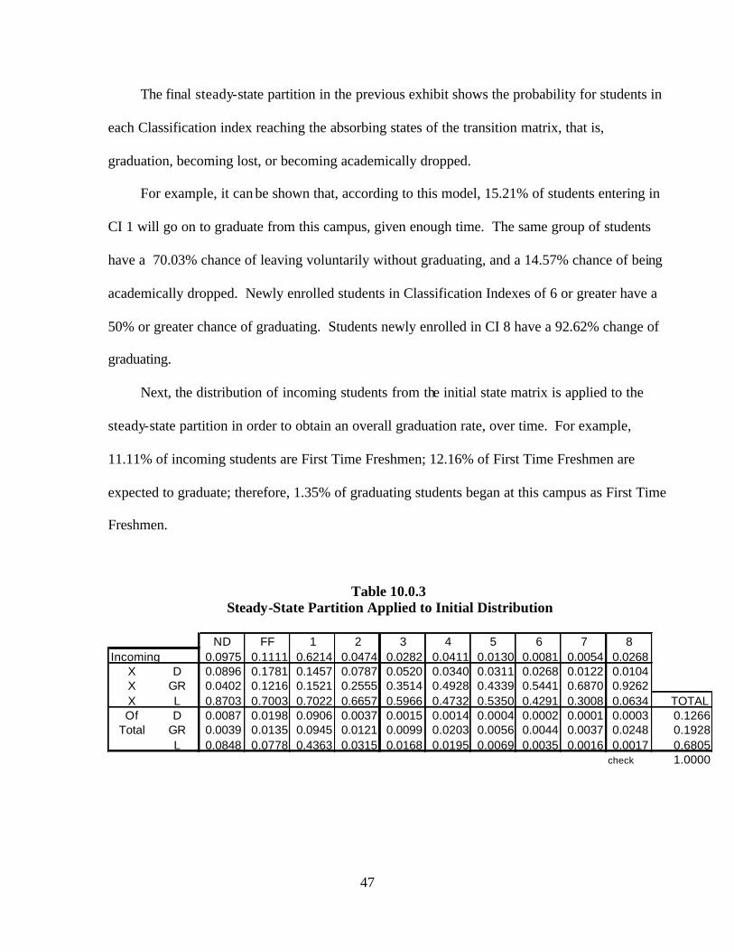
The final steady-state partition in the previous exhibit shows the probability for students in

each Classification index reaching the absorbing states of the transition matrix, that is,

graduation, becoming lost, or becoming academically dropped.

For example, it can be shown that, according to this model, 15.21% of students entering in

CI 1 will go on to graduate from this campus, given enough time. The same group of students

have a 70.03% chance of leaving voluntarily without graduating, and a 14.57% chance of being

academically dropped. Newly enrolled students in Classification Indexes of 6 or greater have a

50% or greater chance of graduating. Students newly enrolled in CI 8 have a 92.62% change of

graduating.

Next, the distribution of incoming students from the initial state matrix is applied to the

steady-state partition in order to obtain an overall graduation rate, over time. For example,

11.11% of incoming students are First Time Freshmen; 12.16% of First Time Freshmen are

expected to graduate; therefore, 1.35% of graduating students began at this campus as First Time

Freshmen.

Table 10.0.3 Steady-State Partition Applied to Initial Distribution

ND FF 1 2 3 4 5 6 7 8

Incoming 0.0975 0.1111 0.6214 0.0474 0.0282 0.0411 0.0130 0.0081 0.0054 0.0268X D 0.0896 0.1781 0.1457 0.0787 0.0520 0.0340 0.0311 0.0268 0.0122 0.0104X GR 0.0402 0.1216 0.1521 0.2555 0.3514 0.4928 0.4339 0.5441 0.6870 0.9262X L 0.8703 0.7003 0.7022 0.6657 0.5966 0.4732 0.5350 0.4291 0.3008 0.0634 TOTALOf D 0.0087 0.0198 0.0906 0.0037 0.0015 0.0014 0.0004 0.0002 0.0001 0.0003 0.1266

Total GR 0.0039 0.0135 0.0945 0.0121 0.0099 0.0203 0.0056 0.0044 0.0037 0.0248 0.1928L 0.0848 0.0778 0.4363 0.0315 0.0168 0.0195 0.0069 0.0035 0.0016 0.0017 0.6805

check 1.0000

48

Over enough time, 19.28% of the distribution of incoming students will graduate, 68.05%

will leave the university voluntarily without graduating, and 12.66% will be academically

dropped.

Variations of this same steady-state model were developed to show the eventual outcomes

of other specific groups of students, particularly students grouped by age, full- or part-time

status, and degree group. The next several sections will detail the development of these models,

and analyze the results.

10.1 The Steady-State Model Applied to Hours Enrolled and Classification Index

Using the same methods to develop the steady-state model above, data was sorted and

summarized to create a transition matrix whose states were first grouped by full-time or part-time

enrollment, and then by Classification Index within those two groupings. The partitioned steady

state matrix, by hours enrolled and Classification Index follows. The matrices required to

develop the steady-state matrix for this grouping of data will also follow.

Table 10.1.1

Partitioned Transition Matrix by Hours Registered and CI

X X X ND FF 1 2 3 4 5 6 7 8 ND FF 1 2 3 4 5 6 7 8D GR L

X D 1.0000 0.0806 0.1538 0.0705 0.0276 0.0169 0.0105 0.0031 0.0049 0.0018 0.0848 0.2847 0.1051 0.0299 0.0165 0.0100 0.0084 0.0164 0.0030 0.0013

X GR 1.0000 0.0646 0.0047 0.0016 0.0077 0.5662 0.0011 0.1594 0.0209 0.0117 0.0122 0.4116

X L 1.0000 0.2419 0.1381 0.1363 0.1472 0.1408 0.0929 0.1011 0.1024 0.1673 0.0236 0.4214 0.2918 0.2334 0.2249 0.2196 0.1253 0.2469 0.2061 0.1738 0.0264

ND 0.1452 0.0152

FF 0.0063

1 0.1774 0.4063 0.2802 0.0086 0.0045 0.0018 0.0047 0.0049 0.0038 0.0054 0.0455 0.1459 0.0943 0.0023 0.0007 0.0047 0.0061 0.0040

2 0.0323 0.1893 0.3204 0.0988 0.0056 0.0023 0.0093 0.0407 0.0019 0.0054 0.0501 0.0575 0.0023 0.0003 0.0021 0.0047 - -

3 0.0227 0.5032 0.1025 0.0092 0.0016 0.0033 0.0038 0.0018 0.0023 0.0715 0.0616 0.0010 0.0042 - 0.0030 -

4 0.0036 0.0492 0.5163 0.3407 0.0202 0.0179 0.0096 0.0073 0.0007 0.0027 0.0696 0.0675 0.0063 0.0047 0.0061 0.0040

5 0.0007 0.0039 0.0242 0.1983 0.1244 0.0065 0.0038 - - - 0.0029 0.0152 0.0649 0.0047 - -

6 0.0011 0.0035 0.0051 0.0531 0.5163 0.1073 0.0058 0.0018 0.0009 0.0005 0.0031 0.0649 0.0796 - 0.0026

7 0.0161 0.0002 0.0004 0.0006 0.0279 0.0747 0.5187 0.0788 0.0018 0.0005 0.0010 0.0021 0.0726 0.0640 0.0013

8 0.0179 0.0140 0.0780 0.5212 0.2323 0.0005 0.0021 0.0021 0.0047 0.0915 0.1240

ND 0.1613 0.0007 0.0004 0.0016 0.3500 0.0002 0.0003

FF 0.0063

1 0.1452 0.0947 0.0925 0.0030 0.0006 0.0014 0.0016 0.0643 0.2740 0.3391 0.0095 0.0034 0.0041 0.0105 0.0047 0.0030 0.0106

2 0.0178 0.0672 0.0393 0.0006 0.0005 0.0031 0.0027 0.0036 0.1617 0.3303 0.0120 0.0031 0.0126 0.0047 - 0.0026

3 0.0031 0.1036 0.0462 0.0023 - 0.0033 0.0019 0.0009 0.0063 0.2529 0.3611 0.0100 0.0042 0.0117 0.0122 0.0040

4 0.0009 0.0099 0.1295 0.1218 0.0093 0.0065 - 0.0036 0.0009 0.0041 0.0136 0.2447 0.5072 0.0335 0.0258 0.0335 0.0567

5 0.0009 0.0045 0.0398 0.0280 - - 0.0018 0.0009 0.0014 0.0009 0.0040 0.0530 0.2866 0.0117 0.0122 0.0026

6 - 0.0011 0.0078 0.0731 0.0244 0.0038 - - 0.0005 0.0023 0.0006 0.0169 0.2113 0.2974 0.0091 0.0053

7 - 0.0006 0.0032 0.0078 0.0650 0.0288 - - 0.0002 0.0005 0.0006 0.0079 0.0167 0.2201 0.3567 0.0092

8 0.0004 0.0006 0.0041 0.0016 0.0146 0.1615 0.1470 0.0009 0.0117 0.0021 0.0141 0.2134 0.3338

check 1.0000 1.0000 1.0000 1.0000 1.0000 1.0000 1.0000 1.0000 1.0000 1.0000 1.0000 1.0000 1.0000 1.0000 1.0000 1.0000 1.0000 1.0000 1.0000 1.0000 1.0000 1.0000 1.0000

CURRENT

NE

XT

Full-time Part-time

Full-

time

Par

t-tim

e

49

50

Table 10.1.2 Steady-State Calculation by Hours Registered and CI

Identity Matrix

1.0000

1.00001.0000

1.00001.0000

1.00001.0000

1.00001.0000

1.00001.0000

1.00001.0000

1.00001.0000

1.00001.0000

1.00001.0000

1.0000


0.1452 0.0152

0.0063

0.1774 0.4063 0.2802 0.0086 0.0045 0.0018 0.0047 0.0049 0.0038 0.0054 0.0455 0.1459 0.0943 0.0023 0.0007 0.0047 0.0061 0.0040

0.0323 0.1893 0.3204 0.0988 0.0056 0.0023 0.0093 0.0407 0.0019 0.0054 0.0501 0.0575 0.0023 0.0003 0.0021 0.0047 - - 0.0227 0.5032 0.1025 0.0092 0.0016 0.0033 0.0038 0.0018 0.0023 0.0715 0.0616 0.0010 0.0042 - 0.0030 -

0.0036 0.0492 0.5163 0.3407 0.0202 0.0179 0.0096 0.0073 0.0007 0.0027 0.0696 0.0675 0.0063 0.0047 0.0061 0.0040

0.0007 0.0039 0.0242 0.1983 0.1244 0.0065 0.0038 - - - 0.0029 0.0152 0.0649 0.0047 - -

0.0011 0.0035 0.0051 0.0531 0.5163 0.1073 0.0058 0.0018 0.0009 0.0005 0.0031 0.0649 0.0796 - 0.0026 0.0161 0.0002 0.0004 0.0006 0.0279 0.0747 0.5187 0.0788 0.0018 0.0005 0.0010 0.0021 0.0726 0.0640 0.0013

0.0179 0.0140 0.0780 0.5212 0.2323 0.0005 0.0021 0.0021 0.0047 0.0915 0.1240

0.1613 0.0007 0.0004 0.0016 0.3500 0.0002 0.0003

0.0063

0.1452 0.0947 0.0925 0.0030 0.0006 0.0014 0.0016 0.0643 0.2740 0.3391 0.0095 0.0034 0.0041 0.0105 0.0047 0.0030 0.0106 0.0178 0.0672 0.0393 0.0006 0.0005 0.0031 0.0027 0.0036 0.1617 0.3303 0.0120 0.0031 0.0126 0.0047 - 0.0026

0.0031 0.1036 0.0462 0.0023 - 0.0033 0.0019 0.0009 0.0063 0.2529 0.3611 0.0100 0.0042 0.0117 0.0122 0.0040

0.0009 0.0099 0.1295 0.1218 0.0093 0.0065 - 0.0036 0.0009 0.0041 0.0136 0.2447 0.5072 0.0335 0.0258 0.0335 0.0567

0.0009 0.0045 0.0398 0.0280 - - 0.0018 0.0009 0.0014 0.0009 0.0040 0.0530 0.2866 0.0117 0.0122 0.0026 - 0.0011 0.0078 0.0731 0.0244 0.0038 - - 0.0005 0.0023 0.0006 0.0169 0.2113 0.2974 0.0091 0.0053

- 0.0006 0.0032 0.0078 0.0650 0.0288 - - 0.0002 0.0005 0.0006 0.0079 0.0167 0.2201 0.3567 0.0092

0.0004 0.0006 0.0041 0.0016 0.0146 0.1615 0.1470 0.0009 0.0117 0.0021 0.0141 0.2134 0.3338

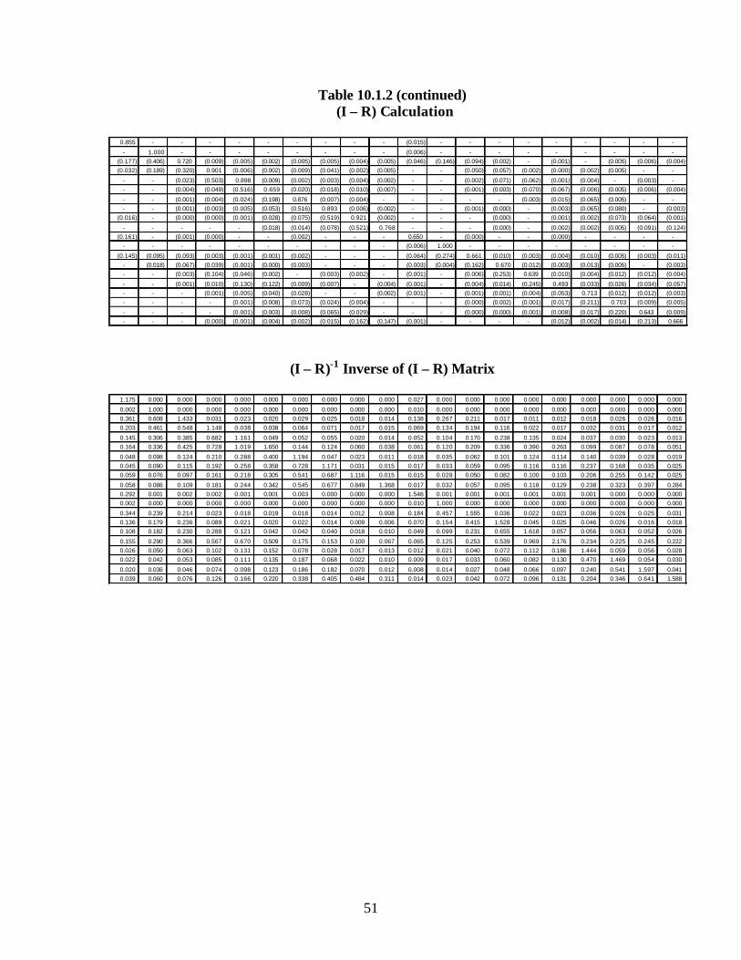
51

Table 10.1.2 (continued) (I – R) Calculation

0.855 - - - - - - - - - (0.015) - - - - - - - - -

- 1.000 - - - - - - - - (0.006) - - - - - - - - - (0.177) (0.406) 0.720 (0.009) (0.005) (0.002) (0.005) (0.005) (0.004) (0.005) (0.046) (0.146) (0.094) (0.002) - (0.001) - (0.005) (0.006) (0.004) (0.032) (0.189) (0.320) 0.901 (0.006) (0.002) (0.009) (0.041) (0.002) (0.005) - - (0.050) (0.057) (0.002) (0.000) (0.002) (0.005) - -

- - (0.023) (0.503) 0.898 (0.009) (0.002) (0.003) (0.004) (0.002) - - (0.002) (0.071) (0.062) (0.001) (0.004) - (0.003) - - - (0.004) (0.049) (0.516) 0.659 (0.020) (0.018) (0.010) (0.007) - - (0.001) (0.003) (0.070) (0.067) (0.006) (0.005) (0.006) (0.004)

- - (0.001) (0.004) (0.024) (0.198) 0.876 (0.007) (0.004) - - - - - (0.003) (0.015) (0.065) (0.005) - - - - (0.001) (0.003) (0.005) (0.053) (0.516) 0.893 (0.006) (0.002) - - (0.001) (0.000) - (0.003) (0.065) (0.080) - (0.003)

(0.016) - (0.000) (0.000) (0.001) (0.028) (0.075) (0.519) 0.921 (0.002) - - - (0.000) - (0.001) (0.002) (0.073) (0.064) (0.001)

- - - - - (0.018) (0.014) (0.078) (0.521) 0.768 - - - (0.000) - (0.002) (0.002) (0.005) (0.091) (0.124) (0.161) - (0.001) (0.000) - - (0.002) - - - 0.650 - (0.000) - - (0.000) - - - -

- - - - - - - - - - (0.006) 1.000 - - - - - - - -

(0.145) (0.095) (0.093) (0.003) (0.001) (0.001) (0.002) - - - (0.064) (0.274) 0.661 (0.010) (0.003) (0.004) (0.010) (0.005) (0.003) (0.011) - (0.018) (0.067) (0.039) (0.001) (0.000) (0.003) - - - (0.003) (0.004) (0.162) 0.670 (0.012) (0.003) (0.013) (0.005) - (0.003) - - (0.003) (0.104) (0.046) (0.002) - (0.003) (0.002) - (0.001) - (0.006) (0.253) 0.639 (0.010) (0.004) (0.012) (0.012) (0.004)

- - (0.001) (0.010) (0.130) (0.122) (0.009) (0.007) - (0.004) (0.001) - (0.004) (0.014) (0.245) 0.493 (0.033) (0.026) (0.034) (0.057) - - - (0.001) (0.005) (0.040) (0.028) - - (0.002) (0.001) - (0.001) (0.001) (0.004) (0.053) 0.713 (0.012) (0.012) (0.003) - - - - (0.001) (0.008) (0.073) (0.024) (0.004) - - - (0.000) (0.002) (0.001) (0.017) (0.211) 0.703 (0.009) (0.005)

- - - - (0.001) (0.003) (0.008) (0.065) (0.029) - - - (0.000) (0.000) (0.001) (0.008) (0.017) (0.220) 0.643 (0.009) - - - (0.000) (0.001) (0.004) (0.002) (0.015) (0.162) (0.147) (0.001) - - - - (0.012) (0.002) (0.014) (0.213) 0.666

(I – R)-1 Inverse of (I – R) Matrix

1.175 0.000 0.000 0.000 0.000 0.000 0.000 0.000 0.000 0.000 0.027 0.000 0.000 0.000 0.000 0.000 0.000 0.000 0.000 0.000

0.002 1.000 0.000 0.000 0.000 0.000 0.000 0.000 0.000 0.000 0.010 0.000 0.000 0.000 0.000 0.000 0.000 0.000 0.000 0.000 0.361 0.608 1.433 0.031 0.023 0.020 0.029 0.025 0.018 0.014 0.138 0.267 0.211 0.017 0.011 0.012 0.018 0.026 0.026 0.016 0.203 0.461 0.548 1.148 0.038 0.038 0.064 0.071 0.017 0.015 0.069 0.134 0.194 0.116 0.022 0.017 0.032 0.031 0.017 0.012

0.145 0.306 0.385 0.682 1.161 0.049 0.052 0.055 0.020 0.014 0.052 0.104 0.170 0.238 0.135 0.024 0.037 0.030 0.023 0.013 0.164 0.336 0.425 0.728 1.019 1.650 0.144 0.124 0.060 0.038 0.061 0.120 0.209 0.336 0.390 0.263 0.099 0.087 0.078 0.051

0.048 0.098 0.124 0.210 0.288 0.400 1.194 0.047 0.023 0.011 0.018 0.035 0.062 0.101 0.124 0.114 0.140 0.039 0.028 0.019 0.045 0.090 0.115 0.192 0.258 0.358 0.728 1.171 0.031 0.015 0.017 0.033 0.059 0.095 0.116 0.116 0.237 0.168 0.035 0.025 0.059 0.076 0.097 0.161 0.218 0.305 0.541 0.687 1.116 0.015 0.015 0.028 0.050 0.082 0.100 0.103 0.206 0.255 0.142 0.025

0.058 0.086 0.109 0.181 0.244 0.342 0.545 0.677 0.849 1.368 0.017 0.032 0.057 0.095 0.118 0.129 0.238 0.323 0.397 0.284 0.292 0.001 0.002 0.002 0.001 0.001 0.003 0.000 0.000 0.000 1.546 0.001 0.001 0.001 0.001 0.001 0.001 0.000 0.000 0.000 0.002 0.000 0.000 0.000 0.000 0.000 0.000 0.000 0.000 0.000 0.010 1.000 0.000 0.000 0.000 0.000 0.000 0.000 0.000 0.000

0.344 0.239 0.214 0.023 0.018 0.019 0.018 0.014 0.012 0.008 0.184 0.457 1.555 0.036 0.022 0.023 0.036 0.026 0.025 0.031 0.136 0.179 0.236 0.089 0.021 0.020 0.022 0.014 0.009 0.006 0.070 0.154 0.415 1.528 0.045 0.025 0.046 0.026 0.016 0.018 0.108 0.182 0.230 0.288 0.121 0.042 0.042 0.040 0.018 0.010 0.049 0.099 0.231 0.655 1.618 0.057 0.056 0.063 0.052 0.026

0.155 0.290 0.366 0.567 0.670 0.509 0.175 0.153 0.100 0.067 0.065 0.125 0.253 0.539 0.969 2.176 0.234 0.225 0.245 0.222 0.026 0.050 0.063 0.102 0.131 0.152 0.078 0.028 0.017 0.013 0.012 0.021 0.040 0.072 0.112 0.186 1.444 0.059 0.056 0.028 0.022 0.042 0.053 0.085 0.111 0.135 0.187 0.068 0.022 0.010 0.009 0.017 0.033 0.060 0.082 0.130 0.470 1.469 0.054 0.030

0.020 0.036 0.046 0.074 0.098 0.123 0.186 0.182 0.070 0.012 0.008 0.014 0.027 0.048 0.066 0.097 0.240 0.541 1.597 0.041 0.039 0.060 0.076 0.126 0.166 0.220 0.338 0.405 0.484 0.311 0.014 0.023 0.042 0.072 0.096 0.131 0.204 0.346 0.641 1.588

52

Table 10.1.2 (continued) S Partition of Transition Matrix

0.0806 0.1538 0.0705 0.0276 0.0169 0.0105 0.0031 0.0049 - 0.0018 0.0848 0.2847 0.1051 0.0299 0.0165 0.0100 0.0084 0.0164 0.0030 0.0013

- - - - - 0.0646 0.0047 0.0016 0.0077 0.5662 - - - - 0.0011 0.1594 0.0209 0.0117 0.0122 0.4116

0.2419 0.1381 0.1363 0.1472 0.1408 0.0929 0.1011 0.1024 0.1673 0.0236 0.4214 0.2918 0.2334 0.2249 0.2196 0.1253 0.2469 0.2061 0.1738 0.0264


0.2003 0.2569 0.1672 0.0733 0.0504 0.0369 0.0245 0.0196 0.0087 0.0072 0.1741 0.3667 0.2092 0.0804 0.0517 0.0358 0.0351 0.0391 0.018 0.01230.0865 0.1444 0.1829 0.2985 0.3883 0.4832 0.5021 0.5939 0.7102 0.9163 0.0308 0.0565 0.1062 0.1957 0.2933 0.499 0.3037 0.3945 0.5551 0.85480.7132 0.5987 0.6499 0.6282 0.5613 0.4799 0.4734 0.3866 0.2811 0.0764 0.7952 0.5768 0.6847 0.7239 0.655 0.4652 0.6612 0.5664 0.4269 0.1329


ND FF 1 2 3 4 5 6 7 8 ND FF 1 2 3 4 5 6 7 8

X D 0.2003 0.2569 0.1672 0.0733 0.0504 0.0369 0.0245 0.0196 0.0087 0.0072 0.1741 0.3667 0.2092 0.0804 0.0517 0.0358 0.0351 0.0391 0.018 0.0123X GR 0.0865 0.1444 0.1829 0.2985 0.3883 0.4832 0.5021 0.5939 0.7102 0.9163 0.0308 0.0565 0.1062 0.1957 0.2933 0.499 0.3037 0.3945 0.5551 0.8548X L 0.7132 0.5987 0.6499 0.6282 0.5613 0.4799 0.4734 0.3866 0.2811 0.0764 0.7952 0.5768 0.6847 0.7239 0.655 0.4652 0.6612 0.5664 0.4269 0.1329

check 1.0000 1.0000 1.0000 1.0000 1.0000 1.0000 1.0000 1.0000 1.0000 1.0000 1.0000 1.0000 1.0000 1.0000 1.0000 1.0000 1.0000 1.0000 1.0000 1.0000

Full-time Part-time

The distribution of incoming students grouped by hours registered and CI is applied to the

steady-state partition in order to obtain an overall graduation rate, over time.

Over time, the graduation rates for full-time and part-time students vary little. Based on

this model, full-time students can be expected to graduate at a rate of 20.01% while part-time

students have an expected graduation rate of 24.29%. Of full- time students, 62.91% can be

expected to leave the university without graduating, and 17.08% will be academically dropped.

Of part-time students, 60.83% will leave the university voluntarily without graduating, and

14.88% will be academically dropped.

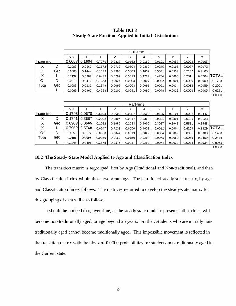
53


ND FF 1 2 3 4 5 6 7 8Incoming 0.0097 0.1604 0.7376 0.0328 0.0162 0.0187 0.0101 0.0058 0.0022 0.0065

X D 0.2003 0.2569 0.1672 0.0733 0.0504 0.0369 0.0245 0.0196 0.0087 0.0072 X GR 0.0865 0.1444 0.1829 0.2985 0.3883 0.4832 0.5021 0.5939 0.7102 0.9163 X L 0.7132 0.5987 0.6499 0.6282 0.5613 0.4799 0.4734 0.3866 0.2811 0.0764 TOTALOf D 0.0019 0.0412 0.1233 0.0024 0.0008 0.0007 0.0002 0.0001 0.0000 0.0000 0.1708

Total GR 0.0008 0.0232 0.1349 0.0098 0.0063 0.0091 0.0051 0.0034 0.0015 0.0059 0.2001 L 0.0069 0.0960 0.4793 0.0206 0.0091 0.0090 0.0048 0.0022 0.0006 0.0005 0.6291

1.0000

ND FF 1 2 3 4 5 6 7 8Incoming 0.1746 0.0678 0.5193 0.0602 0.0387 0.0608 0.0155 0.0101 0.0082 0.0447


Total GR 0.0151 0.0098 0.0950 0.0180 0.0150 0.0294 0.0078 0.0060 0.0059 0.0409 0.2429 L 0.1245 0.0406 0.3375 0.0378 0.0217 0.0292 0.0074 0.0039 0.0023 0.0034 0.6083

1.0000

Part-time

Full-time

10.2 The Steady-State Model Applied to Age and Classification Index

The transition matrix is regrouped, first by Age (Traditional and Non-traditional), and then

by Classification Index within those two groupings. The partitioned steady state matrix, by age

and Classification Index follows. The matrices required to develop the steady-state matrix for

this grouping of data will also follow.

It should be noticed that, over time, as the steady-state model represents, all students will

become non-traditionally aged, or age beyond 25 years. Further, students who are initially non-

traditionally aged cannot become traditionally aged. This impossible movement is reflected in

the transition matrix with the block of 0.0000 probabilities for students non-traditionally aged in

the Current state.

Table 10.2.1 Partitioned Trans ition Matrix by Age and CI

X X X ND FF 1 2 3 4 5 6 7 8 ND FF 1 2 3 4 5 6 7 8D GR L

X D 1.0000 0.0886 0.2073 0.1018 0.0362 0.0253 0.0170 0.0078 0.0158 0.0020 0.0777 0.1375 0.0496 0.0150 0.0042 0.0028 0.0042 0.0021 0.0025 0.0013

X GR 1.0000 - - - - - 0.1026 0.0155 0.0053 0.0110 0.5930 - - - - 0.0014 0.1309 0.0063 0.0042 0.0076 0.4356 X L 1.0000 0.3892 0.1819 0.1801 0.1827 0.1780 0.0954 0.1366 0.1090 0.1744 0.4329 0.2875 0.2171 0.1900 0.1827 0.1329 0.1987 0.1878 0.1641

ND 0.3544 0.0005 0.0003 0.0004 0.0016 FF 0.0174 - 0.0003 - -

1 0.1345 0.4683 0.3840 0.0126 0.0029 0.0034 0.0109 0.0018 0.0044 0.0039

2 0.0032 0.1368 0.2933 0.2107 0.0095 0.0030 0.0109 0.0105 - 0.0020 3 0.0016 0.0160 0.4858 0.2305 0.0121 0.0031 0.0070 0.0088 -

4 0.0039 0.0393 0.5079 0.4818 0.0233 0.0246 0.0155 0.0117

5 0.0006 0.0020 0.0177 0.1730 0.1894 0.0123 0.0066 0.0020 6 0.0011 0.0020 0.0043 0.0397 0.5000 0.1687 0.0110 0.0059

7 0.0002 0.0007 0.0208 0.0512 0.5255 0.1435 0.0020

8 0.0002 0.0003 0.0144 0.0140 0.0826 0.5894 0.3405 ND 0.0079 0.3675 0.0008 0.0004

FF - 0.0053 - -

1 0.0032 0.0056 0.0113 0.0005 0.1025 0.4625 0.4106 0.0100 0.0063 0.0049 0.0042 0.0127 0.0076 0.0152 2 0.0064 0.0079 - 0.0071 0.1125 0.2935 0.3364 0.0112 0.0032 0.0167 0.0084 0.0025 0.0051

3 0.0006 0.0167 0.0100 0.0008 0.0022 0.0018 0.0182 0.4056 0.3487 0.0089 0.0063 0.0127 0.0076 0.0051

4 - 0.0017 0.0129 0.0280 0.0031 0.0053 - 0.0039 0.0018 0.0066 0.0336 0.4233 0.5466 0.0439 0.0232 0.0278 0.0568 5 - 0.0003 0.0005 0.0053 0.0109 0.0018 - - 0.0018 0.0019 0.0037 0.0174 0.1005 0.2866 0.0105 0.0076 0.0025

6 0.0002 0.0003 0.0004 0.0140 0.0105 - - 0.0018 0.0012 0.0044 0.0021 0.0344 0.3766 0.3017 0.0076 0.0051

7 0.0011 0.0078 0.0176 0.0088 - 0.0004 0.0006 0.0021 0.0150 0.0502 0.4008 0.3157 0.0101 8 0.0008 0.0018 0.0243 0.0333 0.0006 0.0007 0.0194 0.0063 0.0359 0.4495 0.4634

check 1.0000 1.0000 1.0000 1.0000 1.0000 1.0000 1.0000 1.0000 1.0000 1.0000 1.0000 1.0000 1.0000 1.0000 1.0000 1.0000 1.0000 1.0000 1.0000 1.0000 1.0000 1.0000 1.0000

CURRENTTraditional Non-Traditional

Tra

ditio

nal

Non

-Tra

ditio

nal

54

55

Table 10.2.2 Steady-State Calculation by State and CI

Identity Matrix

1.0000

1.00001.0000

1.00001.0000

1.00001.0000

1.00001.0000

1.00001.0000

1.00001.0000

1.00001.0000

1.00001.0000

1.00001.0000

1.0000


0.3544 0.0005 0.0003 0.0004 0.0016

0.0174 - 0.0003 - -

0.1345 0.4683 0.3840 0.0126 0.0029 0.0034 0.0109 0.0018 0.0044 0.0039 0.0032 0.1368 0.2933 0.2107 0.0095 0.0030 0.0109 0.0105 - 0.0020

0.0016 0.0160 0.4858 0.2305 0.0121 0.0031 0.0070 0.0088 - 0.0039 0.0393 0.5079 0.4818 0.0233 0.0246 0.0155 0.0117

0.0006 0.0020 0.0177 0.1730 0.1894 0.0123 0.0066 0.0020 0.0011 0.0020 0.0043 0.0397 0.5000 0.1687 0.0110 0.0059

0.0002 0.0007 0.0208 0.0512 0.5255 0.1435 0.0020 0.0002 0.0003 0.0144 0.0140 0.0826 0.5894 0.3405

0.0079 0.3675 0.0008 0.0004

- 0.0053 - - 0.0032 0.0056 0.0113 0.0005 0.1025 0.4625 0.4106 0.0100 0.0063 0.0049 0.0042 0.0127 0.0076 0.0152

0.0064 0.0079 - 0.0071 0.1125 0.2935 0.3364 0.0112 0.0032 0.0167 0.0084 0.0025 0.0051 0.0006 0.0167 0.0100 0.0008 0.0022 0.0018 0.0182 0.4056 0.3487 0.0089 0.0063 0.0127 0.0076 0.0051

- 0.0017 0.0129 0.0280 0.0031 0.0053 - 0.0039 0.0018 0.0066 0.0336 0.4233 0.5466 0.0439 0.0232 0.0278 0.0568 - 0.0003 0.0005 0.0053 0.0109 0.0018 - - 0.0018 0.0019 0.0037 0.0174 0.1005 0.2866 0.0105 0.0076 0.0025

0.0002 0.0003 0.0004 0.0140 0.0105 - - 0.0018 0.0012 0.0044 0.0021 0.0344 0.3766 0.3017 0.0076 0.0051 0.0011 0.0078 0.0176 0.0088 - 0.0004 0.0006 0.0021 0.0150 0.0502 0.4008 0.3157 0.0101

0.0008 0.0018 0.0243 0.0333 0.0006 0.0007 0.0194 0.0063 0.0359 0.4495 0.4634

56

Table 10.2.2 (continued) (I – R) Calculation

0.646 - (0.000) (0.000) - (0.000) (0.002) - - - - - - - - - - - - -

(0.017) 1.000 - (0.000) - - - - - - - - - - - - - - - -

(0.134) (0.468) 0.616 (0.013) (0.003) (0.003) (0.011) (0.002) (0.004) (0.004) - - - - - - - - - -

(0.003) (0.137) (0.293) 0.789 (0.010) (0.003) (0.011) (0.011) - (0.002) - - - - - - - - - -

(0.002) - (0.016) (0.486) 0.769 (0.012) (0.003) (0.007) (0.009) - - - - - - - - - - -

- - (0.004) (0.039) (0.508) 0.518 (0.023) (0.025) (0.015) (0.012) - - - - - - - - - -

- - (0.001) (0.002) (0.018) (0.173) 0.811 (0.012) (0.007) (0.002) - - - - - - - - - -

- - (0.001) (0.002) (0.004) (0.040) (0.500) 0.831 (0.011) (0.006) - - - - - - - - - -

- - (0.000) (0.001) - (0.021) (0.051) (0.525) 0.857 (0.002) - - - - - - - - - -

- - (0.000) (0.000) - (0.014) (0.014) (0.083) (0.589) 0.659 - - - - - - - - - -

(0.008) - - - - - - - - - 0.633 - (0.001) - - (0.000) - - - -

- - - - - - - - - - (0.005) 1.000 - - - - - - - -

(0.003) (0.006) (0.011) - (0.000) - - - - - (0.102) (0.463) 0.589 (0.010) (0.006) (0.005) (0.004) (0.013) (0.008) (0.015)

- - (0.006) (0.008) - - - - - - (0.007) (0.113) (0.294) 0.664 (0.011) (0.003) (0.017) (0.008) (0.003) (0.005)

- - (0.001) (0.017) (0.010) (0.001) - - (0.002) - (0.002) - (0.018) (0.406) 0.651 (0.009) (0.006) (0.013) (0.008) (0.005)

- - - (0.002) (0.013) (0.028) (0.003) (0.005) - (0.004) (0.002) - (0.007) (0.034) (0.423) 0.453 (0.044) (0.023) (0.028) (0.057)

- - - (0.000) (0.000) (0.005) (0.011) (0.002) - - (0.002) - (0.002) (0.004) (0.017) (0.100) 0.713 (0.011) (0.008) (0.003)

- - (0.000) (0.000) - (0.000) (0.014) (0.011) - - (0.002) - (0.001) (0.004) (0.002) (0.034) (0.377) 0.698 (0.008) (0.005)

- - - - - (0.001) (0.008) (0.018) (0.009) - - - (0.000) (0.001) (0.002) (0.015) (0.050) (0.401) 0.684 (0.010)

- - - - - (0.001) - (0.002) (0.024) (0.033) - - - (0.001) (0.001) (0.019) (0.006) (0.036) (0.449) 0.537


1.550 0.001 0.002 0.002 0.002 0.002 0.003 0.000 0.000 0.000 - - - - - - - - - -

0.027 1.000 0.000 0.000 0.000 0.000 0.000 0.000 0.000 0.000 - - - - - - - - - -

0.364 0.776 1.645 0.044 0.025 0.026 0.036 0.017 0.017 0.011 - - - - - - - - - -

0.149 0.470 0.622 1.303 0.040 0.030 0.045 0.027 0.011 0.009 - - - - - - - - - -

0.107 0.320 0.437 0.843 1.353 0.061 0.051 0.041 0.023 0.007 - - - - - - - - - -

0.123 0.366 0.504 0.954 1.370 2.047 0.181 0.148 0.088 0.044 - - - - - - - - - -

0.030 0.089 0.122 0.230 0.329 0.447 1.292 0.060 0.032 0.014 - - - - - - - - - - 0.026 0.076 0.105 0.195 0.275 0.374 0.798 1.263 0.047 0.022 - - - - - - - - - -

0.021 0.062 0.085 0.158 0.222 0.307 0.573 0.784 1.203 0.019 - - - - - - - - - -

0.025 0.075 0.104 0.192 0.270 0.375 0.643 0.863 1.084 1.537 - - - - - - - - - -

0.019 0.000 0.000 0.000 0.000 0.000 0.000 0.000 0.000 0.000 1.581 0.001 0.003 0.001 0.001 0.002 0.000 0.000 0.000 0.000

0.000 0.000 0.000 0.000 0.000 0.000 0.000 0.000 0.000 0.000 0.008 1.000 0.000 0.000 0.000 0.000 0.000 0.000 0.000 0.000

0.020 0.028 0.036 0.008 0.008 0.007 0.008 0.007 0.005 0.004 0.288 0.806 1.728 0.058 0.048 0.043 0.058 0.073 0.060 0.056

0.015 0.027 0.042 0.023 0.008 0.008 0.008 0.007 0.005 0.003 0.149 0.538 0.782 1.564 0.068 0.048 0.084 0.067 0.048 0.044 0.017 0.038 0.055 0.067 0.035 0.016 0.015 0.012 0.010 0.004 0.108 0.366 0.549 0.999 1.612 0.079 0.102 0.096 0.067 0.051

0.032 0.081 0.114 0.175 0.184 0.179 0.082 0.072 0.048 0.035 0.131 0.417 0.631 1.109 1.592 2.391 0.401 0.348 0.336 0.308

0.007 0.018 0.025 0.040 0.045 0.050 0.037 0.018 0.009 0.006 0.027 0.074 0.114 0.194 0.271 0.348 1.482 0.087 0.072 0.054

0.007 0.018 0.025 0.040 0.046 0.053 0.064 0.035 0.010 0.007 0.027 0.068 0.104 0.175 0.234 0.311 0.831 1.513 0.082 0.059

0.007 0.018 0.026 0.043 0.052 0.063 0.087 0.069 0.027 0.008 0.022 0.057 0.088 0.148 0.200 0.266 0.614 0.914 1.542 0.074

0.010 0.028 0.039 0.067 0.083 0.104 0.150 0.157 0.147 0.104 0.026 0.070 0.106 0.181 0.246 0.334 0.602 0.880 1.310 1.942

57


0.0886 0.2073 0.1018 0.0362 0.0253 0.0170 0.0078 0.0158 - 0.0020 0.0777 0.1375 0.0496 0.0150 0.0042 0.0028 0.0042 0.0021 0.0025 0.0013

- - - - - 0.1026 0.0155 0.0053 0.0110 0.5930 - - - - 0.0014 0.1309 0.0063 0.0042 0.0076 0.4356

0.3892 0.1819 0.1801 0.1827 0.1780 0.0954 0.1366 0.1090 0.1744 - 0.4329 0.2875 0.2171 0.1900 0.1827 0.1329 0.1987 0.1878 0.1641 -


0.1938 0.3222 0.2159 0.0967 0.0708 0.0522 0.0355 0.0297 0.0082 0.0063 0.1417 0.189 0.1028 0.0354 0.0172 0.0133 0.016 0.013 0.011 0.00760.0372 0.1077 0.1492 0.2709 0.3711 0.5148 0.5078 0.622 0.7364 0.9667 0.0289 0.0865 0.1315 0.2287 0.3222 0.4641 0.3322 0.4431 0.6272 0.8873

0.769 0.5701 0.6349 0.6324 0.558 0.433 0.4567 0.3484 0.2554 0.027 0.8294 0.7244 0.7657 0.7359 0.6606 0.5226 0.6519 0.5439 0.3618 0.1051


ND FF 1 2 3 4 5 6 7 8 ND FF 1 2 3 4 5 6 7 8

X D 0.1938 0.3222 0.2159 0.0967 0.0708 0.0522 0.0355 0.0297 0.0082 0.0063 0.1417 0.189 0.1028 0.0354 0.0172 0.0133 0.016 0.013 0.011 0.0076X GR 0.0372 0.1077 0.1492 0.2709 0.3711 0.5148 0.5078 0.622 0.7364 0.9667 0.0289 0.0865 0.1315 0.2287 0.3222 0.4641 0.3322 0.4431 0.6272 0.8873X L 0.769 0.5701 0.6349 0.6324 0.558 0.433 0.4567 0.3484 0.2554 0.027 0.8294 0.7244 0.7657 0.7359 0.6606 0.5226 0.6519 0.5439 0.3618 0.1051

check 1.0000 1.0000 1.0000 1.0000 1.0000 1.0000 1.0000 1.0000 1.0000 1.0000 1.0000 1.0000 1.0000 1.0000 1.0000 1.0000 1.0000 1.0000 1.0000 1.0000

Traditional Non-Traditional

The distribution of incoming students grouped by age and CI is applied to the steady-state

partition in order to obtain an overall graduation rate, over time.

Over time, the graduation rates for traditionally and non-traditionally aged students vary in

favor of the non-traditionally aged students. Based on this model, traditionally aged students can

be expected to graduate at a rate of 16.37% while non-traditionally aged students have an

expected graduation rate of 25.63%. Of traditionally aged students, 62.11% can be expected to

leave the university without graduating, and 21.52% will be academically dropped. Of non-

traditionally aged students, 57.89% will leave the university voluntarily without graduating, and

16.48% will be academically dropped.

58


ND FF 1 2 3 4 5 6 7 8Incoming 0.0813 0.1498 0.6719 0.0325 0.0176 0.0204 0.0098 0.0053 0.0033 0.0081


Total GR 0.0030 0.0161 0.1002 0.0088 0.0065 0.0105 0.0050 0.0033 0.0024 0.0078 0.1637 L 0.0625 0.0854 0.4266 0.0205 0.0098 0.0088 0.0045 0.0018 0.0008 0.0002 0.6211

1.0000

ND FF 1 2 3 4 5 6 7 8Incoming 0.1302 0.0327 0.5191 0.0776 0.0495 0.0832 0.0194 0.0138 0.0097 0.0648

X 0.1417 0.1890 0.1028 0.0354 0.0172 0.0133 0.0160 0.0130 0.0110 0.0076 X 0.0289 0.0865 0.1315 0.2287 0.3222 0.4641 0.3322 0.4431 0.6272 0.8873 X 0.8294 0.7244 0.7657 0.7359 0.6606 0.5226 0.6519 0.5439 0.3618 0.1051 TOTALOf D 0.0252 0.0105 0.1121 0.0075 0.0035 0.0043 0.0007 0.0004 0.0001 0.0004 0.1648

Total GR 0.0048 0.0035 0.0774 0.0210 0.0184 0.0428 0.0099 0.0086 0.0071 0.0627 0.2563 L 0.1001 0.0186 0.3296 0.0491 0.0276 0.0360 0.0089 0.0048 0.0025 0.0017 0.5789

1.0000

Non-Traditional

Traditional

10.3 The Steady-State Model Applied to Degree Groupings

The transition matrix is reclassified by Degree Groupings alone. Initially, this transition

matrix also included states by Classification Index. However, with 10 Classification Indexes, 7

Degree Groupings, and 3 reasons for becoming non-enrolled, this 73-by-73 matrix was too

unwieldy, exceeding dimension limitations for some of Excel’s matrix functions. After several

alternative attempts to compress classification indexes into fewer states, it was determined that

the transition matrix most representative of movement between data points would include only

Degree Groups, and eliminate Classification Indexes entirely.

The partitioned steady state matrix, by age and Classification Index follows. The matrices

required to develop the steady-state matrix for this grouping of data will also follow.

Table 10.3.1

Partitioned Transition Matrix by Degree Grouping

D G L AS BS BR HS PRE TR UN

D 1.0000 0.0065 0.0102 0.1470 0.0194 0.0720 0.0373 0.0847 G 1.0000 0.1253 0.0679 - - 0.0007 0.0022 0.0280 L 1.0000 0.0782 0.1395 0.1994 0.3935 0.1839 0.2729 0.3459 AS 0.4123 0.0831 0.0719 0.0290 0.1316 0.0778 0.0546 BS 0.1919 0.5703 0.0678 0.0581 0.1318 0.1857 0.0805 BR 0.0165 0.0127 0.3111 0.0335 0.0270 0.0091 HS 0.4484 PRE 0.1247 0.0715 0.1608 0.0129 0.3985 0.1106 0.0833 TR 0.0336 0.0383 0.0292 0.0258 0.0341 0.2761 0.0252 UN 0.0110 0.0066 0.0126 0.0129 0.0139 0.0103 0.2885

CURRENTN

EX

T

59

60

Table 10.3.2 Steady-State Calculation by Degree Grouping

Identity Matrix

1.0000

1.0000 1.0000

1.0000 1.0000

1.0000 1.0000


0.4123 0.0831 0.0719 0.0290 0.1316 0.0778 0.0546 0.1919 0.5703 0.0678 0.0581 0.1318 0.1857 0.0805 0.0165 0.0127 0.3111 0.0335 0.0270 0.0091

0.4484 0.1247 0.0715 0.1608 0.0129 0.3985 0.1106 0.0833 0.0336 0.0383 0.0292 0.0258 0.0341 0.2761 0.0252 0.0110 0.0066 0.0126 0.0129 0.0139 0.0103 0.2885

(I – R) Calculation

0.5877 (0.0831) (0.0719) (0.0290) (0.1316) (0.0778) (0.0546) (0.1919) 0.4297 (0.0678) (0.0581) (0.1318) (0.1857) (0.0805) (0.0165) (0.0127) 0.6889 - (0.0335) (0.0270) (0.0091)

- - - 0.5516 - - - (0.1247) (0.0715) (0.1608) (0.0129) 0.6015 (0.1106) (0.0833) (0.0336) (0.0383) (0.0292) (0.0258) (0.0341) 0.7239 (0.0252) (0.0110) (0.0066) (0.0126) (0.0129) (0.0139) (0.0103) 0.7115


2.0682 0.5673 0.4469 0.2137 0.6366 0.4863 0.3205 1.2386 2.8583 0.7019 0.4527 1.0098 1.0551 0.5833 0.1126 0.1008 1.5118 0.0266 0.1389 0.1164 0.0598 - - - 1.8129 - - -

0.6512 0.5296 0.6155 0.1706 1.9945 0.5388 0.3705 0.1988 0.2082 0.1498 0.1092 0.1847 1.4916 0.1152 0.0611 0.0504 0.0544 0.0458 0.0634 0.0516 1.4258

61


0.0065 0.0102 0.1470 0.0194 0.0720 0.0373 0.0847 0.1253 0.0679 - - 0.0007 0.0022 0.0280 0.0782 0.1395 0.1994 0.3935 0.1839 0.2729 0.3459


0.1020 0.0977 0.2868 0.0652 0.1906 0.1298 0.1686 0.3459 0.2674 0.1060 0.0592 0.1520 0.1378 0.1202 0.5521 0.6349 0.6072 0.8756 0.6574 0.7324 0.7112


AS BS BR HS PRE TR UN

D 0.1020 0.0977 0.2868 0.0652 0.1906 0.1298 0.1686 G 0.3459 0.2674 0.1060 0.0592 0.1520 0.1378 0.1202 L 0.5521 0.6349 0.6072 0.8756 0.6574 0.7324 0.7112 check 1.0000 1.0000 1.0000 1.0000 1.0000 1.0000 1.0000

The distribution of incoming students classified by Degree Groups is applied to the

steady-state partition in order to obtain an overall graduation rate, over time.


AS BS BR HS PRE TR UNIncoming 0.0732 0.1579 0.1542 0.0265 0.3839 0.0922 0.1120

X D 0.1020 0.0977 0.2868 0.0652 0.1906 0.1298 0.1686 X GR 0.3459 0.2674 0.1060 0.0592 0.1520 0.1378 0.1202 X L 0.5521 0.6349 0.6072 0.8756 0.6574 0.7324 0.7112 TOTALOf D 0.0075 0.0154 0.0442 0.0017 0.0732 0.0120 0.0189 0.173

Total GR 0.0253 0.0422 0.0163 0.0016 0.0583 0.0127 0.0135 0.170 L 0.0404 0.1003 0.0936 0.0232 0.2524 0.0675 0.0796 0.657

check 1.000

The steady-state partition applied to the initial distribution by degree group shows a

long-term graduation rate of 17%, which is similar to overall graduation rates in previous

versions of the model. By analyzing the individual groupings of the partition, it can be

62

shown that 34.59% of students seeking Associate degrees, and 26.74% of students seeking

Bachelor degrees can be expected to graduate, given enough time. Less established degree

groups such as Bridge and Undeclared have graduation rates of 10.60% and 12.02%. Of note

is the Pre group with the largest percentage of incoming students, and a long-term graduation

rate of 15.20%. Finally, of the students first admitted to this university as High School

students, 5.92% can be expected to graduate from this same campus.

10.4 Steady-State by Degree Group without Bridge Students

One potential future impact on student demographics is the reduction or elimination of

the Bridge program. Students who are found to have academic deficiencies will be required

to participate in a community college program at a different university until those

deficiencies are met.

Therefore, the last variation of the steady-state model will eliminate Bridge students

from the incoming array that is applied to the Final Steady-State Partition. Elimination of

incoming Bridge students will be the only change made to the model. The model does allow

for students to move from any other degree group to the Bridge program, should this be

necessary. This movement will still be allowed in the model. However, the new model will

not allow students who are initially classified as Bridge students to be admitted.

63

Table 10.4.1 Steady-State Partition Applied to Initial Distribution without Bridge Students

AS BS BR HS PRE TR UNIncoming 0.0866 0.1867 - 0.0313 0.4539 0.1090 0.1324

X D 0.1020 0.0977 0.2868 0.0652 0.1906 0.1298 0.1686 X GR 0.3459 0.2674 0.1060 0.0592 0.1520 0.1378 0.1202 X L 0.5521 0.6349 0.6072 0.8756 0.6574 0.7324 0.7112 TOTALOf D 0.0088 0.0182 - 0.0020 0.0865 0.0142 0.0223 0.152

Total GR 0.0300 0.0499 - 0.0019 0.0690 0.0150 0.0159 0.182 L 0.0478 0.1185 - 0.0274 0.2984 0.0799 0.0942 0.666

check 1.000

In the previous model, the Bridge students comprised approximately 15% of incoming

students. Bridge students are also shown to have an expected graduation rate of 11%.

However, the elimination of these less established students still only causes the overall

graduation rate to rise to 18.2% from 17%.

11. Summary and Analysis of Results

In this project, retention and graduation rates for several under analyzed student

classifications have been developed for the purpose aiding university retention committees in

developing guidelines for increasing retention.

11.1 First-Year Retention

It has been shown that incoming freshmen, even those with previous college

experience, are indeed more at risk for dropping out before the next academic year than

higher classification levels of students. It has also been shown that even newly enrolled

students with higher classification indexes have a significantly higher first-year retention rate

64

than newly enrolled freshmen. This suggests that higher retention rates are associated with

student capability and experience rather than continuity at a single campus.

Further, first-year retention rates also indicate that while students in good academic

standing are retained at a significantly higher rate than students on academic probation,

students in good standing are still retained at a rate of only 46%. This suggests reasons

beyond academic performance for dropping out.

Traditionally aged students have a lower first-year retention rate of 41% compared to

non-traditionally aged students at 49%. This lends some credence to the often heard notion

that more mature students perform better academically.

Full- time students are retained at a rate of 49% compared to 39% for part-time students.

This supports the statements in the literature, although it does not support the objective of

attracting more part-time students to become full- time students.

Finally, students who are admitted directly into their degree programs have much

higher retention rates at 72% for Associate degree students, and 61% for Bachelor degree

students, than students admitted into Pre or Bridge programs at 38% and 13%. Certainly

students admitted directly into their majors are more capable students than Pre or Bridge

students, but discouragement is also a factor for students who have semesters of deficiencies

to remedy before they can begin their two- or four-year programs.

11.2 Graduation Rates

Both six-year and long-term graduation rates for all students range from 17% to 25%.

Patterns in graduation rates for various student classifications are unsurprisingly similar to

first-year retention rates. Juniors and Seniors are more likely to progress to graduation than

65

Freshmen, even when the Juniors and Seniors are newly enrolled students. Non-traditionally

aged students graduate at a somewhat higher rate within the range than traditionally aged

students, but surprisingly, a higher percentage of part-time students graduate than full- time.

Finally, the highest graduation rates of 35% and 27% are seen for students in Associate

and Bachelor degree programs rather than less established programs.

12. For Further Consideration

Retention and graduation rates for specific student groups show who is being retained

and graduated, but not why this is occurring. Further research into the issue of retention will

need to take a more qualitative approach.

“Calling programs,” in which representatives of the university contact students for exit

interviews upon graduation, and to encourage enrollment by students at risk of dropping out

are commonly used at this campus. A suggestion for further study would be to institute a

randomized calling program to survey a sample of all students in order to obtain information

about needs in the areas of motivation and support.

Finally, retention rates for students using existing campus student support programs can

be developed using the methods described in this project.

66

13. References R. L. Armacost and S. Archer (2005): Spreadsheet models for program enrollment

planning. Paper presented at 2005 SAIR Conference.

R. L. Armacost and A. L. Wilson (2002): Three analytical approaches for predicting

enrollment at a growing metropolitan research university. Paper presented at the Annual

Meeting of the Association for Institutional Research (42nd, Toronto, Ontario, Canada, June

2-5, 2002.)

R. L. Armacost and A. L. Wilson (2004): Using Markov chain models to project

university and program level enrollment. Paper presented at the 2004 SAIR Annual

Conference.

R. L. Armacost, S. Archer, J. Pet-Armacost and J. Grey (2006): Using Markov chains to

assess enrollment policies. Paper presented at the 2006 AIR Annual Forum.

J. B. Dworkin (2005): Retention: How Important Is It Really? Retention and Graduation

Rates:

http://www.pnc.edu/co/Retention.pdf

Grinstead, Charles M. and J. Laurie Snell (1997): Introduction to Probability. Providence

(RI): American Mathematical Society.

67

C. R. Kraft and J. P. Jarvis (2005): An Adaptive Model for Predicting Course Enrollment

http://www.math.clemson.edu/reports/TR2005_11_KJ.pdf

Lawler, Gregory F., (1995): Introduction to Stochastic Processes. Norwell (MA): Chapman

& Hall.

Microsoft Office Online (2003): MMULT:

http://office.microsoft.com/en-us/assistance/HP052091811033.aspx

Purdue University North Central (2006): Academic Probation Information:

http://www.pnc.edu/sa/probation.html

Ross, Sheldon M., (1995): Stochastic Processes. New Jersey: Wiley.

University of Central Florida, University Analysis and Planning Support (2005): Overview of

Enrollment and Degree Projections (August 12, 2005):

http://uaps.ucf.edu/enrollment/overview.html

an enrollment retention study using a … · an enrollment retention study using a ... introduction...

Documents