an energy harvesting device for powering … · an energy harvesting device for powering rotor load...
TRANSCRIPT

The Pennsylvania State University
The Graduate School
Department of Mechanical Engineering
AN ENERGY HARVESTING DEVICE FOR POWERING ROTOR
LOAD MONITORING SENSORS
A Thesis in
Mechanical Engineering
by
David Santarelli
2010 David Santarelli
Submitted in Partial Fulfillment
of the Requirements
for the Degree of
Master of Science
May 2010

The thesis of David Santarelli was reviewed and approved* by the following:
Christopher D. Rahn
Professor of Mechanical Engineering
Thesis Co-Advisor
Edward C. Smith
Professor of Aerospace Engineering
Thesis Co-Advisor
Stephen C. Conlon
Assistant Professor of Aerospace Engineering
Thesis Co-Advisor
H. Joseph Sommer III
Professor of Mechanical Engineering
Professor-In-Charge of MNE Graduate Programs
Karen A. Thole
Professor of Mechanical Engineering
Head of the Department of Mechanical Engineering
*Signatures are on file in the Graduate School

iii
ABSTRACT
Health and Usage Monitoring Systems (HUMS) on helicopters help to determine when
dynamic, flight critical components are replaced. These systems work on the principle of
condition based maintenance and attempt to determine the usage of each component through
regime recognition. The next step to improving HUMS is to directly monitor the components
with on-board sensors that wirelessly communicate with the HUMS. This method would improve
accuracy over regime recognition and help reduce maintenance costs and increase safety. Low
power electronics, along with the desire to avoid battery replacement, make an energy harvesting
solution an attractive option to power any wireless network sensor.
This thesis presents the design of an electromagnetic energy harvester based on Faraday’s
Law of Magnetic Induction. The design space for the harvester is the hollow rod end of a pitch
link on a UH-60 Blackhawk helicopter. All of the relevant design equations relating to
electromagnetic energy harvesting are presented and each variable is looked at individually.
Three designs for an electromagnetic energy harvester that utilize the rigid motion of the pitch
link are analyzed. For each design, an analytical model was made to determine the feasibility of
implementing the design. One prototype was fabricated and tested to determine system
parameters such as mass, stiffness, damping, and performance parameters such as voltage
generated and power delivered to a load.
There is relevant circuit design presented that would be necessary to implement in the
final system. The final device is a pendulum system that uses a torsion spring and centrifugal
force to realize an effective spring and tune the device to generate power. This design was shown
to produce a maximum of 2 mW of power to a resistive load of 1000 ohms at 19 Hz excitation
and a base acceleration level of 20 m/s2.

iv
TABLE OF CONTENTS
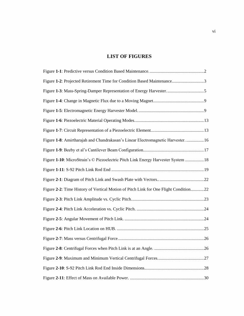
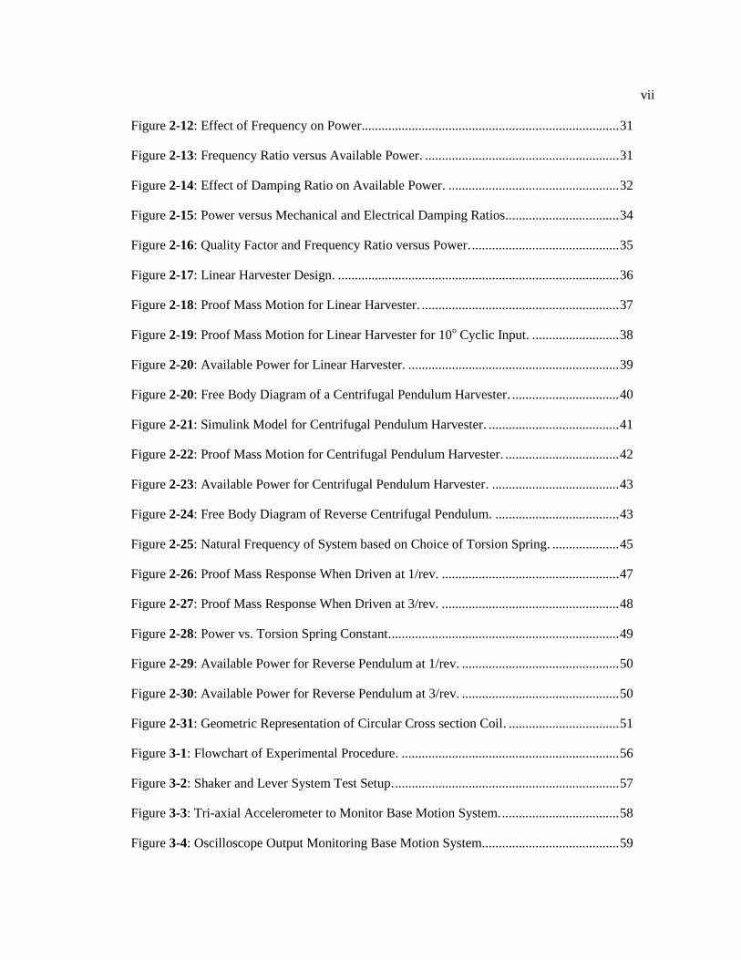
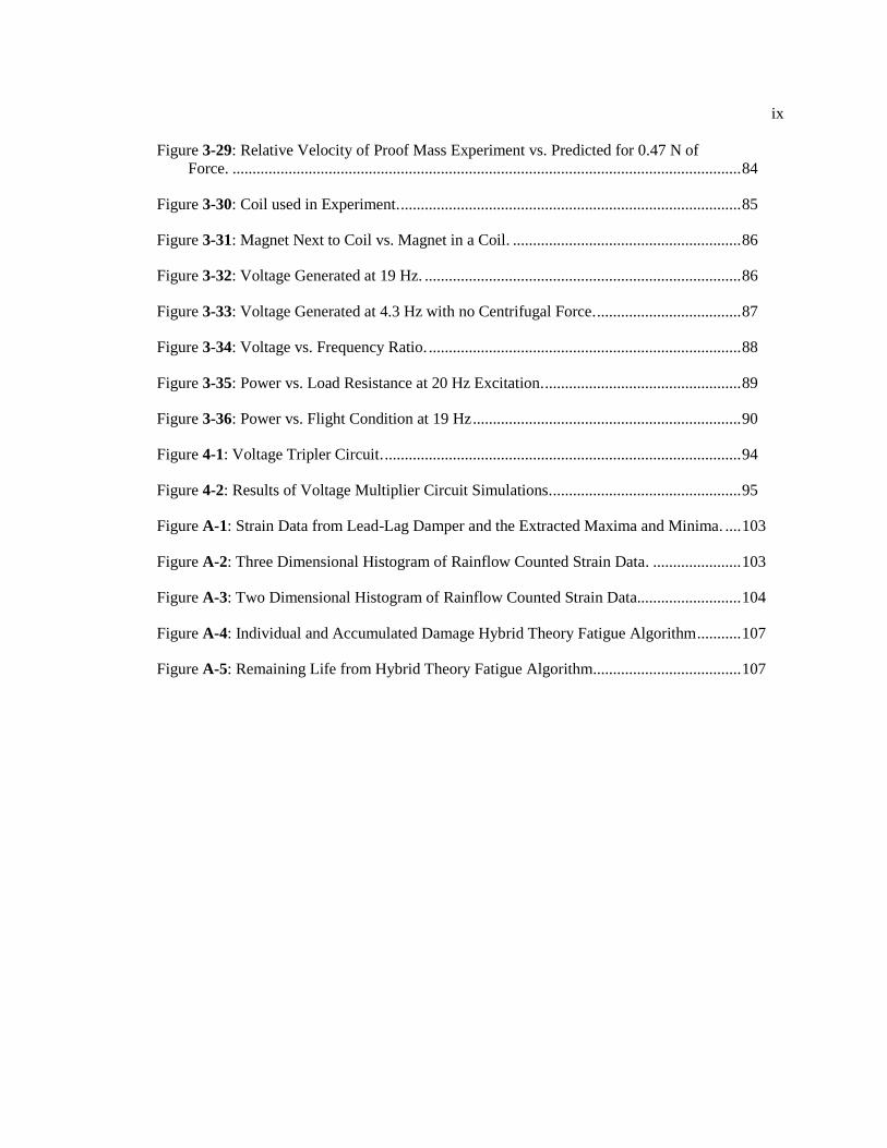
LIST OF FIGURES ................................................................................................................. vi
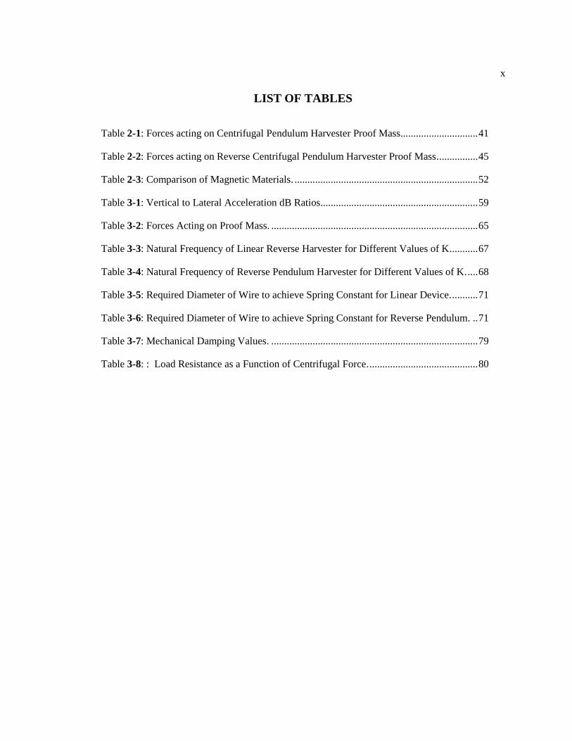
LIST OF TABLES ................................................................................................................... x
NOMENCLATURE ................................................................................................................ xi
ACKNOWLEDGEMENTS ..................................................................................................... xii
Chapter 1 Introduction ............................................................................................................ 1
1.1 Background and Motivation ....................................................................................... 1 1.2 Vibration Based Energy Harvesting ........................................................................... 4 1.2.1 Electromagnetic Implementation ......................................................................... 8 1.2.2 Piezoelectric Implementation ............................................................................... 12 1.2.3 Electrostatic Implementation ............................................................................... 14 1.3 Review of Existing Devices ....................................................................................... 15 1.4 Objectives and Goals ................................................................................................. 18
Chapter 2 Design of a New Energy Harvesting Device .......................................................... 21
2.1 Pitch Link Rod End Dynamic Environment .............................................................. 21 2.1.1 Influence of Centrifugal Forces ........................................................................... 25 2.1.2 Geometric Constraints .......................................................................................... 28 2.2 Available Power ......................................................................................................... 28 2.2.1 Effect of Mass on Available Power...................................................................... 29 2.2.2 Effect of Frequency on Available Power ............................................................. 30 2.2.3 Effect of Damping on Available Power ............................................................... 32 2.2.4 Effect of Quality Factor on Available Power ....................................................... 34 2.3 Linear Harvester Design ............................................................................................ 35 2.4 Centrifugal Pendulum Harvester Design ................................................................... 39 2.5 Reverse Centrifugal Pendulum Harvester Design ...................................................... 44 2.6 Magnet and Coil Design............................................................................................. 51
Chapter 3 Experimental Testing of Energy Harvesting Device .............................................. 55
3.1 Experimental Procedure ............................................................................................. 55 3.2 Experimental Setup .................................................................................................... 57 3.3 Fabrication of Harvester Device ................................................................................ 61 3.3.1 Torsion Spring ...................................................................................................... 67 3.4 Device Circuitry ......................................................................................................... 71 3.5 Testing of Device ....................................................................................................... 74 3.5.1 Natural Frequency Prediction and Validation ...................................................... 74 3.5.2 Mechanical and Electrical Damping .................................................................... 78 3.5.3 Mass Motion Prediction and Validation .............................................................. 81 3.5.4 Voltage Prediction and Validation ....................................................................... 84 3.6 Energy Harvesting Performance ................................................................................ 88

v
Chapter 4 Conclusion .............................................................................................................. 92
4.1 Conclusions on Energy Harvester .............................................................................. 92 4.2 Future Work ............................................................................................................... 96
References ................................................................................................................................ 97
Appendix A Test Procedure .................................................................................................... 100
Appendix B Application of Energy Harvester ........................................................................ 102
A.1 Rainflow Counting .................................................................................................... 102 A.2 Fatigue Damage Accumulation ................................................................................. 104
vi
LIST OF FIGURES
Figure 1-1: Predictive versus Condition Based Maintenance. ................................................. 2
Figure 1-2: Projected Retirement Time for Condition Based Maintenance............................. 3
Figure 1-3: Mass-Spring-Damper Representation of Energy Harvester. ................................. 5
Figure 1-4: Change in Magnetic Flux due to a Moving Magnet. ............................................. 9
Figure 1-5: Electromagnetic Energy Harvester Model. ........................................................... 9
Figure 1-6: Piezoelectric Material Operating Modes. .............................................................. 13
Figure 1-7: Circuit Representation of a Piezoelectric Element... ............................................. 13
Figure 1-8: Amirtharajah and Chandrakasan’s Linear Electromagnetic Harvester. ................ 16
Figure 1-9: Beeby et al’s Cantilever Beam Configuration... .................................................... 17
Figure 1-10: MicroStrain’s © Piezoelectric Pitch Link Energy Harvester System ................. 18
Figure 1-11: S-92 Pitch Link Rod End .................................................................................... 19
Figure 2-1: Diagram of Pitch Link and Swash Plate with Vectors.. ........................................ 22
Figure 2-2: Time History of Vertical Motion of Pitch Link for One Flight Condition............ 22
Figure 2-3: Pitch Link Amplitude vs. Cyclic Pitch. ................................................................. 23
Figure 2-4: Pitch Link Acceleration vs. Cyclic Pitch. ............................................................. 24
Figure 2-5: Angular Movement of Pitch Link. ........................................................................ 24
Figure 2-6: Pitch Link Location on HUB. ............................................................................... 25
Figure 2-7: Mass versus Centrifugal Force. ............................................................................. 26
Figure 2-8: Centrifugal Forces when Pitch Link is at an Angle. ............................................. 26
Figure 2-9: Maximum and Minimum Vertical Centrifugal Forces. ......................................... 27
Figure 2-10: S-92 Pitch Link Rod End Inside Dimensions...................................................... 28
Figure 2-11: Effect of Mass on Available Power. ................................................................... 30
vii
Figure 2-12: Effect of Frequency on Power............................................................................. 31
Figure 2-13: Frequency Ratio versus Available Power. .......................................................... 31
Figure 2-14: Effect of Damping Ratio on Available Power. ................................................... 32
Figure 2-15: Power versus Mechanical and Electrical Damping Ratios.. ................................ 34
Figure 2-16: Quality Factor and Frequency Ratio versus Power. ............................................ 35
Figure 2-17: Linear Harvester Design. .................................................................................... 36
Figure 2-18: Proof Mass Motion for Linear Harvester. ........................................................... 37
Figure 2-19: Proof Mass Motion for Linear Harvester for 10o Cyclic Input. .......................... 38
Figure 2-20: Available Power for Linear Harvester. ............................................................... 39
Figure 2-20: Free Body Diagram of a Centrifugal Pendulum Harvester. ................................ 40
Figure 2-21: Simulink Model for Centrifugal Pendulum Harvester. ....................................... 41
Figure 2-22: Proof Mass Motion for Centrifugal Pendulum Harvester. .................................. 42
Figure 2-23: Available Power for Centrifugal Pendulum Harvester. ...................................... 43
Figure 2-24: Free Body Diagram of Reverse Centrifugal Pendulum. ..................................... 43
Figure 2-25: Natural Frequency of System based on Choice of Torsion Spring. .................... 45
Figure 2-26: Proof Mass Response When Driven at 1/rev. ..................................................... 47
Figure 2-27: Proof Mass Response When Driven at 3/rev. ..................................................... 48
Figure 2-28: Power vs. Torsion Spring Constant. .................................................................... 49
Figure 2-29: Available Power for Reverse Pendulum at 1/rev. ............................................... 50
Figure 2-30: Available Power for Reverse Pendulum at 3/rev. ............................................... 50
Figure 2-31: Geometric Representation of Circular Cross section Coil. ................................. 51
Figure 3-1: Flowchart of Experimental Procedure. ................................................................. 56
Figure 3-2: Shaker and Lever System Test Setup. ................................................................... 57
Figure 3-3: Tri-axial Accelerometer to Monitor Base Motion System. ................................... 58
Figure 3-4: Oscilloscope Output Monitoring Base Motion System......................................... 59

viii
Figure 3-5: Overall Test Stand Schematic. .............................................................................. 60
Figure 3-6: Mass-Pulley System to Simulate the Centrifugal Force. ....................................... 60
Figure 3-7: Hanging Mass Representing Centrifugal Force. ................................................... 61
Figure 3-8: CAD Drawing of Reverse Pendulum Harvester. .................................................. 62
Figure 3-9: Reverse Pendulum Harvester. ............................................................................... 62
Figure 3-10: CAD Drawing of Linear Reverse Pendulum Harvester. ..................................... 63
Figure 3-11: Linear Reverse Pendulum Harvester. .................................................................. 64
Figure 3-12: Linear Reverse Pendulum Harvester Free Body Diagram. ................................. 65
Figure 3-13: Rotation and Translation of Harvester Devices .................................................. 66
Figure 3-14: Torsion Rod Under Loading. .............................................................................. 68
Figure 3-15: Symmetrical Torsion Rod Under Loading. ......................................................... 69
Figure 3-16: Top View of Harvester Device with Torsion Rod. ............................................. 70
Figure 3-17: Bridge Rectifier Schematic. ................................................................................ 72
Figure 3-18: Circuit Schematic used for Design. ..................................................................... 72
Figure 3-19: Effect of Circuit on Generated Voltage. ............................................................. 73
Figure 3-20: Voltage after passing through a Capacitor. ......................................................... 73
Figure 3-21: Set-up for Measuring the Motion of the Device. ................................................ 75
Figure 3-22: Exponential Decay from Initial Displacement Test. ........................................... 76
Figure 3-23: Natural Frequency vs. Centrifugal Force. ........................................................... 77
Figure 3-24: Simulated Centrifugal Force on Proof Mass. ...................................................... 78
Figure 3-25: Electrical Damping vs. Load Resistance. ............................................................ 80
Figure 3-26: Absolute Velocity of Proof Mass Experiment vs. Predicted with No Force. ...... 82
Figure 3-27: Relative Velocity of Proof Mass Experiment vs. Predicted with No Force. ....... 82
Figure 3-28: Absolute Velocity of Proof Mass Experiment vs. Predicted for 0.47 N of
Force. ............................................................................................................................... 83
ix
Figure 3-29: Relative Velocity of Proof Mass Experiment vs. Predicted for 0.47 N of
Force. ............................................................................................................................... 84
Figure 3-30: Coil used in Experiment. ..................................................................................... 85
Figure 3-31: Magnet Next to Coil vs. Magnet in a Coil. ......................................................... 86
Figure 3-32: Voltage Generated at 19 Hz. ............................................................................... 86
Figure 3-33: Voltage Generated at 4.3 Hz with no Centrifugal Force. .................................... 87
Figure 3-34: Voltage vs. Frequency Ratio. .............................................................................. 88
Figure 3-35: Power vs. Load Resistance at 20 Hz Excitation. ................................................. 89
Figure 3-36: Power vs. Flight Condition at 19 Hz ................................................................... 90
Figure 4-1: Voltage Tripler Circuit. ......................................................................................... 94
Figure 4-2: Results of Voltage Multiplier Circuit Simulations. ............................................... 95
Figure A-1: Strain Data from Lead-Lag Damper and the Extracted Maxima and Minima. .... 103
Figure A-2: Three Dimensional Histogram of Rainflow Counted Strain Data. ...................... 103
Figure A-3: Two Dimensional Histogram of Rainflow Counted Strain Data.......................... 104
Figure A-4: Individual and Accumulated Damage Hybrid Theory Fatigue Algorithm ........... 107
Figure A-5: Remaining Life from Hybrid Theory Fatigue Algorithm..................................... 107
x
LIST OF TABLES
Table 2-1: Forces acting on Centrifugal Pendulum Harvester Proof Mass.............................. 41
Table 2-2: Forces acting on Reverse Centrifugal Pendulum Harvester Proof Mass. ............... 45
Table 2-3: Comparison of Magnetic Materials. ....................................................................... 52
Table 3-1: Vertical to Lateral Acceleration dB Ratios............................................................. 59
Table 3-2: Forces Acting on Proof Mass. ................................................................................ 65
Table 3-3: Natural Frequency of Linear Reverse Harvester for Different Values of K. .......... 67
Table 3-4: Natural Frequency of Reverse Pendulum Harvester for Different Values of K. .... 68
Table 3-5: Required Diameter of Wire to achieve Spring Constant for Linear Device. .......... 71
Table 3-6: Required Diameter of Wire to achieve Spring Constant for Reverse Pendulum. .. 71
Table 3-7: Mechanical Damping Values. ................................................................................ 79
Table 3-8: : Load Resistance as a Function of Centrifugal Force. .......................................... 80
xi
NOMENCLATURE
A Acceleration
B Flux Density, Magnetic Field
c Damping Coefficient
C Capacitance
e Distance from Rotor Shaft to Pitch Link
E Energy
F Force
i Current
k Spring Stiffness
l Coil Length
L Inductance
m Mass
N Number of Coil Turns
P Power
Q Quality Factor
r Distance from Rotor Shaft to Harvester Proof Mass
R Resistance
t Time
v Voltage
V Velocity
x, X Displacement, Absolute Amplitude of Proof Mass
y, Y Displacement, Amplitude of Base
z, Z Displacement, Amplitude of Proof Mass Relative to Base
τ Period
ω Frequency
ζ Damping Ratio

xii
ACKNOWLEDGEMENTS
I would first like to thank Dr. Ed Smith for his enthusiasm and support throughout the
duration of this project. Without his help and vision this thesis would have never been realized. I
would also like to thank my other advisor in the aerospace department Dr. Steve Conlon for his
expertise and help throughout the project and Dr. Chris Rahn for being my advisor in the
mechanical engineering department.
I also need to thank Dr. Jacob Loverich and Dr. Jeremy Frank at KCF Technologies for
providing me with funding, insight and other forms of help for the past two years. Thank you to
Zach Fuhrer and LORD Corporation for providing me with photographs and dimensions of pitch
links and Jonas Corl for allowing me to use his computer code written for his thesis and helping
me run it. Thank you to Mark Catalano for his help with circuit design and power measurements
and thank you to Mike Quintangeli for his help building the base motion stand and the harvesters,
along with the staff at the Learning Factory for all of their help with fabrication.
Thank you to my awesome girlfriend, Brianne, for being so patient with me while I
finished my work away from her. Finally, I would like to thank my parents for all of their love
and support. Without you I would not be the man I am today.

Chapter 1
Introduction
1.1 Background and Motivation
Critical rotorcraft components such as the lead-lag damper, the pitch link, and the rod
ends all suffer from fatigue due to constant cycling during flight. Health and Usage Monitoring
Systems (HUMS) developed by Goodrich Corporation, Honeywell, and other manufacturers
attempt to determine when to retire these components before catastrophic failure occurs.
Preventative maintenance philosophy used in the past required components to be removed based
on manufacturers testing and static projections. Components were often discarded well before
they became unusable or in some cases not until after they failed [1].
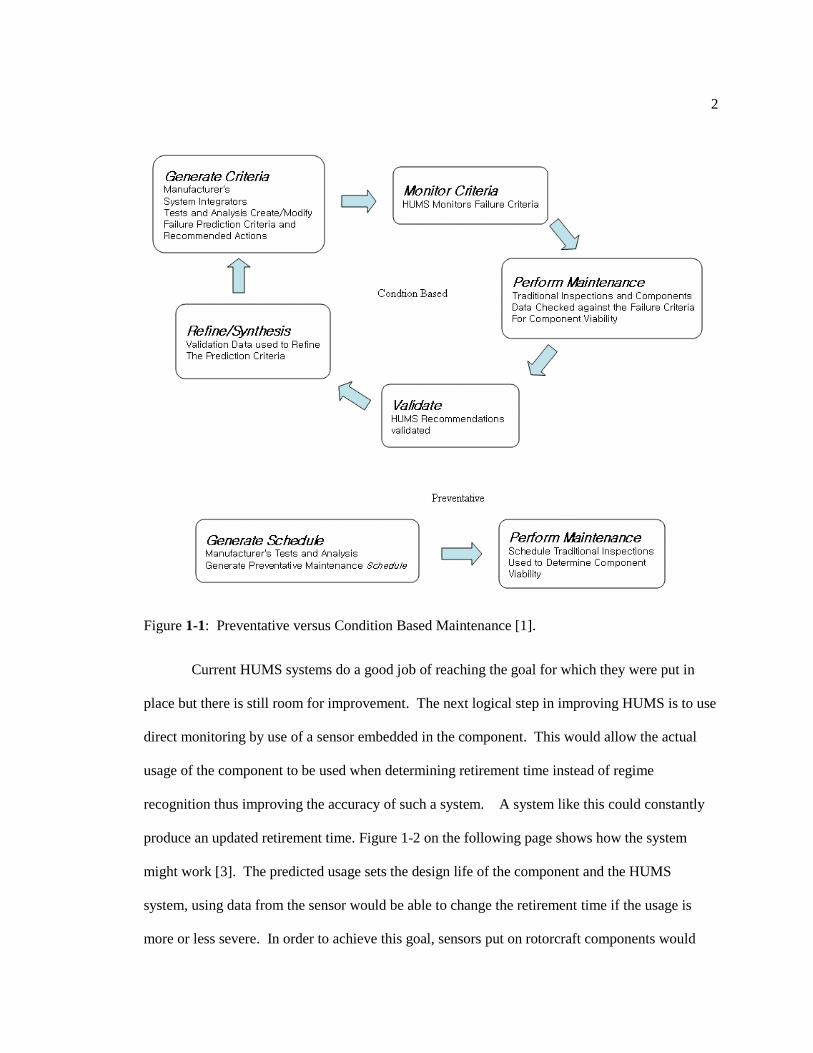
A shift to HUMS systems allows for a condition based philosophy where components are
monitored and failure is projected based on usage rather than prediction [1]. Regime recognition
says that during each flight regime the component accrues a certain amount of damage. Accurate
recognition of each regime during flight is essential to determining the total damage seen by the
component. Sometimes a pilot is asked to record the details of a flight and then regime
recognition is used to determine maintenance [2]. However, automated recording of flight
maneuvers alleviates this burden on the pilot and is more accurate. The stated goal of HUMS is
to lower maintenance cost while improving operational readiness and safety [2]. The usage
monitoring system is applied to those parts which are deemed life limited. The flowchart of
Figure 1 below shows the difference between the preventative maintenance philosophy which is
solely based on predictions and the condition based philosophy based on monitoring pre-
determined failure criteria [1].
2
Current HUMS systems do a good job of reaching the goal for which they were put in
place but there is still room for improvement. The next logical step in improving HUMS is to use
direct monitoring by use of a sensor embedded in the component. This would allow the actual
usage of the component to be used when determining retirement time instead of regime
recognition thus improving the accuracy of such a system. A system like this could constantly
produce an updated retirement time. Figure 1-2 on the following page shows how the system
might work [3]. The predicted usage sets the design life of the component and the HUMS
system, using data from the sensor would be able to change the retirement time if the usage is
more or less severe. In order to achieve this goal, sensors put on rotorcraft components would
Figure 1-1: Preventative versus Condition Based Maintenance [1].

3
need to be wireless, light weight, reliable, and powered for the entire life of the component
without adding any additional maintenance time.
Wireless sensors are already available for monitoring machinery, bridges, and other
fatigue limited structures [4]. There are also some sensors already on rotorcraft that monitor the
gearbox and other airframe components. However, the source of power for these wireless sensors
is often a battery and weight is often not a design issue due to the structures they are used on.
Batteries have a finite life and need to be replaced, making them insufficient for use in sensors on
rotary wing aircraft because they add unwanted maintenance time. A lightweight device that
harvests its own energy would never need to be replaced and can be put in locations where
battery powered devices can not.
Energy harvesting has been a major source of research in both the academic world and in
commercial industry due to its widespread potential for wireless sensor systems. Advances in
Figure 1-2: Projected Retirement Time for Condition Based Maintenance [3]. Direct monitoring
would allow the design life retirement time to be extended or shortened based on actual usage.

4
low power consumption wireless technology have increased the demand for autonomous, wireless
sensing capabilities. Batteries, for the reasons stated above, are often not desired as the main
source of power. Energy harvesting is rapidly becoming the most viable source to obtain the
power needed. There are three main ways of converting ambient mechanical energy found in the
environment into useful electrical energy. These are [5]:
1) Electromagnetic – power conversion results from the relative motion of an electrical
conductor in a magnetic field
2) Piezoelectric – use of piezoelectric materials which produce an electrical charge when
mechanically deformed
3) Electrostatic – two conductors separated by a dielectric (i.e. a capacitor). When the
conductors move, the energy stored in the capacitor changes, providing the mechanism for
conversion.
The equations governing these conversion mechanisms are discussed in detail in the next
section.
1.2 Vibration Based Energy Harvesting
Vibration based energy harvesters can be modeled as a mass-spring-damper system like
the one shown in Fig 1-3. The system consists of a seismic mass, m, a spring with stiffness k, and
a damper c. The extracted energy is represented by a damper whose force is proportional to
velocity. The operating principle is that the inertia of the mass causes it to move relative to the
frame when the frame experiences acceleration [5,7]. The displacement of the mass is then used
to generate energy by causing work to be done against a damping force f.

5
In this model, the absolute motion of the frame is given as y(t). This is the input motion
to the system and is assumed to be harmonic as y(t) = Y0cos ωt, where Y0 is the source motion
amplitude and ω is the source motion frequency. The displacement of the mass relative to the
frame is given as z(t). The absolute motion of the mass is therefore given as x(t) = y(t) + z(t). Zl
is the amplitude of mass-to-frame displacement and will be a limiting factor in generating energy
because unconstrained motion of the proof mass is almost never achievable. Zl/Y0 is the ratio of
proof mass relative amplitude to source motion amplitude and is known as the quality factor, Q.
The differential equation of motion for the proof mass is written as [6]:
)()()()( tymtkztzctzm . (1.1)
To get the transfer function from the frame motion, y(t), to the mass-to-frame motion, z(t), use the
Laplace transform to get into the s-domain and rearrange:
kcsms
ms
sY
sZ
2
2
)(
)(. (1.2)
Figure 1-3: Mass-Spring Damper Representation of Energy Harvester.

6
Dividing through by the mass, m, and substituting in the natural frequency, /n k m , and
damping, c = 2mζωn:
22
2
2)(
)(
nn ss
s
sY
sZ
. (1.3)
Divide through by ωn2 and replace s with jω. Then take the magnitude to get:
22
2
2
0
0
21
)/(
nn
n
Y
Z
. (1.4)
The energy lost per cycle is the distance integral of the damping force over a full cycle.
The force displacement curve encloses an area known as the hysteresis loop that is proportional to
the energy lost per cycle [8]. The damping force is proportional to the velocity of the proof mass,
so dF cz . Therefore, the energy harvested per cycle is:
0
0
Z
cycleZ
E c zdz
. (1.5)
The integral of (1.5) becomes:
2
0cycleE c z dt
. (1.6)
Assuming 0 sinz Z t , and the period η = 2π/ω, (1.6) becomes:
2
2 2 2
0coscycleE c Z t dt
. (1.7)
Carrying out the integral of (1.7), 2
cycleE c Z . The average power flow is defined is
/avg cycleP E where η = 2π/ω. This gives2 2 / 2avgP Z c . The ratio of source frequency, ω,
to the natural frequency of the resonant device, ωn, will be referred to as ωr. Solving equation 1.4
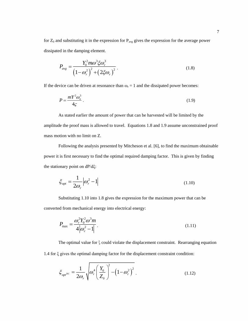
7
for Z0 and substituting it in the expression for Pavg gives the expression for the average power
dissipated in the damping element.
2 3 3
0
2 221 2
ravg
r r
Y mP
. (1.8)
If the device can be driven at resonance than ωr = 1 and the dissipated power becomes:
2 3
4
nmYP
. (1.9)
As stated earlier the amount of power that can be harvested will be limited by the
amplitude the proof mass is allowed to travel. Equations 1.8 and 1.9 assume unconstrained proof
mass motion with no limit on Z.
Following the analysis presented by Mitcheson et al. [6], to find the maximum obtainable
power it is first necessary to find the optimal required damping factor. This is given by finding
the stationary point on dP/dξ:
211
2opt r
r
(1.10)
Substituting 1.10 into 1.8 gives the expression for the maximum power that can be
converted from mechanical energy into electrical energy:
2 2 3
0max 24 1
r
c
Y mP
. (1.11)
The optimal value for ζ could violate the displacement constraint. Rearranging equation
1.4 for ξ gives the optimal damping factor for the displacement constraint condition:
2
24 20
0
11
2DC r ropt
r
Y
Z
. (1.12)

8
Substituting 1.12 into 1.8 gives the power generated when observing the displacement
constraint condition:
2 2
2 32
4 20 0 0
2max0 0
12
DC r r
r
Y m Z YP
Y Z
. (1.13)
The power, then, that can be generated at resonance (ωr = 1) is:
2 3
0 0
max02
DC
Y m ZP
Y
(1.14)
These equations do not take into account the method by which energy will be
extracted from the system. The following sections describe how the three main
mechanisms of extraction work starting with electromagnetic implementation.
1.2.1 Electromagnetic Implementation
The damping mechanism used to extract power in an electromagnetic energy harvester
will be an interaction between a moving magnet and stationary coil [5]. When the magnet is not
moving, its magnetic field creates a flux through the loop. This flux, however, is not changing
and therefore no current is induced as shown below in Fig. 1-2a. When the magnet moves into
the loop, the flux is increased. An upwards secondary magnetic field is created that opposes the
downward magnetic field as shown below in Fig 1-2b. The current in the loop must flow counter-
clockwise in order to create the secondary magnetic field.

9
When the velocity of the magnet is reversed, the secondary magnetic field changes direction to
once again oppose the motion of the magnet. This is shown in Fig 1-4c.
A model of an electromagnetic generator, where the damping mechanism for energy
extraction is an interaction between the magnet and coil is shown below in figure 1-5 [6].
Figure 1-4: Change in Magnetic Flux due to a Moving Magnet in a Coil.
Figure 1-5: Electromagnetic Energy Harvester Model [6].

10
The coil-magnet interaction described above is dependant on the properties of the
magnet and coil. The moving magnet has a magnetic flux B and the stationary coil has a
resistance Rc and inductance Lc. The coil also must be wrapped giving it two more properties; the
number of turns N, and the average length of the turn, L. The voltage generated in the coil by a
moving magnet with velocity z (t) is ( ) ( )v t NLBz t . Assuming that the magnet moves
sinusoidally with frequency ω and is connected to a resistive load RL, the current will be
/ L C Ci v R R j L . The effective damping in Equation 1.1 is then:
2
L C C
NLBc
R R j L
. (1.15)
The damping ratio is defined as / 2 nc m . This is then the electrical damping portion of
the total system damping. The remaining portion is the mechanical damping. Together,
e m total . Total system damping will have an effect on the bandwidth of the system.
Increasing the damping will reduce the peak power that can be harvested but increases the
frequency bandwidth over which power can be harvested. The equation for voltage generated in
a coil by a moving magnet assumes that the magnet is moving in the center of the coil. However,
if the magnet is not moving in the center of the coil, an efficiency term can be added so that
v t eNLBz t , where e is a number less than 1 that indicates an efficiency of less than 100%.
The e term will be looked at more closely in Section 3.5.4.
The damping coefficient, c, from equation 1.15 above can now be used in the harvester
equation of motion. Again following the analysis of Mitcheson et al. [6], substituting c into
Equation 1.1 and taking the Laplace transform gives the transfer function from base motion to
proof mass motion:

11
2
2
2
( )
( )
c L
Z s s m
Y s s NLBs m k
R R sL
. (1.16)
From here on the resistance from the coil and load will be combined into one term, R.
Substitute s = jω into equation 1.16 and collect the real and imaginary terms:
2
22 2 2 2
n n
m R j LZ
Y mR j mL NLB
. (1.17)
Taking the magnitude of equation (1.17):
2 2 2 2
0
222 2 2 2 2 2 20
n n
Z m R L
Ym R NLB mL
. (1.18)
The previous quantity is the magnitude and therefore dimensionless. The maximum
velocity of the proof mass, z(t), can be found by solving for Z in equation 1.18 and multiplying
by the frequency:
3 2 2 2
02
22 2 2 2 2 2 2
n n
Ym R LV
m R NLB mL
. (1.19)
There can now be an expression for the average power dissipated in R. It is known that
the voltage generated is ( )v NLB z t , where ( )z t is now given by V0 in equation 1.19. The
average power generated is (voltage)2/(2R) or:
22 6 2
0
4
22
22 2 2 2 2
2
1 1
n
r r
n
m Y NLB R
P
NLBR m mL
. (1.20)
The equations described in this section can now be used to design an electromagnetic energy
harvester, though more detail is still needed on the coil described in Figure 1-4 and any other
12
necessary electronics. The second method of mechanical to electrical energy conversion is
through the use of a piezoelectric material and is described in the next section
1.2.2 Piezoelectric Implementation
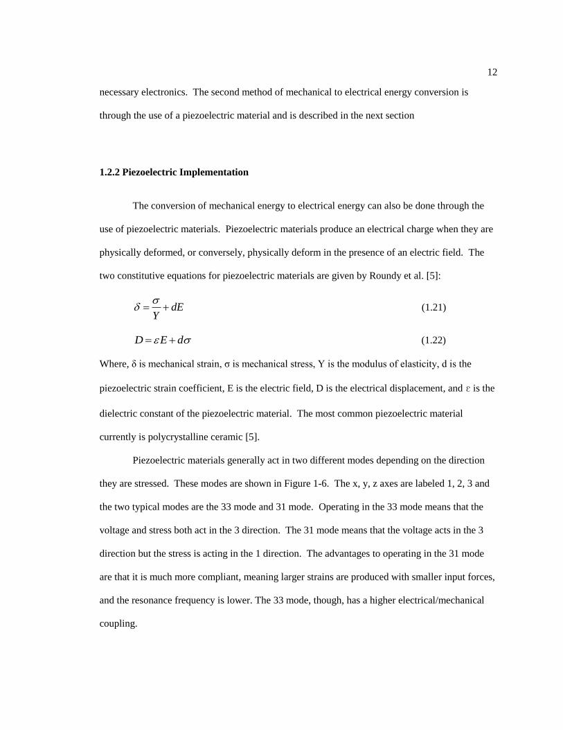
The conversion of mechanical energy to electrical energy can also be done through the
use of piezoelectric materials. Piezoelectric materials produce an electrical charge when they are
physically deformed, or conversely, physically deform in the presence of an electric field. The
two constitutive equations for piezoelectric materials are given by Roundy et al. [5]:
dEY
(1.21)
D E d (1.22)
Where, δ is mechanical strain, ζ is mechanical stress, Y is the modulus of elasticity, d is the
piezoelectric strain coefficient, E is the electric field, D is the electrical displacement, and ε is the
dielectric constant of the piezoelectric material. The most common piezoelectric material
currently is polycrystalline ceramic [5].
Piezoelectric materials generally act in two different modes depending on the direction
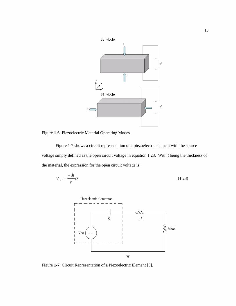
they are stressed. These modes are shown in Figure 1-6. The x, y, z axes are labeled 1, 2, 3 and
the two typical modes are the 33 mode and 31 mode. Operating in the 33 mode means that the
voltage and stress both act in the 3 direction. The 31 mode means that the voltage acts in the 3
direction but the stress is acting in the 1 direction. The advantages to operating in the 31 mode
are that it is much more compliant, meaning larger strains are produced with smaller input forces,
and the resonance frequency is lower. The 33 mode, though, has a higher electrical/mechanical
coupling.
13
Figure 1-7 shows a circuit representation of a piezoelectric element with the source
voltage simply defined as the open circuit voltage in equation 1.23. With t being the thickness of
the material, the expression for the open circuit voltage is:
OC
dtV
(1.23)
Figure 1-6: Piezoelectric Material Operating Modes.
Figure 1-7: Circuit Representation of a Piezoelectric Element [5].
14
When the piezoelectric material undergoes a periodic, sinusoidal stress due to source
vibrations, an AC voltage will appear across the load. The average power delivered to the load is
then simply P = Vload2 / 2Rload. One of the advantages of a piezoelectric device is the ability to
design it to the voltage and current that is appropriate based on the particular electrical load
circuit used. A second advantage is that no separate voltage source is needed for the initiation of
the conversion process and normally no mechanical stops are needed. This means that the
mechanical damping can be minimized.
One disadvantage of piezoelectric devices so far is its ability to be implemented on the
micro-scale level. The piezoelectric coupling gets greatly reduced at this level and has trouble
being integrated with microelectronics.
1.2.3 Electrostatic Implementation
The third and final energy conversion method is that of electrostatic conversion. This
conversion method consists of two conductors separated by a dielectric (i.e. a capacitor), which
move relative to one another. As the conductors move, the energy stored in the capacitor
changes, providing the mechanism for mechanical to electrical energy conversion. Roundy states
that the voltage across the capacitor is [5]:
0
QdV
lw . (1.24)
This equation assumes a rectangular parallel plate capacitor with length l and width w. Q is the
charge on the capacitor, d is the distance between plates and ε0 is the dielectric constant of free
space. Equation 1.24 is the same as V = Q/C, where the capacitance C is given by C = ε0lw/d.
To increase the voltage then, the capacitance should be decreased assuming the charge is held
constant. This can be accomplished by reducing l or w or increasing d. If the voltage is held

15
constant, then the charge can be increased by reducing d, or increasing l and w. Both methods
increase the energy stored on the capacitor. The conversion device is then a capacitive structure
which changes its capacitance when driven by vibrations:
221 1
2 2 2
QE QV CV
C (1.25)
Two advantages of electrostatic converters is their ability to be integrated with
microelectronics and their ability to directly generate appropriate voltages. Two disadvantages of
electrostatic converter devices is that they require a separate voltage source to initiate energy
conversion because of the capacitor, and mechanical stops are needed to ensure that the capacitor
electrodes do not come into contact and short the circuit. This also increases the mechanical
damping in the device.
1.3 Review of Existing Devices
The objective of this thesis is to develop an electromagnetic energy harvester design that
will be used to power a sensor monitoring a dynamic component on a helicopter. Therefore, the
review of existing devices has been limited to macro-scale electromagnetic harvesters and those
that have been used on rotorcraft.
One of the earliest attempts at creating an electromagnetic harvester was by Amirtharajah
and Chandrakasan (1998) [10]. Their generator consisted of a cylindrical housing with a
cylindrical mass attached to a fixed spring at one end. A permanent magnet was attached to the
bottom of the housing. The mass had a coil attached to it and was free to move vertically within
the housing as seen in Figure 1-8. The moving coil cuts the magnetic flux and in this way voltage
is generated. The proof mass was 0.5 grams and was attached to a spring with a constant of 174
N/m. It was subjected to a frequency of 94 Hz and produced a peak output voltage of 180 mV.

16
They predicted that an average of 400μW could be generated from 2 cm of movement at 2 Hz in
human powered applications.
El-Hami et al. published a paper in 2000 in which they describe a cantilever beam spring
based electromagnetic generator [11]. The cantilever beam was clamped at one end and utilized
NdFeB magnets at the free end. The coil was fixed in position between the poles of the magnets
and consisted of 27 turns of 0.2 mm diameter enameled wire. The total volume of the device was
240 mm3. It was subjected to a frequency of 322 Hz and amplitude of 25 μm. The reported
power generated was 0.53 mW.
Another cantilever beam based prototype was developed by Glynne-Jones et al (2004)
[12]. It was also a four magnet, fixed coil arrangement. The total volume of the device was 3.15
cm3. It was subjected to a frequency of 106 Hz and an acceleration level of 2.6 m/s
2. It produced
an output voltage of 1 V. It was then mounted on a car engine and driven for 1.24 Km. The peak
power produced was 4 mW, but the average power produced was 157 μW.
Beeby et al. developed their own cantilever beam prototype in 2007 shown in Figure 1-
9. The total device volume was 150 mm3. It was subjected to an acceleration level of 0.59 m/s
2
and had a natural frequency of 52 Hz. It generated 428 mV and 46 μW of power.
Figure 1-8: Amirtharajah and Chandrakasan’s Linear Electromagnetic Harvester [10].

17
Yuan et al (2007) designed a harvester that consisted of an electroplated copper spring
released from a substrate onto which an NdFeB magnet is attached with a mass of 192 mg. The
spring mass assembly was located within a conventionally wound coil. It experienced and
acceleration level of 4.63 m/s2 and generated 120 μW [17].
Hadas et al developed a harvester as part of a European project concerned with wireless
aircraft monitoring. The volume of their device was 45 cm3 and had a natural frequency of 34.5
Hz. The acceleration level was 3.1 m/s2 and the reported power generated was 3.5 mW [18].
A human powered generator was developed by von Buren and Troster (2007) [19]. Their
design consisted of a tubular translator containing a number of cylindrical magnets separated by
spacers. The translator moves vertically within a series of stator coils with the vertical motion
being controlled by a parallel spring stage consisting of two parallel beams. The stator and
translator designs were realized with six magnets and five coils and had a total volume of 30.4
cm3. The reported average power output was 35 μW. A good table of existing commercial
devices can be found in Priya and Inman’s “Energy Harvesting Technologies” [9].
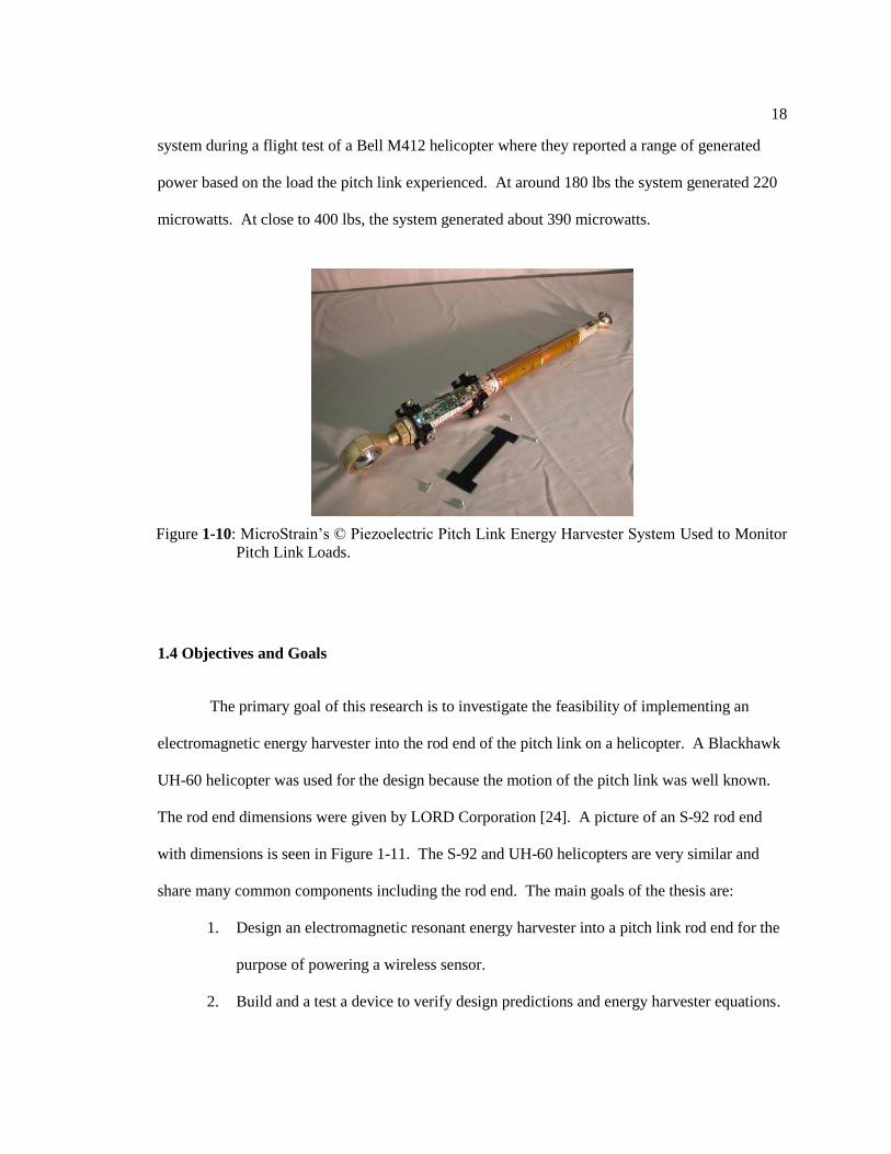
One attempt at harvesting energy from a helicopter pitch link came from MicroStrain’s ©
piezoelectric based harvester [20], [21], [22], [23]. They attempted to place piezoelectric
elements along the outside of the pitch link which is subjected to + 35 microstrain at 5 Hz. The
total weight of the system was about 116 grams. MicroStrain© successfully demonstrated their
Figure 1-9: Beeby et al’s Cantilever Beam Configuration [12].
18
system during a flight test of a Bell M412 helicopter where they reported a range of generated
power based on the load the pitch link experienced. At around 180 lbs the system generated 220
microwatts. At close to 400 lbs, the system generated about 390 microwatts.
1.4 Objectives and Goals
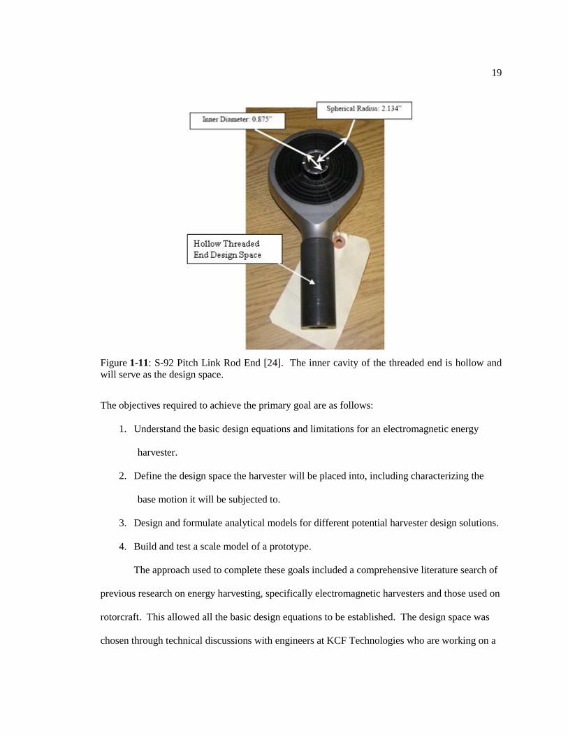
The primary goal of this research is to investigate the feasibility of implementing an
electromagnetic energy harvester into the rod end of the pitch link on a helicopter. A Blackhawk
UH-60 helicopter was used for the design because the motion of the pitch link was well known.
The rod end dimensions were given by LORD Corporation [24]. A picture of an S-92 rod end
with dimensions is seen in Figure 1-11. The S-92 and UH-60 helicopters are very similar and
share many common components including the rod end. The main goals of the thesis are:
1. Design an electromagnetic resonant energy harvester into a pitch link rod end for the
purpose of powering a wireless sensor.
2. Build and a test a device to verify design predictions and energy harvester equations.
Figure 1-10: MicroStrain’s © Piezoelectric Pitch Link Energy Harvester System Used to Monitor
Pitch Link Loads.
19
The objectives required to achieve the primary goal are as follows:
1. Understand the basic design equations and limitations for an electromagnetic energy
harvester.
2. Define the design space the harvester will be placed into, including characterizing the
base motion it will be subjected to.
3. Design and formulate analytical models for different potential harvester design solutions.
4. Build and test a scale model of a prototype.
The approach used to complete these goals included a comprehensive literature search of
previous research on energy harvesting, specifically electromagnetic harvesters and those used on
rotorcraft. This allowed all the basic design equations to be established. The design space was
chosen through technical discussions with engineers at KCF Technologies who are working on a
Figure 1-11: S-92 Pitch Link Rod End [24]. The inner cavity of the threaded end is hollow and
will serve as the design space.

20
similar problem and have talked to experts in the helicopter industry. The pitch link rod end
motion was characterized through computer simulations performed at Penn State’s Rotorcraft
Center.
This thesis outlines the design process for designing an electromagnetic energy harvester
into a pitch link rod end with the goal of powering a sensor. A design was chosen and then tested
on a system that mimics the motion of the pitch link during different flight conditions. Two
different harvesters were tested to characterize performance parameters and to correlate with the
analytical models used for design simulations and performance assessments. The two harvesters
were based on the same design concept.

Chapter 2
Design of a New Energy Harvesting Device
Designs for an electromagnetic energy harvester in the rod end of a pitch link were
explored. The forces acting on the proof mass in the harvester were first examined. The effects
of four main parameters related to the available power were then looked at in detail, namely mass,
frequency, damping, and quality factor. Three different designs were explored and considered for
testing. For all designs, an analytical model was developed to look at the dynamics of the design,
and theoretical available power is discussed. Finally, the magnet and electromagnetic coil design
and interaction were detailed and discussed.
2.1 Pitch Link Rod End Dynamic Environment
The first step in designing an energy harvester is to accurately characterize the
environment it will be expected to operate in. A MATLAB script computer code written at Penn
State’s Rotorcraft Center was used to describe the motion of the pitch link at a variety of flight
conditions [25]. The script calculates the time history of the pitch link during one revolution
based on user input of collective and cyclic pitch. Collective and cyclic pitches are two controls
that pilots use to control the flight path of the helicopter. The cyclic pitch control changes the
pitch of the rotor blades depending on their position as they rotate around the hub so that all
blades change their angle by the same amount in the same point in the cycle. The collective pitch
changes the pitch angle of all the main rotor blades at the same time independent of their position.
A diagram of the pitch link and swash plate is shown below in Figure 2-1. In the diagram CPL is
the length of the pitch link, rp is the vector to the base of the pitch link, rh is the vector from the

22
root of the blade along the pitch horn to the pitch link, and rb is the vector from the center of the
swash plate to the root of the blade.
An example output of the analysis is shown below for 5o cyclic and 18
o collective. This
is the vertical motion of the pitch link in meters for this particular flight condition. The frequency
of the motion of the pitch link is 4.3 Hz corresponding to the main rotor rotational speed. This is
constant for the duration of the flight.
Figure 2-1: Diagram of Pitch Link and Swash Plate with Vectors [25].
0 0.2 0.4 0.6 0.8 1 1.2 1.4 1.6 1.8 2-0.015
-0.01
-0.005
0
0.005
0.01
0.015Vertical Motion of Pitch Link
Time (sec)
Vert
ical P
ositio
n (
m)
Figure 2-2: Time History of Vertical Motion of Pitch Link for 5 degree cyclic input.
23
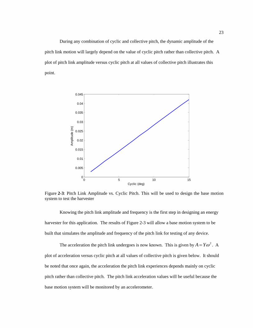
During any combination of cyclic and collective pitch, the dynamic amplitude of the
pitch link motion will largely depend on the value of cyclic pitch rather than collective pitch. A
plot of pitch link amplitude versus cyclic pitch at all values of collective pitch illustrates this
point.
Knowing the pitch link amplitude and frequency is the first step in designing an energy
harvester for this application. The results of Figure 2-3 will allow a base motion system to be
built that simulates the amplitude and frequency of the pitch link for testing of any device.
The acceleration the pitch link undergoes is now known. This is given by2A Y . A
plot of acceleration versus cyclic pitch at all values of collective pitch is given below. It should
be noted that once again, the acceleration the pitch link experiences depends mainly on cyclic
pitch rather than collective pitch. The pitch link acceleration values will be useful because the
base motion system will be monitored by an accelerometer.
0 5 10 150
0.005
0.01
0.015
0.02
0.025
0.03
0.035
0.04
0.045
Cyclic (deg)
Am
plit
ude (
m)
Figure 2-3: Pitch Link Amplitude vs. Cyclic Pitch. This will be used to design the base motion
system to test the harvester

24
The pitch link, however, does not have purely vertical motion. During one revolution, it
also has a small angular component that can be seen from Figure 2-1. This is also dependent on
the values of cyclic and collective pitch. Seen below in Figure 2-5 is the angular movement of
the pitch link at 5o cyclic and 18
o collective.
0 5 10 150
5
10
15
20
25
30
35
Cyclic (deg)
Accele
ration (
m/s
2)
Figure 2-4: Pitch Link Acceleration vs. Cyclic Pitch. This is another way of looking at the base
motion and will be useful when monitoring with an accelerometer
0 0.2 0.4 0.6 0.8 1 1.2 1.4 1.6 1.8 2
0.2
0.25
0.3
0.35
0.4
0.45
0.5
0.55
0.6
0.65Pitch Link Angle
Angle
(degre
es)
Time (sec)
Figure 2-5: Angular Movement of Pitch Link.

25
Given a certain device, the angular movement of the pitch link can have an affect on the
magnitude and direction of the centrifugal force. This will be looked at in Section 2.1.1. The
motion of the pitch link at all values of cyclic and collective pitch are now known and
understood. When designing the harvester, it will be very important to know the forces acting on
the proof mass in order to design an optimized resonant system.
2.1.1 Influence of Centrifugal Forces
The pitch link is located away from the center of rotation of the shaft that spins the blades
as seen in Figure 2-6. Therefore, any mass placed inside the pitch link will experience centrifugal
forces proportional to its mass. The centrifugal force is2F m r , where m is the mass, ω is the
rotational speed, and r is the distance from the center of rotation. The value of r is given as 0.41
meters for a UH-60 helicopter and ω is known to be 27.02 rad/s. A graph of the centrifugal force
versus mass is given in Figure 2-7 for masses from 2 grams to 20 grams.
Figure 2-6: Pitch Link Location on the HUB. r is the distance from the main rotor shaft to the
pitch link.

26
If the mass is allowed to stay in-line with the pitch link during the duration of its travel,
then it will experience a centrifugal force in both the horizontal and vertical directions when the
pitch link is tilted at the angle described in Section 2-1. A diagram of the centrifugal forces in
this situation is shown below.
0
1
2
3
4
5
6
7
0 5 10 15 20 25
Mass (g)
CF (
N)
Figure 2-7: Mass versus Centrifugal Force Showing how CF will Increase with Proof Mass.
Figure 2-8: Centrifugal Forces when Pitch Link is at an Angle.
27
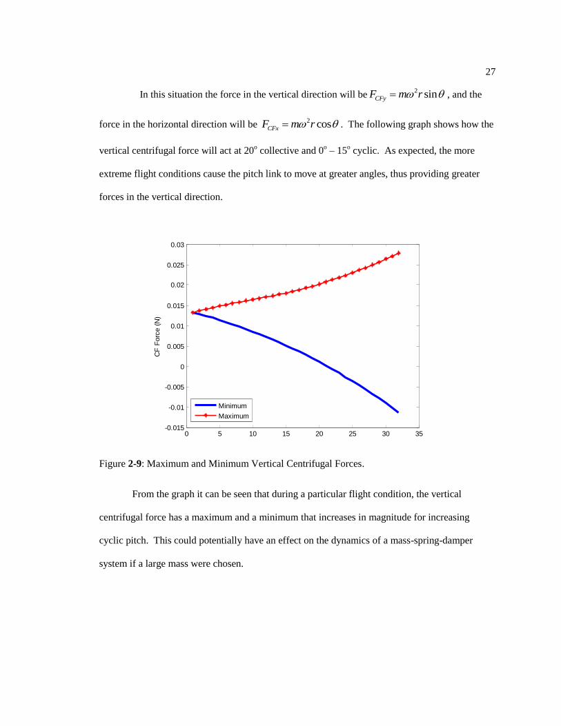
In this situation the force in the vertical direction will be2 sinCFyF m r , and the
force in the horizontal direction will be 2 cosCFxF m r . The following graph shows how the
vertical centrifugal force will act at 20o collective and 0
o – 15
o cyclic. As expected, the more
extreme flight conditions cause the pitch link to move at greater angles, thus providing greater
forces in the vertical direction.
From the graph it can be seen that during a particular flight condition, the vertical
centrifugal force has a maximum and a minimum that increases in magnitude for increasing
cyclic pitch. This could potentially have an effect on the dynamics of a mass-spring-damper
system if a large mass were chosen.
0 5 10 15 20 25 30 35-0.015
-0.01
-0.005
0
0.005
0.01
0.015
0.02
0.025
0.03
CF
Forc
e (
N)
Minimum
Maximum
Figure 2-9: Maximum and Minimum Vertical Centrifugal Forces.

28
2.1.2 Geometric Constraints
The harvester will be placed in the rod end of the pitch link as stated in Chapter 1. This
design space provides the geometric constraints of the device that will limit mass size and motion
and coil size. The effects that these will have on the available power will be discussed in the
upcoming sections. The rod end that the device will be designed to fit into can be seen in Figure
1-11 of Section 1.4. The inner diameter of the rod end in 0.75 inches (19.05 mm) and its length is
4 inches (101.6 mm) [25]. These dimensions can be seen below in Figure 2-10.
2.2 Available Power
The equations derived in Chapter 1 can be used to predict the amount of available power
the system has. This available power is dependent on four main parameters; mass of the system,
frequency of the source, system damping, and quality factor, which refers to the ratio of source
Figure 2-10: S-92 Pitch Link Rod End Inside Dimensions [25]. The harvester will go inside the
cavity shown in the picture.

29
motion amplitude to system motion amplitude. Three of these parameters, mass, damping, and
quality factor, can be controlled by the designer within the design space, whereas the third
parameter, frequency of the source, cannot be controlled by the designer. The following four
sections attempt to better understand the effect these four system parameters will have on the
available power for harvesting.
2.2.1 Effect of Mass on Available Power
The available power equation (equation 1.8) from Chapter 1 is restated here and will be
referred to as the average power equation from here on:
2 3 3
0
2 221 2
ravg
r r
Y mP
(1.8)
Also from Chapter 1 (equation 1.9), the average power dissipated when the natural frequency of
the device matches the natural frequency of the source is the matched average power::
2 3
4
mYP
(1.9)
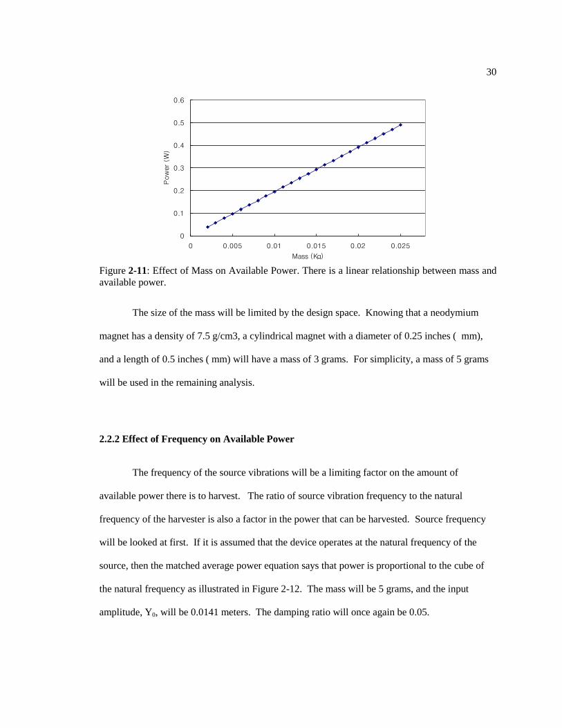
It is obvious here that power will be directly proportional to mass and that the greater
mass the system has the more power that will be available. This simple relationship is shown
graphically below for different values of mass. It is assumed here that the device natural
frequency matches the driving natural frequency so ωr = 1. The frequency is again taken as 27.02
rad/s. Y0 will be taken as 0.0141 meters which is a nominal flight condition corresponding to 5o
cyclic, and ζ will be 0.05. The figure illustrates the point that if the frequency can be matched
then the amount of energy there is to harvest will increase linearly with increasing mass.
30
The size of the mass will be limited by the design space. Knowing that a neodymium
magnet has a density of 7.5 g/cm3, a cylindrical magnet with a diameter of 0.25 inches ( mm),
and a length of 0.5 inches ( mm) will have a mass of 3 grams. For simplicity, a mass of 5 grams
will be used in the remaining analysis.
2.2.2 Effect of Frequency on Available Power
The frequency of the source vibrations will be a limiting factor on the amount of
available power there is to harvest. The ratio of source vibration frequency to the natural
frequency of the harvester is also a factor in the power that can be harvested. Source frequency
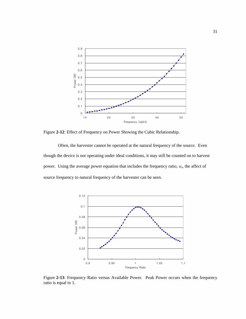
will be looked at first. If it is assumed that the device operates at the natural frequency of the
source, then the matched average power equation says that power is proportional to the cube of
the natural frequency as illustrated in Figure 2-12. The mass will be 5 grams, and the input
amplitude, Y0, will be 0.0141 meters. The damping ratio will once again be 0.05.
Mass vs. Power
0
0.1
0.2
0.3
0.4
0.5
0.6
0 0.005 0.01 0.015 0.02 0.025
Mass (Kg)
Pow
er (W
)
Figure 2-11: Effect of Mass on Available Power. There is a linear relationship between mass and
available power.
31
Often, the harvester cannot be operated at the natural frequency of the source. Even
though the device is not operating under ideal conditions, it may still be counted on to harvest
power. Using the average power equation that includes the frequency ratio, ωr, the affect of
source frequency to natural frequency of the harvester can be seen.
0
0.1
0.2
0.3
0.4
0.5
0.6
0.7
0.8
0.9
14 24 34 44 54
Frequency (rad/s)
Pow
er (W
)
Figure 2-12: Effect of Frequency on Power Showing the Cubic Relationship.
0
0.02
0.04
0.06
0.08
0.1
0.12
0.9 0.95 1 1.05 1.1
Frequency Ratio
Pow
er (W
)
Figure 2-13: Frequency Ratio versus Available Power. Peak Power occurs when the frequency
ratio is equal to 1.
32
As expected, the peak power is generated when the driving frequency matches the natural
frequency of the harvester. At this point, a resonating harvester has the most available kinetic
energy to harvest. In the next section, the affect that damping has on the curve of Figure 2-13
will be examined.
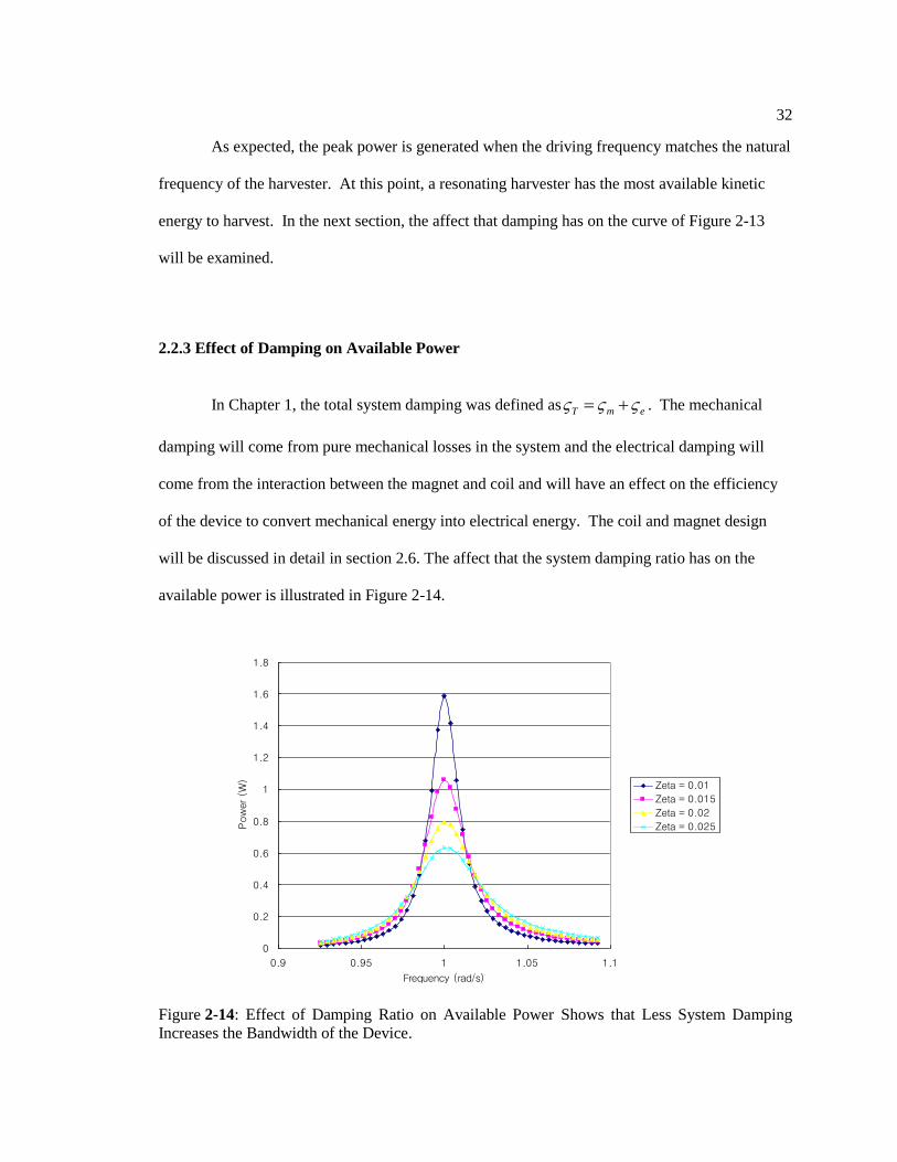
2.2.3 Effect of Damping on Available Power
In Chapter 1, the total system damping was defined as T m e . The mechanical
damping will come from pure mechanical losses in the system and the electrical damping will
come from the interaction between the magnet and coil and will have an effect on the efficiency
of the device to convert mechanical energy into electrical energy. The coil and magnet design
will be discussed in detail in section 2.6. The affect that the system damping ratio has on the
available power is illustrated in Figure 2-14.
0
0.2
0.4
0.6
0.8
1
1.2
1.4
1.6
1.8
0.9 0.95 1 1.05 1.1
Frequency (rad/s)
Pow
er (W
)
Zeta = 0.01
Zeta = 0.015
Zeta = 0.02
Zeta = 0.025
Figure 2-14: Effect of Damping Ratio on Available Power Shows that Less System Damping
Increases the Bandwidth of the Device.
33
The results of Figure 2-14 assume that the mechanical damping equals the electrical
damping. It clearly shows that the damping ratio will have a great effect on the power that is
harvested. For less damping, there is more power available but a greater price is paid if the
frequency ratio does not equal 1. Conversely, the more damping the system has, the less overall
power there is to harvest, but the bandwidth of the system is greater and thus less of a penalty is
paid when the frequency ratio is not equal to one. The type of damping however, will also affect
how much power is harvested.
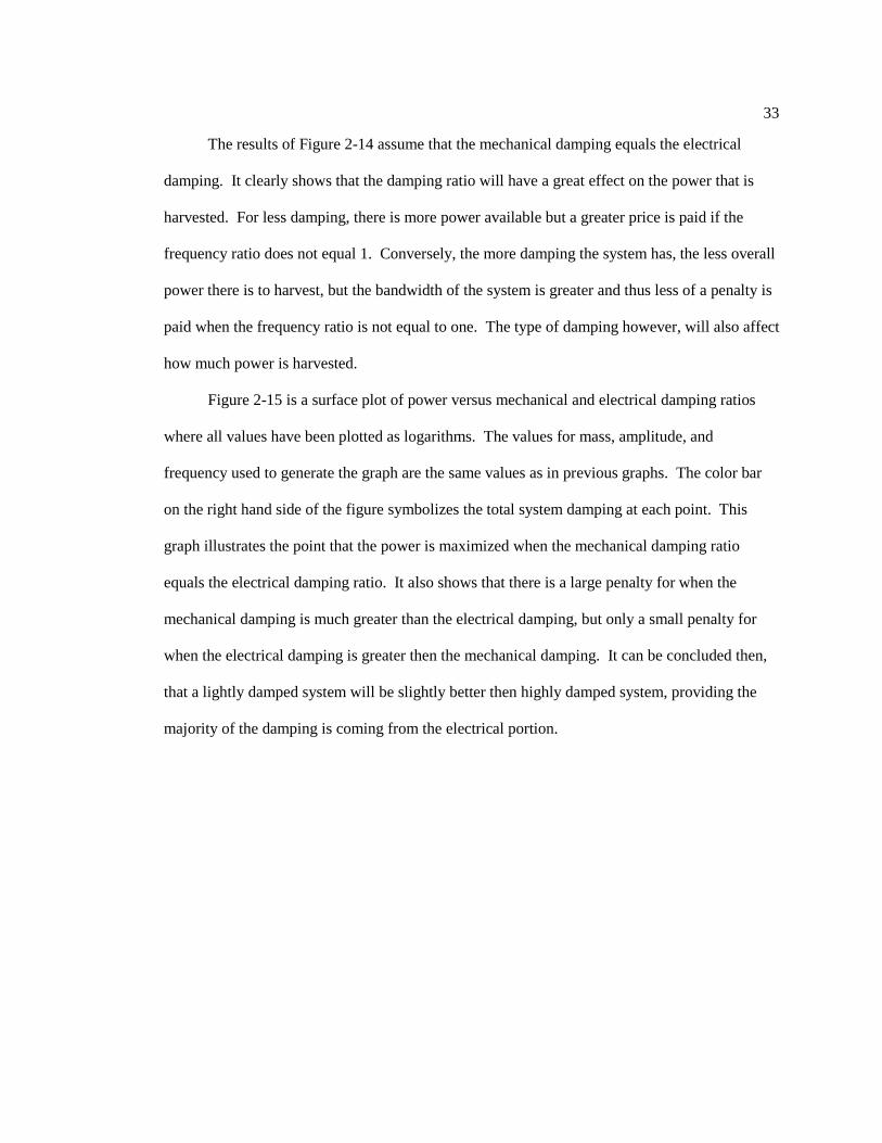
Figure 2-15 is a surface plot of power versus mechanical and electrical damping ratios
where all values have been plotted as logarithms. The values for mass, amplitude, and
frequency used to generate the graph are the same values as in previous graphs. The color bar
on the right hand side of the figure symbolizes the total system damping at each point. This
graph illustrates the point that the power is maximized when the mechanical damping ratio
equals the electrical damping ratio. It also shows that there is a large penalty for when the
mechanical damping is much greater than the electrical damping, but only a small penalty for
when the electrical damping is greater then the mechanical damping. It can be concluded then,
that a lightly damped system will be slightly better then highly damped system, providing the
majority of the damping is coming from the electrical portion.
34
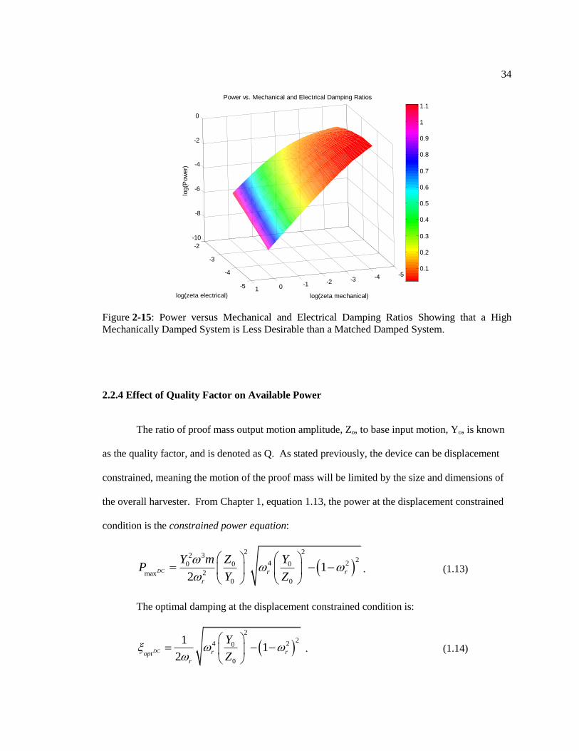
2.2.4 Effect of Quality Factor on Available Power
The ratio of proof mass output motion amplitude, Zo, to base input motion, Yo, is known
as the quality factor, and is denoted as Q. As stated previously, the device can be displacement
constrained, meaning the motion of the proof mass will be limited by the size and dimensions of
the overall harvester. From Chapter 1, equation 1.13, the power at the displacement constrained
condition is the constrained power equation:
2 2
2 32
4 20 0 0
2max0 0
12
DC r r
r
Y m Z YP
Y Z
. (1.13)
The optimal damping at the displacement constrained condition is:
2
24 20
0
11
2DC r ropt
r
Y
Z
. (1.14)
-5
-4
-3
-2
-5-4-3-2-101
-10
-8
-6
-4
-2
0
log(zeta mechanical)
Power vs. Mechanical and Electrical Damping Ratios
log(zeta electrical)
log(P
ow
er)
0.1
0.2
0.3
0.4
0.5
0.6
0.7
0.8
0.9
1
1.1
Figure 2-15: Power versus Mechanical and Electrical Damping Ratios Showing that a High
Mechanically Damped System is Less Desirable than a Matched Damped System.

35
Figure 2-16 is a surface plot of quality factor, (Zl/Y0) and frequency ratio versus power. The
color bar on the right represents the total system damping at each point.
As expected, the most power is generated when the frequency ratio is equal to one and
the quality factor is at its highest. A quality factor of 10 to 1 may be very difficult to achieve
however. Also, the damping has been re-optimized at each point on the graph. This is very
difficult to do mechanically, but can be more easily done by adjusting the load electronics [5].
2.3 Linear Harvester Design
The first design is that of a linear harvester. In this design, the magnet acts as the proof
mass and is connected to a linear spring. In order to resist the lateral centrifugal force, the mass is
on a low friction bearing that will still allow motion in the vertical direction. In this
configuration, the coil would have to be placed near the magnet instead of around it. Also, in this
design the vertical centrifugal forces will come into play, as the magnet will always be in line
02
46
810
0.9
0.95
1
1.05
1.1
0
0.1
0.2
0.3
0.4
Zl/Yowr (w/wn)
Pow
er
(W)
0
0.05
0.1
0.15
0.2
0.25
0.3
0.35
0.4
0.45
0.5
Figure 2-16: Quality Factor and Frequency Ratio versus Power. This shows that a high quality
factor and frequency matching will have the most available power.

36
with the pitch link which moves angularly, as well as vertically, as described in Sections 2.1 and
2.11. The biggest challenge in implementing this design, as it will be in all of the designs, is to
control the amplitude of the proof mass at all of the different flight conditions and still harvest the
required power. Figure 2-17 below offers a very simple schematic of what the device might look
like.
The equations of motion for this system are the same as for the harvester described in
Section 1.2 and for Figure 1-1. The base motion consists of the vertical acceleration from the
pitch link and also the time varying vertical centrifugal forces that will accelerate the proof mass.
A MATLAB script and a Simulink model have been implemented to simulate the motion of a
device like this at all the different flight conditions that it will experience. A plot of the motion of
the proof mass when the helicopter is flying at 20o collective and 4
o cyclic is seen below in Figure
2-18. The system takes on a dramatically different response with the added effect of the
centrifugal forces.
Figure 2-17: Linear Harvester Design. In this design a magnet is attached to a linear spring
vibrating next to a stationary coil.
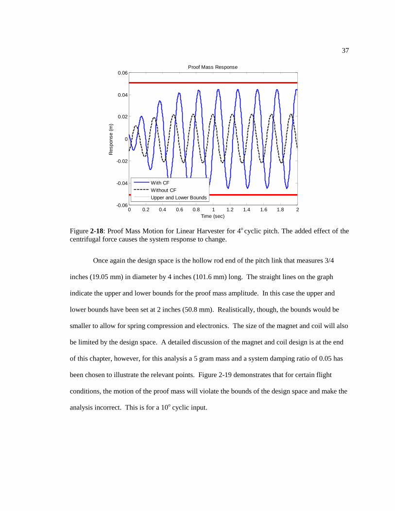
37
Once again the design space is the hollow rod end of the pitch link that measures 3/4
inches (19.05 mm) in diameter by 4 inches (101.6 mm) long. The straight lines on the graph
indicate the upper and lower bounds for the proof mass amplitude. In this case the upper and
lower bounds have been set at 2 inches (50.8 mm). Realistically, though, the bounds would be
smaller to allow for spring compression and electronics. The size of the magnet and coil will also
be limited by the design space. A detailed discussion of the magnet and coil design is at the end
of this chapter, however, for this analysis a 5 gram mass and a system damping ratio of 0.05 has
been chosen to illustrate the relevant points. Figure 2-19 demonstrates that for certain flight
conditions, the motion of the proof mass will violate the bounds of the design space and make the
analysis incorrect. This is for a 10o cyclic input.
0 0.2 0.4 0.6 0.8 1 1.2 1.4 1.6 1.8 2-0.06
-0.04
-0.02
0
0.02
0.04
0.06Proof Mass Response
Time (sec)
Response (
m)
With CF
Without CF
Upper and Lower Bounds
Figure 2-18: Proof Mass Motion for Linear Harvester for 4o cyclic pitch. The added effect of the
centrifugal force causes the system response to change.
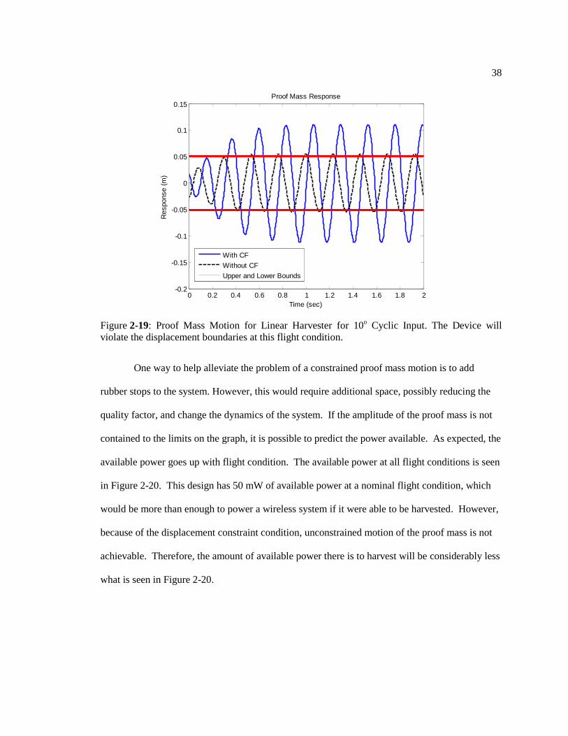
38
One way to help alleviate the problem of a constrained proof mass motion is to add
rubber stops to the system. However, this would require additional space, possibly reducing the
quality factor, and change the dynamics of the system. If the amplitude of the proof mass is not
contained to the limits on the graph, it is possible to predict the power available. As expected, the
available power goes up with flight condition. The available power at all flight conditions is seen
in Figure 2-20. This design has 50 mW of available power at a nominal flight condition, which
would be more than enough to power a wireless system if it were able to be harvested. However,
because of the displacement constraint condition, unconstrained motion of the proof mass is not
achievable. Therefore, the amount of available power there is to harvest will be considerably less
what is seen in Figure 2-20.
0 0.2 0.4 0.6 0.8 1 1.2 1.4 1.6 1.8 2-0.2
-0.15
-0.1
-0.05
0
0.05
0.1
0.15Proof Mass Response
Time (sec)
Response (
m)
With CF
Without CF
Upper and Lower Bounds
Figure 2-19: Proof Mass Motion for Linear Harvester for 10o Cyclic Input. The Device will
violate the displacement boundaries at this flight condition.
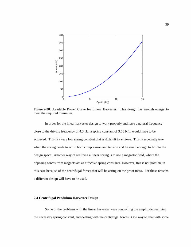
39
In order for the linear harvester design to work properly and have a natural frequency
close to the driving frequency of 4.3 Hz, a spring constant of 3.65 N/m would have to be
achieved. This is a very low spring constant that is difficult to achieve. This is especially true
when the spring needs to act in both compression and tension and be small enough to fit into the
design space. Another way of realizing a linear spring is to use a magnetic field, where the
opposing forces from magnets act as effective spring constants. However, this is not possible in
this case because of the centrifugal forces that will be acting on the proof mass. For these reasons
a different design will have to be used.
2.4 Centrifugal Pendulum Harvester Design
Some of the problems with the linear harvester were controlling the amplitude, realizing
the necessary spring constant, and dealing with the centrifugal forces. One way to deal with some
0 5 10 150
50
100
150
200
250
300
350
400
Cyclic (deg)
Pow
er
(mW
)
Figure 2-20: Available Power Curve for Linear Harvester. This design has enough energy to
meet the required minimum.

40
of these problems is to use the centrifugal force as the effective spring instead of relying on a
mechanical spring. This can be achieved by a centrifugal pendulum in which the proof mass is
hinged on the inside wall of the rod end and the mass is placed in line with the centrifugal force.
The hinge would alleviate the need to deal with the angular movement of the pitch link. A free
body diagram of a system like this is in Figure 2-21.
The dynamics of this system are similar to that of the linear harvester if we assume small
amplitudes and linear motion of the proof mass. The distance e is the distance from the rotating
shaft to the pitch link and r is the distance from the rotating shaft to proof mass. Using the small
angle assumption, z = (r-e)β and z(t) = x(t) – y(t). The following table summarizes the forces
acting on the proof mass and each of their arms. CF stands for centrifugal force, IF stands for
inertial force, and Fd is the damping force.
Figure 2-21: Free Body Diagram of a Centrifugal Pendulum Harvester that uses the Centrifugal
Force as an Effective Spring.

41
Summing forces on the mass about the hinge, the differential equation of motion for the
device is:
2 0hingeM m r e x D r e z m rz . (2.1)
Substituting in the expression for x(t):
2m r e z D r e z m rz m r e y . (2.2)
Dividing through by m(r-e) we get the differential equation of motion for the centrifugal
pendulum where the constant in front of the z term represents the stiffness of the system due to
the centrifugal force.
2D rz z z y
m r e
. (2.3)
Taking the Laplace transform and re-arranging gives the transfer function in the s-domain
from base input motion Y, to proof mass output motion Z, with the centrifugal force providing the
system stiffness.
2
22
( )
( )
Z s s
D rY ss s
m r e
. (2.4)
It is known that 2 nD m where m is the proof mass, ωn is the natural frequency of the
system, and ζ is total system damping, both mechanical and electrical. Substituting into the
Table 2-1: Forces acting on Centrifugal Pendulum Harvester Proof Mass.
Force Arm
CF:
IF:
Fd:
2m r
mx m z y
z
r e
r eDz

42
above transfer function and also naming the stiffness term, k, we again get the transfer function
from input motion to output motion:
2
2
( )
( ) 2 n
Z s s
Y s s s k
. (2.5)
If e were much less than r, than the stiffness term k would go closer to Ω2 and the natural
frequency of the system would be proportional to the rotational speed of the rotor. If this were
true than the system would always be tuned close to 1/rev. However, e is not much less than r
and the systems natural frequency is not tuned to the rotational speed of the rotor. This transfer
function was once again implemented in Simulink and the parameters of it were defined in a
MATLAB script. The diagram of the Simulink model is in Figure 2-22 where the base motion
from the pitch link is fed into the transfer function.
The motion of the proof mass at 20o collective and 10
o cyclic is used as an example in
Figure 2-23. At this flight condition the pitch link experiences an acceleration of 20.59 m/s2. The
values used in the simulation were a 5 gram mass, a driving frequency of 27 rad/s, a total system
damping ratio of 0.05, r equal to 0.42m, and e equal to 0.41m.
-s 2
s +D.s+k2
Transfer Fcn
signal
To Workspace2
time
To Workspace1
Z
To Workspace
[time signal]
From
Workspace
Clock
Figure 2-22: Simulink Model for Centrifugal Pendulum Harvester.
43
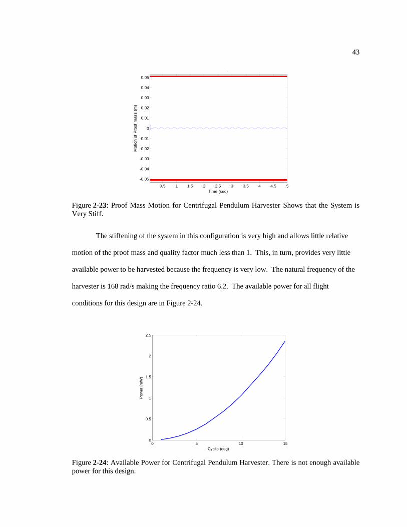
The stiffening of the system in this configuration is very high and allows little relative
motion of the proof mass and quality factor much less than 1. This, in turn, provides very little
available power to be harvested because the frequency is very low. The natural frequency of the
harvester is 168 rad/s making the frequency ratio 6.2. The available power for all flight
conditions for this design are in Figure 2-24.
0.5 1 1.5 2 2.5 3 3.5 4 4.5 5
-0.05
-0.04
-0.03
-0.02
-0.01
0
0.01
0.02
0.03
0.04
0.05
Proof Mass Response
Time (sec)
Motion o
f P
roof
mass (
m)
Figure 2-23: Proof Mass Motion for Centrifugal Pendulum Harvester Shows that the System is
Very Stiff.
0 5 10 150
0.5
1
1.5
2
2.5
Cyclic (deg)
Pow
er
(mW
)
Figure 2-24: Available Power for Centrifugal Pendulum Harvester. There is not enough available
power for this design.

44
From the figure it is obvious that there is not enough available power at most flight
conditions to power a wireless sensor. This would be expected due to the low quality factor and
off resonance frequency. Therefore, the major drawback of this configuration is that it is too stiff
to allow the needed amplitude and quality factor necessary to meet the power requirements. It
also has a natural frequency much higher than the driving frequency. It does however, offer very
little mechanical damping and uses the centrifugal force to its advantage instead of having
mechanical losses in a bearing system. The next design which is very similar in nature, addresses
these issues to allow better response from the system.
2.5 Reverse Centrifugal Pendulum Harvester Design
The issues of the previous design can be overcome by mounting the hinge of the
pendulum on the reverse side of the rod end, still keeping the proof mass in line with the
centrifugal forces. This design will have a torsional spring at the hinge that will allow the system
to be tuned based on the choice of m and k. How this will be accomplished will be shown later.
A free body diagram of this system is shown in Figure 2-25.
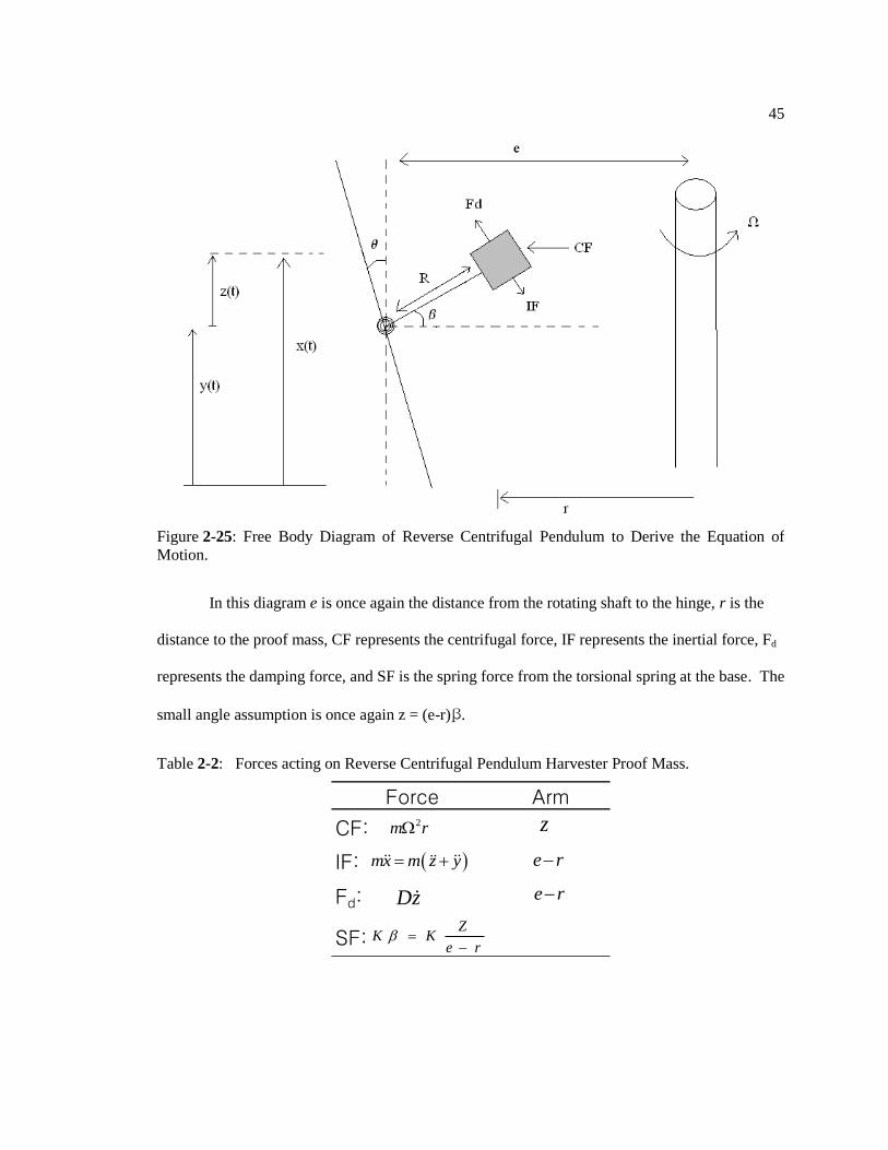
45
In this diagram e is once again the distance from the rotating shaft to the hinge, r is the
distance to the proof mass, CF represents the centrifugal force, IF represents the inertial force, Fd
represents the damping force, and SF is the spring force from the torsional spring at the base. The
small angle assumption is once again z = (e-r)β.
Figure 2-25: Free Body Diagram of Reverse Centrifugal Pendulum to Derive the Equation of
Motion.
Table 2-2: Forces acting on Reverse Centrifugal Pendulum Harvester Proof Mass.
Force Arm
CF:
IF:
Fd:
SF:
2m r
mx m z y
z
e r
e rDz
ZK K
e r

46
To get the differential equation of motion for the system, first sum moments about the
hinge:
2 0hinge tor
zM m e r x D e r z K m rz
e r
. (2.6)
Substitute in x = z + y to get the equation in terms of input and output motions.
2
tor
zm e r z D e r z K m rz m e r y
e r
. (2.7)
Dividing through by m(e-r) gives the equation of motion for the reverse centrifugal
pendulum:
2
2
torKD rz z z y
m e rm e r
. (2.8)
To get the transfer function from input motion to output motion, take the Laplace transform of the
above differential equation and rearrange:
2
22
2
( )
( )tor
Z s s
Y s KD rs s
m e rm e r
. (2.9)
Once again knowing that 2 nD m and the stiffness term, k, is once again the constant in front
of the z term in the differential equation above, the transfer function can be written:
2
2
( )
( ) 2 n
Z s s
Y s s s k
. (2.10)
This is the same transfer function as for the centrifugal pendulum harvester described in
Section 2.4 with the key difference being the stiffness term k. Comparing the stiffness terms, it
can be seen that the centrifugal pendulum gets its stiffness entirely from the centrifugal force and
choice of mass. The reverse centrifugal pendulum system is actually softened by the centrifugal
force term. It, therefore, can be tuned based on the choice for the torsional spring constant.
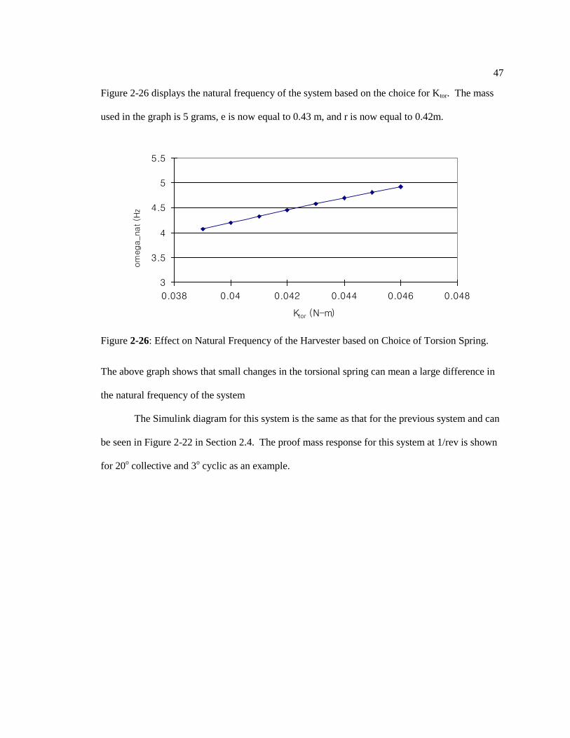
47
Figure 2-26 displays the natural frequency of the system based on the choice for Ktor. The mass
used in the graph is 5 grams, e is now equal to 0.43 m, and r is now equal to 0.42m.
The above graph shows that small changes in the torsional spring can mean a large difference in
the natural frequency of the system
The Simulink diagram for this system is the same as that for the previous system and can
be seen in Figure 2-22 in Section 2.4. The proof mass response for this system at 1/rev is shown
for 20o collective and 3
o cyclic as an example.
3
3.5
4
4.5
5
5.5
0.038 0.04 0.042 0.044 0.046 0.048
Ktor (N-m)
om
ega_nat (H
z)
Figure 2-26: Effect on Natural Frequency of the Harvester based on Choice of Torsion Spring.

48
Choosing a torsional spring constant for the system that allows a 1/rev response may not
be the ideal case as it will violate the displacement constraint condition. The response at the same
flight condition in Figure 2-27 for a system with a torsional spring constant of 0.0259 N-m is seen
in Figure 2-28. This system has a natural frequency of 81 Hz or 3/rev. The amplitude of the
response of the proof mass when its natural frequency does not match the driving frequency is
much lower. This will have an affect on the available power there is to harvest.
0 1 2 3 4 5 6 7 8 9 10-8
-6
-4
-2
0
2
4
6
8x 10
-3 Proof Mass Response
Time (sec)
Motion o
f P
roof
mass (
m)
Figure 2-27: Example of Proof Mass Response When Driven at 1/rev. The base motion
amplitude is 8.4 mm.

49
To choose the spring term it is also important to remember that a robust design is needed.
If the spring constant is off from what it is expected to be, the available power there is to harvest
could be vastly different from what was predicted. Figure 2-29 shows the available power versus
the choice of Ktor. Notice that the available power is highest when the device natural frequency is
very close to the driving natural frequency but falls off greatly after that. If the device were
allowed to operate on the flatter part of the curve, less power would be available but a more
robust system could be realized where the material constants could have some degree of
flexibility.
0 1 2 3 4 5 6 7 8 9 10-10
-8
-6
-4
-2
0
2
4
6
8x 10
-3 Proof Mass Response
Time (sec)
Motion o
f P
roof
mass (
m)
Figure 2-28: Proof Mass Response When Driven at 3/rev.

50
If allowed to be driven at 1/rev, the reverse centrifugal harvester design has the following
available power curve for all flight conditions. Notice that the available power, just like pitch
link amplitude and acceleration, depends only on the value of cyclic pitch and that the greater
acceleration the pitch link experiences, the more power there is to harvest.
For comparison, if the natural frequency of the harvester is three times the driving
frequency, it will have the power curve of Figure 2-31. There is a significant drop-off in the
Available Power vs Ktor
0
5
10
15
20
25
30
35
40
0.015 0.02 0.025 0.03 0.035 0.04 0.045
Ktor (N-m)
Pow
er (m
W)
Figure 2-29: Power vs. Torsion Spring Constant. More power is available when the harvester
natural frequency matches the driving natural frequency.
0 5 10 150
20
40
60
80
100
120
140
Cyclic (deg)
Pow
er
(mW
)
Figure 2-30: Available Power for Reverse Pendulum at 1/rev. The available power is enough to
power a wireless sensor

51
available power there is to harvest compared to Figure 2-30 and illustrates the importance of
constructing a system that operates as close to the natural frequency of the source vibration as
possible.
2.6 Magnet and Coil Design
The above design work focuses on the mass-spring system. The other important part of
designing an energy harvester relates to the magnet and coil. The magnet will act as the proof
mass for the system and the interaction described in Chapter 1 between the coil and magnet will
give the system electrical damping. There are four types of magnets considered for the design.
Properties of all four are in Table 2-3 [9]. BHMAX refers to the maximum energy product of the
magnet and Curie temperature is the maximum operating temperature the material can withstand
before the magnet becomes demagnetized.
0 5 10 150
2
4
6
8
10
12
14
16
18
Cyclic (deg)
Pow
er
(mW
)
Figure 2-31: Available Power for Reverse Pendulum at 3/rev. There is much less available power
when the natural frequency of the harvester does not match the driving vibration frequency.
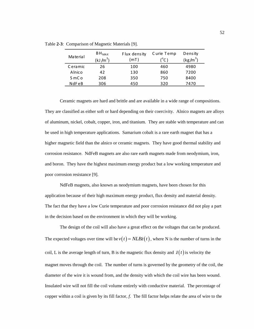
52
Ceramic magnets are hard and brittle and are available in a wide range of compositions.
They are classified as either soft or hard depending on their coercivity. Alnico magnets are alloys
of aluminum, nickel, cobalt, copper, iron, and titanium. They are stable with temperature and can
be used in high temperature applications. Samarium cobalt is a rare earth magnet that has a
higher magnetic field than the alnico or ceramic magnets. They have good thermal stability and
corrosion resistance. NdFeB magnets are also rare earth magnets made from neodymium, iron,
and boron. They have the highest maximum energy product but a low working temperature and
poor corrosion resistance [9].
NdFeB magnets, also known as neodymium magnets, have been chosen for this
application because of their high maximum energy product, flux density and material density.
The fact that they have a low Curie temperature and poor corrosion resistance did not play a part
in the decision based on the environment in which they will be working.
The design of the coil will also have a great effect on the voltages that can be produced.
The expected voltages over time will be v t NLBz t , where N is the number of turns in the
coil, L is the average length of turn, B is the magnetic flux density and z t is velocity the
magnet moves through the coil. The number of turns is governed by the geometry of the coil, the
diameter of the wire it is wound from, and the density with which the coil wire has been wound.
Insulated wire will not fill the coil volume entirely with conductive material. The percentage of
copper within a coil is given by its fill factor, f. The fill factor helps relate the area of wire to the
Table 2-3: Comparison of Magnetic Materials [9].
MaterialB HMAX
(kJ /m3)
F lux dens ity(mT )
C urie T emp
(oC )
Dens ity
(kg/m3)
C eramic 26 100 460 4980Alnico 42 130 860 7200S mC o 208 350 750 8400NdF eB 306 450 320 7470
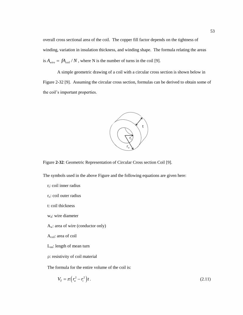
53
overall cross sectional area of the coil. The copper fill factor depends on the tightness of
winding, variation in insulation thickness, and winding shape. The formula relating the areas
is NfAA coilwire / , where N is the number of turns in the coil [9].
A simple geometric drawing of a coil with a circular cross section is shown below in
Figure 2-32 [9]. Assuming the circular cross section, formulas can be derived to obtain some of
the coil’s important properties.
The symbols used in the above Figure and the following equations are given here:
ri: coil inner radius
ro: coil outer radius
t: coil thickness
wd: wire diameter
Aw: area of wire (conductor only)
Acoil: area of coil
Lmt: length of mean turn
ρ: resistivity of coil material
The formula for the entire volume of the coil is:
2 2
T o iV r r t . (2.11)
Figure 2-32: Geometric Representation of Circular Cross section Coil [9].

54
The formula for length of wire needed to wind a coil for a specific volume is:
2
4 Tw
d
fVL
w . (2.12)
The coil resistance formula is then:
2
o iw mtc
w w o i
N r rL NLR
A A f r r t
. (2.13)
Finally, the number of turns in the coil can be found by the following formula:
2
w
o i
i
LN
r rr
. (2.14)
Using all of these formulas it is possible to determine the voltage that a coil and magnet
will produce based on the velocity of the proof mass, which in this case will be the magnet. As
already discussed , however, the voltage generated will differ from what is predicted by the
equation due to the differences in magnet and coil placement.
Chapter 2 has discussed the base motion and centrifugal forces an electromagnetic
harvester with a proof mass will experience. Different design ideas were discussed and analyzed
to see if they would be practical to implement and also if they could meet the power
requirements. The quality factor and frequency ratio of each design has led to the further
development of the reverse centrifugal pendulum design, which analytically performed well in
both categories. The next chapter will discuss the implementation of the reverse centrifugal
pendulum harvester design and the experimental procedure used to test it.

Chapter 3
Experimental Testing of Energy Harvesting Device
This chapter details the fabrication of the harvesting device, the electronics associated
with it, and the experimental set up and procedure used to test the device. Predictions on mass
motion, voltage generated, and power generated are given and compared with their experimental
values. Two different harvesters are built, however only one is tested due to time constraints.
The goal of the chapter is to build an energy harvester based on the reverse pendulum design and
to experimentally evaluate the device and compare the results to analytical predictions.
3.1 Experimental Procedure
The experimental procedure used to test the device is designed to gain a full
understanding of the dynamics of each system and obtain estimates of system properties. A base
motion system was constructed to match the frequency and amplitude of the pitch link for
different pilot inputs. This enabled the harvester to be subjected to the whole range of flight
conditions it would see in flight. The centrifugal force was simulated with a mass and pulley
system that will be described later. For operational procedures of the base motion system, refer to
Appendix A.
First, system parameters k, m, and ζm were experimentally measured. These values were
used to update the analytical model to predict mass motion and voltage. The mass motion was
then obtained experimentally at all flight conditions from 1o cyclic to 15
o cyclic. The coil then
allowed AC voltages to be measured. At this point it can be determined if the voltage needs to be
stepped up and if there is a way to accomplish that. Finally, a representative load is placed to

56
draw current and measure the power output of the device. This procedure is outlined in the
following flowchart.
At all stages of experimentation, results are compared to predictions made using the
analytical model in MATLAB and Simulink. The experiment is first done without any
centrifugal force to obtain baseline parameters. Increasing increments of force are then placed on
the device to study trends and verify predictions. The next section describes the setup built to
carry out the experiment.
Figure 3-1: Flowchart of Experimental Procedure for Testing of Harvester. This is the procedure
that should be used to obtain useful power.
Obtain system parameters
experimentally (k, m, ζm)
Measure mass motion
at all flight conditions
Update analytical
model
Predict motion
and compare to
experiment
Add coil and
obtain AC
voltages
Step up
voltage?
Place simulated
load and obtain
power
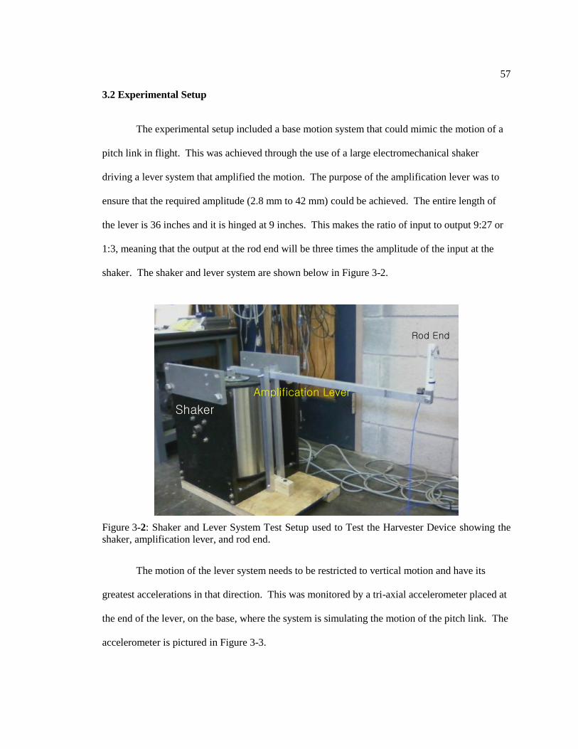
57
3.2 Experimental Setup
The experimental setup included a base motion system that could mimic the motion of a
pitch link in flight. This was achieved through the use of a large electromechanical shaker
driving a lever system that amplified the motion. The purpose of the amplification lever was to
ensure that the required amplitude (2.8 mm to 42 mm) could be achieved. The entire length of
the lever is 36 inches and it is hinged at 9 inches. This makes the ratio of input to output 9:27 or
1:3, meaning that the output at the rod end will be three times the amplitude of the input at the
shaker. The shaker and lever system are shown below in Figure 3-2.
The motion of the lever system needs to be restricted to vertical motion and have its
greatest accelerations in that direction. This was monitored by a tri-axial accelerometer placed at
the end of the lever, on the base, where the system is simulating the motion of the pitch link. The
accelerometer is pictured in Figure 3-3.
Figure 3-2: Shaker and Lever System Test Setup used to Test the Harvester Device showing the
shaker, amplification lever, and rod end.
Shaker
Amplification Lever
Rod End
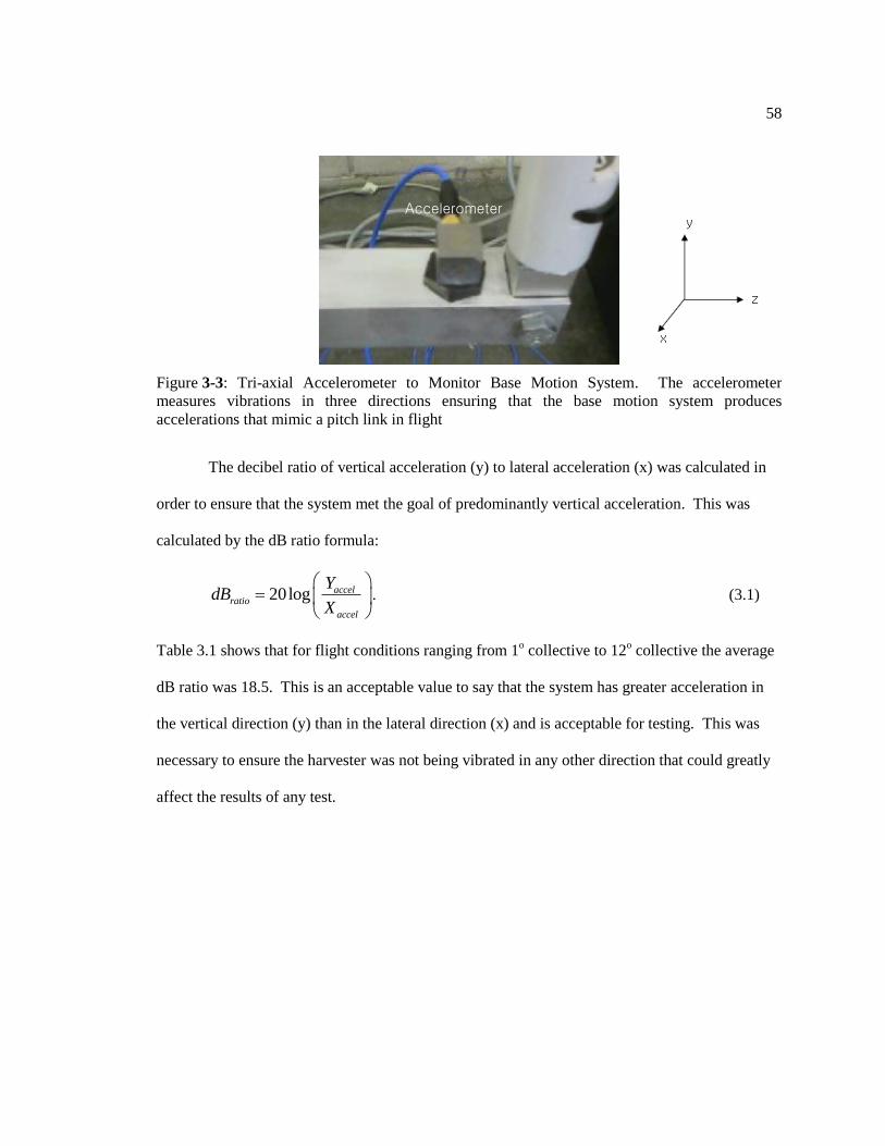
58
The decibel ratio of vertical acceleration (y) to lateral acceleration (x) was calculated in
order to ensure that the system met the goal of predominantly vertical acceleration. This was
calculated by the dB ratio formula:
20log accelratio
accel
YdB
X
. (3.1)
Table 3.1 shows that for flight conditions ranging from 1o collective to 12
o collective the average
dB ratio was 18.5. This is an acceptable value to say that the system has greater acceleration in
the vertical direction (y) than in the lateral direction (x) and is acceptable for testing. This was
necessary to ensure the harvester was not being vibrated in any other direction that could greatly
affect the results of any test.
Figure 3-3: Tri-axial Accelerometer to Monitor Base Motion System. The accelerometer
measures vibrations in three directions ensuring that the base motion system produces
accelerations that mimic a pitch link in flight
Accelerometer

59
The shaker is driven by an amplifier that is controlled by a signal generator. The output
of the signal generator and the output of the tri-axial accelerometer were monitored by an
oscilloscope to ensure that the correct inputs to the shaker were being made for the different flight
conditions. Figure 3-4 below gives an example oscilloscope reading. The top (yellow) line
indicates the output from the amplifier driving the shaker and the bottom (blue) line indicates the
output from the accelerometer at the base of the system.
Table 3-1: Vertical to Lateral Acceleration dB Ratios.
Acceleration (m/s2) Accel Decibel Ratio
2.04 19.534.09 16.276.13 19.018.25 21.3510.29 22.3512.34 17.9114.38 18.0216.43 17.2418.54 16.5820.59 17.4922.63 17.3824.68 15.63
Figure 3-4: Oscilloscope Output Monitoring Base Motion System. The top waveform
indicates the signal being sent to amplifier and the bottom wave indicates the signal from the
accelerometer monitoring the base motion system
Signal from Amp
Signal from
Accelerometer

60
An overall schematic of the test rig is in Figure 3-5. This drawing shows the shaker, amplifier
level, rod end, tri-axial accelerometer for monitoring the base motion, the signal generator and
amplifier that drive the shaker, and the oscilloscope that monitors the system
Both harvesters were designed to operate under high centrifugal forces. In order to
simulate this force a mass and pulley system was constructed. The goal of the mass-pulley
system is to put a constant force on the proof mass equal to the centrifugal force it would see in
the pitch link under rotation. A schematic and picture of the system is shown below in Figure 3-
6.
Figure 3-5: Overall Test Stand Schematic. The test rig includes the signal generator, amplifier,
shaker, and amplification lever as the base motion system and the accelerometer and oscilloscope
used to monitor it.
Figure 3-6: Mass-Pulley System to Simulate the Centrifugal Force.
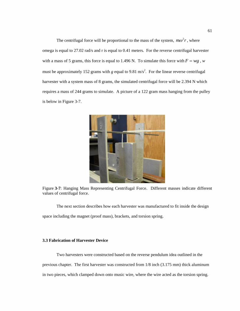
61
The centrifugal force will be proportional to the mass of the system, 2m r , where
omega is equal to 27.02 rad/s and r is equal to 0.41 meters. For the reverse centrifugal harvester
with a mass of 5 grams, this force is equal to 1.496 N. To simulate this force with F wg , w
must be approximately 152 grams with g equal to 9.81 m/s2. For the linear reverse centrifugal
harvester with a system mass of 8 grams, the simulated centrifugal force will be 2.394 N which
requires a mass of 244 grams to simulate. A picture of a 122 gram mass hanging from the pulley
is below in Figure 3-7.
The next section describes how each harvester was manufactured to fit inside the design
space including the magnet (proof mass), brackets, and torsion spring.
3.3 Fabrication of Harvester Device
Two harvesters were constructed based on the reverse pendulum idea outlined in the
previous chapter. The first harvester was constructed from 1/8 inch (3.175 mm) thick aluminum
in two pieces, which clamped down onto music wire, where the wire acted as the torsion spring.
Figure 3-7: Hanging Mass Representing Centrifugal Force. Different masses indicate different
values of centrifugal force.

62
The wire was 0.012 inches (0.305 mm) in diameter and provided a torsion spring constant of
.0187 N-m. Clamping onto the wire proved to be a challenge and many different ways of
accomplishing it were evaluated. The final solution was to use a screw that tightened the two
halves together. A CAD drawing of the device can be seen in Figure 3-8. The screw is shown in
the photo of the device in Figure 3-9.
Figure 3-8: CAD Drawing of Reverse Pendulum Harvester. The harvester was cut from a water
jet machine in two pieces. The two aluminum pieces were clamped with a screw onto a magnet
and a piece of music wire that acted as a spring
Figure 3-9: Photo of the Reverse Pendulum Harvester showing how the device looks after
completion.

63
The magnet used in the device was a neodymium magnet with a flux density of 0.7172
Teslas and a mass of 3 grams. The total device volume and mass were 3.84 cm3 and 5 grams.
The maximum vertical mass motion of the center of gravity of this device is limited to 0.5 inches
(12.7 mm). This design does not allow the magnet to pass through the center of a cylindrical coil.
The coil was placed next to the moving magnet in the experiment. This arrangement still allowed
voltage to be generated. The difference in voltage generated for a magnet in the center of a coil
versus a magnet next to a coil will be discussed in Section 3.5.4.
The second device built was also based on the reverse pendulum design with the
exception that the magnet was restricted to mostly vertical motion. This allowed the coil to be
placed around the magnet, in theory generating more voltage than placing the coil near the
magnet. This device also had a torsion spring but included three hinges as seen in the CAD
drawing below.
Figure 3-10: CAD Drawing of Linear Reverse Pendulum Harvester. This device also utilized
music wire to act as a spring but required three hinges which increased mechanical damping.

64
The magnet used in the linear reverse pendulum harvester was also a neodymium magnet
with a flux density of 0.7172 Teslas and having a mass of 3.02 grams. The total device volume is
12.29 cm3 and has a total mass of 8 grams. This design allows a maximum mass motion of 0.5
inches (12.7 mm) vertically from its equilibrium position. A free body diagram of this device is
shown below. The following analysis shows that this configuration produces the same
differential equation of motion and therefore will dynamically act the same as the reverse
pendulum harvester.
Figure 3-11: Photo of Linear Reverse Pendulum Harvester. The magnet was attached with spring
pins. The top back hinge is a Teflon rod and the other two hinges are shoulder bolts. Plastic
spacers were used to keep the device in line

65
Summing the forces in the x direction, it can be seen that Fa + Fb = CF and that Fa = Fb
because of symmetry. Therefore Fa = 1/2*CF. This will be important when summing moments
about point b which contains the torsional spring. Table 3-2 below summarizes the forces acting
on the mass with the small angle assumption.
Figure 3-12: Linear Reverse Pendulum Harvester Free Body Diagram shows that it is the same
dynamic system as the Reverse Pendulum Harvester Design.
Table 3-2: Forces Acting on Proof Mass.
Force Arm
CF:
IF:
Fd:
SF:
2m r
mx m z y
/ 2z L
e r
e rDz
ZK K
e r
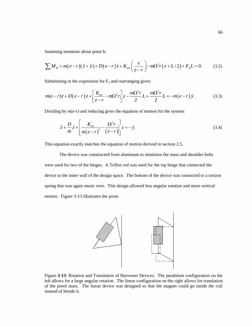
66
Summing moments about point b:
2 / 2 0B tor A
zM m e r z y D e r z K m r z L F L
e r
. (3.2)
Substituting in the expression for Fa and rearranging gives:
2 2
2( )2 2
torK m r m rm e r z D e r z m r z L L m e r y
e r
. (3.3)
Dividing by m(e-r) and reducing gives the equation of motion for the system:
2
2
torKD rz z z y
m e rm e r
. (3.4)
This equation exactly matches the equation of motion derived in section 2.5.
The device was constructed from aluminum to minimize the mass and shoulder bolts
were used for two of the hinges. A Teflon rod was used for the top hinge that connected the
device to the inner wall of the design space. The bottom of the device was connected to a torsion
spring that was again music wire. This design allowed less angular rotation and more vertical
motion. Figure 3-13 illustrates the point.
Figure 3-13: Rotation and Translation of Harvester Devices. The pendulum configuration on the
left allows for a large angular rotation. The linear configuration on the right allows for translation
of the proof mass. The linear device was designed so that the magnet could go inside the coil
instead of beside it.
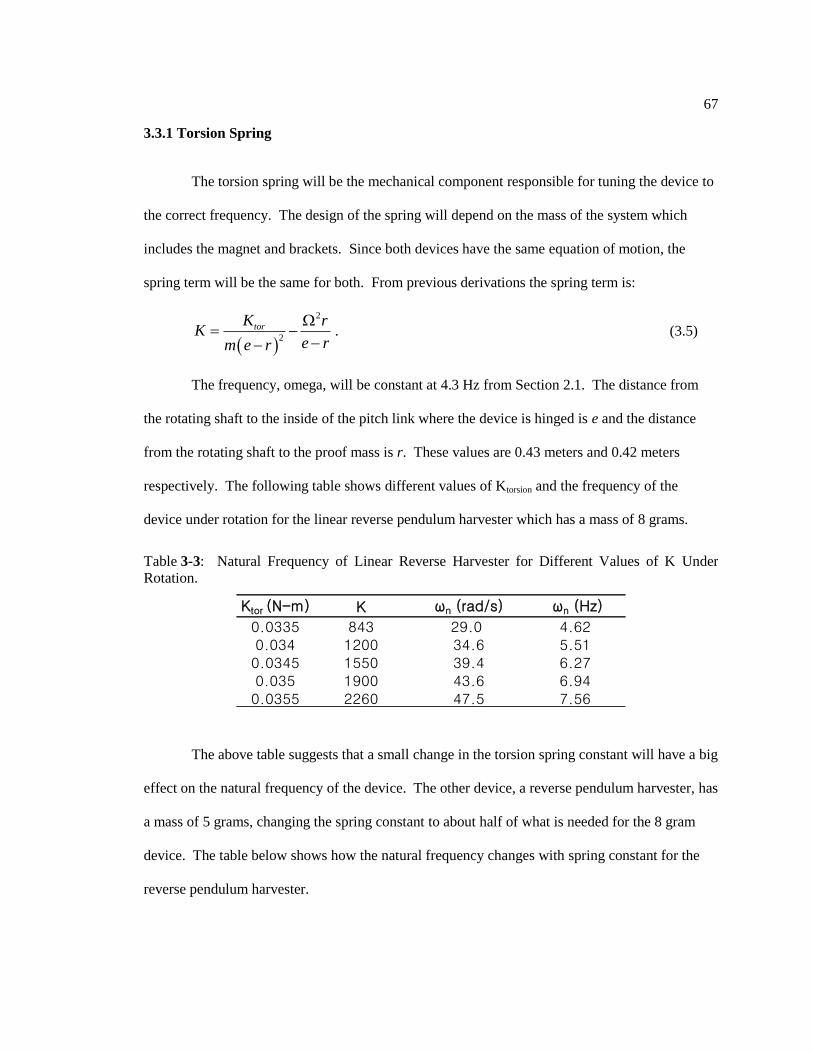
67
3.3.1 Torsion Spring
The torsion spring will be the mechanical component responsible for tuning the device to
the correct frequency. The design of the spring will depend on the mass of the system which
includes the magnet and brackets. Since both devices have the same equation of motion, the
spring term will be the same for both. From previous derivations the spring term is:
2
2
torK rK
e rm e r
. (3.5)
The frequency, omega, will be constant at 4.3 Hz from Section 2.1. The distance from
the rotating shaft to the inside of the pitch link where the device is hinged is e and the distance
from the rotating shaft to the proof mass is r. These values are 0.43 meters and 0.42 meters
respectively. The following table shows different values of Ktorsion and the frequency of the
device under rotation for the linear reverse pendulum harvester which has a mass of 8 grams.
The above table suggests that a small change in the torsion spring constant will have a big
effect on the natural frequency of the device. The other device, a reverse pendulum harvester, has
a mass of 5 grams, changing the spring constant to about half of what is needed for the 8 gram
device. The table below shows how the natural frequency changes with spring constant for the
reverse pendulum harvester.
Table 3-3: Natural Frequency of Linear Reverse Harvester for Different Values of K Under
Rotation.
Ktor (N-m) K ωn (rad/s) ωn (Hz)
0.0335 843 29.0 4.620.034 1200 34.6 5.510.0345 1550 39.4 6.270.035 1900 43.6 6.940.0355 2260 47.5 7.56
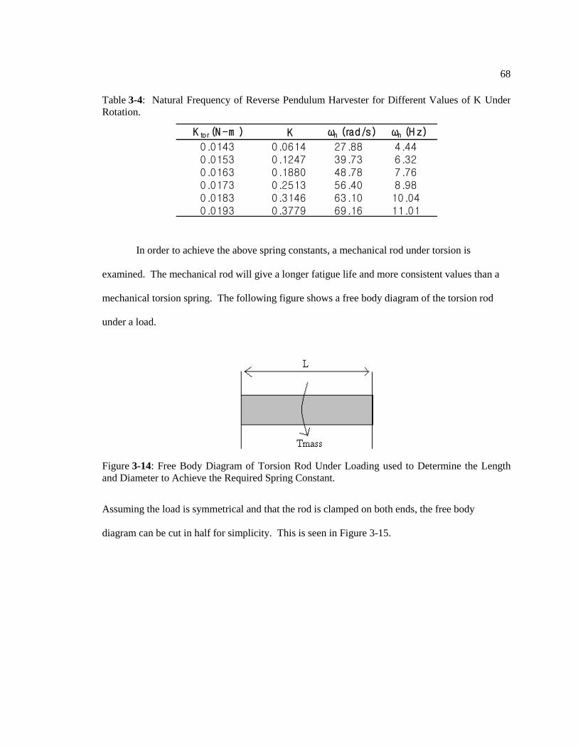
68
In order to achieve the above spring constants, a mechanical rod under torsion is
examined. The mechanical rod will give a longer fatigue life and more consistent values than a
mechanical torsion spring. The following figure shows a free body diagram of the torsion rod
under a load.
Assuming the load is symmetrical and that the rod is clamped on both ends, the free body
diagram can be cut in half for simplicity. This is seen in Figure 3-15.
Table 3-4: Natural Frequency of Reverse Pendulum Harvester for Different Values of K Under
Rotation.
K tor (N -m ) K ωn (rad/s) ωn (H z)
0.0143 0.0614 27.88 4.440.0153 0.1247 39.73 6.320.0163 0.1880 48.78 7.760.0173 0.2513 56.40 8.980.0183 0.3146 63.10 10.040.0193 0.3779 69.16 11.01
Figure 3-14: Free Body Diagram of Torsion Rod Under Loading used to Determine the Length
and Diameter to Achieve the Required Spring Constant.
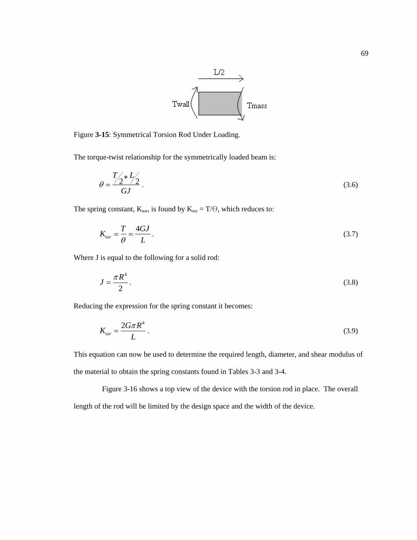
69
The torque-twist relationship for the symmetrically loaded beam is:
2 2T L
GJ
. (3.6)
The spring constant, Ktor, is found by Ktor = T/θ, which reduces to:
4
tor
T GJK
L . (3.7)
Where J is equal to the following for a solid rod:
4
2
RJ
. (3.8)
Reducing the expression for the spring constant it becomes:
42tor
G RK
L
. (3.9)
This equation can now be used to determine the required length, diameter, and shear modulus of
the material to obtain the spring constants found in Tables 3-3 and 3-4.
Figure 3-16 shows a top view of the device with the torsion rod in place. The overall
length of the rod will be limited by the design space and the width of the device.
Figure 3-15: Symmetrical Torsion Rod Under Loading.

70
Due to the aforementioned constraints, the maximum length of the rod was found to be
0.4 inches (10.16 mm). Initially, different polymers were researched with standard stock
diameters of 1/16 inch (1.59 mm) to 1/4 inch (6.35 mm). Given the shear moduli of the polymers
like PEEK©, the required length of the rod to achieve the necessary spring constant is greater
than the maximum of 0.4 inches (10.16 mm) allowed by the design constraints. The only other
property of the rod that could be changed was the diameter. Steel music spring wire has a shear
modulus of 80 GPa which is much greater than that of plastics, but it can be manufactured with
diameters as low as 0.004”. Using steel music wire with a shear modulus of 80 GPa and a length
of 0.4 inches (10.16 mm), the following table shows the required diameter to achieve the spring
constant desired. Table 3-5 is for the linear reverse pendulum harvester design with a mass of 8
grams and the second table is for the reverse pendulum harvester design with a mass of 5 grams.
Figure 3-16: Top View of Harvester Device with Torsion Rod shows how the length of the rod
will impact dimensions for the rest of the device.

71
Steel music wire with diameters of 0.012 inches (0.305 mm) and 0.015 inches (0.381
mm) were used. The spring constant will change based on the tolerance of the wire diameter, the
ability to clamp the length to 0.4 inches (10.16 mm) and the shear modulus of the steel. Based on
these variables, the natural frequency of the system will change. It was therefore necessary to
measure some of these properties and take into account the tolerance of the wire when predicting
what spring constant the wire will actually provide.
3.4 Device Circuitry
The final goal of powering a sensor has to be achieved with some circuitry that converts
the AC voltage into useful DC voltage. The first step is to take the AC voltage that is produced
Table 3-5: Required Diameter of Wire to achieve Spring Constant for Linear Device.
Ktor (N-m) Length (m) Radius (m) Diameter (in)
0.0335 0.01016 0.0001918 0.01510.034 0.01016 0.0001925 0.01520.0345 0.01016 0.0001932 0.01520.035 0.01016 0.0001939 0.01530.0355 0.01016 0.0001946 0.01530.036 0.01016 0.0001953 0.01540.0365 0.01016 0.000196 0.0154
Table 3-6: Required Diameter of Wire to achieve Spring Constant for Reverse Pendulum.
Ktor (N-m) Length (m) Radius (m) Diameter (in)
0.0167 0.01016 0.0001612 0.01270.0168 0.01016 0.0001614 0.01270.0169 0.01016 0.0001617 0.01270.017 0.01016 0.0001619 0.01270.0171 0.01016 0.0001621 0.01280.0172 0.01016 0.0001624 0.01280.0173 0.01016 0.0001626 0.0128

72
by the harvester and pass it through a bridge rectifier that converts it to DC voltage. A bridge
rectifier is made from four diodes that only allow the positive current to flow one direction and
the negative current to flow in the other direction, thus producing direct current. A schematic of a
full bridge rectifier is shown below.
To illustrate the circuit design process a model was created in Simulink and MATLAB.
The model included an AC voltage source that represented the energy harvester and was set to 1
volt. One volt was chosen after some preliminary experiments. This was connected to a step up
transformer and then into the bridge rectifier to produce the necessary DC voltage. The circuit
was completed with a resistive load. The schematic below shows the entire circuit.
Figure 3-17: Bridge Rectifier Schematic. Four diodes can be used to construct a bridge rectifier
that converts AC voltage to DC voltage.
Figure 3-18: Circuit Schematic used for Design. Circuit needed to produce useful DC voltages
from the AC voltages produced by the harvester
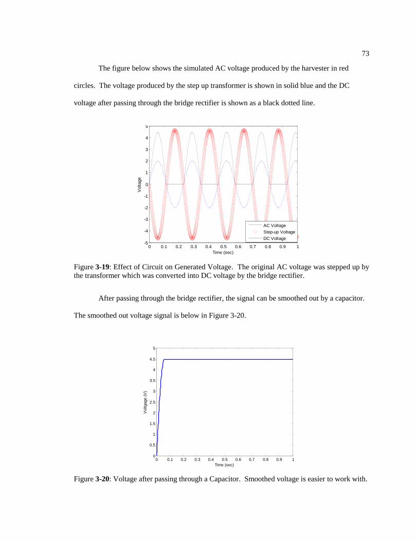
73
The figure below shows the simulated AC voltage produced by the harvester in red
circles. The voltage produced by the step up transformer is shown in solid blue and the DC
voltage after passing through the bridge rectifier is shown as a black dotted line.
After passing through the bridge rectifier, the signal can be smoothed out by a capacitor.
The smoothed out voltage signal is below in Figure 3-20.
0 0.1 0.2 0.3 0.4 0.5 0.6 0.7 0.8 0.9 1-5
-4
-3
-2
-1
0
1
2
3
4
5
Time (sec)
Voltage
Time v Voltage
AC Voltage
Step-up Voltage
DC Voltage
Figure 3-19: Effect of Circuit on Generated Voltage. The original AC voltage was stepped up by
the transformer which was converted into DC voltage by the bridge rectifier.
0 0.1 0.2 0.3 0.4 0.5 0.6 0.7 0.8 0.9 10
0.5
1
1.5
2
2.5
3
3.5
4
4.5
5
Time (sec)
Voltgage (
V)
Figure 3-20: Voltage after passing through a Capacitor. Smoothed voltage is easier to work with.

74
This voltage can now be used to power any sensor or a voltage regulator can be used to
keep the voltage supply steady. The final design of the circuit may not include a transformer but
may include a DC to DC converter that helps to step up the voltage. It will depend on the
voltages produced by the harvester as to whether or not a voltage boost is needed. Silicon diodes
have a voltage drop of 700 mV across them. If the voltage produced by the harvester is too low,
then a bridge rectifier will kill the signal. In this case, a transformer could be used to boost the
voltage before it is rectified. If the voltage produced by the harvester is an acceptable level (large
enough not to kill the signal with a 1.4 volt drop), than the DC-DC converter can be used.
3.5 Testing of Device
Two different mechanical devices based on the reverse pendulum design were built but
only one was tested. The mechanical differences have already been discussed. In this section the
first reverse pendulum device will be tested to see if predictions made during the design process
can be validated. First, the natural frequency of the device will be tested with and without the
effect of the centrifugal force. Then the mechanical damping of the device will be measured to
estimate system losses. Finally, predictions on mass motion, voltage generated and power
generated will be tested for validation.
3.5.1 Natural Frequency Prediction and Validation
The reverse pendulum device was built to operate at approximately 1/rev which is about
4.3 Hz. This was achieved through the use of a thin music wire as the torsion spring with a
diameter of 0.012 inches (0.305 mm). In order to obtain the natural frequency of the device, a
laser vibrometer was used to measure the decay from an initial displacement test. Then, when the
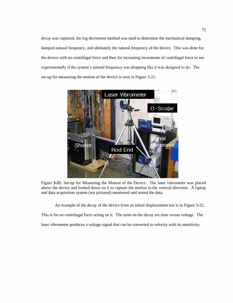
75
decay was captured, the log decrement method was used to determine the mechanical damping,
damped natural frequency, and ultimately the natural frequency of the device. This was done for
the device with no centrifugal force and then for increasing increments of centrifugal force to see
experimentally if the system’s natural frequency was dropping like it was designed to do. The
set-up for measuring the motion of the device is seen in Figure 3-21.
An example of the decay of the device from an initial displacement test is in Figure 3-22.
This is for no centrifugal force acting on it. The units on the decay are time versus voltage. The
laser vibrometer produces a voltage signal that can be converted to velocity with its sensitivity.
Figure 3-21: Set-up for Measuring the Motion of the Device. The laser vibrometer was placed
above the device and looked down on it to capture the motion in the vertical direction. A laptop
and data acquisition system (not pictured) monitored and stored the data.

76
From the above data it is possible to determine the damped natural frequency, the
mechanical damping, and the natural frequency of the device using the log decrement method.
The log decrement method says that the logarithmic decrement of the amplitudes of any two
successive peaks is:
01ln
n
x
n x
. (3.10)
Where x0 is the greater of the two amplitudes and xn is the amplitude of a peak n periods away.
Using the logarithmic decrement the damping ratio can be found by:
2
1
21
. (3.11)
The damped natural frequency is then found by the following equation, where T, the period of the
waveform, is the time between two successive peaks.
2
dT
. (3.12)
Finally, the undamped natural frequency of the device can be found:
Initial D isplacment Test
-8
-6
-4
-2
0
2
4
6
8
0 0.5 1 1.5 2
Time (s ec )
Vo
lta
ge
(V
)
Figure 3-22: Exponential Decay from Initial Displacement Test. This is one example that was
used to calculate mechanical damping and natural frequency.

77
21
dn
. (3.13)
The above was done for the reverse pendulum harvester at increasing amounts of
centrifugal force and compared to predictions made about what should happen. The predictions
included physical measurements of the device, including the clamped length L of the music wire
from Section 3.3.1, the mass of the device, and the diameter of the wire. The wire diameter was
0.012 inches (0.305 mm) with a tolerance of 0.0003 inches (0.0076 mm). Shown below is a plot
of natural frequency vs. centrifugal force for both the experiment and what was predicted to
happen.
The natural frequency of the device found experimentally closely matched the model for
4 out of 5 data points up to 0.8 N of force, which is 68% of the full CF. The equation for natural
frequency as a function of centrifugal force can be found in the spring term of Equation 2.8. The
0
5
10
15
20
25
0 0.2 0.4 0.6 0.8 1 1.2 1.4
CF (N)
Natu
ral Fre
quency
(Hz)
Experiment
Predicted
Figure 3-23: Natural Frequency vs. Centrifugal Force. The predicted natural frequency of the
device matched the experiment for four out of five points and the data shows that increasing the
centrifugal force lowered the natural frequency of the harvester.

78
natural frequency will be the square root of that spring term because mass has already been
divided through the equation. The differences arose due to difficulties in accurately placing the
centrifugal force onto the mass of the harvester as seen in Figure 3-24. The two lines indicate the
direction of the centrifugal force. Whenever the force was not ideally placed on the mass, the
harvester did not respond like was predicted. When great care was taken to make the force act
linearly on the proof mass, the harvester responded as predicted. In order for the data to be
completely accurate a better method of simulating the centrifugal force would be needed.
However, the above data does prove the trend that the natural frequency is dropping with
increasing centrifugal force.
3.5.2 Mechanical and Electrical Damping
The initial displacement test and log decrement method described above can be used to
find the mechanical damping of the device. Because there is no coil on the device during these
Figure 3-24: Simulated Centrifugal Force on Proof Mass. Difficulties in pointing the CF linearly
on the proof mass contributed to the differences in experimental natural frequency vs. predicted.

79
tests, all of the damping will be mechanical. Once the coil is placed into the device, there will be
additional damping due to the magnet and coil interaction that will be part of the electrical
damping of the device and is essential to producing voltage and ultimately power. Table 3-7
shows the results for mechanical damping values at different centrifugal forces.
As expected, the mechanical damping ratio increases with increasing centrifugal force
due to increased material losses in the spring and the clamped ends of the spring. These values
represent pure mechanical loss in the system and ideally would be minimized in order to harvest
more power.
To find the electrical damping of the system, a resistor was placed across the ends of the
coil and the log decrement method was used to find total system damping. Then, knowing the
mechanical damping of the system, the remaining damping had to be electrical. From Equation
1.15, the electrical damping will be a function of resistance. Section 2.2.3 showed that the most
power is harvested when the electrical and mechanical dampings are matched. Figure 3-25 shows
the results of the experiment for five different resistor values. The dot on the graph indicates the
mechanical damping value of 0.0134. The 1000 ohm resistor provided the closest value to match
electrical damping to mechanical. For simplicity and accuracy, this was only done for the
harvester with no centrifugal force.
Table 3-7: Mechanical Damping Values.
CF (N) ωn ζ
0 18.46 0.0130.24 16.87 0.0140.47 16.31 0.0220.82 13.35 0.0241.18 11.82 0.036

80
To find the value of resistor that matches the electrical damping to mechanical without
having to experimentally determine it, Equation 1.15 can be utilized. Solving for R:
2
2 n
NLBR
m (3.14)
Where ζ will be the mechanical damping value that is trying to be matched, ωn is the
natural frequency of the device, m is the mass of the system, and N, L, and B are properties of the
coil and magnet. Table 3-8 gives the value of resistors that match electrical damping to
mechanical at different values of centrifugal force. This is necessary because mechanical
damping is a function of centrifugal force.
Electrical Damping vs Load Resistance
0
0.002
0.004
0.006
0.008
0.01
0.012
0.014
0.016
0 500 1000 1500 2000
Resistance (ohms)
Ele
ctric
al D
am
pin
g R
atio
Figure 3-25: Electrical Damping vs. Load Resistance. A resistor value of 1000 ohms closely
matches electrical to mechanical damping which is ideal for energy harvesting. The dot on the
graph indicates the mechanical damping value of 0.0134.
Table 3-8: Load Resistance as a Function of Centrifugal Force.
CF ζe R (Ω)
0 0.013 1171
0.24 0.015 1060
0.47 0.022 700
0.82 0.024 646
1.18 0.036 433

81
The calculated value of R that would match electrical to mechanical damping was found
to be 1170 ohms as compared to 1000 ohms experimentally.
3.5.3 Mass Motion Prediction and Validation
The mechanical damping and natural frequencies from Table 3-7 can now be used with
the analytical model developed in Matlab and Simulink to predict the response of the device to
different inputs. The laser vibrometer was once again used to measure the velocity of the device
at the different flight conditions described in Section 2.1. The base motion system described in
Section 3.2 was used to test the response at different flight conditions. This was first done for no
centrifugal force and then for increasing amounts of centrifugal force as was previously done.
The absolute velocity of the device was captured but it is the relative velocity of the proof mass
with respect to the base motion that is necessary to generate power. This was found by
subtracting the base velocity from the absolute velocity of the proof mass. Figure 3-26 is the
absolute measured velocity of the device from 1o cyclic to 10
o cyclic inputs versus the predicted
velocity from the model. Very good agreement is seen showing that the model can indeed predict
the response of the device.
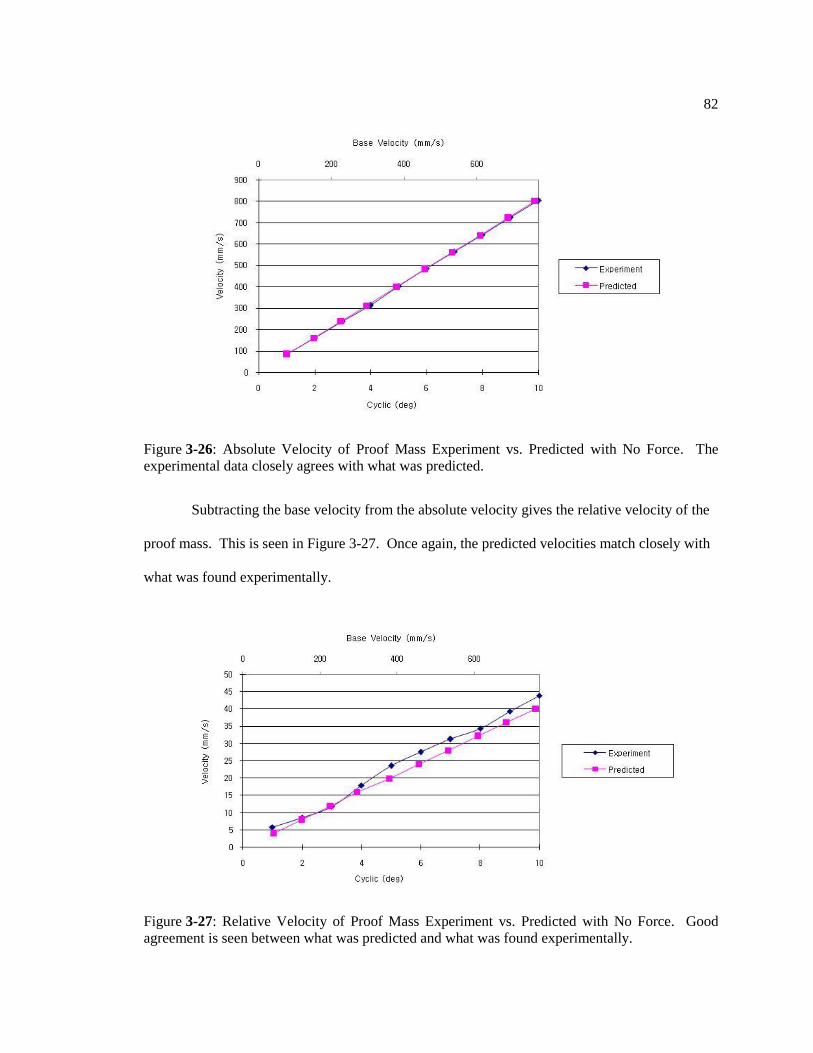
82
Subtracting the base velocity from the absolute velocity gives the relative velocity of the
proof mass. This is seen in Figure 3-27. Once again, the predicted velocities match closely with
what was found experimentally.
Figure 3-26: Absolute Velocity of Proof Mass Experiment vs. Predicted with No Force. The
experimental data closely agrees with what was predicted.
Figure 3-27: Relative Velocity of Proof Mass Experiment vs. Predicted with No Force. Good
agreement is seen between what was predicted and what was found experimentally.

83
Using these relative velocities, the voltage generated can be predicted. This will be done
in the next section. The absolute and relative velocities were also found with centrifugal force
being applied to the device. It was found earlier that the natural frequency dropped with applied
force but differences arose due to difficulties in correctly applying the force. Therefore, we
would expect that differences would arise in velocity prediction versus what was observed
experimentally. Figure 3-27 shows the absolute velocity versus what was predicted for 0.47 N of
centrifugal force. Experimentally the natural frequency with this force was found to be 16.3 Hz
while the prediction was 15.12 Hz. There appears to be good agreement with this data.
Figure 3-29 is the relative velocity of the proof mass with respect to the base motion.
The differences in predicted versus experiment are more apparent here and are expected due to
the differences in natural frequency.
Figure 3-28: Absolute Velocity of Proof Mass Experiment vs. Predicted for 0.47 N of Force.
This data also shows good agreement between prediction and experiment
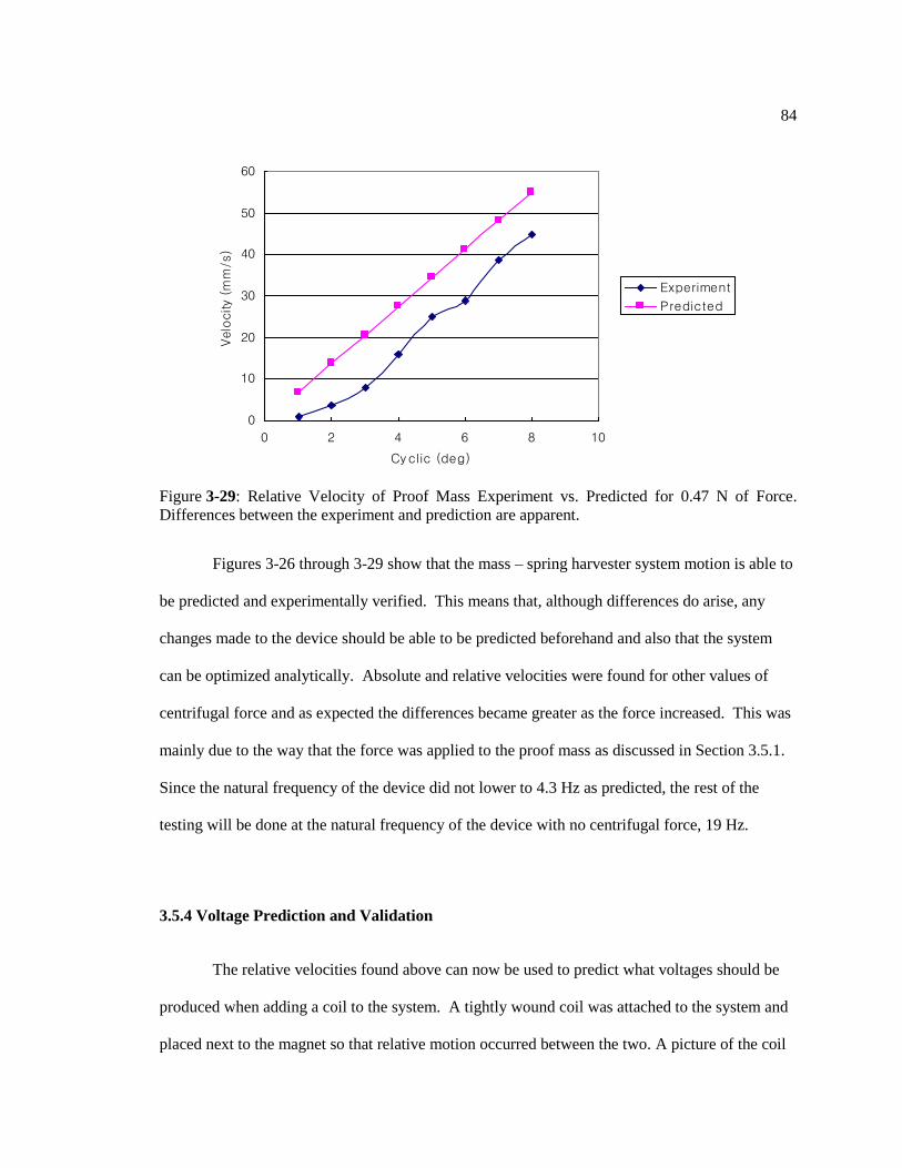
84
Figures 3-26 through 3-29 show that the mass – spring harvester system motion is able to
be predicted and experimentally verified. This means that, although differences do arise, any
changes made to the device should be able to be predicted beforehand and also that the system
can be optimized analytically. Absolute and relative velocities were found for other values of
centrifugal force and as expected the differences became greater as the force increased. This was
mainly due to the way that the force was applied to the proof mass as discussed in Section 3.5.1.
Since the natural frequency of the device did not lower to 4.3 Hz as predicted, the rest of the
testing will be done at the natural frequency of the device with no centrifugal force, 19 Hz.
3.5.4 Voltage Prediction and Validation
The relative velocities found above can now be used to predict what voltages should be
produced when adding a coil to the system. A tightly wound coil was attached to the system and
placed next to the magnet so that relative motion occurred between the two. A picture of the coil
Relative velocity Experiment vs Predicted
0
10
20
30
40
50
60
0 2 4 6 8 10
Cyclic (deg)
Velo
city
(mm
/s)
Experiment
Predicted
Figure 3-29: Relative Velocity of Proof Mass Experiment vs. Predicted for 0.47 N of Force.
Differences between the experiment and prediction are apparent.
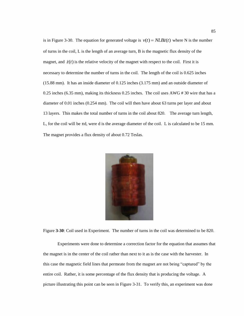
85
is in Figure 3-30. The equation for generated voltage is ( ) ( )v t NLBz t where N is the number
of turns in the coil, L is the length of an average turn, B is the magnetic flux density of the
magnet, and ( )z t is the relative velocity of the magnet with respect to the coil. First it is
necessary to determine the number of turns in the coil. The length of the coil is 0.625 inches
(15.88 mm). It has an inside diameter of 0.125 inches (3.175 mm) and an outside diameter of
0.25 inches (6.35 mm), making its thickness 0.25 inches. The coil uses AWG # 30 wire that has a
diameter of 0.01 inches (0.254 mm). The coil will then have about 63 turns per layer and about
13 layers. This makes the total number of turns in the coil about 820. The average turn length,
L, for the coil will be πd, were d is the average diameter of the coil. L is calculated to be 15 mm.
The magnet provides a flux density of about 0.72 Teslas.
Experiments were done to determine a correction factor for the equation that assumes that
the magnet is in the center of the coil rather than next to it as is the case with the harvester. In
this case the magnetic field lines that permeate from the magnet are not being “captured” by the
entire coil. Rather, it is some percentage of the flux density that is producing the voltage. A
picture illustrating this point can be seen in Figure 3-31. To verify this, an experiment was done
Figure 3-30: Coil used in Experiment. The number of turns in the coil was determined to be 820.
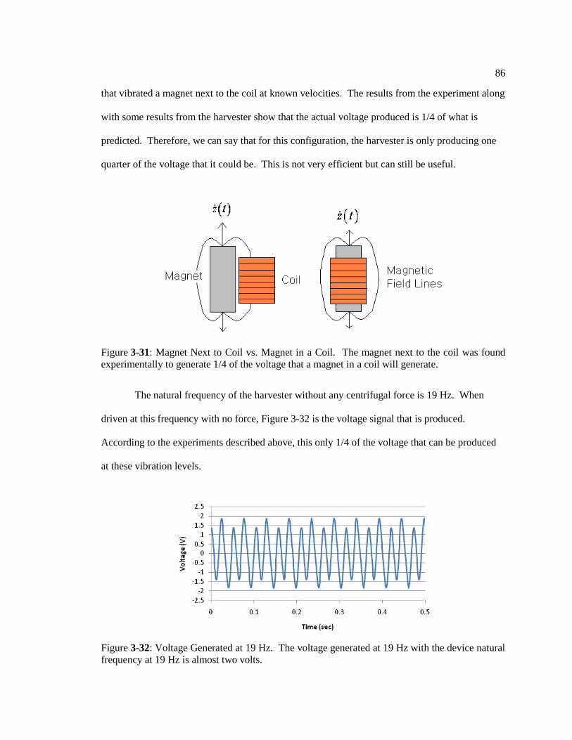
86
that vibrated a magnet next to the coil at known velocities. The results from the experiment along
with some results from the harvester show that the actual voltage produced is 1/4 of what is
predicted. Therefore, we can say that for this configuration, the harvester is only producing one
quarter of the voltage that it could be. This is not very efficient but can still be useful.
The natural frequency of the harvester without any centrifugal force is 19 Hz. When
driven at this frequency with no force, Figure 3-32 is the voltage signal that is produced.
According to the experiments described above, this only 1/4 of the voltage that can be produced
at these vibration levels.
Figure 3-31: Magnet Next to Coil vs. Magnet in a Coil. The magnet next to the coil was found
experimentally to generate 1/4 of the voltage that a magnet in a coil will generate.
Figure 3-32: Voltage Generated at 19 Hz. The voltage generated at 19 Hz with the device natural
frequency at 19 Hz is almost two volts.

87
The peak AC voltage produced at 19 Hz is almost 2 volts. Going back to the predictions
made about the voltage that would be produced, Figure 3-33 shows the voltage generated versus
the predicted voltage with no centrifugal force driven at 4.3 Hz. The predictions here include the
1/4 correction factor that was found. The results from the experiment now match up with the
prediction.
Figure 3-34 below shows the voltage generated versus frequency ratio for the harvester
with no force and the frequency ratio ranging from 0.89 to 1.1. As expected, the peak voltage
generated occurs when the driving frequency matches the natural frequency of the device.
Figure 3-33: Voltage Generated at 4.3 Hz with no Centrifugal Force. The empirically corrected
prediction compares favorably with the experimental data.
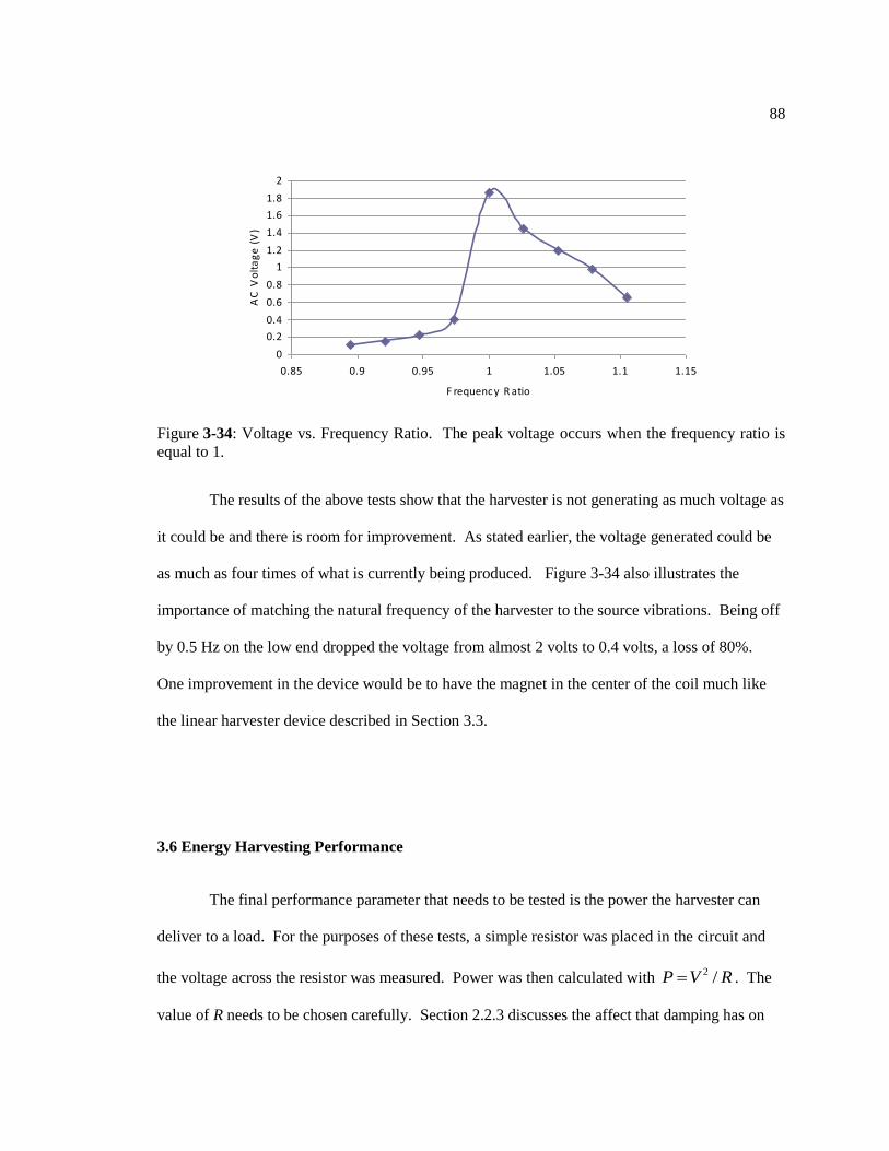
88
The results of the above tests show that the harvester is not generating as much voltage as
it could be and there is room for improvement. As stated earlier, the voltage generated could be
as much as four times of what is currently being produced. Figure 3-34 also illustrates the
importance of matching the natural frequency of the harvester to the source vibrations. Being off
by 0.5 Hz on the low end dropped the voltage from almost 2 volts to 0.4 volts, a loss of 80%.
One improvement in the device would be to have the magnet in the center of the coil much like
the linear harvester device described in Section 3.3.
3.6 Energy Harvesting Performance
The final performance parameter that needs to be tested is the power the harvester can
deliver to a load. For the purposes of these tests, a simple resistor was placed in the circuit and
the voltage across the resistor was measured. Power was then calculated with 2 /P V R . The
value of R needs to be chosen carefully. Section 2.2.3 discusses the affect that damping has on
0
0.2
0.4
0.6
0.8
1
1.2
1.4
1.6
1.8
2
0.85 0.9 0.95 1 1.05 1.1 1.15
F requency R atio
AC
Vo
lta
ge
(V
)
Figure 3-34: Voltage vs. Frequency Ratio. The peak voltage occurs when the frequency ratio is
equal to 1.
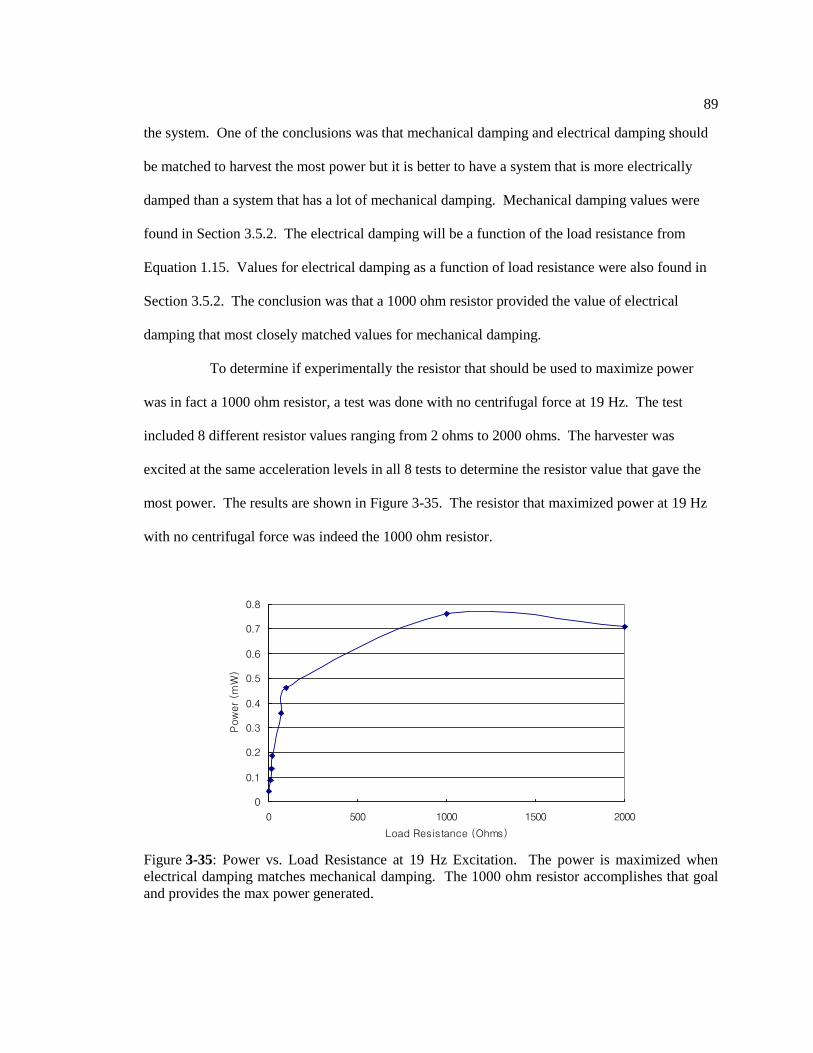
89
the system. One of the conclusions was that mechanical damping and electrical damping should
be matched to harvest the most power but it is better to have a system that is more electrically
damped than a system that has a lot of mechanical damping. Mechanical damping values were
found in Section 3.5.2. The electrical damping will be a function of the load resistance from
Equation 1.15. Values for electrical damping as a function of load resistance were also found in
Section 3.5.2. The conclusion was that a 1000 ohm resistor provided the value of electrical
damping that most closely matched values for mechanical damping.
To determine if experimentally the resistor that should be used to maximize power
was in fact a 1000 ohm resistor, a test was done with no centrifugal force at 19 Hz. The test
included 8 different resistor values ranging from 2 ohms to 2000 ohms. The harvester was
excited at the same acceleration levels in all 8 tests to determine the resistor value that gave the
most power. The results are shown in Figure 3-35. The resistor that maximized power at 19 Hz
with no centrifugal force was indeed the 1000 ohm resistor.
Power vs. Load Resistance
0
0.1
0.2
0.3
0.4
0.5
0.6
0.7
0.8
0 500 1000 1500 2000
Load Resistance (Ohms)
Pow
er (m
W)
Figure 3-35: Power vs. Load Resistance at 19 Hz Excitation. The power is maximized when
electrical damping matches mechanical damping. The 1000 ohm resistor accomplishes that goal
and provides the max power generated.
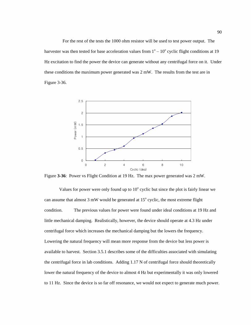
90
For the rest of the tests the 1000 ohm resistor will be used to test power output. The
harvester was then tested for base acceleration values from 1o – 10
o cyclic flight conditions at 19
Hz excitation to find the power the device can generate without any centrifugal force on it. Under
these conditions the maximum power generated was 2 mW. The results from the test are in
Figure 3-36.
Values for power were only found up to 10o cyclic but since the plot is fairly linear we
can assume that almost 3 mW would be generated at 15o cyclic, the most extreme flight
condition. The previous values for power were found under ideal conditions at 19 Hz and
little mechanical damping. Realistically, however, the device should operate at 4.3 Hz under
centrifugal force which increases the mechanical damping but the lowers the frequency.
Lowering the natural frequency will mean more response from the device but less power is
available to harvest. Section 3.5.1 describes some of the difficulties associated with simulating
the centrifugal force in lab conditions. Adding 1.17 N of centrifugal force should theoretically
lower the natural frequency of the device to almost 4 Hz but experimentally it was only lowered
to 11 Hz. Since the device is so far off resonance, we would not expect to generate much power.
Power vs Flight Condtion
0
0.5
1
1.5
2
2.5
0 2 4 6 8 10
Cyclic (deg)
Pow
er (m
W)
Figure 3-36: Power vs Flight Condition at 19 Hz. The max power generated was 2 mW.

91
Tests were done to determine exactly how much power could be generated, and the results were
on the order of microwatts. These results are not presented here.
Power to a load of 1000 ohms was achieved under ideal conditions at a higher frequency
than the frequency of the pitch link in flight. However, it does show that this configuration and
dimensions are capable of producing power on the order of milliwatts. If a more consistent way
to simulate centrifugal force could be achieved, then more power could be simulated at 4.3 Hz.
The main reason why power closer to milliwatts was not achieved at 4.3 Hz excitation was the
fact that the natural frequency of the device was almost three times that of the driving frequency.
Figure 2-12 shows how power drops off with frequency ratio. The frequency ratio here was
approximately 2.65, which is well off the best case scenario of a frequency ratio of 1 that was
achieved to produce Figure 3-36.

Chapter 4
Conclusion
The final chapter draws conclusions on the performance of the energy harvester and
makes recommendations on what aspects need to be improved and how the improvement can be
accomplished. One application of the energy harvester is to power a strain sensor and use the
data to predict retirement times. This application is detailed with some simulations using strain
data taken from a lead-lag damper in Appendix B. Finally, recommendations for future work on
the project are given.
4.1 Conclusions on Energy Harvester
The energy harvester developed and tested was based on pendulum configuration that
utilized a combination of a mechanical torsion spring made from music wire and the centrifugal
force from the rotation of the pitch link around the rotor as an effective spring constant. The
proof mass of the harvester was an NdFeB cylindrical magnet with a mass of 3.02 grams. The
coil used had 820 turns and was placed next to the vibrating magnet. The maximum power
generated at 19 Hz was 2 mW and was delivered to a load of 1 kilo-ohm. Simulations showed
that power ranging from a few milliwatts to 120 milliwatts were available to be harvested from
the environment. The 3 mW harvested indicates a very low efficiency of around 3% conversion.
The final energy harvester did not produce enough power at 4.3 Hz due to reasons
discussed in Section 3.6. However, there are many aspects of the design that can be improved.
The most obvious is developing a way to increase the voltage produced. One way this can be
done is through the use of a transformer with a turn ratio of at least 10:1. This would increase the

93
voltage ten times and allow it to be put through a bridge rectifier to produce DC voltage. One
problem that was already found with transformers is the frequency. Most commercial
transformers operate at 50 – 60 Hz or higher. No off-the-shelf transformers able to operate as low
as 4.3 Hz were found.
Another way of increasing the voltage that was already discussed is to design the
harvester in such a way that the magnet passes through the center of the coil instead of vibrating
beside it. One way this could be achieved is with the linear reverse pendulum harvester discussed
in Section 3.3 and shown in Figures 3-10 and 3-11. This device was built but not tested due to
time limitations. A device like this will have more mechanical damping because it requires three
hinges to operate but the voltage that can be generated may be as much as four times the amount
currently being generated. Another way to increase voltage is to use a coil with more turns. The
number of turns in the coil is directly proportional to the amount of voltage generated. A coil
with twice the number of turns would be able to produce twice the voltage, theoretically. The
limiting factor in sizing the coil, however, is the size of the hollow in the rod end. The coil that
was used was 0.25 inches (6.35 mm) in diameter and was close to being the biggest allowable
coil for the design space.
Voltage multiplier circuits were also looked at. Voltage multiplier circuits use diodes and
capacitors to either double, triple, or quadruple the voltage from an AC source to produce DC
voltage. A schematic of a voltage tripler circuit can be seen in Figure 4-1.

94
The drawback of voltage multiplier circuits is the voltage loss across the diodes. Silicon
diodes experience a voltage drop of 0.7 volts. Germanium diodes, which are more expensive and
harder to find, only have a voltage drop of 0.2 volts. Considering the low voltage already
produced by the harvester, large voltage drops are not ideal and should be minimized. Using a
voltage drop of 0.2 volts, some simulations were run with voltage doubler, tripler, and quadrupler
circuits. Figure 4-2 displays the results.
Figure 4-1: Voltage Tripler Circuit. A circuit like this would be able to triple the voltage
produced using diodes and capacitors.
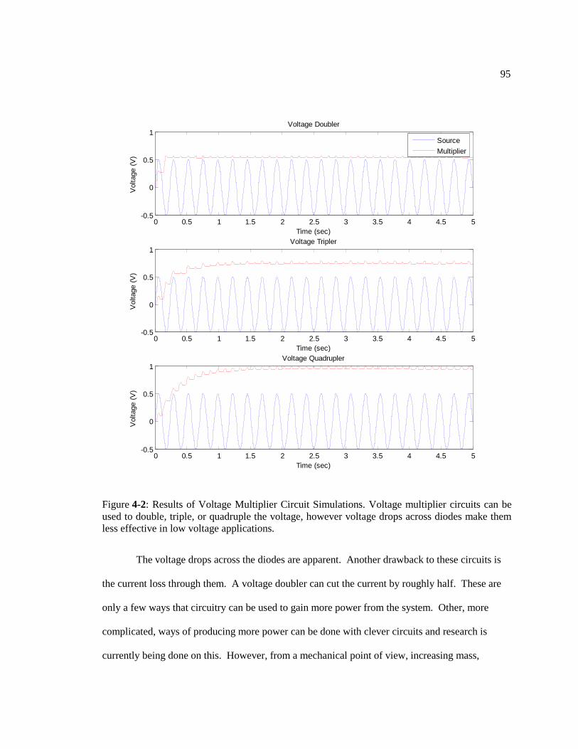
95
The voltage drops across the diodes are apparent. Another drawback to these circuits is
the current loss through them. A voltage doubler can cut the current by roughly half. These are
only a few ways that circuitry can be used to gain more power from the system. Other, more
complicated, ways of producing more power can be done with clever circuits and research is
currently being done on this. However, from a mechanical point of view, increasing mass,
0 0.5 1 1.5 2 2.5 3 3.5 4 4.5 5-0.5
0
0.5
1Voltage Quadrupler
Time (sec)
Voltage (
V)
0 0.5 1 1.5 2 2.5 3 3.5 4 4.5 5-0.5
0
0.5
1Voltage Doubler
Time (sec)
Voltage (
V)
0 0.5 1 1.5 2 2.5 3 3.5 4 4.5 5-0.5
0
0.5
1Voltage Tripler
Time (sec)
Voltage (
V)
Source
Multiplier
Figure 4-2: Results of Voltage Multiplier Circuit Simulations. Voltage multiplier circuits can be
used to double, triple, or quadruple the voltage, however voltage drops across diodes make them
less effective in low voltage applications.

96
quality factor, and coil size, or decreasing mechanical losses in the system are ways to generate
more power.
4.2 Future Work
Electromagnetic energy harvesting is not a new concept; however, applications to
rotorcraft and wireless sensors are still being explored. The next step in testing an
electromagnetic device would be to put it on a test stand that mimics the motion of a pitch link
but also spins, so that centrifugal force is created instead of simulated with a mass – pulley
system. If the device works under these conditions then the final step would be to implement any
circuit electronics and sensors. Ultimately, the final test would be a flight test, in which the
harvester powers a sensor, obtains data, and wirelessly transmits the data to a remote station.
Improvements for the energy harvester have been discussed in Section 4.1 and include
ways to boost the voltage through changes in the mechanical device and through added circuitry
and other electronic elements. Some of these changes should be implemented in order to improve
the power output of the device.
Only electromagnetic harvesting was thoroughly discussed here, however piezoelectric
harvesting should also be looked at. Piezoelectric devices are known to produce more voltage
then electromagnetic harvesters and have a greater power density, meaning more power can be
harvested from a smaller volume device. A piezoelectric device could be designed to work as a
resonant system similar to the electromagnetic device, or strains in rotorcraft components could
be used to produce power. This is similar to the MicroStrain© pitch link energy harvesting
system discussed in Section 1.3 [20].
97
References
[1] Lougee, Hoyt., 2002. “HUMS – Certification and Considerations for Current and
Emerging Technology,” IEEE 0-7803-7367-7
[2] Gill, John J., “Lessons Learned from Rotary and Fixed Wing HUMS
Applications,” BFGoodrich Aerospace, Bedford, Massachusetts
[3] Land, James E., 2001. “HUMS – The Benefits – Past, Present, and Future.” IEEE
0-7803-6599-2
[4] Sodano, H., Inman, D., “A Review of Power Harvesting from Vibration using
Piezoelectric Materials,” The Shock and Vibration Digest, 36(3), pp. 197-205, 2004
[5] Roundy, S., Wright, P., Rabaey, J., Energy Scavenging for Wireless Sensor
Networks with Special Focus on Vibrations, Kluwer Academic Publishers, 2004
[6] Mitcheson, P.D., Green, T.C., Yeatman, E.M. and Holmes, A.S. 2004.
“Architectures for Vibration-Driven Micropower Generators,” Journal of
Microelectromechanical Systems, 13(3):429 – 440
[7] Gilbert, James M., Balouchi, Farooq. 2008. “Comparison of Energy Harvesting
Systems for Wireless Sensor Networks,” International Journal of Automation and Computing,
5(4):334-347
[8] Thomson, W.T., Theory of Vibration with Applications, 2nd
Edition, Englewood
Cliffs, NJ: Prentice Hall, 1981
[9] Priya, S., Inman, D. (eds.), Energy Harvesting Technologies, Springer
Science+Business Media, LLC 2009
[10] Amirtharajah, Rajeevan, Chandrakasan, Anantha P., “Self Powered Signal
Processing Using Vibration Based Power Generation.” May 1998., IEEE Journal of Solid State
Circuits., vol. 33, No. 5.
[11] El-Hami, M., Glynne-Jones, P., White, N.M., Hill, M., Beeby, S., James, E.,
Brown, A.D., Ross, J.N., “Design and Fabrication of a New Vibration-based Electromechanical
Power Generator,” Sensors and Actuators, A 92, pp. 335-342, 2001
[12] Glynne- Jones, P., Tudor, M.J., Beeby, S.P., White, N.M., “An Electromagnetic,
Vibration-Powered Generator for Intelligent Sensor Systems,” Sensors and Actuators, A 110, pp.
344-349, 2004
[13] Beeby, S., Torah, R., Tudor, M., Glynne-Jones, P., O’Donnell, T., Saha, C., Roy,
S., “A Micro Electromagnetic Generator for Vibration Energy Harvesting,” Journal of
Micromechanics and Microengineering, 17: 1257-1265, 2007

98
[14] Beeby, S., Tudor, M., White, N., “Energy Harvesting Vibration Sources for
Microsystem Applications,” Measurement Science and Technology, 17: R175-R195, 2006
[15] Saha, C., O’Donnell, T., Loder, H., Beeby, S., and Tudor, J., “Optimization of an
Electromagnetic Energy Harvesting Device,” IEEE Transactions on Magnetics, vol. 42, no. 10,
October 2006
[16] Beeby, S., Tudor, M., Torah, R., Roberts, S., O’Donnell, T., Roy, S.,
“Experimental Comparison of Macro and Micro Scale Electromagnetic Vibration Powered
Generators,” Microsyst Technol, 13: 1647-1653, 2007
[17] Yuen, Steve C.L., Lee, Johnny M.H., Li, Wen J., Leung, Philip, H.W., “An AA-
Sized Vibration-Based Microgenerator for Wireless Sensors.” Pervasive Computing, January –
March 2007.
[18] Hadas, Z., Kluge, M., Singule, V., Ondrusek, C., “Electromagnetic Vibration
Power Generator,” IEEE International Symposium on Diagnostics for Electric Machines, Power
Electronics and Drives, SDEMPED, pp. 451-455, 2007.
[19] von Buren, T., Mitcheson, P., Green, T., Yeatman, E., Holmes, A., Troster, G.,
“Optimization of Inertial Micropower Generators for Human Walking Motion,” IEEE Sensors
Journal, vol. 6, no. 1, February 2006
[20] Arms, S., Townsend, C., Churchill, D., Augustin, M., Yeary, D., Darden, P.,
Phan, N., “Tracking Pitch Link Dynamic Loads with Energy Harvesting Wireless Sensors,”
Presented at the American Helicopter Society 63rd
Annual Forum, Virginia Beach, VA, May 1-3,
2007
[21] Arms, S., Townsend, C., Churchill, D., Moon, S., Phan, N., “Energy Harvesting
Wireless Sensors for Helicopter Damage Tracking,” Presented at the American Helicopter
Society 62nd
Annual Forum, Phoenix, AZ, May 9-11, 2006
[22] Churchill, D., Hamel, M., Townsend, C., Arms, S., “Strain Energy Harvesting for
Wireless Sensor Networks,” Smart Structures and Materials, Proceedings of SPIE vol. 5055,
2003
[23] S.W. Arms et al., Energy Harvesting, Wireless Structural Health Monitoring
System, US Patent Appl. Publ. US 2008/0036617A1, filed Sept 2006
[24] Fuhrer, Zach, “Rod End Drawing.” Email to author. 16 June 2009
[25] Corl, Jonas. “A Comparison of Helicopter Active Rotor Gust Rejection and
Vibration Alleviation Methods.” Master’s Thesis, The Pennsylvania State University, 2009
[26] Amzallag, C., Gerey, J.P., Robert, J.L., and Bahuard, J., “Standardization of the
Rainflow Counting Method for Fatigue Analysis,” Fatigue, 1994, Vol, 16, June, pp. 287-293
99
[27] Clothiaux, John D., Dowling, Norman E., “Verification of Rain-Flow
Reconstructions of a Variable Amplitude Load History,” Oct. 1992, NASA Contractor Report
189670, Langley Research Center, Hampton, Virginia
[28] Thang, Bui Quoc, Dubec, Julien, Bazergui, Andre, and Biron, Andre,
“Cumulative Fatigue Damage Under Strain Controlled Conditions” Journal of Materials,
JMLSA, Vol 6, No. 3, Sept. 1971, pp 718-737
[29] Dubuc, Julien, Thang, Bui Quoc, Bazergui, Andre, and Biron, Andre, “Unified
Theory of Cumulative Damage in Metal Fatigue,” WRC Bulletin, Issue 162, 1971, pp. 1-20
[30] Yang, L., Fatemi, A., “Cumulative Fatigue Damage Assessment and Life
Predictions of as-forged vs. QT V-based MA Steels using Two Step Loading Experiments,”
Journal of Materials: Design and Applications, Part L, Vol. 217, 2003, pp. 145-155

100
Appendix A
Test Procedure
The steps to using the base motion system described in Section 3.2 are given here for the
benefit of future researchers. The system was shown in Figure 3-2 and includes an amplification
lever attached to an electromagnetic shaker driven by a signal generator and amplifier. The
system is monitored by a tri-axial accelerometer and an oscilloscope. The following steps can be
used to set the system to mimic whatever flight condition is needed.
1. Turn the power supply on located in the rear of the power panel.
2. Turn on the individual components: Oscilloscope, Signal Generator, and Amplifier.
Make sure that the cooling fan is on as well. Also, make sure that the amplifier
control knob is turned all the way down (Counterclockwise).
3. Set the signal generator frequency to 4.3 Hz and the amplitude to 1 volt.
4. Slowly turn the amplifier control knob 1/4 turn clockwise. The electromagnetic
shaker should now begin to move the amplification lever.
5. On the oscilloscope, press auto focus and adjust the incoming signal from the
accelerometer so that entire signal can be seen and monitored.
6. The output of the accelerometer to the oscilloscope should be coming out of the
power supply BNC connection marked 10x. This means that the signal to the
oscilloscope is 10 times the actual signal. The sensitivity of the accelerometer is
10.34 mV/(m/s2). Use Table A-1 to determine what the signal on the oscilloscope
should look like to correspond to the pitch link acceleration that you are trying to
simulate.
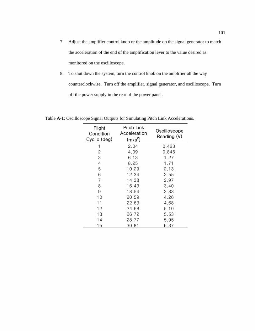
101
7. Adjust the amplifier control knob or the amplitude on the signal generator to match
the acceleration of the end of the amplification lever to the value desired as
monitored on the oscilloscope.
8. To shut down the system, turn the control knob on the amplifier all the way
counterclockwise. Turn off the amplifier, signal generator, and oscilloscope. Turn
off the power supply in the rear of the power panel.
Table A-1: Oscilloscope Signal Outputs for Simulating Pitch Link Accelerations.
FlightCondition
Cyclic (deg)
Pitch LinkAcceleration
(m/s2)
OscilloscopeReading (V)
1 2.04 0.4232 4.09 0.8453 6.13 1.274 8.25 1.715 10.29 2.136 12.34 2.557 14.38 2.978 16.43 3.409 18.54 3.8310 20.59 4.2611 22.63 4.6812 24.68 5.1013 26.72 5.5314 28.77 5.9515 30.81 6.37

102
Appendix B
Application of Energy Harvester
The final application of the energy harvester would be to power a sensor, most likely a
strain gauge that could monitor the loads that the part has seen. The sensor would have to
continuously take data and then process it into something useful to be wirelessly transmitted for
further processing and interpretation. This way, the actual loads the part experiences would be
used to determine component retirement times. The first step in processing the data is to use a
method called rainflow counting to reduce seemingly random data into something that is useful
and can be interpreted. Once the data has been rainflow counted, the fatigue damage can then be
calculated. A demonstration done at LORD Corporation by KCF Technologies obtained 53 sets
of 30 second strain data off of a lead-lag damper that was put into a quality test stand and put
through different flight conditions that ranged from mild to severe.
A.1 Rainflow Counting
Rainflow counting takes a random set of time history data, like stress or strain data, and
places it into histograms that express the amplitude and frequency of the cycles. It is the most
popular form of cycle counting today and the first necessary step in computing the fatigue
damage incurred by a part [26]. Before the data can be rainflow counted, the maxima and
minima must first be extracted. The strain data taken from the lead-lag damper and the extracted
maxima and minima are shown in Figure A-1.

103
The extracted maxima and minima are then put through the rainflow cycle counting
algorithm that puts the data into histograms of number of cycles of strain at their amplitudes.
Figure A-2 is a 3-D histogram that plots number of cycles versus amplitude versus mean value.
0 200 400 600 800 1000 1200-2
-1
0
1
2
3
4
5
6x 10
-5 Strain Time History
Data Points
Str
ain
0 50 100 150 200 250 300-2
-1
0
1
2
3
4
5
6x 10
-5 Extracted Maxima and Minima
Data Points
Str
ain
: m
ax a
nd m
in
Figure A-1: Strain Data from Lead-Lag Damper and the Extracted Maxima and Minima. The second
graph contains the maximum and minimum extracted data points from the strain time history. This data
can now be rainflow counted and put into a histogram that is useful for computing fatigue damage.
0.51
1.52
2.53
x 10-5
1.5
2
2.5
3
3.5
x 10-5
0
5
10
15
X - ampl
Rain Flow Matrix
Y - mean
num
ber
of
cycle
s
Figure A-2: Three Dimensional Histogram of Rainflow Counted Strain Data. The three
dimensional histogram contains data broken into amplitude of the cycle, mean value of the cycle,
and the number of cycles in each bin.
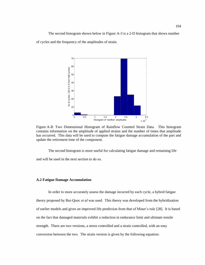
104
The second histogram shown below in Figure A-3 is a 2-D histogram that shows number
of cycles and the frequency of the amplitudes of strain.
The second histogram is more useful for calculating fatigue damage and remaining life
and will be used in the next section to do so.
A.2 Fatigue Damage Accumulation
In order to more accurately assess the damage incurred by each cycle, a hybrid fatigue
theory proposed by Bui-Quoc et al was used. This theory was developed from the hybridization
of earlier models and gives an improved life prediction from that of Miner’s rule [28]. It is based
on the fact that damaged materials exhibit a reduction in endurance limit and ultimate tensile
strength. There are two versions, a stress controlled and a strain controlled, with an easy
conversion between the two. The strain version is given by the following equation:
0 0.5 1 1.5 2 2.5 3 3.5
x 10-5
0
10
20
30
40
50
60
70
Histogram of "rainflow" amplitudes
Nr
of
cycle
s:
132.5
(7.5
fro
m h
alf-c
ycle
s)
Figure A-3: Two Dimensional Histogram of Rainflow Counted Strain Data. This histogram
contains information on the amplitude of applied strains and the number of times that amplitude
has occurred. This data will be used to compute the fatigue damage accumulation of the part and
update the retirement time of the component.
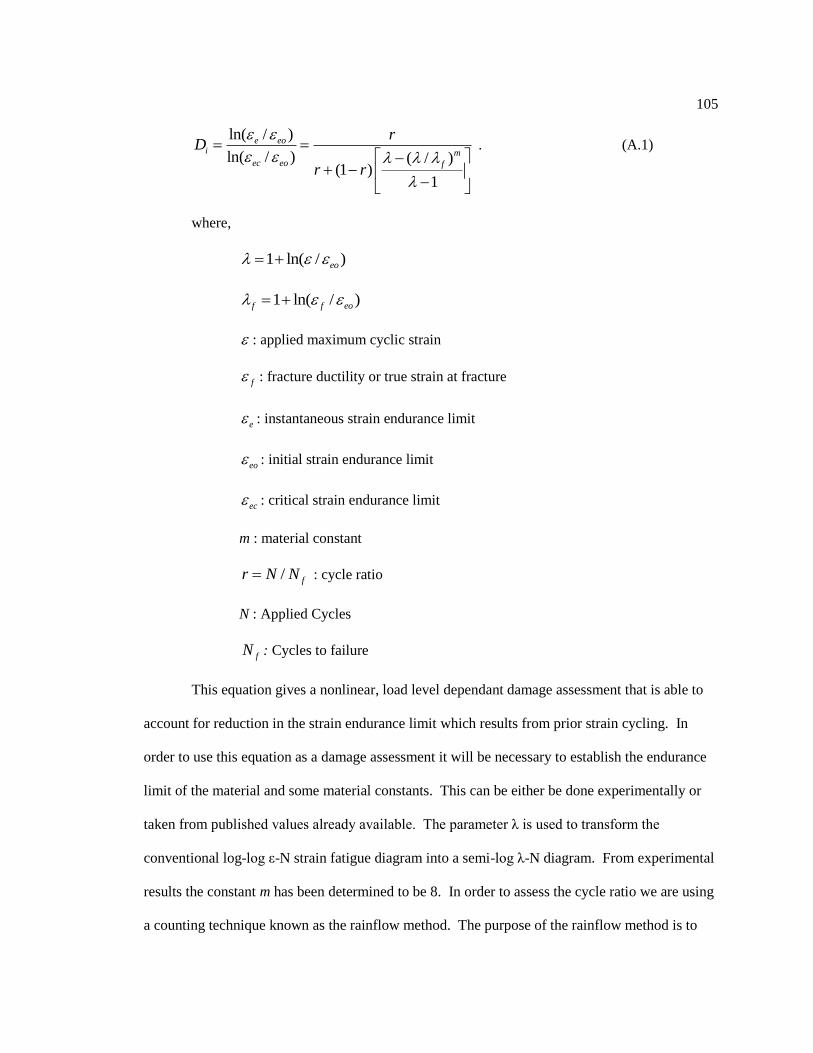
105
ln( / )
ln( / ) ( / )(1 )
1
e eoi m
ec eo f
rD
r r
. (A.1)
where,
1 ln( / )eo
1 ln( / )f f eo
: applied maximum cyclic strain
f : fracture ductility or true strain at fracture
e : instantaneous strain endurance limit
eo : initial strain endurance limit
ec : critical strain endurance limit
m : material constant
/ fr N N : cycle ratio
N : Applied Cycles
fN : Cycles to failure
This equation gives a nonlinear, load level dependant damage assessment that is able to
account for reduction in the strain endurance limit which results from prior strain cycling. In
order to use this equation as a damage assessment it will be necessary to establish the endurance
limit of the material and some material constants. This can be either be done experimentally or
taken from published values already available. The parameter λ is used to transform the
conventional log-log ε-N strain fatigue diagram into a semi-log λ-N diagram. From experimental
results the constant m has been determined to be 8. In order to assess the cycle ratio we are using
a counting technique known as the rainflow method. The purpose of the rainflow method is to
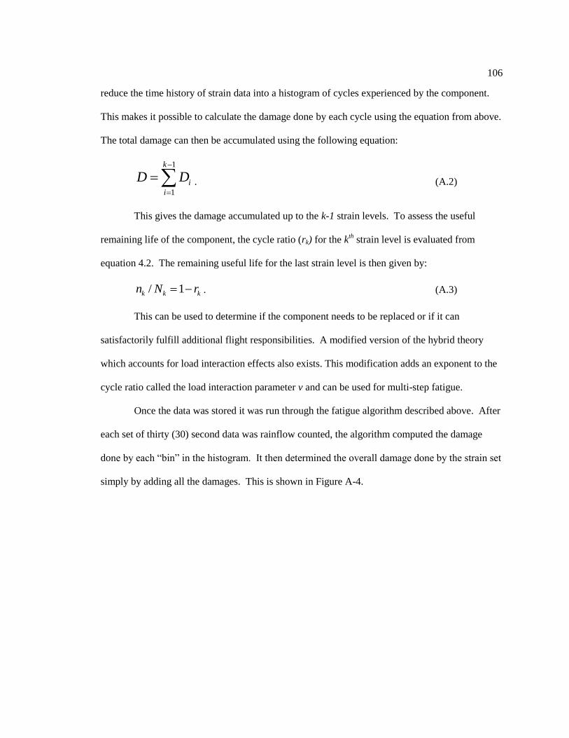
106
reduce the time history of strain data into a histogram of cycles experienced by the component.
This makes it possible to calculate the damage done by each cycle using the equation from above.
The total damage can then be accumulated using the following equation:
1
1
k
i
i
D D
. (A.2)
This gives the damage accumulated up to the k-1 strain levels. To assess the useful
remaining life of the component, the cycle ratio (rk) for the kth strain level is evaluated from
equation 4.2. The remaining useful life for the last strain level is then given by:
/ 1k k kn N r . (A.3)
This can be used to determine if the component needs to be replaced or if it can
satisfactorily fulfill additional flight responsibilities. A modified version of the hybrid theory
which accounts for load interaction effects also exists. This modification adds an exponent to the
cycle ratio called the load interaction parameter v and can be used for multi-step fatigue.
Once the data was stored it was run through the fatigue algorithm described above. After
each set of thirty (30) second data was rainflow counted, the algorithm computed the damage
done by each “bin” in the histogram. It then determined the overall damage done by the strain set
simply by adding all the damages. This is shown in Figure A-4.
107
After each set of data, a remaining life was calculated that showed how much longer the
part would last given the previous loading history. This is given as a percentage of life remaining
and is shown in Figure A-5.
0 10 20 30 40 50 600
0.5
1
1.5x 10
-3 Damage
Sampled period
Dam
age
Accumualated
Individual
Figure A-4: Individual and Accumulated Damage from Hybrid Theory Fatigue Algorithm. This
is the fatigue damage the part has accumulated according to the Hybrid fatigue theory.
0 10 20 30 40 50 600.9994
0.9995
0.9996
0.9997
0.9998
0.9999
1Remaining Life
Sampled Period
% o
f R
em
ain
ing L
ife
Figure A-5: Remaining Life from Hybrid Theory Fatigue Algorithm. This is the remaining life
the part has left after each set of strain data is rainflow counted and put through the fatigue
algorithm.

108
The hybrid fatigue theory proposed by Bui Quoc et al is one of many fatigue damage
accumulation methods that has been proposed over many years. The original is Miner’s Rule and
although it is a linear rule that is not very accurate, it still has widespread acceptance due to no
other theory gaining popularity. Along with data taken experimentally in a lab, data taken from a
wireless, autonomous sensor placed on the aircraft could be used to make fatigue damage
accumulation theories such as Miners Rule or the Hybrid Theory more accurate.