an empirical evaluation of value at risk by scenario … · 2018-06-12 · 1 an empirical...
TRANSCRIPT

An Empirical Evaluation of Value at Risk by Scenario Simulation
March 2000
Peter A. Abken Financial Economist
Risk Analysis Division Comptroller of the Currency
OCC Economics Working Paper 2000-3 Abstract: Scenario simulation was proposed by Jamshidian and Zhu (1997) as a method to separate computationally intensive portfolio revaluations from the simulation step in VaR by Monte Carlo. For multicurrency interest rate derivatives portfolios examined in this paper, the relative performance of scenario simulation is erratic when compared with standard Monte Carlo results. Although by design the discrete distributions used in scenario simulation converge to their continuous distributions, convergence appears to be slow, with irregular oscillations that depend on portfolio characteristics and the correlation structure of the risk factors. Periodic validation of scenario-simulated VaR results by cross-checking with other methods is advisable. The views expressed are those of the author and not necessarily those of the Comptroller of the Currency. The author thanks Jon Frye and Michael Sullivan for helpful comments, but is responsible for any errors. E-mail: [email protected] ; telephone: 202-874-6167; fax: 202-874-5394.
1
An Empirical Evaluation of Value at Risk by Scenario Simulation
One major obstacle to using Monte Carlo simulation for Value at Risk (VaR) calculations
on large bank portfolios is the need to revalue a very large number of positions.
Jamshidian and Zhu (1997) propose scenario simulation as a method to drastically reduce
the computational burden. The key feature of this technique is the separation of
revaluation and simulation. Scenario simulation samples a fixed set of precomputed
“scenarios” using a Monte Carlo procedure. In contrast, as Jamshidian and Zhu (JZ) put
it, standard Monte Carlo involves an “extortionate” number of portfolio revaluations.
While rapid advances in computing speed may eventually obviate the need for
approximation techniques, such approximations are widely used at financial institutions
today. It is common for such institutions to rely on different valuation models for
computing VaR from those used in the “front-office” system for pricing and hedging. The
former models generally have simple closed-form formulas, whereas the latter may use
numerically intensive lattice, Monte Carlo, or finite difference solutions for prices and
other outputs. Risk management practice is also moving toward more timely and frequent
VaR reports, such as intra-day VaR. In addition, since January 1, 1998, the banking
regulatory agencies have required capital to be charged against market-risk exposures in
trading portfolios held by banks that meet certain criteria.1 The charge is determined by
the daily computation of VaR based on a bank’s own internal model.
1The risk-based capital regulations are contained in the Federal Register, September 6, 1996 (Volume 61, Number 174) [61 FR 47357 12 CFR Part 3, 208, 225, 325 - Joint Final Rule: Risk-Based Capital Standards: Market Risk]. The rule was issued jointly by the Office of the Comptroller of the Currency, the Board of Governors of the Federal Reserve System, and the Federal Deposit Insurance Corporation. Compliance has

2
The examples in Jamshidian and Zhu give some evidence that scenario simulation
approximations are accurate. These examples include 10-year currency and interest rate
swaps, a 5-year interest rate floor, and a 5 5× interest-rate receiver’s swaption.2 Because
these instruments have long-term tenors, convexity effects for the options-based
instruments are minor. VaR at the 97.5 and 99.0 percent levels are reported only for the
swaps, whereas the floor and swaption examples are limited to mean, standard deviation,
and extrema of the 30-day horizon value. The scenario simulated values are within 2
percent of the Monte Carlo values.
The purpose of this paper is twofold: first, to detail the steps involved in doing
scenario simulation and to show its relationship with standard Monte Carlo and principal
component simulation; and, second, to evaluate the relative performance of these three
methods on several test portfolios. The precise meaning of “scenario” is defined below.
The empirical focus of the paper is on LIBOR-based option portfolios, in which
convexity effects are more pronounced than those found in JZ’s long-dated instruments.
JZ’s examples are also based on LIBOR derivatives.
The results indicate that the relative performance of scenario simulation on nonlinear
portfolios deteriorates compared with alternative approaches. Low dimensional
discretizations of the risk factor inputs can give poor estimates of VaR for linear and
nonlinear portfolios. The quality of the approximation depends on the extent of
nonlinearity in a portfolio. Furthermore, the tests described below demonstrate that
convergence of scenario simulation VaR results to benchmark values is slow as the
been mandatory since January 1, 1998, for banks whose trading activity [gross sum of trading assets and liabilities on a worldwide consolidated basis] equals: 10 percent or more of total assets; or $1 billion or more. However, the banking regulators have discretion in deciding which banks must comply. 2 The swaption is a 5-year option on a 5-year swap which comes into being if the option is exercised.
3
discretization gets finer. Although scenario simulation appears to be a useful alternative
to other, more computationally intensive methods, periodic validation of scenario-
simulated VaR results by cross-checking with other methods is advisable.
Alternative approaches to accelerating VaR by Monte Carlo have been proposed.
Picoult (1997) develops an extension of a Taylor series approach that relies on “grids of
factor sensitivities.” In contrast to the local approximation of a Taylor series, factor
sensitivities are the derivatives of the instrument value with respect to the risk factor
evaluated along a discrete set of values of a risk factor. Before running a VaR, these
sensitivities, including first, second, and higher order derivatives, including possibly
cross derivatives, are computed and stored, and then subsequently, in the VaR simulation,
changes in portfolio value are calculated by interpolation based on the stored factor
sensitivities. The user decides how many and what type of terms to include in the
approximation. Frye (1997) proposes a conservative approximation to VaR that is
predicated on a discrete scenario analysis rather than a Monte Carlo. He defines principal
component-based scenarios using a small set of large, prespecified shocks to the risk
factors, such as 2.33 standard deviations for a 99th percentile VaR. The greatest loss that
results in the process of revaluing a portfolio to these shocks is recorded as the VaR. Frye
(1998) suggests a Monte Carlo approach based on a stored multidimensional grid of
portfolio values as a function of a multidimensional grid of shocks to principal
components. Simulation proceeds by revaluing the portfolio by linearly interpolating
along the precomputed grid of portfolio values with respect to Monte Carlo draws for the
risk factors.
4
The final paper related to JZ is Reimers and Zerbs (1998), who use simple, multi-
currency portfolios of fixed-rate government bonds to assess the impact of the principal
component stratification technique proposed by JZ. This method is described in detail in
the following sections. They conclude that the relative difference in VaR based on the
full covariance matrix versus the stratified principal component covariance matrix is on
the order of one percent.
Sections 1, 2, and 3 review standard “brute-force” Monte Carlo, principal component
Monte Carlo, and scenario simulation, respectively. Most of the exposition focuses on
scenario simulation. Section 4 discusses the construction of test portfolios of LIBOR-
derivatives, and section 5 compares the simulation results on these portfolios for all three
methods. Section 6 gives concluding observations.
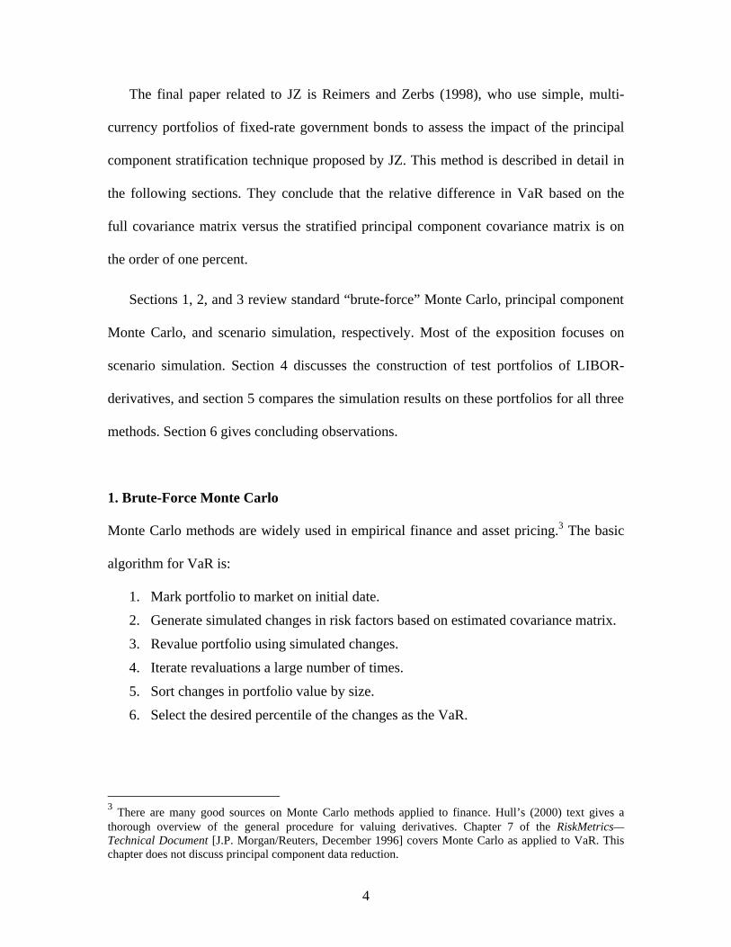
1. Brute-Force Monte Carlo
Monte Carlo methods are widely used in empirical finance and asset pricing.3 The basic
algorithm for VaR is:
1. Mark portfolio to market on initial date.
2. Generate simulated changes in risk factors based on estimated covariance matrix.
3. Revalue portfolio using simulated changes.
4. Iterate revaluations a large number of times.
5. Sort changes in portfolio value by size.
6. Select the desired percentile of the changes as the VaR.
3 There are many good sources on Monte Carlo methods applied to finance. Hull’s (2000) text gives a thorough overview of the general procedure for valuing derivatives. Chapter 7 of the RiskMetrics—Technical Document [J.P. Morgan/Reuters, December 1996] covers Monte Carlo as applied to VaR. This chapter does not discuss principal component data reduction.
5
A frequently insurmountable roadblock to using this algorithm on large portfolios is that
each Monte Carlo draw for the risk factors requires revaluation of all securities in the
portfolio. A second-order Taylor series (delta-gamma) approximation for the portfolio
value can be used to avoid the burden of full revaluation. However, such approximations
may perform poorly in VaR applications for portfolios that contain free-standing or
embedded out-of-the-money options, which would be missed by a local approximation.
2. Principal Component VaR
Principal component (PC) VaR reduces the computational burden by compressing the
number of risk factors through the use of a reduced set of principal components. Fewer
random numbers need to be drawn; however, the principal components must be inverted
back into the original number of risk factors in order to revalue the portfolio. The VaR
algorithm is the same as that for brute-force Monte Carlo, except for the addition of the
computation of the principal components and the inversion process.4
By construction, principal components are uncorrelated. The principal components
for the test portfolios are derived from the covariance matrix of the monthly log changes
in a set of “key” interest rates along the yield curve. A complete discussion of the data
construction appears below. Let the interest rate risk factors be given by the 1n × vector
RF and evolve through one discrete time step as
(1) ( )1 0exp=RF RF u ,
where the shocks ~ (0, )N Qu .
4 Recent references on principal component VaR are Singh (1997) and Kreinin et al. (1998). Singh’s examples use a Taylor series approximation to the pricing function rather than full revaluation.

6
The covariance matrix Q is factored into a diagonal matrix of eigenvalues Λ and an
orthogonal matrix of eigenvectors [ ]nE e e= 1L :
(2) .EQE′Λ =
Both the eigenvalue and eigenvector matrices are truncated to m n< columns in order to
include only a subset of the largest eigenvalues and their associated eigenvectors. The
shock vector u is generated by a linear combination of standard normal shocks
~ (0, )mN Iη :
(3) 1m mn m m
E η×× ×
′= Λu ,
where the principal components are ηΛ . PC simulation consequently entails using a
covariance matrix approximation for the full n n× covariance matrix.
In LIBOR derivative portfolios examined below, four principal component risk
factors are retained from the original eight key-rate risk factors per market. These account
for over 97 percent of the total variance of the original data (as measured in the standard
way by the ratio of the sum of the eigenvalues of the four components to the sum of all
the eigenvalues).
3. Scenario Simulation
The mechanics of scenario simulation are quite different from the other types of Monte
Carlo applied to VaR because of the separation of the revaluation stage from the
simulation stage.
The core step in scenario simulation is the approximation of the multivariate normal
distribution by the binomial distribution. The joint occurrence of particular discrete states

7
of the risk factors constitutes a “scenario.” Such discrete approximations are conventional
in statistics, but their incorporation into a simulation analysis, and particularly the
“stratified” discretization discussed below, make the JZ approach a novel way to
calculate VaR.
Principal component analysis is treated as a necessary adjunct to scenario simulation
because the number of scenarios becomes huge even for a relatively small number of risk
factors. JZ note that with 12 key rates in a yield curve model and an assumption that each
can take three possible values, the total number of scenarios is 123 531,441= . With five
states for each variable, the total number of scenarios explodes to more than 200 million.
The use of principal component analysis can dramatically reduce the number of scenarios
with relatively little sacrifice of accuracy because interest rate movements tend to be
highly correlated. Even with principal components standing in for market factors, the
number of scenarios for portfolios involving term structures in more than just a few
currencies can number in the trillions. Further assumptions must be made on the structure
of the covariance matrix of the risk factors to pare down the problem into one of
manageable proportions. The large number of scenarios requires a Monte Carlo
procedure to compute VaR, instead of a direct calculation based on the full set of
scenarios and their associated probabilities of occurrence. These procedures are explained
below, reproducing JZ’s equations (15)–(17) and adding some further explanatory detail.
There are assumed to be 1m + states, ordered from 0 to m , with probabilities
determined in the conventional way for the binomial:
(4) !
Probability( ) 2 , 0, ,!( 1)!
m mi i m
i m−= ⋅ =
−L .

8
These probabilities are not explicitly calculated or used in scenario simulation. They
enter the VaR calculation in the construction of the “lookup table” for scenarios. The
essence of scenario simulation is the discretization of continuously distributed random
variables that represent the principal components (linear transformations of the risk
factors). For example, if each principal component can be in five possible states, the total
number of states is 35 125= . These can be enumerated and the portfolio can be revalued
for each discrete shock. The key step is the mapping of a continuously distributed shock
into a discrete shock. Although normality is assumed, the method can be applied to other
distributions. The relationship between the normal and the binomial is given by
(5) 1 21 2 !exp , 0, ,
2 !( )!2
i
i
a m
a
x mdx i m
i m iπ
+ − − = = −
∫ L .
Starting from 0a = −∞ for the initial lower limit of integration, the next boundary point
1a that equates the area of the normal density to the binomial probability for the 0th
binomial state is determined numerically by any standard root-solving procedure. The
remaining upper limits of integration 1ia + , defining areas under the normal density curve
in the interval 1[ , ]i ia a + , are then found successively, state by state. For five states, these
values are:
(6) 1 2 3 41.53412; 0.48878; 0.48878; 1.53412a a a a= − = − = = .
A standard normal variate z drawn from a random number generator can then be mapped
into a discrete state by testing where it falls relative to the break points:
(7) ( )1( ) ifm
i iB z i a z a += ≤ < ,

9
where {0, , }i m∈ … . This mapping comes into play in two places: in the construction of
the lookup table of scenarios and in the simulation of scenarios.
Lookup Table Construction
The discrete variable ( )( )mB z , which represents a particular state, can be normalized as
(8) ( ) ( )( ) (2 ( ) ) /m mz B z m mβ = − ,
that is, the transformed random variable has mean 0 and variance 1 (the mean of the
binomial distribution is / 2m and the variance is / 4m ). This variable’s dependence on z
is not explicitly used in the lookup table construction. Rather, a set of shocks ( )( )m zβ is
defined based on the set of integers that the discrete variable B assumes. For 5 states
( 4)m = , the variable ( )( )mB z takes values {0,1, 2,3,4} and this translates into
normalized shocks ( )( )m zβ with possible values { 2, 1,0,1,2}− − .
The ( )( )m zβ values are the discrete values of z that are the primary ingredients for
constructing the lookup table. A matrix of scenario indexes is computed that exhausts all
possible state combinations. These discrete state values {0, , }i m∈ … for each principal
component are translated into the corresponding ( )( )m zβ , which in turn are plugged in as
simulated principal components. These in turn are inverted into realizations of the risk
factors that are used to revalue each instrument in each scenario. The resulting valuations
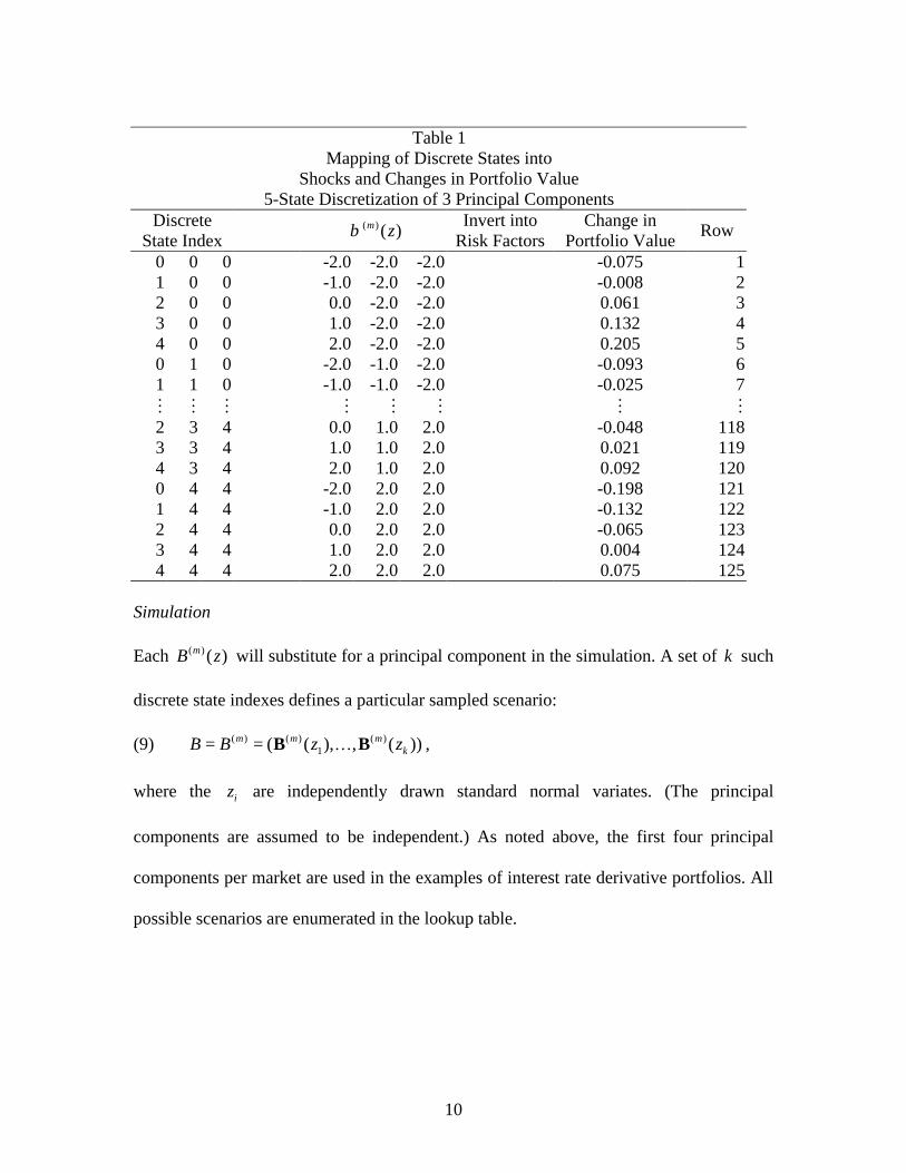
are stored for later use during the simulation. The following table illustrates the mapping
process using 5 states and a total of 125 possible scenarios.
10
Table 1
Mapping of Discrete States into Shocks and Changes in Portfolio Value
5-State Discretization of 3 Principal Components Discrete
State Index ⇒ ( )( )m zβ
Invert into Risk Factors
Change in Portfolio Value
Row
0 0 0 ⇒ -2.0 -2.0 -2.0 ⇒ -0.075 1 1 0 0 ⇒ -1.0 -2.0 -2.0 ⇒ -0.008 2 2 0 0 ⇒ 0.0 -2.0 -2.0 ⇒ 0.061 3 3 0 0 ⇒ 1.0 -2.0 -2.0 ⇒ 0.132 4 4 0 0 ⇒ 2.0 -2.0 -2.0 ⇒ 0.205 5 0 1 0 ⇒ -2.0 -1.0 -2.0 ⇒ -0.093 6 1 1 0 ⇒ -1.0 -1.0 -2.0 ⇒ -0.025 7 M M M M M M M M 2 3 4 ⇒ 0.0 1.0 2.0 ⇒ -0.048 118 3 3 4 ⇒ 1.0 1.0 2.0 ⇒ 0.021 119 4 3 4 ⇒ 2.0 1.0 2.0 ⇒ 0.092 120 0 4 4 ⇒ -2.0 2.0 2.0 ⇒ -0.198 121 1 4 4 ⇒ -1.0 2.0 2.0 ⇒ -0.132 122 2 4 4 ⇒ 0.0 2.0 2.0 ⇒ -0.065 123 3 4 4 ⇒ 1.0 2.0 2.0 ⇒ 0.004 124 4 4 4 ⇒ 2.0 2.0 2.0 ⇒ 0.075 125
Simulation Each ( )( )mB z will substitute for a principal component in the simulation. A set of k such
discrete state indexes defines a particular sampled scenario:
(9) ( ) ( ) ( )1( ( ), , ( ))m m m
kB B z z= = B B… ,
where the iz are independently drawn standard normal variates. (The principal
components are assumed to be independent.) As noted above, the first four principal
components per market are used in the examples of interest rate derivative portfolios. All
possible scenarios are enumerated in the lookup table.
11
The discretization of any draw from a “continuous” random number generator on a
computer is assigned to an element of the discrete vector of shocks.5 The probability of
the occurrence of any particular draw for ( )( )mB z (given by equation (4)) is implicitly
captured by the process of sorting the draws of the continuous variable z into discrete
states as represented by equations (5) and (7). For independent principal components, the
joint probability of a scenario—a combination of discrete variables represented by
equation (9)—is the product of probabilities of each individual discrete variable. (The
general case of correlated discrete variables is discussed subsequently.) In other words,
the simulation samples with replacement from the scenarios in the lookup table. The
frequency of the sampling of any given scenario is in proportion to its discrete
probability.
A synopsis of the scenario simulation algorithm is:
1. Construct the lookup table by enumerating all possible scenarios involving the
predefined states for each principal component or risk factor.
2. Compute ( )( )m zβ for each principal component or risk factor in a given scenario.
3. Compute the corresponding risk factors for each scenario (see equations (13) and (14) below).
4. Revalue each instrument in the portfolio using the risk factors for each scenario. Compute the change in portfolio value from its initial value. Assign an index number (the row number in the table) to the change in portfolio value based on a given scenario.
5. Simulate by drawing independent normal random variates z and map them into the states ( )( )mB z .
6. Scan the lookup table for the corresponding scenario and return the precomputed change in portfolio value and store it.
5 Of course, any computer-based random number generator is also discrete, given the finite number of integers that can be represented as a 32-bit integer, based on current system constraints. Still, typical linear congruential generators can create at least 2 billion unique random numbers, and many can crank out vastly more than this (at the cost of being slower in execution) before they start to repeat their cycle. See Dwyer (1995).

12
7. Repeat simulation steps (5) and (6) a large number of times.
8. Sort the vector of simulated changes in portfolio value by size and evaluate the desired percentile value for the VaR.
In contrast with standard Monte Carlo or principal component Monte Carlo, the
number of portfolio revaluations is independent of the number of simulation iterations
under scenario simulation. Although the discretization limits the sampling from a given
risk factor’s distribution, the joint probabilities across risk factors can be very low. In the
example given here, the principal components are independent. For example, in the 5
state example, while the smallest probability for one variable is 1/16 0.0625= , the
smallest joint probability is 3(1/16) 0.0002= . Nevertheless, for portfolios with
sufficiently nonlinear payoffs, the failure to sample far enough into the tails may result in
material inaccuracies of the scenario simulation approximation. The same may be true of
extreme positions in digital options or other options positions that create spikes that the
discretization misses.
Stratification of Principal Components JZ propose a stratification of principal components to handle multimarket, multi-currency
portfolios. Principal components are computed for a given market, say, for the term
structure in a given currency, and consequently individual markets retain a distinct
identity in the simulation. Although mutually uncorrelated for interest rates in a given
currency, the principal components have correlations with principal components of
interest rates in other currencies, as well as with other risk factors, such as foreign
exchange rates.

13
However, even with the reduction in dimension gained through the use of principal
components, there still can be trillions of scenarios to reckon with in multicurrency,
multimarket portfolios. The number of dimensions for the scenario simulation could
easily explode out of hand, wiping out its advantage over conventional Monte Carlo. For
example, the total number of scenarios in the multicountry portfolios examined below is
123.4 10× for the 7-state discretization and 154.7 10× for the 11-state discretization.6 The
solution to the dimensionality problem is simply to use Monte Carlo to simulate the
discrete joint distribution of the risk factors. Scenarios need to be tabulated only within
each currency block.
Dealing with dependent discrete joint random variables is straightforward. Let sQ be
the covariance matrix based on the stratified decomposition of risk factors into principal
components. Generating correlated standard random normal variates follows the usual
procedure for Monte Carlo. A factorization of the covariance matrix sQ is used to create
a vector of correlated shocks X from the vector z of uncorrelated standard normal
variates, such that
(10) 1( , , ) ~ (0, ).n sX X X N Q= …
The discrete scenarios (9) use X in place of z: (11) ( ) ( ) ( )
1( ( ), , ( ))m m mnB B X X= = B B… .
Otherwise, scenario simulation proceeds exactly as given in the synopsis above. JZ
formally prove the convergence of the multinomial approximation given by (11) to the
continuously distributed random vector (10).
6 This is computed by
( ) ( ) ( )( )3
# states per $ yield curve factor # states per foreign yield curve factor # states per exchange rate .× ×

14
As JZ note, premultiplying the B matrix derived from uncorrelated normal variates by
the Cholesky factor of sQ to induce the desired covariance structure would scramble the
stratification. To avoid this loss of information, the Cholesky factor is applied to create
the X vector in (10) before discretization.
4. Test Portfolios Four kinds of multicurrency, LIBOR-derivatives portfolios are constructed to compare
standard Monte Carlo, principal component Monte Carlo, and scenario simulation. Each
type of portfolio was designed to contain one type of instrument: swaps, caps/floors,
caplets/floorlets, and swaptions. Such derivatives represent an important share of most
large banks’ trading portfolios, and typically trading books are organized into
subportfolios by instrument type.
Data
All portfolios involve swap or option positions on four currencies: the U.S. dollar,
German mark, Swiss franc, and British pound. The exchange rate and interest rate data
were obtained from the Bloomberg History Tool and are end-of-day Wednesday
observations. The data sample period runs from December 1, 1993 to November 25,
1998, totaling 261 observations per time series. The use of Wednesday observations
minimized the number of missing observations in the data set. There were eight missing
Wednesday observations across all countries for interest rates or FX. These dates were
backfilled using observations from the day before.
Spot LIBOR at maturities of 3, 6, 9, and 12 months and swap rates at maturities of 2,
5, 7, and 10 years were used to derive forward LIBOR curves. These maturities constitute
the key rate maturities. Standard Granger causality tests, reported in the appendix,
15
indicate that daily spot swap rates Granger-cause daily spot LIBOR rates, but not the
converse. To mitigate potential distortion to measured correlations of daily changes in
rates, weekly changes in risk factors, and hence a weekly holding period for the VaR, was
employed in the simulations.7
All derivatives considered in this study have quarterly resets. Linear interpolation was
used to fill out points along the yield curve: 8 key rates were expanded into 40 rates at
quarterly maturity intervals out to 10 years.8 Spot swap rates with maturity less than 2
years were derived from the spot LIBOR rates. In turn, daily 3-month forward LIBOR
curves in each currency were derived from the spot swap rate curve.9
The forward LIBOR curve was used to construct a discount bond price curve and
corresponding yield curve. Yields are more compactly represented in a principal
component decomposition and are less contaminated by noise than are forward rates.
Yields are the variables that get simulated in the VaR calculations. Bond prices are
needed as inputs into the Black model for pricing interest-rate derivatives.
Covariance Matrix
The five-year data sample is subdivided into five subsamples, each spanning one year
starting with the first Wednesday in December. This choice was motivated by the Basle
Committee for Banking Supervision’s internal models approach for setting regulatory
7 The general issue of data nonsynchroneity is discussed in RiskMetrics (RM Data Sets.pdf), section 8.5. Strips of Eurodollar futures rates for intermediate tenors are often used in constructing LIBOR curves. See Overdahl et al. (1997). 8 Linear interpolation of a small set of key rates is a problematic practice because the resulting forward curve takes a saw-tooth shape. A difference in liquidity between the interbank deposit market (the spot LIBOR rates) and the swap market may also contribute to a jump in the derived forward LIBOR curve where the two maturity segments join. See Wang (1994). 9 Formulas and conventions for LIBOR-based derivatives are described in Rebonato (1998) and Musiela and Rutkowski (1997).
16
capital for trading portfolios.10 (The U.S. banking regulations for using VaR for capital
determination, which derive from the Basle framework, stipulate that no less than one
year’s worth of daily data be incorporated into the covariance matrix and that a given
yield curve incorporate no fewer than six “segments” of the curve “to capture differences
in volatility and less than perfect correlation of rates along the yield curve.”11)
The full covariance matrix consists of interest rate and foreign exchange rate blocks
of risk factors: the yield curve key rates from each country and their exchange rates,
giving a total of 31 factors. A stratified principal component decomposition of each yield
curve, retaining the four largest factors, reduced the dimension of the covariance matrix
to 19 19× . The first four principal components captured at least 97 percent of the total
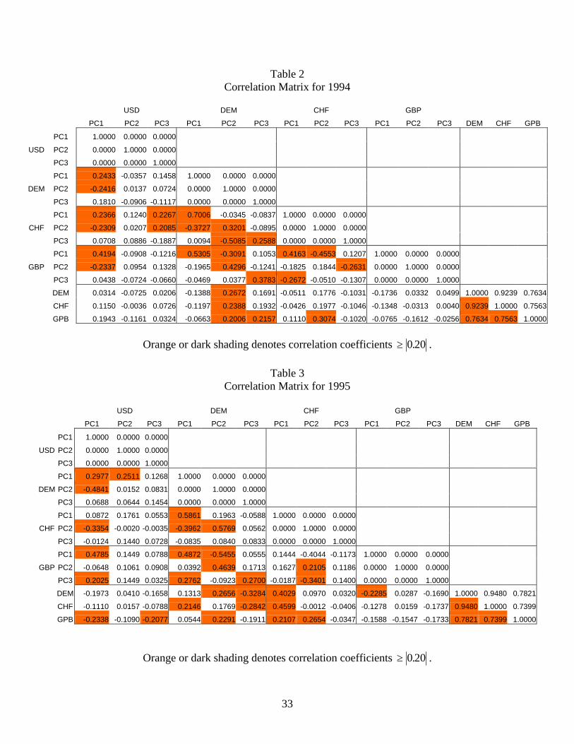
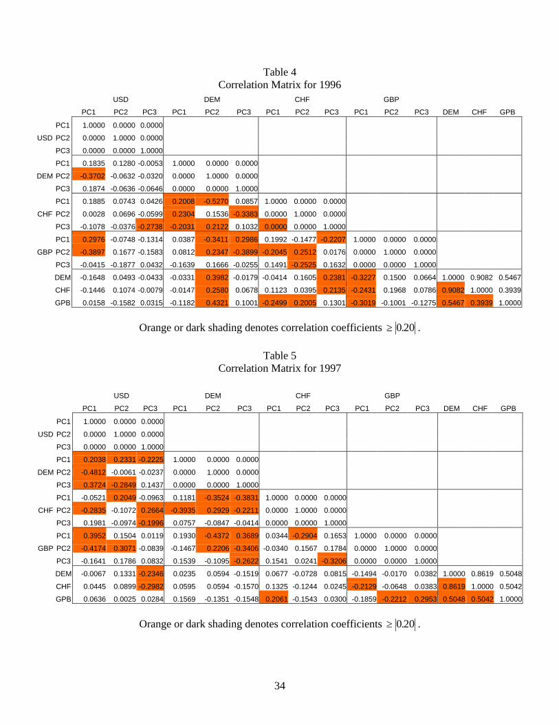
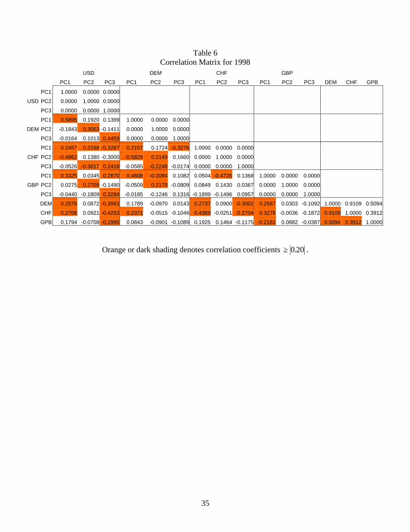
variation in the interest rate data in each currency. Tables 2–6 show the stratified
correlation matrix for 1995–1998, respectively, where correlations for the first three
interest rate PCs are displayed to conserve space. The currency labels are USD, DEM,
CHF, and GBP, denoting the U.S., Germany, Switzerland, and U.K, respectively. The
transformation of the original covariance matrix into the stratified matrix is similar to the
standard decomposition of a covariance matrix in (2). The off-diagonal blocks, such as
the covariance of DEM principal components with USD principal components, are
computed by pre- and post-multiplying the original covariance matrix block by the DEM
and USD blocks of eigenvector matrices, respectively. The main diagonal of own-country
interest rate principal component blocks are identity matrices since principal components
are orthonormal. However, the off-diagonal blocks show a pattern of correlations
between countries that exhibits a degree of stability from year to year.
10 Basle Committee on Banking Supervision, “Amendment to the Capital Accord to Incorporate Market Risk,” January 1996.

17
The tables indicate correlations greater than 0.20 in absolute value in dark shading.
The cross-correlations of PCs in the off-diagonal blocks tend to show positive correlation
of corresponding PCs—for example, first USD PC with first DEM PC. The results are
variable from year to year, with 1998 having the greatest correlations and 1997 the
weakest.
Exchange rate–interest rate principal component correlations, though strong at times
(such as the first Swiss interest rate PC versus FX rates in 1995), are much more erratic.
However, the FX block has high cross-rate FX correlation every year.
Portfolio Construction
An arbitrary set of positions in each instrument is assumed for each currency. The
basic portfolios are designed to investigate nonlinear payoffs, the classic inverted “U” of
a negative gamma exposure. As in any Monte Carlo exercise, the results do not
necessarily generalize. They are valid for the particular portfolios being examined.
However, qualitatively similar results were obtained for other test portfolios, which are
not reported here to conserve space.
The portfolios consist of identical positions in derivatives in each currency that have
identical U.S. dollar notional value ($10,000) at the initial date. The four types of
portfolios are:
1. 10-year pay-fixed/receive floating swaps at current market rates.
2. 6-year caps and floors. At-the-money long cap and long floor (that is, strikes are set equal to the current forward LIBOR curve). Short out-of-the-money caps and floors with strikes set equal to exp( 3 )T TL σ± , where T is the reset date of a
caplet, TL is forward LIBOR for time T , and Tσ is the volatility of forward LIBOR for a weekly holding period. The notional value of the out-of-the-money positions is twice that of the at-the-money positions.
11 See footnote 1.
18
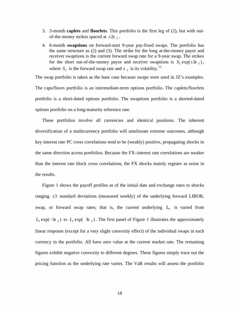
3. 3-month caplets and floorlets. This portfolio is the first leg of (2), but with out-of-the-money strikes spaced at 2 Tσ± .
4. 6-month swaptions on forward-start 9-year pay-fixed swaps. The portfolio has the same structure as (2) and (3). The strike for the long at-the-money payor and receiver swaptions is the current forward swap rate for a 9-year swap. The strikes for the short out-of-the-money payor and receiver swaptions is exp( 3 )T TS σ± ,
where TS is the forward swap rate and Tσ is its volatility.12
The swap portfolio is taken as the base case because swaps were used in JZ’s examples.
The caps/floors portfolio is an intermediate-term options portfolio. The caplets/floorlets
portfolio is a short-dated options portfolio. The swaptions portfolio is a shorted-dated
options portfolio on a long-maturity reference rate.
These portfolios involve all currencies and identical positions. The inherent
diversification of a multicurrency portfolio will ameliorate extreme outcomes, although
key interest rate PC cross correlations tend to be (weakly) positive, propagating shocks in
the same direction across portfolios. Because the FX–interest rate correlations are weaker
than the interest rate block cross correlations, the FX shocks mainly register as noise in
the results.
Figure 1 shows the payoff profiles as of the initial date and exchange rates to shocks
ranging 3± standard deviations (measured weekly) of the underlying forward LIBOR,
swap, or forward swap rates; that is, the current underlying TL is varied from
exp( 3 )T TL σ− to exp( 3 )T TL σ+ . The first panel of Figure 1 illustrates the approximately
linear response (except for a very slight convexity effect) of the individual swaps in each
currency in the portfolio. All have zero value at the current market rate. The remaining
figures exhibit negative convexity to different degrees. These figures simply trace out the
pricing function as the underlying rate varies. The VaR results will assess the portfolio

19
performance as simulated interest rate and currency shocks hit these portfolios over the
weekly holding period. A volatility shock could also readily be included as an additional
risk factor in each market, but the focus of this study is on “price” risk, as in JZ.
Risk Factor Simulation
Following the examples in JZ, risk factors are simulated as lognormal processes.
Incorporating other continuous distributions for the risk factors is readily done using the
fractile-to-fractile mapping described in Hull and White (1998).
For the crude Monte Carlo simulation, the vector of risk factors RF at the one-week
horizon is generated by
(12) ( )0exp=RF RF u ,
where the vector of shocks ~ (0, )N Qu and is 35 1× . The risk factors are the eight key
rates along the yield curve for each country and three foreign exchange rates. For the
stratified principal component simulation, the vector is given by
(13) ( )0exp=RF RF u% ,
where
3 18 4 4 4 4 1USD USD USD DEM DEM DEM CHF CHF CHF GBP GBP GBP FXE E E Eη η η η
×× × ×
′ ′ ′ ′= Λ Λ Λ Λu u% ,
1 2x x denotes stacked vectors, and NE is the truncated eigenvector matrix for country N
that retains eigenvectors corresponding to the four largest eigenvalues of that country’s
yield curve. The interest rate principal components and FX rate shocks are
| | | ~ (0, )sUSD USD GBP GBP FX N Qη ηΛ Λ uL ,
12 A receiver swaption is a call on a swap; that is, the right to receive fixed and pay floating. A payor swaption is a put on a swap; that is, the right to pay fixed and receive floating.

20
where sQ is the 19 19× stratified covariance matrix. The main diagonal of the stratified
covariance matrix contains the (stratified) eigenvalues of the principal components and
its last three elements are the variances of the log changes in exchange rates.
Scenario simulation tabulates risk factors and corresponding changes in portfolio
value in a lookup table. The risk factor equation is equivalent to (13), except that the
vector of shocks u% is replaced by
(14) 3 18 4 4 4 4 1
ˆ USD USD USD DEM DEM DEM CHF CHF CHF GBP GBP GBP FXE B E B E B E B B×× × ×
′ ′ ′ ′= Λ Λ Λ Λu ,
where NB is a vector of standardized discrete shocks to country N’s yield curve that have
been stored as a particular scenario, as in the example displayed in Table 1, and FXB
contains standardized discrete shocks to the exchange rates. Separate lookup tables for
interest rate scenarios and corresponding changes in portfolio values are constructed for
each currency. FX rate changes are also tabulated in separate lookup tables. As discussed
above, Monte Carlo simulation is used to sample from the discretized joint distribution of
the risk factors. The correlated normal random variables X defined by (10) drives the
sampling from both interest rate and exchange rate scenarios, which translate the
discretized multicurrency portfolio value changes back into dollars.
Portfolio Valuation
The VaR evaluated in this study represents a ten-day exposure, measured from the
first business day of December for each year in the sample. Each portfolio is priced at the
initial date and fully revalued ten days later. On each draw, the simulated 8 yield risk-
factor values per currency are interpolated to a set of 40 yields, from 3 months to 10 years
at quarterly maturity intervals. The corresponding discount price curve is computed,

21
which provides the discount factors for all options-based instruments and from which is
derived spot and forward swap rates (for swaps and swaptions) or the forward LIBOR
curve (for caps and caplets).
Caps, floors, and swaptions are valued by the standard one-factor Black model.
Although once regarded as an inconsistent, ad hoc application of the Black-Scholes
model to interest rate derivatives, in recent years academic research has established that
the model is fully consistent and arbitrage-free when applied to single instrument classes,
such as caps or swaptions.13
In the examples below, a VaR run consists of 1,000 draws for Monte Carlo risk factor
vector (12) or principal components risk factor vector (13), and 10,000 draws for scenario
simulation vector (14), which drives the sampling from the joint discrete distribution for
the portfolio value changes. Although 1,000 draws is relatively small and inaccurate for
crude Monte Carlo (that is, without variance reduction techniques), this number is of the
same order of magnitude as the number of iterations that large banks use for Monte Carlo
and historical VaR simulation. Scenario simulation can be iterated to much higher
numbers for the same total CPU time as Monte Carlo; 10,000 iterations was arbitrarily
chosen. All of these runs are repeated 20 times and the means and standard errors of the
resulting VaRs are reported in Table 8.
Two discretization choices for four principal components were used for scenario
simulation: a coarse discretization of 7 5 3 3× × × , yielding 315 distinct scenarios for a
13 See Rebonato (1998) or Musiela and Rutkowski (1997). The Black model for interest rate derivatives can be derived as a single-factor, lognormal case of the Brace-Gatarek-Musiela (1995) model. The Black model is inconsistent across instruments, the most notable case being the model’s simultaneous assumption that forward LIBOR is lognormally distributed in valuing caps while forward swap rates are lognormally distributed in valuing swaptions. Nevertheless, this discrepancy is negligible compared to other sources of error in VaR calculations. Furthermore, most practitioners and some academics disregard the inconsistency in pricing and hedging applications (see Jamshidian (1997) and Derman (1996)).

22
single country’s yield curve, and a fine discretization of 11 7 5 5× × × , giving 1925
scenarios. The fine discretization is intended to sample deeper into the tails of the risk
factor distributions to approximate more accurately the convexity of the option portfolios.
Foreign exchange rate distributions were discretized into 7 states for both high and low-
density interest rate discretizations.
The results in the next section are based on crude Monte Carlo, principal component
Monte Carlo, and scenario simulation runs. The VaR outcome for each of the methods is
repeated 20 times to determine empirical distributions of the estimates for each method.
5. Test Portfolio VaR Results.
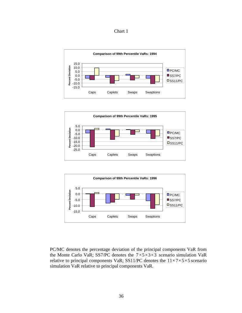
The simulation results are sensitive to time period and to type of portfolio. Chart 1
summarizes the output for the basic portfolios for the full four-currency portfolios. The
panels give a relative comparison of 99th percentile VaRs, based on averages of 20
simulation runs. Within the chart, each panel gives individual yearly results, for each type
of instrument portfolio (caps, caplets, swaps, and swaptions). The bars on the left show
the percentage deviation of the principal component VaR in relation to the Monte Carlo
VaR. The central bars indicate the comparison of the 7 5 3 3× × × scenario simulation
(SS7) with principal components taken as the benchmark, and the bars on the right
represent the comparison of the 11 7 5 5× × × scenario simulation (SS11) with principal
components.
At the 99th percentile level, the PC/MC comparison for swaps is in good agreement—
off by less than 1.5 percent, except for 1997 where the discrepancy is an underestimate
by PC of 7.5 percent. The PC/MC match is good for the nonlinear instruments, except for
caplets in 1996 and swaptions, for which a 5 percent gap exits in most years. Evidently,

23
the approximation error due to excluding higher order PCs as risk factors has a disparate
impact on the VaR outcomes, particularly for nonlinear instruments. The PC results are
taken as the benchmark for scenario simulation rather than the Monte Carlo results in
order to keep errors arising from discretization distinct from those stemming from PC
approximation of the risk factors.14
The deviations in Chart 1 tend to be in the same direction from year to year for each
instrument portfolio, with scenario simulation understating the VaR in relation to PC
simulation. These gaps can be substantial. The 1995 SS7 underestimates the VaR by over
20 percent and the SS7 swaption errors are consistently greater than 10 percent. The
discrepancy narrows only slightly in the SS11 results. In the case of the caps, the
deviation reverses sign and equals or exceeds 10 percent in 1994, 1997, and 1998. Table
7 gives the output in tabular form along with the corresponding 95th percentile results,
while Table 8 shows the dollar values of the VaRs and corresponding standard
deviations, as well as the standard error for the mean of the 20 VaR estimates. Generally,
the differences in outcomes across simulation runs, particularly for scenario simulation,
are statistically significant.
These results contrast with JZ’s, who find in their single currency swap examples that
scenario simulation VaRs (at the 97.5 and 99 percent confidence levels) differ by no
more than 2 percent from the Monte Carlo results. In their Table 6, JZ give an example of
14 Furthermore, one can argue that Monte Carlo is not the appropriate benchmark against which to judge the other results because Monte Carlo places too few restrictions on the way in which key rates can evolve through time. The covariance matrix only weakly constrains the way shocks hit the yield curve. Monte Carlo allows improbable movements in yields of different maturities in relation to one another, such as the 6-month and 2-year key rates rising sharply as the 1-year key rate falls. On the other hand, shocking principal components greatly limits the possible configuration of relative rate movements. However, low-order representations of the term structure, such as by two or three components, limit the possible movements and shapes too much. See Rebonato (1998), chapter 3. Another consideration is that the
24
a multicurrency interest rate swap portfolio, but they only report results for one
discretization that is sampled at different iteration levels and make no comparison to
Monte Carlo.
Accounting for Erratic Results
The variation in scenario simulation results in relation to the PC benchmarks appears to
be analogous to well-known behavior of binomial option pricing models—namely, as the
density of the approximating lattice decreases, the binomial model value oscillates more
widely around the true analytic price. A similar phenomenon may account for the
scattered values of the scenario simulation VaR around the PC benchmark. Simply
increasing the number of nodes by using a moderate number of time steps remedies the
oscillation problem for standard options. In contrast, the computational burden of
scenario simulation rapidly becomes excessive as the discretization of each state becomes
finer.
The size of the deviations induced by coarse discretizations of the risk factors and
their variation with finer discretizations is examined systematically in another simulation
exercise. The interest-rate derivatives portfolios above are too complex to use in a
computationally intensive convergence analysis. Instead, simplified linear and nonlinear
portfolios are used. The linear portfolio consists of two assets, with one unit of each.
Each unit is valued initially at par. Their prices are correlated and are lognormally
distributed. The VaR of the portfolio is determined by scenario simulation, with each
price (risk factor) distribution discretized into an equal number of odd-numbered states
ranging from 5 to 63. The nonlinear portfolio is similar to the interest rate caplet portfolio
excluded higher order PCs contain most of the errors in the data. Monte Carlo includes all sources of variation.
25
above, with out-of-the-money options spaced at two standard deviations from the at-the-
money price; instead of four currencies there are two prices. The constituent options are
priced by Black-Scholes as before.
Chart 2 displays the percentage deviation of the scenario simulation VaRs for the
linear portfolio, at both the 95th and 99th percentile levels, from the VaR computed by the
standard covariance method. The upper panel shows the outcome for zero correlation
between the two risk factors; the lower the results for a correlation of 0.5. Each 95th and
99th percentile VaR pair for a given discretization level was generated based on one
million scenario simulation draws. Virtually the same plot is reproduced if the
simulations are repeated—the deviations do not predominately represent random
“sampling variation.” The pattern varies with instrument portfolio and correlation
assumption.
Qualitatively, the two plots for the linear portfolio are similar: the most striking
aspect of these graphs is that the deviations oscillate in an irregular pattern as the
discretization becomes finer. Although the fluctuations diminish as the number of states
in a simulation run increases, they are still sizable—convergence is slow. For the coarse
discretization cases that would typically be used for scenario simulation, the deviations
can swing 15 to 20 percentage points from one discretization level to the next. Although
accurate results are possible with a coarse discretization, the problem is knowing which
size partition achieves an accurate approximation. Another feature of the plots is that
throughout the range of discretization fineness, the 99th percentile scenario simulation
VaRs appear to underestimate the corresponding Monte Carlo VaR more so than do the
95th percentile scenario simulations.

26
The volatility in the convergence results is most pronounced in the tails of the
distribution of changes in portfolio value, the area that matters for VaR measurement. In
contrast, the means and medians of these empirical distributions (considered by
instrument or correlation assumption) show much less variation as the number of states
per risk factor increases. For the linear portfolio, the standard deviation of the VaRs at the
99th or 95th percentile level, computed across all discretizations levels in Chart 2, is about
100 times greater than the standard deviation of the medians of the empirical distributions
and 25 times greater than that for the means.
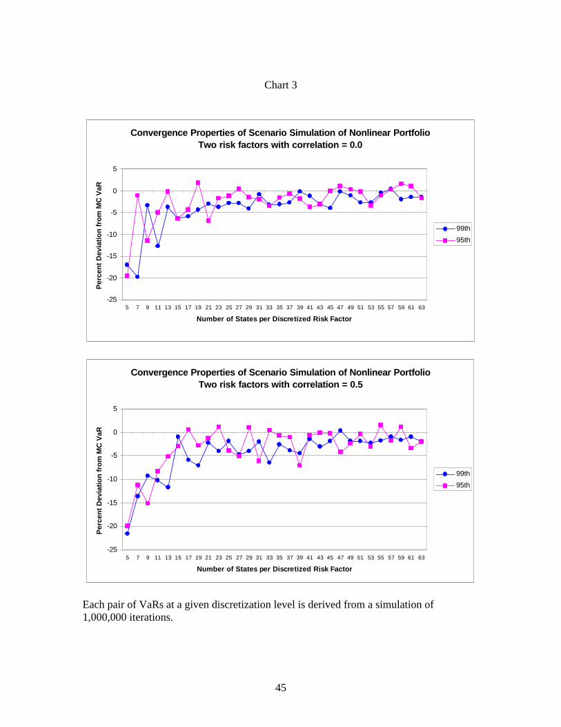
The pattern for the nonlinear portfolio shown in Chart 6 differs from the one in Chart
5 mainly in the substantial underestimate of the scenario simulation VaR in relation to the
corresponding Monte Carlo VaR. The sizable understatement diminishes only at
discretization levels—about 13 to 20 states per factor—that probably are impractical for
scenario simulation on large portfolios. As in the linear case, there also appears to be a
stronger tendency for the 99th percentile VaRs to underestimate the actual 99th percentile
VaR compared to the 95th percentile results.15
6. Conclusions The chief difficulty with standard Monte Carlo and principal component simulation in
VaR applications is the potentially intractable number of portfolio revaluations that must
be made in the course of computing VaR for very large portfolios. Jamshidian and Zhu
have suggested scenario simulation as a solution that permits the use of full revaluation.
15 Non-parametric 99 percent confidence intervals on the Monte Carlo benchmarks are:
Correlation 99% VaR 95% VaR 0.0 (-0.85%, 0.63%) (-0.64%, 0.50%) 0.5 (-0.98%, 0.67%) (-0.71%, 0.58%)

27
This paper has clarified the mechanics of computing VaR by scenario simulation and has
compared the VaR results from scenario simulation on several LIBOR-derivatives
portfolios with those from standard Monte Carlo and principal component simulation.
For the multicurrency interest rate derivatives portfolios examined in this paper,
the relative performance of scenario simulation was erratic. The outcomes for the
nonlinear test portfolios demonstrate that scenario simulation using low- and moderate-
dimensional discretizations can give “poor” estimates of VaR. Although the discrete
distributions used in scenario simulation converge to their continuous distributions,
convergence appears to be slow, with irregular oscillations that depend on portfolio
characteristics and the correlation structure of the risk factors. It would therefore be
prudent for any bank adopting this approach to test scenario-simulated VaR results
periodically against results from standard Monte Carlo or principal component
simulation.
The two-sided confidence intervals were computed using the method in Morokoff et al. (1998).

28
Appendix Standard Granger causality tests were run on “adjacent” maturity spot LIBOR tL and
swap rates tS to determine the degree of nonsynchroneity in the two data sources for the
LIBOR term structure. The spot LIBOR maturity was 1 year and the swap rate tenor was
2 years, the breakpoint in the market data used to estimate the forward LIBOR curve. The
following autoregression tests the null that coefficients 1 2 0pβ β β= = = =L , that is, the
swap rates do not Granger-cause spot LIBOR:
(A.1) 11 1
p p
t j t j j t jj j
L c L Sα β− −= =
= + +∑ ∑ .
Similarly, the null that spot LIBOR does not Granger-cause the swap rate is assessed
using
(A.2) 21 1
p p
t j t j j t jj j
S c S Lα β− −= =
= + +∑ ∑ .
These autoregressions are run on both daily and weekly interest rate data. The null is
tested based on the White heteroscedasticity-consistent covariance matrix estimator;
hence a chi-square rather than an F statistic is reported.
Granger Causality Tests Daily Weekly
Variable tested:
LIBOR
Swap Rate
LIBOR
Swap Rate
USD 2χ 22.5 300.19 7.95 29.97 p-value 0.001 0 0.242 0
DEM 2χ 7.08 244.39 10.23 11.86 p-value 0.31 0 0.115 0.065
CHF 2χ 8.17 273.36 13.35 18.2 p-value 0.226 0 0.038 0.006
GBP 2χ 13.39 312.78 10.53 14.6 p-value 0.037 0 0.104 0.024
29
The table shows the results for 6 lags in the autoregressions. Qualitatively similar results
were obtained for other values of p. The chi-square values overwhelmingly indicate that
swap rates Granger-cause spot LIBOR in the daily data, with weaker reverse feedback
from LIBOR to the swap rate for USD and GBP. Switching to a weekly periodicity
greatly reduces the magnitudes of the chi-square statistics for the swap rates, although
Granger-causation is still highly statistically significant for USD, CHF, and GBP.

30
References Derman, Emanuel. “Reflections on Fischer.” Journal of Portfolio Management, Special
Issue, 1996.
Dwyer, Jerry. “Quick and Portable Random Number Generators.” C/C++ Users Journal (June 1995), 33-44.
Engel, James and Marianne Gizycki. “Conservatism, Accuracy, and Efficiency: Comparing Value-at-Risk Models.” Working Paper 2, Australian Prudential Regulation Authority, March 1999.
Frye, Jon. “Principals of Risk: Finding Value-at-Risk Through Factor-Based Interest Rate Scenarios.” NationsBanc-CRT, April 1997.
Frye, Jon. “Monte Carlo by Day: Intraday Value-at-Risk Using Monte Carlo Simulation,” Risk, November 1998.
Hull, John. Options, Futures, and Other Derivative Securities. Englewood Cliffs, N.J.: Prentice Hall, 2000.
Hull, John and Alan White, “Value at Risk When Daily Changes in Market Variables are Not Normally Distributed.” Journal of Derivatives (Spring 1998), 9-19.
Jamshidian, Farshid. “Libor and Swap Market Models and Measures.” Finance and
Stochastics 1 (1997), 293-330.
Jamshidian, Farshid and Yu Zhu, “Scenario Simulation: Theory and Methodology.” Finance and Stochastics 1 (1997), 43-67.
Kreinin, Alexander, Leonid Merkoulovitch, Dan Rosen, and Michael Zerbs. “Principal Component Analysis in Quasi Monte Carlo Simulation.” Algo Research Quarterly, December 1998, 21-29.
Morokoff, William, Ron Lagnado, and Art Owen. “Tolerance for Risk.” Risk June 1998, 78-83.
Musiela, Marek, and Marek Rutkowski. Martingale Methods in Financial Modelling. New York: Springer-Verlag, 1997.
Overdahl, James A., Barry Schachter, and Ian Lang. “The Mechanics of Zero-Coupon Yield Curve Construction.” in Controlling & Managing Interest-Rate Risk, Anthony G. Cornyn, et al. eds. New York: New York Institute of Finance, 1997.
Picoult, Evan. “Calculating Value-at-Risk with Monte Carlo Simulation.” in Risk Management in Financial Institutions, Risk Publications, 1997.
Rebonato, Riccardo. Interest-Rate Option Models. Second Ed. New York: John Wiley & Sons, 1998.
Reimers, Mark and Michael Zerbs. “Dimension Reduction by Asset Blocks.” Algo Research Quarterly, December 1998, 43-57.
Singh, Manoj K. “Value at Risk Using Principal Components Analysis,” Journal of Portfolio Management (Fall 1997), 101-112.

31
Wang, Ti. “Learning Curve: Mathematical and Market-Generated Spikes in Forward Curves.” Derivatives Week, November 7, 1994.
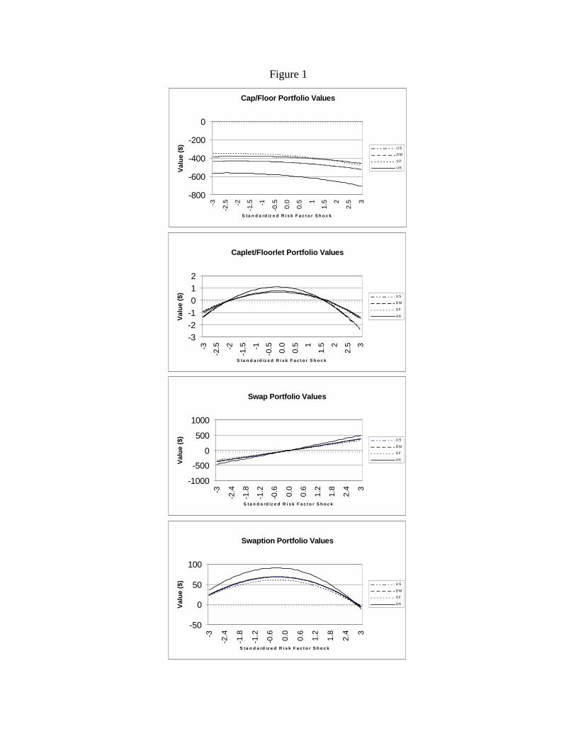
Figure 1
Cap/Floor Portfolio Values
-800
-600
-400
-200
0
-3
-2.5 -2
-1.5 -1
-0.5
0.0
0.5 1
1.5 2
2.5 3
S t a n d a rd iz e d R i s k F a c t o r S h o c k
Val
ue
($)
U S
D M
S F
U K
Caplet/Floorlet Portfolio Values
-3-2-1012
-3
-2.5 -2
-1.5 -1
-0.5 0.0
0.5 1
1.5 2
2.5 3
S t a n d a rd iz e d R i s k F a c t o r S h o c k
Val
ue
($)
U S
D M
S F
U K
Swap Portfolio Values
-1000
-500
0
500
1000
-3
-2.4
-1.8
-1.2
-0.6 0.0
0.6
1.2
1.8
2.4 3
S t a n d a rd iz e d R i s k F a c t o r S h o c k
Val
ue
($)
U S
D M
S F
U K
Swaption Portfolio Values
-50
0
50
100
-3
-2.4
-1.8
-1.2
-0.6 0.0
0.6
1.2
1.8
2.4 3
S t a n d a rd iz e d R i s k F a c t o r S h o c k
Val
ue
($)
U S
D M
S F
U K
33
Table 2 Correlation Matrix for 1994
Orange or dark shading denotes correlation coefficients ≥ 0 20. .
Table 3
Correlation Matrix for 1995
Orange or dark shading denotes correlation coefficients ≥ 0 20. .
USD DEM CHF GBP
PC1 PC2 PC3 PC1 PC2 PC3 PC1 PC2 PC3 PC1 PC2 PC3 DEM CHF GPB
PC1 1.0000 0.0000 0.0000
USD PC2 0.0000 1.0000 0.0000
PC3 0.0000 0.0000 1.0000
PC1 0.2433 -0.0357 0.1458 1.0000 0.0000 0.0000
DEM PC2 -0.2416 0.0137 0.0724 0.0000 1.0000 0.0000
PC3 0.1810 -0.0906 -0.1117 0.0000 0.0000 1.0000
PC1 0.2366 0.1240 0.2267 0.7006 -0.0345 -0.0837 1.0000 0.0000 0.0000
CHF PC2 -0.2309 0.0207 0.2085 -0.3727 0.3201 -0.0895 0.0000 1.0000 0.0000
PC3 0.0708 0.0886 -0.1887 0.0094 -0.5085 0.2588 0.0000 0.0000 1.0000
PC1 0.4194 -0.0908 -0.1216 0.5305 -0.3091 0.1053 0.4163 -0.4553 0.1207 1.0000 0.0000 0.0000
GBP PC2 -0.2337 0.0954 0.1328 -0.1965 0.4296 -0.1241 -0.1825 0.1844 -0.2631 0.0000 1.0000 0.0000
PC3 0.0438 -0.0724 -0.0660 -0.0469 0.0377 0.3783 -0.2672 -0.0510 -0.1307 0.0000 0.0000 1.0000
DEM 0.0314 -0.0725 0.0206 -0.1388 0.2672 0.1691 -0.0511 0.1776 -0.1031 -0.1736 0.0332 0.0499 1.0000 0.9239 0.7634
CHF 0.1150 -0.0036 0.0726 -0.1197 0.2388 0.1932 -0.0426 0.1977 -0.1046 -0.1348 -0.0313 0.0040 0.9239 1.0000 0.7563
GPB 0.1943 -0.1161 0.0324 -0.0663 0.2006 0.2157 0.1110 0.3074 -0.1020 -0.0765 -0.1612 -0.0256 0.7634 0.7563 1.0000
USD DEM CHF GBP
PC1 PC2 PC3 PC1 PC2 PC3 PC1 PC2 PC3 PC1 PC2 PC3 DEM CHF GPB
PC1 1.0000 0.0000 0.0000
USD PC2 0.0000 1.0000 0.0000
PC3 0.0000 0.0000 1.0000
PC1 0.2977 0.2511 0.1268 1.0000 0.0000 0.0000
DEM PC2 -0.4841 0.0152 0.0831 0.0000 1.0000 0.0000
PC3 0.0688 0.0644 0.1454 0.0000 0.0000 1.0000
PC1 0.0872 0.1761 0.0553 0.5861 0.1963 -0.0588 1.0000 0.0000 0.0000
CHF PC2 -0.3354 -0.0020 -0.0035 -0.3962 0.5769 0.0562 0.0000 1.0000 0.0000
PC3 -0.0124 0.1440 0.0728 -0.0835 0.0840 0.0833 0.0000 0.0000 1.0000
PC1 0.4785 0.1449 0.0788 0.4872 -0.5455 0.0555 0.1444 -0.4044 -0.1173 1.0000 0.0000 0.0000
GBP PC2 -0.0648 0.1061 0.0908 0.0392 0.4639 0.1713 0.1627 0.2105 0.1186 0.0000 1.0000 0.0000
PC3 0.2025 0.1449 0.0325 0.2762 -0.0923 0.2700 -0.0187 -0.3401 0.1400 0.0000 0.0000 1.0000
DEM -0.1973 0.0410 -0.1658 0.1313 0.2656 -0.3284 0.4029 0.0970 0.0320 -0.2285 0.0287 -0.1690 1.0000 0.9480 0.7821
CHF -0.1110 0.0157 -0.0788 0.2146 0.1769 -0.2842 0.4599 -0.0012 -0.0406 -0.1278 0.0159 -0.1737 0.9480 1.0000 0.7399
GPB -0.2338 -0.1090 -0.2077 0.0544 0.2291 -0.1911 0.2107 0.2654 -0.0347 -0.1588 -0.1547 -0.1733 0.7821 0.7399 1.0000
34
Table 4 Correlation Matrix for 1996
USD DEM CHF GBP
PC1 PC2 PC3 PC1 PC2 PC3 PC1 PC2 PC3 PC1 PC2 PC3 DEM CHF GPB
PC1 1.0000 0.0000 0.0000
USD PC2 0.0000 1.0000 0.0000
PC3 0.0000 0.0000 1.0000
PC1 0.1835 0.1280 -0.0053 1.0000 0.0000 0.0000
DEM PC2 -0.3702 -0.0632 -0.0320 0.0000 1.0000 0.0000
PC3 0.1874 -0.0636 -0.0646 0.0000 0.0000 1.0000
PC1 0.1885 0.0743 0.0426 0.2008 -0.5270 0.0857 1.0000 0.0000 0.0000
CHF PC2 0.0028 0.0696 -0.0599 0.2304 0.1536 -0.3383 0.0000 1.0000 0.0000
PC3 -0.1078 -0.0376 -0.2738 -0.2031 0.2122 0.1032 0.0000 0.0000 1.0000
PC1 0.2976 -0.0748 -0.1314 0.0387 -0.3411 0.2986 0.1992 -0.1477 -0.2207 1.0000 0.0000 0.0000
GBP PC2 -0.3897 0.1677 -0.1583 0.0812 0.2347 -0.3899 -0.2045 0.2512 0.0176 0.0000 1.0000 0.0000
PC3 -0.0415 -0.1877 0.0432 -0.1639 0.1666 -0.0255 0.1491 -0.2525 0.1632 0.0000 0.0000 1.0000
DEM -0.1648 0.0493 -0.0433 -0.0331 0.3982 -0.0179 -0.0414 0.1605 0.2381 -0.3227 0.1500 0.0664 1.0000 0.9082 0.5467
CHF -0.1446 0.1074 -0.0079 -0.0147 0.2580 0.0678 0.1123 0.0395 0.2135 -0.2431 0.1968 0.0786 0.9082 1.0000 0.3939
GPB 0.0158 -0.1582 0.0315 -0.1182 0.4321 0.1001 -0.2499 0.2005 0.1301 -0.3019 -0.1001 -0.1275 0.5467 0.3939 1.0000
Orange or dark shading denotes correlation coefficients ≥ 0 20. .
Table 5
Correlation Matrix for 1997
Orange or dark shading denotes correlation coefficients ≥ 0 20. .
USD DEM CHF GBP
PC1 PC2 PC3 PC1 PC2 PC3 PC1 PC2 PC3 PC1 PC2 PC3 DEM CHF GPB
PC1 1.0000 0.0000 0.0000
USD PC2 0.0000 1.0000 0.0000
PC3 0.0000 0.0000 1.0000
PC1 0.2038 0.2331 -0.2225 1.0000 0.0000 0.0000
DEM PC2 -0.4812 -0.0061 -0.0237 0.0000 1.0000 0.0000
PC3 0.3724 -0.2849 0.1437 0.0000 0.0000 1.0000
PC1 -0.0521 0.2049 -0.0963 0.1181 -0.3524 -0.3831 1.0000 0.0000 0.0000
CHF PC2 -0.2835 -0.1072 0.2664 -0.3935 0.2929 -0.2211 0.0000 1.0000 0.0000
PC3 0.1981 -0.0974 -0.1996 0.0757 -0.0847 -0.0414 0.0000 0.0000 1.0000
PC1 0.3952 0.1504 0.0119 0.1930 -0.4372 0.3689 0.0344 -0.2904 0.1653 1.0000 0.0000 0.0000
GBP PC2 -0.4174 0.3071 -0.0839 -0.1467 0.2206 -0.3406 -0.0340 0.1567 0.1784 0.0000 1.0000 0.0000
PC3 -0.1641 0.1786 0.0832 0.1539 -0.1095 -0.2622 0.1541 0.0241 -0.3206 0.0000 0.0000 1.0000
DEM -0.0067 0.1331 -0.2346 0.0235 0.0594 -0.1519 0.0677 -0.0728 0.0815 -0.1494 -0.0170 0.0382 1.0000 0.8619 0.5048
CHF 0.0445 0.0899 -0.2982 0.0595 0.0594 -0.1570 0.1325 -0.1244 0.0245 -0.2129 -0.0648 0.0383 0.8619 1.0000 0.5042
GPB 0.0636 0.0025 0.0284 0.1569 -0.1351 -0.1548 0.2061 -0.1543 0.0300 -0.1859 -0.2212 0.2953 0.5048 0.5042 1.0000
35
Table 6 Correlation Matrix for 1998
USD DEM CHF GBP
PC1 PC2 PC3 PC1 PC2 PC3 PC1 PC2 PC3 PC1 PC2 PC3 DEM CHF GPB
PC1 1.0000 0.0000 0.0000
USD PC2 0.0000 1.0000 0.0000
PC3 0.0000 0.0000 1.0000
PC1 0.5895 0.1920 0.1399 1.0000 0.0000 0.0000
DEM PC2 -0.1843 0.3053 -0.1411 0.0000 1.0000 0.0000
PC3 -0.0164 0.1013 0.4459 0.0000 0.0000 1.0000
PC1 0.2457 0.2168 -0.3287 0.2157 0.1724 -0.3276 1.0000 0.0000 0.0000
CHF PC2 -0.4962 0.1380 -0.3000 -0.5829 0.2149 0.1660 0.0000 1.0000 0.0000
PC3 -0.0526 -0.3017 0.2418 -0.0585 -0.2248 -0.0174 0.0000 0.0000 1.0000
PC1 0.3325 0.0345 0.2870 0.4608 -0.3084 0.1082 0.0504 -0.4726 0.1368 1.0000 0.0000 0.0000
GBP PC2 0.0275 0.2709 -0.1490 -0.0509 0.2179 -0.0809 0.0849 0.1430 0.0367 0.0000 1.0000 0.0000
PC3 -0.0440 -0.1809 0.3284 -0.0185 -0.1246 0.1316 -0.1899 -0.1496 0.0957 0.0000 0.0000 1.0000
DEM 0.2576 0.0872 -0.3963 0.1789 -0.0970 0.0143 0.2737 0.0900 -0.3002 0.2587 0.0303 -0.1092 1.0000 0.9109 0.5094
CHF 0.2706 0.0921 -0.4253 0.2371 -0.0515 -0.1046 0.4369 -0.0251 -0.2704 0.3278 -0.0036 -0.1872 0.9109 1.0000 0.3912
GPB 0.1794 -0.0708 -0.2995 0.0843 -0.0901 -0.1089 0.1925 0.1464 -0.1175 -0.2163 0.0882 -0.0387 0.5094 0.3912 1.0000
Orange or dark shading denotes correlation coefficients ≥ 0 20. .
36
Chart 1
PC/MC denotes the percentage deviation of the principal components VaR from the Monte Carlo VaR; SS7/PC denotes the 7 5 3 3× × × scenario simulation VaR relative to principal components VaR; SS11/PC denotes the 11 7 5 5× × × scenario simulation VaR relative to principal components VaR.
Comparison of 99th Percentile VaRs: 1994
-15.0-10.0-5.00.05.0
10.015.0
Caps Caplets Swaps Swaptions
Per
cen
t D
evia
tio
nPC/MC
SS7/PC
SS11/PC
Comparison of 99th Percentile VaRs: 1995
-25.0-20.0-15.0-10.0-5.00.05.0
Caps Caplets Swaps Swaptions
Per
cen
t D
evia
tio
n
PC/MC
SS7/PC
SS11/PC
Comparison of 99th Percentile VaRs: 1996
-15.0
-10.0
-5.0
0.0
5.0
Caps Caplets Swaps Swaptions
Per
cen
t D
evia
tio
n
PC/MC
SS7/PC
SS11/PC

37
Chart 1, continued
PC/MC denotes the percentage deviation of the principal components VaR from the Monte Carlo VaR; SS7/PC denotes the 7 5 3 3× × × scenario simulation VaR relative to principal components VaR; SS11/PC denotes the 11 7 5 5× × × scenario simulation VaR relative to principal components VaR.
Comparison of 99th Percentile VaRs: 1997
-20.0-15.0-10.0-5.00.05.0
10.015.0
Caps Caplets Swaps Swaptions
PC/MC
SS7/PC
SS11/PC
Comparison of 99th Percentile VaRs: 1998
-20.0-15.0-10.0-5.00.05.0
10.015.020.0
Caps Caplets Swaps Swaptions
PC/MC
SS7/PC
SS11/PC

38
Table 7
Four-Currency Interest Rate Derivate Portfolios
1994 Caps/Floors Caplets/Floorlets Swaps Swaptions 99th 95th 99th 95th 99th 95th 99th 95th
PC/MC -3.90 -1.28 -2.89 -1.35 1.52 -1.06 -3.95 -3.12SS7/PC -5.82 -3.93 -10.29 -5.86 -6.08 -2.24 -10.65 -5.12SS11/PC 9.14 15.21 -6.78 -4.19 -3.33 -0.19 -8.25 -8.35 1995 Caps/Floors Caplets/Floorlets Swaps Swaptions
99th 95th 99th 95th 99th 95th 99th 95thPC/MC -3.99 -5.09 1.22 -2.18 0.44 1.02 -4.45 -3.82SS7/PC -21.88 -17.74 -12.35 -4.77 -6.18 -3.65 -11.17 -6.48SS11/PC 2.09 13.47 -8.23 -3.76 -2.40 -0.54 -7.98 -9.87 1996 Caps/Floors Caplets/Floorlets Swaps Swaptions
99th 95th 99th 95th 99th 95th 99th 95thPC/MC -0.09 -0.99 -8.14 -9.52 -1.52 -4.30 -5.92 -4.28SS7/PC -11.11 -7.49 -7.26 -5.29 -4.62 -1.37 -12.71 -7.90SS11/PC 1.13 7.24 -4.69 -4.84 -1.17 0.91 -9.27 -8.67 1997 Caps/Floors Caplets/Floorlets Swaps Swaptions
99th 95th 99th 95th 99th 95th 99th 95thPC/MC -2.00 -5.75 0.94 -4.24 -7.56 -1.95 -1.32 -6.21SS7/PC -9.30 -3.56 -11.06 -6.19 -3.44 -3.71 -16.83 -8.56SS11/PC 10.48 22.80 -7.56 -4.61 -0.98 -1.46 -12.76 -10.49 1998 Caps/Floors Caplets/Floorlets Swaps Swaptions
99th 95th 99th 95th 99th 95th 99th 95thPC/MC 0.67 -1.62 -2.02 -2.57 -0.17 -2.83 -5.76 -4.11SS7/PC -2.93 0.66 -6.66 -3.75 -7.06 -2.61 -14.40 -8.32SS11/PC 15.74 23.78 -4.87 -2.97 -4.01 -0.20 -10.82 -10.19
PC/MC is the percentage deviation of the principal component VaR from the Monte Carlo VaR. SS7/PC is the percentage deviation of the 7 5 3 3× × × scenario simulation VaR from the principal component VaR. SS11/PC is the percentage deviation of the 11 7 5 5× × × scenario simulation VaR from the principal component VaR.

39
Table 8 Detailed Results
1994: Caps/Floors
Monte Carlo PC4 7x5x3x3 11x7x5x5
99th 95th 99th 95th 99th 95th 99th 95th
VaR 159.153 111.127 152.946 109.700 144.040 105.383 166.926 126.387
Std Dev. 8.127 3.466 9.734 3.325 1.970 1.089 2.087 0.787
Std Error 1.817 0.775 2.177 0.743 0.440 0.243 0.467 0.176
1994: Caplets/Floorlets
Monte Carlo PC4 7x5x3x3 11x7x5x5
99th 95th 99th 95th 99th 95th 99th 95th
VaR 2.674 1.437 2.597 1.418 2.330 1.334 2.421 1.358
Std Dev. 0.227 0.081 0.225 0.079 0.057 0.022 0.058 0.028
Std Error 0.051 0.018 0.050 0.018 0.013 0.005 0.013 0.006
1994: Swaps
Monte Carlo PC4 7x5x3x3 11x7x5x5
99th 95th 99th 95th 99th 95th 99th 95th
VaR 940.829 648.902 955.140 642.013 897.066 627.647 923.356 640.762
Std Dev. 59.107 23.946 50.360 24.845 13.049 8.117 13.351 7.966
Std Error 13.217 5.355 11.261 5.556 2.918 1.815 2.985 1.781
1994: Swaptions
Monte Carlo PC4 7x5x3x3 11x7x5x5
99th 95th 99th 95th 99th 95th 99th 95th
VaR 130.812 65.544 125.649 63.502 112.269 60.251 115.281 58.198
Std Dev. 10.996 4.782 12.274 4.701 3.219 1.445 3.010 1.009
Std Error 2.459 1.069 2.744 1.051 0.720 0.323 0.673 0.226
Results reported in dollars. The standard error is for the VaR at a given percentile, computed based on 20 runs of 1,000 iterations each for Monte Carlo and principal component VaR and 10,000 iterations for scenario simulation.

40
Table 8, continued Detailed Results
1995: Caps/Floors
Monte Carlo PC4 7x5x3x3 11x7x5x5
99th 95th 99th 95th 99th 95th 99th 95th
VaR 73.824 52.779 70.880 50.091 55.374 41.205 72.359 56.837
Std Dev. 4.667 1.910 3.777 2.125 0.814 0.379 0.845 0.361
Std Error 1.044 0.427 0.844 0.475 0.182 0.085 0.189 0.081
1995: Caplets/Floorlets
Monte Carlo PC4 7x5x3x3 11x7x5x5
99th 95th 99th 95th 99th 95th 99th 95th
VaR 1.896 1.013 1.919 0.991 1.682 0.943 1.761 0.954
Std Dev. 0.275 0.048 0.205 0.105 0.035 0.019 0.036 0.019
Std Error 0.061 0.011 0.046 0.023 0.008 0.004 0.008 0.004
1995: Swaps
Monte Carlo PC4 7x5x3x3 11x7x5x5
99th 95th 99th 95th 99th 95th 99th 95th
VaR 491.033 333.107 493.177 336.520 462.707 324.244 481.345 334.692
Std Dev. 19.749 15.063 29.659 16.037 8.865 4.157 7.262 5.181
Std Error 4.416 3.368 6.632 3.586 1.982 0.930 1.624 1.159
1995: Swaptions
Monte Carlo PC4 7x5x3x3 11x7x5x5
99th 95th 99th 95th 99th 95th 99th 95th
VaR 59.544 30.463 56.895 29.298 50.539 27.401 52.357 26.408
Std Dev. 8.161 2.243 4.390 1.780 1.418 0.429 1.415 0.549
Std Error 1.825 0.502 0.982 0.398 0.317 0.096 0.316 0.123
Results reported in dollars. The standard error is for the VaR at a given percentile, computed based on 20 runs of 1,000 iterations each for Monte Carlo and principal component VaR and 10,000 iterations for scenario simulation.

41
Table 8, continued Detailed Results
1996: Caps/Floors
Monte Carlo PC4 7x5x3x3 11x7x5x5
99th 95th 99th 95th 99th 95th 99th 95th
VaR 81.816 58.560 81.744 57.980 72.660 53.638 82.666 62.176
Std Dev. 3.240 1.912 3.975 1.953 0.965 0.389 1.468 0.531
Std Error 0.724 0.428 0.889 0.437 0.216 0.087 0.328 0.119
1996: Caplets/Floorlets
Monte Carlo PC4 7x5x3x3 11x7x5x5
99th 95th 99th 95th 99th 95th 99th 95th
VaR 2.070 1.096 1.901 0.992 1.763 0.939 1.812 0.944
Std Dev. 0.157 0.088 0.244 0.050 0.045 0.019 0.048 0.018
Std Error 0.035 0.020 0.054 0.011 0.010 0.004 0.011 0.004
1996: Swaps
Monte Carlo PC4 7x5x3x3 11x7x5x5
99th 95th 99th 95th 99th 95th 99th 95th
VaR 479.380 333.362 472.100 319.029 450.281 314.660 466.572 321.944
Std Dev. 24.958 12.000 29.377 12.295 5.680 3.803 5.553 3.963
Std Error 5.581 2.683 6.569 2.749 1.270 0.850 1.242 0.886
1996: Swaptions
Monte Carlo PC4 7x5x3x3 11x7x5x5
99th 95th 99th 95th 99th 95th 99th 95th
VaR 59.738 30.539 56.200 29.233 49.059 26.924 50.993 26.698
Std Dev. 7.046 2.134 5.280 2.087 1.149 0.413 1.309 0.609
Std Error 1.575 0.477 1.181 0.467 0.257 0.092 0.293 0.136
Results reported in dollars. The standard error is for the VaR at a given percentile, computed based on 20 runs of 1,000 iterations each for Monte Carlo and principal component VaR and 10,000 iterations for scenario simulation.

42
Table 8, continued Detailed Results
1997: Caps/Floors
Monte Carlo PC4 7x5x3x3 11x7x5x5
99th 95th 99th 95th 99th 95th 99th 95th
VaR 74.880 53.855 73.385 50.759 66.557 48.951 81.074 62.333
Std Dev. 4.696 2.266 4.007 2.293 0.998 0.405 1.111 0.458
Std Error 1.050 0.507 0.896 0.513 0.223 0.091 0.249 0.102
1997: Caplets/Floorlets
Monte Carlo PC4 7x5x3x3 11x7x5x5
99th 95th 99th 95th 99th 95th 99th 95th
VaR 2.259 1.189 2.281 1.139 2.028 1.068 2.108 1.086
Std Dev. 0.218 0.076 0.232 0.063 0.048 0.027 0.084 0.025
Std Error 0.049 0.017 0.052 0.014 0.011 0.006 0.019 0.006
1997: Swaps
Monte Carlo PC4 7x5x3x3 11x7x5x5
99th 95th 99th 95th 99th 95th 99th 95th
VaR 558.799 368.531 516.547 361.331 498.765 347.917 511.459 356.071
Std Dev. 19.522 14.999 30.331 19.930 6.500 5.030 9.029 3.694
Std Error 4.365 3.354 6.782 4.456 1.453 1.125 2.019 0.826
1997: Swaptions
Monte Carlo PC4 7x5x3x3 11x7x5x5
99th 95th 99th 95th 99th 95th 99th 95th
VaR 68.428 35.532 67.523 33.326 56.162 30.472 58.906 29.829
Std Dev. 4.922 2.109 6.603 2.784 1.571 0.574 1.485 0.708
Std Error 1.101 0.472 1.476 0.622 0.351 0.128 0.332 0.158
Results reported in dollars. The standard error is for the VaR at a given percentile, computed based on 20 runs of 1,000 iterations each for Monte Carlo and principal component VaR and 10,000 iterations for scenario simulation.
43
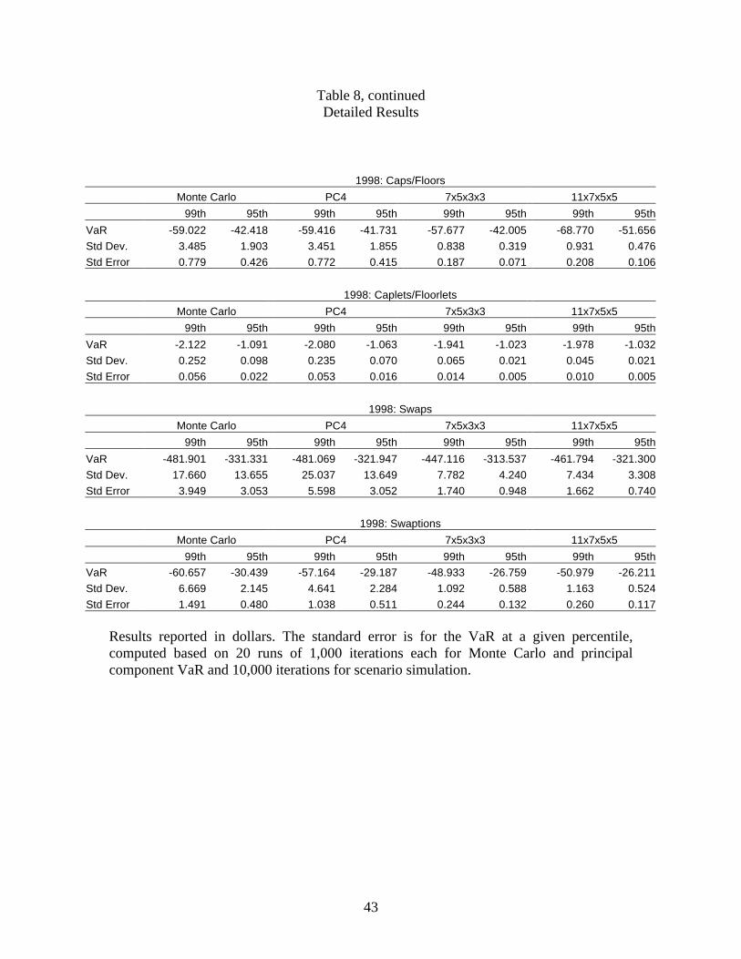
Table 8, continued Detailed Results
1998: Caps/Floors
Monte Carlo PC4 7x5x3x3 11x7x5x5
99th 95th 99th 95th 99th 95th 99th 95th
VaR -59.022 -42.418 -59.416 -41.731 -57.677 -42.005 -68.770 -51.656
Std Dev. 3.485 1.903 3.451 1.855 0.838 0.319 0.931 0.476
Std Error 0.779 0.426 0.772 0.415 0.187 0.071 0.208 0.106
1998: Caplets/Floorlets
Monte Carlo PC4 7x5x3x3 11x7x5x5
99th 95th 99th 95th 99th 95th 99th 95th
VaR -2.122 -1.091 -2.080 -1.063 -1.941 -1.023 -1.978 -1.032
Std Dev. 0.252 0.098 0.235 0.070 0.065 0.021 0.045 0.021
Std Error 0.056 0.022 0.053 0.016 0.014 0.005 0.010 0.005
1998: Swaps
Monte Carlo PC4 7x5x3x3 11x7x5x5
99th 95th 99th 95th 99th 95th 99th 95th
VaR -481.901 -331.331 -481.069 -321.947 -447.116 -313.537 -461.794 -321.300
Std Dev. 17.660 13.655 25.037 13.649 7.782 4.240 7.434 3.308
Std Error 3.949 3.053 5.598 3.052 1.740 0.948 1.662 0.740
1998: Swaptions
Monte Carlo PC4 7x5x3x3 11x7x5x5
99th 95th 99th 95th 99th 95th 99th 95th
VaR -60.657 -30.439 -57.164 -29.187 -48.933 -26.759 -50.979 -26.211
Std Dev. 6.669 2.145 4.641 2.284 1.092 0.588 1.163 0.524
Std Error 1.491 0.480 1.038 0.511 0.244 0.132 0.260 0.117
Results reported in dollars. The standard error is for the VaR at a given percentile, computed based on 20 runs of 1,000 iterations each for Monte Carlo and principal component VaR and 10,000 iterations for scenario simulation.

44
Chart 2
Each pair of VaRs at a given discretization level is derived from a simulation of 1,000,000 iterations.
Convergence Properties of Scenario Simulation of Linear Portfolio Two risk factors with correlation = 0.0
-20
-15
-10
-5
0
5
10
5 7 9 11 13 15 17 19 21 23 25 27 29 31 33 35 37 39 41 43 45 47 49 51 53 55 57 59 61 63
Number of States per Discretized Risk Factor
Per
cen
t D
evia
tio
n f
rom
VC
VaR
99th
95th
Convergence Properties of Scenario Simulation of Linear PortfolioTwo risk factors with correlation = 0.5
-20
-15
-10
-5
0
5
10
5 7 9 11 13 15 17 19 21 23 25 27 29 31 33 35 37 39 41 43 45 47 49 51 53 55 57 59 61 63
Number of States per Discretized Risk Factor
Per
cen
t D
evia
tio
n f
rom
VC
VaR
99th
95th
45
Chart 3
Each pair of VaRs at a given discretization level is derived from a simulation of 1,000,000 iterations.
Convergence Properties of Scenario Simulation of Nonlinear PortfolioTwo risk factors with correlation = 0.5
-25
-20
-15
-10
-5
0
5
5 7 9 11 13 15 17 19 21 23 25 27 29 31 33 35 37 39 41 43 45 47 49 51 53 55 57 59 61 63
Number of States per Discretized Risk Factor
Per
cen
t D
evia
tio
n f
rom
MC
VaR
99th
95th
Convergence Properties of Scenario Simulation of Nonlinear PortfolioTwo risk factors with correlation = 0.0
-25
-20
-15
-10
-5
0
5
5 7 9 11 13 15 17 19 21 23 25 27 29 31 33 35 37 39 41 43 45 47 49 51 53 55 57 59 61 63
Number of States per Discretized Risk Factor
Per
cen
t D
evia
tio
n f
rom
MC
VaR
99th
95th