An Empirical Evaluation of Bayesian Networks Derivedfrom Fault TreesShane Strasser and John SheppardDepartment of Computer Science

Montana State UniversityBozeman, MT 59717

{shane.strasser, john.sheppard}@cs.montana.edu

Abstract—Fault Isolation Manuals (FIMs) are derived from atype of decision tree and play an important role in maintenancetroubleshooting of large systems. However, there are somedrawbacks to using decision trees for maintenance, such asrequiring a static order of tests to reach a conclusion. Onemethod to overcome these limitations is by converting FIMs toBayesian networks. However, it has been shown that Bayesiannetworks derived from FIMs will not contain the entire set offault and alarm relationships present in the system from whichthe FIM was developed. In this paper we analyze Bayesiannetworks that have been derived from FIMs and report onseveral measurements, such as accuracy, relative probability oftarget diagnoses, diagnosis rank, and KL-divergence. Based onour results, we found that even with incomplete information,the Bayesian networks derived from the FIMs were still able toperform reasonably well.

TABLE OF CONTENTS

1 INTRODUCTION . . . . . . . . . . . . . . . . . . . . . . . . . . . . . . . . . . 12 DIAGNOSTIC MODELS . . . . . . . . . . . . . . . . . . . . . . . . . . . 23 CONVERTING FIMS . . . . . . . . . . . . . . . . . . . . . . . . . . . . . 54 EXPERIMENTS . . . . . . . . . . . . . . . . . . . . . . . . . . . . . . . . . . . 65 RESULTS . . . . . . . . . . . . . . . . . . . . . . . . . . . . . . . . . . . . . . . . . 86 CONCLUSIONS . . . . . . . . . . . . . . . . . . . . . . . . . . . . . . . . . . . 117 SUMMARY . . . . . . . . . . . . . . . . . . . . . . . . . . . . . . . . . . . . . . . 12

ACKNOWLEDGMENTS . . . . . . . . . . . . . . . . . . . . . . . . . . . 12REFERENCES . . . . . . . . . . . . . . . . . . . . . . . . . . . . . . . . . . . . 12BIOGRAPHY . . . . . . . . . . . . . . . . . . . . . . . . . . . . . . . . . . . . . 13

1. INTRODUCTIONPerforming fault diagnosis is an extremely difficult problem[1]. Given a complex system and a set of tests or alarmoutcomes, the user wants to determine the most likely faultycomponent. One diagnostic tool that is often utilized isthe Fault Isolation Manual (FIM). FIMs are derived froma type of decision tree and allow users to isolate faults atthe lowest component level [2]. The user performs the testcorresponding to the root of the tree and follows the branchbased on the test outcome to the next test specified in the FIM.This process is repeated until the user reaches a leaf in the treecorresponding to the diagnosed fault.

However, there are some drawbacks to using decision treesfor maintenance, such as requiring a static order of tests toreach a conclusion. For example, suppose the maintaineronly has access to a subset of the test resources required by aFIM (e.g., the oscilloscope is broken). Using a static FIM,determining which faults are diagnosed based on only the

978-1-4673-1813-6/13/$31.00 c©2013 IEEE.1 IEEEAC Paper #2714, Version 03, Updated 29/01/2013 .

available tests can lead a difficult problem, especially if testsrequiring unavailable resources occur higher in the tree. Oneway to overcome this limitation is to convert the FIM to analternate type of model that allows for dynamically orderedtest sequences, such as D-Matrices (i.e., the set of all therelationships between a set of alarms and faults) or Bayesiannetworks.

In this paper we look at converting FIMs to Bayesian net-works. In addition to allowing for a dynamic ordering oftests, converting static FIMs to Bayesian networks has severalother advantages. The first is that it allows for probabilisticreasoning over the system. Another is that certain processes,such as diagnostic model maturation, are more naturallysuited for Bayesian networks. While there are algorithmsthat do allow for the incremental updating of decision trees,these algorithms assume that one has access to all of the dataused to generate the trees, which will not always be the case,especially when using FIMs generated by domain experts [3].

Bayesian networks have been used extensively for fault diag-nosis. Traditionally, there are two ways for building Bayesiannetworks; the first is to build the network from data usinga learning algorithm. The other is to build the network byhand with the aid of a systems expert and manually definethe structure and parameters of each random variable [4].Additionally, one can use some combination of these twomethods: First start with a network built by a domain expertand then use a learning algorithm to refine the Bayesiannetwork [5].

There has also been work in deriving Bayesian networks fromother models. Starting with a fault tree used in fault treeanalysis, one can derive a Bayesian network representing thevarious logic gates in the fault tree [6], [7]. This work waslater extended to allow dynamic fault trees to be convertedinto Bayesian networks by utilizing dynamic Bayesian net-works [8]. However these fault trees are not decision trees.Dependency networks are another type of model that has beenused to aid in constructing Bayesian networks. In [9], theauthors first constructed dependency networks because suchnetworks are often easier to learn than Bayesian networks.They then used an oracle to construct the Bayesian networksfrom the dependency networks. Our work is similar in that weare using a model containing relationships between tests andfaults (i.e., dependencies) to construct Bayesian networks,except that in our case, we the dependencies are specifiedusing D-Matrices derived from fault trees. In addition, this isthe first paper to analyze the performance of these Bayesiannetworks derived from FIMs.

Given a FIM, one can construct a D-Matrix representing thefault and test relationships in the FIM. From the D-Matrixderived from the FIM, one can then construct a bipartiteBayesian network, similar to the Bayesian network presented

1

in QMR-DT [10], [11]. However, it has been shown thatit is not feasible to derive a full D-Matrix from a FIM[2]; therefore, any Bayesian network derived from such aD-Matrix will not represent the entire set of relationshipsbetween faults and tests in the system.

Despite this limitation, we hypothesize that bipartiteBayesian networks derived from FIMs can still performreasonably well. To test this hypothesis, we derive severalFIMs, each from multiple D-Matrices. Using these FIMs, wethen generate the resulting Bayesian network by convertingthe FIM to a partial D-Matrix and then the D-Matrix toa Bayesian network. Additionally, we create a Bayesiannetwork from the original D-Matrix, treating that networkas “ground truth.” We then evaluate the Bayesian networkscreated from the FIMs by comparing them to the Bayesiannetwork derived from the original D-Matrix and report onseveral measurements, such as accuracy, relative probabilityof target diagnoses, diagnosis rank, and KL-divergence. Inour results, we found that even with the incomplete informa-tion derived from the FIM, fairly high diagnostic accuracyresults when using the corresponding Bayesian networks.

The rest of the paper is organized as follows. Section 2gives a formal definition of D-Matrices, FIMs, and Bayesiannetworks while Section 3 gives a formal algorithm on howto derive Bayesian networks from FIMs. The experimentsin the paper are presented in Section 4 with the results inSection 5. Finally, analyses of the results are in Section 6and conclusions in Section 7.

2. DIAGNOSTIC MODELSThere are several ways to perform fault diagnosis [1]. Someof the most common diagnostic algorithms are rule-basedalgorithms, such as those in [12]. Fault dictionaries are an-other diagnostic method that have successfully been appliedto various systems [13]. Fault trees have also been mergedwith rule-oriented reasoning, which allows for locating andidentifying failures [14]. As we have already discussed, FaultIsolation Manuals (FIMs) are a type of decision tree or faulttree that provide another means to perform fault diagnosis.Model-based methods, which compare observations from thesystem with those expected from a model, provide anothercommon set of approaches to performing system-level di-agnosis [15]. Another diagnostic algorithm that has beenextensively used for fault diagnostics and prognostics areBayesian networks, which allow for a compact representationof probability distributions [10], [16]. Diagnostic modelsand Bayesian networks can be represented as D-Matrices [1].D-Matrices are matrix representations of the relationshipsbetween faults and tests (or alarms) in a diagnostic model [1].The rest of this section gives a more detailed explanation ofD-Matrices, FIMs, and Bayesian networks.

D-Matrices

One way diagnostic models can be represented is with D-Matrices. A D-Matrix relate the faults and the tests monitoror observe those faults. We can formally define it as thefollowing: Let F represent a set of faults and T represent a setof tests. Assume each Fi ∈ F is a Boolean variable such thateval(Fi) ∈ {0, 1} and each Tj ∈ T is also a Boolean variablesuch that eval(Fi,Tj) ∈ {0, 1}. We define eval(Fj , Tj) tothen be the following:

eval(Fi,Tj) =

{1 if Tj detects Fi

0 otherwise

Figure 1: A logic diagram for the Simple Model fromSimpson and Sheppard [1].

Table 1: The D-Matrix for Figure 1.

TINT1 T01 T02 T03 T04 T05 T06 T07FINT1 1 1 1 1 1 1 1 1

F01 0 1 1 1 1 1 1 1F02 0 0 1 1 0 0 0 1F03 0 0 0 1 1 1 1 1F04 0 0 0 1 0 0 0 1F05 0 0 0 0 0 0 0 1F06 0 0 0 0 0 1 0 1F07 0 0 0 1 1 1 1 1F08 0 0 0 0 0 0 0 1F09 0 0 0 1 1 1 1 1NF 0 0 0 0 0 0 0 0

Then a diagnostic signature is defined to be the vector

Fi =[eval(Fi,T1), . . . , eval(Fi,T|T|)

]A D-Matrix is then defined to be the set of diagnostic sig-natures Fi for all Fi ∈ F [17]. Rows represent faults andcolumns represent tests. The ith column corresponds to testTi in the diagnostic model. Table 1 shows an example D-Matrix representing the logic diagram of the diagnostic modelin Figure 1. In the Simple Model there are 7 tests, 10 faultsincluding no fault found (which is not shown in the logicdiagram), and 1 testable input.

Fault Isolation Manuals

Fault Isolation Manuals (FIMs) provide diagnostic strategiesusing structured sequences of tests to diagnose the root causeof fault codes that are reported by on-board diagnostic sys-tems [1]. At each step, a test is performed and depending onthe test outcome (pass or fail), the FIM then gives the nexttest that should be performed. This process is repeated until asingle fault or ambiguity group is diagnosed as the cause forthe fault code.

FIMs are often represented as fault trees, which is a particularkind of decision tree.2 A decision tree is a tree data structure

2The term “fault tree” has also been used to define a tree-like structure in

2

Figure 2: An example FIM derived from the D-Matrix inTable 1.

composed of internal decision nodes and terminal leaves [18].At each decision node, there is a test function with a set ofoutcomes. Given an input at each decision node, the testfunction is used and a branch from the decision node is takencorresponding to the outcome of the test function. To classifya single data instance, the process begins at the root node andthen evaluates the attributes by applying the test to the datapoint being classified. The tree is then traversed along theedges to the next appropriate test until a leaf node is reached.The leaf node’s label is then assigned to the current instancethat is being classified.

In machine learning, decision trees are often built using in-formation gain or the Gini index [18]. Given a set of data, thelearning algorithm selects tests to split members of a currentambiguity group using the expected amount of informationthe tests provide. Unless derived from a a system modelsuch as a D-matrix, fault trees are usually built by a systemexpert who has an understanding of how the system beingtested is designed, including the relationships between testsand faults. The downside to this approach is that a technicianusing the resulting tree could encounter difficulties if he orshe wants to modify the fault tree when new data becomesavailable. This is due to the fact that the existing algorithmsfor incremental updating of decision trees need to keep trackof entropy values for each test and modify the structure of thenetwork if the entropy values require a reordering of the tests[3], [19]. With fault trees built by domain experts, there isno way to know what entropy values to start with; therefore,model maturation becomes a difficult problem. This is one ofthe motivations for converting FIMs to Bayesian networks.

An example FIM is shown Figure 2 built from the modelshown in Figure 1. In this example, one test is not used (T06)and two diagnoses result in ambiguity groups (which havebeen circled). To use the FIM, the user would first run testT05. Based on whether test T05 Passes (P) or Fails (F), theuser would run either test T03 or T01. Based on the outcome,the user would then run the next test designated in the FIM.The process would continue until a leaf in the tree is reached.

Bayesian Networks

A Bayesian network is a graphical model that can be usedto represent a joint probability distribution in a compact way[20]. In addition, it enables a person to explicitly viewrelationships between random variables in the probabilitydistribution. Specifically, let X= {X1, . . . Xn} be a set

which a series of inputs and Boolean logic gates are used to determine if afailure occurred in a system. In this paper we refer only to the definition offault trees above [6].

of random variables where we want to represent the jointprobability P(X)= (X1, . . . Xn) as efficiently as possible.Using the product rule, we can factor P(X) as

P(X) = (X1, . . . Xn) = P(X1)

n∏i=2

P (Xi|X1, . . . Xi − 1) .

The problem with representing a probability distribution inthis way is that each factor of the joint distribution is rep-resented by a probability table whose size is exponential inthe number of variables. However, we can make use ofconditional independence between variables to represent theprobability distribution in a more efficient way.

A variable Xi is conditionally independent of variable Xjgiven Xk if

P(Xi, Xj |Xk) = P(Xi|Xk)P(Xj |Xk).

This means that the event represented by the random variableXj has no effect on the knowledge of the event Xi if weknow something about the event Xk. Using conditionalindependence, we can rewrite P(X) as the following:

P(X1, . . . , Xn) =∏

Xi∈X

P (Xi|Parents(Xi)) .

Bayesian networks are directed acyclic graphs that model theconditional independences in a probability distribution [20].Formally, we can represent it as B = 〈X,E,P〉 where:

• X is a set of vertices corresponding to the random variablesof the distribution,• E is a set of directed edges (Xi, Xj), where the sourceof the edge corresponds to Xi, the destination of the edgecorresponds to Xj , and the edge represents a conditionaldependence relationship of Xj on Xi,• P is a set of conditional probability tablesP (Xi|Parents(Xi)),where each entry provides the probability of Xi given the setof parents of Xi.

Given a Bayesian network, a user can query the network forthe probability of an event occurring by performing inference.In addition, the user can assign evidence to the graph andthen perform inference. There exist several algorithms forperforming exact inference in Bayesian networks, such as theclique tree algorithm or the message passing algorithm [20][21]. These algorithms will return the exact probability of theevent that is being queried, given the evidence that has beenset.

Unfortunately, exact inference in Bayesian networks is NP-complete [20]. In cases where the Bayesian network is toolarge or complex, a person can use approximate inferencealgorithms, such as stochastic sampling. These algorithmsuse a sampling technique that, depending on how the sampleswere taken, may return a different probability each time thealgorithm is run [20] [21]. While approximate algorithmsmay not return the exact probability when querying theBayesian network, they have the advantage of not facingthe computational complexity that exact inference algorithmsmay encounter on complex networks.

One of the most basic Bayesian networks used for faultdiagnosis is a bipartite network. In these networks there areonly two types of nodes: fault nodes and test nodes. In thisnetwork, faults that are detected by a test are represented as

3

Figure 3: An example diagnostic Bayesian network. The F’srepresents faults and the T’s represent tests.

Table 2: A D-Matrix corresponding to Figure 3.

T01 F02 F03 F04F01 1 0 1 0F02 0 1 0 1F03 0 1 1 1F04 0 0 1 1

parents of the corresponding test node. If there is no linkbetween a fault and a test then the test does not detect thepresence of the fault. In addition, each test node has anassociated probability table. The network in Figure 3 is aBayesian network that might be used for fault diagnosis [11].

In this example, there are four faults: F01, F02, F03, andF04, and four tests: T01, T02, T03, and T04. To diagnose afault, a person would run a subset of the tests and record theoutcome of each test. The results of the tests would be appliedas evidence to the Bayesian network. Finally, the user wouldquery the fault nodes to see which had the highest probabilityof occurring. Note that there is no requirement of how manytests must be run; however, more tests will often lead to ahigher confidence in the final diagnosis.

Diagnostic Bayesian networks, like the one in Figure 3, canalso be represented as a D-Matrix; however, the D-Matrixonly captures structural relationships between faults and testsand does not capture any of the probabilistic information [11].Table 3 shows the D-Matrix for the Bayesian network inFigure 3.

Because of the computational complexity of developing andusing Bayesian networks, Noisy-OR nodes are a special typeof node that applies additional assumptions to simplify thenetwork. First, a noisy-OR node is presumed FALSE if all ofthe node’s parents are FALSE. This assumption is referred toas accountability. The second assumption, called exceptionindependence, is that each of the node’s parents influence thenode independently. This also implies that the mechanismthat inhibits the noisy-OR node for one parent is independentof the mechanism that inhibits all of the other parents ofthe node [20] [21]. The end result is that the size of theprobability table for a noisy-OR node grows linearly insteadof exponentially as the number of parents increases.

Figure 4 gives a schematic representation of a noisy-OR node[21]. In the figure the Ui’s represent the parents of X .

Figure 4: A Noisy-OR Node [21].

The Ii’s represent exceptions that interfere with the normalrelationship between the parents of X .

Let Ii represent the inhibitor of the parent Ui. We can then letthe value qi represent the probability of inhibitor Ii occurring.If only one parent Ui is TRUE while all others parents areFALSE, X will be TRUE if and only if the inhibitor Ii isFALSE.

P (X = TRUE |Ui = TRUE, Uk = FALSE , k 6= i) = 1−qiTherefore, the value ci = 1−qi represents the probability thatan individual parent Ui is TRUE that also causes the node Xto be TRUE. Let Tu represent any possible assignment u ofTRUE to a subset of the parents of X .

Tu = {i : Ui = TRUE}

X will be FALSE if and only if all of the inhibitors for theparent nodes which are in Tu are also TRUE. In other words,X will be FALSE if inhibitors for parents that are TRUEare also TRUE. Therefore, we can write the following torepresent X being false given the assignment u as

P (X = FALSE | u) =∏i∈Tu

qi.

This means that the probability forX to be FALSE given a setof its parents being TRUE is simply the product of all of theinhibitors for the parents that are TRUE. Writing in a moregeneral form, we have the following

P (X|u) ={ ∏

i∈Tuqi if X = FALSE

1−∏

i∈Tuqi if X = TRUE

In addition, there is a Leak value λ for each noisy-OR nodewhich accounts for the probability of X being in the TRUEstate given no evidence from any of the other parents. We canthen rewrite the above equations as the following.

P (X|u) ={

(1− λ)×∏

i∈Tuqi if X = FALSE

1−[(1− λ)×

∏i∈Tu

qi]

if X = TRUE

4

Once inference algorithms are adopted to account for noisy-OR nodes, Bayesian networks with noisy-OR nodes can beused as regular Bayesian networks. However, unlike infer-ence in a regular Bayesian network, the complexity of exactinference in a Bayesian network with noisy-OR nodes growsexponentially with the number of nodes that are assignedpositive evidence [22].

Noisy-OR nodes are often used for fault diagnosis becausethey correspond to assumptions typically made, such as therebeing only a single fault. For example, in the network inFigure 3, one could replace the test nodes with noisy-ORnodes. This makes defining the conditional probability tablesof the test nodes much more manageable, especially if thethere are a large number of faults being modeled.

3. CONVERTING FIMSWhile there has been work on deriving D-Matrices from faulttrees and building Bayesian networks from D-Matrices, therehas not been any work that has formally defined how to gener-ate Bayesian network directly from fault trees. In this section,we explain how this process can be performed following thetwo-step process. Our approach is derived from TimothyBearse’s paper that provides a general outline for derivinga D-Matrix from a FIM [2]. Using those matrices, we thenbuild a bipartite Bayesian network with noisy-OR nodes toretain the semantics of the D-matrix. In the remainder of thissection we give details for how these Bayesian networks arebuilt, including how to set the conditional probability tablesfor each node.

Deriving D-Matrices From FIMs

In [2], Bearse gives an informal process for deriving thepartial information present in a fault tree. Here we describe aformal algorithm that implements this process. The algorithmstarts with an empty D-Matrix with all tests and faults fromthe FIM. Beginning at each leaf node, which in the FIMcorresponds to a fault node, the algorithm traverses up to theparent node. Depending on whether the edge traversed up tothe test corresponds to the parent test passing or failing, a 0(Pass) or 1 (Fail) is inserted into the D-Matrix for the indexfor the corresponding fault and test. For example, in the FIMin Figure 2, starting at NF, the algorithm would traverse tothe parent node T07 through test T07’s Pass link. Therefore,in the D-Matrix a 0 is inserted into the D-Matrix for NF andT07. Next, the algorithm traverses to the next parent node,where the process is repeated. In our example, this wouldmean traversing from T07 up to T03 through T03’s Pass linkand therefore a 0 is inserted into the D-Matrix between T03and NF. This is performed until the algorithm reaches the rootnode of the FIM and then this process is repeated for all faultnodes in the FIM. The completed D-Matrix derived from theFIM in Figure 2 is shown in Table 3. The D-Matrix shownhere assumes symmetric inference.

As shown, after the algorithm has finished, there will stillbe empty entries in the D-Matrix. In these entries, it isunknown whether the test should detect the fault (1) or not(0). Bearse argues that because of these empty entries,asymmetric inference should be used instead of symmetricinference. However, no work has been done to empiricallyanalyze how erroneous, if it all, the D-Matrices are whensymmetric inference is used.

Table 3: The D-Matrix derived from Figure 2.

TINT1 T01 T02 T03 T04 T05 T06 T07FINT1 1 1 1

F01 0 1 1F02 1 1 0F03 0 1 1F04 0 1 0F05 0 0 1F06 0 0 1F07 0 1 1F08 0 0 1F09 1 1 1NF 0 0 0

Table 4: The conditional probability table for test TINT1using a noisy-OR node.

Parent FINT1 F01 LeakState True True

TINT1 Pass 0.001 0.999 0.999Fail 0.999 0.001 0.001

Building Bayesian Networks From FIMs

Using the partial D-Matrix, we can build a complete D-Matrix similar to the bipartite network described above. Todo so, we instantiate each fault as a regular random variableand each test as a noisy OR node. If a relationship does existin the D-Matrix between a fault and test, a link is added fromthe fault to the test. Finally, the conditional probability tablesfor the nodes have to be set. For the priors of the fault nodes,one can set all of the probabilities based on the correspondingfailure frequency. However, these probabilities are often verysmall, and in the Bayesian network after evidence is assignedto the test nodes, the probabilities of the fault occurring willstill be very small. This is because in the network with priorsset so low, there is still the possibility that there is no fault inthe system. If we assume that there is a fault in the system,then we must adjust the priors by normalizing the probabilityof each fault over the entire set of faults. This means that theprobability of each fault being True is set according to theformula:

P(Fi) =FailureFrequency(Fi)∑

∀Fj∈textbfF FailureFrequency(Fj).

Uniform priors can also be used if there is no clear informa-tion on failure frequency.

For the test nodes, we want to define the probability of the testfailing given a particular fault to be True to be relatively high.For this study, we used a value of 0.999 for the test failing ifthe particular test detects the fault. Likewise, we use a valueof 0.999 for the test passing if the test does not detect the fault.Also, a Leak value must be set, which we set to 0.001, whichmeans that the probability of the test Failing, given there isactually no fault in the system is 0.001 An example table forthe test TINT1 is show in Table 4

While it is possible to first derive a D-Matrix from a FIM andthen build a bipartite Bayesian network, it is also possible tobuild a Bayesian network directly from the FIM. We presentthe formula in Algorithm 1. The algorithm takes in a FIM andfirst instantiates all of the faults in the FIM as general randomvariables in the network (lines 3-7). This is also where thepriors of the fault nodes are set. Next, the algorithm iteratesover the entire set of test nodes in the FIM and instantiates thefault node as a noisy-OR node in the Bayesian network. For

5

Algorithm 1 Build Bayesian Network

1: // FT is the fault tree2: // B is the Bayesian network3: for all Faults Fi ∈ FT do4: Fi ← CreateNode5: Fi ← SetCPT6: FT.AddFaultNode(Fi)7: end for8: for all Tests Ti ∈ FT do9: Ti ← CreateNoisyORNode10: FT.AddTestNode(Ti)11: for all Faults Fj ∈ FTdo12: if Ti indicts Fj by pass link then13: Ti.AddParent(Fj)14: Ti.ProbOfPassGivenFault(Fj) = 0.99915: Ti.ProbOfFailGivenFault(Fj) = 0.00116: end if17: if Ti indicts Fj by fail link then18: Ti.AddParent(Fj)19: Ti.ProbOfPassGivenFault(Fj) = 0.00120: Ti.ProbOfFailGivenFault(Fj) = 0.99921: end if22: end for23: Ti.ProbOfLeak = 0.00124: end for25: return B

each test node, the algorithm then iterates over all fault nodes(line 11). If the fault is indicted by the test then a link is addedfrom the fault to the test node. For example, in Figure 2, testT07 indicts NF, F05, and F08. The two if statements at lines12 and 17 determine how to set the probabilities in the testnode. In our example, since T07 indicts F05 and F08 throughthe failure link, the algorithm would execute lines 18-20 fortest T07 and faults F05 and F08. Finally, the leak value forthe test node is set.

4. EXPERIMENTSTo empirically evaluate the bipartite Bayesian networks de-rived from FIMs, we use two diagnostic models from Simp-son and Sheppard [1]. The first model, which is referred to asthe “Simple Model” is shown in Figure 1 that contains seventests, nine faults, one testable input, and one feedback look.The second is a model of a hypothetical missile launchershown in Figure 5 that contains 18 tests, 21 faults, 2 testableinputs, two untestable inputs, and two feedback loops. Thismodel will be referred to as the “Missile Model” for theremainder of the paper.

Given the D-Matrices for the two models, we derive faulttrees from each. We first use ID3 to build a fault tree thatis fairly balanced. The second tree is also built using ID3.However, instead of choosing a test split that maximizesinformation gain, we set the algorithm to split on the teststhat minimize the information gain, resulting in very biasedtrees. For example, the FIM in Figure 6 is derived from theD-Matrix in Table 1.

The reason for building the biased trees is because real FIMswill not always be perfectly balanced and this allows us tosee how a Bayesian network derived from an unbalancedtree performs. In building the trees, there are cases wherethe biased and balanced trees contain different sets of tests.

To make each tree as comparable to the other, we manuallyenforce that the biased and balanced trees contain the exactsame set of tests. In addition, if there is an ambiguity groupin the tree, we combine the faults into one node. Also, sincein the Bayesian networks we always assume that a fault hasoccurred, we remove the NF from the set of faults in theSimple Model. For the balanced tree in Figure 2, we wouldremove the fault NF and test T07; faults F05 and F08 wouldthen be linked directly to test T03.

Given the biased and balanced tree for each model, wethen derive a biased and balanced Bayesian network foreach model. In addition, for each full D-Matrix, we derivea Bayesian network with the same basic structure as theBayesian networks derived from the FIMs. However, sincethese networks were derived from the full D-Matrix, therewill be no missing relationships in the Bayesian network.This provides ground truth so that we can compare the FIM-based Bayesian networks. Using these networks, we thenperformed three different sets of experiments.

Accuracy of Test Sequences

In the first set of experiments, we look at how each tree per-formed over every possible sequence of tests. For each faultin the Bayesian network, we take all possible combinationsof tests using the D-Matrix. For each combination of tests forthe fault, we apply to the corresponding test the appropriatetest outcome. We then query the Bayesian networks to seewhich fault is diagnosed and compare the results with the D-Matrix to see if the diagnosis is correct. In these experimentswe plot the number of tests that were applied versus thefollowing measurements:

• Accuracy: The ratio of the total number of times the DFIMcorrectly diagnosed a fault divided by the total number of testcombinations for every fault. In certain cases the DFIM willdiagnose several faults all with the same probabilities. In thiscase, if the correct test is still in the top ranked ambiguitygroup, we count that as being a correct diagnosis.• Rank: The average rank of the correct fault. If thereare ambiguity groups in the DFIM, the faults are groupedinto ambiguity groups and the rank of the ambiguity groupcontaining the correct fault is then reported.• Probability of Fault: The posterior probability of the faultafter the set of tests have been applied to the network.• Probability of Top Ranked Fault: The probability of thefault that is ranked the highest by the DFIM.• Probability Difference: The difference in probability be-tween the correct diagnosis and the highest ranked diagnosis.• KL-Divergence: A measure of the difference between twoprobability distributions P and Q, calculated as

DKL(P ||Q) =∑i

log2

(P (i)

Q(i)

)P (i),

where P usually represents the “true” distribution and Q isthe distribution being compared to P . In our experiments, Pis based on the distribution derived from the full D-Matrix.

Degradation of Bayesian Networks

In the second set of experiments, we sought to observe howquickly the performance of networks derived from FIMs maydegrade. To do so, we started with the Bayesian networkderived from the full D-Matrix. We then randomly deletedlinks between faults and tests to simulate the effects ofdifferent paths being generated in a FIM and then ran thesame set of experiments described in the previous section.

6

Figure 5: A logic diagram for the Anti-Tank Missile Launcher Model from Simpson and Sheppard [1].

In randomly deleting the links from the network, we enforcedthat none of the faults would become completely isolated, i.e.,that there was always at least one test connected to the faultin the Bayesian network. We performed the above process10,000 times and averaged the results. For the sake of brevity,we only present the results for accuracy, rank, and KL-divergence since they offer a good summary of performanceof the network. Because of the exponential explosion inthe number of different test combinations, running theseexperiments on the Missile Model was infeasible; therefore,only the results for the Simple Model are shown.

Costs of Test Sequences

Finally, we examined the average cost to run a set of testsfor each network. For this set of experiments, we selectedtests based on some cost criterion, assigned outcomes to thetests, and repeated until a diagnosis could be made. Morespecifically, we evaluated two different ways to select tests infor the networks. First, tests were selected that minimized theentropy (maximized information gain). Second, we incorpo-rated a cost metric into the entropy calculation by dividingthe gain by the test cost:

gainDivCost(Ti) =gain(Ti)

α ∗ cost(Ti).

where α is a weight factor that controls how much influencecost has on the test selection.

To build a test sequence, we first select the test ranked thehighest according to the given test selection method. We then

Figure 6: Biased tree derived from Table 1.

assign that test a Pass outcome. The entropy for the testsare recalculated and the highest ranked test is selected andalso assigned a Pass outcome. This process is repeated untilthere are no more tests to run or if the difference betweenthe top ranked fault and second ranked fault reaches a userspecified threshold. After reaching the stopping criterion, thefaults are queried to find the top ranked fault. The sequence

7

of tests and corresponding diagnosed fault are then stored tobe evaluated later. To build another test sequence, the lastselected test outcome that had a Pass outcome is changed toa Fail outcome. Also, all of the tests that were performedafter the test outcome that was changed have the evidenceremoved. The process for selecting the highest ranked test isrepeated and the outcome is set to Pass. Again, if the stoppingcriterion is met, the test sequence and highest ranked faultare recorded. In performing this test sequence generation,we enumerate all possible combinations of tests and testoutcomes. However, in certain cases, the assignment of testoutcomes will result in a fault signature that is inconsistentwith the D-Matrix. In those cases, the test sequence will nottraverse down that branch of the tree.

We assigned random values between 0 and 1 for the costsin the Simple Network. For the Missile Model, we used thecosts specified in Simpson and Sheppard [1] and normalizedthe values to be between 0 and 1. Once we had all of the testsequences, we calculated the average cost of the diagnosticstrategy.

For these experiments, we considered two additional varia-tions. In the first, we assumed all the fault prior probabilitieswere uniform. For the second, we use non-uniform priors.For the Simple Model with non-uniform priors, we generateda single random set of failure rates, and the threshold for thedifference between the top ranked fault and the next rankedfault was set to 0.50. For the Missile Model, we use thenormalized failure rates specified by Simpson and Sheppard[1]. A higher threshold rate of 0.95 was used in this case.When lower threshold values were used, they resulted innot all faults being diagnosed in a test sequence. Below,we present the average test sequence cost, accuracy, and thelength of the test sequences.

5. RESULTSFor all experiments we use the Java plug-in for SMILE [23].Note that in SMILE, noisy-OR nodes are only used as a mod-eling tool; when inference is performed; the full conditionalprobability tables are generated from the user defined noisy-OR tables. For inference, we used the Lauritzen clique treealgorithm [24], which is the preferred algorithm in SMILEfor performing exact inference [23].

Accuracy of Test Sequences Results

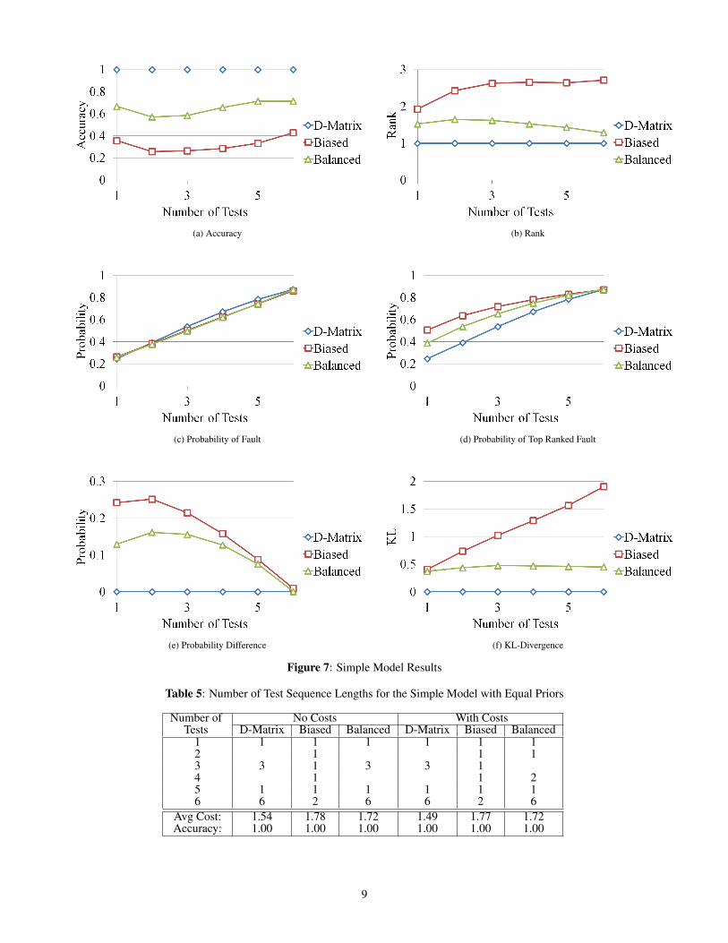
The accuracy-based results for the Simple Model are shownin Figure 7, and the corresponding results for the MissileModel are shown in Figure8. In the figures, “D-Matrix”denotes the Bayesian network derived from the full D-Matrixwhile “Biased” and “Balanced” denote the Bayesian net-works derived from the based and balanced trees, respec-tively.

Here we see that the D-Matrix models always correctlydiagnose the expected faults, thereby justifying their use forground truth. This is because each model has all of thelinks from the D-Matrix, so any assignment of tests willalways raise the probability of the correct fault. In the SimpleModel, the Balanced network performed second best withthe Biased network performing the worst. However, in theMissile Models, the performance of the Biased and Balancednetworks are almost the same for test sequences of length 4to 15. In the Simple Model, the performance of the Biasedand Balanced networks degrades from running only 1 test torunning 2 tests but then slowly improves. Meanwhile, the

accuracy of the Biased and Balanced networks for the MissileModel decreases dramatically from about 1 to 4 tests in thesequence and slowly increases as more tests are performed.

We see a similar set of results for the average Rank in Figures7b and 8b, where the D-Matrix always ranks the correctfault either first or in the top ambiguity group. In addition,the Biased network performs the worst while the Balancednetwork performs second best. For the Biased and Balancednetworks derived from the Missile Model, the average rankof the correct fault increases as more tests are performed upto 8 tests, as which point the rank begins to decrease.

When considering the probability of the correct fault on theSimple network, the highest ranked fault, and the differencebetween the two are shown in Figures 7c, 7d, and 7e. Theprobability of the correct fault increases in a linear fashionfor both the D-Matrix, Biased, and Balanced networks. Forthe Biased and Balanced networks, the probability of thetop ranked fault is higher than that of the correct fault butthen slowly levels out. In particular, this can be seen whenlooking at the probability difference. The results for theMissile Model, shown in Figures 8c, 8d, and 8e, are verysimilar to that of the Simple Model. The probability of thecorrect fault increases linearly for the D-Matrix, Biased, andBalanced networks while the probability for the top rankedfault increases in a logarithmic fashion for the Biased andBalanced networks. The probability difference results showan increase in the difference between the correct fault andtrue fault in test sequences of length 1 to 5, but then a steadydecrease occurs in sequences from 6 to 16 to tests.

Finally, we have the KL-Divergence results for the SimpleModel in Figure 7f and the Missile Model in Figure 8f. Basedon these results, we can see that the Balanced network’sdistribution is closer to that of the D-Matrix network thanthat of the Biased network for both the Simple and MissileModels. In addition, the difference between the distributionsincreases as the number of tests run is increased.

Degradation of Models Results

The results for the model degradation experiments are shownin Figure 9. Here, the x-Axis indicates the percent of thelinks that have been removed from the D-Matrix model. InFigure 9a we see that, as we remove links from the network,the accuracy decreases. In addition, the rank (Figure 9b)increases as the number of links are removed. Finally, we seethat the KL-Divergence (Figure 9c) increases as the numberof links are removed.

Average Costs

For the final set of experiments, we show the accuracy andthe average cost of the test sequences. In addition, we reporton the counts of the number of test sequence lengths, whichallows a user to see the distribution of tests that need to beperformed. Table 5 shows the sequence lengths and the num-ber of sequences of length x for both test selection methods,along with the average test sequence cost and accuracy forthe Simple Models. Table 6 shows the same results for thesenetworks; however, these networks do not have equal priorson the faults.

As shown in Table 5, the distribution of the sequence lengthsdoes not appreciably when comparing the test selection meth-ods. However, including test cost in the selection processdoes yield a slightly lower average cost (as one would ex-pect).

8

(a) Accuracy (b) Rank

(c) Probability of Fault (d) Probability of Top Ranked Fault

(e) Probability Difference (f) KL-Divergence

Figure 7: Simple Model Results

Table 5: Number of Test Sequence Lengths for the Simple Model with Equal Priors

Number of No Costs With CostsTests D-Matrix Biased Balanced D-Matrix Biased Balanced

1 1 1 1 1 1 12 1 1 13 3 1 3 3 14 1 1 25 1 1 1 1 1 16 6 2 6 6 2 6

Avg Cost: 1.54 1.78 1.72 1.49 1.77 1.72Accuracy: 1.00 1.00 1.00 1.00 1.00 1.00

9

(a) Accuracy (b) Rank

(c) Probability of Fault (d) Probability of Top Ranked Fault

(e) Probability Difference (f) KL-Divergence

Figure 8: Missile Model Results

Table 6: Number of Test Sequence Lengths for the Simple Model with Unequal Priors

Number of No Costs With CostsTests D-Matrix Biased Balanced D-Matrix Biased Balanced

1 1 1 12 1 1 1 2 13 3 1 5 3 1 34 2 1 4 1 15 1 1 5 1 16 1 2 4 6 2 2

Avg Cost: 1.99 1.58 1.95 1.91 1.58 1.98Accuracy: 1.00 0.80 0.86 1.00 0.80 0.86

10

(a) Accuracy

(b) Rank

(c) KL-Divergence

Figure 9: Degradation Results for the Simple Model.

When the priors of the faults are unequal (Table 6), theaverage cost of a test sequence increases for the D-Matrix andBalanced networks while decreasing for the Biased network.In addition, the Biased and Balanced networks no longerperform with 100 percent accuracy. Another interesting resultis that the average cost of the test sequences for the Biasednetwork is the same regardless of the test selection method.We also see that the difference between the average cost forthe two test selection methods on the D-Matrix and Balancedis very small.

The results for the Missile Models with equal priors areshown in Table 7 while the Missile Model results with non-equal priors are in Table 8. With equal priors, there isno difference between the two test selection methods. Inaddition, for all of the models, all 16 tests had to be performed

since the difference between the top ranked fault and thesecond top ranked fault never exceeded the threshold. Whena lower threshold was used, we encountered a problem thatsome faults were never diagnosed because the stop criterionwas met too early. Finally, the accuracy of the networks islower for the networks with unequal priors because a faultwith a low probability for a prior is harder to diagnose.

6. CONCLUSIONSIn this paper, we explored a procedure for deriving Bayesiannetworks from Fault Isolation Manuals (fault trees) and inves-tigated the accuracy of this procedure. From our experiments,we can conclude that deriving Bayesian networks from faulttrees will not perform as well as Bayesian networks derivedfrom the full D-Matrix because there are links missing in theBayesian network. This is not surprising; however, this is thefirst study to our knowledge that attempts to explore this issuein a systematic way.

Despite the fact that the Bayesian networks derived fromFIMs do not perform as well as the Bayesian network derivedfrom D-Matrices, there are several encouraging results. First,the average rank of the correct fault in the Simple Model wasaround 2.5 and 1.5 for the Biased and Balanced networksdepending on how many tests were run. Additionally, theranks for the Biased and Balanced networks for the MissileModel were between 2 and 4.5. While the ranks for Biasedand Balanced networks in the Missile Model were worsethan that for the Simple Model, there are more than twiceas many faults in the Missile Model than there are in theSimple Model. This shows that, while the correct fault maynot be ranked the highest, it is still ranked relatively high inthe overall list. This fits with what we would expect since inthe full D-Matrix, not all of the tests need to be performed todiagnose a fault.

Another encouraging result is that the probability of thehighest ranked fault and the true fault was relatively small,especially as the number of tests performed was increased.This shows us that while the correct fault may be ranked inthe top three, the difference between those top three faultsis relatively small. If a maintainer was using a Bayesiannetwork instead of a FIM, he or she would probably repairall three if the difference between the top candidates was solittle (as if they belonged to an ambiguity group). As analternative, the maintainer could choose to run more tests tofurther isolate the fault in the system.

We also noted some interesting results from the results onaccuracy. The first is that the probability of the top rankedfault for the Biased and Balanced networks was on averagehigher than that of the D-Matrix network. This was becausethe Biased and Balanced networks were missing links fromthe faults to the test nodes. Because of these missing links,the influence of the tests performed were stronger relative tofaults connected to those tests.

From the degradation results, we see that the performanceof the Bayesian network degrades fairly quickly when thefirst set of links are removed (20 percent of the links areremoved) and then performance seems to level out (fromabout 20 to 60 percent). We also noticed that the accuracyof the networks remains steady from 60 to 80 percent andeven increases in performance at the end. We also foundthat the graphs for Rank and KL-Divergence show a similarbehavior. The difference in KL-Divergence between the

11

Table 7: Number of Test Sequence Lengths for the Missile Model with Equal Priors

Number of No Costs With CostsTests D-Matrix Biased Balanced D-Matrix Biased Balanced

16 19 19 19 19 19 19Avg Cost: 22.50 22.50 22.50 22.50 22.50 22.50Accuracy: 1.00 0.50 0.45 1.00 0.50 0.45

Table 8: Number of Test Sequence Lengths for the Missile Model with Unequal Priors

Number of No Costs With CostsTests D-Matrix Biased Balanced D-Matrix Biased Balanced

16 19 19 19 19 19 19Avg Cost: 22.50 22.50 22.50 22.50 22.50 22.50Accuracy: 1.00 0.42 0.38 1.00 0.42 0.38

full D-Matrix network and the D-Matrix with links removeddegrades fairly steadily until about 60 percent of the linkshave been removed, at which point the difference levels outand even starts to reduce at the end.

In the final set of experiments that evaluate test cost andsequence length, we see that while we can still get decentperformance from the Biased and Balanced networks, thenetworks derived from the trees are not as cost efficient.While the distribution of the sequence lengths is fairly even,the average cost for the D-Matrix network was almost alwayslower than the two other networks, especially when costswere incorporated into the test selection process. We alsosee in the Missile Model that using a hard threshold of whento stop performing tests is not a good stopping criterion. Inthe Missile Model, all of the test sequences used all of thetests. However, in certain cases one could stop performingtests sooner, but determining when those cases occur is not atrivial task. This may suggest a variable approach to stoppingsuch as that described in [25].

7. SUMMARYIn this paper, we empirically analyzed the performance ofbipartite Bayesian networks that were derived from FIMs.While the derived Bayesian networks do not always ac-curately diagnose the correct fault, they still can performreasonably well when looking at some of the other results,such as the average probability of the correct fault. However,the Bayesian networks derived from the FIMs will not be ascost effective.

Using Bayesian networks for diagnosis offer several advan-tages. The first is that they allow for a natural extension fordiagnostic model maturation [26]. In our previous work wefocused on maturing D-Matrices and TFPGs. That work caneasily be extended to maturing bipartite Bayesian networkssince we can use historical maintenance and test sessiondata to learn new relationships and conditional probabilitiesbetween faults and tests. This will then allow us to learn bothif there is an erroneous relationship between a fault and alarmor to fill in the gap where a relationship was not previouslyknown to exist.

For future work, we plan to examine and develop approachesto mature the Bayesian networks derived from the FIMs.By developing an efficient approach to mature the networks,we would then be better able to justify converting FIMs toBayesian networks in the first place. This way we can make

use of the engineering expertise that generated the FIMs inthe first place as well as providing a seamless approach tomaturing the processes based on historical data.

ACKNOWLEDGMENTSThe authors would like to thank Boeing Research & Tech-nology for their support and guidance in work related tothis project. Without their guidance and direction this paperwould not have been possible. The authors would also liketo thank the members of the Numerical Intelligent SystemsLaboratory (NISL) at Montana State University for theirreviews and comments as the work unfolded as as earlierdrafts of the paper were prepared.

REFERENCES[1] W. Simpson and J. Sheppard, System test and diagnosis.

Norwell, MA: Kluwer Academic Publishers, 1994.

[2] T. M. Bearse, “Deriving a diagnostic inference modelfrom a test strategy,” in Research Perspectives and CaseStudies in System Test and Diagnosis, ser. Frontiers inElectronic Testing, J. W. Sheppard and W. R. Simpson,Eds. Springer US, 1998, vol. 13, pp. 55–67.

[3] P. Utgoff, “Incremental induction of decision trees,”Machine Learning, vol. 4, no. 2, pp. 161–186, 1989.

[4] F. Sahin, M. Yavuz, Z. Arnavut, and O. Uluyol, “Faultdiagnosis for airplane engines using bayesian networksand distributed particle swarm optimization,” ParallelComputing, vol. 33, no. 2, pp. 124–143, 2007.

[5] Z. Yongli, H. Limin, and L. Jinling, “Bayesiannetworks-based approach for power systems fault diag-nosis,” Power Delivery, IEEE Transactions on, vol. 21,no. 2, pp. 634–639, 2006.

[6] A. Bobbio, L. Portinale, M. Minichino, and E. Cian-camerla, “Improving the analysis of dependable systemsby mapping fault trees into bayesian networks,” Relia-bility Engineering & System Safety, vol. 71, no. 3, pp.249–260, 2001.

[7] S. Montani, L. Portinale, and A. Bobbio, “Dynamicbayesian networks for modeling advanced fault tree fea-tures in dependability analysis,” in Proceedings of thesixteenth European conference on safety and reliability,2005, pp. 1415–22.

[8] S. Montani, L. Portinale, A. Bobbio, and D. Codetta-

12

Raiteri, “Automatically translating dynamic fault treesinto dynamic bayesian networks by means of a softwaretool,” in Availability, Reliability and Security, 2006.ARES 2006. The First International Conference on.IEEE, 2006, pp. 6–pp.

[9] G. Hulten, D. Chickering, and D. Heckerman, “Learn-ing bayesian networks from dependency networks: apreliminary study,” in Proceedings of the Ninth Interna-tional Workshop on Artificial Intelligence and Statistics,2003.

[10] T. Jaakkola and M. I. Jordan, “Variational ProbabilisticInference and the QMR-DT Network,” JOURNAL OFARTIFICIAL INTELLIGENCE RESEARCH, vol. 10,pp. 291–322, 1999.

[11] S. Wahl and J. W. Sheppard, “Extracting decision treesfrom diagnostic bayesian networks to guide test se-lection,” in Annual Conference of the Prognostics andHealth Management Society, 2010.

[12] J. Sheppard and W. Simpson, “Fault diagnosis undertemporal constraints,” in AUTOTESTCON Proceedings,19921. IEEE Systems Readiness Technology Confer-ence, Sep. 1992, pp. 151–157.

[13] P. Ryan and W. Kent Fuchs, “Dynamic fault dictionariesand two-stage fault isolation,” Very Large Scale Integra-tion (VLSI) Systems, IEEE Transactions on, vol. 6, no. 1,pp. 176–180, Mar. 1998.

[14] N. H. Narayanan and N. Viswanadham, “A methodol-ogy for knowledge acquisition and reasoning in failureanalysis of systems,” IEEE Trans. Syst. Man Cybern.,vol. 17, pp. 274–288, March 1987.

[15] S. Abdelwahed, G. Karsai, and G. Biswas, “Aconsistency-based robust diagnosis approach for tempo-ral causal systems,” in The 16th International Workshopon Principles of Diagnosis, 2005, pp. 73–79.

[16] K. Przytula and D. Thompson, “Construction ofbayesian networks for diagnostics,” in Aerospace Con-ference Proceedings, 2000 IEEE, vol. 5. IEEE, 2000,pp. 193–200.

[17] J. W. Sheppard and S. G. Butcher, “A formal analysisof fault diagnosis with d-matrices,” J. Electron. Test.,vol. 23, pp. 309–322, aug. 2007.

[18] E. Alpaydin, Introduction to Machine Learning (Adap-tive Computation and Machine Learning). The MITPress, 2010.

[19] P. Utgoff, N. Berkman, and J. Clouse, “Decision treeinduction based on efficient tree restructuring,” MachineLearning, vol. 29, no. 1, pp. 5–44, 1997.

[20] D. Koller and N. Friedman, Probabilistic GraphicalModels: Principles and Techniques. MIT Press, 2009.

[21] J. Pearl, Probabilistic reasoning in intelligent systems:networks of plausible inference. San Francisco, CA,USA: Morgan Kaufmann Publishers Inc., 1988.

[22] G. Cooper, “The computational complexity of proba-bilistic inference using bayesian belief networks,” Ar-tificial intelligence, vol. 42, no. 2, pp. 393–405, 1990.

[23] D. S. L. of the University of Pittsburgh. [Online].Available: http://genie.sis.pitt.edu/

[24] C. Huang and A. Darwiche, “Inference in belief net-works: A procedural guide,” International journal ofapproximate reasoning, vol. 15, no. 3, pp. 225–263,1996.

[25] J. Sheppard, W. Simpson, and J. Graham, “Methodand apparatus for diagnostic testing including a neuralnetwork for determining testing sufficiency,” Jul. 141992, US Patent 5,130,936.

[26] S. Strasser and J. Sheppard, “Diagnostic alarm sequencematuration in timed failure propagation graphs,” inIEEE AUTOTESTCON Conference Record, 2011, pp.158–165.

BIOGRAPHY[

Shane Strasser received a BS in com-puter science and mathematics from theUniversity of Sioux Falls in Sioux Falls,South Dakota. Afterwards he went onto obtain an MS in Computer Science atMontana State University, where he iscurrently working on his PhD in Com-puter Science. While at Montana State,he has received several awards, such asthe 2012 outstanding PhD MSU Com-

puter Science researcher and the 2011 AUTOTESTCON BestStudent Paper Award. His research interests are primarily inartificial intelligence and machine learning with a focus onprognostics and health management systems. In his free timehe enjoys singing, running, and riding motorcycles.

John Sheppard was the inauguralRightNow Technologies DistinguishedProfessor in Computer Science at Mon-tana State University and currently holdsan appointment as Professor in the Com-puter Science Department at MSU. He isalso an Adjunct Professor in the Depart-ment of Computer Science at Johns Hop-kins University. He holds a BS in com-puter science from Southern Methodist

University and an MS and PhD in computer science, bothfrom Johns Hopkins University. In 2007, he was elected asan IEEE Fellow “for contributions to system-level diagnosisand prognosis.” Prior to joining Hopkins, he was a Fellowat ARINC Incorporated in Annapolis, MD where he workedfor almost 20 years. Dr. Sheppard performs research inBayesian classification, dynamic Bayesian networks, evolu-tionary methods, and reinforcement learning. In addition, Dr.Sheppard is active in IEEE standards activities. Currently, heserves as a member of the IEEE Computer Society StandardsActivities Board and is the Computer Society liaison to IEEEStandards Coordinating Committee 20 on Test and Diagnosisfor Electronic Systems. He is also the co-chair of the Di-agnostic and Maintenance Control Subcommittee of SCC20and has served as an official US delegate to the InternationalElectrotechnical Commission’s Technical Committee 93 onDesign Automation.

13