an empirical evaluation of accounting income numbers

An Empirical Evaluation of AccountingIncome Numbers

RAY BALL* and PHILIP BROWNt

Accounting theorists have generally evaluated the usefulness of account• ing practices by the extent of their agreement with a particular analytic model. The model may consist of only a few assertions or it may be a rigorously developed argument. In each case, the method of evaluation has been to compare existing practices with the more preferable practices im• plied by the model or with some standard which the model implies all practices should possess. The shortcoming of this method is that it ignores a significant source of knowledge of the world, namely, the extent to which the predictions of the model conform to observed behavior.

It is not enough to defend an analytical inquiry on the basis that its assumptions are empirically supportable, for how is one to know that a theory embraces all of the relevant supportable assumptions? And how does one explain the predictive powers of propositions which are based on un• verifiable assumptions such as the maximization of utility functions? Further, how is one to resolve differences between propositions which arise from considering different aspects of the world?

The limitations of a completely analytical approach to usefulness are il•lustrated by the argument that income numbers cannot be defined sub•stantively, that they lack "meaning" and are therefore of doubtful utility.1

The argument stems in part from the patchwork development of account-

*University of Chicago. t University of Western Australia. The authors are indebted to the participants in the Workshopin AccountingResearch at the Univer• sity of Chicago, Professor Myron Scholes, and Messrs. OwenHewett and Ian Watts.

1 Versions of this particular argument appear in Canning (1929); Gilman (1939); Paton and Littleton (194-0); Vatter (1947), Ch. 2; Edwards and Bell (1961), Ch. l; Chambers (1964), pp. 267-68; Chambers (1966), pp. 4 and 102; Lim (1966), esp. pp. 645and 649; Chambers (1967), pp. 745-55; Ijiri (1967), Ch. 6, esp. pp. 120-31; and Sterling(1967), p. 65.

159

160 JOURNAL OF ACCOUNTING RlUSEARCH, AUTUMN, 1968

ing practices to meet new situations as they arise. Accountants have had to deal with consolidations, leases, mergers, research and development, price-• level changes, and taxation charges, to name just a few problem areas. Because accounting lacks an all-embracing theoretical framework, dissimi• larities in practices have evolved. As a consequence, net income is an ag• gregate of components which are not homogeneous. It is thus alleged to be a "meaningless" figure, not unlike the difference between twenty-seven tables and eight chairs. Under this view, net income can be defined only asthe result of the application of a set of procedures f X 1 , X2 , · · · } to a set of events { Y1, Y2, · · ·} with no other definitive substantive meaning at all.Canning observes:

What is set out as a measure of net income can never be supposed to be a fact in any sense at all except that it is the figure that results when the accountant has finished applying the procedures which he adopts.1

The value of analytical attempts to develop measurements capable of definitive interpretation is not at issue. What is at issue is the fact that an analytical model does not itself assess the significance of departures from its implied measurements. Hence it is dangerous to conclude, in the absence of further empirical testing, tha't a lack of substantive meaning implies a lack of utility.

An empirical evaluation of accounting income numbers requires agree•ment as to what real-world outcome constitutes an appropriate test of use• fulness. Because net income is a number of particular interest to investors, the outcome we use as a predictive criterion is the investment decision as it is reflected in security prices.3 Both the content and the timing of existing annual net income numbers will be evaluated since usefulness could be im• paired by deficiencies in either.

An Empirical Test

Recent developments in capital theory provide justification for selecting the behavior of security prices as an operational test of usefulness. An im• pressive body of theory supports the proposition that capital markets are both efficient and unbiased in that if information is useful in forming capital asset prices, then the market will adjust asset prices to that information quickly and without leaving any opportunity for further abnormal gain. 4

If, as the evidence indicates, security prices do inf act' adjust rapidly to newinformation as it becomes available, then changes in security prices will re-

t Canning (1929), p. 98.•Another approach pursued by Beaver (1968) is to use the investment decision,

as it is reflected in transactions volume, for a. predictive criterion.'For example, Samuelson (1965) demonstrated that a market without bias in its

evaluation of information will give rise to randomly fluctuating time series of prices. See also Cootner (ed.) (1964); Fama (1965); Fama and Blume (1966); Fama, et al.(1967); and Jensen (1968).

EMPIRICAL EVALUATION OF ACCOUNTING INCOME NUMBERS 161

fleet the flow of information to the market.5 An observed revision of stock prices associated with the release of the income report would thus provide evidence that the information reflected in income numbers is useful.

Our method of relating accounting income to stock prices builds on this theory and evidence by focusing on the information which is unique to a particular firm.11 Specifically, we construct two alternative models of what the market expects income to be and then investigate the market's reac• tions when its expectations prove false.

ElXPE;.<JTED Ai.~ UNEXPECTED INCOME CHANGES

Historically, the incomes of firms have tended to move together. One study found that about half of the variability in the level of an average firm's earnings per share (EPS) could be associated with economy-wide effects," In light of this evidence, at least part of the change in a firm's in• come from one year to the next is to be expected. H, in prior years, the in• come of a firm has been related to the incomes of other firms in a particular way, then knowledge of that past relation, together with a knowledge of the incomes of those other firms for the present year, yields a conditional ex• pectation for the present income of the firm. Thus, apart from confirmation effects, the amount of new information conveyed by the present income number can be approximated by the difference between the actual change in income and its conditional expectation.

But not all of this difference is necessarily new information. Some changes in income result from financing and other policy decisions made by the firm. We assume that, to a first approximation, such changes are reflected in the average change in income through time.

Since the impacts of these two components of change--economy-wide and policy effects-are felt simultaneously, the relationship must be esti• mated jointly. The statistical specification we adopt is first to estimate, by Ordinary Least Squares (OLS), the coefficients (a1;c , aa;c) from the linear regression of the change in firm j's income (Al;,e-r) on the change in the average income of all firms (other than firm J) in the market (LlM;.e-r)8

using data up to the end of the previous year (T = 1, 2, · · · , t - 1):

T = 1, 2, • • · 7 t - 1, (1)

6 One well documented characteristic of the security market is that useful sources of information are acted upon and useless sources are ignored. This is hardly surpris• ing since the market consists of a. large number of competing actors who can gain from acting upon better interpretations of the future than those of their rivals. See, for example, Scholes (1967);and footnote 4 above. This evaluation of the security market differs sharply from that of Chambers (1966, pp. 272-73).

6 More precisely, we focus on information not common to all firms, since some in•dustry effects are not considered in this paper.

1 Alternatively, 35 to 40 per cent could be associated with effects common to all firms when income was defined as tu-adjusted Return on Capital Employed. [Source: Ball and Brown (1967), Table 4.)

a We call Ma "market index" of income because it is constructed only from firms traded on the New York Stock Exchange.

162 RAY BALL AND PWLIP BROWN

where the hats denote estimates. The expected income change for firm j in year t is then given by the regression prediction using the change in the average income for the market in yese t:

Al;c = d1;e + °'2;tAilf ;c •

The unexpected income change, or forecast error (u;,), is the actual income change minus expected:

(2)

It is this forecast error which we assume to be the new information con•veyed by the present income number.

THE MARKET'S REACTION

It has also been demonstrated that stock prices, and therefore rates of return from holding stocks, tend to move together. In one study," it was estimated that about 30 to 40 per cent of the variability in a stock's monthly rate of return over the period March, 1944 through December, 1960 could be associated with market-wide effects. Market-wide variations in stock returns are triggered by the release of information which concerns all firms. Since we are evaluating the income report as it relates to the individual firm, its contents and timing should be assessed relative to changes in the rate of return on the firm's stocks net of market-wide effects.

The impact of market-wide information on the monthly rate of return from investing one dollar in the stock of firm j may be estimated by its predicted value from the linear regression of the monthly price relatives of firm j's common stock10 on a market index of returns :11

t King (1966).10 The monthly price relative of security j for month m is defined as dividends

(dim) + closing price <P1,m+1), divided by opening price (p;m):

PR;m = <Pi.m+l + d1m)IP1m.

A monthly price relative is thus equal to the discrete monthly rate of return plus unity; its natural logarithm is the monthly rate of return compounded continuously. In this paper, we assume discrete compoundingsince the results are easier to inter• pret in that form.

11 Fama, et al. (1967)conclude that "regressionsof security on market returns over time are a satisfactory method for abstracting from the effects of general marketconditions on the monthly rates of return on individual securities." In arriving at their conclusion, they found that "scatter diagrams for the [returns on] individual securities [vis-A-vis the market return} support very well the regression assumptions of linearity, homoscedaaticity, and serial independence." Fama, et al. studied the natural logarithmic transforms of the price relatives, as did King (1966).However, Blume (1968)worked with equation (3). We also performed tests on the alternativespecification:

(3a)

where In, denotes the natural logarithmic function. The results correspond closely with those reported below.

EMPIRICAL EVALUATION OJ' ACCOUNTING INCOME NUMBERS 163

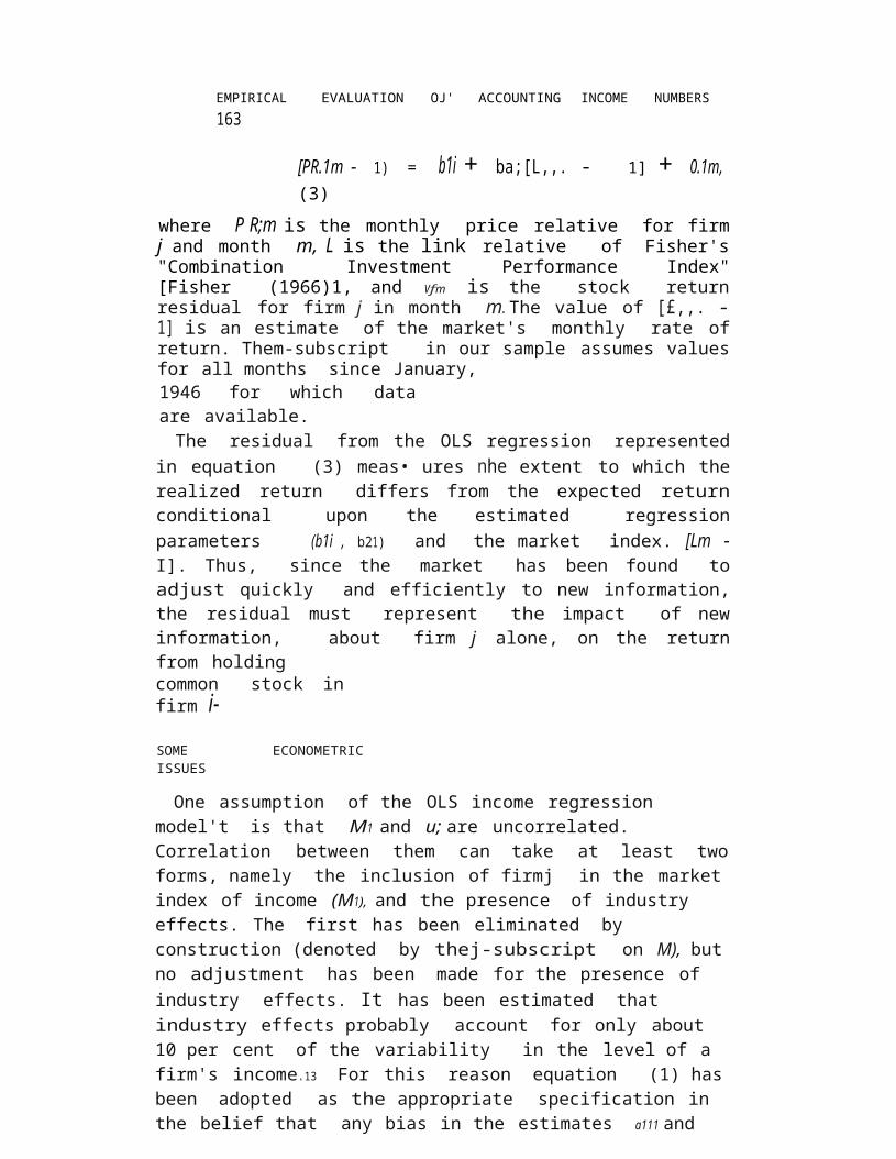
[PR.1m - 1) = b1i + ba;[L,,. - 1] + 0.1m, (3)

where P R;m is the monthly price relative for firm j and month m, L is the link relative of Fisher's "Combination Investment Performance Index" [Fisher (1966)1, and Vfm is the stock return residual for firm j in month m. The value of [£,,. - 1] is an estimate of the market's monthly rate of return. Them-subscript in our sample assumes values for all months since January,1946 for which data are available.

The residual from the OLS regression represented in equation (3) meas• ures nhe extent to which the realized return differs from the expected return conditional upon the estimated regression parameters (b1i , b21) and the market index. [Lm - I]. Thus, since the market has been found to adjust quickly and efficiently to new information, the residual must represent the impact of new information, about firm j alone, on the return from holdingcommon stock in firm i-

SOME ECONOMETRIC ISSUES

One assumption of the OLS income regression model't is that M1 and u; are uncorrelated. Correlation between them can take at least two forms, namely the inclusion of firmj in the market index of income (M1), and the presence of industry effects. The first has been eliminated by construction (denoted by thej-subscript on M), but no adjustment· has been made for the presence of industry effects. It has been estimated that industry effects probably account for only about 10 per cent of the variability in the level of a firm's income.13 For this reason equation (1) has been adopted as the appropriate specification in the belief that any bias in the estimates a111 and~it will not be significant. However, as a check on the statistical efficiencyof the model, we also present results for an alternative, naive model which predicts that income will be the same for this year as for last. Its forecast error is simply the change in income since the previous year.

As is the case with the income regression model, the stock return model, as presented, contains several obvious violations of the assumptions of the OLSregression model. First, the market index of returns is correlated with the residual because the market index contains the return on firm i. and be• cause of industry effects. Neither violation is serious, because Fisher's index is calculated over all stocks listed on the New York Stock Exchange (hence the return on security j is only a small part of the index), and because in•dustry effects account for at most 10 per cent of the variability in the rate

11 That is, an assumption necessary for OLS to be the minimum-variance, linear, unbiased estimator.

13 The magnitude assigned to industry effects depends upon how broadly an indus•try is defined, which in tum depends upon the particular empirical application beingconsidered. The estimate of 10 per cent is bssed on a two-digit classification scheme. There is some evidence that industry effects.might account for more than 10 per cent when the association is estimated in first differences [Brealey (1968)].

164 RAY BALL Al.'i'D PHILIP BROWN

of return on the average stock.14 A second violation results from our predic• tion that, for certain months around the report dates, the expected values of the are nonzero. Again, a;ny bias should have little effect on the re• sults, inasmuch as there is a low, observed autocorrela.tionin the D/s,16 and in no case was the stock return regressionfitted over less than 100 observa• tions."

SUMMARY

We assume that in the unlikely absence of useful inform.ation about a. particular firm. over a period, its rate of return over that period would re• flect only the presence of market-wide information which pertains to all firms. By abstracting from market effects [equation (3)1 we identify the effect of informstion pertaining to individual firms. Then, to determine if part of this effect can be associated with inf ormation contained in the firm's accounting income number, we segregate the expected and unexpected elements of income change. If the income forecast error is negative (that is> if the actual change in income is less than its conditional ex:pootation),we define it as bad news and predict that if there is some association between accounting income numbers and stock prices, then release of the income number would result in the return on that firm's securities being less than

1• The estim,ate of 10 per cent is due to King (1966). Blume (1968) has recently questioned the magnitude of industry effects, suggesting that they could be somewhat less than 10 per cent. His contention is based on the observation that the significance. attached to industry effects depends on the assumptions made about the parameters. of the distributions underlying stock rates of return.

15 See Table 4, below.111 Fa.ma, et al. (1967) faced a similar situation. The expected values of the stock

return residuals were nonzero for some of the months in their study. Stock return regressions were calculated separately for both exclusion and inclusion of the months for which the stock return residuals were thought to be nonzero. They report thatboth. sets of results support the same conclusions.

An altemative to constraining the mean Vi to be zero is to employ the Sharpe Capi•tal Asset Pricing Model [Sharpe (1964)) to estimate (3b):

PR1m - RF. - 1 = b;; + ~; [L,,. - RF,,. - 1) + v;., (3b}

where RF is the risk-free ex ante rate of return for holding period m. Results from estimating (3b) (using U.S. Government Bills to measure RF' and defining the abnor•mal return for firm fin month m now as b~; + vi.,.) are essentially the same as theresults from (3).

Equation (Sb) is still not entirely satisfactory, however, since the mean impactof new infomiation is estimated over the whole history of the stock, which. covers at least 100 months. If (~b) were fitted using monthly data, a vector of dummy variables could be introduced to identify the fiscal year covered by the annual report, thus permitting the mean residual to vary between fiscal years. The impact of unusual information received i:p month m of year t would then be estimated by the sum of theconstant, the dummyfor year t, a;nd the calculated residual for :month m and year t,Unfortunatel:y, the eftici.enc;yof estimating the stock return equation in this partic•ular form has not been investigated satisf actorily, hence our report will be confinedto the results from estimating (3).

-

1EMPIRICAL EVALUATION OF ACCOUNTING INCOME

TABL 1

1 RAY BALL AND PHILIP

Decilea of tM Diatributiona of Squared Coefficients of Correlationt C1w,-nge8 in Firm and Market Income*

VariableDecile

.1 .2 .3 .4 .5 .6 .7 .8 .9

-- -- -- -- -- -- --(1) Net income ........ .03 .07 .10 .15 .23 .30 .35 .43 .52

(2) EPS .............. .02 .05 .11 .16 .23 .28 .35 .42 .52

* Estimated over the 21 years, 1946-1966.

would otherwise have been expected.17 Such a result (tl < O) would be evi• denced by negative behavior in the stock return residuals (IJ < 0) around the annual report announcement date. The converse should hold for a positive forecast error.

Two basic income expectations models have been defined, a regression model and a naive model. We report in detail on two measures of income

"[net income and EPS, variables (I) and (2)] for the regression model, andone measure [EPS, variable (3)] for the naive model.

DataThree classes of data are of interest: the contents of income reports; the

dates of the report announcements; and the movements of security prices around the announcement dates.

INCOME NUMBERS

Income numbers for 1946 through 1966 were obtained from Standard and Poor's Compustat tapes.18 The distributions of the squared coefficients of correlation19 between the changes in the incomes of the individual firms and the changes in the market's income index20 are summarized in Table 1. For the present sample, about one-fourth of the variability in the changes

11 We later divide the total return into two parts: a "normal return," defined by the return which would have been expected given the normal relationship between a stock and the market index; and an "abnormal return," the difference between theactual return and the normal return. Formally, the two parts are given by: b 11 +bi; [L,,. - 1]; and Vfm.

is Tapes used are dated 9/28/1965 and 7/07/1967.n All correlation coefficients in this paper are product-moment correlation coeffi•

cients.2• The market net income index was computed as the sample mean for each year.

The market EPS index was computed as a weighted average over the sample members,the number of stocks outstanding (adjusted for stock splits and stock dividends) providing the weights. Note that when estimating the asaoeiation between the income of a particular firm and the market, the income of that firm was excluded from themarket index.

Decile

~·Variable

.1 .2 .J .4 .s .6 .7

(1) Net income... -.35 -.28 -.20 -.12 -.05 .02 .12(2) EPS .......... -.39 -.29 -.21 -.15 -.08 -.03 .07 .35


TABL 1


TABLE 2Decile8 of ths Di8tributiom of the Coefficient.a of Fir8t-Order Autocorrelation in the

Income Regres8ion Residuals*

.33

•Estimated over the 21years,1946-1966.

in the median firm's income can be associated with changes in the market index.

The association between the levels of the earnings of firms was examinedin the forerunner article [Ball and Brown (1967)]. At that time, we referredto the existence of autocorrelation in the disturbances when the levels of net income and EPS were regressed on the appropriate indexes. In this paper, the specification has been changed from levels to first differences because our method of analyzing the stock market's reaction to income numbers presupposes the income forecast errors to be unpredictable at a minimum of 12 months prior to the announcement dates. This supposition is inappropriate when the errors are autocorrelated.

We tested the extent of autocorrelation in the residuals from the incomeregression model after the variables had been changed from levels to first differences. The results are presented in Table 2. They indicate that the supposition is not now unwarranted.

ANNUAL REPORT ANNOUNCEMENT DATES

The Wall Street Journal publishes three kinds of annual report announce• ments: forecasts of the year's income, as made, for example, by corporation executives shortly after the year end; preliminary reports; and the com• plete annual report. While forecasts are often imprecise, the preliminary report is typically a condensed preview of the annual report. Because the preliminary report usually contains the same numbers for net income and EPS as are given later with the final report, the announcement date (or, effectively' the date on which the annual income number became generally available) was assumed to be the date on which the preliminary report appeared in the Wall Street Journal. Table 3 reveals that the time lag between the end of the fiscal year and the release of the annual report has been declining steadily throughout the sample period.

STOCK PRICES

Stock price relatives were obtained from the tapes constructed by theCenter for Research in Security Prices (CRSP) at the University of Chi-

•


TABLE


Time Distribution. of An?WUncem61Lt Date8

Percent of tinns

Fiscal year

1957 1958 1959 1960 1961 1962 1963 1964 1965

25 2/07• 2/04 2/04 2/03 2/02 2/05 2/03 2/01 1/3150 2/25 2/20 2/18 2/17 2/15 2/15 2/13 2/09 2/0875 3/10 3/06 3/04 3/03 3/05 3/04 2/28 2/25 2/21

a Indicates that 25 per cent of the income reports for the fiscal year ended 12/31/1957 had been announced by 2/07/1958.

TABLE 4Deciles of the Distributions of the Squared Coefficient of Correlation for the Stock Return Regression, and of the Coefficient of First-Order Autocorrelation in the

Stock Return Residuals•

Coefficientname

Decile

.1 .2 .J .4 .5 .s .7 .8 .9

Return re- gress•1onr ,• ..

Residual auto-

.18 .22 .25 .28 .31 .34 .37 .40 .46

correlation .. -.17 -.14 -.11 -.10 -.08 -.05 -.03 -.01 .03

•Estimated over the 246 months, January, 1946 through June, 1966.

cago.21 The data used are monthly closing prices on the New York Stock Exchange, adjusted for dividends and capital changes, for the period Janu• ary, 1946 through June, 1966. Table 4 presents the deciles of the distribu• tions of the squared coefficientof correlation for the stock return regression [equation (3)], and of the coefficient of first-order autocorrelation in the stock residuals.

INCLUSION CRITERIA

Firms included in the study met the following criteria:1. earnings data available on the Compustat tapes for each of the years

1946-1966;2. fiscal year ending December 31;3. price data available on the CRSP tapes for at least 100 months; and4. Wall Street Journal announcement dates availsble."Our analysis was limited to the nine fiscalyears 1957-1965. By

beginning the analysis with 1957, we were assured of at least 10 observations when

n The Center for Research in Security Prices at the University of Chicago is spon•sored by Merrill Lynch, Pierce, Fenner and Smith Incorporated.

22 Announcement dates were taken initially from the Wall Street Journal Index,then verified against the Wall Street Journal.


TABLE


estimating the income regression equations. The upper limit (the fiscal year 1965, the results of which are announced in 1966) is imposed because the CRSP file terminated in June, 1966.

Our selection criteria may reduce the generality of the results. The sub•population does not include young firms, those which have failed, thosewhich do not report on December 31, and those which are not represented on Compustai, the CRSP tapes, and the Wall Street Journal. As a result, it may not be representative of all firms. However, note that (1) the 261 remaining firms23 are significantin their own right, and (2) a replication of our study on a different sample produced results which conform closely to those reported below.24

Resulta

Define month 0 as the month of the annual report announcement, andAP IM , the Abnormal Perform.anceIndex at month M, as:

1 N M

APJM = N}: II (1 + Vnm)•n m-11

Then API traces out the value of one dollar invested (in equal amounts) in all securities n (n = 1, 2, · · · , N) at the end of month -12 (that is, 12 months prior to the month of the annual report) and held to the end ofsome arbitrary holding period (M = -11, -10, · · · , T) after abstracting from market affects. An equivalent interpretation is as follows. Suppose two individuals A and B agree on the followingproposition. B is to con• struct a portfolio consisting of one dollar invested in equal amounts in N securities. The securities are to be purchased at the end of month -12 and held until the end of month T. For some price, B contracts with A to take (or make up), at the end of each month M, only the normal gains (or losses)and to return to A, at the end of month T, one dollar plus or minus any abnormal gains or losses.Then API Mis the value of A's equity in the mutual portfolio at the end of each month M .26

Numerical results are presented in two forms. Figure 1 plots API M

first for three portfolios constructed from all firms and years in which the incomeforecast errors, accordingto each of the three variables,werepositive (the top half); second, for three portfolios of firms and years in which the income forecast errors were negative (the bottom half); and third, for a single portfolio consisting of all firms and years in the sample (the linewhich wanders just below the line dividing the two halves). Table 5 in•cludes the numbers on which Figure 1 is based.

ta Due to known errors in the data, not all fi..nns eould be included in all years. The fisesl year most affected was 1964, when three firms were excluded.

H The replication investigated 75 firms with fiscal yea.rs ending on dates otherthan December 31, using the naive income-forecasting model, over the longer period1947~65.

u That is, the value expected at the end of month Tin the absence of further ab·normal gains and losses.

Total sample. ~

EMPmICAL EVALUATION OF ACCOUNTING INCOME NUMBERS 169

U2

1.10

1.08

l.06

1.04

Variable 2

~..51.02

8c

0~ 1.00 NF---,.,.,,.~,....·--------...-....-..--.---.-...--.-. .----1r----------i.£.... ~..'...0 0.98 "':,. ..E <, .,0 ' ..

·····-........... .. 1···......... ··--..-·- _

~c0.96

0.94

0.92

0.90

0.88

'· "'\.

~""'........\.~

"'~.-.............,. ,.z-.,""·~,

"· ~... Variable J··~::::.-

··-._

,..::.,..-.::.:\-J--

Variable 2 F"

-12 -10 -8 -6 -4 -2 0 2 4 6Month Relative to Annual Report Announcement Date

Fro. 1 Abnormal Performance Indexes for Various Portfolios

Since the first set of results may be sensitive to the distributions of the stock return disturbancee.s a second set of results is presented. The third column under each variable heading in Table 5 gives the chi-square statistic for a two-by-two classification of firms by the sign of the income forecast error, and the sign of the stock return residual for that month.

OVERVIEW

As one would expect from a large sample, both sets of results convey essentially the same picture. They demonstrate that the information con• tained in the annual income number is useful in that if actual income differs

21 The empirical distributions of the stock return residuals appear to be described well by symmetric, stable distributions that are characterized by tails longer than those of the normal distribution [Fa.ma (1965); Fama, et al. (1967)].

saTot


TABLE 5

Summary Statistics bu l&lonth Relative to Annual Report Announcement Date

Month rela-Regression model Naive model

tive to annualreport an· Net income EPS EPS

nouneementdate

(1)" (2) (3) (1) (2) (3) (1) (2) (3)

--- ---11 1.006 .992 16.5 1.007 .992 20.4 1.006 .989 24.1 1.000-10 1.014 .983 17.3 1.015 .982 20.2 1.015 .972 73.4 .999-9 1.017 .977 7.9 1.017 .977 3.7 1.018 .965 20.4 .998-8 1.021 .971 9.5 1.022 .971 12.0 1.022 .956 9.1 .998

-7 1.026 .960 21.8 1.027 .960 27.1 1.024 .946 9.0 .995

-6 1.033 .949 42.9 1.034 .948 37.6 1.027 .937 19.4 .993-5 1.038 .941 17.9 1.039 .941 21.3 1.032 .925 21.0 .992-4 1.050 .930 40.0 1.050 .930 39.5 1.041 .912 41.5 .993-3 1.059 .924 35.3 1.060 .922 33.9 1.049 .903 37.2 .995-2 1.057 .921 1.4 1.058 .919 1.8 1.045 .903 0.1 .992-1 1.060 .914 8.2 1.062 .912 8.2 1.046 .896 5.7 .991

0 1.071 .907 28.0 1.073 .905 28.9 1.056 .887 35.8 .9931 1.075 .901 6.4 1.076 .899 5.5 1.057 .882 9.4 .9922 1.076 .899 2.7 1.078 .897 1.9 1.059 .878 8.1 .9923 1.078 .896 0.6 1.079 .895 1.2 1.059 .876 0.1 .9914 1.078 .893 0.1 1.079 .892 0.1 1.057 .876 1.2 .9905 1.075 .893 0.7 1.077 .891 0.1 1.055 .876 0.6 .9896 1.072 .892 o.o 1.074 .889 0.2 1.051 .877 0.1 .987

" Column headings:(1) Abnormal Performance Index-firms and years in which the income forecast

error was positive.(2) Abnormal Performance Index-firms and years in which the income forecast

error was negative.(3) Chi-square statistic for two-by-two classification by sign of income forecast

error (for the fiscal year) and sign of stock return residual (for the indicated month).

Note: Probability (chi-square ~ 3.84 I x.2 - 0) = .05, for 1 degree of freedom.Probability (chi-square ~ 6.64 Ix* ... 0) == .01, for 1 degree of freedom.

from expected income, the market typically has reacted in the same direc• tion. This contention is supported both by Figure l which reveals a marked, positive association between the sign of the error in forecasting income and the Abnormal Performance Index, and by the chi-square statistic (Table 5). The latter shows it is most unlikely that there is no relationship between the sign of the income forecast error and the sign of the rate of return re• sidual in most of the months up to that of the annual report announcement.

However, most of the information contained in reported income is an• ticipated by the market before the annual report is released. In fact, an• ticipation is so accurate that the actual income number does not appear to cause any unusual jumps in the Abnormal Performance Index in the an• nouncement month. To illustrate, the drifts upward and downward begin at least 12 months before the report is released (when the portfolios are first

a

EMPimCAL EVALUATION 01' ACCOUN'l'ING INCOMlil Nl11dlJEBS 171

T4:QL:E 6OonJing~ ~(4ble of tis 8i1111ia. oJ.Ou, Income For11~t /firtori-lJtl

.Variable

Sign ol bie~e forccut error

Variable (1)

Variable (1)

+ + +

+ 1231 1148

83 1074 157

«,

Variable (2)+

Variable (3)

+

1109 83

1231

1074 !

157 •.

1026 399

1074399.

1473

710

157710

867,. - -- .

:::_ ·.' . ,: i

constructed) and continue for approximately one month after. The persistence of . . • iC.ated by:the coristant si .• s of th~· indexes and by their in absolute v . . . ····.· 1), st.tggestsnot only.that . to !'llvicipateforec~.errors early in the 12 months prec :; but a.JS() that it. continiles to. so with in-

out the ve1c1:p ,,,,

,,.·. :- .-:.:· ... ;:.:•,-.:-,.,_,,.,_,:,

.. sPEC!wc RE8U~,··

L There appears to be littl~ difference between the results for the two· · a'bles. Tagle 6, wliich classifiesthe.sign of one variable's

....· .. upofi:the · .· of the errors bf the-Othertwo'vari-. F · · 1231 occasions on which the

>,'::

.eon, odthe

or was negative for variable

. r.varia'ble (2). The fact thathose for variable (1) suggests,

· on the sign of an income


(a) the change in market income were zero, and (b) there were no drift in the income of the firm. But historically there has been an increase· in the market's income, particularly during the latter part of the sample period, due to general increase in prices and the strong influence of the protracted expansion since 1961. Thus, the naive model [variable (3)] typically identi• fies as firms with negative forecast errors those relatively few firms which showed a decrease in EPS when most firms showed an increase. Of the three variables, one would be most confident that the incomesof those which showed negative forecast errors for variable (3) have in fact lost ground relative to the market.

This observation has interesting implications. For example, it points to arelationship between the magnitudes of the income forecast errors and themagnitudes of the abnormal stock price adjustments. This conclusion is reinforced by Figure 1 which shows that the results for positive forecast errors are weaker for variable (3) than for the other two.

2. The drift downward in the Abnormal Performance Index computed over all firms and years in the sample reflects a computational bias.28 The bias arises because

E[IJ (1 + Vm)] ~ IJ [1 + E(vm)],m "'

where E denotes the expected value. It can readily be seen that the bias over K months is at least of order (K - 1) times the covariance between Vm and Vm-1 •

29 Since this covariance is typically negative,30 the bias is also negative.

While the bias does not affect the tenor of our results in any way, itshould be kept in mind when interpreting the values of the various API's. It helps explain, for example, why the absolute changes in the indexes in the bottom panel of Figure 1 tend to be greater than those in the top panel; why the indexes in the top panel tend to turn down shortly' after month 0; and finally, why the drifts in the indexesin the bottom panel tend to persist beyond the month of the report announcement.

3. We also computed results for the regressionmodel using the additional definitions of income:

(a) cash flow, as approximated by operating income,31 and(b) net income before nonrecurring items.

Neither variable was as successfulin predicting the signs of the stock return

28 The expected value of the bias is of order minus one-half to minus one-quarter of one per cent per annum. The difference between the observed value of the API computed over the total sample and its expectation is a property of the particular sample (see footnote 26).

20 In particular, the approximation neglects all permutations of the prod•uct v,·v,, 8 = 1, 2, · · · , K-2, t = s+2, · · · , K, as being of a second order of smallness.

31J See Table 4.31 All variable definitions are specified in Standard and Poor's Comqnistat Manual

[see also Ball and Brown (1967), Appendix A].

+

EMPmICAL EVALUATION OF ACCOUNTING il~COME NUMBERS 173

residuals M net income and EPS. For example, by month 0, the Abnormal Performance Indexes for forecast errors which were positive were 1.068 (net income, including nonrecurring items) and 1.070 (operating income). These numbers compare with 1.071 for net income [Table 5, variable (1)]. The respective numbers for firms and years with negative forecast errors were 0.911, 0.917, and 0.907.

4. Both the API's and the chi-square test in Table 5 suggest that, at least for variable (3), the relationship between the sign of the income fore• cast error and that of the stock return residual may have persisted for M

longas two months beyond the month of the announcement of the annual report. One explanation might be that the market's index of income WM

not known for sure until after several firms had announced their income numbers. The elimination of uncertainty about the market's income subse• quent to some firms' announcements might tend, when averaged over all firms in the sample, to be reflected in a persistence in the drifts in the API's beyond the announcement month. This explanation can probably be ruled out, however, since when those firms which made their announcements in January of any one year were excluded from the sample for that year, there were no changes in the patterns of the overall API's M presented in Figure1, although generally there were reductions in the X: statistics.32

A second explanation could be random errors in the announcement dates.Drifts in the API's would persist beyond the announcement month if errors resulted in our treating some firms M if they had announced their income numbers earlier than in fact WM the case. But this explanation can also probably be ruled out, since all announcement dates taken from the Wall Street Journal Index were verified against the Wall Street Journal.

A third explanation could be that preliminary reports are not perceived by the market M being final. Unfortunately this issue cannot be resolved independently of an alternative hypothesis, namely that the market does take more time to adjust to information if the value of that information isless than the transactions costs that would be incurred by an investor who wished to take advantage of the opportunity for abnormal gain. That is, even if the relationship tended to persist beyond the announcement month, it is clear that unless transactions costs were within about one per cent,33

32 The general reduction in the x2 statistic is due largely to the reduction in sample size.

33 This result is obtained as follows. The ratio API,,./API,,._1is equal to the mar•ginal return in month m plus unity:

A.PI,,. {A.PI.,._1 ,. l r,,.).

Similarly,

A.PI,,. A.PI,,. API-1

A.Pim-a == API-1. A.PI_,• (l + r,,.)·(l + r_J,

+

174 RAY BALL AND PIDLIP BROWN

there was no opportunity for abnormal profit once the income information had become generally available. Our results are thus consistent with other evidence that the market tends to react to data without bias, at least to within transactions costs.

THE VALUE OF ANNUAL NET INCOME RELATIVE TO OTHER SOURCES OF

INFORMATION84

The results demonstrate that the information contained in the annual income number is useful in that it is related to stock prices. But annual accounting reports are only one of the many sources of information availa• ble to investors. The aim of this section is to assess the relative importance of information contained in net income, and at the same time to provide some insight into the timeliness of the income report.

It was suggested earlier that the impact of new information about an individual stock could be measured by the stock's return residual. For example, a negative residual would indicate that the actual return is less than what would have been expected had there been no bad information.Equivalently, if an investor is able to take advantage of the informationeither by selling or by taking a short position in advance of the market adjustment, then the residual will represent, ignoring transactions costs, the extent to which his return is greater than would normally be expected.

If the difference between the realized and expected return is accepted as also indicating the value of new information, then it is clear that the value of new, monthly information, good or bad, about an individual stock is given by the absolute value of that stock's return residual for the given month. It follows that the value of all monthly information concerning theaverage firm, received in the 12 months preceding the report, is given by:

Tio= N} LN

[

IT0

(1 + I VJm I)J - 1.00,

and, in general,

J m-11

ePtI,;

...( J1 ro-r • • •

(1 + r,,.).

Thus, the marginal return for the two months after the announcement date on the portfolio consisting of firms for which EPS decrease would have been 0.878/0.887 -1 ::::::: - .010; similarly, the marginal return on the portfolio of firms for which EPS increased would have been 1.059/1.056- 1 ::::::: .003. After allowing for the computa• tional bias, it would appear that transactions costs must have been within one per cent for opportunities to have existed for abnormal profit from applying some mechan•ical trading rule.

u Thia analysis does not consider the marginal contribution of information con•tained in the annual income number. It would be interesting to analyze dividends in a wa.y similar to that we have used for income announcements. We expect there wouldbe some overlap. To the extent that there is sn overlap, we attribute the information to the income number and consider the dividend announcement to be the medium by which the market learns about income. This assumption is highly

artificial in that historical income numbers and dividend payments might both simply be reflections of the same, more fundamental informational determinants of stock prices.

17EMPIRICAL EVALUATION OF ACCOUNTING INCOME 175 RAY BALL AND PHILIP

where TI denotes total information.• For our sample, averaged over allfirms and years, this sum was 0.731.

For any one particular stock, some of the information between months will be offsetting.aa The value of net information (received in the 12 months preceding the report) about the average stock is given by:

NIo = N1 LN

II0I ( 1 + V;m) - 1.00 I ,

i m-11

where NI denotes net information. This sum was 0.165.The impact of the annual income number is also a net number in that

net income is the result of both income-increasing and income-decreasing events. If one accepts the forecast error model," then the value of informa• tion contained in the annual income number may be estimated by the average of the value increments from month -11 to month 0, where the increments are averaged over the two portfolios constructed from (buying or selling short) all firms and years as classified by the signs of the income forecast errors. That is,

II = Nl(API:1 - 1.00) - N2(API:2 - 1.00)0

(NI+ N2) '

where II denotes income information, and Nl and N2 the number of oc• casions on which the income forecast error was positive and negative re• spectively. This number was 0.081 for variable (1), 0.083 for variable (2), and 0.077 for variable (3).

From the above numbers we conclude:(1) about 75 per cent [(.731 - .165)/.731] of the value of all information

appears to be offsetting, which in turn implies that about 25 per cent per• sists; and

(2) of the 25 per cent which persists, about half [49 %, 50 %, and 47 o/o•calculated as .081/.165, .083/.165, and .077/.165--for variables (1)-(3)]can be associated with the information contained in reported income.

Two further conclusions, not directly evident, are:(3) of the value of information contained in reported income, no more

than about IO to 15 percent (12%, 11 %, and 13 %) has not been anticipated by the month of the report;38 and

35 Note that the information is reflected in a value increment; thus, the original$1.00 is deducted from the terminal value.

•This assertion is supported by the observed low autocorrelation in the stock re•turn residuals.

n Note that since we are interested in the "average firm," an investment strategymust be adopted on every sample member. Because there are only two relevant strat• egies involved, it is sufficient to know whether one is better off to buy or to sell short. Note also that the analysis assumes the strategy is first adopted 12 months prior to the announcement date.

aa The average monthly yield from a policy of buying a portfolio consisting of allfirms with positive forecast errors and adopting a short position on the rest would have resulted in an average monthly abnormal rate of return, from -11 to -1, of


(4) the value of information conveyed by the incomenumber at the time of its release constitutes, on average, only 20 per cent (19 %, 18 %, and 19 % ) of the value of all information coming to the market in that month."

The second conclusion indicates that accounting income numbers cap•ture about half of the net effect of all information available throughout the12 months preceding their release; yet the fourth conclusionsuggests that net income contributes only about 20 per cent of the value of all informa• tion in the month of its release. The apparent paradox is presumably due to the fact that: (a) many other bits of information are usually released in the same month as reported income (for example, via dividend announce• ments, or perhaps other items in the financial reports); (b) 85 to 90 per cent of the net effect of information about annual income is already re• flected in security prices by the month of its announcement; and (c) the period of the annual report is already one-and-one-half months into history.

Ours is perhaps the first attempt to assess empirically the relative im• portance of the annual income number, but it does have limitations. For example, our results are systematically biased against findings in favor of accounting reports due to:

1. the assumption that stock prices are from transactions which have taken place simultaneously at the end of the month;

2. the assumption that there are no errors in the data;3. the discrete nature of stock price quotations;4. the presumed validity of the "errors in forecast" model; and5. the regression estimates of the income forecast errors being random

variables, which implies that some misclassificationsof the "true" earnings forecast errors are inevitable.

Concluding Hemarke

The initial objective was to assess the usefulness of existing accounting income numbers by examining their information content and timeliness. The mode of analysis permitted some definite conclusionswhich we shall briefly restate. Of all the information about an individual firm which be• comes available during a year, one-half or more is captured in that year's income number. Its content is therefore considerable.However, the annual income report does not rate highly as a timely medium, since most of its content (about 85 to 90 per cent) is captured by more prompt media which perhaps include interim reports. Since the efficiencyof the capital market

0.63%, 0.66%, and 0.60% for variables (1), (2), and (3) respectively. The marginal rate of return in month 0 for that same strategy would have been 0.92%, 0.89%, and0.94% respectively. However, relatively much more information is conveyed in the month of the report announcement than in either of the two months immediatelypreceding the announcement month or in the two months immediately following it. This result is consistent with those obtained by Beaver (1968).

39 An optimum policy (that is, one which takes advantage of all information) would have yielded an abnormal rate of return of 4.9% in month 0.


is largely determined by the adequacy of its data sources,we do not find it disconcerting that the market has turned to other sources which can be acted upon more promptly than annual net income.

This study raises several issues for further investigation. For example,there remains the task of identifying the media by which the market is ableto anticipate net income: of what help are interim reports and dividend announcements?For accountants, there is the problem of assessingthe cost of preparing annual income reports relative to that of the more timely interim reports.

The relationship between the magnitude (and not merely the sign) ofthe unexpected income change and the associated stock price adjustment could also be investigated.s This would offer a different way of measuring the value of information about income changes, and might, in addition,furnish insight into the statistical nature of the income process, a processlittle understood but of considerableinterest to accounting researchers.

Finally, a mechanism has been provided for an empirical approach to a restricted class of the controversial choicesin external reporting.

REFERENCES

BALL, RAr AND PmLIP BROWN (1967). ''Some Preliminary Findings on the Association between the Earnings of a Firm, Its Industry and the Economy," Empirical Re• searchin Accounting: SelectedStudies, 1967, Supplement to Volume 5 of the Jour• nal of Accounting Research, pp. 55-77.

BEAVl!IB, WILLIAK H. (1968). "The Information Content of Annual Earnings An•nouncements," forthcoming in Empirical Researchin Accounting: SelectedStudies1968, Supplement to Volume 6 of the Journal of Accounting Research.

BLUME, MARSHALL E. (1968). "The Assessment of Portfolio Performance" (unpub•lished Ph.D. dissertation, University of Chicago).

BREALEY, RICHARD A. (1968). "The Influence of the Economy on the Earnings of theFirm" (unpublished paper presented at the Sloane School of Fina.nee Seminar, Massachusetts Institute of Technology, May, 1968).

BROWN, PmLIP AND VICTOR NIEDERHOFFEB (1968). "The Predictive Content ofQuarterly Earnings," Journal of Business.

CANNING, JoHN B. (1929). The Economica of Accountancy (New York: The Rona.IdPress Co.).

CHAMBERS, RAYMOND J. (1964). "Measurement and Objectivity in Accounting," TheAccounting Review, XXXIX (April, 1964), 264-74.

-- (1966). Accounting, Evaluation, and Economic Behavior (Englewood Cliffs, N.J.: Prentice-Hall).

-- (1967). "Continuously Contemporary Accounting-Additivity and Action," TheAccounting Review, XLII (October, 1967), 751-57.

CooTNER,PAUL H., ed. (1964). The Random Characterof Stock Market Prices (Cam•bridge, Mass.: The M.I.T. Press).

41 There are some difficult econometric problems associated with this relationship, including specifying the appropriate functional form, the expected statistical distri• butions of the underlying parameters, the expected behavior of the regression resid• uals, and the extent and effects of measurement errors in both dependent and independent variables. (The functional form need not necessarily be linear, if only

17EMPIRICAL EVALUATION OF ACCOUNTING INCOME 178 RAY BALL AND PHILIP because income numbers convey information about the covsriebility of the income proeess.)


EDWARDS, EDGAR 0. AND PHILIP w. BELL (1961). The Theory and Measurement ofBusiness Income (Berkeley, Cal.: The University of California Press).

FAMA, EUGENE F. (1965). "The Behavior of Stock Market Prices," Journal of Busi•ness, XXXVIII (January, 1965), 34-105.

-- AND l\'lARSHALL E. BLUME (1966). "Filter Rules and Stock Market Trading,"Journal of Business, X.~XIX (Supplement, January, 1966), 226-41.

--, LAWRENCE FISHER, MICHAEL C. JENSEN, AND RICHARD ROLL (1967). "The Ad• justment of Stock Prices to New Information," Report No. 6715 (University of Chicago: Center for Mathematical Studies in Business and Economics; forth• coming in the International Economic Review).

FISHER, LAWRENCE (1966). "Some New Stock Market Indices," Journal of Business,XXXIX (Supplement, January, 1966), 191-225.

GILMAN, STEPHAN (1939). Accounting Conceptsof Profit (New York: The Ronald Pressoe.i,

lJrRI, Yun (1967). The Foundations of Accounting Measurement (Englewood Cliffs, N .J.: Prentice-Hall).

JENSEN, MICHAEL C. (1968). "Risk, the Pricing of Capital Assets, and the Evaluation of Investment Portfolios" (unpublished Ph.D. dissertation, University of Chicago).

KING, BENJAMIN F. (1966). "Market and Industry Factors in Stock Price Behavior,"Journal of Business, XXXIX (Supplement, January, 1966), 139-90.

LIM, RONALD S. (1966). "The Mathematical Propriety of Accounting Measurements and Calculations," The Accounting Review, XLI (October, 1966), 642-51.

PATON, W. A. AND A. C. LITTLETON (1940). An Introduction to CorporateAccountingStandards (American Accounting Association Monograph No. 3).

SAMUELSON, PAUL A. (1965). "Proof That Properly Anticipated Prices FluctuateRandomly," Industrial Management Review, 7 (Spring, 1965), 41-49.

SCHOLES, MYRON J. (1967). "The Effect of Secondary Distributions on Price" (un• published paper presented at the Seminar on the Analysis of Security Prices, University of Chicago).

SHARPE, WILLIAM. F. (1964). "Capital Asset Prices: A Theory of Market Equilibrium under Conditions of Risk," Journal of Finance, XIX (September, 1964), 425-42.

STERLING, ROBERT R. (1967). "Elements of Pure Accounting Theory," The Account•ing Review, XLII (January, 1967), 62-73.

VA'l'I'ER, WILLIAM J. (1947). The Fund Theory of Accounting (Chicago: The Universityof Chicago Press).

an empirical evaluation of accounting income numbers

Documents