an empirical chaos expansion method for uncertainty ...mleok/pdf/wilkins_thesis.pdf · chapter 1...

UNIVERSITY OF CALIFORNIA, SAN DIEGO

An Empirical Chaos Expansion Method for Uncertainty Quantification

A Dissertation submitted in partial satisfaction of therequirements for the degree

Doctor of Philosophy

in

Mathematics with a Specialization in Computational Science

by

Gautam Wilkins

Committee in charge:

Professor Melvin Leok, ChairProfessor Scott BadenProfessor Philip GillProfessor Michael HolstProfessor Daniel Tartakovsky

2016

Copyright

Gautam Wilkins, 2016

All rights reserved.

The Dissertation of Gautam Wilkins is approved, and it is

acceptable in quality and form for publication on microfilm

and electronically:

Chair

University of California, San Diego

2016

iii

DEDICATION

To my wonderful fiancée Jennifer and to my parents for all of their

encouragement and support. And to my dog Kenny for sitting beside me on

the couch during many days and nights of research and revisions.

iv

TABLE OF CONTENTS

Signature Page . . . . . . . . . . . . . . . . . . . . . . . . . . . . . . . . . . . . . iii

Dedication . . . . . . . . . . . . . . . . . . . . . . . . . . . . . . . . . . . . . . . . iv

Table of Contents . . . . . . . . . . . . . . . . . . . . . . . . . . . . . . . . . . . . v

List of Figures . . . . . . . . . . . . . . . . . . . . . . . . . . . . . . . . . . . . . . viii

Acknowledgements . . . . . . . . . . . . . . . . . . . . . . . . . . . . . . . . . . . xi

Vita . . . . . . . . . . . . . . . . . . . . . . . . . . . . . . . . . . . . . . . . . . . xii

Abstract of the Dissertation . . . . . . . . . . . . . . . . . . . . . . . . . . . . . . . xiii

Chapter 1 Introduction . . . . . . . . . . . . . . . . . . . . . . . . . . . . . . . 11.1 Introduction . . . . . . . . . . . . . . . . . . . . . . . . . . . . 2

1.1.1 Polynomial Chaos . . . . . . . . . . . . . . . . . . . . 21.1.2 General Basis . . . . . . . . . . . . . . . . . . . . . . . 51.1.3 Conversion Between Bases . . . . . . . . . . . . . . . . 8

Chapter 2 Empirical Chaos Expansion . . . . . . . . . . . . . . . . . . . . . . . 102.1 Empirical Bases . . . . . . . . . . . . . . . . . . . . . . . . . 11

2.1.1 Sampling Trajectories . . . . . . . . . . . . . . . . . . 122.1.2 Model Reduction . . . . . . . . . . . . . . . . . . . . . 132.1.3 Proper Orthogonal Decomposition . . . . . . . . . . . . 142.1.4 Empirical Chaos Expansion . . . . . . . . . . . . . . . 162.1.5 Convergence . . . . . . . . . . . . . . . . . . . . . . . 18

2.2 One Dimensional Wave Equation . . . . . . . . . . . . . . . . 222.2.1 Polynomial Chaos Expansion . . . . . . . . . . . . . . 222.2.2 Empirical Chaos Expansion . . . . . . . . . . . . . . . 262.2.3 Running Time . . . . . . . . . . . . . . . . . . . . . . 332.2.4 Basis Function Evolution . . . . . . . . . . . . . . . . . 34

2.3 Two Dimensional Wave Equation . . . . . . . . . . . . . . . . 372.3.1 Polynomial Chaos Expansion . . . . . . . . . . . . . . 372.3.2 Sparse Grid Quadrature . . . . . . . . . . . . . . . . . . 412.3.3 Empirical Chaos Expansion . . . . . . . . . . . . . . . 432.3.4 Running Time . . . . . . . . . . . . . . . . . . . . . . 44

2.4 Diffusion Equation . . . . . . . . . . . . . . . . . . . . . . . . 452.4.1 Polynomial Chaos Expansion . . . . . . . . . . . . . . 462.4.2 Empirical Chaos Expansion . . . . . . . . . . . . . . . 482.4.3 Running Time . . . . . . . . . . . . . . . . . . . . . . 512.4.4 Basis Function Evolution . . . . . . . . . . . . . . . . . 52

v

2.5 Advection-Reaction Equation . . . . . . . . . . . . . . . . . . 592.5.1 Polynomial Chaos Expansion . . . . . . . . . . . . . . 602.5.2 Empirical Chaos Expansion . . . . . . . . . . . . . . . 662.5.3 Running Time . . . . . . . . . . . . . . . . . . . . . . 702.5.4 Basis Function Evolution . . . . . . . . . . . . . . . . . 71

2.6 Reaction-Diffusion Equation . . . . . . . . . . . . . . . . . . . 752.6.1 Polynomial Chaos Expansion . . . . . . . . . . . . . . 762.6.2 Empirical Chaos Expansion . . . . . . . . . . . . . . . 822.6.3 Running Time . . . . . . . . . . . . . . . . . . . . . . 872.6.4 Basis Function Evolution . . . . . . . . . . . . . . . . . 88

2.7 Acknowledgements . . . . . . . . . . . . . . . . . . . . . . . . 91

Chapter 3 Empirical Basis Evolution Operator . . . . . . . . . . . . . . . . . . 923.1 Empirical Basis Evolution . . . . . . . . . . . . . . . . . . . . 93

3.1.1 One Dimensional Wave Equation . . . . . . . . . . . . 953.1.2 Diffusion Equation . . . . . . . . . . . . . . . . . . . . 100


Chapter 4 Stochastic Collocation . . . . . . . . . . . . . . . . . . . . . . . . . 1044.1 One Dimensional Wave Equation . . . . . . . . . . . . . . . . . 108

4.1.1 Polynomial Chaos Expansion . . . . . . . . . . . . . . 1084.1.2 Empirical Chaos Expansion . . . . . . . . . . . . . . . 1094.1.3 Running Time . . . . . . . . . . . . . . . . . . . . . . 1124.1.4 Basis Function Evolution . . . . . . . . . . . . . . . . . 113

4.2 Diffusion Equation . . . . . . . . . . . . . . . . . . . . . . . . 1154.2.1 Polynomial Chaos Expansion . . . . . . . . . . . . . . 1154.2.2 Empirical Chaos Expansion . . . . . . . . . . . . . . . 1164.2.3 Running Time . . . . . . . . . . . . . . . . . . . . . . 1184.2.4 Basis Function Evolution . . . . . . . . . . . . . . . . . 119

4.3 Advection-Reaction Equation . . . . . . . . . . . . . . . . . . . 1234.3.1 Polynomial Chaos Expansion . . . . . . . . . . . . . . 1234.3.2 Empirical Chaos Expansion . . . . . . . . . . . . . . . 1244.3.3 Running Time . . . . . . . . . . . . . . . . . . . . . . 1264.3.4 Basis Function Evolution . . . . . . . . . . . . . . . . . 127

4.4 Reaction-Diffusion Equation . . . . . . . . . . . . . . . . . . . 1294.4.1 Polynomial Chaos Expansion . . . . . . . . . . . . . . 1294.4.2 Empirical Chaos Expansion . . . . . . . . . . . . . . . 1304.4.3 Running Time . . . . . . . . . . . . . . . . . . . . . . 1324.4.4 Basis Function Evolution . . . . . . . . . . . . . . . . . 133


vi

Chapter 5 Conclusion . . . . . . . . . . . . . . . . . . . . . . . . . . . . . . . 1375.1 Future Work . . . . . . . . . . . . . . . . . . . . . . . . . . . . 138

Bibliography . . . . . . . . . . . . . . . . . . . . . . . . . . . . . . . . . . . . . . 141

vii

LIST OF FIGURES

Figure 2.1: One dimensional wave mean square expectation at x = 0 from gPC . . 24Figure 2.2: One dimensional wave mean square expectation at x = 0 from gPC . . 25Figure 2.3: One dimensional wave mean square expectation at x = 0 from gPC . . 25Figure 2.4: One dimensional wave mean square expectation at x = 0 from gPC . . 26Figure 2.5: One dimensional wave mean square expectation at x = 0 . . . . . . . . 30Figure 2.6: One dimensional wave singular values from POD . . . . . . . . . . . . 31Figure 2.7: One dimensional wave mean square expectation at x = 0 . . . . . . . . 31Figure 2.8: One dimensional wave mean square expectation at x = 0 . . . . . . . . 32Figure 2.9: Number of empirical basis functions for varying timestep sizes . . . . . 33Figure 2.10: One dimensional wave running time comparison . . . . . . . . . . . . 34Figure 2.11: One dimensional wave basis function evolution . . . . . . . . . . . . . 35Figure 2.12: One dimensional wave evolution of singular values from POD . . . . . 36Figure 2.13: One dimensional wave basis function evolution . . . . . . . . . . . . . 36Figure 2.14: Two dimensional wave mean square expectation at x = 0 from gPC . . 41Figure 2.15: Two dimensional wave mean square expectation at x = 0 . . . . . . . . 43Figure 2.16: Two dimensional wave running time . . . . . . . . . . . . . . . . . . . 44Figure 2.17: Diffusion equation mean square expectation at x = 1 from gPC . . . . . 48Figure 2.18: Diffusion equation mean square expectation at x = 1 . . . . . . . . . . 50Figure 2.19: Diffusion equation running time comparison . . . . . . . . . . . . . . 52Figure 2.20: Number of empirical basis functions for varying timestep sizes . . . . . 54Figure 2.21: Diffusion equation first basis function evolution . . . . . . . . . . . . . 54Figure 2.22: Diffusion equation first basis function evolution . . . . . . . . . . . . . 55Figure 2.23: Diffusion equation second basis function evolution . . . . . . . . . . . 55Figure 2.24: Diffusion equation second basis function evolution . . . . . . . . . . . 56Figure 2.25: Diffusion equation singular values from POD . . . . . . . . . . . . . . 57Figure 2.26: Diffusion equation evolution of singular values from POD . . . . . . . 58Figure 2.27: Advection-reaction mean square expectation x = 0 from gPC . . . . . . 63Figure 2.28: Advection-reaction mean square expectation x = 0 from gPC . . . . . . 64Figure 2.29: Advection-reaction mean square expectation x = 0 from gPC . . . . . . 64Figure 2.30: Advection-reaction mean square expectation x = 0 from gPC . . . . . . 65Figure 2.31: Advection-reaction mean square expectation at x = 0 . . . . . . . . . . 68Figure 2.32: Advection-reaction mean square expectation at x = 0 . . . . . . . . . . 69Figure 2.33: Advection-reaction singular values from POD . . . . . . . . . . . . . . 69Figure 2.34: Advection-reaction evolution of singular values from POD . . . . . . . 70Figure 2.35: Advection-reaction running time comparison . . . . . . . . . . . . . . 71Figure 2.36: Advection-reaction basis function evolution . . . . . . . . . . . . . . . 72Figure 2.37: Advection-reaction basis function evolution . . . . . . . . . . . . . . . 73Figure 2.38: Advection-reaction basis function evolution . . . . . . . . . . . . . . . 73Figure 2.39: Advection-reaction evolution of singular values from POD . . . . . . . 74Figure 2.40: Reaction-diffusion mean square expectation x = 1 from gPC . . . . . . 80Figure 2.41: Reaction-diffusion mean square expectation x = 1 from gPC . . . . . . 80

viii

Figure 2.42: Reaction-diffusion mean square expectation x = 1 from gPC . . . . . . 81Figure 2.43: Reaction-diffusion mean square expectation at x = 1 . . . . . . . . . . 85Figure 2.44: Reaction-diffusion mean square expectation at x = 1 . . . . . . . . . . 86Figure 2.45: Reaction-diffusion singular values from POD . . . . . . . . . . . . . . 87Figure 2.46: Reaction-diffusion running time comparison . . . . . . . . . . . . . . 88Figure 2.47: Reaction-diffusion basis function evolution . . . . . . . . . . . . . . . 89Figure 2.48: Reaction-diffusion basis function evolution . . . . . . . . . . . . . . . 89Figure 2.49: Reaction-diffusion evolution of singular values from POD . . . . . . . 90

Figure 3.1: One dimensional wave mean square expectation at x = 0 . . . . . . . . 97Figure 3.2: One dimensional wave mean square expectation at x = 0 . . . . . . . . 97Figure 3.3: One dimensional wave mean square expectation at x = 0 . . . . . . . . 99Figure 3.4: One dimensional wave mean square expectation at x = 0 . . . . . . . . 99Figure 3.5: Diffusion equation mean square expectation at x = 1 . . . . . . . . . . 102Figure 3.6: Diffusion equation mean square expectation at x = 1 . . . . . . . . . . 102

Figure 4.1: One dimensional wave mean square expectation at x = 0 from gPC . . 109Figure 4.2: One dimensional wave mean square expectation at x = 0 . . . . . . . . 111Figure 4.3: One dimensional wave singular values from POD . . . . . . . . . . . . 111Figure 4.4: One dimensional wave running time comparison . . . . . . . . . . . . 112Figure 4.5: One dimensional wave basis function evolution . . . . . . . . . . . . . 113Figure 4.6: One dimensional wave evolution of singular values from POD . . . . . 114Figure 4.7: One dimensional wave basis function evolution . . . . . . . . . . . . . 114Figure 4.8: Diffusion equation mean square expectation at x = 1 from gPC . . . . . 116Figure 4.9: Diffusion equation mean square expectation at x = 1 . . . . . . . . . . 117Figure 4.10: Diffusion equation singular values from POD . . . . . . . . . . . . . . 118Figure 4.11: Diffusion equation running time comparison . . . . . . . . . . . . . . 119Figure 4.12: Diffusion equation first basis function evolution . . . . . . . . . . . . . 120Figure 4.13: Diffusion equation second basis function evolution . . . . . . . . . . . 120Figure 4.14: Diffusion equation first basis function evolution . . . . . . . . . . . . . 121Figure 4.15: Diffusion equation second basis function evolution . . . . . . . . . . . 121Figure 4.16: Diffusion equation evolution of singular values from POD . . . . . . . 122Figure 4.17: Advection-reaction mean square expectation x = 0 from gPC . . . . . . 124Figure 4.18: Advection-reaction mean square expectation at x = 0 . . . . . . . . . . 125Figure 4.19: Advection-reaction singular values from POD . . . . . . . . . . . . . . 126Figure 4.20: Advection-reaction running time comparison . . . . . . . . . . . . . . 127Figure 4.21: Advection-reaction basis function evolution . . . . . . . . . . . . . . . 128Figure 4.22: Advection-reaction evolution of singular values from POD . . . . . . . 128Figure 4.23: Reaction-diffusion mean square expectation x = 1 from gPC . . . . . . 130Figure 4.24: Reaction-diffusion mean square expectation at x = 1 . . . . . . . . . . 131Figure 4.25: Reaction-diffusion singular values from POD . . . . . . . . . . . . . . 132Figure 4.26: Reaction-diffusion running time comparison . . . . . . . . . . . . . . 133Figure 4.27: Reaction-diffusion basis function evolution . . . . . . . . . . . . . . . 134Figure 4.28: Reaction-diffusion basis function evolution . . . . . . . . . . . . . . . 134

ix

Figure 4.29: Reaction-diffusion evolution of singular values from POD . . . . . . . 135

x

ACKNOWLEDGEMENTS

I would like to thank my advisor, Professor Melvin Leok, for his guidance and

support during my time at UC San Diego. Much of my progress as a mathematician over

the last few years is due to his guidance, and for that I will remain forever grateful.

I would also like to thank Professor Daniel Tartakovsky for a number of enlightening

discussions and correspondence regarding polynomial chaos and uncertainty quantification.

And lastly I would like to thank Professors Gerardo Dominguez, Ming Gu, and

Jason Lee, who encouraged me to pursue both an education and research in the field of

computational mathematics.

The material in Chapters 2, 3, and 4 is in preparation for submission for publication

and was co-authored with Professor Melvin Leok. The dissertation author was the primary

investigator and author of this material.

xi

VITA

2010 B. A. in Mathematics, University of California, Berkeley

2010 B. A. in Computer Science, University of California, Berkeley

2013 M. A. in Mathematics (Applied), University of California, San Diego

2016 Ph. D. in Mathematics with a Specialization in Computational Sci-ence, University of California, San Diego

PUBLICATIONS

G Wilkins and M Gu. "A Modified Brent’s Method for Finding Zeros of Functions",Numerische Mathematik, Vol. 123, 177-188, 2013

G Dominguez, G Wilkins, and M Thiemens. "reply", Nature, Vol. 482, 2012

G Dominguez, G Wilkins, and M Thiemens. "On the Soret Effect and Isotopic Fractionationin High-Temperature Silicate Melts", Nature, Vol. 473, 70-73, 2011

G Dominguez, G Wilkins, and M Thiemens. "A Photochemical Model and Sensitivity Studyof the Triple-Oxygen ∆17O Isotopic Composition of NOy, HOx, and H2O2 in a PollutedBoundary Layer", Atmospheric Chemistry and Physics Discussions, Vol. 9 13355-13406,2009

xii

ABSTRACT OF THE DISSERTATION

An Empirical Chaos Expansion Method for Uncertainty Quantification

by

Gautam Wilkins

Doctor of Philosophy in Mathematics with a Specialization in Computational Science

University of California, San Diego, 2016

Professor Melvin Leok, Chair

Uncertainty quantification seeks to provide a quantitative means to understand

complex systems that are impacted by uncertainty in their parameters. The polynomial

chaos method is a computational approach to solve stochastic partial differential equations

(SPDE) by projecting the solution onto a space of orthogonal polynomials of the stochastic

variables and solving for the deterministic coefficients. Polynomial chaos can be more

efficient than Monte Carlo methods when the number of stochastic variables is low, and the

integration time is not too large. When performing long-term integration, however, achieving

accurate solutions often requires the space of polynomial functions to become unacceptably

xiii

large. This dissertation presents an alternative approach, where sets of empirical basis

functions are constructed by examining the behavior of the solution for fixed values of the

random variables. The empirical basis functions are evolved over time, which means that the

total number can be kept small, even when performing long-term integration. We introduce

this method of empirical chaos expansion, and apply it to a number of model equations,

demonstrating that the computational time scales linearly with the final integration time.

That is not the case for polynomial chaos in general, since achieving accuracy for long-term

integration usually requires larger polynomial bases, causing a nonlinear scaling with the

final integration time. We also present an analytical method that uses the dynamics of the

SPDE to predict the evolution of the empirical basis functions and demonstrate how it can

be applied to evolve the empirical basis functions without needing to resample realizations

of the original SPDE.

xiv

Chapter 1

Introduction

1

2

1.1 Introduction

Consider the stochastic initial boundary value partial differential equation (SPDE)

model problem:

ut(x, t,ξ ) = L(u,x, t,ξ ), (1.1)

where x is a spatial variable, t is time, ξ is a random variable with known distribution on

probability space Ω, and L is a linear or nonlinear differential operator. SPDEs are used

to model systems that contain small scale stochastic components along with large scale

deterministic components. Frequently the deterministic components arise from governing

physics, while the stochastic components are due to measurement errors or some other

form of underlying uncertainty. Assuming that the distribution of the stochastic variables is

known, we wish to determine information about the distribution of the solution u. SPDEs

have frequently demonstrated their use in modeling physical phenomena such as wave

propagation [61, 38], diffusion [63, 62, 32], Burgers and Navier-Stokes equations with

random forcing [4, 78, 80, 79, 51, 12, 10, 13, 69, 68], multivariable predictive control

[54, 46, 47, 48], and chemical reactors with uncertainties [74].

1.1.1 Polynomial Chaos

The original polynomial chaos formulation was introduced by Wiener [81, 82], who

used Hermite polynomial functionals to model a Gaussian random process. Polynomial

chaos methods begin by choosing a space of polynomial functions that are orthonormal with

respect to the distribution of the random variable ξ . Such polynomial spaces are known for

standard distributions. If we let Pi∞i=1 be the orthogonal polynomial basis functions, then

3

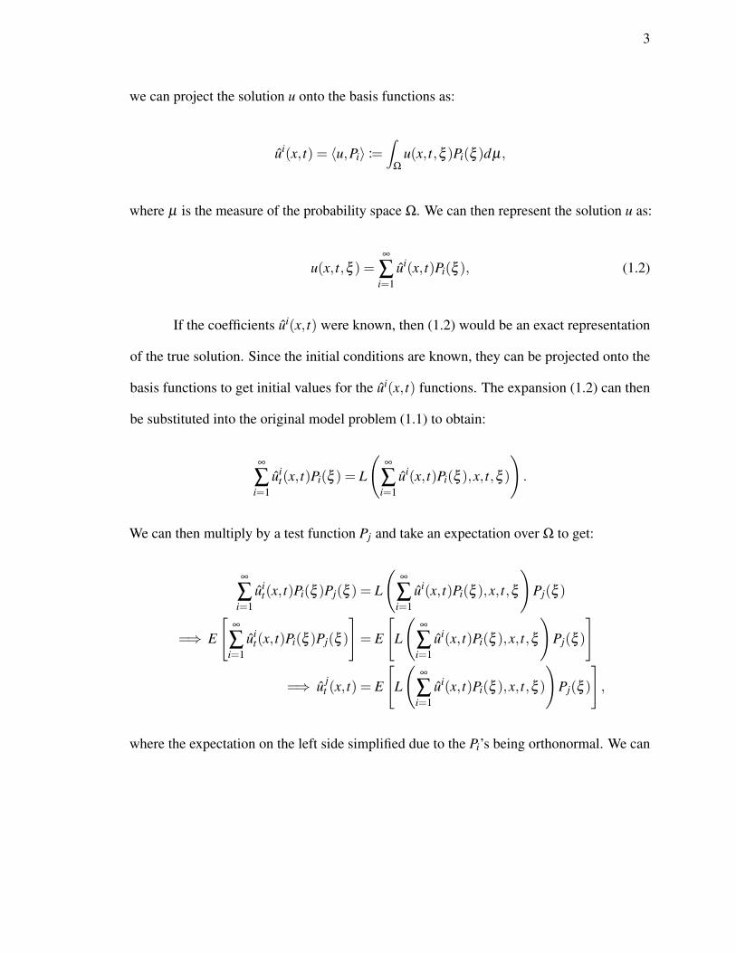
we can project the solution u onto the basis functions as:

ui(x, t) = 〈u,Pi〉 :=∫

Ω

u(x, t,ξ )Pi(ξ )dµ,

where µ is the measure of the probability space Ω. We can then represent the solution u as:

u(x, t,ξ ) =∞

∑i=1

ui(x, t)Pi(ξ ), (1.2)

If the coefficients ui(x, t) were known, then (1.2) would be an exact representation

of the true solution. Since the initial conditions are known, they can be projected onto the

basis functions to get initial values for the ui(x, t) functions. The expansion (1.2) can then

be substituted into the original model problem (1.1) to obtain:

∞

∑i=1

uit(x, t)Pi(ξ ) = L

(∞

∑i=1

ui(x, t)Pi(ξ ),x, t,ξ )

).

We can then multiply by a test function Pj and take an expectation over Ω to get:

∞

∑i=1

uit(x, t)Pi(ξ )Pj(ξ ) = L

(∞

∑i=1

ui(x, t)Pi(ξ ),x, t,ξ

)Pj(ξ )

=⇒ E

[∞

∑i=1

uit(x, t)Pi(ξ )Pj(ξ )

]= E

[L

(∞

∑i=1

ui(x, t)Pi(ξ ),x, t,ξ

)Pj(ξ )

]

=⇒ u jt (x, t) = E

[L

(∞

∑i=1


)Pj(ξ )

],

where the expectation on the left side simplified due to the Pi’s being orthonormal. We can

4

then truncate the infinite expansion on the right hand side at some finite value N, to get:

u jt (x, t) = E

[L

(N

∑i=1


)Pj(ξ )

]1≤ j ≤ N. (1.3)

In practice the right hand side can usually be simplified as well, but it depends on the form

of the differential operator L. This results in a system of coupled deterministic differential

equations for the unknown ui’s. Solving the system will give an approximation of the true

solution u. This is known as the stochastic Galerkin method [26].

A result by Cameron and Martin [6] established that the series (1.2) converges

strongly to L2 functionals, which implies that the series converges for stochastic processes

with finite second moments. The work in [26] coupled the Hermite polynomial expansions

with finite element methods for solving SPDEs, and the method was applied to model

uncertainty in a variety of physical systems [24, 71, 89, 14], and a number of papers were

written on the convergence properties [49, 8, 60, 20] of polynomial chaos methods for

various SPDEs. An extension by Xiu and Karniadakis [88] proposed the use of orthogonal

polynomials in the Askey scheme [1] for a variety of other random variable distributions,

including uniform and beta distributions. The work also established the same strong

convergence results that held for Hermite polynomial expansions of normal random variables.

This method is known as generalized polynomial chaos (gPC), and an overview is provided

in [85]. gPC methods have been applied to a variety of problems in uncertainty quantification,

including problems in fluid dynamics and solid mechanics [87, 90, 91, 66, 15, 45, 42].

Since their introduction, two well-known issues have become apparent with the gPC

method. First, if the number of random variables is too large, then the resulting stochastic

Galerkin system becomes too expensive to solve, and Monte Carlo methods outperform

gPC methods [75, 27]. This is the curse of dimensionality, and in this case is due to the

5

need to introduce multidimensional polynomials, one dimension for each random variable.

Including even modest orders of high dimensional polynomial functions can quickly become

prohibitively expensive. Methods have been proposed to limit the growth rate, including

sparse truncation [29] that selectively eliminates high order polynomials, modifications

of stochastic collocation methods [16], multi-element gPC expansions [75, 76, 21], and

model reduction to project a high dimensional random space onto a lower dimensional one

while still preserving important dynamics [15, 25, 58, 59]. While these methods slow the

curse of dimensionality, none of them entirely eliminate it, and for systems with a high

number of random variables it is more efficient to turn to Monte Carlo methods, which have

a convergence rate independent of the dimension of the random space.

The second issue with the gPC method is that in order to accurately approximate a

solution with unsteady dynamics over a long time interval, a large number of basis functions

must be used (i.e. we must choose a large value for N in equation (1.3)) [27, 53, 29].

This is not particularly surprising, but it is problematic since the amount of work does

not scale linearly with the order of the polynomial basis functions; this issue becomes

particularly troublesome as the number of random variables increases. While multi-element

gPC expansions [75, 76] have been suggested as an option, they do not entirely solve this

issue. Another approach is the time-dependent polynomial chaos method [23, 28], which

integrates for a short period of time, then treats the solution as a new random variable and

attempts to numerically derive an orthogonal polynomial basis for the new random variable.

1.1.2 General Basis

The above results can be extended in a straightforward manner to non-orthonormal

bases as well. Consider any set of functions Ψi∞i=1 that form a basis for L2(Ω), but are not

6

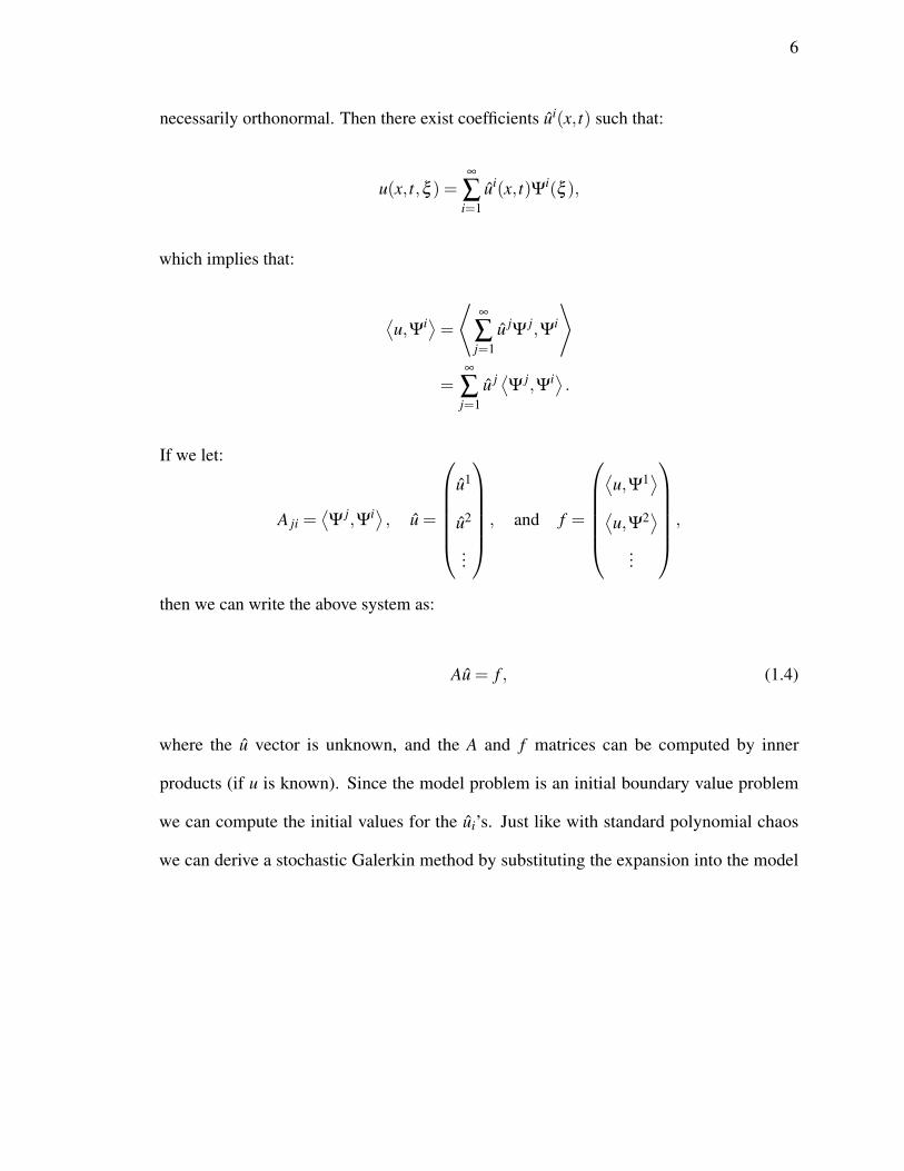
necessarily orthonormal. Then there exist coefficients ui(x, t) such that:

u(x, t,ξ ) =∞

∑i=1

ui(x, t)Ψi(ξ ),

which implies that:

⟨u,Ψi⟩=⟨ ∞

∑j=1

u jΨ

j,Ψi

⟩

=∞

∑j=1

u j ⟨Ψ

j,Ψi⟩ .If we let:

A ji =⟨Ψ

j,Ψi⟩ , u =

u1

u2

...

, and f =

⟨u,Ψ1⟩⟨u,Ψ2⟩

...

,

then we can write the above system as:

Au = f , (1.4)

where the u vector is unknown, and the A and f matrices can be computed by inner

products (if u is known). Since the model problem is an initial boundary value problem

we can compute the initial values for the ui’s. Just like with standard polynomial chaos

we can derive a stochastic Galerkin method by substituting the expansion into the model

7

problem (1.1), multiplying by a test function Ψ j, and taking an expectation over Ω:

∞

∑i=1

uit(x, t)Ψ

i(ξ )Ψ j(ξ ) = L

(∞

∑i=1

ui(x, t)Ψi(ξ ),x, t,ξ

)Ψ

j(ξ )

=⇒ E

[∞

∑i=1

uit(x, t)Ψ

i(ξ )Ψ j(ξ )

]= E

[L

(∞

∑i=1


)Ψ

j(ξ )

].

If we truncate the expansion at finite value N we get:

E

[N

∑i=1

uit(x, t)Ψ

i(ξ )Ψ j(ξ )

]= E

[L

(N

∑i=1


)Ψ

j(ξ )

](1.5)

Now if we let:

A ji =⟨Ψ

j,Ψi⟩ , u =

u1

u2

...

un

, and b j = E

[L

(N

∑i=1


)Ψ

j(ξ )

],

then we get the system

Aut = b, (1.6)

which is a deterministic differential algebraic equation (DAE) whose solution is the values

of the unknown ui coefficients.

8

1.1.3 Conversion Between Bases

Assume we have two distinct bases Ψi∞i=1 and Φi∞

i=1 for L2(Ω), such that:

u(x, t,ξ ) =∞

∑i=1

uiΦ(x, t)Φ

i(ξ ), and

u(x, t,ξ ) =∞

∑i=1

uiΨ(x, t)Ψ

i(ξ ).

Then if we know the values of uiΨ

, we can compute the values of uiΦ

with a standard change

of basis operation:

⟨u,Φ j⟩= ∞

∑i=1

⟨ui

Ψ(x, t)Ψi,Φ j⟩

=∞

∑i=1

uiΨ(x, t)

⟨Ψ

i,Φ j⟩ .Letting

M ji =⟨Ψ

i,Φ j⟩ and b j =⟨u,Φ j⟩

implies that

b = MuΨ. (1.7)

The right hand side is a straightforward computation since uΨ is known, and we can use

equation (1.4) to compute the values of the uΦ coefficients.

The same computation will work when the two bases are finite dimensional instead

of infinite dimensional. If the bases are instead: ΨiNi=1 and ΦiM

i=1, then we can project

9

u(x, t,ξ ) onto the first and second bases:

u(x, t,ξ )≈ uΦ(x, t,ξ ) :=N

∑i=1

uiΦ(x, t)Φ

i(ξ )

u(x, t,ξ )≈ uΨ(x, t,ξ ) :=M

∑i=1

uiΨ(x, t)Ψ

i(ξ ).

If we know the values of the uiΨ

coefficients, then we can compute an approximation of the

uiΦ

coefficients with the same change of basis operation as in the infinite dimensional case:

⟨u,Φ j⟩≈ N

∑i=1

⟨ui

Φ(x, t)Φi(ξ ),Φ j⟩

=N

∑i=1

uiΦ(x, t)

⟨Φ

i(ξ ),Φ j⟩

Letting

M ji =⟨Ψ

i,Φ j⟩ and b j =⟨u,Φ j⟩

implies that

b = MuΨ.

As we know the values of the uΨ coefficients, the right hand side can again be computed and

we may use equation (1.4) to compute an approximation to the values of the uΦ coefficients.

Note that the operations described above first project u onto the subspace spanned by Ψ j,

and then project that projection onto the subspace spanned by Φi.

Chapter 2

Empirical Chaos Expansion

10

11

2.1 Empirical Bases

We now seek to resolve the issue of long-term integration for gPC methods, using

the following general approach.

First, come up with a finite and small set of basis functions that result in a low

projection error over a short time interval (say 0 ≤ t ≤ τ0). Then, perform a stochastic

Galerkin method via equation (1.5) in order to approximate the solution up to time τ . This

will give values for the ui coefficients. Now, come up with a different set of basis functions

that result in a low projection error over the short time interval τ0 ≤ t ≤ τ1. We can use

the previous solution at τ0 as the initial condition, and calculate the initial values of the

ui’s in the new basis by equation (1.7). We can then perform another stochastic Galerkin

method over the new basis to compute the solution up to time τ1. Continuing this process

iteratively will allow us to compute the solution out to a long time t with a low error, and at

each individual step we will only be dealing with a relatively small basis.

The principal issue, then, is determining a subspace spanned by a small number

of basis functions for each interval τi ≤ t ≤ τi+1, such that the solution u will have a low

projection error in the subspace. Once we have such a set of basis functions for each time

interval, then we can follow the approach outlined above to solve the SPDE on a relatively

small set of basis functions.

The work of [23] makes a similar attempt, but relies on integrating the solution to

a small time in the future, and then treating the solution as a new random variable that

must be added to the gPC expansion before integrating out to a later time. This entails

numerically deriving a new set of orthogonal polynomial basis functions that are inferred

from the numerical probability distribution of the solution. In this dissertation we present an

alternate approach, where we no longer require the basis functions to be orthonormal, and

12

instead use techniques of model reduction to construct an empirically optimal set of basis

functions at each given timestep.

2.1.1 Sampling Trajectories

Consider fixing a single point in space x0 and time t0, and then examining how the

function u(x0, t0,ξ ) varies in ξ . This will give a single trajectory of the solution as a function

of the random variable ξ . If we examine many such trajectories then it is reasonable to

assume that a good subspace into which to project the solution should have a low projection

error for most or all of the trajectories.

We can find such trajectories by choosing a set of fixed values for ξ (call them

ξkKk=1), and then solving the resulting deterministic PDE for each ξk, much like Monte

Carlo methods. The difference, however, is that Monte Carlo methods require solving the

PDE for an extremely large number of values of ξ before they converge, and we sample a

much smaller number of trajectories. Once we know the solutions for each of the values of

ξk, we can construct the following matrix, assuming that we have discretized space and

time into the set of points (xi, t j)(M,N)(i, j)=(1,1):

T =

u(x1, t1,ξ1) u(x1, t1,ξ2) . . . u(x1, t1,ξK)

u(x1, t2,ξ1) u(x1, t2,ξ2) . . . u(x1, t2,ξK)

...

u(x1, tN ,ξ1) u(x1, tN ,ξ2) . . . u(x1, tN ,ξK)

u(x2, t1,ξ1) u(x2, t1,ξ2) . . . u(x2, t1,ξK)

...

u(xM, tN ,ξ1) u(xM, tN ,ξ2) . . . u(xM, tN ,ξK).

(2.1)

13

Each row of the matrix T represents a discrete trajectory of the solution as a function

of the random variable ξ . Note that in general this matrix will have far more rows than

columns. We now seek a (hopefully small) set of basis functions in ξ that will result in a

low projection error for each of the rows of T . The motivating assumption is that such a set

of basis functions will also result in a low projection error for the true solution u(x, t,ξ ).

2.1.2 Model Reduction

The field of model reduction focuses primarily on effective methods to solve prob-

lems that exist in very high dimensional spaces by constructing a lower dimensional space,

projecting from the high dimensional space onto the lower dimensional space, and solving

the problem on the lower dimensional space. A key concern is choosing the lower dimen-

sional space in such a way that the important dynamics of the system are retained [56]. A

low dimensional space with a high projection error is useless. One of the classic problems is

to efficiently solve a linear dynamical system that is both observable and controllable [73]:

xt = Ax+Bu

y =Cx,

where x ∈ Rn is a state space vector in a very high dimensional space, A ∈ Rn×Rn is a

constant matrix, B ∈ Rn×Rk is a constant matrix, u ∈ Rk is a control vector whose value

can be changed at different points in time, C ∈ Rm×Rn is a constant matrix, and y is the

observation vector. In many dynamical systems the full state cannot be directly observed,

only part of it, and that is what y represents. The problem cannot be effectively solved due

to the high dimension of the space that the vector x resides in. A standard and well-studied

14

task in the field of model reduction is how to construct a subspace of the state space that x

resides in such that the projection error is low. In this specific case a low projection error

would mean that if we solve the original problem on the lower dimensional subspace with

the same initial conditions and control input, the observed values y would have a small error

compared to the values of y if we computed a solution on the full state space. In the SPDEs

studied in this work the state space is fully observable, so there is no need for the y term.

To frame the problem of constructing an empirical basis in terms of model reduction,

we have to move slightly away from the standard linear dynamical system model. In the

standard model, a trajectory would involve changing values of the x state space vector

through time. In our case, an individual column of the T matrix in the previous section can

be thought of as a single value of the high dimensional state space vector x. Now, however,

instead of varying in time, the state space vector varies as a function of the random variable

ξ .

In principle we could take every row of the T matrix, and treat it as an individual

basis function of the random variable ξ by constructing an interpolating function. But

since the number of rows will, in general, be extremely large, this is not computationally

practical. What we would instead prefer is a small set of vectors such that when we project

any individual row vector from the T matrix onto their span, it has a low projection error.

This is effectively a model reduction problem on a fully observable system.

2.1.3 Proper Orthogonal Decomposition

Proper Orthogonal Decomposition (POD) is a standard tool in the field of model

reduction [7, 37] and is also known as the Karhunen-Loève transform [36, 41], or Principal

Component Analysis [65] in the finite dimensional case. It is often used to construct

15

low dimensional representations of very high dimensional spaces that preserve the most

important dynamics [43, 44, 83].

Following the exposition from [43], in the discrete case we have T in Rn×Rm from

equation 2.1, where we can view each row of T as a sample from a random vector that takes

values in the space Rm. We then seek a set of k < m basis vectors such that the rows of T can

be projected with minimum mean square error onto the k basis vectors. The optimization

problem can be expressed as:

minPk

E[‖v−Pkv‖2

]where v is a random vector from the space sampled by the rows of T , the expectation is over

the rows of T , Pkv is the projection of v onto the optimal choice of k basis vectors, and the

minimization is over all sets of k basis vectors. In practice we can perform a singular value

decomposition of the T matrix in order to compute the POD:

T =UΣV T .

Then the first k columns of the right singular matrix V are the set of k basis vectors that

minimize the mean square error when we project the m rows of the T matrix onto their span.

This will give us a set of k vectors that span a subspace that will result in a low projection

error for all of the rows of the T matrix. We can now construct a basis function in ξ for each

row of the V matrix by constructing an interpolating function through its values at each of

the ξk points.

16

2.1.4 Empirical Chaos Expansion

At this point we can construct a general algorithm to solve the SPDE model prob-

lem (1.1) using successive sets of empirical basis functions. We refer to this method as

empirical chaos expansion. We begin by choosing a set, ξkMk=1, from the range of the

random variable ξ . If there were multiple random variables then we would choose a set of

random vectors from the product space of the random variables. If we wish to solve the

SPDE from time t0 to time t f , then we partition the interval as: t0,τ1,τ2, . . .τn−1, t f . We

then solve the deterministic partial differential equation for each fixed value of ξ in the set

ξkMk=1, starting at time t0 and ending at time τ1. Assuming that the solutions are computed

using a finite difference method, we will then have values for the solution u(x, t,ξ ) at a

set of points (xi, ti,ξk). Fixing a point in space and time then varying the value of ξ , we

get a single row of the matrix T in Section 2.1.1, and we can use the full set of solutions

to construct the full T matrix. We then perform a POD of the T matrix by computing its

singular value decomposition, and choose the first N1 columns of the right singular value

matrix to be the set of basis functions. In practice N1 is chosen so that the N1 +1st singular

value is small relative to the largest singular value. Note that each column of the right

singular value matrix can be viewed as a table of values for the basis function at each of

the ξ values from the set ξk. We could construct an interpolating function for each of

the basis column vectors, though it is computationally faster to simply use the values for a

numerical quadrature formula. We will refer to the set of empirical basis functions generated

for the time interval [t0,τ1] as Ψi1(ξ )

N1i=1, where each Ψi

1 is an individual basis function.

For the first time interval [t0,τ1], we thus approximate the true solution u as:

u(x, t,ξ )≈N

∑i=1

ui(x, t)Ψi1(ξ ).

17

To determine the initial values of the unknown ui coefficients, we project the initial condition

onto each of the basis functions:

ui(x, t0) =⟨u(x, t0),Ψi

1⟩.

The inner product is actually an integral, and since we have a table of values for Ψi1, we can

compute the inner product using numerical quadrature. Once we have the initial values of

the ui coefficients we solve the propagation equation (1.6) for the stochastic Galerkin system

for the SPDE, which computes the values of the ui coefficients up to time τ1. Note that

setting up the system for the propagation equation will require us to compute expectations,

which we can compute using numerical quadrature.

The solution at the final time τ1 can be used as the initial condition to compute

solutions on the interval [τ1,τ2]. We begin by computing the solution to the deterministic

partial differential equation for each fixed value of ξ in the set ξkmk=1, starting at time τ1

and ending at time τ2. We now use the computed solutions to construct a new T matrix

that has trajectories over the time interval [τ1,τ2]. We then perform a POD of the T matrix

by computing its singular value decomposition, and choose the first N2 columns of the

right singular value matrix to be the set of basis functions. This gives a set of empirical

basis functions Ψi2(ξ )

N2i=1. Although we have values ui(x, t) up to time τ1, these are the

coefficients with respect to the old basis Ψi1(ξ ). We can convert them to coefficients

with respect to the new basis Ψi2(ξ ) by following the method described in Section 1.1.3.

Recall that applying the method requires us to compute entries of the matrix:

M ji =⟨

Ψi1,Ψ

j2

⟩.

18

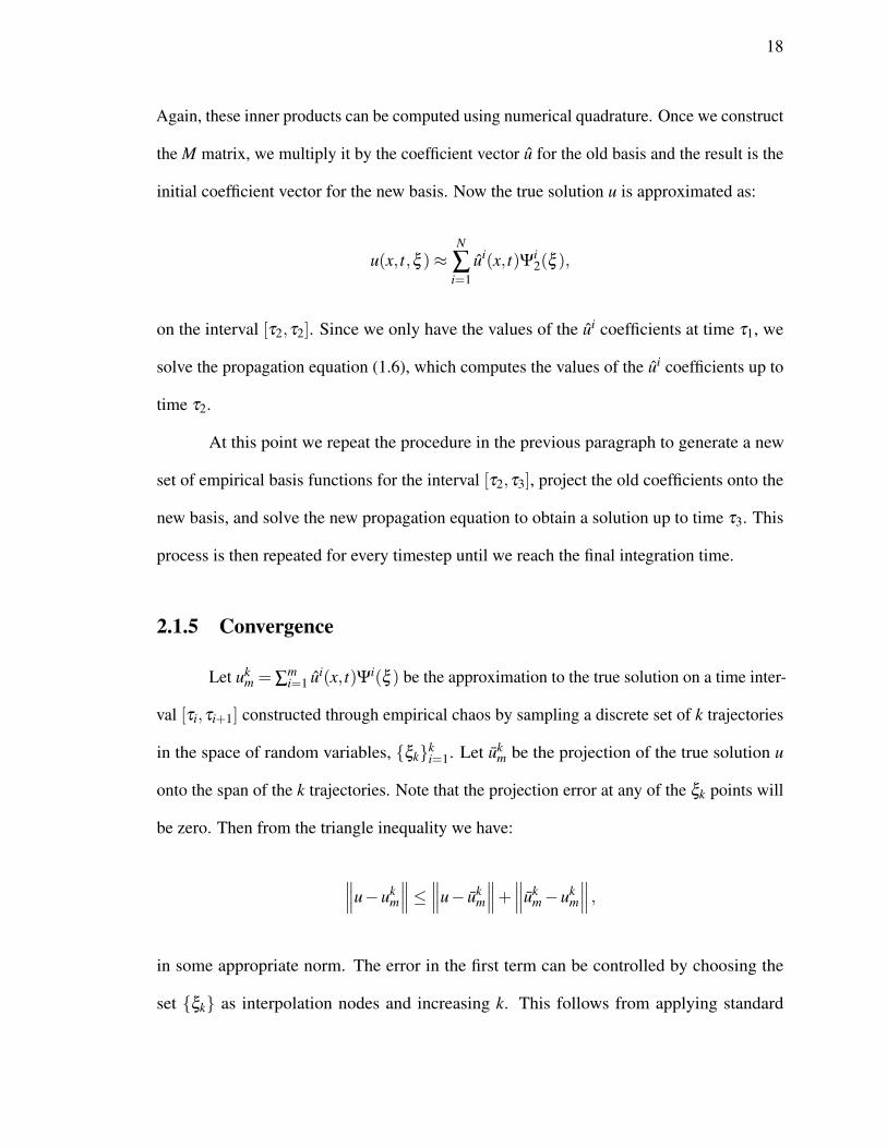
Again, these inner products can be computed using numerical quadrature. Once we construct

the M matrix, we multiply it by the coefficient vector u for the old basis and the result is the

initial coefficient vector for the new basis. Now the true solution u is approximated as:

u(x, t,ξ )≈N

∑i=1

ui(x, t)Ψi2(ξ ),

on the interval [τ2,τ2]. Since we only have the values of the ui coefficients at time τ1, we

solve the propagation equation (1.6), which computes the values of the ui coefficients up to

time τ2.

At this point we repeat the procedure in the previous paragraph to generate a new

set of empirical basis functions for the interval [τ2,τ3], project the old coefficients onto the

new basis, and solve the new propagation equation to obtain a solution up to time τ3. This

process is then repeated for every timestep until we reach the final integration time.

2.1.5 Convergence

Let ukm = ∑

mi=1 ui(x, t)Ψi(ξ ) be the approximation to the true solution on a time inter-

val [τi,τi+1] constructed through empirical chaos by sampling a discrete set of k trajectories

in the space of random variables, ξkki=1. Let uk

m be the projection of the true solution u

onto the span of the k trajectories. Note that the projection error at any of the ξk points will

be zero. Then from the triangle inequality we have:

∥∥∥u−ukm

∥∥∥≤ ∥∥∥u− ukm

∥∥∥+∥∥∥ukm−uk

m

∥∥∥ ,in some appropriate norm. The error in the first term can be controlled by choosing the

set ξk as interpolation nodes and increasing k. This follows from applying standard

19

interpolation theory, assuming sufficient regularity of the solution u. The error in the second

term is due to POD, where instead of projecting u onto the full span of the trajectories,

we project onto a lower dimensional subspace with m basis functions. This error can be

controlled by increasing m.

Computational Cost

In order to fully solve the SPDE at an intermediate timestep i+1 (i.e. any timestep

other than the first), we must perform the following operations:

1. Solve the deterministic PDE for each value of ξ in the set ξkmk=1. If solving a single

instance of the deterministic PDE takes time O(n), then this operation will take time

O(mn). However, it is trivial to parallelize this operation which can dramatically

reduce the computational time.

2. Compute the POD of the T matrix by computing its singular value decomposition.

The T matrix will always have m columns, but the number of rows depends on the

number of finite difference grid points and is almost always much larger than m. Since

we only need the right singular values, which will be an m×m matrix, we can reduce

the cost of the SVD operation by only computing the singular value matrix σ , and the

right singular value matrix V .

3. Project the old ui coefficients onto the new set of basis functions. This operation

requires us to compute the M matrix, which will be Ni+1×Ni (where Ni and Ni+1 are

the number of empirical basis functions for the ith and i+1st timesteps, respectively).

Each entry of the matrix is computed by calculating an inner product with a numerical

quadrature method. We then multiply the M matrix by the old ui coefficient values.

20

4. Compute the left and right hand sides of the propagation equation (1.6). This will

require computing expectations, which can be done with numerical quadrature. The

exact cost of this operation depends on the number of basis functions and also how

complicated the differential operator L is.

5. Solve the propagation equation to advance the solution to the next timestep. Again the

cost of this operation is highly dependent on the differential operator L. In some cases

solving the propagation equation is no harder than solving the deterministic PDE, and

in others it is far more computationally expensive. In either case, it will be a coupled

system of Ni+1 PDEs.

The key advantage of this approach is that we can control the number of empirical basis

functions by adjusting the size of the timestep. gPC uses the same set of basis functions for

every point in time, and for many practical SPDEs this means that achieving accuracy in the

solution out to long integration times requires using a very large set of basis functions. By

constrast, each set of empirical basis functions only needs to have a low projection error

over its corresponding time interval, which can be quite short. This allows the empirical

chaos expansion method to run in linear time as a function of the final integration time, i.e.,

if we want to double the final integration time, it will take about twice as long to compute a

solution using empirical chaos expansion.

Computing Solution Statistics

If there are k total timesteps then we will need to keep track of a set of k sets of basis

functions and their associated coefficients in order to fully reconstruct the solution. In the

end we still have a fully analytic representation of the true solution u, and we can use it

to compute any desired solution statistics. The actual computations will be more complex

21

than those for gPC, due to the fact that the basis functions are not orthogonal, and there are

multiple sets of basis functions (one for each timestep). Let Ψij

N ji=1 be the set of N j basis

functions for timestep j, and let uij

N ji=1 be the corresponding set of coefficients.

If we want to compute the mean of the true solution, then we compute:

E [u(x, t,ξ )] = E

[Nk∗

∑i=1

uik∗Ψ

ik∗

]

=Nk∗

∑i=1

uik∗E[Ψ

ik∗].

where k∗ is the timestep that contains the time t, and E[Ψi

k∗]

can be computed using

numerical quadrature.

If we want to compute the mean square expectation of the true solution, then we

compute:

E [u(x, t,ξ )] = E

(Nk∗

∑i=1

uik∗Ψ

ik∗

)2

= E

[Nk∗

∑i=1

Nk∗

∑j=1

uik∗ u

jk∗Ψ

ik∗Ψ

jk∗

]

=Nk∗

∑i=1

Nk∗

∑j=1

uik∗ u

jk∗E[Ψ

ik∗Ψ

jk∗

]

where k∗ is the timestep that contains the time t, and E[Ψi

k∗Ψjk∗

]can be computed using

numerical quadrature. Other solution statistics can be computed in a similar manner.

22

2.2 One Dimensional Wave Equation

Consider the SPDE:

ut(x, t,ξ ) = ξ ux(x, t,ξ ), 0≤ x≤ 2π, t ≥ 0 (2.2)

u(x,0,ξ ) = cos(x), (2.3)

with periodic boundary conditions, and where ξ is uniformly distributed in [−1,1]. The

exact solution is:

cos(x−ξ t). (2.4)

Note that over the space for this problem:

〈 f ,g〉 :=∫ 1

−1f (ξ )g(ξ )(1/2)dξ

E [ f ] :=∫ 1

−1f (ξ )(1/2)dξ

This hyperbolic SPDE was analyzed in [27], and one of the findings was that for a fixed

polynomial basis, the error will scale linearly with final integration time, thus requiring that

the gPC expansion continually add additional terms in order to achieve accurate long-term

solutions.

2.2.1 Polynomial Chaos Expansion

If we use gPC then we choose the normalized Legendre polynomials to be our basis

functions. Letting Li be the ith normalized Legendre polynomial function, we can perform

23

a stochastic Galerkin method as in Section 1.1.1. The true solution is expanded as:

u(x, t,ξ ) =∞

∑i=1

ui(x, t)Li(ξ ).

Substituting this into Equation 2.2, then multiplying by a test function L j(ξ ), and taking the

expectation of both sides gives:

∞

∑i=1

uit(x, t)L

i(ξ ) = ξ

∞

∑i=1

uix(x, t)L

i(ξ )

=⇒ E

[∞

∑i=1

uit(x, t)L

i(ξ )L j(ξ )

]= E

[ξ

∞

∑i=1

uix(x, t)L

i(ξ )L j(ξ )

]

=⇒∞

∑i=1

uit(x, t)E

[Li(ξ )L j(ξ )

]=

∞

∑i=1

uix(x, t)E

[ξ Li(ξ )L j(ξ )

]=⇒ u j

t =∞

∑i=1

uix(x, t)E

[ξ Li(ξ )L j(ξ )

]

Letting

A ji = E[ξ L jLi

]and u =

u1(x, t)

u2(x, t)

...

simplifies the previous system to:

ut = Aux. (2.5)

Since the initial condition is deterministic, u1(x,0) = cos(x), and ui(x,0) = 0 for i > 1.

We can then truncate the infinite system at some finite value N and solve the resulting

deterministic system of PDEs. To examine the accuracy of the solution we can look at the

mean square expectation at x = 0. The exact value is:

24

E[(u(0, t,ξ )2]= ∫ 1

−1(cos2(ξ t))(1/2)dξ

=12

(1+

cos(t)sin(t)t

). (2.6)

See Figures (2.1, 2.2, 2.3) for a comparison of the exact value of the mean square expectation

with the numerical value computed by applying the stochastic Galerkin method to expansions

truncated at different values of N. It is clear that past a certain point in time all of the PC

expansions diverge from the exact value.

0 5 10 15 20 25 30 35 40 45 50

time

0.1

0.2

0.3

0.4

0.5

0.6

0.7

0.8

0.9

1

N=10

Exact

Figure 2.1: Mean Square Expectation at x = 0 of solution to (2.2), computed usinggPC with stochastic Galerkin using Legendre polynomials up to order 10

25

0 5 10 15 20 25 30 35 40 45 50

time

0.2

0.3

0.4

0.5

0.6

0.7

0.8

0.9

1

N=20

Exact


0 5 10 15 20 25 30 35 40 45 50

time

0.2

0.3

0.4

0.5

0.6

0.7

0.8

0.9

1

N=40

Exact


This is not an issue with the stochastic Galerkin method. In fact, even if we project

the exact solution (2.4) onto the space of Legendre polynomials (see Figure 2.4) and compute

its mean square expectation, we can see that more and more polynomial basis functions are

needed to accurately project the exact solution.

26

This raises another important concern with standard polynomial chaos techniques. If

the initial condition is allowed to be stochastic, then it might be the case that we need a large

number of polynomial functions just to accurately project the initial condition. For example,

if we were to make the initial condition of the problem equal to the exact solution cos(x−ξ t)

for a large value of t, then we would need a large number of Legendre polynomial basis

functions even to accurately compute the solution over a short time interval.

0 5 10 15 20 25 30 35 40 45 50

0

0.1

0.2

0.3

0.4

0.5

0.6

0.7

0.8

0.9

1

N=10

N=20

N=40

Exact

Figure 2.4: Mean Square Expectation x = 0 of the projection of the exact solutionto (2.2) onto gPC basis functions for increasing polynomial order N.


In order to apply an empirical chaos expansion, we must account for the fact that

the basis functions might no longer be orthogonal. This results in the stochastic Galerkin

system becoming slightly more complicated than the one for gPC. If we let Ψi(ξ )Ni=1 be a

set of possibly non-orthogonal basis functions, then we can express the exact solution to

27

Equation (2.2) as:

u(x, t,ξ )≈N

∑i=1

ui(x, t)Ψi(ξ ).

Substituting this expansion into Equation (2.2) results in:

N

∑i=1

uit(x, t)Ψ

i(ξ ) = ξ

N

∑i=1

uix(x, t)Ψ

i(ξ )

We then multiply by a test function Ψ j(ξ ), and take an expectation over Ω of both sides,

resulting in:

N

∑i=1

uit(x, t)Ψ

i(ξ )Ψ j(ξ ) =N

∑i=1

uix(x, t)Ψ

i(ξ )Ψ j(ξ )ξ

=⇒ E

[N

∑i=1

uit(x, t)Ψ

i(ξ )Ψ j(ξ )

]= E

[N

∑i=1

uix(x, t)Ψ

i(ξ )Ψ j(ξ )ξ

]

=⇒N

∑i=1

uit(x, t)E

[Ψ

i(ξ )Ψ j(ξ )]=

N

∑i=1

uix(x, t)E

[Ψ

i(ξ )Ψ j(ξ )ξ]. (2.7)

Letting

M ji = E[Ψ

i(ξ )Ψ j(ξ )], A ji = E

[Ψ

i(ξ )Ψ j(ξ )ξ], and u =

u1(x, t)

u2(x, t)

...

uN(x, t)

,

Equation (2.7) can be expressed as:

Mut = Aux. (2.8)

28

If we know the actual values of the empirical basis functions Ψi and the initial value of the

ui coefficients, then the matrices M and A can both be computed, and the system in (2.8)

can be solved to obtain the values of the coefficients at later times.

We can follow the method in section 2.1 to construct empirical basis functions over

small time intervals by sampling trajectories and applying POD. We begin by choosing a

fixed set of values for the random variable ξ , and solve equation (2.2) for each of the fixed

ξ values, starting at time zero and ending at time τ1. Fixing ξ makes the PDE deterministic,

and it can be solved with any number of existing numerical methods. Here, we use a method

of lines discretization to approximate the spatial derivative and then apply a fourth-order

Runge-Kutta method to perform the time integration (ode45 in Matlab). If we take the

discrete solutions at a fixed point in space and time and vary the value of ξ , then it can

be viewed as a trajectory through the random space. We use these discrete trajectories as

the rows of the T matrix from section 2.1.3, and perform POD by computing the singular

values of T . We then scale the singular values so that the maximum value has magnitude 1,

and cut off the expansion once the magnitude of the corresponding singular values drops

below 10−4. The value of 10−4 is arbitrary and was determined empirically by cutting off

the expansion at varying values. Once the empirical basis functions Ψi(ξ ) have been

generated, we do not explicitly construct an interpolant, but instead use the discrete values

as interpolation nodes for a composite trapezoidal quadrature rule in order to compute

the necessary expectations and inner products. On the first timestep we project the initial

condition u0(x,ξ ) onto the basis functions by computing:

ui(x,0) =⟨u0(x,ξ ),Ψi(ξ )

⟩Ω=∫

Ω

u0(x,ξ )Ψi(ξ )(1/2) dξ .

This gives us the initial values of the ui coefficients. From there, we compute the entries

29

of the M and A matrices in equation (2.8), and solve the system numerically up to the first

timestep, τ1. At that point, we have values for the ui coefficients up to time τ1, and thus

an analytic approximation of the true solution u(x, t,ξ ) up to time τ1. We use the solution

at time τ1 as an initial condition, and then solve the deterministic PDE up to the second

timestep, τ2, for the same fixed set of values for ξ as in the first step. The solutions now

give a set of trajectories in the random space for times between τ1 and τ2. We apply POD to

these trajectories to obtain a new set of basis functions, ΦiMi=1. We then follow the method

in section 1.1.3 to project the coefficients of the solution at time τ1, which are coefficients

for the old basis, Ψi, into coefficients for the new basis, Φi and use them as the initial

values of the ui coefficients. We then use the new basis functions Φi to compute new values

for the M and A matrices from equation (2.8) and solve the DAE up to time τ2.

We now repeat the above process iteratively for times τ2 to τ3, then τ3 to τ4, and

so on, up to the final integration time. In general, choosing smaller timesteps results

in fewer empirical basis functions, while larger timesteps require more empirical basis

functions. Figure 2.5 shows the result of applying this method with a timestep of size 1,

using 120 Chebyshev nodes for values of ξ between−1 and 1 to compute trajectories for the

empirical basis functions. The numerical solution was then used to estimate the mean square

expectation of the true solution at the point x = 0. The maximum number of empirical basis

functions used on any given step was 9.

In order to determine an appropriate number of basis functions to use for a given

timestep, we can examine the singular values from the POD. See figure 2.6, which shows

the singular values for the POD from the first timestep, scaled so that the first singular value

has magnitude 1. There is a sharp drop-off in the magnitude of the singular values around

the fifth singular value. The code for the empirical chaos expansion truncates the expansion

30

0 5 10 15 20 25 30 35 40 45 50

time

0.3

0.4

0.5

0.6

0.7

0.8

0.9

1


Exact

Figure 2.5: Mean Square Expectation at x = 0 of solution to 2.2, computed usingempirical chaos expansion with stochastic Galerkin. Maximum of 9 empirical basisfunctions on each timestep.

once the scaled value of the singular values has dropped below 10−4. Past that point adding

additional basis functions does not appear to increase the accuracy. See figures 2.7 and 2.8,

which show the result of applying the empirical chaos expansion to the one dimensional

wave equation but with only 4 and 5 basis functions, respectively. In both of those cases the

number of empirical basis functions is too low and results in large projection errors. Note

that the cutoff criterion we used results in using 9 basis functions (see figure 2.5).

As mentioned earlier, choosing a larger timestep for the empirical chaos expansion

results in growth of the required number of basis functions for each timestep. This is

unsurprising, since we observe the same behavior with gPC; in order to accurately capture

solution behavior for long time periods, we need more and more basis functions. This

presents an interesting optimization challenge for empirical chaos expansion, since a smaller

basis results in a smaller stochastic Galerkin system, but a smaller timestep means that we

must re-compute more empirical bases. Computing an empirical basis involves sampling

31

1 2 3 4 5 6 7 8 9 10

Singular Value Index

0

0.1

0.2

0.3

0.4

0.5

0.6

0.7

0.8

0.9

1

ScaledMagnitude

Figure 2.6: Singular values from POD for the first timestep when performingempirical chaos expansion to solve (2.2). Singular values are scaled so that themaximum singular value has magnitude 1.

0 5 10 15 20 25 30 35 40 45 50

time

0.3

0.4

0.5

0.6

0.7

0.8

0.9

1


Exact


trajectories of the SPDE, then computing the POD of the trajectories and using it to construct

an empirical basis, and finally projecting the initial condition onto the set of basis functions.

Thus, a smaller timestep reduces the cost of solving the stochastic Galerkin system, but

32

0 5 10 15 20 25 30 35 40 45 50

time

0.3

0.4

0.5

0.6

0.7

0.8

0.9

1


Exact


increases the cost of generating the empirical bases. For the model problem of this section, a

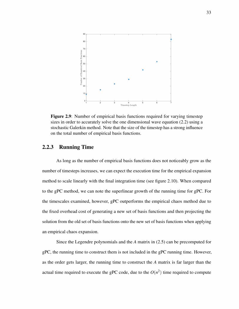
timestep of size 4 appeared to be the optimal choice. Figure 2.9 shows the required number

of basis functions for different choices of timesteps.

33

1 2 3 4 5 6 7

Timestep Length

0

10

20

30

40

50

60

70

80

90

Number

ofEmpiricalBasisFunctions

Figure 2.9: Number of empirical basis functions required for varying timestepsizes in order to accurately solve the one dimensional wave equation (2.2) using astochastic Galerkin method. Note that the size of the timestep has a strong influenceon the total number of empirical basis functions.

2.2.3 Running Time

As long as the number of empirical basis functions does not noticeably grow as the

number of timesteps increases, we can expect the execution time for the empirical expansion

method to scale linearly with the final integration time (see figure 2.10). When compared

to the gPC method, we can note the superlinear growth of the running time for gPC. For

the timescales examined, however, gPC outperforms the empirical chaos method due to

the fixed overhead cost of generating a new set of basis functions and then projecting the

solution from the old set of basis functions onto the new set of basis functions when applying

an empirical chaos expansion.

Since the Legendre polynomials and the A matrix in (2.5) can be precomputed for

gPC, the running time to construct them is not included in the gPC running time. However,

as the order gets larger, the running time to construct the A matrix is far larger than the

actual time required to execute the gPC code, due to the O(n2) time required to compute

34

all of the entries. In the simulations presented, the Legendre polynomials were generated

symbolically and integrated exactly to avoid any error. In order to integrate out to time 200

accurately, we had to use 220 basis functions, and the time required to compute the A matrix

was around 10 hours. In contrast, the empirical chaos method requires no pre-computation

and instead computes its basis functions directly from the sampled trajectories.

20 40 60 80 100 120 140 160 180 200

Final Simulation Time

0

5

10

15

20

25

30

35

Total

RunningTim

e(secon

ds)

Polynomial Chaos

Empirical Chaos

Figure 2.10: Comparison of total running times for solutions of (2.2) computedto the same accuracy using empirical chaos expansion and gPC with stochasticGalerkin.

2.2.4 Basis Function Evolution

Since a new set of basis functions is computed at every timestep in the empirical

expansion, it is natural to examine how they change over time. In order to closely monitor

their evolution, we set the timestep size for the wave equation to 0.1, and examine the values

of the basis functions over time. Figure 2.11 shows the basis function that corresponds to

the largest singular value from POD for the first 5 timesteps (each of size 0.1).

The basis function evolves smoothly over time, although at singular value crossings

35

-1 -0.8 -0.6 -0.4 -0.2 0 0.2 0.4 0.6 0.8 1

ξ

-0.098

-0.096

-0.094

-0.092

-0.09

-0.088

-0.086

Timestep 1

Timestep 2

Timestep 3

Timestep 4

Timestep 5

Figure 2.11: Evolution of the first basis function from POD for the first fivetimesteps in the solution to (2.2) using empirical chaos expansion.

it becomes the function associated with the second largest singular value. Figure 2.12 shows

the magnitudes of the first and second singular values from POD for 100 timesteps, and

there are multiple singular value crossings. Figure 2.13 gives a three dimensional view

of the basis function evolution, where the x-axis is the value of the random variable, and

the y-axis is time. From this figure we can also observe the smooth evolution of this basis

function. In a later chapter we will explore how to take advantage of this smooth evolution.

36

0 10 20 30 40 50 60 70 80 90 100

Timestep

0

50

100

150

200

250

300

First Singular Value

Second Singular Value

Figure 2.12: Evolution of the magnitude of the first two singular values from PODin the solution to (2.2) using empirical chaos expansion.

-0.2

10

8

-0.1

6

Time

4

0

-1

-0.52

ξ

0

0.50

1

0.1

0.2

Figure 2.13: Evolution of the first basis function from POD for the first 100timesteps in the solution to (2.2) using empirical chaos expansion.

37

2.3 Two Dimensional Wave Equation

To illustrate the poor scaling of polynomial chaos methods with multiple variables,

we can consider a slightly modified version of the wave equation (2.2) with two random

variables:

ut(x, t,ξ1,ξ2) = (ξ1ξ2)ux(x, t,ξ ), 0≤ x≤ 2π, t ≥ 0 (2.9)

u(x,0,ξ1,ξ2) = cos(x), (2.10)

with periodic boundary conditions, and where ξ1 and ξ2 are independent and uniformly

distributed in [−1,1]. The exact solution is:

u(x, t,ξ1,ξ2) = cos(x−ξ1ξ2t),


〈 f ,g〉 :=∫ 1

−1

∫ 1

−1f (ξ1,ξ2)g(ξ1,ξ2)(1/4)dξ1dξ2

E [ f ] :=∫ 1

−1

∫ 1

−1f (ξ1,ξ2)(1/4)dξ1dξ2


We may project the solution onto the space of multidimensional Legendre poly-

nomials, which are constructed by taking tensor products of the single variable Legendre

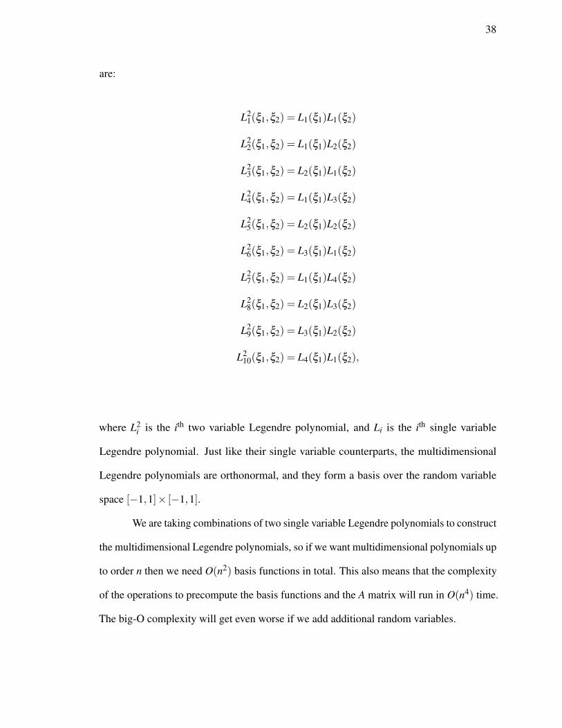
polynomials over each of the two random variables. For example, the first 10 basis functions

38

are:

L21(ξ1,ξ2) = L1(ξ1)L1(ξ2)

L22(ξ1,ξ2) = L1(ξ1)L2(ξ2)

L23(ξ1,ξ2) = L2(ξ1)L1(ξ2)

L24(ξ1,ξ2) = L1(ξ1)L3(ξ2)

L25(ξ1,ξ2) = L2(ξ1)L2(ξ2)

L26(ξ1,ξ2) = L3(ξ1)L1(ξ2)

L27(ξ1,ξ2) = L1(ξ1)L4(ξ2)

L28(ξ1,ξ2) = L2(ξ1)L3(ξ2)

L29(ξ1,ξ2) = L3(ξ1)L2(ξ2)

L210(ξ1,ξ2) = L4(ξ1)L1(ξ2),

where L2i is the ith two variable Legendre polynomial, and Li is the ith single variable

Legendre polynomial. Just like their single variable counterparts, the multidimensional

Legendre polynomials are orthonormal, and they form a basis over the random variable

space [−1,1]× [−1,1].

We are taking combinations of two single variable Legendre polynomials to construct

the multidimensional Legendre polynomials, so if we want multidimensional polynomials up

to order n then we need O(n2) basis functions in total. This also means that the complexity

of the operations to precompute the basis functions and the A matrix will run in O(n4) time.

The big-O complexity will get even worse if we add additional random variables.

39

We can again perform a stochastic Galerkin method as in section 1.1.1 by substituting

the expansion:

u(x, t,ξ1,ξ2) =∞

∑i=1

ui(x, t)L2i (ξ1,ξ2)

into Equation 2.9, then multiplying by a test function L2j , and taking an expectation:

∞

∑i=1

uit(x, t)L

2i (ξ1,ξ2) = ξ1ξ2

∞

∑i=1

uix(x, t)L

2i (ξ1,ξ2)

=⇒ E

[∞

∑i=1

uit(x, t)L

2i (ξ1,ξ2)L2

j(ξ1,ξ2)

]= E

[ξ1ξ2

∞

∑i=1

uix(x, t)L

2i (ξ1,ξ2)L2

j(ξ1,ξ2)

]

=⇒∞

∑i=1

uit(x, t)E

[L2

i (ξ1,ξ2)L2j(ξ1,ξ2)

]=

∞

∑i=1

uix(x, t)E

[ξ1ξ2L2

i (ξ1,ξ2)L2j(ξ1,ξ2)

]=⇒ u j

t (x, t) =∞

∑i=1

uix(x, t)E

[ξ1ξ2L2

i (ξ1,ξ2)L2j(ξ1,ξ2)

](2.11)

Letting

A ji = E[ξ1ξ2L2

jL2i]

and u =

u1(x, t)

u2(x, t)

...

simplifies Equation 2.11 to:

ut = Aux. (2.12)

Since the initial condition is deterministic, u1(x,0) = cos(x), and ui(x,0) = 0 for i > 1.


deterministic system. To examine the solution we can look at the mean square expectation

at x = 0. The exact value is:

40

E[(u(0, t,ξ )2]= ∫ 1

−1

∫ 1

−1(cos2(ξ1ξ2t))(1/2)dξ1dξ2

=12

(1+

Si(2t)2t

). (2.13)

where Si is the sine integral:

Si(z) :=∫ z

0

sin tt

dt.

See figure 2.14 for a comparison of the performance of standard polynomial chaos

as the order increases. For order 40, the number of basis functions is 820. Similar to the one

dimensional wave equation with a single random variable, we need an increasingly higher

order polynomial basis in order to accurately capture the solution out to long time intervals.

Once the matrix A from equation (2.12) has been precomputed, the actual running

time of the polynomial chaos method is fast (though it scales quadratically) for orders up

to 40. However, the current code that we use to generate the Legendre polynomials starts

incurring a prohibitive computational cost at this point, which is why we do not present gPC

results for orders past 40 in the two dimensional case.

41

0 1 2 3 4 5 6 7 8 9 10

Time

0

0.1

0.2

0.3

0.4

0.5

0.6

0.7

0.8

0.9

1

Order = 5

Order = 10

Order = 20

Order = 30

Order = 40

Exact

Figure 2.14: Mean Square Expectation at x = 0 of solution to (2.9), computedusing gPC with stochastic Galerkin using two dimensional Legendre polynomialsof varying order.

2.3.2 Sparse Grid Quadrature

Before we can effectively construct an empirical chaos expansion to solve equation

(2.9), we must first determine an appropriate set of two dimensional random vectors ξimi=1

at which to solve the deterministic version of equation (2.9). In the case where there was a

single random variable we chose Chebyshev nodes on the interval, and determining the value

of the empirical basis functions at those points allowed us to apply numerical quadrature

methods to compute the necessary inner products and expectations. In the two variable case

we have a similar requirement: if we know the values of the empirical basis functions only

at the each of the random vectors in the set ξimi=1, we must be able to apply a numerical

cubature method to compute inner products and expectations involving the basis functions,

or be able to interpolate the basis functions. We could choose to evaluate the solutions on a

uniform two-dimensional grid, but sampling m points in each dimension results in O(m2)

total points. The situation becomes even worse as the total number of random variables

42

grows. To reduce the cost of solving problems on multi-dimensional random spaces, we can

use sparse quadrature methods.

Sparse grid methods were first developed in [70]. While sparse grid methods are

based on tensor product constructions, they avoid taking the full tensor product, and thus

their growth rate scales far slower than the growth rate for full tensor product grids. The

interpolating function is of the form (Lemma 1 from [77]):

Uq = ∑1≤iii, q−d+1≤|iii|≤q

(−1)q−|iii|

d−1

q−|iii|

d⊗k=1

Uik ,

where d is the dimension of the space, q is the level of the sparse grid, the multi-index

iii = (i1, i2, . . . , id), |iii| := ∑dk=1 ik, and Uik is an interpolating function in dimension k over ik

nodes. The condition q−d +1≤ |iii| ≤ q in the summation makes it so that we do not take

the full tensor product.

The construction of sparse grids depends on the choice of interpolating nodes for

each of the Uik . We use Clenshaw-Curtis sparse grids [11], which use extrema of the

Chebyshev polynomials for the interpolation nodes in each individual dimension. A detailed

discussion of their construction and implementation may be found in [19] and [22]. There

are a number of convergence results regarding sparse grid quadrature, and a result from [3]

establishes that for functions on the space

F ld = f : [−1,1]d → R | ∂ iii f continuous, i j ≤ l ∀ 1≤ j ≤ d,

the following error bound holds:

‖ f −UM‖∞≤Cd,lM−l(logM)(l+2)(d−1)+1,

43

where UM is an interpolating polynomial of f on M nodal points, and Cd,l is a constant that

depends on d and l.

For the computations presented in the following sections, we use a sparse grid library

written in Matlab [40, 39].


We can again follow the method in Section 2.1 to construct empirical basis functions

over small time intervals. Since the trajectories are over two random dimensions we use

Clenshaw-Curtis sparse grids to determine at which values of ξ1 and ξ2 we should sample

the solution. See figure 2.15 for a plot of the results. The plot was generated using a grid

depth of 10 (which results in 7196 sampled points) and a timestep size of 1.

0 2 4 6 8 10 12 14 16

time

0.5

0.55

0.6

0.65

0.7

0.75

0.8

0.85

0.9

0.95

1


Exact

Figure 2.15: Mean Square Expectation at x = 0 of solution to (2.9), computedusing empirical chaos expansion with stochastic Galerkin.

44

2.3.4 Running Time

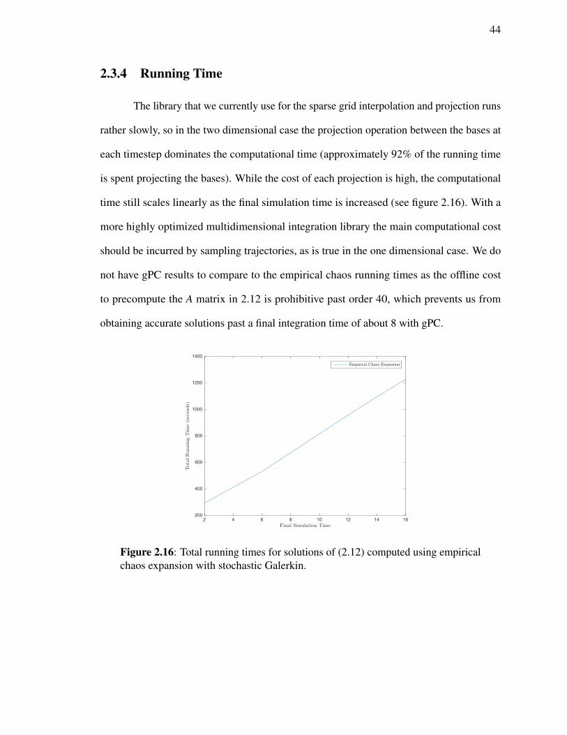
The library that we currently use for the sparse grid interpolation and projection runs

rather slowly, so in the two dimensional case the projection operation between the bases at

each timestep dominates the computational time (approximately 92% of the running time

is spent projecting the bases). While the cost of each projection is high, the computational

time still scales linearly as the final simulation time is increased (see figure 2.16). With a

more highly optimized multidimensional integration library the main computational cost

should be incurred by sampling trajectories, as is true in the one dimensional case. We do

not have gPC results to compare to the empirical chaos running times as the offline cost

to precompute the A matrix in 2.12 is prohibitive past order 40, which prevents us from

obtaining accurate solutions past a final integration time of about 8 with gPC.

2 4 6 8 10 12 14 16


200

400

600

800

1000

1200

1400

Total

RunningTim

e(secon

ds)


Figure 2.16: Total running times for solutions of (2.12) computed using empiricalchaos expansion with stochastic Galerkin.

45

2.4 Diffusion Equation

Consider the SPDE:

ut(x, t,ξ ) = ξ uxx(x, t,ξ ), 0≤ x≤ 6, t ≥ 0 (2.14)

u(x,0,ξ ) = 3I[2,4], (2.15)

with homogeneous Dirichlet boundary conditions, i.e.

u(0, t,ξ ) = u(6, t,ξ ) = 0.

I[a,b] is the indicator function on the interval [a,b] and ξ is a random variable uniformly

distributed on [0,1]. Since the solution to the diffusion equation with these initial conditions

will eventually converge, gPC does quite well. Integrating out to long times accurately does

not require continually increasing the number of basis functions. Even though existing

techniques solve this equation efficiently, it is interesting to examine how the basis functions

for the empirical chaos expansion change over time. The true solution converges to a fixed

value as time goes to infinity, so it is reasonable to expect the empirical basis functions to

converge as well. This turns out to be true, as we will see in the following sections.

Note that over the space of this problem:

〈 f ,g〉 :=∫ 1

0f (ξ )g(ξ )dξ

E [ f ] :=∫ 1

0f (ξ )dξ

46


Since the random variable ξ is uniformly distributed, we again use the Legendre

polynomials Li(ξ )∞i=1 as the set of orthogonal polynomial basis functions. The domain

of the random space is the interval [0,1], so we must use shifted Legendre polynomials,

since the standard Legendre polynomials are orthogonal over the interval [−1,1]. The true

solution can be expressed as:

u(x, t,ξ ) =∞

∑i=1

ui(x, t)Li(ξ ),

and substituting this expression into equation (2.14) gives:

∞

∑i=1

uit(x, t)L

i(ξ ) = ξ

∞

∑i=1

uixx(x, t)L

i(ξ )

Multiplying by a test function L j(ξ ) and taking the expectation gives:

∞

∑i=1

uit(x, t)L

i(ξ )L j(ξ ) = ξ

∞

∑i=1

uixx(x, t)L

i(ξ )L j(ξ )

=⇒ E

[∞

∑i=1

uit(x, t)L

i(ξ )L j(ξ )

]= E

[ξ

∞

∑i=1

uixx(x, t)L

i(ξ )L j(ξ )

]

=⇒∞

∑i=1

uit(x, t)E

[Li(ξ )L j(ξ )

]=

∞

∑i=1

uixx(x, t)E

[ξ Li(ξ )L j(ξ )

]=⇒ u j(x, t) =

∞

∑i=1

uixx(x, t)E

[ξ Li(ξ )L j(ξ )

](2.16)

Letting

A ji = E[ξ Li(ξ )L j(ξ )

]and u =

u1(x, t)

u2(x, t)

...

,

47

equation (2.16) can be simplified to:

ut = Auxx. (2.17)

The infinite system in (2.17) can then be truncated at a finite value N, which results in a

coupled system of N deterministic PDEs. Since the initial condition is deterministic, the

initial values for the ui’s are:

u1(x,0) = 3I[2,4], ui(x,0) = 0 for all i > 1.

Using the initial condition, we can solve the truncated system from equation 2.17, which

gives the evolution of the unknown ui coefficients in time. In figure 2.17 we plot the mean

square expectation of the solution at x = 1, computed using the stochastic Galerkin method

for different polynomial orders. The exact solution was computed by running Monte Carlo

sampling until it converged (∼ 30,000 iterations). The mean square expectation at x = 1

can be computed as:

E[u(1, t,ξ )2]≈ E

( N

∑i=1

ui(x, t)Li(ξ ))

)2=

N

∑i=1

E[(

ui)2].

Unlike the one dimensional wave equation in section 2.2, the solution of which is a travelling

wave, the solutions to the diffusion equation all converge to the same final value. The result

is that polynomial chaos is accurate out to long times even with a small set of basis functions.

Note that in figure 2.17, using 10 polynomial functions captures the solution behavior very

well out to a final time of 100, and using 15 polynomial functions makes the computed

solution almost indistinguishable from the exact solution.

48

0 10 20 30 40 50 60 70 80 90 100

time

0

0.05

0.1

0.15

0.2

0.25

0.3

Exact

N = 10

N = 15

Figure 2.17: Mean Square Expectation at x = 1 of solution to (2.14), computedusing gPC with stochastic Galerkin using Legendre polynomials of varying orderN.


Just as before, we can follow the approach of section 2.1 to construct an empirical

basis and solve the diffusion equation. First, we must analytically derive the stochastic

Galerkin system for an arbitrary basis Ψi(ξ )Ni=1. We approximate the true solution as:

u(x, t,ξ )≈N

∑i=1

ui(x, t)Ψi(ξ ),

where ΨiNi=1 is the set of non-orthogonal empirical basis functions. Substituting this

expansion into equation (2.14) gives:

N

∑i=1

uit(x, t)Ψ

i(ξ ) = ξ

N

∑i=1

uixx(x, t)Ψ

i(ξ )

49

then multiplying by a test function Ψ j and taking the expectation:

N

∑i=1

uit(x, t)Ψ

i(ξ )Ψ j(ξ ) = ξ

N

∑i=1

uixx(x, t)Ψ

i(ξ )Ψ j(ξ )

E

[N

∑i=1

uit(x, t)Ψ

i(ξ )Ψ j(ξ )

]= E

[ξ

N

∑i=1

uixx(x, t)Ψ

i(ξ )Ψ j(ξ )

]N

∑i=1

uit(x, t)E

[Ψ

i(ξ )Ψ j(ξ )]=

N

∑i=1

uixx(x, t)E

[ξ Ψ

i(ξ )Ψ j(ξ )]

(2.18)

Letting

M ji = E[Ψ

i(ξ )Ψ j(ξ )], A ji = E

[ξ Ψ

i(ξ )Ψ j(ξ )], and u =

u1(x, t)

u2(x, t)

...

uN(x, t)

,

simplifies equation (2.18) to:

Mut = Auxx. (2.19)

We can use the solution of (2.19) to compute the values of the unknown ui coefficients at

later times. Just as with the one dimensional wave equation in section 2.2, we begin by

picking a set of values of ξ , this time in the interval [0,1], and solve the diffusion equation

(2.14) from time 0 to time τ1 for each of the values of ξ . In this case we chose the set of

values of ξ to be 200 Chebyshev nodes in the interval [0,1]. Next, we perform POD on

the numerical solutions in order to derive a set of empirical basis functions. Again, we

truncate the basis functions when the corresponding scaled singular value drops below 10−4.

For the first timestep, we project the initial condition onto each empirical basis function by

50

numerically computing:

ui(x,0) =⟨u(x,0,ξ ),Ψi(ξ )

⟩=∫ 1

0u(x,0,ξ )Ψi(ξ )dξ ,

for all i from 1 to N. We then use the empirical basis functions to compute the M and A

matrices in equation (2.18), and solve the system from time 0 to time τ1. However, for

computational efficiency we do not recompute trajectories to find a new empirical basis for

the time interval [τ1, τ2]. Just as with gPC, we can obtain accurate solutions to the diffusion

equation by using a fixed basis. Since we fix the basis, the cost of solving the diffusion

equation is much lower than the cost of solving the one dimensional wave equation, since

we only need to compute trajectories over a short time interval instead of over the entire

integration time.

0 10 20 30 40 50 60 70 80 90 100

time

0

0.05

0.1

0.15

0.2

0.25

0.3

Figure 2.18: Mean square expectation at x = 1 of the solution to the diffusionequation (2.14) computed using an empirical chaos expansion with stochasticGalerkin. The empirical basis functions were generated by solving trajectories upto time t = 1, and then fixing them for the entire integration time. The number ofbasis functions used was 12.

51

2.4.3 Running Time

Figure 2.19 shows a comparison between the total running times of polynomial

chaos and empirical chaos expansion methods when solving the diffusion equation 2.14.

The computational time for the polynomial chaos method scales roughly linearly with the

final simulation time because we can leave the total number of basis functions fixed at 15.

This can be contrasted with the situation for the one dimensional wave equation where we

needed to increase the number of basis functions in order to accurately solve the SPDE out

to longer times. Similarly, the running time for the empirical chaos expansion method also

scales linearly with the final simulation time. For computational efficiency we only compute

the empirical basis functions by sampling trajectories up to time t = 1 and then leave them

fixed for the remaining integration time.

We do not include the cost of pre-computing the A matrix from Equation 2.17 or the

normalized Legendre polynomials in the running time plots. Both methods use roughly the

same number of basis functions. The polynomial chaos expansion uses 15 basis functions

and the empirical chaos expansion uses 12 basis functions. Polynomial chaos slightly

outperforms the empirical chaos expansion due to the cost of generating the set of empirical

basis functions as well as the cost of projecting the initial condition onto the empirical basis

functions. Since the initial condition is deterministic it becomes the coefficient of the first

Legendre polynomial (i.e. L1 = 1) and we do not need to perform any projections when

performing polynomial chaos.

52

0 20 40 60 80 100 120 140 160 180 200


3

3.5

4

4.5

5

5.5

6

Total

RunningTim

e(Secon

ds)

Polynomial Chaos

Empirical Chaos



Even though we do not need to evolve the empirical basis functions to accurately

solve the diffusion equation, we can examine how they change over time if we do re-compute

them at each timestep. For the results in this section we sample trajectories and apply POD

to compute empirical basis functions up to time τ1, but then instead of leaving the basis

fixed, we then use the final solution at time τ1 as an initial condition, and solve the diffusion

equation (2.14) from time τ1 to time τ2 for each value of ξ to compute trajectories. We then

apply a POD to the trajectories to construct a new empirical basis ΦiNi=1. We then take the

final solution at time τ1, which is expressed in terms of coefficients ui corresponding to the

old basis Ψi, and apply the basis transformation from section 1.1.3 to convert them into

coefficients for the new basis Φi. We then use the new basis Φi to recompute the A and

M matrices in equation 2.19, and solve it again to advance the solution up to time τ2. We

then repeat this process iteratively until we have reached the final integration time.

53

Unlike the case for the one dimensional wave, increasing the timestep size does

not have a strong impact on the required number of empirical basis functions. Recall we

decide the number of empirical basis functions by examining the relative magnitudes of the

singular values from POD. As the solution to the diffusion equation converges, we do not

need a growing set of basis functions to accurately capture the solution behavior at later

times. Figure 2.18 shows the computed mean square expectation at x = 1 for an empirical

chaos expansion with timestep size 100. Since the final integration time was also 100, only

one timestep was performed. Even in that case it only used 17 empirical basis functions.

This can be contrasted with the behavior of the one dimensional wave, where a timestep of

size 7 required 83 empirical basis functions.

We set the timestep size to 0.1 in order to closely monitor the evolution of the basis

functions, and integrated out to time 40. Figure 2.21 shows the basis functions for the

first five timesteps for the basis function corresponding to the largest singular value from

POD, and Figure 2.22 shows the basis functions for timesteps 400 and 500. For those

100 timesteps the basis functions only slightly change. The same is also true for the basis

functions associated with the smaller singular values. Figures 2.23 and 2.24 show the

evolution of the basis function associated with the second largest singular value, and this

basis function converges as well.

Figure 2.20 shows how the number of empirical basis functions changes as we

increase the timestep when solving equation (2.14) using an empirical chaos expansion.

Unlike the one dimensional wave equation, the number of basis functions required does not

greatly increase as we increase the size of the timesteps.

54

0 10 20 30 40 50 60 70 80 90 100

Timestep Length

0

2

4

6

8

10

12

14

16

18

20

Number

ofEmpiricalBasisFunctions

Figure 2.20: Number of empirical basis functions required for varying timestepsizes in order to accurately solve the diffusion equation (2.14) using a stochasticGalerkin method. Note that the size of the timestep does not have a strong influenceon the total number of empirical basis functions.

0 0.1 0.2 0.3 0.4 0.5 0.6 0.7 0.8 0.9 1

ξ

-0.085

-0.08

-0.075

-0.07

-0.065

-0.06

Timestep 1

Timestep 2

Timestep 3

Timestep 4

Timestep 5


55

0 0.1 0.2 0.3 0.4 0.5 0.6 0.7 0.8 0.9 1

ξ

-0.25

-0.2

-0.15

-0.1

-0.05

0

Timestep 400

Timestep 500

Figure 2.22: Evolution of the first basis function from POD for timesteps 400 and500 in the solution to (2.14) using empirical chaos expansion.

0 0.1 0.2 0.3 0.4 0.5 0.6 0.7 0.8 0.9 1

ξ

-0.1

-0.05

0

0.05

0.1

0.15

0.2

Timestep 1

Timestep 2

Timestep 3

Timestep 4

Timestep 5

Figure 2.23: Evolution of the second basis function from POD for the first fivetimesteps in the solution to (2.14) using empirical chaos expansion.

56

0 0.1 0.2 0.3 0.4 0.5 0.6 0.7 0.8 0.9 1

ξ

-0.2

-0.1

0

0.1

0.2

0.3

0.4

Timestep 400

Timestep 500

Figure 2.24: Evolution of the second basis function from POD for timesteps 400and 500 in the solution to (2.14) using empirical chaos expansion.

57

Just as with the wave equation, there is a marked drop-off in the magnitudes of

the singular values from POD, which provides a very natural way to automatically choose

the number of empirical basis functions at every timestep (see figure 2.25). Unlike the

wave equation, the largest singular values from POD for the diffusion equation do not seem

to cross, which makes it easier to track the evolution of individual basis functions (see

figure 2.26).

1 2 3 4 5 6 7 8 9 10


0

0.1

0.2

0.3

0.4

0.5

0.6

0.7

0.8

0.9

1

ScaledMagnitude

Figure 2.25: Singular values from POD for timestep 10 when performing empiricalchaos expansion to solve (2.14). Singular values are scaled so that the maximumsingular value has magnitude 1.

58

0 5 10 15 20 25 30 35 40

Time

0

100

200

300

400

500

600

700

800

900



Third Singular Value

Fourth Singular Value

Figure 2.26: Evolution of the magnitude of the first four singular values from PODin the solution to (2.2) using empirical chaos expansion.

59

2.5 Advection-Reaction Equation

In the previous sections, the gPC method outperforms the empirical chaos expansion

even though it uses a far larger polynomial basis for the wave equation. There are two reasons

for this. First, the stochastic Galerkin PDE systems were relatively straightforward to solve,

even when they were high-dimensional. Additionally, the polynomial chaos expansions rely

on pre-computing the A matrix in Equation 2.5 since it always uses the fixed set of Legendre

polynomials as its orthogonal basis. This accounts for much of the efficiency observed in

previous sections.

If we consider the advection-reaction equation:

ut(x, t,ξ ) = ξ ux(x, t,ξ )+ f (x,u),

where the function f (x,u) is nonlinear and not a simple polynomial expression such as u2,

then the resulting stochastic Galerkin system becomes more difficult to evaluate than the

original system, as we will see in subsequent sections. If the order of the polynomial basis

becomes large, then the stochastic Galerkin system for standard polynomial chaos quickly

becomes computationally intractable. In this instance, the benefit of the empirical chaos

expansion becomes evident. Since it limits the number of basis functions to a small number,

the stochastic Galerkin system remains small at each timestep and it remains relatively

inexpensive to solve even when the final integration time is large.

In the subsequent sections we consider the model advection-reaction SPDE:

ut(x, t,ξ ) = ξ ux(x, t,ξ )+0.1 |u|12 , 0≤ x≤ 2π, t ≥ 0 (2.20)

u(x,0,ξ ) = cos(x)+32, (2.21)

60

with periodic boundary conditions and where ξ is uniformly distributed on [−1,1]. Note

that over the space for this problem:

〈 f ,g〉 :=∫ 1

−1f (ξ )g(ξ )(1/2)dξ

E [ f ] :=∫ 1

−1f (ξ )(1/2)dξ

We do not have an analytic solution for this SPDE, so we run Monte Carlo simulations until

they converge in order to check the accuracy of the solutions computed from the polynomial

chaos expansion and the empirical chaos expansion.


If we use gPC then we choose the normalized Legendre polynomials to be our

basis functions. Letting Li be the ith normalized Legendre polynomial, we can perform

a stochastic Galerkin method as in section 1.1.1. The true solution to Equation 2.20 is

expanded as:

u(x, t,ξ ) =∞

∑i=1

ui(x, t)Li(ξ ).

61

Substituting this into equation 2.20, then multiplying by a test function L j(ξ ), and taking

the expectation of both sides gives:

∞

∑i=1

uit(x, t)L

i(ξ ) = ξ

∞

∑i=1

uix(x, t)L

i(ξ )+0.1

∣∣∣∣∣ ∞

∑i=1

uix(x, t)L

i(ξ )

∣∣∣∣∣12

=⇒ E

[∞

∑i=1

uit(x, t)L

i(ξ )L j(ξ )

]= E

[ξ

∞

∑i=1

uix(x, t)L

i(ξ )L j(ξ )

]

+0.1E

∣∣∣∣∣ ∞

∑i=1

uix(x, t)L

i(ξ )

∣∣∣∣∣12

L j(ξ )

=⇒

∞

∑i=1

uit(x, t)E

[Li(ξ )L j(ξ )

]=

∞

∑i=1

uix(x, t)E

[ξ Li(ξ )L j(ξ )

]+0.1E

∣∣∣∣∣ ∞

∑i=1

uix(x, t)L

i(ξ )

∣∣∣∣∣12

L j(ξ )

=⇒ u j

t =∞

∑i=1

uix(x, t)E

[ξ Li(ξ )L j(ξ )

]+0.1E

∣∣∣∣∣ ∞

∑i=1

uix(x, t)L

i(ξ )

∣∣∣∣∣12

L j(ξ )

Letting

A ji = E[ξ L jLi

]f j = 0.1E

∣∣∣∣∣ ∞

∑i=1

uix(x, t)L

i(ξ )

∣∣∣∣∣12

L j(ξ )

u =

u1(x, t)

u2(x, t)

...

62


ut = Aux + f . (2.22)

Since the initial condition is deterministic,

u1(x,0) = cos(x)+32, and ui(x,0) = 0 for i > 1.


deterministic system of PDEs.

The stochastic Galerkin system in equation (2.22) is more difficult to solve than

the original SPDE system in Equation 2.20 due to the nonlinear f term. The expectations

inside cannot be pre-computed since they depend on the values of the ui coefficients at each

point in space and in time. We can compute f at each timestep with numerical quadrature,

but it requires us to compute N expectations, where N is the number of polynomial basis

functions. If we solve the stochastic Galerkin system using a method of lines discretization

or some other finite difference based approach, we will need to compute N expectations for

every timestep of the numerical solver. This becomes very expensive as N grows. In order to

compute the expectations in the f vector we use a composite trapezoidal quadrature method

that uses 300 Chebyshev nodes on the interval [−1,1]. The Legendre polynomials and the A

matrix in equation (2.22) are pre-computed using symbolic arithmetic to avoid any error.

To examine the accuracy of the solution we can look at the mean square expectation

at x = 0, computed from the numerical solution to the stochastic Galerkin system in equa-

tion (2.22). Figures 2.27, 2.28, 2.29, and 2.30 show the numerical gPC results compared

to exact solutions generated by performing 100,000 Monte Carlo iterations. For the short

final time of 10 in figure 2.27, a small number of polynomial basis functions performs well.

63

When integrating out to a final time of 100 in figures 2.28, 2.29, and 2.30, however, a much

higher number of basis functions are required for the solution to be accurate. To numerically

solve the differential equations, we use a method of lines discretization coupled with a fourth

order Runge-Kutta integrator (ode45 in Matlab).

We include results up to polynomial order 40, but for higher orders the stochastic

Galerkin system became unstable. It is not clear at this point whether the instability was due

to the numerical method we used to solve the PDE system, or if the underlying system itself

became unstable for higher polynomial orders.

0 1 2 3 4 5 6 7 8 9 10

time

2

4

6

8

10

12

14

Exact

Polynomial Chaos (N = 5)


Figure 2.27: Mean square expectation x = 0 of solution to (2.20), computed usinggPC with stochastic Galerkin. N is the total number of polynomial basis functionsthat were used. The exact solution was generated by performing Monte Carlosampling with 100,000 realizations.

64

0 10 20 30 40 50 60 70 80 90 100

time

0

200

400

600

800

1000

1200

1400

1600

Exact


Figure 2.28: Mean square expectation x = 0 of solution to (2.20), computed usinggPC with stochastic Galerkin, using Legendre polynomials up to order 10. Theexact solution was generated by performing Monte Carlo sampling with 100,000realizations.

0 10 20 30 40 50 60 70 80 90 100

time

0

200

400

600

800

1000

1200

1400

1600

Exact



65

0 10 20 30 40 50 60 70 80 90 100

time

0

500

1000

1500

Exact



66


If we let Ψi(ξ )Ni=1 be the set of empirical basis functions, we can perform a

stochastic Galerkin method as in section 1.1.1. The true solution to equation (2.20) is

approximated as:

u(x, t,ξ ) =N

∑i=1

ui(x, t)Ψi(ξ ).

Substituting this into equation (2.20), then multiplying by a test function Psi j(ξ ), and taking


N

∑i=1

uit(x, t)Ψ

i(ξ ) = ξ

N

∑i=1

uix(x, t)Ψ

i(ξ )+0.1

∣∣∣∣∣ N

∑i=1

uix(x, t)Ψ

i(ξ )

∣∣∣∣∣12

=⇒ E

[N

∑i=1

uit(x, t)Ψ

i(ξ )Ψ j(ξ )

]= E

[ξ

N

∑i=1

uix(x, t)Ψ

i(ξ )Ψ j(ξ )

]

+0.1E

∣∣∣∣∣ N

∑i=1

uix(x, t)Ψ

i(ξ )

∣∣∣∣∣12

Ψj(ξ )

=⇒

N

∑i=1

uit(x, t)E

[Ψ

i(ξ )Ψ j(ξ )]=

N

∑i=1

uix(x, t)E

[ξ Ψ

i(ξ )Ψ j(ξ )]

+0.1E

∣∣∣∣∣ N

∑i=1

uix(x, t)Ψ

i(ξ )

∣∣∣∣∣12

Ψj(ξ )

67

Letting

A ji = E[ξ Ψ jΨi

]M ji = E

[Ψ jΨi

]f j = 0.1E

∣∣∣∣∣ N

∑i=1

uix(x, t)Ψ

i(ξ )

∣∣∣∣∣12

Ψj(ξ )

u =

u1(x, t)

u2(x, t)

...


Mut = Aux + f . (2.23)

We can follow the method in section 2.1 to construct empirical basis functions over small

time intervals by sampling trajectories and applying POD, and then using those empirical

basis functions to compute the M and A matrices and the f vector in equation (2.23). We

use 300 Chebyshev nodes on the interval [−1,1] as the set of values for ξ . We compute the

intermediate expectations of the f vector using the same composite trapezoidal quadrature

rule that we used for gPC in order to have a fair comparison of the running times. We

also use the same method of lines discretization coupled with a fourth order Runge-Kutta

integrator (ode45 in Matlab) to numerically solve the stochastic Galerkin system.

To examine the accuracy of the solution we look at the mean square expectation at x=

0, computed from the numerical solution to the stochastic Galerkin system in equation (2.23).

Figures 2.31 and 2.32 show the numerical empirical chaos expansion results compared to

68

exact solutions generated by performing 100,000 Monte Carlo iterations. The sampling

points were 300 Chebyshev nodes on the interval [−1,1]

0 1 2 3 4 5 6 7 8 9 10

time

3

4

5

6

7

8

9

10

Exact

Empirical Chaos

Figure 2.31: Mean square expectation at x = 0 of the solution to (2.20) computedusing an empirical chaos expansion with stochastic Galerkin. The timestep sizewas 2, the basis functions were computed by solving the deterministic equation at300 Chebyshev nodes on the interval [−1,1], and the maximum number of basisfunctions used at a single timestep was 33.

Just as in previous sections, we choose the number of empirical basis functions

by examining the magnitude of the scaled singular values from POD. The overall number

needed is higher for this SPDE than the previous ones, but there is still the same marked

drop-off in the magnitude of the scaled singular values. Figure 2.33 shows the magnitude of

the singular values from the POD that was computed at t = 6. There is a marked drop in the

magnitude from the first to the second singular value, and by the sixth singular value the

scaled magnitude has gotten quite small.

The initial mean square expectation fluctuates due to the presence of the advection

term ξ ux, but the reaction term |u|12 dominates the behavior out at long times. This can be

seen when comparing the mean square expectations in Figures 2.31 and 2.32. In Figure 2.31

69

0 10 20 30 40 50 60 70 80 90 100

time

0

500

1000

1500

Exact

Empirical Chaos

Figure 2.32: Mean square expectation at x = 0 of the solution to (2.20) computedusing an empirical chaos expansion with stochastic Galerkin. The timestep sizewas 2, the basis functions were computed by solving the deterministic equation at300 Chebyshev nodes on the interval [−1,1], and the maximum number of basisfunctions used at a single timestep was 33.

0 2 4 6 8 10 12 14 16 18 20


0

0.1

0.2

0.3

0.4

0.5

0.6

0.7

0.8

0.9

1

ScaledMagnitude

Figure 2.33: Singular values from POD for the third timestep when performingempirical chaos expansion to solve (2.20). Singular values are scaled so that themaximum singular value has magnitude 1.

the solution is integrated to final time 10, and there is a noticeable wave-like movement of the

mean square expectation in time. In Figure 2.32, however, the solution is integrated to final

70

time 100, and though the wave-like motion is still present in the mean square expectation,

it has been dominated by the total growth of the solution u due to the reaction term. The

singular values from POD also reflect this behavior. In Figure 2.34, we plot the magnitudes

of the first two singular values that were generated at each timestep of the empirical chaos

expansion solver. As the time grows, the first singular value becomes completely dominant,

which reflects the fact that the reaction term dominates the behavior at later times.

0 10 20 30 40 50 60 70 80 90 100

time

0

0.5

1

1.5

2

2.5

3

3.5

Magnitude

×104



Figure 2.34: Evolution of the magnitude of the first two singular values from PODin the solution to (2.20) using empirical chaos expansion.

2.5.3 Running Time

Since the number of empirical basis functions does not dramatically grow as the

number of timesteps increases, the execution time for the empirical expansion method scales

linearly with the final integration time (see figure 2.10). We can also note the superlinear

growth of the running time for gPC as a function of the final integration time. Although

gPC outperforms the empirical chaos expansion for the smaller integration times, it is

71

outperformed by the empirical chaos expansion for final integration times larger than about

34.

We do not include the cost to pre-compute the A matrix in Equation 2.22, nor the

cost to generate the required the number of Legendre polynomials for the polynomial chaos

expansion. As mentioned previously, however, the entries of the f matrix cannot be pre-

computed, and the computational effort to compute these entries grows as O(N2), where N

is the number of basis functions. As the final simulation time increases, we must increase

the number of polynomial basis functions in order to accurately solve the system, and this

causes the computational cost to grow superlinearly.

10 15 20 25 30 35 40 45 50


0

10

20

30

40

50

60

Total

RunningTim

e(Secon

ds)

Polynomial Chaos

Empirical Chaos



To monitor the evolution of the basis functions, we set the timestep size for the

advection-reaction equation (2.20) to 0.1, and examine the values of the basis functions

72

over time. Figure 2.36 shows the values of the basis function that corresponds to the largest

singular value from POD for the first 5 timesteps (each of size 0.1).

-1 -0.8 -0.6 -0.4 -0.2 0 0.2 0.4 0.6 0.8 1

ξ

-0.0586

-0.0584

-0.0582

-0.058

-0.0578

-0.0576

-0.0574

-0.0572

-0.057

-0.0568

Timestep 1

Timestep 2

Timestep 3

Timestep 4

Timestep 5

Timestep 6


The first basis function evolves smoothly over time, and since there are no crossings

between the first and second singular value, it is straightforward to track the evolution of

this basis function through time. We can also look at the second basis function evolution in

Figures 2.37 and 2.38. The second basis function changes slowly, and thus in Figure 2.37,

which shows the evolution of the second basis function over the first 3 timesteps, the

functions are visually indistinguishable. If we instead look at Figure 2.38, which shows the

evolution of the second basis function over the first 30 timesteps, we can visually observe

its smooth evolution. The first and third singular values have multiple crossings, as we can

see in Figure 2.39, which means that the second basis function will be associated either with

the second or third singular value at different times.

73

-1 -0.8 -0.6 -0.4 -0.2 0 0.2 0.4 0.6 0.8 1

ξ

-0.1

-0.08

-0.06

-0.04

-0.02

0

0.02

0.04

0.06

0.08

0.1

Timestep 1

Timestep 2

Timestep 3

Figure 2.37: Evolution of the second basis function from POD for the first threetimesteps in the solution to (2.20) using empirical chaos expansion.

-1 -0.8 -0.6 -0.4 -0.2 0 0.2 0.4 0.6 0.8 1

ξ

-0.1

-0.08

-0.06

-0.04

-0.02

0

0.02

0.04

0.06

0.08

0.1

Timestep 1

Timestep 10

Timestep 20

Figure 2.38: Evolution of the second basis function from POD for the first 30timesteps in the solution to (2.20) using empirical chaos expansion.

74

0 10 20 30 40 50 60 70 80 90 100

Timestep

0

200

400

600

800

1000

1200

1400

1600

1800

Magnitude



Figure 2.39: Evolution of the magnitude of the second and third singular valuesfrom POD in the solution to (2.20) using empirical chaos expansion.

75

2.6 Reaction-Diffusion Equation

In this section we consider a model reaction-diffusion equation:

ut(x, t,ξ ) = ξ uxx(x, t,ξ )+0.1(

u−|u|32

), 0≤ x≤ 6, t ≥ 0 (2.24)

u(x,0,ξ ) = 3I[2,4], (2.25)

with homogeneous Dirichlet boundary conditions, i.e.

u(0, t,ξ ) = u(6, t,ξ ) = 0.

I[a,b] is the indicator function on the interval [a,b] and ξ is a random variable uniformly

distributed on [0,1]. Since the solution to the reaction-diffusion equation with these initial

conditions will eventually converge, the gPC expansion can achieve high accuracy at long

integration times without needing to include more and more basis functions. Similarly, the

empirical chaos expansion does quite well with the first set of empirical basis functions

that it generates, and does not need to update them by resampling solutions at later times.

However, the inclusion of the nonlinear |u|32 term greatly increases the cost of solving the

stochastic Galerkin system compared to the system generated by the diffusion equation in

Section 2.4.


〈 f ,g〉 :=∫ 1

0f (ξ )g(ξ )dξ

E [ f ] :=∫ 1

0f (ξ )dξ

76

We do not have an analytic solution for this SPDE, so we run Monte Carlo simulations until

they converge in order to check the accuracy of the solutions computed from the polynomial

chaos expansion and the empirical chaos expansion.


If we use gPC then we use normalized Legendre polynomials to be our basis func-

tions. The domain of the random space is the interval [0,1], so we must use shifted Legendre

polynomials, since the standard Legendre polynomials are orthogonal over the interval

[−1,1]. Letting Li be the ith normalized shifted Legendre polynomial, we can perform

a stochastic Galerkin method as in section 1.1.1. The true solution to equation (2.24) is

expanded as:

u(x, t,ξ ) =∞

∑i=1

ui(x, t)Li(ξ ).

77

Substituting this into equation (2.24), then multiplying by a test function L j(ξ ), and taking


∞

∑i=1

uit(x, t)L

i(ξ ) = ξ

∞

∑i=1

uixx(x, t)L

i(ξ )

+0.1

∞

∑i=1

ui(x, t)Li(ξ )−

∣∣∣∣∣ ∞

∑i=1

ui(x, t)Li(ξ )

∣∣∣∣∣32

=⇒ E

[∞

∑i=1

uit(x, t)L

i(ξ )L j(ξ )

]= E

[ξ

∞

∑i=1

uixx(x, t)L

i(ξ )L j(ξ )

]

+0.1E

∞

∑i=1

ui(x, t)Li(ξ )−

∣∣∣∣∣ ∞

∑i=1

ui(x, t)Li(ξ )

∣∣∣∣∣32

L j(ξ )

=⇒

∞

∑i=1

uit(x, t)E

[Li(ξ )L j(ξ )

]=

∞

∑i=1

uix(x, t)E

[ξ Li(ξ )L j(ξ )

]+0.1

(∞

∑i=1

ui(x, t)E[Li(ξ )L j(ξ )

]− E

∣∣∣∣∣ ∞

∑i=1

uix(x, t)L

i(ξ )

∣∣∣∣∣32

L j(ξ )

=⇒ u j

t =∞

∑i=1

uixx(x, t)E

[ξ Li(ξ )L j(ξ )

]+0.1u j−0.1E

∣∣∣∣∣ ∞

∑i=1

uix(x, t)L

i(ξ )

∣∣∣∣∣32

L j(ξ )

78

Letting

A ji = E[ξ L jLi

]f j = 0.1E

∣∣∣∣∣ ∞

∑i=1

uix(x, t)L

i(ξ )

∣∣∣∣∣32

L j(ξ )

u =

u1(x, t)

u2(x, t)

...


ut = Aux + u− f . (2.26)

Since the initial condition is deterministic,

u1(x,0) = 3I[2,4], and ui(x,0) = 0 for i > 1.


deterministic system of PDEs.

The stochastic Galerkin system in equation (2.26) is more difficult to solve than the

original SPDE system in equation (2.24) due to the nonlinear f term. The expectations

inside cannot be pre-computed since they depend on the values of the ui coefficients at each

point in space and in time. We can compute f at each timestep with numerical quadrature,

but it requires us to compute N expectations, where N is the number of polynomial basis

functions. If we solve the stochastic Galerkin system using a method of lines discretization

or some other finite difference based approach, we will need to compute N expectations

79

for every timestep of the numerical solver. In order to compute the expectations in the f

vector we use a composite trapezoidal quadrature method that uses 200 Chebyshev nodes

on the interval [0.001,1]. The Legendre polynomials and the A matrix in equation (2.26) are

pre-computed using symbolic arithmetic to avoid any error. Unlike the reaction-advection

system in section 2.5, however, the solutions to this system will converge, which means

that we do not have to constantly increase the number of polynomial basis functions as we

increase the final integration time.

To solve the original SPDE in equation (2.24) for fixed values of ξ , we use a method

of lines discretization coupled with an multistep implicit ODE solver (ode15s in Matlab).

For the stochastic Galerkin system, however, the nonlinear coupling requires a different

approach to efficiently solve. We implement the IIF2 integrator from [55, 9], which is a

semi-implicit integration technique for nonlinear reaction-diffusion systems. It uses the

method of lines to covert the PDE into a system of ODES, treats the diffusion component

exactly with an exponential integrator, and then treats the reaction component implicitly

to construct a nonlinear system. The nonlinear system is then solved with a fixed point

iteration at each timestep.



tion (2.26). Figures 2.40, 2.41, and 2.42 show the numerical gPC results compared to exact

solutions generated by performing 100,000 Monte Carlo iterations. From the results we can

see that it takes about 10 polynomial basis functions to accurately capture the mean square

expectation out to time 10, and we only need to increase to 15 polynomial basis functions to

accurately capture the mean square expectation out to time 100.

80

0 1 2 3 4 5 6 7 8 9 10

time

0

0.05

0.1

0.15

0.2

0.25

0.3

Exact



Figure 2.40: Mean square expectation x = 1 of solution to (2.24), computed usinggPC with stochastic Galerkin, using Legendre polynomials of varying order N. Theexact solution was generated by performing Monte Carlo sampling with 100,000realizations.

0 10 20 30 40 50 60 70 80 90 100

time

0

0.05

0.1

0.15

0.2

0.25

0.3

Exact


Figure 2.41: Mean square expectation x = 1 of solution to (2.24), computedusing gPC with stochastic Galerkin, using Legendre polynomials of order 5. Theexact solution was generated by performing Monte Carlo sampling with 100,000realizations.

81

0 10 20 30 40 50 60 70 80 90 100

time

0

0.05

0.1

0.15

0.2

0.25

0.3

Exact


Figure 2.42: Mean square expectation x = 1 of solution to (2.24), computedusing gPC with stochastic Galerkin, using Legendre polynomials of order 10. Theexact solution was generated by performing Monte Carlo sampling with 100,000realizations.

82


If we let Ψi(ξ )Ni=1 be the set of empirical basis functions, we can perform a

stochastic Galerkin method as in section 1.1.1. This is essentially the same derivation

as section 2.6.1, except that the Ψi coefficients are not orthogonal. The true solution to

equation (2.24) is approximated as:

u(x, t,ξ ) =N

∑i=1

ui(x, t)Ψi(ξ ).

83

Substituting this into equation (2.24), then multiplying by a test function Ψ j(ξ ), and taking


N

∑i=1

uit(x, t)Ψ

i(ξ ) = ξ

N

∑i=1

uixx(x, t)Ψ

i(ξ )

+0.1

N

∑i=1

ui(x, t)Ψi(ξ )−

∣∣∣∣∣ N

∑i=1

ui(x, t)Ψi(ξ )

∣∣∣∣∣32

=⇒ E

[N

∑i=1

uit(x, t)Ψ

i(ξ )Ψ j(ξ )

]= E

[ξ

N

∑i=1

uix(x, t)Ψ

i(ξ )Ψ j(ξ )

]

+0.1

(E

[N

∑i=1

ui(x, t)Ψ

i(ξ )Ψ j(ξ )

−

∣∣∣∣∣ N

∑i=1

uix(x, t)Ψ

i(ξ )

∣∣∣∣∣32

Ψj(ξ )

=⇒

N

∑i=1

uit(x, t)E

[Ψ

i(ξ )Ψ j(ξ )]=

N

∑i=1

uix(x, t)E

[ξ Ψ

i(ξ )Ψ j(ξ )]

+0.1

(N

∑i=1

ui(x, t)E[Ψ

i(ξ )Ψ j(ξ )]

− E

∣∣∣∣∣ N

∑i=1

uix(x, t)Ψ

i(ξ )

∣∣∣∣∣32

Ψj(ξ )

84

Letting

A ji = E[ξ Ψ jΨi

]M ji = E

[Ψ jΨi

]f j = 0.1E

∣∣∣∣∣ N

∑i=1

uix(x, t)Ψ

i(ξ )

∣∣∣∣∣32

Ψj(ξ )

u =

u1(x, t)

u2(x, t)

...


Mut = Aux +Mu− f . (2.27)

We can follow the method in section 2.1 to construct empirical basis functions by sampling

trajectories and applying POD, and then using those empirical basis functions to compute

the M and A matrices and the f vector in Equation 2.27. We use 200 Chebyshev nodes on

the interval [0.001,1] as the set of values for ξ . We compute the intermediate expectations

of the f vector using the same composite trapezoidal quadrature rule that we used for

standard polynomial chaos in order to have a fair comparison of the running times. To

solve this system we generate the empirical basis functions by sampling the solution over a

small time interval (in this case from t = 0 to t = 1) and we then use those basis functions

without updating them for the entire time interval. This produces accurate solutions since the

reaction-diffusion equation eventually converges, and we do not need to resample trajectories

at later time intervals.

85

To solve the stochastic Galerkin system we use the same IIF2 semi-implicit integrator

described in the previous section [55, 9].



tion (2.27). Figures 2.43 and 2.44 show the numerical empirical chaos expansion results

compared to exact solutions generated by performing 100,000 Monte Carlo iterations. The

sampling points were 200 Chebyshev nodes on the interval [0.001,1].

0 1 2 3 4 5 6 7 8 9 10

time

0

0.05

0.1

0.15

0.2

0.25

0.3

Exact

Empirical Chaos

Figure 2.43: Mean Square Expectation x = 1 of the solution to (2.24) computedusing an empirical chaos expansion with stochastic Galerkin. The timestep of sizewas 2, the basis functions were computed by solving the deterministic equation at200 Chebyshev nodes on the interval [0.001,1], and the number of basis functionswas 12. The exact solution was generated by performing Monte Carlo samplingwith 100,000 realizations.

86

0 10 20 30 40 50 60 70 80 90 100

time

0

0.05

0.1

0.15

0.2

0.25

0.3

Exact

Empirical Chaos

Figure 2.44: Mean Square Expectation x = 1 of the solution to (2.24) computedusing an empirical chaos expansion with stochastic Galerkin. The timestep of sizewas 2, the basis functions were computed by solving the deterministic equation at200 Chebyshev nodes on the interval [0.001,1], and the number of basis functionswas 12. The exact solution was generated by performing Monte Carlo samplingwith 100,000 realizations.

Just as in previous sections, we choose the number of empirical basis functions by

examining the magnitude of the scaled singular values from POD. The difference is that we

do not need to update the basis functions from their initial values by resampling trajectories.

Figure 2.45 shows the magnitude of the singular values from the POD that was computed at

t = 0. There is a marked drop in the magnitude from the first to the second singular value,

and by the sixth singular value the scaled magnitude has gotten quite small.

87

1 2 3 4 5 6 7 8 9 10


0

0.1

0.2

0.3

0.4

0.5

0.6

0.7

0.8

0.9

1

ScaledMagnitude

Figure 2.45: Singular values from POD for the time interval t = 0 to t = 2 whenperforming empirical chaos expansion to solve (2.24). Singular values are scaledso that the maximum singular value has magnitude 1.

2.6.3 Running Time

Since the number of empirical basis functions does not dramatically grow as the

number of timesteps increases, the execution time for the empirical expansion method

scales linearly with the final integration time (see figure 2.46). But since the solution

to the reaction-diffusion equation converges, we also do not need to greatly increase the

number of polynomial basis functions in standard polynomial chaos either, which leads to

its computational time also scaling roughly linearly with the final integration time. The

empirical chaos expansion outperforms standard polynomial chaos towards the end because

it uses a total of 12 basis functions to accurately integrate to time 100, whereas polynomial

chaos needs about 15 basis functions to accurately integrate to time 100.

88

10 20 30 40 50 60 70 80 90 100


0

10

20

30

40

50

60

70

80

Total

RunningTim

e(Secon

ds)

Polynomial Chaos

Empirical Chaos



We do not need to evolve the empirical basis in order to accurately compute the

solution to the reaction-diffusion equation, so as in previous sections we fix the empirical

basis functions to their initial values for computational efficiency. However, we can still

evolve the basis functions and monitor their evolution. We set the timestep size for the

reaction-diffusion equation (2.24) to 0.1, and examine the values of the basis functions over

time. Figure 2.47 shows the values of the basis function that corresponds to the largest

singular value from POD for the first 5 timesteps (each timestep is of size 0.1). The basis

functions smoothly evolve, and in figure 2.48 we see that the empirical basis functions

converge for later timesteps. The evolution of the first three singular values from POD are

plotted in figure 2.49. Similar to the standard diffusion equation there are not any singular

value crossings.

89

0 0.1 0.2 0.3 0.4 0.5 0.6 0.7 0.8 0.9 1

ξ

-0.085

-0.08

-0.075

-0.07

-0.065

-0.06

Timestep 1

Timestep 2

Timestep 3

Timestep 4

Timestep 5


0 0.1 0.2 0.3 0.4 0.5 0.6 0.7 0.8 0.9 1

ξ

-0.16

-0.14

-0.12

-0.1

-0.08

-0.06

-0.04

-0.02

0

Timestep 200

Timestep 250

Timestep 300

Timestep 350

Figure 2.48: Evolution of the first basis function from POD for timesteps 200 to350 in the solution to (2.24) using empirical chaos expansion.

90

0 20 40 60 80 100 120 140 160 180 200

Time

0

100

200

300

400

500

600

700

800




Figure 2.49: Evolution of the magnitude of the first three singular values fromPOD in the solution to (2.24) using empirical chaos expansion.

91

2.7 Acknowledgements

This work was conducted with Professor Melvin Leok at the University of California,

San Diego and is currently being prepared for publication.

Chapter 3

Empirical Basis Evolution Operator

92

93

3.1 Empirical Basis Evolution

The smooth evolution of the empirical basis functions derived from POD suggests

that the empirical basis functions can be computed through an analytic approach that involves

the dynamics of the SPDE. In gPC methods we construct a basis that is orthogonal to the

distribution of the random variables, then project the exact solution onto this basis and

solve for the deterministic coefficients which are functions of space and time. If we wish to

examine how the dynamics of a particular SPDE influence the basis functions for the random

space, we can first take a specific basis–in this case one generated empirically–then project

that basis onto a set of deterministic basis functions that only have a spatial dependence.

After doing so the basis functions of the random variables will have a time dependence and

we will have a DAE whose solution will evolve the basis functions in time.

For the model SPDEs that we analyze, we use the approximation:

u(x, t,ξ )≈N

∑i=1

ui(x)Ψi(ξ , t). (3.1)

The values for Ψi(ξ , t0) will be the values of empirically generated basis functions, and the

values of the ui(x) basis functions will be the values ui(x, t0) of the deterministic coefficients

from the empirical chaos expansion at time t0. In this new approximation the spatial

component is fixed in time, but the random basis functions can vary.

In order to evolve the basis functions in time we can perform a Galerkin method, this

time integrating over the spatial component. We multiply by a test function u j, then integrate

over the spatial domain, R. If we work with the general model problem in Equation 1.1,

94

then this becomes:

N

∑i=1

ui(x)Ψi(ξ , t) = L

(N

∑i=1

ui(x)Ψi(ξ , t),x, t,ξ

)

=⇒N

∑i=1

ui(x)u j(x)Ψi(ξ , t) = L

(N

∑i=1


)u j(x)

=⇒N

∑i=1

∫R

ui(x)u j(x) dxΨi(ξ , t) =

∫R

L

(N

∑i=1


)u j(x) dx. (3.2)

In practice this system can usually be simplified, but it depends on the form of the differential

operator L. This provides a DAE whose solution will evolve the basis functions of the random

variable in time. The general approach we follow is to generate a set of empirical basis

functions over a short time interval using POD, solve the resulting stochastic Galerkin

system, and use the final values of the ui(x, t) coefficients as the fixed spatial basis in (3.2).

We use the empirical basis functions as the initial values of the Ψi(ξ , t) coefficients, and

then solve (3.2) over a short time interval and use the final values of the Ψi(ξ , t) coefficients

as the new empirical basis for the next stochastic Galerkin step.

95

3.1.1 One Dimensional Wave Equation

If we substitute equation (3.1) into equation (2.2) for the one dimensional wave, then

we get:

N

∑i=1

ui(x)Ψit(ξ , t) = ξ

N

∑i=1

uix(x)Ψ

i(ξ , t)

=⇒N

∑i=1

ui(x)u j(x)Ψit(ξ , t) = ξ

N

∑i=1

uix(x)u

j(x)Ψi(ξ , t)

=⇒N

∑i=1

∫ 2π

0ui(x)u j(x) dxΨ

it(ξ , t) = ξ

N

∑i=1

∫ 2π

0ui

x(x)uj(x) dxΨ

i(ξ , t).

Letting

Ψ =

Ψ1

Ψ2

...

ΨN

u =

u1

u2

...

uN

A ji =

∫ 2π

0ui(x)u j(x) dx M ji =

∫ 2π

0ui

x(x)uj(x) dx

implies:

AΨt(ξ , t) = ξ MΨ(ξ , t), (3.3)

which is a DAE whose solution can be used to evolve basis functions in time. The general

approach we use is to first generate a set of empirical basis functions up to a particular time

t∗, using the method of section 2.1. Then the set of empirical basis functions is evolved in

time by solving equation (3.3). In particular, if the matrix A is invertible, then the exact

96

solution to equation (3.3) is:

Ψ(ξ , t) = exp[ξ A−1M(t− t0)

]Ψ(ξ , t0), (3.4)

where exp is the matrix exponential operator. The issue in practice is that A is singular. To

deal with this we can decompose the full system into subsystems where the A matrix is

nonsingular. To accomplish this we can first choose the largest nonsingular square submatrix

of A whose upper left corner is the (1,1) entry of A. If that submatrix has lower right

corner (k,k) where k < n, then we repeat this procedure by constructing another such matrix

whose upper left corner is (k+1,k+1). In practice we calculate the condition number of

the submatrices and use that to determine if the matrix is close to singular. At this point

each subsystem has a nonsingular A matrix, which allows us to directly apply the matrix

exponential operator in equation (3.4) to update the basis functions.

Figure 3.1 shows the result of applying this method to the one-way wave equa-

tion (2.2). The basis functions up to time t = 1 are empirically generated using the standard

method from Section 2.2. For times 1 < t ≤ 10, the empirical basis functions that were gen-

erated at t = 1 are evolved using the exponential operator from Equation 3.4. The numerical

solution closely matches the exact solution up to about t = 4. Past that time the numerical

solution begins to diverge from the exact solution, but still follows the general pattern. For

comparison, we can examine Figure 3.2, where the basis functions are empirically generated

up to time t = 1, and then the basis functions are kept fixed for times 1 < t ≤ 10. When the

basis functions are not evolved at all then the numerical solution matches the exact solution

up to about t = 3, but past that point it wildly diverges from the exact solution, in much the

same way as the standard polynomial chaos expansion.

The basis evolution operator involves computing a matrix exponential, and has the

97

0 1 2 3 4 5 6 7 8 9 10

time

0.3

0.4

0.5

0.6

0.7

0.8

0.9

1


Exact

Figure 3.1: Mean square expectation at x = 0 of solution to (2.2), computed usingempirical chaos expansion with stochastic Galerkin. The basis functions up to timet = 1 are empirically generated. For times 1 < t ≤ 10, the empirical basis functionsthat were generated at t = 1 are evolved using the exponential operator in (3.4).

0 1 2 3 4 5 6 7 8 9 10

time

0.2

0.3

0.4

0.5

0.6

0.7

0.8

0.9

1


Exact

Figure 3.2: Mean square expectation at x = 0 of solution to (2.2), computed usingempirical chaos expansion with stochastic Galerkin. The basis functions up to timet = 1 are empirically generated. For times 1 < t ≤ 10, the basis functions remainfixed at the empirical basis functions that were generated for time t = 1.

potential to be much cheaper to compute than the trajectory sampling approach, and it

suggests the following general strategy:

98

1. Sample a set of trajectories and use POD to generate a set of empirical basis functions

2. Use the exponential basis evolution operator to update the basis functions for a few

additional timesteps without resampling the trajectories

3. Repeat

Although we do not resample the trajectories at each timestep, we need to use smaller

timesteps when applying the matrix exponential operator. In the case of the one dimensional

wave, this results in a slight increase in the running time since the stochastic Galerkin system

is already straightforward to solve. Figure 3.3 shows the result of applying the alternating

timestep strategy, where the first timestep generates empirical basis functions by sampling

trajectories, the second timestep evolves the basis functions using the exponential operator

from 3.4, the third timestep resamples trajectories to generate a new set of empirical basis

functions, the fourth timestep evolves the empirical basis functions using the exponential

operator from 3.4, and so on. We can observe that the solution retains the same accuracy

as when we used trajectory sampling on every timestep. If we do not use the exponential

operator from 3.4 to update the basis functions on alternating timesteps, then the solution

quickly loses accuracy, as we can see in figure 3.4.

99

0 5 10 15 20 25 30 35 40 45 50

Time

0.3

0.4

0.5

0.6

0.7

0.8

0.9

1


Exact

Figure 3.3: Mean square expectation at x = 0 of solution to (2.2), computed usingempirical chaos expansion with stochastic Galerkin with timestep size of 1. Thebasis functions on even timesteps are empirically generated using POD. The basisfunctions on odd timesteps are evolved using the exponential operator in (3.4)

0 5 10 15 20 25 30 35 40 45 50

Time

0.3

0.4

0.5

0.6

0.7

0.8

0.9

1


Exact

Figure 3.4: Mean square expectation at x = 0 of solution to (2.2), computed usingempirical chaos expansion with stochastic Galerkin with timestep size of 1. Thebasis functions on even timesteps are empirically generated using POD. The basisfunctions on odd timesteps are not evolved from their previous values.

100

3.1.2 Diffusion Equation

In section 2.4 we showed that the empirical basis functions for the diffusion equation

do not need to be evolved from their initial values in order to accurately compute the solution.

It is still useful, however, to verify that the empirical basis continues to accurately capture

the solution after we apply the exponential basis evolution operator.

If we substitute equation (3.1) into equation (2.14) for the diffusion equation, then

we get:

N

∑i=1

ui(x)Ψit(ξ , t) = ξ

N

∑i=1

uixx(x)Ψ

i(ξ , t)

=⇒N

∑i=1

ui(x)u j(x)Ψit(ξ , t) = ξ

N

∑i=1

uixx(x)u

j(x)Ψi(ξ , t)

=⇒N

∑i=1

∫ 2π

0ui(x)u j(x) dxΨ

it(ξ , t) = ξ

N

∑i=1

∫ 2π

0ui

xx(x)uj(x) dxΨ

i(ξ , t).

Letting

Ψ =

Ψ1

Ψ2

...

ΨN

u =

u1

u2

...

uN

A ji =

∫ 2π

0ui(x)u j(x) dx M ji =

∫ 2π

0ui

xx(x)uj(x) dx

implies:

AΨt(ξ , t) = ξ AΨ(ξ , t), (3.5)

which is a DAE whose solution can be used to evolve basis functions in time. The general

101

approach we use is to first generate a set of empirical basis functions up to a particular time

t∗, using the method of section 2.1. Then the set of empirical basis functions is evolved in

time by solving equation (3.3). In particular, if the matrix A is invertible, then the exact

solution to equation (3.5) is:

Ψ(ξ , t) = exp[ξ A−1M(t− t0)

]Ψ(ξ , t0), (3.6)

where exp is the matrix exponential operator. Unlike the case with the one dimensional wave

equation, the A matrix in this case is nonsingular and we can directly apply the exponential

operator in equation (3.6) to update the basis functions.

Figure 3.5 shows the result of applying this method to the diffusion equation (2.14).

The basis functions up to time t = 1 are empirically generated using the standard method

from section 2.4. For times 1 < t ≤ 10, the empirical basis functions that were generated

at t = 1 are evolved using the exponential operator from equation (3.6). The numerical

solution closely matches the exact solution. Recall, however, that the empirical basis

functions accurately captured the solution even if they are not evolved at all. We can

examine figure 3.6, where the basis functions are empirically generated up to time t = 1, and

then the basis functions are kept fixed for times 1 < t ≤ 10, which also accurately captures

the solution.

102

0 0.5 1 1.5 2 2.5 3 3.5 4 4.5 5

time

0

0.05

0.1

0.15

0.2

0.25

0.3


Exact

Figure 3.5: Mean square expectation at x = 1 of solution to (2.14), computed usingempirical chaos expansion with stochastic Galerkin. The basis functions up to timet = 1 are empirically generated. For times 1 < t ≤ 10, the basis functions that weregenerated at t = 1 are evolved using the exponential operator in (3.6)

0 0.5 1 1.5 2 2.5 3 3.5 4 4.5 5

time

0

0.05

0.1

0.15

0.2

0.25

0.3


Exact

Figure 3.6: Mean square expectation at x = 1 of solution to (2.14), computed usingempirical chaos expansion with stochastic Galerkin. The basis functions up to timet = 1 are empirically generated. For times 1 < t ≤ 10, the basis functions remainfixed at the empirical basis functions that were generated for time t = 1.

103




Chapter 4

Stochastic Collocation

104

105

In polynomial chaos, we first choose a basis Pi(ξ )Ni=1 for the random space, and

then express the solution to the SPDE as:

u(x, t,ξ )≈N

∑i=1

ui(x, t)Pi(ξ ).

The stochastic Galerkin method presented in previous sections to compute the unknown

ui(x, t) coefficients can prove difficult to apply in practice. One of the principal issues is

that the Galerkin system must be derived analytically, and there are as yet no sufficiently

powerful algorithms to automate this process for fully general problems. Another issue is

that implementing the stochastic Galerkin method usually requires new code to be written in

order to solve the coupled deterministic Galerkin PDE. Finally, in many cases the Galerkin

PDE is significantly more challenging to solve than the original SPDE.

In an attempt to deal with these issues, a class of methods termed nonintrusive

were developed. Nonintrusive methods typically require the original SPDE system to be

solved for fixed values of the random variables and then apply post-processing in order

to compute various moments of the solution distribution. Thus, no new codes need to be

developed beyond a deterministic solver for fixed values of the random variable, and such

codes often already exist. Monte-Carlo methods are an example of a nonintrusive method,

where the solution is computed for fixed values of the random variable, and then moments

of the discrete distribution are used to approximate moments of the continuous distribution

(e.g. the average of the computed solutions is used as an approximation to the mean of the

continuous distribution).

Another commonly used nonintrusive method is stochastic collocation, which was

formalized in [86]. The general approach of stochastic collocation involves choosing a

set of collocation nodes in the random space and picking values for the unknown ui(x, t)

106

coefficients such that the error of the polynomial chaos expansion is zero at the collocation

nodes. This can be accomplished by solving the original SPDE where the random variable

is set to the value of the collocation nodes and/or neighboring nodes, then using those

solutions either for interpolation or numerical integration. In the interpolation approach,

a high order interpolating polynomial is constructed in the random variable space so that

it passes through the computed numerical solutions at all of the collocation points. The

polynomial can then be used to solve for the ui(x, t) coefficients in the polynomial chaos

expansion. In the numerical integration approach (also known as discrete projection or

the pseudospectral approach [84]), the solutions at the collocation nodes are used with

numerical quadrature to evaluate:

ui(x, t) =∫

Ω

u(x, t,ξ )Pi(ξ )dξ ,

for each of the unknown ui(x, t) coefficients.

Another approach, which we use here, is called the Stochastic Response Surface

Method (SRSM) [33, 34] or matrix inversion approach [85]. With this method, we construct

and solve the following system for a set of discrete x and t values:

P1(ξ1) P2(ξ1) . . . PN(ξ1)

P1(ξ2) P2(ξ2) . . . PN(ξ2)

...

P1(ξk) P2(ξk) . . . PN(ξk)

u1(x, t)

u2(x, t)

...

uN(x, t)

=

u(x, t,ξ1)

u(x, t,ξ2)

...

u(x, t,ξk),

(4.1)

where ξiki=1 is the set of collocation points, and the right hand side is the numerical

solution at each of the collocation points. The SRSM has been applied as part of stochastic

107

collocation to solve SPDEs in multiple settings [52, 35, 31, 30, 5], and stochastic collocation

in general is a very active field [2, 57, 18, 50, 17, 67, 72], in no small part due to the relative

ease of implementation relative to stochastic Galerkin.

The system can be constructed so that k = N and there is a unique solution. In

practice, however, we usually create the system so that k >N, causing it to be overdetermined

and then solve it in least squares sense. Just like stochastic Galerkin, SRSM may also be

applied using empirical basis functions generated from POD. The advantage, just as with

SRSM applied to gPC, is that it does not require new code that is specific to a given problem,

beyond code that can solve the problem for a fixed value of the random variable. In the

following sections we show the result of applying SRSM to some model problems using

gPC expansions as well as empirical chaos expansions.

108

4.1 One Dimensional Wave Equation


For the one dimensional wave equation (2.2), we can apply SRSM to the standard

polynomial chaos expansion, choosing the collocation points to be the set of k Chebyshev

nodes on the interval [−1,1]. Each of the k collocation nodes requires one solution to the

original equation, for a fixed value of ξ . These computations can trivially be run in parallel.

After computing the numerical solutions at the collocation nodes we then compute the

least squares solution to the linear system in (4.1) at each fixed value of x and t. The total

computational cost is thus the cost of computing the k solutions of the original system, plus

the cost of inverting a k×N system.

Just like the stochastic Galerkin method, capturing solution behavior for long time

intervals requires N to continually grow. Effectively solving equation (4.1) requires k to be

at least as large as N, so this increases the cost of computing the solution at the collocation

nodes, and also increases the cost of inverting the resulting k×N matrix. Figure 4.1 shows

the result of applying SRSM using gPC for polynomial orders of 10, 20, and 30, and using

the expansions to compute the mean square expectation of the solution at x = 0. Past a

certain point in time all of the numerical solutions diverge from exact value.

109

0 5 10 15 20 25 30 35 40 45 50

time

0

0.1

0.2

0.3

0.4

0.5

0.6

0.7

0.8

0.9

1

Exact

N = 10

N = 20

N = 30

Figure 4.1: Mean Square Expectation at x = 0 of solution to (2.2), computed usinggPC with SRSM using Legendre polynomials of varying order, N. The collocationnodes were chosen to be 600 Chebyshev nodes on the interval [−1,1]


We can apply SRSM to the empirical chaos expansion in a similar way to standard

polynomial chaos. Before solving Equation (4.1), however, we must generate a set of

empirical basis functions. This step also requires solving the original system for a set of

fixed values of ξ , so we may solve the equation for a fixed set once, and then use that set

both for generating the empirical basis and also for estimating the values of the unknown

ui(x, t) coefficients.

We begin by fixing the value of ξ to the collocation points, and solving the deter-

ministic PDE from the starting time up to the first timestep. The solutions are then used to

construct an empirical basis, following the method of Section 2.1. After the basis functions

are generated, we use them to evaluate the left side of equation (4.1). The values of the

solutions are also used to determine the right side of equation (4.1). The system is then

solved to determine the unknown ui(x, t) coefficients. This provides a solution up to the

110

first timestep. The solution at the first timestep is then used as the initial condition, and we

again solve the deterministic PDE at the collocation points from the first timestep to the

second timestep. We use the values of the solutions from timestep one to timestep two to

construct a new set of empirical basis functions, which again lets us evaluate the left side

of equation (4.1). The values of the solutions also provide the right side of equation (4.1).

The system is then solved to determine the unknown ui(x, t) coefficients up to timestep

two. This process is iteratively repeated out to the final timestep, at which point the full

solution is available. Figure 4.2 shows the result of applying SRSM with an empirical chaos

expansion using a timestep of t = 1, using 240 Chebyshev nodes on the interval [−1,1] as

the collocation points, and using the expansion to compute the mean square expectation

of the solution at x = 0. The expansion used at most 9 empirical basis functions for any

given timestep. Similar to stochastic Galerkin, it very faithfully reproduces the behavior of

the mean square expectation of the exact solution while keeping the total number of basis

functions low.

The singular values from POD show a marked drop off, just as in the case of the

stochastic Galerkin method. We use the same singular value cutoff of 10−4 to decide the

total number of empirical basis functions after performing a POD. Figure 4.3 shows the first

ten scaled singular values from POD at the fifth timestep. There is a noticeable drop from

the second to third singular value, and the singular values are very close to zero past the

sixth.

111

0 5 10 15 20 25 30 35 40 45 50

time

0.3

0.4

0.5

0.6

0.7

0.8

0.9

1


Exact

Figure 4.2: Mean square expectation at x = 0 computed using an empirical chaosexpansion with SRSM. The collocation nodes were chosen to be 240 Chebyshevnodes on the interval [−1,1], and the timestep length was t = 1. The maximumnumber of basis functions used on any individual timestep was 9.

1 2 3 4 5 6 7 8 9 10


0

0.1

0.2

0.3

0.4

0.5

0.6

0.7

0.8

0.9

1

ScaledMagnitude

Figure 4.3: Singular values from POD for the first timestep when performingempirical chaos expansion with SRSM to solve (2.2). Singular values are scaled sothat the maximum singular value has magnitude 1.

112

4.1.3 Running Time

We expect the computational time of the empirical chaos expansion with SRSM

to scale linearly as we increase the final time. If the number of basis functions does not

noticeably grow as the final time increases, and the number of collocation points remains

relatively fixed, then the total amount of computational work done at every timestep is

fixed. Thus we expect doubling the final simulation time to result in roughly double the

total amount of computational time. The situation with polynomial chaos is different, since

increasing the number of basis functions also increases the cost of solving the SRSM system.

Figure 4.4 shows a comparison of the running times. Note that the polynomial chaos running

time scales superlinearly with the final time, while the empirical chaos expansion running

time scales linearly with the final running time. The polynomial chaos method used 600

collocation nodes in order to accurately compute the solution, while the empirical chaos

method required 240 collocation nodes.

0 5 10 15 20 25 30 35 40


0

1

2

3

4

5

6

7

8

9

Total

RunningTim

e(Secon

ds)

Polynomial Chaos

Empirical Chaos

Figure 4.4: Comparison of total running times for solutions of (2.2) computed tothe same accuracy using empirical chaos expansion and gPC with SRSM.

113


We now examine how the empirical basis functions evolve between timesteps. We

set the timestep length to 0.1 for this section to closely monitor how the basis functions

change. Figure 4.5 shows how the basis function corresponding to the largest singular value

evolves over the first five timesteps.

-1 -0.8 -0.6 -0.4 -0.2 0 0.2 0.4 0.6 0.8 1

ξ

-0.068

-0.067

-0.066

-0.065

-0.064

-0.063

-0.062

-0.061

Timestep 1

Timestep 2

Timestep 3

Timestep 4

Timestep 5

Figure 4.5: Evolution of the first basis function from POD for the first fivetimesteps in the solution to (2.2) using empirical chaos expansion with SRSM.

This basis function evolves smoothly, but since the first and second singular values

cross multiple times, it can also become the basis function associated with the second

singular value. See Figure 4.6, which shows the magnitudes of the first and second singular

values over 100 timesteps. Figure 4.7 shows a three dimensional view of the evolution of

the first basis function, where time is the third axis.

114

0 10 20 30 40 50 60 70 80 90 100

Timestep

0

50

100

150

200

250

300

350

400



Figure 4.6: Evolution of the magnitude of the first two singular values from PODin the solution to (2.2) using empirical chaos expansion with SRSM.

-0.15

10

-0.1

8

-0.05

6

0

Time

4

0.05

1

2 0.5

ξ

0.1

0

-0.50

0.15

-1

Figure 4.7: Evolution of the first basis function from POD for the first 100timesteps in the solution to (2.2) using empirical chaos expansion with SRSM.

115

4.2 Diffusion Equation


For the diffusion equation (2.14), we can apply SRSM to the gPC expansion, choos-

ing the collocation nodes to be the set of k Chebyshev nodes on the interval [0,1]. Each of

the k collocation points requires one solution to the original equation, for a fixed value of ξ .

Since the solution to the diffusion equation converges, we do not need to dramatically

increase the number of Legendre basis polynomials in order to accurately capture the solution

behavior out to long final integration times. Figure 4.8 shows the result of applying SRSM

using standard polynomial chaos for polynomial orders of 3, 5, and 10, and using the

expansions to compute the mean square expectation of the solution at x = 1. The exact

solution was computed using 75,000 Monte Carlo iterations. All of the computed solutions

follow the general trend of the exact solution, and once we have added 10 polynomial basis,

functions the exact solution is visually indistinguishable from the solution computed using

polynomial chaos.

116

0 5 10 15 20 25 30 35 40 45 50

Time

0

0.05

0.1

0.15

0.2

0.25

0.3

Exact

N = 3

N = 5

N = 10

Figure 4.8: Mean Square Expectation at x = 1 of solution to (2.14), computedusing gPC with SRSM using Legendre polynomials of varying order N. Thecollocation nodes were chosen to be 200 Chebyshev nodes on the interval [0,1].



polynomial chaos. Before solving equation (4.1), however, we must generate a set of




ui(x, t) coefficients. Since the solution to the diffusion equation converges, we can generate

a single set of empirical basis functions by solving the original system up to time 1, and

then using that same set of basis functions for the entire integration time.

Figure 4.9 shows the result of applying SRSM with an empirical chaos expansion

using a timestep of t = 1, with 200 Chebyshev nodes on the interval [0,1] as the collocation

points, and using the expansion to compute the mean square expectation of the solution at

x = 1. The expansion used 12 empirical basis functions. Similar to stochastic Galerkin, it

117

very faithfully reproduces the behavior of the mean square expectation of the exact solution

while keeping the total number of basis functions low.

0 5 10 15 20 25 30 35 40 45 50

Time

0

0.05

0.1

0.15

0.2

0.25

0.3

Exact

Empirical Chaos

Figure 4.9: Mean Square Expectation at x = 1 of solution to (2.14), computedusing empirical chaos expansion with SRSM. The collocation points were chosento be 200 Chebyshev nodes on the interval [0,1], and the timestep length was t = 1.The basis functions were generated by sampling solutions up to the first timestepand then fixing them for the rest of the integration. There were 12 basis functionstotal.



total number of empirical basis functions after performing a POD. Figure 4.10 shows the

first ten scaled singular values from POD at the first timestep. There is a dramatic decay

over the first three singular values, and the singular values are very close to zero past the

fifth.

118

1 2 3 4 5 6 7 8 9 10


0

0.1

0.2

0.3

0.4

0.5

0.6

0.7

0.8

0.9

1

ScaledMagnitude

Figure 4.10: Singular values from POD for first timestep when performing empiri-cal chaos expansion with SRSM to solve (2.14). Singular values are scaled so thatthe maximum singular value has magnitude 1.

4.2.3 Running Time

Since the diffusion equation converges and we can use a fixed basis for both the

polynomial chaos expansion as well as for the empirical chaos expansion, we expect both

methods to perform well. In particular, since we can rely on a fixed number of basis

functions in both methods, both their running times scale linearly with the final integration

time. Figure 4.11 shows a comparison of the running times. The running times for both

methods are nearly identical, since both rely on sampling the solution at 200 fixed values of

ξ , and both use roughly the same number of basis functions (14 for empirical chaos and 15

for polynomial chaos). While the empirical chaos expansion incurs some extra overhead

from performing a singular value decomposition and also performing numerical quadrature,

the cost of the extra operations is insignificant compared to the cost of numerically solving

the original equation for 200 fixed values of ξ and the cost of solving the SRSM system.

119

0 20 40 60 80 100 120 140 160 180 200


1

1.5

2

2.5

3

3.5

4

4.5

5

5.5

6

Total

RunningTim

e(Secon

ds)

Polynomial Chaos

Empirical Chaos

Figure 4.11: Comparison of total running times for solutions of (2.14) computedto the same accuracy using empirical chaos expansion and gPC with SRSM.


We now examine how the empirical basis functions evolve between timesteps. For

the computations in the previous sections we fixed the initial basis and did not evolve it at

all, but for this section we resample the trajectories in order to see how the basis functions

evolve. This is to verify that the basis functions do in fact converge, just as they do when

we solve the diffusion equation using a stochastic Galerkin method. We set the timestep

length to 0.1 for this section to closely monitor how the basis functions change. Figures 4.12

and 4.13 show how the basis functions corresponding to the first two singular values evolve

over the first five timesteps. Figures 4.14 and 4.15 show the basis functions corresponding

to the first two singular values between timesteps 400 and 500. They only slightly change

between those 100 timesteps, indicating that they are converging, just as they did when we

solved the diffusion equation using a stochastic Galerkin method.

We can also track how the magnitudes of the singular values from POD change

between timesteps. Just as is the case with the stochastic Galerkin solution of the diffusion

120

0 0.1 0.2 0.3 0.4 0.5 0.6 0.7 0.8 0.9 1

ξ

-0.085

-0.08

-0.075

-0.07

-0.065

-0.06

Timestep 1

Timestep 2

Timestep 3

Timestep 4

Timestep 5


0 0.1 0.2 0.3 0.4 0.5 0.6 0.7 0.8 0.9 1

ξ

-0.2

-0.15

-0.1

-0.05

0

0.05

0.1

Timestep 1

Timestep 2

Timestep 3

Timestep 4

Timestep 5

Figure 4.13: Evolution of the second basis function from POD for the first fivetimesteps in the solution to (2.14) using empirical chaos expansion with SRSM.

equation, the largest singular values from POD with stochastic collocation do not seem

to cross, which makes it easier to track the evolution of individual basis functions (see

Figure 4.16).

121

0 0.1 0.2 0.3 0.4 0.5 0.6 0.7 0.8 0.9 1

ξ

0

0.05

0.1

0.15

0.2

0.25

Timestep 400

Timestep 500

Figure 4.14: Evolution of the first basis function from POD for timesteps 400 and500 in the solution to (2.14) using empirical chaos expansion with SRSM.

0 0.1 0.2 0.3 0.4 0.5 0.6 0.7 0.8 0.9 1

ξ

-0.2

-0.1

0

0.1

0.2

0.3

0.4

Timestep 400

Timestep 500

Figure 4.15: Evolution of the second basis function from POD for timesteps 400and 500 in the solution to (2.14) using empirical chaos expansion with SRSM.

122

0 50 100 150 200 250 300 350 400 450 500

Timestep

0

100

200

300

400

500

600

700

800

900




Figure 4.16: Evolution of the magnitude of the first three singular values fromPOD in the solution to (2.2) using empirical chaos expansion.

123

4.3 Advection-Reaction Equation


For the advection-reaction equation (2.20), we can apply SRSM to the standard

polynomial chaos expansion, choosing the collocation points to be the set of k Chebyshev

nodes on the interval [−1,1]. Each of the k collocation points requires one solution to the

original equation, for a fixed value of ξ . These computations can trivially be run in parallel.

After computing the numerical solutions at the collocation points we then compute the

least squares solution to the linear system in (4.1) at each fixed value of x and t. The total

computational cost is thus the cost of computing the k solutions of the original system, plus

the cost of inverting a k×N system.

Just as with the stochastic Galerkin method, capturing solution behavior for long

time intervals requires N to continually grow. Effectively solving (4.1) requires k to be at

least as large as N, so this increases the cost of computing the solution at the collocation

points, and also increases the cost of inverting the resulting k×N matrix. Figure 4.17 shows

the result of applying SRSM using standard polynomial chaos for polynomial orders of 5

and 10 and using the expansions to compute the mean square expectation of the solution at

x = 0. Past a certain point in time all of the numerical solutions diverge from exact value.

124

0 1 2 3 4 5 6 7 8 9 10

Time

3

4

5

6

7

8

9

10

Exact

N = 5

N = 10

Figure 4.17: Mean square expectation x = 0 of solution to (2.20), computed usinggPC with SRSM. N is the total number of polynomial basis functions that wereused. The collocation points were chosen to be 240 Chebyshev nodes on theinterval [−1,1].



polynomial chaos. Before solving equation (4.1), however, we must generate a set of




ui(x, t) coefficients.

We begin by fixing the value of ξ to the collocation points, and solving the deter-

ministic PDE from the starting time up to the first timestep. The solutions are then used to

construct an empirical basis, following the method of section 2.1. After the basis functions

are generated, we use them to evaluate the left side of equation (4.1). The values of the

solutions are also used to determine the right side of (4.1). The system is then solved to

determine the unknown ui(x, t) coefficients. This provides a solution up to the first timestep.

125

The solution at the first timestep is then used as the initial condition, and we again solve the

deterministic PDE at the collocation points from the first timestep to the second timestep.

We use the values of the solutions from timestep one to timestep two to construct a new

set of empirical basis functions, which again lets us evaluate the left side of equation (4.1).

The values of the solutions also provide the right side of (4.1). The system is then solved to

determine the unknown ui(x, t) coefficients up to timestep two. This process is iteratively

repeated out to the final timestep, at which point the full solution is available. Figure 4.18

shows the result of applying SRSM with an empirical chaos expansion using a timestep

of t = 1, using 240 Chebyshev nodes on the interval [−1,1] as the collocation points, and

using the expansion to compute the mean square expectation of the solution at x = 0. The

expansion used at most 22 empirical basis functions for any given timestep. Similar to

stochastic Galerkin, it very faithfully reproduces the behavior of the mean square expectation

of the exact solution while keeping the total number of basis functions low.

0 5 10 15 20 25 30 35 40 45 50

Time

0

20

40

60

80

100

120

140

160

180

200

Exact

Empirical Chaos

Figure 4.18: Mean square expectation at x = 0 of the solution to (2.20) computedusing an empirical chaos expansion with SRSM with a timestep size of 1. Thecollocation points were chosen to be 240 Chebyshev nodes on the interval [−1,1].The maximum number of basis functions used on any individual timestep was 22.

126




first ten scaled singular values from POD at the fifth timestep. There is a noticeable drop

from the second to third singular value, and the singular values are very close to zero past

the sixth.

1 2 3 4 5 6 7 8 9 10


0

0.1

0.2

0.3

0.4

0.5

0.6

0.7

0.8

0.9

1

ScaledMagnitude

Figure 4.19: Singular values from POD for the fifth timestep when performingempirical chaos expansion to solve (2.20). Singular values are scaled so that themaximum singular value has magnitude 1.

4.3.3 Running Time

We expect the computational time of the empirical chaos expansion with SRSM

to scale linearly as we increase the final time. If the number of basis functions does not

noticeably grow as the final time increases, and the number of collocation points remains

relatively fixed, then the total amount of computational work done at every timestep is

fixed. Thus we expect doubling the final simulation time to result in roughly double the

127

total amount of computational time. The situation with polynomial chaos is different, since

increasing the number of basis functions also increases the cost of solving the SRSM system.

We also need to steadily increase the number of collocation nodes for polynomial chaos as

the final integration time increases. Figure 4.20 shows a comparison of the running times.

Note that the polynomial chaos running time scales superlinearly with the final time, while

the empirical chaos expansion running time scales linearly with the final running time. The

polynomial chaos method used 800 collocation nodes for the final time in order to accurately

compute the solution, while the empirical chaos method requires 200 collocation nodes.

10 15 20 25 30 35 40 45 50 55 60


0

5

10

15

20

25

Total

RunningTim

e(Secon

ds)

Polynomial Chaos

Empirical Chaos



We now examine how the empirical basis functions evolve between timesteps. We

set the timestep length to 0.1 for this section to closely monitor how the basis functions

change. Figure 4.21 shows how the basis function corresponding to the largest singular

value evolves over the first five timesteps. Figure 4.22 shows the evolution of the magnitudes

128

of the first, second, and third singular values over 100 timesteps.

-1 -0.8 -0.6 -0.4 -0.2 0 0.2 0.4 0.6 0.8 1

ξ

-0.0652

-0.065

-0.0648

-0.0646

-0.0644

-0.0642

-0.064

-0.0638

Timestep 1

Timestep 2

Timestep 3

Timestep 4

Timestep 5


0 10 20 30 40 50 60 70 80 90 100

Timestep

0

200

400

600

800

1000

1200

1400

1600

1800




Figure 4.22: Evolution of the magnitude of the first, second, and third singularvalues from POD in the solution to (2.20) using empirical chaos expansion withSRSM.

129

4.4 Reaction-Diffusion Equation


For the reaction-diffusion equation (2.24), we can apply SRSM to the gPC expansion,

choosing the collocation points to be the set of k Chebyshev nodes on the interval [0,1].

Each of the k collocation points requires one solution to the original equation, for a fixed

value of ξ .

Since the solution to the diffusion equation converges, we do not need to dramatically

increase the number of Legendre basis polynomials in order to accurately capture the solution

behavior out to long final integration times. Figure 4.23 shows the result of applying SRSM

using gPC for polynomial orders of 4 and 10, and using the expansions to compute the

mean square expectation of the solution at x = 1. The exact solution was computed using

100,000 Monte Carlo iterations. All of the computed solutions follow the general trend of

the exact solution, and once we have added 10 polynomial basis functions the exact solution

is visually indistinguishable from the solution computed using polynomial chaos.

130

0 5 10 15 20 25 30 35 40 45 50

Time

0

0.05

0.1

0.15

0.2

0.25

0.3

Exact

N = 4

N = 10

Figure 4.23: Mean square expectation x = 1 of solution to (2.24), computed usinggPC with SRSM, using Legendre polynomials of varying order N. The collocationpoints were chosen to be 300 Chebyshev nodes on the interval [0.00001,1]



polynomial chaos. Before solving (4.1), however, we must generate a set of empirical basis

functions. This step also requires solving the original system for a set of fixed values of ξ , so

we may solve the equation for a fixed set once, and then use that set both for generating the

empirical basis and also for estimating the values of the unknown ui(x, t) coefficients. Since

the solution to the diffusion equation converges, we can generate a single set of empirical

basis functions by solving the original system up to time 1, and then using that same set of

basis functions for the entire integration time.

Figure 4.24 shows the result of applying SRSM with an empirical chaos expansion

using a timestep of t = 2, with 300 Chebyshev nodes on the interval [0.01,1] as the colloca-

tion points, and using the expansion to compute the mean square expectation of the solution

at x = 1. The expansion used 14 empirical basis functions. Similar to stochastic Galerkin, it

131

very faithfully reproduces the behavior of the mean square expectation of the exact solution

while keeping the total number of basis functions low.

0 5 10 15 20 25 30 35 40 45 50

Time

0

0.05

0.1

0.15

0.2

0.25

0.3

Exact

Empirical Chaos

Figure 4.24: Mean square expectation at x = 1 of the solution to (2.24) computedusing an empirical chaos expansion with SRSM. The collocation points werechosen to be 300 Chebyshev nodes on the interval [0.01,1], and the timestep lengthwas t = 2. The basis functions were generated by sampling solutions up to the firsttimestep and then fixing them for the rest of the integration. There were 14 basisfunctions total.




first ten scaled singular values from POD at the first timestep. There is a dramatic decay

over the first three singular values, and the singular values are very close to zero past the

eighth.

132

1 2 3 4 5 6 7 8 9 10


0

0.1

0.2

0.3

0.4

0.5

0.6

0.7

0.8

0.9

1

ScaledMagnitude

Figure 4.25: Singular values from POD for the time interval t = 0 to t = 2 whenperforming empirical chaos expansion to solve (2.24). Singular values are scaledso that the maximum singular value has magnitude 1.

4.4.3 Running Time

Since the solution to the reaction-diffusion equation converges and we can use a

fixed basis for both the polynomial chaos expansion as well as for the empirical chaos

expansion, we expect both methods to perform well. In particular, since we can rely on a

fixed number of basis functions in both methods, both their running times scale linearly

with the final integration time. Figure 4.26 shows a comparison of the running times. The

running times for both methods are nearly identical, since both rely on sampling the solution

at 300 fixed values of ξ , and both use roughly the same number of basis functions (14 for

empirical chaos and 15 for polynomial chaos). While the empirical chaos expansion incurs

some extra overhead from performing a singular value decomposition and also performing

numerical quadrature, the cost of the extra operations is insignificant compared to the cost

of numerically solving the original equation for 300 fixed values of ξ and the cost of solving

the SRSM system.

133

20 40 60 80 100 120 140 160


2

3

4

5

6

7

8

9

Total

RunningTim

e(Secon

ds)

Polynomial Chaos

Empirical Chaos



We now examine how the empirical basis functions evolve between timesteps. For

the computations in the previous sections we fixed the initial basis and did not evolve it at

all, but for this section we resample the trajectories in order to see how the basis functions

evolve. This is to verify that the basis functions do in fact converge, just as they do when

we solve the diffusion equation using a stochastic Galerkin method. We set the timestep

length to 0.1 for this section to closely monitor how the basis functions change. Figure 4.27

shows how the basis function corresponding to the first singular value evolves over the

first five timesteps. Figure 4.28 shows the basis function corresponding to the first singular

value between timesteps 400 and 500. There is only a slight change between those 100

timesteps, indicating that the basis function is converging, just as it did when we solved the

reaction-diffusion equation using a stochastic Galerkin method.

We can also track how the magnitudes of the singular values from POD change

between timesteps. Just as is the case with the stochastic Galerkin solution of the reaction-

134

0 0.1 0.2 0.3 0.4 0.5 0.6 0.7 0.8 0.9 1

ξ

-0.068

-0.066

-0.064

-0.062

-0.06

-0.058

-0.056

-0.054

-0.052

-0.05

Timestep 1

Timestep 2

Timestep 3

Timestep 4

Timestep 5


0 0.1 0.2 0.3 0.4 0.5 0.6 0.7 0.8 0.9 1

-0.14

-0.12

-0.1

-0.08

-0.06

-0.04

-0.02

0

Timestep 400

Timestep 500

Figure 4.28: Evolution of the first basis function from POD for timesteps 400 to500 in the solution to (2.24) using empirical chaos expansion.

diffusion equation, the largest singular values from POD with stochastic collocation do not

seem to cross, which makes it easier to track the evolution of individual basis functions (see

figure 4.29).

135

0 20 40 60 80 100 120 140 160 180 200

Timestep

0

100

200

300

400

500

600

700

800

900

1000




Figure 4.29: Evolution of the magnitude of the first three singular values fromPOD in the solution to (2.24) using empirical chaos expansion with SRSM.

136




Chapter 5

Conclusion

137

138

5.1 Future Work

Since their inception, polynomial chaos techniques have been successfully applied

to a number of numerical problems that arise in uncertainty quantification. This work

introduces a method to generate a set of empirical basis functions that varies with time to

take the place of the standard orthogonal polynomial basis that remains fixed for the entire

integration time. We demonstrate its numerical accuracy and efficiency over long-term

integrations with multiple model problems. We also introduce a method to numerically

evolve the empirical basis functions without needing to resample solutions of the original

SPDE. We demonstrate that the running time of the empirical chaos method scales linearly

with the final integration time. Thus, it has the potential to address one of the two principal

issues with applying polynomial chaos techniques–solving problems out to long-term

integrations is often inefficient due to the need to continually increase the number of

polynomial basis functions.

This work does not, however, present a solution to the second and most fundamental

issue–the curse of dimensionality. Namely, if the number of random variables is large then

polynomial chaos techniques run slower than Monte Carlo methods. While empirical basis

functions can be used in order to try to limit the size of such a basis, performing numerical

integrations (which are a necessary component of the empirical chaos expansion) over a very

high dimensional space still poses significant challenges, both in terms of computational

time and accuracy. We currently use sparse grid quadrature, which allows us to achieve

accurate solutions over higher dimensional spaces, but at the cost of sampling a large number

of solutions of the original SPDE. Past a certain point it becomes more practical to use

Monte Carlo methods instead. Some techniques such as multi-element polynomial chaos

have shown some promise when faced with larger numbers of random variables, and it is

139

possible that using the basis decomposition employed by multi-element polynomial chaos

methods coupled with empirical basis functions might allow higher dimensional SPDEs to

be solved more efficiently.

Another open question is to what degree the empirical chaos expansion algorithms

can be made adaptive. Recall that the number of basis functions is selected by examining

the scaled magnitude of the singular values from POD, and there are two values that we can

adjust.

1. The length of each timestep.

2. The number of solutions of the SPDE to sample.

The length of the timestep can be altered depending on the number of basis functions that

we desire. In general, choosing a shorter timestep will result in the singular values from

POD decaying faster, and thus will result in fewer empirical basis functions. The number

of solutions to sample is a bit harder to determine. An approach that could be employed is

to generate a set of empirical basis functions by sampling a fixed number of solutions to

the SPDE, and then comparing the span of that basis to one that is generated by sampling a

smaller number of solutions to the SPDE. If the difference in span is small then we would

conclude that the number of solutions that we sampled is sufficient. If the difference in span

is large, then we would conclude that the number of solutions that we sampled is insufficient,

and proceed to sample additional solutions before repeating the process. Another, and

perhaps more attractive, approach would be to develop robust error estimates that could be

used instead of generating two separate empirical bases.

The method of empirical basis expansion has the potential to be coupled with gPC

expansions as well. We could use a set of N orthogonal polynomial functions and perform

the same trajectory sampling that we do for an empirical chaos expansion. We could then

140

project the trajectories onto the polynomial basis, and construct an empirical basis for the

residuals of the trajectories. The empirical basis should be numerically orthogonal to the

polynomial basis, which might allow the two systems to be propagated independently. Even

in the case that the two sets of basis functions need to be coupled, this work has demonstrated

that it is feasible to solve such systems through the inclusion of a mass matrix that turns the

system of propagation PDEs into a DAE.

Recent work [64] has also shown that when gPC is applied to SPDEs with Hamilto-

nian structure, the resulting stochastic Galerkin system retains the Hamiltonian structure.

Future work could attempt to determine whether the Hamiltonian structure is also retained

when the original system is expanded using the empirical chaos method presented here.

We have shown the empirical chaos to be a robust and accurate solution method

for the model problems presented. Further work is needed to demonstrate its efficacy for

additional problems.

Bibliography

[1] R Askey and J Wilson. Some basic hypergeometric polynomials that generalize jacobipolynomials, vol. 319. Mem. Amer. Math., Providence, RI, 1985.

[2] Ivo Babuška, Fabio Nobile, and Raul Tempone. A stochastic collocation methodfor elliptic partial differential equations with random input data. SIAM Journal onNumerical Analysis, 45(3):1005–1034, 2007.

[3] Volker Barthelmann, Erich Novak, and Klaus Ritter. High dimensional polynomialinterpolation on sparse grids. Advances in Computational Mathematics, 12(4):273–288,2000.

[4] A Bensoussan and R Temam. Equations stochastiques du type navier-stokes. Journalof Functional Analysis, 13(2):195–222, 1973.

[5] Marc Berveiller, Bruno Sudret, and Maurice Lemaire. Stochastic finite element: anon intrusive approach by regression. European Journal of Computational Mechan-ics/Revue Européenne de Mécanique Numérique, 15(1-3):81–92, 2006.

[6] Robert H Cameron and William T Martin. Transformations of weiner integrals undertranslations. Annals of Mathematics, pages 386–396, 1944.

[7] Anindya Chatterjee. An introduction to the proper orthogonal decomposition. Currentscience, 78(7):808–817, 2000.

[8] Alexandre Joel Chorin. Gaussian fields and random flow. Journal of Fluid Mechanics,63(01):21–32, 1974.

[9] C Chou, Y Zhang, Rui Zhao, and Qing Nie. Numerical methods for stiff reaction-diffusion systems. Discrete and Continuous Dynamica Systems Series B, 7(3):515,2007.

[10] P-L Chow. Stochastic partial differential equations in turbulence related problems.NASA STI/Recon Technical Report A, 79:26135, 1978.

[11] Charles W Clenshaw and Alan R Curtis. A method for numerical integration on anautomatic computer. Numerische Mathematik, 2(1):197–205, 1960.

141

142

[12] Giuseppe Da Prato and Arnaud Debussche. Ergodicity for the 3d stochastic navier–stokes equations. Journal de mathématiques pures et appliquées, 82(8):877–947,2003.

[13] Guiseppe Da Prato, Arnaud Debussche, and Roger Temam. Stochastic burgers’ equa-tion. Nonlinear Differential Equations and Applications NoDEA, 1(4):389–402, 1994.

[14] Manas K Deb, Ivo M Babuška, and J Tinsley Oden. Solution of stochastic partialdifferential equations using galerkin finite element techniques. Computer Methods inApplied Mechanics and Engineering, 190(48):6359–6372, 2001.

[15] Alireza Doostan, Roger G Ghanem, and John Red-Horse. Stochastic model reductionfor chaos representations. Computer Methods in Applied Mechanics and Engineering,196(37):3951–3966, 2007.

[16] Alireza Doostan and Gianluca Iaccarino. A least-squares approximation of partialdifferential equations with high-dimensional random inputs. Journal of ComputationalPhysics, 228(12):4332–4345, 2009.

[17] Michael Scott Eldred. Recent advances in non-intrusive polynomial chaos andstochastic collocation methods for uncertainty analysis and design. AIAA Paper,2274(2009):37, 2009.

[18] MS Eldred and John Burkardt. Comparison of non-intrusive polynomial chaosand stochastic collocation methods for uncertainty quantification. AIAA paper,976(2009):1–20, 2009.

[19] Hermann Engels. Numerical quadrature and cubature. 1980.

[20] Oliver G Ernst, Antje Mugler, Hans-Jörg Starkloff, and Elisabeth Ullmann. On theconvergence of generalized polynomial chaos expansions. ESAIM: MathematicalModelling and Numerical Analysis, 46(02):317–339, 2012.

[21] Jasmine Foo and George Em Karniadakis. Multi-element probabilistic collocationmethod in high dimensions. Journal of Computational Physics, 229(5):1536–1557,2010.

[22] W Morven Gentleman. Implementing clenshaw-curtis quadrature, i methodology andexperience. Communications of the ACM, 15(5):337–342, 1972.

[23] Marc Gerritsma, Jan-Bart Van der Steen, Peter Vos, and George Karniadakis.Time-dependent generalized polynomial chaos. Journal of Computational Physics,229(22):8333–8363, 2010.

[24] Roger Ghanem. Ingredients for a general purpose stochastic finite elements imple-mentation. Computer Methods in Applied Mechanics and Engineering, 168(1):19–34,1999.

143

[25] Roger Ghanem, George Saad, and Alireza Doostan. Efficient solution of stochasticsystems: application to the embankment dam problem. Structural safety, 29(3):238–251, 2007.

[26] Roger G Ghanem and Pol D Spanos. Stochastic finite elements: a spectral approach.Courier Corporation, 2003.

[27] David Gottlieb and Dongbin Xiu. Galerkin method for wave equations with uncertaincoefficients. Commun. Comput. Phys, 3(2):505–518, 2008.

[28] Vincent Heuveline and Michael Schick. A local time–dependent generalized polyno-mial chaos method for stochastic dynamical systems. Preprint Series of the EngineeringMathematics and Computing Lab, (04), 2011.

[29] Thomas Y Hou, Wuan Luo, Boris Rozovskii, and Hao-Min Zhou. Wiener chaosexpansions and numerical solutions of randomly forced equations of fluid mechanics.Journal of Computational Physics, 216(2):687–706, 2006.

[30] Shuping Huang, Sankaran Mahadevan, and Ramesh Rebba. Collocation-based stochas-tic finite element analysis for random field problems. Probabilistic EngineeringMechanics, 22(2):194–205, 2007.

[31] SP Huang, B Liang, and KK Phoon. Geotechnical probabilistic analysis by collocation-based stochastic response surface method: An excel add-in implementation. Georisk,3(2):75–86, 2009.

[32] Michael B Isichenko. Percolation, statistical topography, and transport in randommedia. Reviews of modern physics, 64(4):961, 1992.

[33] Sastry S Isukapalli. Uncertainty analysis of transport-transformation models. PhDthesis, Citeseer, 1999.

[34] Sastry S Isukapalli, Suhrid Balakrishnan, and Panos G Georgopoulos. Computationallyefficient uncertainty propagation and reduction using the stochastic response surfacemethod. In Decision and Control, 2004. CDC. 43rd IEEE Conference on, volume 2,pages 2237–2243. IEEE, 2004.

[35] SS Isukapalli, A Roy, and PG Georgopoulos. Stochastic response surface methods(srsms) for uncertainty propagation: application to environmental and biologicalsystems. Risk analysis, 18(3):351–363, 1998.

[36] Kari Karhunen. Über lineare Methoden in der Wahrscheinlichkeitsrechnung, vol-ume 37. Universitat Helsinki, 1947.

[37] Gaetan Kerschen, Jean-claude Golinval, Alexander F Vakakis, and Lawrence ABergman. The method of proper orthogonal decomposition for dynamical characteri-zation and order reduction of mechanical systems: an overview. Nonlinear dynamics,41(1-3):147–169, 2005.

144

[38] VI Kliatskin. Stochastic equations and waves in randomly inhomogeneous media.Moscow Izdatel Nauka, 1, 1980.

[39] Andreas Klimke. Sparse Grid Interpolation Toolbox – user’s guide. Technical ReportIANS report 2007/017, University of Stuttgart, 2007.

[40] Andreas Klimke and Barbara Wohlmuth. Algorithm 847: spinterp: Piecewise mul-tilinear hierarchical sparse grid interpolation in MATLAB. ACM Transactions onMathematical Software, 31(4), 2005.

[41] DD Kosambi. Statistics in function space. J. Indian Math. Soc, 7(1):76–88, 1943.

[42] OP Le Maıtre, HN Najm, RG Ghanem, and OM Knio. Multi-resolution analysisof wiener-type uncertainty propagation schemes. Journal of Computational Physics,197(2):502–531, 2004.

[43] YC Liang, HP Lee, SP Lim, WZ Lin, KH Lee, and CG Wu. Proper orthogonaldecomposition and its applications part i: Theory. Journal of Sound and vibration,252(3):527–544, 2002.

[44] YC Liang, WZ Lin, HP Lee, SP Lim, KH Lee, and H Sun. Proper orthogonaldecomposition and its applications part ii: Model reduction for mems dynamicalanalysis. Journal of Sound and Vibration, 256(3):515–532, 2002.

[45] Guang Lin, C-H Su, and George E Karniadakis. Predicting shock dynamics in thepresence of uncertainties. Journal of Computational Physics, 217(1):260–276, 2006.

[46] Yiming Lou and Panagiotis D Christofides. Estimation and control of surface roughnessin thin film growth using kinetic monte-carlo models. Chemical Engineering Science,58(14):3115–3129, 2003.

[47] Yiming Lou and Panagiotis D Christofides. Feedback control of growth rate andsurface roughness in thin film growth. AIChE Journal, 49(8):2099–2113, 2003.

[48] Yiming Lou and Panagiotis D Christofides. Feedback control of surface roughnessof gaas (0 0 1) thin films using kinetic monte carlo models. Computers & chemicalengineering, 29(1):225–241, 2004.

[49] D Lucor, D Xiu, and G Karniadakis. Spectral representations of uncertainty in simula-tions: Algorithms and applications. In Proceedings of the International Conference onSpectral and High Order Methods (ICOSAHOM-01), Uppsala, Sweden, 2001.

[50] Youssef Marzouk and Dongbin Xiu. A stochastic collocation approach to bayesianinference in inverse problems. 2009.

[51] R Mikulevicius and BL Rozovskii. Stochastic navier–stokes equations for turbulentflows. SIAM Journal on Mathematical Analysis, 35(5):1250–1310, 2004.

145

[52] Guilhem Mollon, Daniel Dias, and Abdul-Hamid Soubra. Probabilistic analysisof pressurized tunnels against face stability using collocation-based stochastic re-sponse surface method. Journal of Geotechnical and Geoenvironmental Engineering,137(4):385–397, 2010.

[53] Habib N Najm. Uncertainty quantification and polynomial chaos techniques in compu-tational fluid dynamics. Annual Review of Fluid Mechanics, 41:35–52, 2009.

[54] Dong Ni and Panagiotis D Christofides. Multivariable predictive control of thin filmdeposition using a stochastic pde model. Industrial & Engineering Chemistry Research,44(8):2416–2427, 2005.

[55] Qing Nie, Yong-Tao Zhang, and Rui Zhao. Efficient semi-implicit schemes for stiffsystems. Journal of Computational Physics, 214(2):521–537, 2006.

[56] Bernd R Noack, Konstantin Afanasiev, Marek Morzynski, Gilead Tadmor, and FrankThiele. A hierarchy of low-dimensional models for the transient and post-transientcylinder wake. Journal of Fluid Mechanics, 497:335–363, 2003.

[57] Fabio Nobile, Raúl Tempone, and Clayton G Webster. A sparse grid stochasticcollocation method for partial differential equations with random input data. SIAMJournal on Numerical Analysis, 46(5):2309–2345, 2008.

[58] Anthony Nouy. A generalized spectral decomposition technique to solve a classof linear stochastic partial differential equations. Computer Methods in AppliedMechanics and Engineering, 196(45):4521–4537, 2007.

[59] Anthony Nouy. Generalized spectral decomposition method for solving stochastic finiteelement equations: invariant subspace problem and dedicated algorithms. ComputerMethods in Applied Mechanics and Engineering, 197(51):4718–4736, 2008.

[60] Steven A Orszag and LR Bissonnette. Dynamical properties of truncated wiener-hermite expansions. Physics of Fluids (1958-1988), 10(12):2603–2613, 1967.

[61] George C Papanicolaou. Wave propagation in a one-dimensional random medium.SIAM Journal on Applied Mathematics, 21(1):13–18, 1971.

[62] George C Papanicolaou. Diffusion in random media. In Surveys in applied mathematics,pages 205–253. Springer, 1995.

[63] E Pardouxt. Stochastic partial differential equations and filtering of diffusion processes.Stochastics, 3(1-4):127–167, 1980.

[64] Jose Miguel Pasini and Tuhin Sahai. Polynomial chaos based uncertainty quantificationin hamiltonian and chaotic systems. In Decision and Control (CDC), 2013 IEEE 52ndAnnual Conference on, pages 1113–1118. IEEE, 2013.

146

[65] K Person. On lines and planes of closest fit to system of points in space. philiosophicalmagazine, 2, 559-572, 1901.

[66] Matthew T Reagan, HN Najm, PP Pebay, OM Knio, and RG Ghanem. Quantifyinguncertainty in chemical systems modeling. International journal of chemical kinetics,37(6):368–382, 2005.

[67] Sethuraman Sankaran and Alison L Marsden. A stochastic collocation method foruncertainty quantification and propagation in cardiovascular simulations. Journal ofbiomechanical engineering, 133(3):031001, 2011.

[68] Ya Sinai. Burgers system driven by a periodic stochastic flow. Itô’s stochastic calculusand probability theory, Springer, Tokyo, pages 347–353, 1996.

[69] Ya G Sinai. Two results concerning asymptotic behavior of solutions of the burgersequation with force. Journal of statistical physics, 64(1-2):1–12, 1991.

[70] Sergey A Smolyak. Quadrature and interpolation formulas for tensor products ofcertain classes of functions. In Dokl. Akad. Nauk SSSR, volume 4, page 123, 1963.

[71] Pol D Spanos and Roger Ghanem. Stochastic finite element expansion for randommedia. Journal of engineering mechanics, 115(5):1035–1053, 1989.

[72] Aretha L Teckentrup, Peter Jantsch, Clayton G Webster, and Max Gunzburger. Amultilevel stochastic collocation method for partial differential equations with randominput data. SIAM/ASA Journal on Uncertainty Quantification, 3(1):1046–1074, 2015.

[73] Jonathan H Tu and Clarence W Rowley. An improved algorithm for balanced podthrough an analytic treatment of impulse response tails. Journal of ComputationalPhysics, 231(16):5317–5333, 2012.

[74] Manuel Villegas, F Augustin, Albert Gilg, A Hmaidi, and Utz Wever. Application of thepolynomial chaos expansion to the simulation of chemical reactors with uncertainties.Mathematics and Computers in Simulation, 82(5):805–817, 2012.

[75] Xiaoliang Wan and George Em Karniadakis. An adaptive multi-element generalizedpolynomial chaos method for stochastic differential equations. Journal of Computa-tional Physics, 209(2):617–642, 2005.

[76] Xiaoliang Wan and George Em Karniadakis. Multi-element generalized polynomialchaos for arbitrary probability measures. SIAM Journal on Scientific Computing,28(3):901–928, 2006.

[77] Grzegorz W Wasilkowski and Henryk Wozniakowski. Explicit cost bounds of algo-rithms for multivariate tensor product problems. Journal of Complexity, 11(1):1–56,1995.

147

[78] E Weinan and Eric Vanden Eijnden. Statistical theory for the stochastic burgersequation in the inviscid limit. Commun. Pure Appl. Math., 53:852–901, 2000.

[79] E Weinan, K Khanin, A Mazel, and Ya Sinai. Invariant measure for burgers equationwith stochastic forcing. Annals of Mathematics-Second Series, 151(3):877–960, 2000.

[80] E Weinan, Konstantin Khanin, Alexandre Mazel, and Yakov Sinai. Probability dis-tribution functions for the random forced burgers equation. Physical Review Letters,78(10):1904, 1997.

[81] Norbert Wiener. The homogeneous chaos. American Journal of Mathematics,60(4):897–936, 1938.

[82] Norbert Wiener. Nonlinear problems in random theory. Nonlinear Problems in RandomTheory, by Norbert Wiener, pp. 142. ISBN 0-262-73012-X. Cambridge, Massachusetts,USA: The MIT Press, August 1966.(Paper), 1, 1966.

[83] Karen Willcox and Jaime Peraire. Balanced model reduction via the proper orthogonaldecomposition. AIAA journal, 40(11):2323–2330, 2002.

[84] Dongbin Xiu. Efficient collocational approach for parametric uncertainty analysis.Commun. Comput. Phys, 2(2):293–309, 2007.

[85] Dongbin Xiu. Numerical Methods for Stochastic Computations. Princeton UniversityPress, 2010.

[86] Dongbin Xiu and Jan S Hesthaven. High-order collocation methods for differentialequations with random inputs. SIAM Journal on Scientific Computing, 27(3):1118–1139, 2005.

[87] Dongbin Xiu and George Em Karniadakis. Modeling uncertainty in steady statediffusion problems via generalized polynomial chaos. Computer Methods in AppliedMechanics and Engineering, 191(43):4927–4948, 2002.

[88] Dongbin Xiu and George Em Karniadakis. The wiener–askey polynomial chaos forstochastic differential equations. SIAM journal on scientific computing, 24(2):619–644,2002.

[89] Dongbin Xiu and George Em Karniadakis. Modeling uncertainty in flow simulationsvia generalized polynomial chaos. Journal of computational physics, 187(1):137–167,2003.

[90] Dongbin Xiu, Didier Lucor, C-H Su, and George Em Karniadakis. Stochastic modelingof flow-structure interactions using generalized polynomial chaos. Journal of FluidsEngineering, 124(1):51–59, 2002.

148

[91] Thomas A Zang, Michael J Hemsch, Mark W Hilburger, Sean P Kenny, James MLuckring, Peiman Maghami, Sharon L Padula, and W Jefferson Stroud. Needs andopportunities for uncertainty-based multidisciplinary design methods for aerospacevehicles. 2002.

an empirical chaos expansion method for uncertainty ...mleok/pdf/wilkins_thesis.pdf · chapter 1...

Documents