No 244

An Empirical Analysis of Mergers: Efficiency Gains and Impact on Consumer Prices Céline Bonnet, Jan Philip Schain

February 2017

    IMPRINT  DICE DISCUSSION PAPER  Published by  düsseldorf university press (dup) on behalf of Heinrich‐Heine‐Universität Düsseldorf, Faculty of Economics, Düsseldorf Institute for Competition Economics (DICE), Universitätsstraße 1, 40225 Düsseldorf, Germany www.dice.hhu.de   Editor:  Prof. Dr. Hans‐Theo Normann Düsseldorf Institute for Competition Economics (DICE) Phone: +49(0) 211‐81‐15125, e‐mail: normann@dice.hhu.de    DICE DISCUSSION PAPER  All rights reserved. Düsseldorf, Germany, 2017  ISSN 2190‐9938 (online) – ISBN 978‐3‐86304‐243‐1   The working papers published in the Series constitute work in progress circulated to stimulate discussion and critical comments. Views expressed represent exclusively the authors’ own opinions and do not necessarily reflect those of the editor.    

An Empirical Analysis of Mergers: E�ciency

Gains and Impact on Consumer Prices

Celine Bonnet 1 and Jan Philip Schain 2

1Toulouse School of Economics, INRA, University of Toulouse I Capitoleceline.bonnet@tse-fr.eu

2Dusseldorf Institute for Competition Economicsschain@dice.hhu.de

February 2017

Abstract

In this article, we extend the literature on merger simulation modelsby incorporating its potential synergy gains into structural econometricanalysis. We present a three-step integrated approach. We estimate astructural demand and supply model, as in Bonnet and Dubois (2010).This model allows us to recover the marginal cost of each di↵erentiatedproduct. Then we estimate potential e�ciency gains using the DataEnvelopment Analysis approach of Bogetoft and Wang (2005), and someassumptions about exogenous cost shifters. In the last step, we simulatethe new price equilibrium post merger taking into account synergy gains,and derive price and welfare e↵ects. We use a homescan dataset of dairydessert purchases in France, and show that for two of the three mergersconsidered, synergy gains could o↵set the upward pressure on prices post.Some mergers could then be considered as not harmful for consumers.

1

1 Introduction

The merger of firms play an important role in an economy and are addressed

by public policy. Annually, the Federal Trade Commission (FTC) receives

notification from firms aiming to merge valued at over a trillion U.S. dollars in

total (Farrell and Shapiro (2001)). During 2000 and 2010, the FTC triggered

around 1,700 investigations for merger cases in order to assess possible anti-

competitive e↵ects. However, most mergers are ruled as being unproblematic,

which suggests that most mergers are neutral or pro-competitive and only a small

fraction are revised. The competition authorities first use market concentration

tests, such as the Herfindahl-Hirschman-Index (HHI), to gauge whether or not

prospective mergers would produce a firm of such a magnitude that it would

adversely impact social welfare. The advantage of this test is that data on market

shares can be observed, and the HHI and its change post merger can be easily

computed. The merger guidelines of the European Commission state that mergers

in markets with a post-merger HHI below 1,000 are generally unproblematic.

Mergers with a post-merger HHI between 1,000 and 2,000, and a change in

concentration below 250, are also considered to be unproblematic. When the

post-merger HHI is higher than 2,000, the threshold for the critical change is 150.

However, the HHI index is a very crude measure for likely competitive e↵ects

post merger and does not capture other important factors that that may increase

or decrease consumer welfare. Among other factors, the particular focus of this

paper is the strategic reaction of all firms in the industry and the synergy gains

induced by a merger.

2

In the case of horizontal mergers, there are two opposing forces in terms of

price. The higher market concentration exerts an upward pressure on prices as

the merged firm has more market power. This in turn allows competitors outside

the merger to increase their prices, such that in equilibrium the whole industry

raises their prices. On the other hand, synergy gains in the form of lower marginal

costs lead to a downward pressure on prices after a merger. The question is what

is the net e↵ect of these two forces? In Farrell and Shapiro (1990), one of the

main results is that mergers without synergies always lead to price increases and

consumers are worse o↵.

Since the mid 90’s, merger simulation models based on the New Empirical

Industrial Organization literature have been increasingly used in antitrust cases

in the US and Europe as a complementary tool, in addition to classical methods

that are based on market concentration. These simulations consist of describing

consumer behavior in the market in terms of substitution patterns and the

strategic behavior of firms, and then taking into account the strategic behavior

of all competitors in the industry. Nevo (2000) estimates a random coe�cient

logit model in order to analyze merger e↵ects in the ready-to-eat cereal industry.

Ivaldi and Verboven (2005) use a nested logit model to represent the customers’

preferences on the truck market and assess the e↵ects of the merger between

Volvo and Scania. In their study, they compare the merger e↵ects without

synergies and with a hypothetical 5% decrease in marginal costs. Bonnet and

Dubois (2010) conduct a counter-factual analysis of a de-merger between Nestle

and Perrier in a structural model of vertical relationships between bottled water

manufacturers and retail chains. Fan (2013) assesses the merger e↵ects in the

3

newspaper market allowing for adjustments in product characteristics as well as

prices. Mazzeo et al. (2014) also look at merger e↵ects when firms can reposition

their products post merger. Earlier work on merger analysis is given, for example,

by Baker and Bresnahan (1985), Berry and Pakes (1993), Hausman and Leonard

(2005), Werden and Froeb (1994) and Werden and Froeb (1996). Even though

the development of simulation models is still young, their importance is likely to

grow in the future as computational power and the availability of data steadily

increases. However, these models assume that either the cost structure does

not change post merger and then there is no synergy e↵ect, or ad hoc synergy

gains as a 5% decrease in marginal cost. Without synergies, we only capture the

force that exerts the upward pressure on prices due to a higher concentration,

which implies that the results can be interpreted as a maximal benchmark in this

case (Budzinski and Ruhmer (2009)). Ashenfelter et al. (2015) show empirical

evidence that synergies can o↵set price increases, which supports our findings.

They find that a merger in the beer industry actually produced enough synergy

gains to o↵set the e↵ect due to increased market concentration. They show that

prices increase by 2% without synergies and that synergy countered this e↵ect on

average.

We propose a new approach to extend the merger simulation literature taking

into account synergy gains in the case of horizontal mergers. This approach

consists of a three-step method. First, we develop an empirical model of demand

and supply as in Villas-Boas (2007) or Bonnet and Dubois (2010).1 For the supply

1Also see Rosse (1970), Bresnahan (1989), Berry (1994), Goldberg (1995), Berry et al. (1995),Slade (2004), Verboven (1996), Nevo (1998), Nevo (2000), Nevo (2001) and Ivaldi and Verboven(2005)

4

side we consider a vertical structure as in Rey and Verge (2010), extended to

multiple upstream and downstream firms. The retailers on the downstream level

engage in price competition for consumers and are supplied by the upstream firms.

It is assumed that two-part tari↵ contracts are used in the vertical relationship

in order to avoid the double marginalization problem and maximize profits in

the vertical chain. The demand side is estimated using a random coe�cient logit

model, which ensures the flexible substitution patterns of consumers. Using an

integrated structural econometric model which takes into account the consumer

substitution patterns and the strategic reaction of firms in the market considered,

we are able to recover marginal costs for each product sold in the market. Using

exogenous cost shifters, we are able to estimate the impact of some inputs on

the marginal costs and then assess the quantity of inputs needed to produce one

additional unit of product. The second step uses the Data Envelopment Analysis

(DEA) method to estimate the potential e�ciency gains of mergers following

Bogetoft and Wang (2005). We then obtain an estimated amount of marginal

cost savings for the merger. Finally, integrating the change in the structure of

the industry induced by the merger and the change in marginal cost for each

product, we are able, in a third step, to assess the total e↵ect of the merger on

consumer prices.

We apply this integrated approach to the French dairy dessert market. This

sector is composed of six main manufacturers (Danone, Nestle, Senoble-Triballat,

Yoplait, Andros, Sojasun and Mom) which sell national brand products and some

small to medium firms that sell private label products. We estimate the synergy

gains for all 78 possible bilateral mergers. The derived synergy gains from the

5

Data Envelopment Analysis focus on merger gains that arise due to economies

of scope, and leaves out other potential sources of gain, such as scale economies.

There is a large heterogeneity of potential merger gains which shows that the

5% ad hoc rule can be very misleading. Considering all possible mergers, we

find that around 44% of the mergers are expected to produce no synergies at

all, while 18% of the mergers are expected to produce synergies higher than 5%.

The remaining 38% produce synergies lower than 5%. Considering all bilateral

mergers, the average marginal cost savings are 2.55% which would then be the

best approximation ex ante for merger gains in this industry.

We choose to simulate the new price equilibrium for three selected

mergers with low and high cost savings and for low and high changes in

market concentration. To disentangle the e↵ect of synergy gains and market

concentration, we compare four scenarios for the three selected mergers. First,

we simulate the mergers without any reduction in marginal costs, taking into

account only the industry change; second we estimate the merger without the

structural change in the industry considering only the lower marginal costs; and

third, we take into account both the new industry structure and the estimated

reductions in marginal costs of the merged entity. Finally, in order to compare

with the common analyses of merger simulations, we simulate the 5% synergy

gain assumption.

As expected, without synergy gains, all three mergers lead to an increase

in industry prices, a decrease in consumer surplus and an increase in industry

profits. In the case when we consider only the reduced marginal costs of the

merging firms but not the change of the industry structure, prices decrease for

6

both merging firms and outside firms. Firms that experience the savings always

increase profits, while outside firms always lose in this scenario. Not surprisingly,

consumer surplus increases.

Taking into account the structural changes of the industry and the reduction

of the marginal cost delivers the net e↵ect on the market of the two opposing

forces. The three mergers we consider have a di↵erence in HHI and a cost

reduction of 390 and 7.84%, 195 and 1.88%, and 67 and 3.37%, respectively.

The first merger represents a case of two main players in the market that have

large potential savings. The second merger is a case where a major player merges

with a private label producer. The last merger is a case of two private label

manufacturers. We find that the downward pricing pressure can outweigh the

upward pricing pressure, as is the case in the first and third merger. Our

results suggest that merged firms may employ an asymmetric pricing strategy

post merger in order to shift consumers from one manufacturer to the other. We

find that the 5% ad hoc cost saving rule is not appropriate as a rule of thumb

for the considered mergers as it does not reliably capture market outcomes post

merger. Alongside the methodological contribution, we also aim to disentangle

the e↵ects of synergy gains and concentration e↵ects. For most market outcomes,

such as changes in prices, industry profits and consumer surplus, our results

suggest that concentration and synergies have an equal weight on the direction

of the e↵ect. By comparing the net e↵ect to the two benchmark cases we see

that these e↵ects lie in the middle of both extremes. However, this is not true for

an important outcome; that is, the changes in the profits of the merged entities.

We find that the changes in profits are practically only driven by synergy gains.

7

This is important as the changes in profits are the main incentive for managers to

merge. This suggests it is not the expected profit increase due to concentration

but rather to synergy gains that creates merger incentives.

In summary, we make several contributions. First, we propose a framework

to estimate potential synergy gains of horizontal mergers. Second, we show that

in the French dairy dessert industry, the 5% ad hoc rule overstates the pro-

competitive e↵ects of mergers. Third, we show that firms may use asymmetric

pricing strategies post merger. Fourth, while for changes in consumer surplus

post merger, upward and downward pricing pressure has a similar impact on the

final e↵ect, firms’ incentives to merge are only driven by potential cost savings.

The rest of the article is organized as follows. Section 2 presents the facts

of the considered market and summary statistics. Section 3 describes the

methodological approach containing the supply and demand model, the DEA

method and how it is used to estimate potential merger gains, and the simulation

method that allows us to estimate the new price equilibrium. Section 4 shows

the empirical findings, and last, Section 5 concludes.

2 The French dairy dessert market

As an application, we focus on the French dairy dessert market for two reasons.

First, this market is composed of oligopolies with market power, in which

manufacturers adjust margins when they face cost shocks. Second, dairy desserts

are mainly composed of milk which simplifies the specification of the cost function

in this sector.

8

We use home scan data on food products provided by the society Kantar

TNS WorldPanel, 2011. These data include a variety of purchase characteristics,

such as quantity, price, retailer, brand, and product characteristics. We consider

the market of desserts to be composed of 30% of purchases of dairy desserts

and 70% of purchases of other products, that we will call the “outside good”.2

The data set contains more than 2.5 million purchases over the year 2011. We

consider seven retailers: five main retailers and two aggregates (one for the hard

discounters and one for the remaining hypermarkets and supermarkets). We

also consider six manufacturers of national brands and seven manufacturers of

store brands, one for each retailer. Table 1 reports market shares by producer

and category. Manufacturers 7-13, which represent the private label products,

have a combined market share of around 41%. The market shares for national

brand manufacturers vary from 1% to 24%. Table 2 presents average prices by

manufacturer and category. On average, the private label products have the

lowest retail prices followed by the three largest manufacturers 1 to 3. The small

firms 4, 5 and 6 charge the highest retail prices on average. By category, yoghurts

have the lowest retail prices followed by desserts and petit suisse, respectively.

We consider 26 brands including an aggregate brand for private labels for each

of the three categories. As products are defined by the combination of brands

and retailers, we get 162 products for each month.

2This outside option is composed of all other desserts, such as fruits, pastries, and ice creams.

9

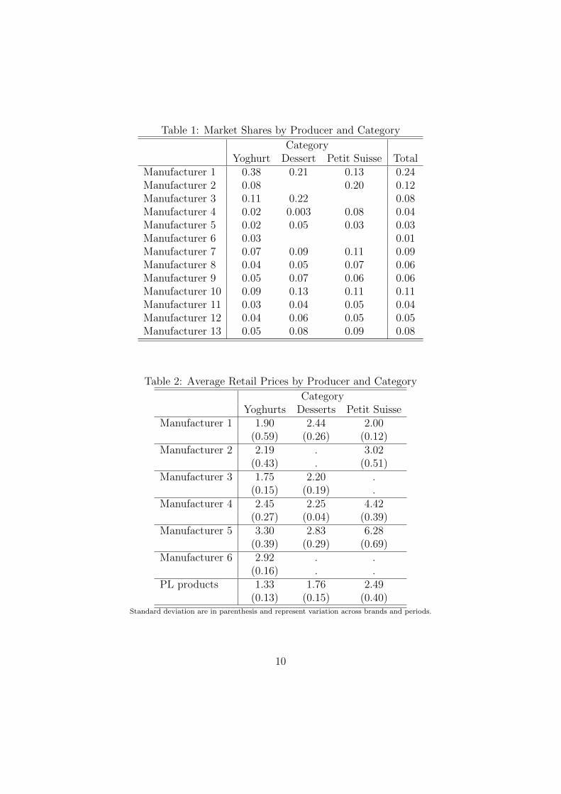
Table 1: Market Shares by Producer and Category

CategoryYoghurt Dessert Petit Suisse Total

Manufacturer 1 0.38 0.21 0.13 0.24Manufacturer 2 0.08 0.20 0.12Manufacturer 3 0.11 0.22 0.08Manufacturer 4 0.02 0.003 0.08 0.04Manufacturer 5 0.02 0.05 0.03 0.03Manufacturer 6 0.03 0.01Manufacturer 7 0.07 0.09 0.11 0.09Manufacturer 8 0.04 0.05 0.07 0.06Manufacturer 9 0.05 0.07 0.06 0.06Manufacturer 10 0.09 0.13 0.11 0.11Manufacturer 11 0.03 0.04 0.05 0.04Manufacturer 12 0.04 0.06 0.05 0.05Manufacturer 13 0.05 0.08 0.09 0.08

Table 2: Average Retail Prices by Producer and Category

CategoryYoghurts Desserts Petit Suisse

Manufacturer 1 1.90 2.44 2.00(0.59) (0.26) (0.12)

Manufacturer 2 2.19 . 3.02(0.43) . (0.51)

Manufacturer 3 1.75 2.20 .(0.15) (0.19) .

Manufacturer 4 2.45 2.25 4.42(0.27) (0.04) (0.39)

Manufacturer 5 3.30 2.83 6.28(0.39) (0.29) (0.69)

Manufacturer 6 2.92 . .(0.16) . .

PL products 1.33 1.76 2.49(0.13) (0.15) (0.40)

Standard deviation are in parenthesis and represent variation across brands and periods.

10

3 Methodology

Here we introduce the methodology used for estimating the equilibrium model,

e�ciency gains of potential mergers, and counterfactual analysis. First, we

introduce the demand and supply framework of Bonnet and Dubois (2010) that

allows us to recover the marginal cost of each product in the market. Second,

we show how Bogetoft and Wang (2005) use DEA to estimate e�ciency gains

of mergers and how we incorporate this method into the framework of Bonnet

and Dubois (2010). Using the estimated marginal costs and exogenous prices of

inputs, we are then able to recover the quantity of inputs needed to produce each

product at each time period. Finally, we present the merger simulation method

that also accounts for the new industry structure and synergy gains.

3.1 The equilibrium model

In this section, we introduce the demand and supply specification and present

the identification and estimation strategy. For the demand, we use a random

coe�cient logit model as it allows for flexible substitution patterns for consumers

between alternatives. Compared to the standard logit model, this leads to more

realistic estimates of own- and cross-price elasticities, which in turn gives better

margins and thus better estimates for marginal costs. For the supply model, we

use two-part tari↵ contracts between manufacturers and retailers, as in Bonnet

and Dubois (2010).

11

3.1.1 Demand model and identification

We use a random utility approach and in particular a random coe�cient logit

model, as in McFadden and Train (2000). We define the indirect utility function

of consumer i of buying product j at time t as:

Vijt = �b(j) + �r(j) + ↵ipjt + ⇠jt + ✏ijt, (1)

where �b(j) and �r(j) are time invariant brand and retailer fixed e↵ects,

respectively, pjt is the price of product j at time t, ✏ijt is an unobserved individual

error term that is distributed according an extreme value distribution of type

I, and ⇠jt is also unobserved by the econometrician and represents changes in

product characteristics over time. We allow for consumer heterogeneity for the

disutility of the price specifying the price coe�cient ↵i as follows:

↵i = ↵ + �vi, (2)

where ↵ is the average price sensitivity, vi follows a normal distribution that

represents the deviation to the average price sensitivity and � is the degree of

heterogeneity.

We allow for an outside option, that is, the consumer can choose another

alternative from amongst the J products of the choice set. The utility of the

outside good is normalized to zero, which means Ui0t = ✏i0t.

The mean utility is defined as �jt = �b(j) + �r(j) � ↵pjt + ⇠jt with a deviation

12

defined as ⌫ijt = ��vipjt, such that we get:

Vijt = �jt + ⌫ijt + ✏ijt. (3)

The individual probability of buying the product j takes the logit formula as

follows:

sijt ⌘exp (�jt + ⌫ijt)

1 +PJt

k=1

exp (�kt + ⌫ikt). (4)

The aggregated market share of product j is thus given by:

sjt =

Z

Ajt

sijt � (vi) dvi, (5)

where Ajt is the set of consumers buying the product j at time t and � is the

density of the normal distribution.

The own- and cross-price elasticities are given by:

@sjt

@pkt

pkt

sjt=

8>><

>>:

�pkt

sjt

Z↵isijt (1� sijt) � (vi) dvi if j = k

pkt

sjt

Z↵isijtsikt � (vi) dvi otherwise.

(6)

The unobserved term ⇠jt is likely to be correlated with price as it captures, for

example the advertising expenses of the manufacturers. Advertising influences

purchasing decisions by consumers, and as it is costly, it will certainly also a↵ect

the price. Failing to control for this unobserved product characteristic results in

a correlation between price and the error term of the demand equation, leading to

a biased estimate of the price coe�cient. In order to deal with this issue, we use

13

the two-stage residual inclusion approach (Terza et al. (2008); Petrin and Train

(2010)). In the first step, we regress prices on a set of instrumental variables

and exogenous variables of the demand equation. As instruments, we use input

prices, noted Wjt:

pjt = Wjt� + ✓b(j) + ✓r(j) + ⌘jt, (7)

where ✓b(j) and ✓r(j) are brand and retailer fixed e↵ects, respectively. The error

term ⌘jt captures the e↵ect of the omitted variables, such as advertising costs. If

we include this error term in the mean utility of the demand equation as regressor,

it captures the e↵ect of the unobserved characteristics on price. This means the

error term of the demand equation, ⇣jt = ⇠jt � �⌘jt, will not be correlated with

the price. We can then write the mean utility as:

�jt = �b(j) + �r(j) � ↵pjt + �⌘jt + ⇣jt. (8)

3.1.2 Supply model

This section presents the theoretical model we use for the supply side.

Manufacturers and retailers engage in a vertical relationship. We know that linear

pricing, where the downstream firm pays a per unit price to the manufacturer,

leads to a double marginalization problem, and profits in this chain are not

maximized. This is why the parties often use two-part tari↵s. We then use

the same empirical framework of Bonnet and Dubois (2010) to model the vertical

relationships in the dairy dessert market. We also assume that manufacturers

impose the final prices on the retailers. Bonnet et al. (2015) show that these

14

kind of contracts are preferred to linear contracts or two-part tari↵ contracts

without resale price maintenance in the dairy dessert market. Other empirical

studies suggest that this contract is used in other markets as well (Bonnet and

Requillart (2013); Bonnet and Dubois (2010); Bonnet et al. (2015)). Furthermore,

it is assumed that manufacturers have all the market power with respect to the

retailers. The game between manufacturers and retailers is then described in the

following:

Stage 1: Manufacturers simultaneously propose two-part tari↵ contracts to the

retailers. It is assumed that those contracts are public3 and consist of a per

unit wholesale price, a fixed fee, and the final price of the products.

Stage 2: After observing the o↵ers, the retailers simultaneously accept or reject

them. In case of the rejection of a retailer, they earn an exogenous outside

option. If all retailers accept, demand and contracts are satisfied.

Rey and Verge (2010) prove the existence of a continuum of equilibrium in which

consumer prices are decreasing in wholesale prices.

Let there be J di↵erent products defined by the cartesian product of brand

and retailer sets. Let there be R retailers, and Sr is the set of products sold by

retailer r. There are F manufacturers and let Gf be the set of products produced

by manufacturer f . Fj is the fixed fee paid by the retailer for selling product

j, wj is the according wholesale price and pj is the final retail price. Let sj (p)

3Following the argument of Bonnet and Dubois (2010), this assumption is justified by thenon-discrimination laws of comparable services. They argue that in the case of resale pricemaintenance only the o↵ered retail prices are essential for the decision-making of the retailers.

15

be the market share of product j, M is the total market size, and µj and cj

are the constant marginal costs of production and distribution of the product j,

respectively.

The profit of the retailer r is given by:

⇧r =X

j2Sr

[M (pj � wj � cj) sj (p)� Fj], (9)

and the profit of the manufacturer f is:

⇧f =X

k2Gf

[M (wk � µk) sk (p) + Fk], (10)

subject to the retailers’ participation constraints: 8 r = 1, ..., R, ⇧r � ⇧r.

As already explained, manufacturers make take-it or leave-it o↵ers to retailers.

However, they have to respect the participation constraint of the retailers. Let

the outside option ⇧rof the retailer be a constant that can be normalized to zero,

such that we have for the participation constraint ⇧r � 0. As Rey and Verge

(2010) show, this participation constraint is binding and can be substituted in

(10) which gives the following expression:

⇧f =X

k2Gf

[M (pk � µk � ck) sk (p)] +X

k/2Gf

[M (pk � wk � ck) sk (p)]�X

j /2Gf

Fj.(11)

Rey and Verge (2010) point out that a manufacturer internalizes the margin

of the whole vertical chain of its own products, but also internalizes the retail

margin of its competitors. We see that this profit expression does not depend on

16

the franchise fees of the manufacturer f . As the manufacturers simultaneously

propose the contracts to the retailers, the wholesale prices and the fixed franchise

fees of the other manufacturers do not a↵ect the terms of the contracts o↵ered

by the manufacturer f . Moreover, when resale price maintenance is introduced,

the wholesale prices do not a↵ect the profit of the manufacturer as it can conquer

the retail profits via the franchise fee. However, it does influence the behavior of

its competitors. The optimization problem of f then becomes:

maxpk2Gf

X

k2Gf

[M (pk � µk � ck) sk (p)] +X

k/2Gf

[M (p⇤k � w

⇤k � ck) sk (p)]. (12)

In the absence of any additional restrictions, we are not able to separately

identify the wholesale margins wk � µk and the retail margins pk � wk � ck. As

suggested by Bonnet et al. (2015), we will assume that retail margins are equal

to zero in the French dairy dessert market. The first order conditions for the

manufacturer f under this condition are given by:

sj (p) +X

k2Gf

(pk � µk � ck)@sk (p)

@pj= 0 8j 2 Gf . (13)

The first order conditions allow us to recover marginal costs mcjt as the sum of

costs of production and distribution. Note that the identified margin pk�µk� ck

is equal to wk � µk under the assumption of zero retail margins. It is useful to

denote the identified margins in matrix notation as follows:

�f + �f = � (IfSpIf )�1

Ifs (p) 8f 2 F. (14)

17

The left-hand side is the sum of wholesale (�f ) and retail (�f ) margins.4

The margins are identified as a function of estimated demand parameters that

are included in Sp, that is, the matrix of first derivatives of market shares with

respect to price. If is the diagonal ownership matrix of firm f which takes the

value 1 if the product belongs to the firm f and 0 otherwise. s (p) is the vector

of estimated market shares.

Using observed prices and estimated margins, we are able to recover marginal

costs which are then used to estimate inputs in the next step.

3.2 Merger simulation

When assessing the implications of a merger, two main factors are in opposition.

First, the change in industry implies an upward pressure on price, as the market

power of the merged firm increases. Competitors also benefit from the decreased

competitive pressure by increasing their prices. The second factor is the change

of the cost structure of the merged firms. Synergies may reduce marginal

production costs that firms can partially or completely transmit to final retail

prices. Competitors have to follow and cut prices to prevent their customers

from switching. The question is, what is the net e↵ect on the price of these two

opposing forces?

In this section, we present the methodology used to estimate cost savings

from a potential merger, on the one hand, and the methodology used to evaluate

the price e↵ect of a merger — taking into account the estimated cost saving

and the change of the industry — on the other hand. Section 3.2.1 describes

4Note that in our selected equilibrium, the latter one is equal to zero.

18

the source of potential cost savings. In Sections 3.2.2 and 3.2.3, we present the

methodology on how we estimate the potential savings of production inputs. The

method presented in Section 3.2.3 requires data on the inputs and the outputs

of manufacturers. In Section 3.2.2, we show how we obtain these quantities from

our data. Section 3.2.4 shows how we translate the input savings into marginal

cost reductions, and finally, Section 3.2.5 describes how we simulate the new price

equilibrium post merger and how we assess the e↵ect on consumer surplus.

3.2.1 Synergies

Cost e�ciencies are a major argument used by firms to justify a proposed merger

in front of the regulatory authorities. Gugler et al. (2003) showed that synergies

are present in about one third of the mergers. In this section, we discuss where

synergies stem from in general, the relevant merger gains to focus on and we

examine their suitability in the French dairy dessert industry.

Farrell and Shapiro (1990) describe three sources of merger gains. First, the

merged firms can distribute their output across the participating firms, moving

production to the more e�cient production sites. This would not change the

firms’ knowledge or capital intensity. The changes in marginal costs and the

associated gains are due to a reallocation to the production site with lower

marginal costs pre-merger. Second, firms can shift capital from one firm to

another in order to operate at a higher scale. Farrell and Shapiro (2001) argue

that merger benefits that are due to economies of scale cannot be used to justify

a merger in most cases. This is because if firms can reach a higher scale of

production, and thus benefit from lower production costs without a merger, the

19

benefits of a merger can be realized without an increase in market concentration

which would be potentially harmful for consumers. They further explain that

in the general case, market pressure should force firms to produce at a higher

scale if possible, making a merger unnecessary. Third, firms can learn from each

other. This involves the sharing of knowledge and management skills, or taking

advantage of complementary patents. This could lead to a change in marginal

cost after a merger. In this case, the marginal cost reduction is derived from

economies of scope or harmony e↵ects (Bogetoft and Wang (2005)).

An important question in this paper is identifying the source of synergies

which is most likely to occur in the French dairy dessert industry. The main input

ingredient of any yoghurt or other dairy desserts is raw milk. In the production

process, there are multiple highly-automated steps that the raw milk goes through

in order to transform it into an input that can be used in the final product. The

first steps (clarification and standardization) in the production process usually

involve multiple rounds in centrifuges and cooling and heating phases in order to

ensure a homogeneous input that meets certain requirements, such as fat content.

Depending on the final product, di↵erent steps then follow which are automated

and firm specific. Each company is likely to be e�cient in some of the steps

in the production process that are crucial for their specific products. Certain

products require certain procedures in order to obtain the desired consistency

and water content, which makes each firm an expert in the method it uses in the

production process. After a merger, this firm-specific expertise is shared among

the merging firms, such that we expect that in this industry, technological transfer

and management skills are the main source of merger gains (Brush et al. (2011)).

20

Another important factor is the number of people involved in the production

process. A firms’ technical sophistication should also be reflected in the number

of workers required for production. A more technically-advanced firm requires

fewer workers to produce a certain amount of output; that is, better management

can make use of a workforce more e�ciently. After a merger, technical transfer

and introduced management skills should also carry over to the less e�cient firm

in terms of manpower e�ciency.

3.2.2 Inputs and outputs

After obtaining marginal costs mcjt from the equilibrium model, in order to

calculate synergy gains, we need definitions for inputs k 2 K and outputs. As

we have to make outputs of arbitrary firms comparable, it is convenient to define

a product by its category c 2 C. We then distinguish the outputs between the

three di↵erent categories: yoghurts, fromage frais and petit suisse, plus other

dairy desserts. This means that each firm f 2 F can produce three di↵erent

kinds of products. The total output of firm f of product category c is given

by its total quantity of products yfc = Msfc in this category, where sfc is the

market share of firm f in the product category c and M is the total market size.

We assume that production technologies in each category across firms di↵er in

e�ciency. We estimate inputs by regressing marginal costs on input prices gkt

and we assume that the marginal cost of product j in period t has the following

specification:

21

mcjt =X

f2F

�f(j)c(j) +X

r2R

�r(j) +X

f2F

X

c2C

X

k2K

�f(j)c(j)kgkt + ✏jt. (15)

As marginal costs are the costs of producing one unit,5 the estimated

coe�cients �f(j)c(j)k can be interpreted as the amount of input k needed to

produce one unit. �f(j)c(j) are fixed e↵ects for each firm and category that

capture unobserved cost shifters that vary across firms and product categories.

�r(j) are retailer fixed e↵ects and capture retailer specific costs, such as costs of

warehousing and distribution. The total amount of input k for product category

c of firm f is given by xfck = Msfc�fck. A firm f is characterized by its input

and output vector xf and y

f , respectively.

3.2.3 Estimating potential merger gains with DEA

We now introduce the method that allows us to estimate the potential gains ex

ante using Data Envelopment Analysis (DEA).6 Following Bogetoft and Wang

5We assume a constant return to scale production technology. Under this assumption, wecan use the marginal costs as average costs. (cf Footnote 11 in Subsection 3.2.3 for a justificationof this assumption)

6DEA is a non-parametric method for production frontier estimation and is used to measurethe e�ciency of a single firm within an industry. The basic idea of the e�ciency measure islinked to Farrell (1957) who argues that the e�ciency of a firm is assessed by its distance tothe production possibility set of the industry. The method wraps a tight fitting hull around theinput/output data of the entire industry, such that it satisfies certain assumptions that vary,depending on the specification of the technology. The e�ciency of a firm is then measuredby its distance to this hull, also called frontier. For a more fundamental introduction, see forexample, “Introduction to Data Envelopment Analysis and Its Uses” by Cooper et al. (2005).

22

(2005), the production possibility set T (x, y) is defined as:

T =�(x, y) 2 RK+C

+

|x can produce y . (16)

In the following, we introduce how synergy gains are estimated in this

framework. First, we introduce the “potential overall gains” of merging, which

is a maximal benchmark of potential savings. Then, in order to receive more

realistic potential savings, “adjusted overall gains” are introduced, which control

for the individual ine�ciency of the merging firms. In the third step, the concept

of “input slacks” is introduced, allowing us to calculate additional savings that

are not captured in the previous step. At the end of this section, we provide three

examples to illustrate the importance of the assessment of adjusted overall gains

and input slacks.

Potential overall gains

In order to measure the potential synergy gains of a merger, the inputs and

outputs of the merged entity are pooled together, pretending that it is in fact

one firm, and then the distance of this artificial firm to the frontier is measured.

There are several ways to conduct this projection. We use the input-oriented

view, as this can be converted to cost savings. With this approach, the e�ciency

of firm f is measured by how much we can reduce the inputs of this firm and

produce the same amount of outputs in comparison to the industry frontier. Let

us define the set of firms that merge as U . Pooling the inputs and outputs of all

23

f 2 U and projecting it on the frontier gives the “potential overall gains” from

merging, and is described by the following program:

E

U = Min

(E 2 R

�����

E ⇤

X

f2U

x

f,

X

f2U

y

f

!2 T

). (17)

This translates into the following optimization problem:

minE,�

E s.t.

E ⇤"X

f2U

x

f

#�

X

f2F

�

fx

f

X

f2U

y

f X

f2F

�

fy

f

� � 0

(18)

As E is a scalar, it reflects the proportional reduction of inputs that is possible

compared to the e�cient industry frontier. The condition � � 0 comes from the

constant return to scale assumption.7 The measure E

U simply represents the

ine�ciency of the combined inputs and outputs of the merging firms U . It allows

7DEA can be performed under di↵erent assumptions in terms of the underlying productiontechnology T of the considered sector. The returns to scale property plays a crucial role as theshape of the estimated frontier depends on this property. Potential merger gains are calculatedusing the distance of the combined firm’s inputs and outputs to the frontier. This means themerger gains are dependent on the shape of the frontier. Thus, it is crucial to provide a goodjustification for the chosen technology. As explained in Section 3.2.1, the source of mergergains we focus on is learning and technology sharing. Following the argument of Farrell andShapiro (2001), we rule out increasing returns to scale. Furthermore, following Bogetoft andWang (2005), we assume that after a merger, firms could further operate as two single firmsand simply coordinate prices without further integration. This rules out decreasing returns toscale. In order to capture synergies derived from economies of scope, we will then use a constantreturns to scale (CRS) production technology.

24

us to compute the amount of reduction (1-EU) in percentage of the inputs used

by the merged firms to reach the industry frontier. Note that EU captures more

than the synergy e↵ects that are due to economies of scope as it also contains

the individual ine�ciency of the individual merging firms (Bogetoft and Wang

(2005)).

Adjusted Overall Gains

As we aim to extract the e↵ects that are due to learning from amongst the

merging firms, we have to remove the e↵ect due to the technical ine�ciency of

the individual firms. Following Bogetoft and Wang (2005), we decompose the

“potential overall gains from merging” E

U into the “adjusted overall gains” E

U⇤

and individual ine�ciency T

U in such a way that we have:

E

U = E

U⇤ ⇤ TU. (19)

Bogetoft and Wang (2005) propose to first project the inputs of the individual

firms on the frontier and then use these adjusted inputs in the merger analysis.

This way individual ine�ciency is taken care of, and the resulting e�ciency

measure of the pooled adjusted inputs only reflect the synergy e↵ects due to

learning or economies of scope. EU⇤is given by:

E

U⇤= Min

(E 2 R

�����

E ⇤

X

f2U

E

fx

f,

X

f2U

y

f

!2 T

). (20)

25

We see that the only di↵erence between E

U⇤and E

U is that we multiply the

input vector of the individual firm f , that is part of the merger U , by its e�ciency

score E

f obtained from a first step where we projected the single firms on the

frontier.8

Input slacks

Thus far, we have been considering a linear reduction in inputs, which is

a proportional decrease of all inputs by�1� E

U⇤� ⇤ 100%. However, it is likely

that after this proportional reduction, there is still the possibility of input specific

reductions. Ji and Lee (2010) refer to this as “input slacks”. Bogetoft and Wang

(2005) mention this possibility but do not implement it. Here, we make use of

this option and add the input slacks to allow for nonlinear reductions in inputs.

Intuitively, the achieved savings in this case are at least as high as in the linear

case, because the input slacks are on top of the linear part.

We define the input slack for input k of the merged entity U as SUk . Let xU

k

be the pooled total amount of input k for the entity U . Then the reduced input

k post merger is given by:

E

U⇤x

Uk � S

Uk . (21)

We want to express the savings of input k of U in a single score E

Uk similar to

8This first step is a standard DEA with a CRS technology using all initial firms. From this,the e�ciency scores Ef are obtained and are then used to adjust the inputs of the mergingfirms.

26

the e�ciency scores obtained from the DEA but input specific. Following Cooper

et al. (2005), this is given by:

E

Uk ⇤ xU

k = E

U⇤ ⇤ xUk � S

Uk . (22)

The first term of the right-hand side E

U⇤x

Uk is the linear part of the reduction.

In addition to this, we subtract the input specific reduction S

Uk . We want to

express the total reduction of each input as an input specific score E

Uk . We have

all information such that we can solve for EUk , as follows:

E

Uk =

E

U⇤ ⇤ xUk � S

Uk

x

Uk

. (23)

Examples

To illustrate the three di↵erent parts that have been formally introduced,

consider the following examples. There are two firms, A and B, neither of which

are located on the frontier, and that produce both one product y with two inputs

x

1

and x

2

. Let us assume that at the e�cient industry frontier, in order to produce

y = 10 outputs, x1

= 4 and x

2

= 4 inputs are required. Let us distinguish three

di↵erent settings of this market to illustrate the three parts shown before: a) firms

use the same technology; b) firms use di↵erent technology symmetrically; and c)

firms use di↵erent technology asymmetrically.9 In a), both firms are equally

e�cient. This means that they need the same number of inputs to produce the

same number of outputs, that is, y = 5, xA1

= 5 and x

A2

= 5 and x

B1

= 5 and

9Table 7 in the Appendix summarizes the results of the three examples.

27

x

B2

= 5. In this setting, both firms use the same production technology, and

we would not expect any merger gains that are due to economies of scope or

learning, as the firms are equal. However, in this setting, the measure E

U would

predict merger gains as follows. When inputs and outputs are pooled, we have

y = 10, xU1

= 10 and x

U2

= 10. We can reduce both inputs by 60% compared to

the frontier because we then hit the frontier in both input dimensions. This now

means that we have E

U = 0.4 because 0.4 ⇤ x

U1

= 4. This example shows that

two equal firms would produce synergy gains using E

U . These synergies are due

to both firms’ individual ine�ciency pre-merger, as the example illustrates.

Consider now the example in setting b) where neither firm is located on the

frontier but use di↵erent production technologies. Let us now assume that firm

A uses xA1

= 4 and x

A2

= 6 and firm B uses xB1

= 6 and x

B2

= 4 to produce y = 5

outputs each. Let the e�cient frontier be y = 5 and x

1

= 2 and x

2

= 2. We

see that both firms are ine�cient compared to the frontier, but firm A has an

advantage in input 1 compared to firm B and firm B has an advantage in input 2

compared to firm A. The program E

U (without removing individual ine�ciency)

would produce the following savings. Combining both firms’ inputs and outputs

we have y = 10, xU1

= 10 and x

U2

= 10. We can reduce both inputs by 60%

because we then hit the frontier in both dimensions. This implies that EU = 0.4.

This again contains individual ine�ciency plus the gains that are due to learning.

If we now project the individual inputs (without pooling) on the frontier we get

E

A = 0.5, EA ⇤ xA1

= 2 and E

A ⇤ xA2

= 3 for firm A and E

B = 0.5, EB ⇤ xB1

= 3

28

and E

B ⇤xB2

= 2 for firm B.10 Next, if we pool these adjusted inputs and outputs

we have y = 10, xU1

= 5 and x

U2

= 5. After adjusting and pooling the individual

inputs, we again look at the amount by which we can proportionally reduce these

inputs compared to the industry frontier. In this example, this delivers EU⇤= 0.8

as E

U⇤ ⇤ x

U1

= 4 and E

U⇤ ⇤ x

U2

= 4. This implies the following decomposition:

E

U = 0.4, EU⇤= 0.8 and T

U = 0.5. Here we see that the relatively large savings

that are due to E

U can be deceiving, and once individual ine�ciency is controlled

for the potential savings that are due to economies of scope are much smaller.

The individual ine�ciency scores Ef = 0.5 are reflected in the decomposition with

T

U = 0.5.11 The di↵erence between a) and b) is that in a) the adjusted overall

gains are zero, whereas in b) they are 20%, and this shows how the mechanics of

generating synergies of this method works. Specifically, this demonstrates how

firms can benefit from each other when they have comparative advantages in

di↵erent inputs.

The asymmetric case c) is similar to case b) except that now firm B requires

x

B1

= 8. Conducting the same exercise as in b) delivers E

U⇤= 0.8. However,

note that after multiplying the pooled and adjusted input xU1

= 6 with E

U⇤= 0.8

we obtain 4.8 which does not reach the frontier which is located at x

1

= 4. So

there is further room for additional reductions of 0.8 in this input dimension.

This further reduction is captured by the input slacks, which appear when the

10Ef represents the individual ine�ciency score. Here we have EA = EB because of asymmetric example. However, in general, this is not the case.

11In this example, individual ine�ciency scores Ef coincide with TU . This is due to theconstructed symmetric example and does not hold in general.

29

merging firms do reach the frontier in all input dimensions, after adjusting for

individual ine�ciency and proportionally reducing the inputs by E

U⇤

3.2.4 Marginal cost reduction

As EUk represents the input specific synergy gains from merger U , we can reduce

the output k of the merged entity by (1�E

Uk ) ⇤ 100%. The new marginal cost of

the merged entity U is given by:

mcjt =

8>><

>>:

mcjt ��P

k2K�1� E

Uk

��f(j)c(j)kgkt

�for j 2 U,

mcjt otherwise,

(24)

where �f(j)c(j)k is the estimated input k from the cost estimation that is used by

firm f to produce output c. This estimated input is multiplied by the possible

reduction�1� E

Uk

�, and the input price gkt, as we want to subtract only the

savings in Euros from the initial marginal costs mcjt.

3.2.5 Price e↵ects

In this section, we present the general methodology used to assess the e↵ects of

the change in the industry structure and cost savings on prices. The simulation

is performed using the following program:

min{p⇤jt}j=1,...,J

��p

⇤t � �

�p

⇤t , I

⇤1

, ..., I

⇤F�1

�� �

�p

⇤t , I

⇤1

, ..., I

⇤F�1

�� mct

��, (25)

where ��p

⇤t , I

⇤1

, ..., I

⇤F�1

�and �

�p

⇤t , I

⇤1

, ..., I

⇤F�1

�are, respectively, the margins of

manufacturers and retailers as a function of new equilibrium prices and new the

30

ownership structure. The first three terms represent the marginal costs derived

from the new price equilibrium, which should be equal to the new marginal costs

mct in (24).

As we aim to isolate the price variation for the two opposite forces, we also

simulate the price e↵ects for two benchmark cases. On the one hand, we use the

change in the industry structure only, then mcjt = mcjt, and on the other hand,

we use marginal cost savings only, then�I

⇤1

, ..., I

⇤F�1

�= (I

1

, ..., IF ).

We also compare our results to the common practice of reducing all marginal

costs by 5% post merger. In this case, the new marginal costs post merger mcjt

are equal to 0.95 ⇤mcjt for merging firms and mcjt for non-merging firms.

Furthermore, it is interesting to compare the impact on consumer surplus and

the profit of the industry with and without synergies. Following Bonnet and

Dubois (2010), consumer surplus is given by:

CSt (pt) =1

|↵i|ln

JX

j=1

exp [Vijt (pt)]

!. (26)

4 Empirical results

First, we discuss the results of the demand estimation, implied price-cost margins

and the marginal costs. Then we present the results of the Data Envelopment

Analysis and the e↵ects of the four proposed mergers.

31

4.1 Demand estimates, price elasticities and margins

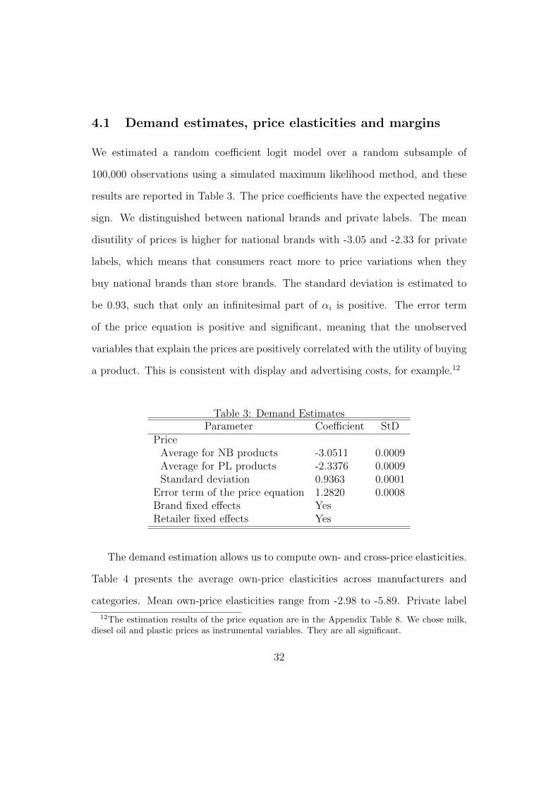
We estimated a random coe�cient logit model over a random subsample of

100,000 observations using a simulated maximum likelihood method, and these

results are reported in Table 3. The price coe�cients have the expected negative

sign. We distinguished between national brands and private labels. The mean

disutility of prices is higher for national brands with -3.05 and -2.33 for private

labels, which means that consumers react more to price variations when they

buy national brands than store brands. The standard deviation is estimated to

be 0.93, such that only an infinitesimal part of ↵i is positive. The error term

of the price equation is positive and significant, meaning that the unobserved

variables that explain the prices are positively correlated with the utility of buying

a product. This is consistent with display and advertising costs, for example.12

Table 3: Demand EstimatesParameter Coe�cient StD

PriceAverage for NB products -3.0511 0.0009Average for PL products -2.3376 0.0009Standard deviation 0.9363 0.0001

Error term of the price equation 1.2820 0.0008Brand fixed e↵ects YesRetailer fixed e↵ects Yes

The demand estimation allows us to compute own- and cross-price elasticities.

Table 4 presents the average own-price elasticities across manufacturers and

categories. Mean own-price elasticities range from -2.98 to -5.89. Private label

12The estimation results of the price equation are in the Appendix Table 8. We chose milk,diesel oil and plastic prices as instrumental variables. They are all significant.

32

products have the most elastic demand in all product categories. In the yoghurt

category, manufacturers 1 and 3 have the least elastic demand. The second

column suggests that no national brand producer has more market power than the

others in the other dairy desserts category. In the third category, manufacturer

5 enjoys the most market power. Similar own-price elasticities were found by

Draganska and Jain (2006) and Bonanno (2012) that ranged between -2.45, -6.25

and -1.4, -6.86, respectively.

Table 4: Own Price Elasticities

Yoghurts Other DairyDesserts

Fromage Blancand Petit Suisse

Manufacturer 1 -3.67 (0.48) -4.12 (0.09) -3.94 (0.10)Manufacturer 2 -4.05 (0.17) -4.10 (0.13)Manufacturer 3 -3.67 (0.26) -4.06 (0.12)Manufacturer 4 -4.14 (0.07) -4.11 (0.03) -3.59 (0.18)Manufacturer 5 -4.05 (0.14) -4.17 (0.05) -2.98 (0.18)Manufacturer 6 -4.18 (0.04)PL products -4.19 (0.29) -4.98 (0.24) -5.89 (0.34)

Standard deviations are in parenthesis and represent variation across brands, retailers andperiods.

The average implied price cost margins are reported in the Appendix in Table

9 across categories and manufacturers. On average, the total margin is 37%

for yoghurt products, 32% for other dairy desserts and 29% for fromage frais

and petit suisse products. Manufacturer 1 has the strongest market power given

that the average margin of its products are the highest for the three categories,

49%, 40% and 44%, respectively. Manufacturer 3 exhibits the second largest

margins with respect to the other firms. The lowest margins are for the private

33

label products in each category. In total, the margins range between 17% and

49%. Other authors find similar margins: Bonanno (2012) recovers margins that

range between 16% and 68%; and Villas-Boas (2007) finds margins that range

between 12.8% and 45.8% in the preferred supply model. Regarding the results on

marginal costs in the Appendix in Table 10, they seem to be consistent. In total,

manufacturer 1 has the lowest marginal costs closely followed by manufacturer

3 and PL products. These three manufacturers have very similar low marginal

costs for yoghurts and other dairy desserts. In the yogurt category, the marginal

cost is higher for manufacturers 5 and 6 as they also use other milks that are more

expensive than cow milk, such as soy milk or sheep and goat milks. As expected,

the marginal costs of producing fromage frais and petit suisse and other dairy

desserts are higher.

4.2 Cost function and DEA

For the estimation of the cost function, we use input prices from the French

National Statistic O�ce (INSEE). We remain consistent with economic theory,

as in Gasmi et al. (1992), we impose the positivity of the parameters �fck, and

therefore, we use a non-linear least square method. We have chosen to use milk

and salary as inputs, as they are the main inputs required to produce dairy

products.

We present the results of the DEA in Table 5. In total, the DEA is performed

with 13 initial firms that are shown in the upper part of Table 5 and 78 constructed

mergers of which we show three selected mergers at the bottom part of Table 5.

34

In total, we have 91 decision-making units with two inputs and maximal three

outputs.

For the initial firms, we show the first stage e�ciency scores Ef that are used

to adjust the inputs before they are pooled to construct the mergers. A value of

1 means that this firm is part of the industry frontier, which is the case for five

out of 13 firms.

At the bottom part in columns 2-4, the merger specific e�ciency measures

are given.13 The first EU⇤in column 2 shows the linear e�ciency scores from the

DEA. For the mergers, this score is already adjusted for individual ine�ciency.

Thus, all inputs of a given firm that is part of the merger can be reduced by

multiplying the inputs with the respective e�ciency score and keeping the output

constant. The implied input specific e�ciency scores are given in columns 3 and

4 for milk and salary, respectively. These are also the scores that are used to

calculate the savings in marginal costs in column 5. In the three mergers we

consider, the input specific e�ciency scores are equal to the linear e�ciency score

in column 2. This means that there is no further input specific reduction in inputs

possible.

The last column shows the average adjusted potential savings in marginal

costs in percent, and the standard deviation across products, and time periods

within the merged entity are shown in parenthesis. Even though the input savings

are the same for a given product category and firm, the percentages vary as the

original marginal costs are di↵erent. The savings of the selected mergers range

13We use the bootstrap estimator presented in Kneip et al. (2008). In each bootstrap sample,we use 50% of the original sample size as the naıve approach leads to inconsistent results, aspointed out by Kneip et al. (2008)

35

between 1.88% and 7.84%.14

Table 5: DEA - Constant Returns to Scale

Manufacturers Ef Manufacturers Ef

Manufacturer 1 0.57 Manufacturer 8 0.92Manufacturer 2 0.97 Manufacturer 9 0.75Manufacturer 3 0.85 Manufacturer 10 1Manufacturer 4 0.91 Manufacturer 11 0.78Manufacturer 5 1 Manufacturer 12 0.77Manufacturer 6 1 Manufacturer 13 1Manufacturer 7 1

Mergers E

U⇤E

UmE

Us Average MC SavingsM1 - M3 0.86 0.86 0.86 7.84% (3.78)M1 - M11 0.97 0.97 0.97 1.88% (0.97)M8 - M9 0.92 0.92 0.92 3.37 % (2.03)

Standard deviation across products and periods in parenthesis.

4.3 Merger simulation and welfare

We consider three potential mergers. The initial HHI in the French dairy dessert

industry is 1,160.15 The M1-M3 merger combines the pre-merger market shares

of 24% and 8%, respectively. The change of the HHI is more than 250 and

14Table 14 in the Appendix summarizes mean savings of all 78 possible bilateral mergers.First note that only about 56% of the possible mergers are predicted to produce any e�ciencysavings at all. If we neglect the mergers that produce relatively small e�ciencies and onlyconsider mergers with at least 3% savings, then only about 35% of the mergers produce synergygains. This means that about 44% of the mergers do not produce e�ciency gains and are likelyto harm consumers. Other authors find similar results. Our results are consistent with Gugleret al. (2003) who make use of a large panel data set to analyze merger e↵ects of companiesworld-wide that occured during the 15 years prior to 2003. They find that approximately 29%of the mergers produced e�ciency gains.

15Note for the calculation of the HHI and the changes post-merger, we assume that eachprivate label manufacturer is treated as a single firm.

36

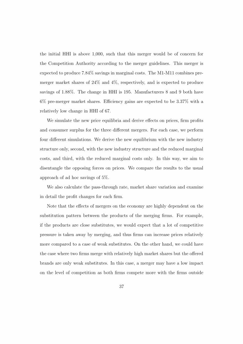
the initial HHI is above 1,000, such that this merger would be of concern for

the Competition Authority according to the merger guidelines. This merger is

expected to produce 7.84% savings in marginal costs. The M1-M11 combines pre-

merger market shares of 24% and 4%, respectively, and is expected to produce

savings of 1.88%. The change in HHI is 195. Manufacturers 8 and 9 both have

6% pre-merger market shares. E�ciency gains are expected to be 3.37% with a

relatively low change in HHI of 67.

We simulate the new price equilibria and derive e↵ects on prices, firm profits

and consumer surplus for the three di↵erent mergers. For each case, we perform

four di↵erent simulations. We derive the new equilibrium with the new industry

structure only, second, with the new industry structure and the reduced marginal

costs, and third, with the reduced marginal costs only. In this way, we aim to

disentangle the opposing forces on prices. We compare the results to the usual

approach of ad hoc savings of 5%.

We also calculate the pass-through rate, market share variation and examine

in detail the profit changes for each firm.

Note that the e↵ects of mergers on the economy are highly dependent on the

substitution pattern between the products of the merging firms. For example,

if the products are close substitutes, we would expect that a lot of competitive

pressure is taken away by merging, and thus firms can increase prices relatively

more compared to a case of weak substitutes. On the other hand, we could have

the case where two firms merge with relatively high market shares but the o↵ered

brands are only weak substitutes. In this case, a merger may have a low impact

on the level of competition as both firms compete more with the firms outside

37

the merger. This is also recognized by the Competition Authority in the merger

guidelines.

Table 6 summarizes the results of the four simulations for the three merger

cases. Columns 2-4 represent the three di↵erent mergers. For each of the mergers,

we analyze the e↵ects on prices and profits of the industry, and the prices and

profits of the merged and outside firms separately.16 As we are interested in the

e↵ects of mergers on consumers, we also present the changes in consumer surplus.

Benchmark

When we take into account the change of the industry structure only and the

reduced marginal costs only, these results can be viewed as benchmark results.

The former is a worst case and the latter a best case scenario from the consumers’

perspective. We see that without cost savings, all figures behave as expected in

all three mergers. Industry prices17 and industry profits increase and consumer

surplus decreases as expected. The merged firms benefit more than the average

outside firm. Also price reactions are larger for the merged firm than the average

industry price changes.

The other benchmark case — when we do not take into account the change

in industry structure and look at the e↵ects of the reduced marginal costs only

— also show consistent results. As in this setup, there is only the downward

16Note that we cannot identify the fixed fees; in which case we are then only able to computeindustry profit, that is, the sum of retail and manufacturer profit

17Industry price changes are computed as the weighted average (by market share) of pricechanges over all products in the industry.

38

pressure on prices, we see that all prices of the merged entity and the outside

firms decrease in all cases. Note that we would expect that only the firms that

experience the reduced cost would benefit in this new market equilibrium and the

e↵ect on total industry profit is therefore ambiguous. Indeed, we see that indeed

only firms that have lower marginal costs increase their profits. The higher the

marginal cost savings, the more they benefit. The firms with cost reductions now

have a larger margin and thus have an incentive to decrease prices in order sell to

more consumers. All the outside firms lose in the new equilibrium. As a reaction

to the price cuts by the firms with lower marginal costs, outside firms cut prices

as well and lose, as they do not enjoy any cost reductions to compensate for

the lower prices. Industry profits increase in all three cases. Consumer surplus

always increases, which is consistent with economic intuition, as reduced costs

should always benefit the consumers without changes in the industry structure.

Net e↵ect

In this section, we discuss the results of the scenario when we take into account

both the change in industry structure and the reduction of marginal costs.

The M1-M3 merger produces the highest e�ciency gains of the three mergers

we consider, and also represents the largest increase in market concentration.

Table 11 shows that the merging parties are also the main competitors of each

other according to the substitution patterns. We see that industry prices actually

decrease by 0.33%. Merged firms decrease prices to a larger extent by 1.81%.

Here, the upward pressure on prices can be outweighed by the marginal cost

reductions. Industry profits increase by almost 6%. This large increase is driven

39

by the increase in the merging parties profits. Table 17 shows profit changes for

each firm. Manufacturers 1 and 3 gain 17.39% and 19.10%, respectively. Outside

firms lose between 1.20% and 1.83%. Interestingly, the post-merger strategy for

both merging firms appears to be di↵erent. Table 15 shows that manufacturer

1 decreases and manufacturer 3 increases its prices post merger.18 The merging

parties seem to shift consumers from manufacturer 3 to manufacturer 1 by this

pricing policy post merger. Table 9 shows that manufacturer 1 has the higher

margin and also the higher market share pre-merger giving the merged entity

incentives for this kind of strategy. Consumer surplus in this scenario increases

by 0.92%, which is a large di↵erence to the merger scenarios without e�ciency

gains and the ad hoc 5% rule, which predicts a decrease in consumer surplus of

1.1% and a very slight increase of 0.17%, respectively.

The M1-M11 merger results in a medium change of industry concentration of

more than 195 of the HHI and low savings of less than 2%. The reductions in

marginal costs are just enough to compensate for the increase in concentration,

which means that industry prices show minimal change, and rise only slightly

by 0.06%. Merging firms increase prices by 0.37%. Industry profits increase by

1.63%. Merging firms benefit more than outside firms. Table 17 shows that

manufacturers 1 and 11 gain 4.63% and 2%, respectively. Outside firms gain

around 0.3% each. The strategy employed is similar as in the merger between

manufacturers 1 and 3. As shown in Table 15, the extremely negative pass-

through rate of manufacturer 11 indicates a relatively large price increase post

merger. At the same time, manufacturer 1 decreases its prices slightly. Again,

18A negative pass-through rate means that prices have increased after a cost reduction.

40

this suggests that the merging parties make consumers switch from manufacturer

11 to 1. Manufacturer 1 has a much higher margin and a higher market share.

Consumer surplus decreases by 0.16%, making the merger anti-competitive. The

5% ad hoc rule delivers completely di↵erent results. It overstates the pro-

competitive e↵ects and predicts an increase of 0.66% in consumer surplus.

The merger between manufacturers 8 and 9 increases concentration by only

67 in HHI. The merger produces medium cost savings of 3.37%. We expect

this merger to increase consumer surplus, as the downward pricing pressure is

likely to outweigh the upward pricing pressure, as the increase in concentration

is relatively small. Industry prices decrease by 0.14%. Merging firms decrease

prices by 1.87%. Industry profits increase by 0.60%. The merging parties largely

benefit from this merger as they increase profits by 12.83%. Outside firms lose

0.70% on average. Table 15 shows that both firms decrease prices post merger.

As expected, consumer surplus increases post merger by 0.38%. The 5% ad hoc

rule overstates the pro-competitive e↵ects.

A notable detail of the presented results is that marginal cost savings and

concentration e↵ects seem to have an equal weight for the market outcome post

merger for all e↵ects, except for the profits of the merged entities. This can be

seen in Table 6, where for most e↵ects the net e↵ect is approximately an average of

the two benchmark cases. However, the changes in profits of the merged entities

are almost only driven by cost savings. The benchmark results show that profit

changes, when we only take into account synergy gains, are almost the same as

profit changes, when we take into account both forces. Even in the case of M1-M3

41

with a relatively large increase in concentration, the changes in profits are almost

only driven by synergy gains. This is an important result, as the main incentive

to merge is the expected profit change. Our results suggest that managers are

more likely to neglect the positive e↵ect of concentration, and instead focus on

possible synergy gains as the main driver for profit changes. Furthermore, post-

merger pricing can be complex and may involve asymmetric pricing in order to

encourage consumers to switch from one firm to the other.

42

Table 6: Merger E↵ects

ManufacturersE↵ects\Merger M1 - M3 M1 - M11 M8 - M9

Cost Savings 7.84% (3.78) 1.88% (0.97) 3.37% (2.03)HHI (�HHI) 1550 (390) 1355 (195) 1227 (67)PricesIndustryOnly Merger 0.56% (0.22) 0.25% (0.01) 0.07% (<0.01)Merger+Sav -0.33% (0.03) 0.06% (0.01) -0.14% (0.01)Only Sav -0.97% (0.02) -0.20% (0.01) -0.22% (0.01)5 Percent -0.04% (0.02) -0.28% (0.01) -0.22 (<0.01)

Merged firmsOnly Merger 3.08% (0.07) 1.58% (0.05) 0.95% (0.2)Merger+Sav -1.81% (0.18) 0.37% (0.04) -1.87% (0.05)Only Sav -5.34% (0.15) -1.26% (0.04) -2.93% (0.07)5 Percent -0.22% (0.09) -1.77% (0.06) -2.90% (0.04)

ProfitsIndustryOnly Merger 1.51% 0.87% 0.33%Merger+Sav 5.80% 1.63% 0.59%Only Sav 3.82% 0.69% 0.17%5 Percent 4.15% 3.06% 0.67%

Merged firmsOnly Merger 0.59% 0.39% 0.11%Merger+Sav 17.80% 4.36% 12.83%Sav 16.88% 3.93% 12.68%5 Percent 11.27% 11.93% 19.59%

Outside firmsOnly Merger 2.08% 1.10% 0.36%Merger+Sav -1.73% 0.30% -0.70%Sav -4.38% -0.88% -1.15%5 Percent -0.33% -1.25% -1.33%

Cons. SurplusOnly Merger -1.1% -0.58% -0.19%Merger+Sav 0.92% -0.16% 0.38%Only Sav 2.40% 0.47% 0.62%5 Percent 0.17% 0.66% 0.71%

43

5 Conclusion

Evaluating mergers is one of the key tasks of competition authorities. Empirical

tools have become more sophisticated, taking into account strategic e↵ects as well

as vertical structure and contracts used within the vertical structure. However,

one of the main aspects in mergers are the potential synergy gains that can arise

post merger. So far, merger simulation models rely on ad hoc assumptions about

cost reductions, or the models are used to find the required cost reductions to

make a merger worthwhile. Other research aims at quantifying synergy e↵ects

due to fixed costs savings by reducing the product space.

In this article, we present an integrated approach to estimate e�ciency gains

and incorporate them into the merger simulation. We estimate a structural

demand and supply model taking into account the vertical structure of the

market. The contribution of this article is to use Data Envelopment Analysis in a

next step, in order to derive synergy gains of potential mergers, and incorporate

them into the structural model. We implement this methodology in the French

dairy dessert market, and we simulate the impact of some bilateral mergers, taking

into account the new ownership configuration and marginal cost savings. We find

that only about 56% of the mergers produce any synergy gains, meaning that

roughly half of the mergers do not produce any synergy gains and are therefore

considered to be anti-competitive. The average marginal cost reductions are

2.55%, which implies that the ad hoc rule of 5% savings overstates the pro-

competitive e↵ects of mergers in the French dairy dessert industry. Depending

on the marginal cost savings, the e↵ects on prices, profits and consumer surplus

44

di↵er. We find that the upward pressure on prices after a merger can be

outweighed by the downward pressure, due to reduced marginal costs if savings

are large enough. By isolating the concentration and e�ciency e↵ects on profits,

prices and consumer welfare, we show that potential savings are just as important

as market concentration. However, incentives to merge are fully driven by cost

savings. Concentration e↵ects on profits of the merging firms are relatively small

compared to the e↵ects that are due to cost savings. This suggests that policy

makers require more reliant tools in order to screen mergers for their potential

e�ciency gains. Furthermore, our results suggests that firms may want to shift

consumers from one firm to the other by asymmetric pricing strategies post

merger.

Note that the predicted e�ciency gains represent a maximal benchmark and

should be regarded as potential cost savings. A natural next step for research

would be to test the predictions and market outcome of our approach with real

world mergers.

The limit of this analysis is that we cannot simulate long run e↵ects of cost

savings. As we have demonstrated, large savings are beneficial for consumers.

However, this is only true in the short run. Large e�ciency savings could prevent

potential future market entry and may further reduce competition in the long run.

Another limit of this analysis is that we do not account for product repositioning

after a merger. As Mazzeo et al. (2014) find, merging firms may have incentives

to reduce the number of products if the products are close substitutes. Another

factor we do not take into account is the possibility of imposed remedies for the

merging parties that are supposed to weaken the anti-competitive e↵ects.

45

6 Appendix

Table 7: Merger Gains Examples CRS

In and Outputs Linear Reduction Input SlacksEntity y x

1

x

2

E

fE

UE

U⇤T

US

U1

S

U2

E

U1

E

U2

Frontier 10 4 45 2 2

a)Firm A 5 5 5 0.4Firm B 5 5 5 0.4Merger 10 10 10 0.4 1 0.4 0 0 1 1b)Firm A 5 4 6 0.5Firm B 5 6 4 0.5Merger 10 10 10 0.4 0.8 0.5 0 0 0.8 0.8c)Firm A 5 4 6 0.5Firm B 5 8 4 0.5Merger 10 12 10 0.4 0.8 0.5 0.8 0 0.66 0.8

Table 8: Estimates of the price equation

Parameter Coe�cient Standard ErrorPlastic price 0.011 0.005Diesel oil price 0.006 0.002Milk price 0.030 0.001Brand fixed e↵ects YesRetailer fixed e↵ects YesF test of instrumental variables (p value) 1648.89 0.00

46

Table 9: Margins in Percent

Producer Yoghurts Other DairyDesserts

Fromage blancand Petit Suisse

Manufacturer 1 49.26 (9.58) 40.40 (2.30) 44.63 (1.86)Manufacturer 2 25.32 (1.24) 25.04 (0.78)Manufacturer 3 39.39 (2.22) 35.25 (1.78)Manufacturer 4 24.34 (0.42) 24.51 (0.20) 28.19 (1.42)Manufacturer 5 24.81 (0.92) 24.12 (0.32) 33.90 (1.83)Manufacturer 6 23.99 (0.22)PL products 24.19 (1.48) 20.15 (1.05) 17.16 (0.91)Total 36.78 (12.90) 32.34 (8.04) 28.99 (8.94)

Standard deviation across brands, retailers and periods are in parenthesis.

Table 10: Marginal costs in Euros per liter

Producer Yoghurts Other DairyDesserts

Fromage blancand Petit Suisse

Manufacturer 1 1.02 (0.48) 1.46 (0.21) 1.11 (0.10)Manufacturer 2 1.64 (0.34) 2.26 (0.36)Manufacturer 3 1.06 (0.13) 1.43 (0.16)Manufacturer 4 1.86 (0.21) 1.70 (0.04) 3.17 (0.23)Manufacturer 5 2.48 (0.27) 2.15 (0.22) 4.14 (0.36)Manufacturer 6 2.22 (0.12)PL products 1.02 (0.12) 1.41 (0.14) 2.07 (0.36)Total 1.36 (0.59) 1.55 (0.31) 2.45 (0.99)

Standard deviations across brands, retailers and periods are in parenthesis.

Table 11: Cross Price Elasticities NB\ Man 1 Man 2 Man 3 Man 4 Man 5 Man 6 PL ManMan 1 0.023 0.027 0.019 0.016 0.021 0.028Man 2 0.004 0.004 0.004 0.004 0.004 0.003Man 3 0.043 0.037 0.031 0.026 0.035 0.044Man 4 0.002 0.003 0.002 0.003 0.003 0.002Man 5 0.001 0.001 0.001 0.001 0.001 0.001Man 6 0.001 0.001 0.001 0.002 0.002 0.001PL Man 0.016 0.015 0.016 0.014 0.012 0.014

47

Table 12: Cross Price Elasticities PL\ Man 7 Man 8 Man 9 Man 10 Man 11 Man 12 Man 13 NB ManMan 7 0.002 0.002 0.002 0.002 0.001 0.002 0.001Man 8 0.016 0.016 0.016 0.016 0.015 0.016 0.015Man 9 0.001 0.001 0.001 0.001 0.001 0.002 0.001Man 10 0.005 0.005 0.005 0.005 0.004 0.005 0.005Man 11 0.010 0.010 0.010 0.010 0.009 0.010 0.009Man 12 0.072 0.072 0.072 0.071 0.072 0.072 0.068Man 13 0.005 0.005 0.005 0.005 0.005 0.004 0.005NB Man 0.014 0.014 0.013 0.013 0.014 0.012 0.014

Table 13: Estimated Inputs

Category Yoghurts Dairy Desserts FB and PSProducer Milk Salary Milk Salary Milk Salary1 0.78 0.01 1.48 0.10 1.35 0.062 0.27 0.08 1.15 0.033 0.78 0.02 1.63 0.074 1.46 0.05 1.00 0.04 0.34 0.065 0.83 0.01 0.71 0.03 1.12 0.156 0.45 0.03PL Producer7 0.03 0.01 0.50 0.01 0.50 0.078 0.52 0.04 0.48 0.01 0.68 0.049 0.71 0.05 0.37 <0.01 1.04 0.0410 0.40 0.01 0.92 0.02 0.61 0.0211 0.41 0.06 0.71 0.01 0.89 0.0312 0.36 0.02 1.42 0.07 0.73 0.0113 0.41 0.03 1.57 0.04 0.32 <0.01

48

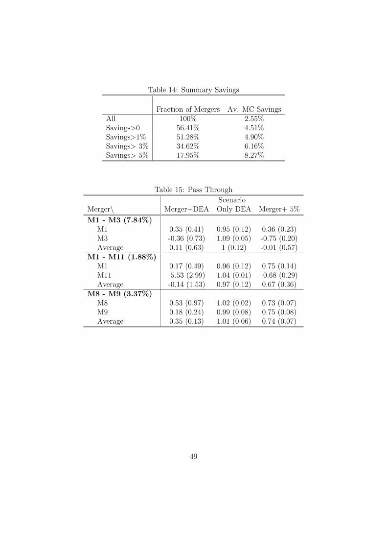
Table 14: Summary Savings

Fraction of Mergers Av. MC SavingsAll 100% 2.55%Savings>0 56.41% 4.51%Savings>1% 51.28% 4.90%Savings> 3% 34.62% 6.16%Savings> 5% 17.95% 8.27%

Table 15: Pass Through

ScenarioMerger\ Merger+DEA Only DEA Merger+ 5%

M1 - M3 (7.84%)M1 0.35 (0.41) 0.95 (0.12) 0.36 (0.23)M3 -0.36 (0.73) 1.09 (0.05) -0.75 (0.20)Average 0.11 (0.63) 1 (0.12) -0.01 (0.57)

M1 - M11 (1.88%)M1 0.17 (0.49) 0.96 (0.12) 0.75 (0.14)M11 -5.53 (2.99) 1.04 (0.01) -0.68 (0.29)Average -0.14 (1.53) 0.97 (0.12) 0.67 (0.36)

M8 - M9 (3.37%)M8 0.53 (0.97) 1.02 (0.02) 0.73 (0.07)M9 0.18 (0.24) 0.99 (0.08) 0.75 (0.08)Average 0.35 (0.13) 1.01 (0.06) 0.74 (0.07)

49

Table 16: Market Share VariationScenario

Merger\ Only Merger Merger+DEA Only DEA Merger+ 5%

M1 - M3 (7.84%)Outside 2.15% (0.23) -1.78% (0.20) -4.55 (0.42) -0.32 (0.07)Inside -9.12% (6.19) 6.93% (16.37) 19.37 (17.16) 0.14 (7.26)Average -3.35% (7.10) 2.48% (12.24) 7.13 (16.94) -0.1 (5.08)

M1 - M11 (1.88%)Outside 1.11% (0.09) 0.29% (0.04) -0.89% (0.07) -1.26% (0.11)Inside -2.65% (5.05) 1.28% (6.34) 4.13% (3.61) 7.71% (5.95)Average -0.19% (3.47) 0.63% (3.76) 0.85% (3.20) 1.85% (5.52)

M8 - M9 (3.37%)Outside 0.33% (0.04) -0.66 (0.08) -1.07 (0.13) -1.20 (0.16)Inside -4.04% (0.17) 6.90 (6.37) 11.92 (6.59) 14.16 (5.12)Average 0.17% (0.83) -0.38 (1.88) -0.59 (2.76) -0.63 (3.07)

Table 17: Profits by Firm

Manufacturers\Merger M1 - M3 M1 - M11 M8 - M9

Cost Savings 7.84% (0.36) 1.88% (0.18) 1.62 % (1.3)Manufacturer 1 17.39% 4.63% -0.71%Manufacturer 2 -1.72% 0.30% -0.69%Manufacturer 3 19.10% 0.31% -0.74%Manufacturer 4 -1.39% 0.27% -0.58%Manufacturer 5 -1.20% 0.25% -0.53%Manufacturer 6 -1.78% 0.30% -0.70%Manufacturer 7 -1.81% 0.30% -0.73%Manufacturer 8 -1.83% 0.30% 12.86%Manufacturer 9 -1.82% 0.30% 12.80%Manufacturer 10 -1.79% 0.30% -0.72%Manufacturer 11 -1.83% 2.00% -0.74%Manufacturer 12 -1.79% 0.30% -0.72%Manufacturer 13 -1.79% 0.30% -0.73%

50

References

Orley C. Ashenfelter, Daniel S. Hosken, and Matthew C. Weinberg. E�ciencies

brewed: pricing and consolidation in the US beer industry. RAND Journal of

Economics, 46(2):328–361, 2015.

Jonathan B. Baker and Timothy F. Bresnahan. The gains from merger

or collusion in product-di↵erentiated industries. The Journal of Industrial

Economics, 33(4):427–444, 1985.

Steven Berry and Ariel Pakes. Some applications and limitations of recent

advances in empirical industrial organization: Merger analysis. The American

Economic Review, 83(2):247–252, 1993.

Steven Berry, James Levinsohn, and Ariel Pakes. Automobile Prices in Market

Equilibrium. Econometrica, 63(4):841–890, 1995.

Steven T Berry. Estimating Discrete-Choice Models of Product Di↵erentiation.

The RAND Journal of Economics, 25(2):242–262, 1994.

Peter Bogetoft and Dexiang Wang. Estimating the Potential Gains from Mergers.

Journal of Productivity Analysis, 23(2):145–171, 2005.

Alessandro Bonanno. Functional foods as di↵erentiated products: the Italian

yogurt market. European Review of Agrcultural Economics, pages 1–27, 2012.

C. Bonnet and P. Dubois. Inference on vertical contracts between manufacturers

and retailers allowing for nonlinear pricing and resale price maintenance. RAND

Journal of Economics, 41(1):139–164, 2010.

51

C. Bonnet and V. Requillart. Impact of cost shocks on consumer price in

vertically-related markets: the case of the french soft drink market. American

Journal of Agricultural Economics, 95(5):1088–1108, 2013.

C. Bonnet, T. Corre, and V. Requillart. Price transmission in food chains: The

case of the dairy industry. Food Price Dynamics and Price Adjustment in the

EU edited by Steve McCorriston, Oxford University Press, 2015.

Timothy F Bresnahan. Empirical Studies of Industries with Market Power.

Handbook of Industrial Organization, II:1021–1957, 1989.

Adrian Brush, Eric Masanet, and Ernst Worrell. Energy E�ciency Improvement

and Cost Saving Opportunities for the Dairy Processing Industry. 2011.

O. Budzinski and Isabel Ruhmer. Merger simulation in competition policy: A

survey. Journal of Competition Law and Economics, 6(2):277–319, 2009.

William W. Cooper, Lawrence M Seiford, and Kaoru Tone. Introduction to Data

Envelopment Analysis and its Uses. Springer, 2005.

Michaela Draganska and Dipak C. Jain. Consumer Preferences and Product-Line

Pricing Strategies: An Empirical Analysis. Marketing Science, 25(2):164–174,

2006.

Ying Fan. Ownership Consolidation and Product Characteristics: A Study of the

US Daily Newspaper Market. American Economic r, 103(5):1598–1628, 2013.

Joseph Farrell and Carl Shapiro. Horizontal Mergers : An Equilibrium Analysis.

American Economic Review, 80(1):107–126, 1990.

52

Joseph Farrell and Carl Shapiro. Scale Economies and Synergies in Horizontal

Merger Analysis. Antitrust Law Journal, 68:685–710, 2001.

M. J. Farrell. The measurement of productive e�ciency. Journal of the Royal

Statistical Society. Series A (General), 120(3):253–290, 1957.

F. Gasmi, J.J. La↵ont, and Q. Vuong. Econometric analysis of collusive behavior

in a soft-drink market. Journal of Economics & Management Strategy, 12(1):

277–311, 1992.

Pinelopi K Goldberg. Product Di↵erentiation and Oligopoly in International

Markets: The Case of the U.S. Automobile Industry. Econometrica, 63(4):

891–951, 1995.

Klaus Gugler, Dennis C. Mueller, B. Burcin Yurtoglu, and Christine Zulehner.

The e↵ects of mergers: an international comparison. International Journal of

Industrial Organization, 21(5):625–653, 2003.

Jerry A. Hausman and Gregory K. Leonard. Using merger simulation models:

Testing the underlying assumptions. International Journal of Industrial

Organization, 23(9-10):693–698, 2005.

Marc Ivaldi and Frank Verboven. Quantifying the e↵ects from horizontal

mergers in European competition policy. International Journal of Industrial

Organization, 23(9-10):669–691, 2005.

Yong-bae Ji and Choonjoo Lee. Data envelopment analysis. The Stata Journal,

(2):267–280, 2010.

53

A. Kneip, L. Simar, and Paul W. Wilson. Asymptotics and consistent bootstraps

for dea estimators in nonparametric frontier models. Econometric Theory, 24:

1663–1697, 2008.

Michael Mazzeo, Mauricio Varela, and Katja Seim. The Welfare Consequences of

Mergers with Endogenous Product Choice. Working Paper, (August), 2014.

D. McFadden and K. Train. Mixed mnl models for discrete response. Journal of

applied Econometrics, 15(5):447–470, 2000.

Aviv Nevo. Identification of the oligopoly solution concept in a di↵erentiated-

products industry. Economics Letters, 59(3):391–395, 1998.

Aviv Nevo. Mergers with di↵erentiated products: The case of the ready-to-eat

cereal industry. The RAND Journal of Economics, 31(3):395–421, 2000.

Aviv Nevo. Measuring Market Power in the Ready-to-Eat Cereal Industry.

Econometrica, 69(2):307–342, 2001.

A. Petrin and K. Train. A control function approach to endogeneity in consumer

choice models. Journal of Marketing Research, 47(1):3–13, 2010.

P. Rey and T. Verge. Resale Price Maintenance and Interlocking Relationships.

Journal of Industrial Economics, 58(4):928961, 2010.

James N Rosse. Estimating cost function parameters without using cost data.

Econometrica, 38(2), 1970.

Margaret E. Slade. Market power and joint dominance in U.K. brewing. Journal

of Industrial Economics, 52(1):133–163, 2004.

54

J.V. Terza, A. Basu, and P.J. Rathouz. Two-stage residual inclusion estimation

addressing endogeneity in health econometric modeling. Journal of Health

Economics, 27(3):531–543, 2008.

Frank Verboven. International Price Discrimination in the European Car Market.

RAND Journal of Economics, 27(2):240–268, 1996.

Sofia Berto Villas-Boas. Vertical relationships between manufacturers and

retailers: Inference with limited data. Review of Economic Studies, 74(2):

625–632, 2007.

Gregory J. Werden and Luke M. Froeb. The e↵ects of mergers in di↵erentiated

products industries: Logit demand and merger policy. Journal of Law,

Economics, & Organization, 10(2):407–426, 1994.

Gregory J. Werden and Luke M. Froeb. The Economics of the Antitrust Process.

Kluwer Academic Publishers, 1996.

55

PREVIOUS DISCUSSION PAPERS

244 Bonnet, Céline and Schain, Jan Philip, An Empirical Analysis of Mergers: Efficiency Gains and Impact on Consumer Prices, February 2017.

243 Benndorf, Volker and Martinez-Martinez, Ismael, Perturbed Best Response Dynamics in a Hawk-Dove Game, January 2017.

242 Dauth, Wolfgang, Findeisen, Sebastian and Suedekum, Jens, Trade and Manufacturing Jobs in Germany, January 2017. Forthcoming in: American Economic Review, Papers & Proceedings.

241 Borrs, Linda and Knauth, Florian, The Impact of Trade and Technology on Wage Components, December 2016.

240 Haucap, Justus, Heimeshoff, Ulrich and Siekmann, Manuel, Selling Gasoline as a By-Product: The Impact of Market Structure on Local Prices, December 2016.

239 Herr, Annika and Normann, Hans-Theo, How Much Priority Bonus Should be Given to Registered Organ Donors? An Experimental Analysis, November 2016.

238 Steffen, Nico, Optimal Tariffs and Firm Technology Choice: An Environmental Approach, November 2016.

237 Behrens, Kristian, Mion, Giordano, Murata, Yasusada and Suedekum, Jens, Distorted Monopolistic Competition, November 2016.

236 Beckmann, Klaus, Dewenter, Ralf and Thomas, Tobias, Can News Draw Blood? The Impact of Media Coverage on the Number and Severity of Terror Attacks, November 2016. Forthcoming in: Peace Economics, Peace Science and Public Policy.

235 Dewenter, Ralf, Dulleck, Uwe and Thomas, Tobias, Does the 4th Estate Deliver? Towars a More Direct Measure of Political Media Bias, November 2016.

234 Egger, Hartmut, Kreickemeier, Udo, Moser, Christoph and Wrona, Jens, Offshoring and Job Polarisation Between Firms, November 2016.

233 Moellers, Claudia, Stühmeier, Torben and Wenzel, Tobias, Search Costs in Concentrated Markets – An Experimental Analysis, October 2016.

232 Moellers, Claudia, Reputation and Foreclosure with Vertical Integration – Experimental Evidence, October 2016.

231 Alipranti, Maria, Mitrokostas, Evangelos and Petrakis, Emmanuel, Non-comparative and Comparative Advertising in Oligopolistic Markets, October 2016. Forthcoming in: The Manchester School.

230 Jeitschko, Thomas D., Liu, Ting and Wang, Tao, Information Acquisition, Signaling and Learning in Duopoly, October 2016.

229 Stiebale, Joel and Vencappa, Dev, Acquisitions, Markups, Efficiency, and Product Quality: Evidende from India, October 2016.

228 Dewenter, Ralf and Heimeshoff, Ulrich, Predicting Advertising Volumes: A Structural Time Series Approach, October 2016.

227 Wagner, Valentin, Seeking Risk or Answering Smart? Framing in Elementary Schools, October 2016.

226 Moellers, Claudia, Normann, Hans-Theo and Snyder, Christopher M., Communication in Vertical Markets: Experimental Evidence, July 2016. Published in: International Journal of Industrial Organization, 50 (2017), pp. 214-258.

225 Argentesi, Elena, Buccirossi, Paolo, Cervone, Roberto, Duso, Tomaso and Marrazzo, Alessia, The Effect of Retail Mergers on Prices and Variety: An Ex-post Evaluation, June 2016.

224 Aghadadashli, Hamid, Dertwinkel-Kalt, Markus and Wey, Christian, The Nash Bargaining Solution in Vertical Relations With Linear Input Prices, June 2016. Published in: Economics Letters, 145 (2016), pp. 291-294.

223 Fan, Ying, Kühn, Kai-Uwe and Lafontaine, Francine, Financial Constraints and Moral Hazard: The Case of Franchising, June 2016. Forthcoming in: Journal of Political Economy.

222 Benndorf, Volker, Martinez-Martinez, Ismael and Normann, Hans-Theo, Equilibrium Selection with Coupled Populations in Hawk-Dove Games: Theory and Experiment in Continuous Time, June 2016. Published in: Journal of Economic Theory, 165 (2016), pp. 472-486.

221 Lange, Mirjam R. J. and Saric, Amela, Substitution between Fixed, Mobile, and Voice over IP Telephony – Evidence from the European Union, May 2016. Published in: Telecommunications Policy, 40 (2016), pp. 1007-1019.

220 Dewenter, Ralf, Heimeshoff, Ulrich and Lüth, Hendrik, The Impact of the Market Transparency Unit for Fuels on Gasoline Prices in Germany, May 2016. Published in: Applied Economics Letters, 24 (2017), pp. 302-305.

219 Schain, Jan Philip and Stiebale, Joel, Innovation, Institutional Ownership, and Financial Constraints, April 2016.

218 Haucap, Justus and Stiebale, Joel, How Mergers Affect Innovation: Theory and Evidence from the Pharmaceutical Industry, April 2016.

217 Dertwinkel-Kalt, Markus and Wey, Christian, Evidence Production in Merger Control: The Role of Remedies, March 2016.

216 Dertwinkel-Kalt, Markus, Köhler, Katrin, Lange, Mirjam R. J. and Wenzel, Tobias, Demand Shifts Due to Salience Effects: Experimental Evidence, March 2016. Forthcoming in: Journal of the European Economic Association.

215 Dewenter, Ralf, Heimeshoff, Ulrich and Thomas, Tobias, Media Coverage and Car Manufacturers’ Sales, March 2016. Published in: Economics Bulletin, 36 (2016), pp. 976-982.

214 Dertwinkel-Kalt, Markus and Riener, Gerhard, A First Test of Focusing Theory, February 2016.

213 Heinz, Matthias, Normann, Hans-Theo and Rau, Holger A., How Competitiveness May Cause a Gender Wage Gap: Experimental Evidence, February 2016. Forthcoming in: European Economic Review, 90 (2016), pp. 336-349.

212 Fudickar, Roman, Hottenrott, Hanna and Lawson, Cornelia, What’s the Price of Consulting? Effects of Public and Private Sector Consulting on Academic Research, February 2016.

211 Stühmeier, Torben, Competition and Corporate Control in Partial Ownership Acquisitions, February 2016. Published in: Journal of Industry, Competition and Trade, 16 (2016), pp. 297-308.

210 Muck, Johannes, Tariff-Mediated Network Effects with Incompletely Informed Consumers, January 2016.

209 Dertwinkel-Kalt, Markus and Wey, Christian, Structural Remedies as a Signalling Device, January 2016. Published in: Information Economics and Policy, 35 (2016), pp. 1-6.

208 Herr, Annika and Hottenrott, Hanna, Higher Prices, Higher Quality? Evidence From German Nursing Homes, January 2016. Published in: Health Policy, 120 (2016), pp. 179-189.

207 Gaudin, Germain and Mantzari, Despoina, Margin Squeeze: An Above-Cost Predatory Pricing Approach, January 2016. Published in: Journal of Competition Law & Economics, 12 (2016), pp. 151-179.

206 Hottenrott, Hanna, Rexhäuser, Sascha and Veugelers, Reinhilde, Organisational Change and the Productivity Effects of Green Technology Adoption, January 2016. Published in: Energy and Ressource Economics, 43 (2016), pp. 172–194.

205 Dauth, Wolfgang, Findeisen, Sebastian and Suedekum, Jens, Adjusting to Globa-lization – Evidence from Worker-Establishment Matches in Germany, January 2016.

204 Banerjee, Debosree, Ibañez, Marcela, Riener, Gerhard and Wollni, Meike, Volunteering to Take on Power: Experimental Evidence from Matrilineal and Patriarchal Societies in India, November 2015.

203 Wagner, Valentin and Riener, Gerhard, Peers or Parents? On Non-Monetary Incentives in Schools, November 2015.

202 Gaudin, Germain, Pass-Through, Vertical Contracts, and Bargains, November 2015. Published in: Economics Letters, 139 (2016), pp. 1-4.

201 Demeulemeester, Sarah and Hottenrott, Hanna, R&D Subsidies and Firms’ Cost of Debt, November 2015.

200 Kreickemeier, Udo and Wrona, Jens, Two-Way Migration Between Similar Countries, October 2015. Forthcoming in: World Economy.

199 Haucap, Justus and Stühmeier, Torben, Competition and Antitrust in Internet Markets, October 2015. Published in: Bauer, J. and M. Latzer (Eds.), Handbook on the Economics of the Internet, Edward Elgar: Cheltenham 2016, pp. 183-210.

198 Alipranti, Maria, Milliou, Chrysovalantou and Petrakis, Emmanuel, On Vertical Relations and the Timing of Technology, October 2015. Published in: Journal of Economic Behavior and Organization, 120 (2015), pp. 117-129.

197 Kellner, Christian, Reinstein, David and Riener, Gerhard, Stochastic Income and Conditional Generosity, October 2015.

196 Chlaß, Nadine and Riener, Gerhard, Lying, Spying, Sabotaging: Procedures and Consequences, September 2015.

195 Gaudin, Germain, Vertical Bargaining and Retail Competition: What Drives Countervailing Power? September 2015.

194 Baumann, Florian and Friehe, Tim, Learning-by-Doing in Torts: Liability and Information About Accident Technology, September 2015.

193 Defever, Fabrice, Fischer, Christian and Suedekum, Jens, Relational Contracts and Supplier Turnover in the Global Economy, August 2015. Published in: Journal of International Economics, 103 (2016), pp. 147-165.

192 Gu, Yiquan and Wenzel, Tobias, Putting on a Tight Leash and Levelling Playing Field: An Experiment in Strategic Obfuscation and Consumer Protection, July 2015. Published in: International Journal of Industrial Organization, 42 (2015), pp. 120-128.

191 Ciani, Andrea and Bartoli, Francesca, Export Quality Upgrading under Credit

Constraints, July 2015. 190 Hasnas, Irina and Wey, Christian, Full Versus Partial Collusion among Brands and

Private Label Producers, July 2015.

189 Dertwinkel-Kalt, Markus and Köster, Mats, Violations of First-Order Stochastic Dominance as Salience Effects, June 2015. Published in: Journal of Behavioral and Experimental Economics, 59 (2015), pp. 42-46.

188 Kholodilin, Konstantin, Kolmer, Christian, Thomas, Tobias and Ulbricht, Dirk, Asymmetric Perceptions of the Economy: Media, Firms, Consumers, and Experts, June 2015.

187 Dertwinkel-Kalt, Markus and Wey, Christian, Merger Remedies in Oligopoly under a Consumer Welfare Standard, June 2015 Published in: Journal of Law, Economics, & Organization, 32 (2016), pp. 150-179.

186 Dertwinkel-Kalt, Markus, Salience and Health Campaigns, May 2015 Published in: Forum for Health Economics & Policy, 19 (2016), pp. 1-22.

185 Wrona, Jens, Border Effects without Borders: What Divides Japan’s Internal Trade? May 2015.

184 Amess, Kevin, Stiebale, Joel and Wright, Mike, The Impact of Private Equity on Firms’ Innovation Activity, April 2015. Published in: European Economic Review, 86 (2016), pp. 147-160.

183 Ibañez, Marcela, Rai, Ashok and Riener, Gerhard, Sorting Through Affirmative Action: Three Field Experiments in Colombia, April 2015.

182 Baumann, Florian, Friehe, Tim and Rasch, Alexander, The Influence of Product Liability on Vertical Product Differentiation, April 2015. Published in: Economics Letters, 147 (2016), pp. 55-58 under the title “Why Product Liability May Lower Product Safety”.

181 Baumann, Florian and Friehe, Tim, Proof beyond a Reasonable Doubt: Laboratory Evidence, March 2015.

180 Rasch, Alexander and Waibel, Christian, What Drives Fraud in a Credence Goods Market? – Evidence from a Field Study, March 2015.

179 Jeitschko, Thomas D., Incongruities of Real and Intellectual Property: Economic Concerns in Patent Policy and Practice, February 2015. Forthcoming in: Michigan State Law Review.

178 Buchwald, Achim and Hottenrott, Hanna, Women on the Board and Executive Duration – Evidence for European Listed Firms, February 2015.

177 Heblich, Stephan, Lameli, Alfred and Riener, Gerhard, Regional Accents on Individual Economic Behavior: A Lab Experiment on Linguistic Performance, Cognitive Ratings and Economic Decisions, February 2015 Published in: PLoS ONE, 10 (2015), e0113475.

176 Herr, Annika, Nguyen, Thu-Van and Schmitz, Hendrik, Does Quality Disclosure Improve Quality? Responses to the Introduction of Nursing Home Report Cards in Germany, February 2015. Published in: Health Policy, 120 (2016), pp.1162-1170.

175 Herr, Annika and Normann, Hans-Theo, Organ Donation in the Lab: Preferences and Votes on the Priority Rule, February 2015. Published in: Journal of Economic Behavior and Organization, 131 Part B (2016), pp. 139-149.

174 Buchwald, Achim, Competition, Outside Directors and Executive Turnover: Implications for Corporate Governance in the EU, February 2015.

173 Buchwald, Achim and Thorwarth, Susanne, Outside Directors on the Board, Competition and Innovation, February 2015.

172 Dewenter, Ralf and Giessing, Leonie, The Effects of Elite Sports Participation on Later Job Success, February 2015.

171 Haucap, Justus, Heimeshoff, Ulrich and Siekmann, Manuel, Price Dispersion and Station Heterogeneity on German Retail Gasoline Markets, January 2015. Forthcoming in: The Energy Journal.

170 Schweinberger, Albert G. and Suedekum, Jens, De-Industrialisation and Entrepreneurship under Monopolistic Competition, January 2015 Published in: Oxford Economic Papers, 67 (2015), pp. 1174-1185.

Older discussion papers can be found online at:

http://ideas.repec.org/s/zbw/dicedp.html

ISSN 2190-9938 (online) ISBN 978-3-86304-243-1