an efficient method for nonlinear analysis of layered shells

Sddhand, Vol. 25, Part 4, August 2000, pp. 381-408. ,(", Printed in India

An efficient method for nonlinear analysis of layered shells

W P P R E M A K U M A R 1 and R P A L A N I N A T H A N 2

1Department of Civil Engineering, JNN College of Engineering, Shimoga 577 204, India 2Department of Applied Mechanics, Indian Institute of Technology Madras, Chennai 600036, India. e-mail: rpnathan @ iitm.ernet.in

Abstract. Finite element formulation based on explicit through-thickness • integration scheme assumes importance when applied to multilayered shells, as it is numerically accurate and computationally efficient. Explicit integration becomes possible on assuming the variation of the inverse Jacobian through the thickness. The element stiffness matrices are discussed for (i) large rotation, and (ii) small rotation. Relative efficiencies of the explicit through- thickness integration schemes are compared with that of the conventional formulation involving numerical integration in three directions in each layer and summation over the layers. The small rotation formulation assuming linear variation of the Jacobian inverse across the thickness and based on further approximation regarding certain submatrices is seen to be computationally efficient. The geometric nonlinear behaviours of laminated composite cylindrical panels subjected to external pressure are discussed. The parameters considered are: number of layers, symmetric/antisymmetric, cross-ply/angle- ply, boundary conditions and central angle. The strength of shallow panels with longitudinal edges hinged and curved edges free is controlled by the limit point load, while for deep panels it is controlled by the bifurcation load. The boundary conditions have significant influence on load carrying capacities.

Keywords. Geometric nonlinear finite element analysis; layered shells; explicit through-thickness integration scheme; numerical accuracy; computational efficiency.

1. Introduction

Structures made of fibre reinforced composite materials have necessarily to be of layered construction with different fibre orientations in order to exploit the direction-dependent properties of the basic lamina. The analyst has to deal with a larger number of elastic

A list of symbols is given at the end of the paper

381

382 W P Prema Kumar and R Palaninathan

constants and, further, layered construction results in various types of coupling in structural behaviour such as stretching-shear, stretching-bending etc. (Vinson & Sierakowski 1986). Coupled behaviour leads to complexity in the analysis and prediction of load-carrying capacities.

Composite shells are generally very thin and hence their load carrying capacities are usually controlled by their buckling strengths. Classical buckling strength calculation is based on the assumption of negligible pre-buckling deformations and the buckling is characterized by a sudden out-of-plane displacement, during which there is an exchange of energy from membrane state to bending state. This assumption is not strictly valid in the case of layered shells. Due to bending-stretching coupling, there is considerable out-of- plane displacement even for very small in-plane loads. In view of this characteristic behaviour, the buckling analysis of laminated structures cannot be treated as an eigenvalue problem. Nonlinear analysis is seen to be appropriate for determining the strengths of layered composite shell structures. Fibre reinforced composite materials exhibit linear stress-strain behaviour up to failure. Layered shells made of composite materials, being very thin, undergo large deformations and hence geometric nonlinear analysis assumes importance.

In view of the complexities associated with layered composite shell structures, the finite element method of solution is the natural choice for analysis. In the conventional formulation of degenerated shell elements (Ahmad et al 1970; Surana 1983), 3-D numerical integration is carried out to compute the element matrices. The direct exten- sion of the same to the layered shells (Panda & Natarajan 1981) becomes computationally inefficient when the number of layers in the laminate is large, which is usually the case in reality. In order to overcome this, explicit through-thickness integration schemes (Yunus et al 1989; Vlachoutsis 1990) have been formulated for linear problems. Explicit integration through the thickness becomes possible when the elements of the inverse Jacobian are assumed to either remain constant or have a particular variation through thickness. Three such models have been evaluated from the points of view of numerical accuracy and computational efficiency for linear stress analysis and classical buckling (Prema Kumar & Palaninathan 1997). In the present paper, the formulations for geometric nonlinear problems of laminated shells based on explicit through-thickness integration are discussed. Equations are presented for both large rotation and small rotation cases. The computational scheme which involves numerical integration in the three directions in each layer and then summation over the layers is designated the NI Model. The other schemes involve explicit through-thickness integration based on assumed variation of the elements of the Jacobian inverse matrix across the thickness. "The scheme which assumes that the elements of the Jacobian inverse vary linearly across the thickness is designated the EI-1 Model and that which assumes constant Jacobian inverse is designated the EI-2 Model. The EI-3 Model is a modification of the EI-1 Model in which certain submatrices whose elements have negligible magnitude (higher order terms of thickness coordinate) are dropped with a view to improving the computational efficiency. Numerical accuracies and computational efficiencies of the explicit through-thickness integration models have been discussed by comparing them with those of the NI Model with respect to geometrically nonlinear problems. The EI-3 Model under the small rotation scheme is found to be adequate for laminated shells with no significant sacrifice of numerical accuracy due to the simplifying assumptions. The results of a parametric study of externally pressurized layered cylindrical panels using the EI-3 Model are presented and discussed.

An efficient method for nonlinear analysis of layered shells 383

2. Element formulations

The element employed in the present work is a 8-node degenerated curved shell element (parabolic) which is shown in figure 1. The degrees of freedom at a node n are u,, v,, w,, C~n and/3,. The layers are assumed to be perfectly bonded to one another and transversely isotropic. Serendipity shape functions (Zienkiewicz 1977) are used. The formulations for geometric nonlinear analysis are based on total Lagrangian description with Zienkiewicz's B-notation. First, the large rotation formulation for layered shells (NI Model) is presented. Next, the explicit through-thickness integration schemes (Models EI-1 through EI-3) are presented. Finally, by specialization, small rotation formulations are obtained.

2.1 Large rotation formulations (LRF) for layered shells

2.1a NI model: The conventional formulation which involves numerical integration in three directions in each layer and summation over the layers is termed the NI Model. The displacement field at any point (~,~,~) within the element (Panda & Natarajan 1981; Surana 1983) is given by

{!}, {/+ un " F,~ = ~ N . ( ~ , , 7 ) v. + Z N . ( ~ , , 7 ) ~ F.v ,

, = , w. ~ .:, t F.+z ) (la)

Z

~Lr_.v x ~ : -1 nbot middle surface

Global axes (a)

Node n x.J 13 n Vln

t/2

t / 2

+ '

P 3 ""

(b) (c)

Figure 1. Eight-node layered shell element.

384

where

W P Prema Kumar and R Palaninathan

hk = a~ +-~- ~k, (lb)

t h~ k ak-- 2 2 + E hi. (lc)

i=1

Nonlinear functions of nodal rotations are given by

Fny = ~sinc~.(1 ~-COSt~n)]Vlnv( --~ (COS OZ n "t- 1) s in /3n g2ny f rnz t VnzJ V2nzJ

+ (cos c~. cos ~. - 1) ) V3.y tV , . z

(2)

Applying the principle of virtual work, taking variation of residual force with respect to nodal displacements, {d} and making mathematical transformations, we have (Surana 1983)

[k T] = [k O] -{-[k LI ] + [k L2] q - [ k crl ] q - [ k cr2] Jr-[kcr3], ( 3 )

where

where

.L / , /_ , f hk [ k°] = ~ [B°]r [Elk [ B°] IJI t d~k dr/d~, (4) k=l 1 1 1

i l/_' i' [~'] = ~ [n°lr[e]~[sq IJ1-7- k=l 1 1 1

k=l 1 1 1

[kLZ] = ~ [8~] r [e]k [B L] Ial S- d¢~ 0,7 de (6) k=l 1 1 l

[k<] = ~ [G] r [s] [G]IJI t dsc dr/dO, (7) k=l 1 1 1

(5)

[B °] = [/4] [6], [B L] = [A] [6],

[S]-- [ o-x[/,].

/ Symmetric

~ . [t,] ~-x~ [1,] o.y [I3] ry: [I3]

0-:[13]

(8) (9)

(10)


For the initial stress matrices, [k a2] and [kCr3], the reader is referred to the thesis by Prema Kumar (1996). The effects of the nonlinear functions of rotations appear in the tangent stiffness matrix in the form of initial stress matrices [k ~2] and [k ~3] . In the above formulation, the matrix [k °] is a function of {d} because of large rotation. It is constant in the small rotation formulation.

The internal force vector is given by

{F e} = fv[B]T{cr} dV = [kS]{d},

where [k s] = secant stiffness matrix of the element, is given by

k~l /1 fl / 1 hk [kS] = 1 1 , [o]r[E]k[B] lJ I y d~k d~/d~,

where

(11)

(12)

(14)

(14a)

(14b)

(14c)

(14d)

vary linearly across the shell thickness, i.e.,

J* = S a + (2/t)~S~.

Let the determinant of the Jacobian matrix be [J[ and let

At = ~ / ~ , at the top of the shell surface,

Ab = V / ~ , at the bottom of the shell surface,

= ½ + xb),

[/~] = [B °] + ½ [B L] is the total strain-displacement matrix. (13)

As seen from (4) through (7), the element matrices are computed using 3-D numerical integration in each layer and summing over layers. It is obvious that the computational time for these element matrices increases linearly with the number of layers (NL).For the case of a laminate with a large number of layers, it proves to be computationally expensive. The integrands of the above equations are complicated functions of {, ~/and 4- The integrands are products of three kinds of terms. [E]~ is a material property matrix which is constant for each layer but varies from layer to layer either due to change in fibre orientation or change in material. This term does not give rise to any complication with regard to the integration. While the variation of the incremental strain-displacement matrix [B] with respect to { and ~/is quite complex, its variation with respect to the thickness coordinate, ~, can be modelled by simple functions, particularly for thin shells. The same is true for the third term in the integrand, namely the determinant of the Jacobian. The variations of both these terms are controlled by the Jacobian inverse [J*]. While the variation of [J*] in the tangential plane ({, ~/) is quite complex, the variation of the same in the thickness direction can be modelled by simple functions that are linear or constant for thin shells. Such assumptions will lead to the explicit integration of through-thickness effects and numerical integration in the tangential plane ({, ~7) of the middle surface irrespective of the number of layers in the laminate. It is quite obvious that this approach will result in considerable saving in computational time.

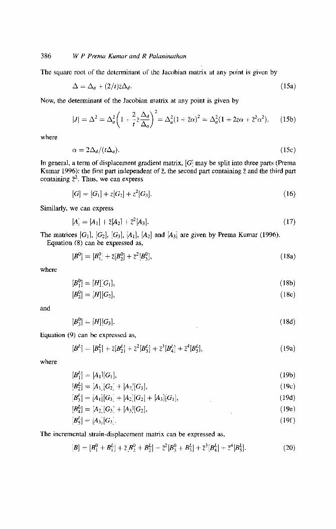
2.1b EL1 model: This model assumes that the elements of the Jacobian inverse matrix


The square root of the determinant of the Jacobian matrix at any point is given by

A = A a + (2 / t ) 2A d. (15a)

Now, the determinant of the Jacobian matrix at any point is given by

2- Ad'~ 2 I J I = A 2 = A 2 l + t z - z - ll..xa,/ =A2(1ff-ZOl)2=A2(lq'-2Z.Olq-22O12), (15b)

where

ol = 2 A d / ( t A a ) . (15c)

In general, a term of displacement gradient matrix, [G] may be split into three parts (Prema Kumar 1996): the first part independent of 2, the second part containing 2 and the third part containing 22 . Thus, we can express

[G] ~-- [G1] q- 2[G2] -}- 22[G3]. (16)

Similarly, we can express

[a] = [al] + 2[A2] + z2[a3]. (17)

The matrices [G1], [G2], [G3], [A1], [A2] and [A3] are given by Prema Kumar (1996). Equation (8) can be expressed as,

[B °] = [B °] + 2[B °] + 22[B°], (18a)

where

and

[B °] = [H][G,], (18b)

[B2 °] = [H] [G2], (18c)

[B °] = [H][Z3].

Equation (9) can he expressed as,

[O L] = [B1 L] q- z[B L] q- z2[B3 L] q- 23[B L] q-- 24[BL],

where

[B1 ~] =[AI] [C~], [B L] = [AI][G2] q--- [A2][GI] ,

IBm] = [A,][~] + [A~][C~] + [A~][Cl], [B4 L] = [A2] [G3] + [A3] [G2],

[S L] : [A3][G3].

The incremental strain-displacement matrix can be expressed as,

. T-4 fRLI [B] : [B10 q-Bl L] +z[B2 0 q-B L] q-z2[B°-]-B~] q-z3[B4L ] q-,~ t~5].

(18d)

(19a)

(19b)

(19c)

(19d)

(19e)

(19f)

(20)


Equation (13) can be expressed as,

[[t]=[B°+½BL]+2[ B°+IL~B2] if- z2[ BO+IBL]2 3 q- z3[½ BL] q- ~4[½BL]. (21)

In (18) and (19). the matrices [B °] through [B °] and [B L] through [B L] are independent of and thus through-thickness integration becomes possible. Substitution of (15b) and (18a) into (4), and taking the thickness integration in each layer and layer summation inside the integrand, results in integration over the middle surface alone as,

[k O] -~- [[B°]T[EI][B°I] -~- [B°]T[E2][B O] + [B°I]T[E3][B O] + [B°2]T[E2][B O] 1 1

+ [B°]r[E3][B °] + [B°]r[E4][B °] + [B°]r[E3][B °] 2 + [B°3]T[E4][B°] + [B°]r[Es][B°3]] A2 t d~/d~. (22)

Substitution of (15b), (18a) and (i9a) into (5), and taking the thickness integration in each layer and layer summation inside the integrand, results in integration over the middle surface alone as,

f f [k Ll] = [[B°]r[E,][BIf] + [B°]r[E2][B~] + [B°]T[E3][BI~] + [B°]r[E4][B~] 1 1

q- [B?jT [E5][BI~] if-[B°]T[E2J[B L] q-[B°]TfE3J[B L] --~ [n°lT [E4J[g L] q- [B°]T [E5][B L] q-[n°]T[fe][n L] q-[n°3]T[E3][n L] q-- [B°]T [E4][B L] + [B°]r[EsJ[B~] + [B°]r[E6][BI2] + [B°]r[E7][B~] + [Btf]r[E1][B °]

+ [BLI]r[E2][B°] + [Btf]r[E3][B °] + [B~]r[E2][B °] + [B~]r[E3][B °] q- [BL]T [E4][B O] q-[BL]T[E3][B?] Jr-[BL]T[E4][B O] -Jr [B~]T [E5][B O] + [BL]T[E4J[B °] + [BL]r[Es][B °] + [BL]r[E6][B °] + [BI~JT[Es][B°I]

2 dr/d~, (23) + [BL]T[E6J[BO]-[-[BL]T[E7][BOJ]A2a t

where

NL [Eli = Z [ E ] k ( ( v a r 1 ) + 2c~(var 2) + c~2(var 3))k,

k=l NL

[E2] = Z [ E ] k ( ( v a r 2) + 2a(var 3) + ol2(var4))k, k=l NL

[E3] = Z [ E ] k ( ( v a r 3 ) + 2cffvar4) + c~2(var5))k, k=l

vat 1 = (~t - z+) = h, 1

= - z ~ ) , var 2 ~ (zt -~

1 var3 =


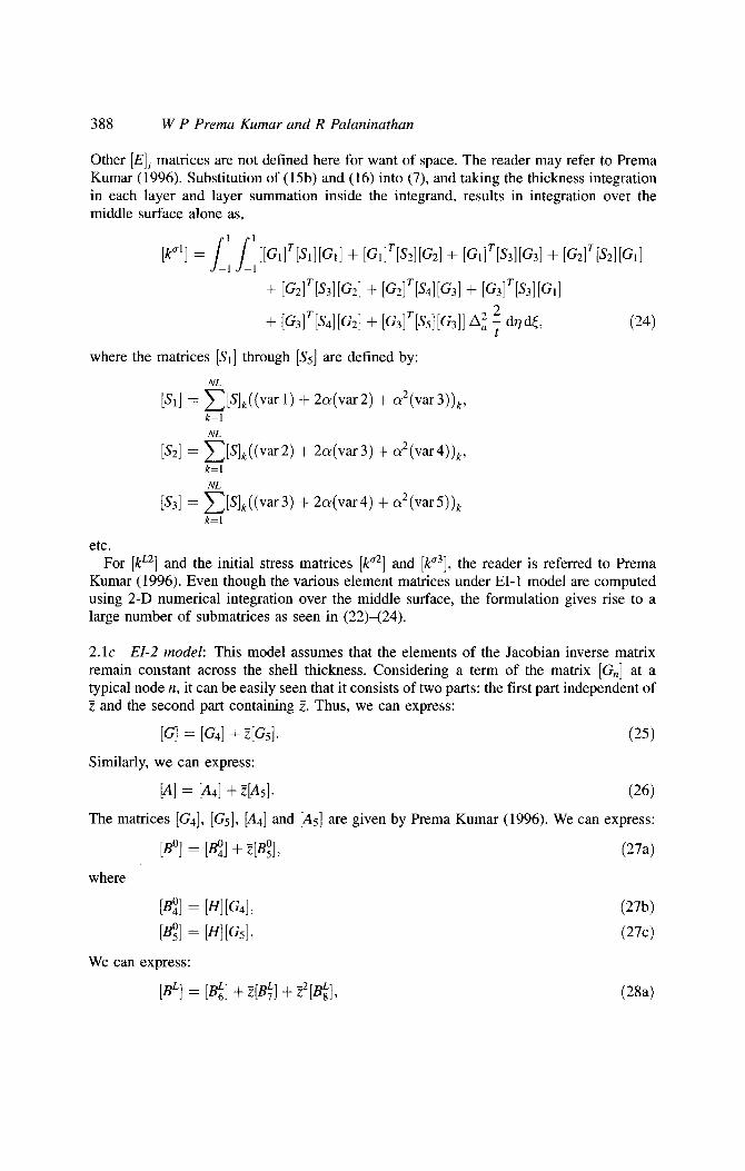
Other [E]i matrices are not defined here for want of space. The reader may refer to Prema Kumar (1996). Substitution of (15b) and (16) into (7), and taking the thickness integration in each layer and layer summation inside the integrand, results in integration over the middle surface alone as, f/1

[k 41] =- [[G1]T[s,][G,] -k [G1]T[s2][G2] + [GI]T[Sa][G3] q-[G2]r[S2][GI] 1 1

+ [G2]T[S3][G2] + [G2]T[s4I[G3] + [G3]T[s3][G,] 2

-t-[G3IT[s4] [G2] ~- [G3]T[s5J[G3]] A 2 7 d~Td{, (24)

where the matrices [S,] through [$5] are defined by:

NL

[S1] = Z[S]k( (var 1 ) + 2c~(var 2 ) + o~2(var 3))k, k=l NL

[$21 = Z[S]k( (var 2 ) + 2a(var 3 ) + a2(var4))~, k=l NL

[$3] = Z[S]k( (var 3) + 2oe(var4) + c~2(var5))~ k=l

etc. For [k t'2] and the initial stress matrices [k "2] and [k'3], the reader is referred to Prema

Kumar (1996). Even though the various element matrices under EI-1 model are computed using 2-D numerical integration over the middle surface, the formulation gives rise to a large number of submatrices as seen in (22)-(24).

2.1c EI-2 model: This model assumes that the elements of the Jacobian inverse matrix remain constant across the shell thickness. Considering a term of the matrix [Gn] at a typical node n, it can be easily seen that it consists of two parts: the first part independent of

and the second part containing L Thus, we can express:

[G] = [G4] q- z[G5]. (25)

Similarly, we can express:

[Z] = [a4] + z[as]. (26)

The matrices [G4], [G5], [A4] and [As] are given by Prema Kumar (1996). We can express:

where

[B °] = [B °] + ~[B°], (27a)

[B 0] = [H][G4], (27b)

[B °] = [H] [G5]. (27c)

We can express:

[B L] = [B6 ~] + e[B~] + e2[B~], (28a)

where


[B L] = [A4][G4] ,

[B7 L] = [A4] [G5]- } - [A5] [G4],

We can express:

[8] = [8 0 + 8~1 + ~[8 ° + 8~] + ~[8~] ,

[j~] [B4 0 1 L z [B 0 1 L ~,2[1BL]. = q- ~n6] -]'- Jr- ~n7] -]-

389

(28b)

(28c)

(28d)

(29)

(30)

In (29) and (30), the matrices [B°], [B°], [B~] through [B~] are independent of ~ and thus through-thickness integration becomes possible. Substitution of (27a) into (4) and taking the thickness integration in each layer and the layer summation inside the integrand results in integration over the middle surface alone as:

[k °] = [[B°4]r[E,,][B°4] + [B°Jr[E12][B °] + [B°JT[EI2][B O] 1 1

+ [ns°]r [E,3] [B°]] I1107 d~. (31)

Substitution of (27a) and (28a) into (5) and taking the thickness integration in each layer and the layer summation inside the integrand results in integration over the middle surface alone as:

?/' [kL1] = [[B°]r[EI,][B L] + [B°]r[E,2][B L] + [B°Jr[e,3][B L] + [B°]T[E,2][B L] I 1

+ [B°]T[E13][B~] + [B°JT[E14]fB~] + [Bld]T[E,,][B °]

Jr-[BLjTfE12JfB05] "t- [Bf]T [E12] [B04] Jr-[BLIT[E13I[BO5J

+ [B8 L] r [E,3] In ° ] + [n~] r [El4] [B°]] I1107 d~. (32)

The matrices JEll] through [E15] are defined by:

NL [e, ,] = ~ [e]k(~, - ~b)k,

k=l l NL

1 NL [El3] = ~ [g]k( ~3 -- Z';)k'

l NL [E,4] = ~ ~ [E]k(2 ~ - 24) k,

l k~ ' ~5)


where

k k-I t h t

Zt=-- '2-} - Z "j' Zb=- -2 -~ - Z hj" j=l j=l

Substitution of (25) into (7) and taking the thickness integration in each layer and the layer summation inside the integrand results in integration over the middle surface alone as: f/1

[k ~rl] = [[G4]T[s6][G4] -I- [G4]T[s7][G5] + [G5]T[s7][G4] 1 1

+ [as]r [58] [65]] I11 d,7 04 (33)

where the matrices [$6] through [$8] are defined by:

NL [$61 ----- ~ [S]k(-Zt- Zb)k,

k=l 1NL

[sT] = ~ ~ [s]~(e~ - ~2)~,

1 NL [s+] = ~ ~ [s]~(~ - ~)k.

Comparing (22)-(24) with (31)-(33) respectively, it may be seen that the number of submatrices involved in the computation of various element matrices are considerably less in the EI-2 model. In other words, the EI-2 model is computationally efficient. However, its numerical accuracy needs to be ascertained.

2.1d EI-3 model: This model is obtained from the EI-1 model by dropping some submatrices of the EI-1 model whose elements are seen to be of very small magnitude. This is expected to result in computational efficiency. [G3] in (16) is one such matrix. After dropping [G3], (16) becomes:

[G] = [G,] + ~[G2]. (34)

Similarly, referring to (17) for EI-1 model and dropping the matrix [A3], we have:

[a] = [All + ~[a2]. (35)

As a result of the dropping of the matrices [G3] and [A3], the expressions for the key matrices for EI-3 model become:

[B °] = [B °] + E[B°],

[B L] = [B L] + ~.[B2 c] + 7.2 [O~],

Is] = [8 ° + 8~] + e[~ ° + 82q + ~2[@, [B] := [8 0 -t- bSD1]" IoL] _]_ ~[B 0 _]_ 1 B L] Jr- ~2[/B~].

(36)

(37)

(3s) (39)


Equation (22) reduces to:

[k o] = [[B°]~[e,] [B °] + [B°]~[e~] [B ° ] + [B°]~[e~] [B °] 1 1

2 + [B°]r[E3][B°]] AZa t dr/d¢ (40)

Equation (23) reduces to: /1/ [~'] = [[B°]~[e,][@ + [B°]~[e~][B~] + [Bl°]~[e~][B~] + [B°]~[e~l[B: ~]

I 1

+ [B°]r[E3][B L] + [B°]T[E4][BIf] + [BL]T[EI][B °]

+ [BL] r [E2][B °] + [BL]T[E2][B °] + [BL]r[E3][B °] 2 -]-[BL]T[E3I[B°I] + [BL]T [E4][B°2]] A2a 7 dT/d¢. (41)

Equation (24) reduces to: //1 [k 'r'] = [[G1]T[sI][G1] + [a,]~[&][a2] + [G2]r[S2][G1]

1 1

2 -4- [G2]T[s3][G2]] A2 t dvd¢" (42)

The number of submatrices for EI-3 model is the same as that for EI-2 model. Hence, this model is expected to be computationally as efficient as the EI-2 model. However, the numerical accuracy needs to be ascertained.

2.2 Small rotation formulations (SRF) for layered shells

SRF is the conventional formulation which assumes that the nodal rotations during a load step are small (in fact, infinitesimal to be exact). This formulation requires small load increments leading to more load steps. In this case, cos c~ = 1; cosfl~ = l; s i n ~ = c~ and sin ~, = fin and the functions of nodal rotations given in (2) become:

i, l ,v,x, Fny =c~ .~V , , , l - / 3 . V2y( • (43)

The first derivatives of functions of nodal rotations become:

J Of .~ i { " Of nx 5S2a. o9° OFnr Vlx I Of ny

= Vjv~ ; I v,i ;o 09° 10F~- OFn: t ~ , oA,

~ - - g 2 v

v~ n (44)


The second derivatives of functions of nodal rotations become:

f OFnx ] f 02Fnx ] "02Fnx ] IO °1 I

= ; = • , . (45) / / , l : '

t ~ J t ~ J .o,.j~2 The initial stress matrices [k °2] and [k ~3] which involve higher derivatives vanish. The expression for the element tangent stiffness matrix then becomes:

[k T] = [k°].+ [k L1] + [k L2] + [k~l]. (46)

The element matrix [k °] is not a function of {d} in SRF.

2.2a NI, EL1 and EI-2 models: The expressions for the element matrices [k°], [k c~] and [k °1] aregiven by (4), (5) and (7) for the NI model, (22) through (24) for the EI-1 model and (31) through (33) for the EI-2 model.

2.2b [A3] is retained for improving the numerical accuracy. Thus we have:

[o] : [o,} + ~[c~],

[a] = [a,] + E[A2] + E2[A3],

[B °] : [B °] + ~[8°],

where

EI-3 model: In the SRE the matrix [G3] is taken as the null matrix and the matrix

(47)

(48)

(49)

(50a)

[B~] -- [A,][C,], (50b)

[8~] -- [A,][C2] + [A2][C,], (50c)

[B~] = [Az][G2] + [A3][G1], (50d)

[B~] : [A~][C~], (50e)

[~] : [B7 + B, ~] + ~[B ° + 8~] + ~:[B~] + ~ l '~ ] , (51)

[B] [ 8 ° + ~ B ~ ] + ~ [ ' ° + - ' B ~] -~, ~ ~ , = 2 2 -Jr- Z [~B3] q- [5B4]- (52)


/ / [k °] = [[B°]T[EI][B °] + [B°]T[E2][B °] + [B°]T[E2][B°I] + [B°]T[E3][B °] , I

+ [BT]T[E3][BT] q-[BT]T[E4][BT]]A~ 2 d~Td~. (53)



/ 'f [kL1] = [[B°]r[El][B L] + [B°]r[E2][B~] + [B°]r[E3][B L] + [B°I]r[E4][B L] I 1

-~- [B°]T[E2][B L] -Jr-[B°]T[E3] B L [ 21 + + + [BL]~'[E1][B °] + [B~]T[E2][B °] + [BL]r[E2][B °] + [BL]T[E3][B °]

q-[BL]T[E3][B O] + [BL]T[E4][B O] q-[BL]T[E4][B O]

2 + [BI4]r[Es][B°]] A2 t dr/d~. (54)

Eqn. (24) reduces to:

//l [k °l] = [[G1]r[S1][G1] + [G1]T[s2][G2] + [G2]r[S2][G,] 1 1

2 + [G217"[$3] [G2]] A2 t d~ de. (55)

3. Solution methodology

For path-following, the single displacement control method (Haisler et al 1977; Batoz & Dhatt 1979) or the combined arc-length and minimum residual displacement method (Crisfield 1981; Chan 1988) is adopted. The iterative process in any load step is terminated when DNORM _< DTOL and FNORM _< FFOL where

= m= Z where (AD~) m is the change in the displacement component, m, during the ith step andjth iteration cycle, (D~) m is the total value of the displacement component, m at the end of the ith step and jth iteration and NEQ is the total number of structural degrees of freedom,

(NE~ i 2 1/2/( NEQZ )1/2 F N O R M = (Ri) m (P~)2 m , m=l m=l

where J (Ri) m is the value of the residual force component, m, (P~)m is the value of the total external force component at the end of ith step and jth iteration, and DTOL and FTOL are pre-specified tolerances on displacement and force norms respectively.

While tracing the equilibrium path of a structure by a path-following method, the change of equilibrium state is detected by the sign of the product of the determinants of the tangent stiffness matrix of the structure at two consecutive solution points. When this product changes its sign, a critical point (limit or bifurcation point) is recognized to be lying in between the two solution points (vide figure 2). NNPE which represents the number of negative pivotal elements in the diagonalised tangent stiffness matrix (= number of negative eigenvalues of the tangent stiffness matrix) may also be employed to detect a critical point. A critical point is detected to be lying in between two solution points when NNPE

r'~

< o . - I

LP1 "

LP2 "

B P "

Primary path LP1

BP

W P Prema Kumar and R Palaninathan 394

Upper limit point Lower l imit point

Bifurcation point

DISPLACEMENT Figure 2. Critical points.

changes its value. Bergan's current stiffness parameter (1978) changes its sign at the load limit point whereas it does not change its sign at the bifurcation point when we are moving on the primary equilibrium path. This fact is utilized for distinguishing between limit and bifurcation points. Further, the fact that the load factor (A) has an extremum value at a limit point also helps in distinguishing between a limit and a bifurcation point. For pin,pointing the limit and bifurcation points, the bisection method or the regula-falsi method is used. For branch-switching, the method of eigenmode injection (Wagner & Wriggers 1988) is used.

4. Validation checks

Geometric nonlinear analyses of standard literature problems have been performed and the results obtained for the NI model and the literature results are compared for validating the capabilities of the program. Two problems are presented here. For other validation problems, the reader is referred to Prema Kumar (1996). The convergence tolerances used in the analysis are: DTOL = 0.001 and F-fOL = 0.01. The integration order employed for the NI model is 2 × 2 x 2.

4.1 Angle-ply cylindrical panel subjected to central point load

An angle-ply cylindrical panel hinged along the longitudinal edges and completely free along the circular edges is considered. The geometrical details of the panel are: radius = 2540 mm, length = 508 mm, angle subtended at the centre = 0.2 radian, layer thickness = 6.3 mm and number of layers = 2. The lay-up is [+ 45/-45]. The material properties are: EL = 3.3 GPa, Er = 1.1GPa, GLr = 0.66GPa and V/~r = 0.25. Saigal et al (1986) have considered a quarter of the panel .for finite element modelling and used a 2 × 2 mesh in their analysis. The analysis in the present work (for comparison purpose) is carried out following their finite element model. For using the quarter of the shell, proper boundary conditions, either symmetry or antisymmetry displacements/rotations along the cut edges, are to be applied. The type of boundary conditions used in the reference has not been mentioned. For the present comparison, symmetry conditions have been used. For path- following, the single displacement control method is employed, the key displacement component selected for incrementation being the radial deflection under the load. The

1.E

1.2

A

Z v

"17 0

o 0,8

f2

U


0-4

395

e Saigal et al (1986)

- - o - - Model NI (LRF)

/ Figure 3. Load versus central radial deflection for an angle-ply

01 I I cylindrical panel hinged along 0 10 20 30 straight edges and free along circu-

Central rad ia l deflection (ram) lar edges (LRF).

load-deflection curve is obtained by applying equal displacement increments at the centre of the panel, each of magnitude 2.0 mm. The load-deflection curves obtained using LRF and SRF for the NI model are compared with that of Saigal et al (1986) in figures 3 and 4. The load-deflection curves depict snap-through behaviour. The comparisons are good except for a small difference at the first load limit point. Saigal et al (1986) have used a 4- node quadrilateral element with 48 degrees of freedom.

4.2 Single layer isotropic cylindrical panel simply supported along all edges and subjected to external pressure

This example is taken to validate the pin-pointing and branch- switching capability at the bifurcation point. The geometric details of the panel are: radius = 7620 mm (300 in.), length -- 6096 mm (240 in.), central angle = 30 degrees and thickness = 76.2 mm (3 in.). The material properties are: E = 20685MPa (3.0xl06psi) and u = 0.0. The panel is simply supported along all the boundaries and subjected to pressure loading. The entire panel is taken for discretization and a 6 x 6 mesh is used as there may be a change in the mode shape during bifurcation. The primary and secondary branches obtained using SRF for the NI model are Compared with those of Kiciman & Popov (1978) in figure 5. The pressure at the bifurcation point obtained in the present work is 346.15 kN/m 2 (50.203 psi) against the reference value of 357.16 kN/m 2 (51.8 psi), the percentage difference being 3.08. It may be seen that the agreement is reasonably good in predicting the bifurcation point and

396

1.6!

1.2

Z

0 o 0.8

El

E u

0.4

W P Prema Kumar and R Palaninathan

• Saigal et al (1986) _ _..o.-__ Model NI (SRF)

I '

/'- /

Oi 0 30

I I 10 20

Central radial deflection (mm)

Figure 4. Load versus central radial deflection for an angle-ply cylindrical panel hinged along straight edges and free along circular edges (SRF).

5oar , Primary

,oor . . 7

/ z,f Secondary I / / path

~ 200 r / / Panel angle = 30 °

z loo [ "7" .~c~m~ & popov[1978] I / Present

I t / / I I I I -0 10 20 30 40 50

Central radial deflection (ram)

Figure 5. Pressure versus central radial deflection for a single-layer isotropic cylindrical panel, simply supported along all edges and subjected to external pressure.


the secondary path-following. The present computer program takes about 5 steps o n the secondary path and then returns to the primary path. Details of the element used by Kiciman & Popov (1978) are not available.

5. Numerical accuracy and computational efficiency

The numerical accuracy of the explicit through-thickness integration models (EI-1, EI-2 and EI-3 models) has been evaluated with reference to the conventional 3-D numerical integration model (NI model) for geometric nonlinear problems. The numerical accuracy of the NI model has already been established by comparison with literature values in the previous section. The four models give results which are almost coincident or are very close, such that the curves in graphical comparisons either overlap or are indistinguishable. Hence, the results are presented here in the form of tables (tables 1 and 2). Convergence tolerances used in the analysis are: DTOL = 0.001 and FTOL = 0.01. The integration order employed is 2 × 2 × 2 for the NI model and 2 x 2 for other models. Numbers within parentheses in the tables represent the number of iterations taken for convergence. For the problem considered under validation check, tables 1 and 2 give the results obtained for the various models using LRF and SRF respectively. The deflections predicted by all the four models are almost the same. The number of iterations taken by models EI-1 and EI-3 using LRF in higher steps are larger compared to the other two models. When using SRF, all the models are observed to take the same number of iterations.

The computational efficiency of the explicit through-thickness integration models (models EI-1, EI-2 and EI-3) is evaluated relative to the numerical integration model (NI model). The model that takes the least computer time is the one that an analyst looks for, which is termed 'computationally efficient'. A layered cylindrical panel hinged along the longitudinal straight edges, completely free along the circular edges and subjected to a

Table 1. Load and central radial deflection values for an angle-ply cylindrical panel hinged along the straight edges, free along the circular edges and subjected to a central concentrated load (using LRF). Numbers within parentheses denote the number of iterations taken for convergence.

Central load (kN)

Central radial NI model El-1 model EI-2 model EI-3 model deflection (mm) (LRF) (LRF) (LRF) (LRF)

2.O O.35O (3) 4.0 0.625 (3) 6.O 0.831 (3) 8.0 0.973 (3)

10.0 1.048 /3) 12.0 1.054 (3) 14.0 0.978 (3) 16.0 0.799 (4) 18.0 0.514 (4) 20.0 0.273 (4) 22.0 . 0.262(5) 24.0 0.455 "(4) 26.0 -. 0.804 (4) 28.0 . . . . . 1.288 (4)

O.35O (3) 0.625 (3) 0.831 (3) 0.973 (3) 1.048 (3) 1.054 (4) O.978 (4) O.799 (5) 0.514 (6) 0.273 (6) - . " i 0.262(6') - ~ O.455 (6) 0=804(5) " 122"88 (5),

0.350 (3) 0.350 (3). 0.626 (3) 0.625 (3) 0.832 (3) 0.832 (3) 0.974 (3) 0.973 (3) 1.049 (3) 1.049 (3) 1.055 (3) 1.055 (4) 0.978 (3) . 0.979 (4) 0.798 (4) 0.800 (5) 0.5~ 1. (-4~ 0.515 (6) 0.267 (4}- 0.273 (6) 0".255 (5) 0.261 (7) 0.448 (4) 0.453 (6) 0.796 (4) - " 0.801 (5) 1.28"1 (4) 1.285 (5)


Table 2, Load and central radial deflection values for an angle-ply cylindrical panel hinged along the straight edges, free along the circular edges and subjected to a central concentrated load (using SRF). Numbers within parentheses denote the number of iterations taken for convergence.

Central load (kN)

Central radial NI model EI-1 model EI-2 model EI-3 model deflection (mm) (SRF) (SRF) (SRF) (SRF)

2.0 0.350 (3) 0.350 (3) 0.350 (3) 0.350 (3) 4.0 0.625 (3) 0.625 (3) 0.626 (3) 0.625 (3) 6.0 0.832 (3) 0.832 (3) 0.832 (3) 0.832 (3) 8.0 0.973 (3) 0.973 (3) 0.974 (3) 0.973 (3)

10.0 1.049 (3) 1.049 (3) 1.050 (3) 1.050 (3) 12.0 1.054 (3) 1.054 (3) 1.056 (3) 1.055 (3) 14.0 0.978 (3) 0.978 (3) 0.979 (3) 0.979 (3). 16.0 0.797 (4) 0.797 (4) 0.799 (4) 0.799 (4) 18.0 0.512 (4) 0.512 (4) 0.512 (4) 0.513 (4) 20.0 0.274 (3) 0.274 (3) 0.272 (3) 0.274 (3) 22.0 0.266 (4) 0.266 (4) 0.263 (4) 0.265 (4) 24.0 0.461 (3) 0.461 (3) 0.458 (3) 0.459 (3) 26.0 0.813 (3) 0.8t3 (3) 0.809 (3) 0.810 (3) 28.0 1.301 (3) 1.301 (3) 1.297 (3) 1.297 (3)

25C

o E 2 0 0

_o 150

E

o 100

o

-- Model E l -1 -- Model E l - 2

- - < ) - - - Model E l - 3

I I I I I 0 10 20 30 40

Number of layers (NL)

Figure 6. Percentage of time (relative to NI model) versus number of layers for a geometric nonlinear analysis problem.

50


central concentrated load is considered. The geometrical details of the panel are: inner radius = 2540 mm, panel angle = 0.2 radian, panel length = 508 ram. The total thickness of the panel is kept constant at 30 mm and the number of layers (NL) is varied from 1 to 40. A geometric nonlinear analysis of the panel is performed using SRF and single displacement control method. Due to symmetry of the problem, a quarter of the panel is discretized using a 2 × 2 finite element mesh. The key displacement component selected for incrementation is the radial deflection component a.t the centre of the panel. Four displacement increments, each of 2.5 mm magnitude, are applied. A personal computer with 66MHz speed in DOS environment was used for the study. The computational times taken by the computer for the second, third and fourth steps are almost equal. Figure 6 shows a comparison of percentage of computational time taken by the three EI models for executing a typical step (here, third step) with reference to that by the NI model for the above example. All the models take three iterations for convergence. The EI-2 model takes the least time, closely followed by the EI-3 model. When NL = 1, models El-l, EI-2 and EI-3 take more time than that taken by the NI model. It may be seen that the EI-1 model takes almost twice the time taken by the NI model. As the number of layers (NL) increases, there are substantial reductions in the computer time. Beyond NL = 15, the curves level off. About 75% saving of computer time is possible in the case of the EI-1 model and about 85% in the case of models EI-2 and EI-3 when NL is greater than 20. It can be easily seen that the saving in computer time would be much more when more iterations are required in a load step. Figure 7 shows for all the models plots of time taken for executing the third

501

400

c -

® 300 c -

r--

u

• 200 x

c 100 O u

E F -

0

Model N 1

= Model El-1 - - o - - M o d e l E l - 2

- . - o - - Model EI-3

:-g= =-J3:-:

I I I I 10 20 30 40

Number of layers (NL)

50 Figure 7. Time versus number of layers for a geometric nonlinear analysis problem.


step versus number of layers. Linear variations of time with number of layers are shown. The slope for the NI model is the highest indicating steep increase in time with number of layers. The other three models indicate almost the same slope i.e., the rate of variation of time with number of layers is almost the same for the explicit through-thickness integration models.

6. Externally pressurized cylindrical panels

A parametric study of cylindrical panels subjected to external pressure has been carded out. The geometrical details of the panels considered are: length = 508 mm, internal radius = 2540mm and total thickness = 12.6ram. The central angle is 11.46 ° in the case of the shallow panel and 60 ° for the deep panel. The material properties are: EL = 3300 MPa, Er = 1100 MPa, uLr = 0.25 and urr = 0.25. Laminate stacking designations (cross-ply, angle-ply, symmetry/antisymmetry etc.) (Jones 1975) have been followed here. NL represents the number of layers in the laminate. The following notations are used for designating the boundary conditions. H t denotes a simply supported panel edge with tangential displacements allowed and C ~ denotes a clamped panel edge with tangential displacements allowed. H denotes a hinged panel edge (immovable) and C denotes a rotationally and translationally clamped panel edge. F denotes a completely free edge. The first and third symbols in the boundary condition designation refer to the straight longitudinal edges of the panel, whereas the second and fourth symbols refer to the curved edges. For example, a panel having simply supported straight edges and clamped circular edges with in-plane displacements at all edges unrestrained is designated as H~-C'-H~-C~. The entire panel is taken for discretization and a 6 x 6 finite element mesh is used for analysis. The EI-3 model and an integration order of 2 x 2 have been used.

6.1 Shallow cylindrical panels with H-F-H-F boundary condition

Pressure versus central radial deflection curves for different lay-ups are presented in figure 8 for four types of laminates. All the curves depict snap-through behaviour. In the case of lay-ups marked (1) and (2) in figure 8, there is no bifurcation i.e., the first limit point is followed by the second limit point. In the case of lay-ups marked (3) and (4), bifurcation takes place in between the first and the second limit points. In curve (3), bifurcation takes place just before the second limit point whereas in the case of curve (4), bifurcation takes place just after the first limit point. The secondary paths are not traced as the pressure at the first limit point governs the load carrying capacity. The pressures at the first limit point for the above cases (1), (2), (3) and (4) are 7.702, 7.703, 10.133 and 8.800kPa respectively. Cross-ply panels are seen to have higher load carrying capacity as compared to angle-ply panels.

6.2 Shallow cylindrical panels with H-H-H-H boundary condition

Pressure versus central radial deflection curves for different lay-ups are presented" in figure 9. Apart from the geometrical and material data including loading, the lamination parameters of the panels are same as those of the previous problem. The only change is the boundary condition from H-F-H-F to H-H-H-H. This gives rise to a change in the load-deflection response from snap-through (figure 8) to hardening type of nonlinearity (figure 9). As the


Figure 8.

2011 : Antisym. angle-ply(451...I-45); NL=10(1): i

I ---o---Symm. angle-ply (45/...145); NL=11 (2} --- I - 4 - - Antisym. cross- ply(OI9OL..190):NL=IO (3)

15

X

w 5

_- -o-- Symm. cross- ply (0/90/.. . /0) ; NL=11(4)/9

/ Panel angle = 11.46 deg. /

/ - I !

I I I I I 0 5 10 15 20 25 30

Central radiol deflection (mm)

External pressure versus central radial deflection for shallow panels (H-F-H-F).

Sym. angle-ply(451-451...145); 9 NL=11 I

I 300L _- - Antisym. cross-ply (OI 901...190); I

NL:10 /7 e~E'--- ---o-- Sym. cross-ply(OI901...lO); ~ / 5 N L: 11 ,./,' /

l , , # " I i

~ __ = • ,

w

I I 0 10 20 30 40


Figure 9. External pressure versus central radial deflection for shallow panels (H-H-H-H). .


600

E

z 400 v

"~ 200

X

W

Ant isym,angle-ply (451... 1-45); NL = 10 Sym. ang le-p ly (451-451..145); NL= 11

- - - I - - - - Antlsym. cross-ply (OIgOI...190);NL= 10 - - - - O - - - Sym.cross-ply(OIgOl. , . lO); NL=11

Panel angle = 11.46 deg,

Figure 10. (c-c-c-c).

w

0 10 20 30 40 Central radial deflection (ram)

External pressure versus central radial deflection for shallow panels

number of layers is large, the effects of the coupling terms have diminished and hence all the four laminate constructions exhibit almost the same behaviour.

6.3 Shallow cylindrical panels with C-C-C-C boundary condition

Pressure versus central radial deflection curves for different lay-ups are presented in figure 10. Geometric and material data, and lamination parameters including loading, are the same as those of the previous two problems. The only change is the boundary condition, C-C-C-C. The load-deflection responses are of the hardening type similar to those of panels with all edges hinged (figure 9). However, the extent of nonlinearity is more in the case of clamped panels than in that of hinged panels. The term "extent of nonlinearity" is taken to mean the deviation from linear behaviour (represented by the straight line tangent to the curve at the origin).

6.4 Deep cylindrical panels with H-F-H-F boundary condition

Pressure versus central radial deflection curves for different lay-ups are presented in figure 11. The response of a deep panel is entirely different from that of a shallow panel. In the present case, the primary path consists of a steep straight line followed by a horizontal line (large deflections for small pressure increments) in comparison to the snap-through behaviour, figure 8. It is also observed that the panels undergo bifurcation failures at


Figure 11.

E 1 . 5 ~

I angle = 60. deg.

~ 1 . 0

c [~Secondary '- paths "" -" Ant isym. (451 1-45) : NL=10 X " ' "

ILl 0 .5 ~ Sym, (45L . .145 ) : NL=11

= Antisym,(OI9OI...190):NL=lO ---o--- Sym.(OI901...lO): NL=11

! I I I 0 - 5 10 15 20 25

Central radial deflection ( ram)

External pressure versus central radial deflection for deep panels (H-F-H-F).

403

E Z

P Q.

c-

x IJJ

25(

150

100

50

= Antisym. a n g l e - p l y ( 4 5 / . . . / - 4 5 ) , NL =10 - - - O - - Sym. ang le -p l y (451...145); NL=11

----,I---- Antisym. c ross-p ly (01901../90); NL= 10

- - - O - - - Sym. c ross-p ly (01901,.10);NL=11 F

P a n e l a n g l e = 60 deg. /~// / n 7

/ " ,S

~ d

J /

Figure 12.

o- 2o 30 40 Central radial deflection ( ram)

External pressure versus central radial deflection for deep panels (H-H-H-H).


500

E 4°°

300

~ 200 Q;

100

Figure 13.

Ant isyrn. ang le -p l y - (451 . . . I - 45 ) ; NL =10

O---- Sym. angle - ply (451-451..145); NL=11

-- . . . l l - - Ant isym. cross-p ly (01901..190),NL=101 Ill ---D-.-- Sym.cross-ply(OI901...lO); NL=11 / /

/

Panel angle : 60 deg. J

-- i i I ,/Y

s ~ I I 0 10 20 30 40


External pressure versus central radial deflection for deep panels (C-C-C-G).

different pressure levels depending on the lamination schemes. Bifurcation load levels are found to be less than half of the maximum loads.

6.5 Deep cylindrical panels with H-H-H-H boundary condition,

Pressure versus central radial deflection curves for different lay-ups are presented in figure 12. The behaviour of the panels is seen to be different from that of panels in figure 11. This is a hardening type of nonlinearity and no bifurcation occurs. Referring to figure 9, a comparison of shallow and deep panels reveals that the lamination schemes have some effect on the pressure-deflection response.

6.6 Deep cylindrical panels with C-C-C-C boundary condition

Pressure versus central radial deflection curves for different lay-ups are presented in figure 13. The behaviour of the panels is of hardening type. Cross-ply panels are seen to be stiffer than angle-ply laminates. , , ,,

-~ + -

7. Conclusions "" " + ' 4 .

Based on the type of examples used in the present work, the following conclusions are made:

(1) All the explicit through-thickness integrati6n m0del~ predict global response (deflection) with almost the same accuracy as ,the, numerical integration.model :(NI model). For


geometric parameters of practical range, it may be concluded that no sacrifice on numerical accuracy is made due to the simplifying assumptions leading to the explicit integration schemes. (2) The explicit through-thickness integration models EI-l, EI-2 and EI-3 exhibit expo- nential decrease in computational time compared to the numerical integration model (NI model) as the number of layers increases. Models EI-2 and EI-3 take lower computer times compared to the EI-1 model. The saving in computer time ranges from 40 to 60% depending on the problem type in the case of linear analyses (Prema Kumar & Palaninathan 1997). Efficiencies of EI-2 and EI-3 models increase further in the case of nonlinear problems, with savings of computer time of about 85%. (3) In general, for the geometric parameters and numerical examples considered, it may be concluded that the Et-3 model is the best from the points of view of numerical accuracy and computational efficiency as the EI-2 model does not predict the variation of stress across the thickness (Prema Kumar & Palaninathan 1997). (4) The NI model is computationally efficient for homogeneous and laminated shells with very few layers. (5) Small rotation formulation for geometric nonlinear analysis is seen to result in almost the same numerical accuracy as that of large rotation formulation and the former is computationally efficient for the problems and step sizes considered in the present work. However, if the sample problem taken involves large rotations, the difference between the small and large rotation formulations may come out clearly.

Based on the parametric study made of externally pressurized cylindrical panels, the following conclusions are made:

(1) The strength of a shallow cylindrical panel with longitudinal edges hinged and curved edges free and subjected to external pressure is controlled by the limit point load, whereas for a deep panel, with other parameters remaining the same, the strength is controlled by the bifurcation load. (2) Shallow and deep panels under external pressure with all edges either hinged or clamped, exhibit hardening type of nonlinearity. (3) Boundary conditions have significant influence on load carrying capacities. Panels with longitudinal edges hinged and curved edges free are to be avoided in construction, as they undergo either limit point or bifurcation failure at very low load levels compared to other edge conditions.

List of symbols

(d} DTOL

matrix of size 6 × 9 as defined by {eL) = ½[A]{g); = [B °] + [Be], matrix relating incremental Green's strains and incremental nodal displacements at a point; matrix relating incremental linear strains and incremental nodal displacements at a point; matrix relating incremental nonlinear strains and incremental nodal displacements at a point; matrix relating total strains and total nodal displacements at a point;

vector of element degrees of freedom of size 40 x 1; analyst-specified tolerance on displacement norm;


{D}

EL, ET

FTOL Fnx,Fny,Fnz

{g}

[C] GLr, Grr hk

]HI

[13] J ; , J ;

[J] [J*] IJI

Ik°l [kL], [kL1], [ L2]

[k°'l], [kcr2], [k ~3] [k ] LRF NEQ NL N. NNPE SRF t U, V, W Un, Vn, Wn Vi, V2, V3 Vi o , o o Viny~ Vinz OLn, ~n

vector of structure degrees of freedom; elasticity matrix of size 6 x 6 relating stresses and strains in the global directions of kth layer; moduli of elasticity in the fibre and transverse directions respectively of a layer ; analyst-specified tolerance on force norm; nonlinear functions of nodal rotations at a node n;

IO . Ov o . ov Ow Ou ov Ow\ (--\Ox' Ox' Ox ' Oy' Oy' Oy' Oz' Oz' -~$Oz / = vector of derivatives of

displacements in the global directions at a point;

displacement gradient matrix defined by 6{g} = [G]6{d}; shear moduli thickness of kth

1 0 0 0 0 0 0 0 0 0 0 0 0 0 1 0 1 0

unit matrix of

element of respectively;

of lamina; layer;

0 0 0 0 0 0 1 0 0 0 0 0 0 0 0 0 0 1 0 1 0 0 0 1 0 1 0 0 0 0

size 3 x 3;

inverse Jacobian

_

0 1 0 0 0

at outer and inner surfaces of shell

1 * 1 * (J; + J~,) and ~ (J; - J~) respectively;

Jacobian matrix of size 3 x 3;

inverse of the Jacobian matrix;

determinant of the Jacobian matrix;

linear element stiffness matrix of size 40 x 40;

initial displacement matrices each of size 40 x 40;

element secant stiffness matrix of size 40 x 40

initial stress matrices each of size 40 x 40;

element tangent stiffness matrix of size 40 x 40; large rotation formulation; total number of structure degrees of freedom; number of layers; shape function for node n; number of negative pivot elements; small rotation formulation; total thickness of shell; displacements in the global x-, y-, z-directions respectively at a point; displacements in the global x-, y-, z-directions respectively at node n; local axes mutually perpendicular to one another at a node n; direction cosines of V/° axis with respect to global axes, i = 1, 2, 3; rotations of the normal about local axes V2n and V1, respectively at a node n;

V

I)LT, VTF

{Cr}

6 ( ) { } [ ]

An efficient method for nonlinear analysis o f layered shells 407

(ex, ey, e:, %=, 7xz, 7x.) 7" = vector of Green's strains in the global directions at a point; vector of linear strains in the global directions at a point;

vector of nonlinear strains in the global directions at a point; Poisson's ratio; major and minor Poisson's ratios of a lamina

(crx, Cry, Crz, Tyz, 7-xz, Txy) T = vector of Piola-Kirchhoff stresses in the global directions at a point; curvilinear coordinates at a point; natural coordinate in the thickness direction for kth layer; denotes variation of the following variable; denotes a row vector;

denotes column vector;

denotes a matrix;

denotes the transpose of a matrix.

References

Ahmad S, Irons B M, Zienkiewicz O C 1970 Analysis of thick and thin shell structures by curved finite element~. Int. J. Numer. Methods Eng. 2:419451

Batoz J L, Dhatt G 1979 Incremental displacement algorithms for non-linear problems. Int. J. Numer. Methods Eng. 14:1262-1266

Bergan P G, Horrigmoe G, Krakeland B, Soreide T H 1978 Solution techniques for non-linear finite element problems. Int. J. Numer. Methods Eng. 12:1677-1696

Chan S L 1988 Geometric and material non-linear analysis of beam-columns and frames using the minimum residual displacement method. Int. J. Numer. Methods Eng. 26:2657-2669

Crisfield M A 1981 A fast incremental/iterative solution procedure that handles snap-through. Comput. Struct. 13:55-62

Haisler W E, Stricklin J A, Key J E 1977 Displacement incrementation in non-linear structural analysis by the self-correcting method. Int. J. Numer. Methods Eng. 11:3-10

Jones R M 1975 Mechanics of composite materials (New York: McGraw-Hill) Kiciman O K, Popov E P 1978 Post-buckling analysis of cylindrical shells. J. Eng. Mech. Div., Proc.

Am. Soc. Civil Eng. 104:751-762 Panda S C, Natarajan R 1981 Analysis of laminated composite shell structures by finite element

method. Comput. Struct. 14:225-230 Prema Kumar W P 1996 Finite element analyses of laminated shells using exact through-thickness

integration. PhD thesis, Department of Applied Mechanics, Indian Institute of Technology, Chennai

Prema Kumar W P, Palaninathan R 1997 Finite element analysis of laminated shells with exact through-thickness integration. Comput. Struct. 63:173-184

Saigal S, Kapania R K, Yang T Y 1986 Geometrically nonlinear finite element analysis of imperfect laminated shells. J. Compos. Mater. 20:197-214

Surana K S 1983 Geometrically nonlinear formulation for the curved shell elements. Int. J. Numer. Methods Eng. 19:581-615

Vinson J R, Sierakowski R L 1986 The behaviour of structures composed of composite materials (Dordrecht: Martinus Nijhoff)

Vlachoutsis S 1990 Explicit integration for three-dimensional degenerated shell finite elements. Int. J. Numer. Methods Eng. 29:861-880


Wagner W, Wriggers P 1988 A simple method for the calculation of postcritical branches. Eng. Comput. 5:103-109

Yunus S M, Kohnka P C, Saigal S 1989 An efficient through-thickness integration scheme in an unlimited layer doubly curved isoparametric composite shell element. Int. J. Numer. Methods Eng. 28:2777-2793

Zienkiewicz O C 1977 The finite element method 3rd edn (London: McGraw-Hill)

an efficient method for nonlinear analysis of layered shells

Documents