an efficient antialiasing technique - gitlab · anti-aliasing scheme eq(3) is a two-step process....
TRANSCRIPT

@ @ Computer Graphics, Volume 25, Number 4, July 1991
An Efficient Antialiasing Technique
Xiaolin Wu
Department of Computer Science
University of Western Ontario
London, Ontario, Canada N6A 5B7
Abstract– An intuitive concept of antialiasing is
developed into very efficient antialiased line and cir-
cle generators that require even less amount of inte-
ger arithmetic than Bresenham’s line and circle algo-
rithms. Unlike its predecessors, the new antialiasing
technique is derived in spatial domain (raster plane)
under a subjectively meaningful error measure to pre-
serve the dynamics of curve and object boundaries. A
formal analysis of the new antialiasing technique in fre-
quency domain is also conducted. It is shown that our
antialiasing technique computes the same antialiased
images as Fujimoto-Iwata’s algorithm but at a fraction
of the Iat ter’s computational cost. The simplicities of
the new antialiased line and circle generators also mean
their easy hardware implementations.
CR Category: 1.3.3 [Computer Graphics]: Pic-
ture/Image Generation - display algorithms.
Key Words: Antialiasing, curve digitization, digital
geometry, convolution.
1 Introduction
Curve-rendering on raster devices, a fundamental oper-
ation in computer graphics, is essentially a process of
quantizing (digitizing) continuous two-dimensional vi-
sual signals at the sampling rate of device resolution.
This sampling rate is usually significantly lower than
twice the maximum frequency of object boundaries and
Perm}ssmn10copywithoutfee all or part nf this material is grarrledprovided that the copies are rtol made or distributed for directcnmrnerclal advantage. the ACM cnpyright notwc and [he [itle of thepublication and m date appear. and notice is given [hat cupying is bypermissmn of the Association fur Cumputing Machinery. To copyotherwise, nr to republish. requires i fee and/nr specific pmrrission
curve edges, 1 resulting in loss of information as ex-
plained by the Shannon sampling theorem. This in-
formation loss is the reason for the existence of visu-
ally unpleasant “aliasing” (staircasing effect) on dig-
itized object boundaries and curves. There are two
ways to attack the problem: increasing the sampling
rate and removing high frequency components of the
image. The first approach calls for increasing the res-
olution of the raster device. But the size of frame
buffer and consequently the rendering costs increase
quadratically in the resolution. Even at a resolution
of 1024 x 1024, objectionable staircasing effects still
exist. High-resolution alone is not an economic solu-
tion to the problem. The second approach of filtering
high frequency components of the image was adopted
by many researchers [1, 4, 5, 6, 7, 8] to combat alias-
ing. These techniques utilize grayscales to increase the
effective spatial resolution. The disadvantages of the
second approach are high computational cost involved
in low-pass filtering operations, and fuzzy object edges.
Proposed in this paper is a new concept of an-
tialiasing that leads to efficient smooth curve render-
ing algorithms. Our antialiasing research is done in
both spatial and frequency domains. The new algo-
rithms achieve exactly the same antialiasing effects as
Fujimot~Iwata’s algorithm for line segments but at a
fraction of the latter’s cost. A new antialiased line gen-
erator is designed for smooth line generation that re-
quires only half as much integer arithmetic as Bresen-
ham’s line algorithm [2]. And the antialiased line gener-
ation can be easily implemented by hardware. Smooth
circles can also be generated by the new technique
I For phy~i~~ di~plays a curve should be mOdekd = a narrow
2-dimensional image rather than a l-dimensional mathematicalentity of no area.
‘, 1991 .4CM-()-89791-43h-X’9 1/M7/()143 $0075 I43

SIGGRAPH ’91 Las Vegas, 28 July-2 August 1991
at a lower cost than Breaenham’s circle algorithm [3].
The paper is organized as follows. In the next section
a dynamic error measure for the quality of digitized
curves is introduced, and the correspondence between
the measure and the image quality is demonstrated.
Then based on this error measure the new antialias-
ing concept is introduced in section 3. The rationale
for the new antialiasing algorithm is also established
using convolution theorem, hence it is in principle con-
gruent to the current antialiasing algorithms. In sec-
tion 4 we prove the equivalence between our algorithm
and Fujimot-Iwata’s algorithm. In sections 5 and 6
the high efficiency of the new antialiasing technique
is demonstrated by the development of fast antialiased
line and circle generators. Section 7 deals with the gen-
eralization of the new antialiasing technique to general
curves and to antialiased object boundaries blent in col-
orful background.
2 Dynamic Error in Curve
Digit izat ion
Previously image aliasing was investigated in the fre-
quency domain. In this section we study image aliasing
in the spatial domain (rcder plane). Some of our pre-
vious results in digital geometry [10, 12] are used to
study the quality of digitized curves. Let y = ~(z)
be a differentiable curve to be digitized in the raster
plane, and partition the curve into segments where ei-
ther O < 1~’(z)l ~ 1 or 1 < l~(z)l < co, called x-
dominant and y-dominant segments, respectively. Now
consider an x-dominant curve segment without loss of
generality (the discussion on y-dominant curve seg-
ments is the same through symmetry). Then the digiti-
zation of this curve segment is defined to be an ordered
point set {(i, Y~) : 1 ~ i ~ N}. This definition means
that the curve segment is sampled in unit raster steps
along the x axis, and the sample value ~(i) is quantized
to Yi. Due to the finite precision of the raster plane
Yi must be an integer, resulting in the commonly used
quantization scheme
[Jy= f(i)+~ (1)
to minimize the y distance between the sampled value
~(i) and its image point in the raster plane, But how
meaningful in terms of human perception is this simple
criterion Eq( 1)? Let us consider the geometry of Fig. 1
where the three pixels indicated by solid dots are chosen
144
Figure
q
.................. .................. ...
““””-{”””-’”’”””””o””””””---o”-””””
““”””””””’’””””--””””“’””””i””””””-6””””’-’””””””””””””””-”-~’2
1: Dynamic error in curve digitization
by Eq(l) as the discrete image of the continuous curve.
If, however, the pixel labeled by o replaces the one just
above it, then the so-called dynamic error defined by
Ei,j = f(i) - .f(~)– [Yj– U] (2)
is minimized. The above dynamic error relates to the
first-order difference and hence characterizes the dig-
itization error in curve dynamics. Visually, the new
pixel configuration obtained by pulling the pixel in the
middle column down by one raster unit presents a bet-
ter approximation to the original curve. This improve-
ment results because the pixel pattern of the solid dots
distorts the dynamic context of the original curve seg-
ment. Namely, the convex curve ~(z) is mapped to
a concave pixel pattern. By moving the middle pixel
down by a raster unit, the convexity is preserved, re-
sulting in a more pleasant rendering. Human eyes are
more sensitive to the dynamic context of a curve than
to its absolute spatial position. It is difficult for view-
ers to detect a translation of an object if the amount
of shift is relatively small compared with the size of
background, but easy to catch a slight distortion of the
dynamic context of the object as a disturbing image
alias. This observation suggests that the error mea-
sure Eq(2) is subjectively more meaningful than Eq(l),
and antialiasing should aim for minimizing the loss of
dynamic information of original curves due to digitiza-
tion. Given an x-dominant curve segment ~(z) and its
digitization {(i, Yi) : l~i~N}, an NxN matrix
of dynamic errors {Ei,j }, 1 ~ i, j < N, is defined (see
[12] for more detailed discussions on the dynamic error
matrix E). Our goal is to minimize II E l!, the norm of
the error matrix. For binary raster displays minimiz-
ing II E II is a very difficult optimization problem [12].
Fortunately, for grayscale devices we can have a simple
solution to the problem.

@ 6 Comwter GraDhics, Volume 25, Number 4, July 1991
3 Two-Point AntLAliasing
Scheme
The dynamic error is caused by rounding f(i) to an
integer Yi. The dynamic error matrix E becames a
zero matrix, i.e., II E II= O, if Yi were chaen to be ~(i).
We would like to have an addressable pixel centered
at the coordinates (i, f(i)). Let l[i, j] be the intensity
of the pixel (i, j) and 10 be the intended intensity for
the curve. Then the imaginary pixel (i, ~(i)) may be
visually simulated by setting
{
l[i, [~(i)j] = ZO([/(i)l - ~(i))
Z[i, ~f(i)l] = ~o(~(i) – [f(i)])(3)
If we consider the pixel (i, j) as a unit square centered
at (i, j) containing light energy l[i, j], then point PP =
(i, f(i)) is the center of gravity of the two lit points
PO = (i, [~(i)j) and PI = (i, [~(i)l), because
10PP = l[i, lf(i)J]pO + ~[j, [f(i)llm (4)
Therefore, the overall effect of Eq(3) is a lit area of en-
ergy 10 focused at the real point pP = (i, f(i)) which is a
perceived pixel exactly on the original curve ~(x). The
ordered set {(i, ~(i)) : 1 ~ i s IV} of those perceived
pixels renders a perceived curve. Clearly the dynamic
error II E II for this perceived curve is zero, eliminating
the loss of dynamic information. The practical signif-
icance of Eq(3) is its simplicity which leads very fast
anti-aliasing algorithms as we will see later. Eq(3) is
a two-point antialiasing scheme. We plot all pixels in
the two-pixel wide band that bounds the true curve
y = ~(z) with their intensities inversely proportionalto the distances between these pixels to the curve. The
closer is a pixel to the line, the brighter it is, then the
overall visual effect of this band will be the illumination
area of the lit curve at its real position after our eyes
integrate the contributions of all pixels in the band.
In addition to being intuitively appealing the an-
tialiasing scheme Eq(3) can also relates to removing
high frequency components of sharp intensity jumps
at the image edges. In order to apply a filter to the
image we no longer treat y = j(z) as a mathematical
curve of no width; instead we model the curve by a two-
dimensiona] grayscale signal g(z, y) with interior inten-
sity 10 and exterior intensity O. The curve y = j(z)
is the center line of the tw~dimensional signal g(~, y).
The image intensity l(i, j) after applying a low-pass
filter to g(z, y) is given by
I[i, j] =//
ti(u, v)g(i – u,j – v)dudv. (5)
y = /7%)
I
Figure 2: The two-dimensional signal g(z, y) modeling
the physical image of the curve y = ~(z) before filtering.
The convolution kernel 6(u, u) is determined by the in-
tensity density of a pixel in its neighborhood. It is easy
to verify that if we choose the box filter
6(U,V) ={
1 IUI<*,IVI<+
O otherwise(6)
and model the curve y = j(z) in raster plane by the
two-dimensional signal
{
10 [Y–f(l~+;J)[s4g(x, y) =
O otherwise(7)
then the solution of the convolution Eq(5) is the simple
expression of Eq(3). The signal g(z, y) is a chain of
two-dimensional unit square impulses as depicted by
Fig. 2. The above analysis reveals that the tw~point
anti-aliasing scheme Eq(3) is a two-step process. First
the image of the curve y = j(x) is modeled by the two
dimensional impulse signal signal g(z, y) of Eq(7), then
the impulse signal is put through the box filters r5(u, v)
centered at individual pixels. The additive responses of
these atomic filters yields the antialiased digital curve.
Admittedly the above anti-aliasing model is far from
ideal. The box filter does not reflect the fact that the
intensity density of a pixel has Gaussian-like rather
than uniform shape. Moreover, the curve y = ~(x)
is modeled by a stripe image g(z, y) whose edge is not
smooth. But aliasing is primarily caused by sharp in-
tensity changes (high frequency components at the in-
tensity transition from g(x, y) = O to g(z, y) = l.). The
low-pass filtering aims at smoothing the steep intensity
jump not at smoothing the geometric shape of the input
signal. The tendency of g(x, y) to preserve the dynamic
information of y = f(r) is far more important than its
geometric smoothness in our principle of antialiasing.
I45

SIGGRAPH ’91 Las Vegas, 28 July-2 August 1991
The staircase appearance of the g(z, y) will be eventu-
ally subdued since the low-pass filter will blur the input
image g(z, y) anyway.
For comparison Fig.3 gives three groups of Iinea
with various orientations done by Bresenham’s, Gupta-
Sproull’s and the tw~point antialiasing scheme Eq(3).
Gupta-Sproull’s antialiased line algorithm [7], generally
regarded as a better performed one, uses a cone-shaped
low-pass filter as an approximation of Gaussian filter
to suppress the jaggies. The algorithm understand-
ably is quite computationally demanding. The photos
show that the line images produced by the new tech-
nique are not inferior in quality to those produced by
GuptaA3prou11’s algorithm in quality. Note that Gupta-
Sproull’s algorithm is a three-point antialiasing scheme
in the sense that in each column three pixels are usually
set to different intensities. Consequently, the lines gen-
erated by this algorithm look fuzzier than those done
by the tw~point scheme.
Our real motive for developing the model Eq(7) is to
convert the convolution integration of Eq(5) to the sim-
ple intensity interpolation between two adjacent pixels
in Eq(3), gaining computational efficiency of antialias-
ing as we will see in sections 5 and 6.
4 Equivalence to Fujimoto-
Iwata’s Algorithm
Interestingly, we can prove the equivalence between the
simple formula Eq(3) and the seemingly more compli-
cated antialiasing operation by Fujimoto and Iwata [6].
Indeed, after some intricate derivation, Fujimoto and
Iwata arrived at
Z[i, [f(i)j] = I(d – 2d~)/d (8)
I[i, [f(i)l] = l(d – 2d~)/d,
where, as marked in Fig. 4, d = 2 cos a, dl and d2 are
the distances from the pixels (i, Lf(i)] )) and (i, [~(i)l )
to the true line. Eq(8) is the formula for antialiased
lines using the smallest Fourier window. It is apparent
from the figure that
dl = (f(i) – Lf(i)j ) cosa (9)
dz = ([f(i)l – f(i)) COScr.
Plugging dl and dz into Eq(8) we can simplify Eq(8) to
Eq(3).
The above simplification gives Fujimot~Iwata’s an-
tialiasing algorithm a more intuitive interpretation of
146
Figure 3: Lines generated by Bresenham’s (above),
Gupta-Sproull’s (middle) and the two-point antialias-
ing (bottom) algorithms.

@ @ Computer Graphics, Volume 25, Number 4, July 1991
Figure 4: The geometry of Fujimot~Iwata’s ant ialias-
ing algorithm.
Eq(3), another analytical basis formed by Eqs(5)-(7),
and more importantly, a simpler and more efficient im-
plementation.
5 Fast Ant LAliased Line
Generator
In this section we convert the simple antialiasing scheme
Eq(3) to a fast antialiased line generator. Without Icss
of generality only lines in the first octant are consid-
ered. Other cases follow trivially through symmetry.
Let (zO, yO), (zl, yl), Z2 > z1, y2 > yl, be the two
points in the raster plane defining a line. We translate
the point (zO, yO) to the origin, so the equation of the
line becomes y = kx, O < k = ~ <1. Then Eq(3)
can be rewritten for ~(z) = kz as
1(z, [kzl ) = 10(kz – lkxj)
1(2, lkzJ ) = z~ – 1(Z, [kXl). (lo)
where (x, Lkxj ) and (z, ~krl) are the two adjacent pix-
els in the z column that are immediately below and
above the true line. Clearly, the total intensity in a
column is the constant 1, so the even brightness of the
band can be achieved.
To implement the antialiasing scheme Eq(lO), we
need to determine for a given z the pixel positions
(z, Lkz] ) and (z, [kzl ) (they coincide if kx is an in-
teger) and their intensities 1(z, [kx] ) and l(z, (kxl ).
These four values can be determined by an elegant in-
cremental algorithm operating on a single integer D
represented by a machine word of n bits. The integer
increment involved is d = [k2n + 0.5J. As the initial-
ization, we set D = O, Z(ZO, yO) = Z. Then we march z
from ZO to Z1 and increment D by d at unit step. The
operation D * D + d is a module 2“ addition with the
overflow recorded. Whenever D overflows the t we-point
high pixel band pixel moves diagonally; otherwise it
moves horizontally. This is essentially a classical DDA
method. The only difference is in that both the z and
y increments, namely, Ax = 1 and Ay = d, are inte-
ger rather than real values. For the following analysis
we may consider D as a fixed point number with the
decimal point before its most significant bit, or concep-
tually perceive the proposed integer arithmetic aa fixed
point arithmetic. Thus the error between the real DDA
increment and our integer DDA increment is
e=k —d2-n. (11)
Clearly, Iel < 2-n, and this error will be shown to be
negligible.
All gray-scale raster devices have 2~, for some m > 1,
discrete intensity levels from O (absolutely black) to
2m – 1 (absolute white). Thus the intensity inter-
polation between the two vertically adjacent pixels of
Eq( 10) becomes a hi-partition of t he integer 1, the max-
imum intensity. The intensity of the upper pixel for the
line is
I(x, [kzl) = Io(kz – [kzj)
= (2m - l)(D2-n + e~)
= D2m-n i- (2M – l)ez – D2-”.(12)
Since the intensity Z(Z, (Iczl ) must be an integer, we
approximate it by the first term of Eq(12), D2m-n,
assuming n > m. This approximation gains great com-
putational efficiency while the error incurred (the last
two terms of Eq(12) has no or little impact on image
quality 2s we will analyze later.
The approximated I(z, [kzl ) sz D2m-n is simply
presented by the m most significant bits of D. More-
over. it is evident that the intensity of the lower
pixel I(z, Lkzj ) = 10 – I(z, (kzl ) = l(x, rkrl ), where
Z(Z, (kzl ) is the integer obtained by the bitwise-inverse
operation on 1(z, ~kxl ). This is because the bit pat-
tern for the integer 2m - 1 _ D2m-n is the inverse of
that for D2M-” due to the fact 10 = 2m -1. Now we
can see that the integer D controls both pixel positions
147
SIGGRAPH ’91 Las Vegas, 28 July-2 August 1991
I I(xO,yO) := I(xl,yl) := I ;D:=O: I
I d:=Ltin+o.5J; I
<
0+1;l-l;
)+dJ
flowYes
*
I(xo,yo+l):=r(x 1,yl - l):=I(xo,yo);
I
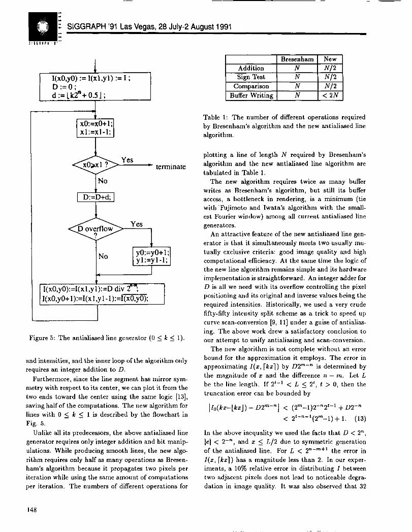
Figure 5: The antialiased line generator (O s k < 1).
and intensities, and the inner loop of the algorithm only
requires an integer addition to D.
Furthermore, since the line segment has mirror sym-
metry with respect to its center, we can plot it from the
two ends toward the center using the same logic [13],
saving half of the computations. The new algorithm for
lines with O ~ k ~ 1 is described by the flowchart in
Fig. 5.
Unlike all its predecessors, the above antialiased line
generator requires only integer addition and bit manip-
ulations. While producing smooth lines, the new algo-
rithm requires only half ss many operations as Bresen-
ham’s algorithm because it propagates two pixels per
iteration while using the same amount of computations
per iteration. The numbers of different operations for
Comparison N N;2
Buffer Writing N < 2N
Table 1: The number of different operations required
by Bresenham’s algorithm and the new antialiased line
algorithm.
plotting a line of length N required by Bresenham’s
algorithm and the new antialiased line algorithm are
tabulated in Table 1.
The new algorithm requires twice as many buffer
writes as Bresenham’s algorithm, but still its buffer
access, a bottleneck in rendering, is a minimum (tie
with -Fujimoto and Iwata’s algorithm with the small-
est Fourier window) among all current antialiased line
generators.
An attractive feature of the new antialiased line gen-
erator is that it simultaneously meets two usually mu-
tually exclusive criteria: good image quality and high
computational efficiency. At the same time the logic of
the new line algorithm remains simple and its hardware
implementation is straightforward. An integer adder for
D is all we need with its overflow controlling the pixel
positioning and its original and inverse values being the
required intensities. Historically, we used a very crude
fifty-fifty intensity split scheme as a trick to speed up
curve scan-conversion [9, 11] under a guise of antialias-
ing. The above work drew a satisfactory conclusion to
our attempt to unify antialiasing and scan-conversion.
The new algorithm is not complete without an error
bound for the approximation it employs. The error in
approximating 1(z, [kz] ) by D2m-” is determined by
the magnitude of z and the difference n – m. Let L
be the line length. If 2~-1 < L s 2*, f >0, then the
truncation error can be bounded by
IZo(kz-[kzj) - D2m-” I < (2m-1)2-”2’-’ + D2-n
< Z’-n-’(zl)+)+ 1. (13)
In the above inequality we used the facts that D < 2“,
Iel < 2-n, and x < L/2 due to symmetric generation
of the antialiased line. For L < 2n–m+l the error in
I(z, [kzl ) has a magnitude less than 2. In our exper-
iments, a 10~0 relative error in distributing 1 between
two adjacent pixels does not lead to noticeable degra-
dation in image quality. It was also observed that 32
148

@ @ Computer Graphics, Volume 25, Number 4, July 1991
different gray scales are sufficient to eliminate the most
of aliasing, For a 1024 x 1024 display, the maximum
L <211 (t = 11). Suppose that 32 gray scales (m = 5)
is used for antialiasing. Then we need n ~ 15 to bound
the error in I(r, [kzl ) by 2, or the relative error by
0,063. This only requires D to be a twobytes integer.
Our recent research revealed that the proposed an-
tialiased line algorithm is particularly suitable to be in-
corporated into a logic-enhanced frame buffer to solve
the bottleneck of frame buffer access [14]. An intelligent
frame buffer architecture in the form of wavefront ar-
ray processors was designed to scan-convert lines right
inside the frame buffer. This design achieves extremely
high rendering throughput with very low frame buffer
bandwidth requirement.
6 Fast Anti-Aliased Circle
Generator
Due to the 8-way symmetry of the circle, it sutfices to
consider the circle X2 + yz ,= r2 in the first octant. For
the circle equation, the two-point antialiasing scheme
Eq(3) becomes
Now we derive the
(14)
algorithm to compute Eq(14) as j
marches in the y axis from O to > in scan-converting
the first octant circular arc. The first issue is to de-
1termine when the integer-valued function ~-
1decreases by 1 as j increases. We need the critical val-
1~ 2ues t such that r - (t – 1)2] – [/-] = 1 to
move the pixel band being plotted to the left by one
step. This computation can be simplified by the follow-
ing lemma.
LEMMA 1
~~e relation [/r’ -(~- 1)21 -[m= 1 holds
if and only if [/r’ -(t- 1)2] - ~r2-(t - 1)’ >
[/-] - J-.
Proof. Since ~~ is monotonically decreasing in
~? [@-(~- 1)’] -/ r’ – (t – 1)2 > [~~1 –
= implies [/r’- (~- 1)’1 -I=> o
But in the first octant we have
r2–(’–l)2– <-<l (15)
prohibiting [i.’ -(f- 1)21 - [~~1 > I hence
1~ 1r’ –(t – 1)2 – (<=1 = 1.
The only-if part can be proven by contradiction.
Assume that ({r,-(t - 1)~1 - ~~~~ = I but
[/r’ -(f - 1)’] - <r’ -(~- 1)2 s [J-1 -
~. This requires ~ r2–(t–1)2–~~>1,
an impossibility in the first octant. •l
[ 1--!1<For given r the values ~-
~<~, serve dual purposes: determining the pixel po-
sitions as suggested by the above lemma and determin-
ing the pixel intensities as in Eq( 14). Let the intensity
range for the display be from O to 2m – 1 and define the
integer variable
D(r, j) = I(2M – 1) ([/m] - J-) +0.5J
(16)
Then it follows from Eq( 14) that
1 (~~~1 ,j) = D(r,j)
(1 1)I-)j = D(r, j), l<j< ;,(17)
where D(r, j) is the integer value obtained through
bitwise-inverse operation on D(r, j) since
~([=l,.i)+~([~]jj)= 1=2”–1
(18)
and since the intensity values are integers. By Eq(16)
[ 1every decrement of the function <~ – ~-
as j increases is reflected by a decrement of D(r, j), thus
D(r, j) can be used to control the scan-conversion of
the circle. The new antialiased circle algorithm based
on precomputed D(r, j) is extremely simple and fast.
The algorithm for the first octant is described by the
flowchart in Fig. 6.
The inner loop of the antialiased circle algorithm re-
quires even fewer operations than Bresenham’s circle
algorithm. Of course, the gains in image quality and
scan-conversion speed are obtained by using the D(r, j)
table. If R~~x is the maximum radius handled by the
circle generator, then the table size will be ~Rma=. It
is my opinion that the rapidly decreasing memory cost
makes the above simple idea a viable solution to real-
time antialiased circle generation. For instance, for a
64K bytes ROM the above algorithm can display an-
tialiased circular arcs of radius up to 430, \Vithout the
I 49

EE.: SIGGRAPH ’91 Las Vegas, 28 July-2 August 1991
$ICG!APH11-
Ci:=r;
j:=qI(i,j):=I;T:= O;
Yes- terminate
Yes
1No i := i-1;
- I
tI(i,j):=~,I(i-1 ,j):=D(r,j);T:=D(r,j);
I
Figure 6: Antialiased circle generator (lst octant).
precomputed table D(r, j) the antialissed circle alg~
rithm can be implemented by computing the function
D(r, j).
The performance of the new antialiased circle alg~
rithm is demonstrated by Fig. 7.
7 Other Antialiasing Issues
We demonstrated that the new antialiasing technique
is particularly efficient for generating antialiased lines
and circles since Eq(3) can be incorporated into the
classical incremental curve scan-conversion framework.
But it is not restricted to those two graphics primi-
tives. The intensity interpolation of Eq(3) applies to
any curves or object edges. We should not partition a
general curve into line segments and then antialias line
Figure 7: Circles by Bresenham’s (above) and the new
antialiasing algorithms (below).
150

630 Comwter GraDhics. Volume 25. Number 4. Julv 1991
segments as suggested by some authors before. Insteadan antialiased curve can be computed by directly scan-converting the curve, i.e., for increasing raster ordinatei, computing f(i) and then interpolate the intendedcurve intensity Is between the two pixels (i, Lr(i)J) and(i, [f(i)]). The main cost is to compute the real valuef(i), but it is required by scan-conversion anyway. Soantialiasing will not be a computational burden for gen-eral curves.
Although our algorithms were presented for antialias-ing curves, their extension to object boundaries isstraightforward. We simply partition the object bound-aries into x-dominant and y-dominant curve segments,and scan-convert them. It is easy to determine whichside of such a curve segment is exterior. We use Eq(3)to interpolate the object color on two adjacent pixelsat the two sides of the continuous boundary curve, andthen blend the outer pixel value with the backgroundcolor. Let Ic and Ib be the intensities (colors) for objectand its background, and d < 1 be the distance betweenthe outer pixel and the true object boundary, then theblending formuIa for the boundary pixel is
I = dlo + (1 - d)lb. (19)
Note that unlike the blending formula by Fujimoto andIwata [6] no division is required here. Furthermore, forantialiasing polygon edges in uniform background, wecan solve Eq(19) incrementally with only integer addi-tions and binary shifts much like our antialiased linealgorithm. We will not pursue this efficiency issue anyfurther due to the space limitation. The performance ofthe new technique on antialiased object edges in color-ful background is shown by Fig. 8, where a filled circlewit11 antialiasing in a complex background is comparedwith the one without. The antialiased filled circle ap-pears smooth and sharp. Note that the results of Fig.8 were obtained on an g-bit color device, so color quan-tization was necessarily performed. On a 24-bit colordevice with more subtle shades available the antialiaseddisk looked even better.
Our antialiasing technique has the same subpixel ad-dressability as Fujimoto-Iwata’s method due to theirequivalence.
8 Conclusion
Unlike all previous antialiasing research, our two-pointantialiasing scheme was derived in spatial domain un-der a subjectively meaningful error measure to preserve
Figure 8: Filled circles embedded in colorful back-ground without antialiasing (above) and with antialias-ing (below).
151

SIGGRAPH ’91 Las Vegas, 28 July-2 August 1991
dynamic information of the original curves or object
edges. The behaviour of this antialiasing scheme in fre-
quency domain was also analyzed. It was shown that
the new antialiasing technique can generate smooth line
segments and circular arcs at even higher speeds than
those of Bresenham’s line and circle algorithms. The
hardware or assembly-language realization of our new
antialiasing algorithms ia straightforward. These fea-
tures have practical significance when antialiasing is
performed on small economical graphics devices or in
time-constrained applications.
Acknowledgment
The author gratefully acknowledges the financial sup-
port of the Canadian Government through NSERC
grant 0GPO041926 and thanks SIGGRAPH reviewers
for their polishing of his original manuscript.
References
[1]
[2]
[3]
[4]
[5]
[6]
[7]
[8]
A. C. Barkans, “High speed high quality an-
tialiased vector generation,” Computer Graphics,
vol. 24, no. 4, p. 319-326, Aug. 1990.
J. E. Bresenham, “Algorithm for computer control
of digital plotter,” IBM Syst. J., vol. 4, no. 1, 1965,
p. 25-30.
J. E. Bresenham, “A linear algorithm for incremen-
tal digital display of circular arcs”, Comm. ACM,
vol. 20, no. 2, 1977, p. 750-752.
F. Crow, “The aliasing problem in computer-
generated shaded images: Comm. ACM, vol. 20,
no. 11, Nov. 1977.
D. Field, “Algorithms for drawing anti-aliased cir-
cles and ellipses,” Computer Vision, Graphics, and
Image l%oc., vol. 33, p. 1-15, 1986.
A. Fujimoto and K. Iwata, “Jay-free images on
raster displays,” IEEE CG&A, vol. 3, no. 9, p. 26-
34, Dec. 1983.
S. Gupta and R. F. Sproull, “Filtering edges for
gray-scale displays,” Computer Graphics, vol. 15,
no. 3, p. 1-5, Aug. 1981.
M. Pitteway and D. Watkinson, “Bresenham’s al-
[9]
10]
11]
[12]
[13]
[14]
X. Wu and J. Rokne, “Double-step incremental
generation of lines and circles”, Computer Vision,
Graphics, Image Proc., vol. 37, 1987, p. 331-344.
X. Wu and J. Rokne, “On properties of discretized
convex curves,” IEEE Thans. Pattern Analysis and
Machine Intelligence, vol. 11, p. 217-223, Feb.
1989.
X. Wu and J. Rokne, “Double-step generation of
ellipses”, IEEE CG&A, vol. 9, no. 3. p. 56-69, May
1989.
X. Wu and J. Rokne, “Dynamic error mea-
sure for curve scan-conversion,” Proc. Graph-
ics/interface ’89, London, Ontario, p. 183-190,
June 1989.
J. Rokne, B. Wyvill and X. Wu, “Fast line scan-
conversion ~ ACM Trans. on Graphics, vol. 9, no.
4, p. 377-388, oct. 1990,
X. Wu, “A frame buffer architecture for parallel
vector generation,” Proc. Graphics/Interface ’91,
Calgary, June 1991.
gorithm with gray scale: Comm. ACM, vol 23, no.
11, November 1980.
152