an efficient algorithm for constructing optimal design of computer
TRANSCRIPT
1
An Efficient Algorithm for Constructing Optimal Design of Computer Experiments
Ruichen Jin, Wei Chen1 Integrated DEsign Automation Laboratory (IDEAL)
Northwestern University
Agus Sudjianto V-Engine Engineering Analytical Powertrain
Ford Motor Company
Publishing Corresponding Author Dr. Agus Sudjianto
V-Engine Engineering Analytical Powertrain 21500 Oakwood Blvd., Dearborn, MI 48121-4091
POEE Bld., EC 118, MD 68 Phone: (313) 390-7855, E-mail: [email protected]
Abstract The long computational time required in constructing optimal designs for computer
experiments has limited their uses in practice. In this paper, a new algorithm for
constructing optimal experimental designs is developed. There are two major
developments involved in this work. One is on developing an efficient global optimal
search algorithm, named as enhanced stochastic evolutionary (ESE) algorithm. The other
is on developing efficient methods for evaluating optimality criteria. The proposed
algorithm is compared to existing techniques and found to be much more efficient in
terms of the computation time, the number of exchanges needed for generating new
designs, and the achieved optimality criteria. The algorithm is also very flexible to
construct various classes of optimal designs to retain certain desired structural properties.
Key words: optimal design, computer experiments, stochastic evolutionary algorithm
1 Technical corresponding author: Dr. Wei Chen, Department of Mechanical Engineering, Northwestern University, Evanston,
IL 60208-3111, [email protected].

2
1. INTRODUCTION
Building surrogate models (or called metamodels) based on computer experiments
has been widely used in engineering design due to the high computational cost of using
high-fidelity simulations. Design of computer experiments, or called sampling (for
simulations) has a considerable effect on the accuracy of a metamodel. To improve the
space-filling property as well as to maintain a good computational efficiency in sampling,
some researchers proposed to search an optimal design within a class of designs that have
desirable structural properties, e.g., the Latin hypercube designs (LHD) (McKay, et al.,
1979) with good one-dimensional projective property. Morris and Mitchell (1995)
introduced optimal LHDs based on the pφ criterion (a variant of the maximin distance
criterion, see Johnson, et. al., 1990); Park (1994) introduced optimal LHDs based on
either the maximum entropy criterion or the integrated mean squared-error (IMSE)
criterion; Fang, et al (2002) introduced optimal LHDs based on the Centered L2
discrepancy criterion.
Searching the optimal design of experiments within a class of designs, even though
more tractable than searching in the entire sample space without any restrictions, is still
difficult to solve exactly. An exhaustive search method is computationally prohibitive
even for a small problem. For example, for optimizing 10×4 LHDs (10 runs, 4 factors),
the number of distinct designs is more than 1022. It is more practical to solve optimal
design (of experiments) problems approximately. Toward this effort, Morris and
Mitchell (1995) adapted a version of simulated annealing (SA) algorithm for constructing
optimal LHDs; Park (1994) developed a rowwise element exchange algorithm for
constructing optimal LHDs; Ye, et al (2000) used the columnwise-pairwise (CP)
algorithm (Li and Wu, 1997) for constructing optimal symmetrical LHDs; Fang, et al
(2002) adapted the threshold accepting (TA) algorithm (essentially a variant of SA) in
constructing optimal LHD. The optimal designs constructed by these algorithms have
been shown to have a good space-filling property. However, the computational cost of
these existing algorithms is generally high. For example, Ye, et al (2000) reported that
generating an optimal 25×4 LHDs using CP could take several hours on a Sun SPARC 20
workstation. For a design as large as 100×10, the computational cost could be
formidable; thus, search processes often stop before finding a good design.
3
In this paper, we propose an algorithm that is not only able to quickly construct a
good design of experiments given a limited computational resource but also capable of
moving away from a locally optimal design. The proposed method is especially useful
for constructing median to large-sized design of experiments. For example, for a 100×10
LHD, the proposed algorithm is able to find a good design within minutes, if not within
seconds. Furthermore, the algorithm is able to work on different classes of designs and
maintain desirable special structural properties, e.g., the balance property of LHDs and
the orthogonality of OA (Owen, 1992; Hedayat et al., 1999) and OA-based LHDs (Tang,
1993). In this paper, we only show how it is used to optimize LHDs. The extensions to
optimizing other classes of designs can be found in Jin 2003.
2. THE TECHNOLOGICAL BASE
An experimental design with n runs and m factors is usually written as an n×m matrix
X = [x1, x2,...,xn]T, where each row xiT
=[xi1, xi2,..., xim] stands for an experimental run and
each column stands for a factor or a variable. The optimal experimental design problem
we are interested is to search a design X* in a given design class Z, which optimizes (for
simplicity, minimization is considered) a given optimality criterion f, i.e,
)(min XX
fZ∈
. (1)
2.1. Optimality Criteria
Optimal criteria are used to achieve the space-filling property in design of computer
experiments. Three widely used optimality criteria are considered in this work.
Maximin Distance Criterion and φp Criterion
A design is called a maximin distance design (Johnson, et al, 1990) if it maximizes
the minimum inter-site distance:
),(min,,1
jijinjid xx
≠≤≤, (2)
where d(xi, xj) is the distance between two sample points xi and xj:
21,),(/1
1ortxxdd
tm
k
tjkikijji =
⎥⎥⎦
⎤
⎢⎢⎣
⎡−== ∑
=xx . (3)
4
Morris and Mitchell (1995) proposed an intuitively appealing extension of the
maximin distance criterion. For a given design, by sorting all the inter-sited distance dij
(1≤ i, j ≤n, i ≠ j ), a distance list (d1, d2, ..., ds) and an index list (J1, J2,..., Js) can be
obtained, where di’s are distinct distance values with d1<d2<...<ds, Ji is the number of
pairs of sites in the design separated by di, s is the number of distinct distance values. A
design is called a φp-optimal design if it minimizes: ps
i
piip dJ
/1
1 ⎥⎥⎦
⎤
⎢⎢⎣
⎡= ∑
=
−φ , (4)
where p is a positive integer. With a very large p, the φp criterion is equivalent to the
maximin distance criterion.
Entropy Criterion
Shannon (1948) used entropy to quantify the "amount of information": the lower the
entropy, the more precise the knowledge is. Minimizing the posterior entropy is
equivalent to finding a set of design points on which we have the least knowledge. It has
been further shown that the entropy criterion is equivalent to minimizing the following
(see, e.g., Koehler and Owen, 1996):
Rlog− , (5)
where R is the correlation matrix of the experimental design matrix Tn ],...,,[ 21 xxxX = ,
whose elements are:
21;,1,exp1
≤≤≤≤⎟⎟⎠
⎞⎜⎜⎝
⎛−−= ∑
=tnjixxR
m
k
tjkikkij θ , (6)
where θk (k=1,..,m) are correlation coefficients.
Centered L2 Discrepancy Criterion
The Lp discrepancy is a measure of the difference between the empirical cumulative
distribution function of an experimental design and the uniform cumulative distribution
function. In other words, the Lp discrepancy is a measure of non-uniformity of a design.
Among Lp discrepancy, L2 discrepancy is used most frequently since it can be expressed
analytically and is much easier to compute. Hickernell (1998) proposed three formulas of

5
L2 discrepancy, among which the centered L2-discrepancy (CL2) seems the most
interesting.
.)215.0
215.0
211(1
)5.0215.0
211(2
1213)(
1 1 12
1 1
22
22
∑∑∏
∑∏
= = =
= =
−−−+−++
−−−+−⎟⎠⎞
⎜⎝⎛=
n
i
n
j
m
kjkikjkik
n
i
m
kikik
xxxxn
xxn
CL X (7)
A design is called uniform design if it minimizes the centered L2 discrepancy (Fang,
et al, 2000).
2.2. Updating Operations and Search Algorithms
A typical experiment-constructing algorithm is repeated in the following procedure:
1. Start from a randomly chosen starting design X0;
2. Construct a new design (or a set of new designs) by some kinds of updating
operations on the current design;
3. Compute the criterion value of the new design and decide whether to replace the
current design with the new one.
There are two major types of updating operations, i.e., rowwise operations and
columnwise operations (Li and Wu, 1997). We are interested in columnwise operations
since they are particularly easier to keep the structure properties of a design in relation to
columns, such as the balance and orthogonality properties. In this study, we focus on a
particular type of columnwise operation, called element-exchange, which interchanges
two distinct elements in a column and guarantee to retain the balance property. Take a
5×4 LHD for example:
1 2 4 0 3 4 0 3 2 1 3 4 4 0 1 2 0 3 2 1
Exchange two elements in the second column
1 2 4 0 3 0 0 3 2 1 3 4 4 4 1 2 0 3 2 1
Figure 1. Element-exchange in a 5×4 LHD
6
Obviously, after the element-exchange, the balance property of 2nd column is
retained, while the design is still a LHD. Another advantage of using element-exchange,
as to be shown in Section 3.2, is that the evaluation of an optimal criterion of a new
design induced by an element-exchange can be very efficient.
The three existing optimization search algorithms for optimal DOEs are reviewed
here with the highlights of their differences. The CP algorithm (Li and Wu, 1997) starts
from an n×m randomly chosen design X. Each iteration in the algorithm is divided into m
steps. At the ith step, the CP algorithm compares all possible distinct designs and selects
the best design Xtry from all those designs. If after an iteration, Xtry is better than X, i.e.,
f(Xtry) < f(X), the procedure will be repeated; if no improvement is achieved at an
iteration, the search will be terminated. The CP algorithm could quickly find a locally
optimal design. However, depending on the starting design, the optimal design obtained
could be of low quality. In practice, with the CP algorithm, the optimization process
needs to repeat for Ns cycles from different starting designs and the best design is
selected. Because CP algorithm compares all possible exchange within a column to
select the best element exchange, the computational requirement can be excessively large
when n is large. Li and Nachtsheim (2000) proposed the restricted CP algorithm as an
improvement of the original CP algorithm. In that algorithm, only a fraction of all pair
exchanges in a column is considered. The approach can be applied to reduce the number
of element exchange candidates for general factorial designs but not space filling design
such as LHD.
With the SA algorithm (Morris and Mitchell, 1995), a new design Xtry replaces X if it
leads to an improvement. Otherwise, it will replace X with probability of
})]()([exp{ Tff try XX −− , where T is a parameter called “temperature” in the
analogous physical process of annealing of solids. Initial set to T0, T will be
monotonically reduced by a cooling schedule. Morris and Mitchell used T’ = αT as the
cooling schedule, where α is a constant called cooling factor here. SA usually converges
slowly to a high quality design. The TA algorithm (Winker and Fang, 1998) is
essentially a variant of the SA, with a simple deterministic acceptance criterion:
7
htry Tff ≤− )()( XX , where Th is called “threshold”. Th is monotonically reduced based
on a cooling schedule. TA has been used for constructing uniform designs (c.f., Fang
2000; Fang, et al, 2002).
3. PROPOSED ALGORITHM FOR CONSTRUCTING OPTIMAL
EXPERIMENTAL DESIGN
To overcome the difficulties associated with the existing methods and to achieve
much improved efficiency, our proposed method adapts and enhances a global search
algorithm, i.e., the stochastic evolutionary algorithm (Section 3.1), and utilizes efficient
methods for evaluating different optimality criteria (Section 3.2) to significantly reduce
the computational burden.
3.1. Enhanced Stochastic Evolutionary (ESE) Algorithm
The enhanced stochastic evolutionary (ESE) algorithm is adapted and enhanced from
the stochastic evolutionary (SE) algorithm, which was originally developed by Saab and
Rao (1991) for general combinatorial optimization applications. With SE, whether to
accept a new design is decided by a threshold-based acceptance criterion, but its strategy
(or schedule) to change the value of threshold is different from that of TA or SA. It is
shown (Saab and Rao, 1991) that SE can converge much faster than SA. SE is also
capable of moving away from low quality local optimum to find a high quality solution.
However, adjusting the initial threshold Th0 and the warming schedule for different
problems is still quite troublesome with the original SE. The ESE algorithm developed in
this work uses a sophisticated combination of warming schedule and cooling schedule to
control Th so that the algorithm can be self-adjusted to suit different experimental design
problems (i.e., different classes of designs, different optimality criteria, and different
sizes of designs).
8
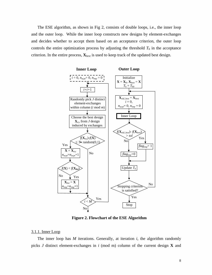
The ESE algorithm, as shown in Fig 2, consists of double loops, i.e., the inner loop
and the outer loop. While the inner loop constructs new designs by element-exchanges
and decides whether to accept them based on an acceptance criterion, the outer loop
controls the entire optimization process by adjusting the threshold Th in the acceptance
criterion. In the entire process, Xbest is used to keep track of the updated best design.
Inner Loop Outer Loop
Randomly pick J distinct element-exchanges
within column (i mod m)
Choose the best design Xtry from J design
induced by exchanges
X = Xtry nacpt=nacpt+1
i < M
No
Yes
i = 0, nacpt= 0, nimp = 0
Yes
f(X) < f(Xbst)
Xbst = X nimp=nimp+1
No
Yes
i=i+1
Xold_best = Xbest i = 0,
nacpt= 0, nimp = 0
Inner Loop
f(Xold_best)- f(Xbest) > tol
flagimp= 1
Stopping criterion is satisfied?
flagimp=0
No
Update Th
Yes
Initialize X = X0, Xbest = X
Th = Th0
No
Stop
Yes
f(Xtry)-f(X) ≤ T• random(0,1)
No
Figure 2. Flowchart of the ESE Algorithm
3.1.1. Inner Loop
The inner loop has M iterations. Generally, at iteration i, the algorithm randomly
picks J distinct element-exchanges in i (mod m) column of the current design X and

9
chooses the best design Xtry based on the values of optimal criterion. If Xtry is better than
the current design X, it will be accepted to replace X; otherwise, Xtry will be accepted to
replace X if it satisfies the following acceptance criterion:
)1,0(random⋅≤∆ hTf , (8)
where )()( XX fff try −=∆ , random(0,1) is a function that generates uniform random
numbers between 0 and 1 and Th > 0 is a control parameter, which is called threshold
here. If hTf ≥∆ , Xtry will never be accepted and if hTf <∆<0 , let S = random(0,1), then
Xtry will be accepted with probability:
hh TfTfSP ∆−=∆≥ 1)( . (9)
With this acceptance criterion, a temporarily worse design could be accepted and a
slightly worse design (i.e., a small f∆ ) is more likely to replace the current design than a
significantly worse design (i.e., a large f∆ ). In addition, a given increase in criterion
value is more likely to be accepted if Th has a relatively high value. The setting of Th will
be discussed later.
The values of parameters involved in the inner loop, i.e., J and M, are pre-
specified. Unlike CP, which compares all possible distinct designs induced by
exchanges, our algorithm only randomly picks J distinct designs resulted from
exchanges. Based on our testing experience, too large of J may make it more possible to
be stuck in a locally optimal design for small-sized designs and lead to low efficiency for
large-sized designs. Based on our tests, we set J to be ne/5 but no large than 50, where ne
is the number of all possible distinct element-exchanges in a column ( ⎟⎟⎠
⎞⎜⎜⎝
⎛2n
for a LHD and
2)/(2 ii qn
q×⎟⎟⎠
⎞⎜⎜⎝
⎛ for a balanced design). For mixed-level balanced designs, the values of J
will be different for different columns. The parameter M is the number of iterations in
the inner loop, i.e., the number of tries the algorithm will make before going on to the
next threshold Th. It seems reasonable that M should be larger for larger problems. In our
test, we set M to be Jmne /2 but no larger than 100.
10
3.1.2. Outer Loop
The outer loop controls the optimization process by updating the value of the
threshold Th. At the beginning of the optimization process, Th is set to be a small value,
i.e., Th0 = 0.005×criterion value of the initial design. Later on it will be adjusted and
maintained based on whether the search is within the so-called improving process or
exploration process. A search process is turned to the improving process (flagimp = 1) if
the criterion is improved after a cycle (an inner loop). Once turning to the improving
process, Th is adjusted to rapidly find a locally optimal design. If no improvement is
made after a cycle, the search process will be turned to the exploration process (flagimp =
0), during which Th is adjusted to help the algorithm escape from a locally optimal
design. The maximum number of cycles is used as the stopping criterion.
Based on our tests, the following proposed schedules for controlling Th is found to
work very well for different experimental design problems:
1. In the improving process, Th is maintained on a small value so that only better
design or slightly worse design will be accepted. Unlike the original SE, the value of Th
will not be fixed to Th0. Instead, Th will be updated based on the acceptance ratio nacpt/M
(number of accepted design versus the number of tries in the inner loop) and the
improvement ratio nimp/M (number of improved design versus the number of tries in the
inner loop). Specifically, Th will be decreased if the acceptance ratio is larger than a small
percentage (e.g., 10%) and the improvement ratio is less than the acceptance ratio; Th will
be maintained in the current value if the acceptance ratio is larger than the small
percentage and the improvement ratio is equal to the acceptance ratio (meaning that Th is
so small that only improving designs are accepted by the acceptance criterion); Th will be
increased otherwise. The following equations are used in our algorithm to decrease and
increase Th, respectively, TT 1' α= and 1/' αTT = , where 10 1 <<α . The setting of 1α =
0.8 appears to work well in all tests.
2. In the exploration process, Th will fluctuate within a range based on the acceptance
ratio. If the acceptance ratio is less than a small percentage (e.g., 10%), Th will be rapidly
increased until the acceptance ratio is larger than a large percentage (e.g. 80%). If this
happens, Th will be slowly decreased until the acceptance ratio is less than the small
percentage. This process will be repeated until an improved design is found. The
following equations are used to decrease and increase Th, respectively, TT 2' α= and
11
3/' αTT = , where 10 23 <<< αα . Based on our experience, we set 2α = 0.9 and 3α =
0.7. Th is increased rapidly (so that more worse designs could be accepted) to help
moving away from a locally optimal design. Th is decreased slowly for searching better
designs after moving away from the local optimal design.
3.2. Efficient Methods for Evaluating Optimality Criteria
As an optimality criterion is repeatedly evaluated whenever a new design of
experiments is constructed, the efficiency of this evaluation becomes critical for
optimizing the design of experiment within a reasonable time frame. In this work, we
propose efficient evaluation methods that take into account the feature of our updating
operation, i.e., when using columnwise element-exchanges for generating new designs,
only two elements in the design matrix are involved each time. The evaluations of
optimal criteria, such as pφ criterion, the entropy criterion, and the CL2 criterion, involve
different types of matrices (e.g., the inter-distance matrix D, the correlation matrix R, and
the discrepancy matrix C, respectively). Re-evaluating all the elements in the matrices
each time is not affordable, especially if the matrix size is large (determined by the
number of experiments and number of factors).
φp Criterion The re-evaluation of φp based on Eq. 4 includes three parts, i.e., the evaluation of all
the inter-site distances, the sorting of those inter-site distances to obtain a distance list
and index list, and the evaluation of φp. The evaluation of all the inter-site distances will
take O(mn2), the sorting will take O(n2log2(n)) (c.f. Press, et al, 1997), and the evaluation
of φp will take O(s2log2(p)) (since p is an integer, p-powers can be computed by repeated
multiplications). In total, the computational complexity will be
O(mn2)+O(n2log2(n))+O(s2log2(p)). Therefore, re-evaluating φp will be very time-
consuming.
Before introducing the new method, a new equation of φp is first provided, which
helps develop an efficient evaluation algorithm by avoiding the sorting required by Eq. 4.
Let nnijd ×= ][D be a symmetric matrix, whose elements are the inter-site distances of the
current design X, the new equation, called p-norm form here, is expressed by:

12
( )p
nji
pij
p
nji
pijp dd
/1
1
/1
1/1
⎥⎥⎦
⎤
⎢⎢⎣
⎡=
⎥⎥⎦
⎤
⎢⎢⎣
⎡= ∑∑
≤<≤
−
≤<≤φ . (10)
The equivalence between this form and Eq. 4 can be easily proved, which is omitted here.
Our new algorithm takes into account the fact that after an exchange ( kiki xx 21 ↔ ),
only elements in rows i1 and i2 and columns i1 and i2 are changed in D matrix. For any
21,and1 iijnj ≠≤≤ , let:
t
jkkit
jkki xxxxjkiis −−−= 1221 ),,,( , (11)
then:
[ ] ttjijiji jkiisddd
/121111 ),,,('' +== (12)
and
[ ] ttjijiji jkiisddd
/121222 ),,,('' −== . (13)
With the above representation, the computational complexity of updating the
elements in D matrix is O(n). The new pφ is now computed by:
[ ] [ ]p
iijnj iijnj
pji
pji
pji
pji
ppp dddd
/1
2,1,1 2,1,12211
' )'()'(⎥⎥⎦
⎤
⎢⎢⎣
⎡−+−+= ∑ ∑
≠≤≤ ≠≤≤
−−−−φφ , (14)
of which the computational complexity is O(n log2(p)). The total computational
complexity of the new algorithm is O(n)+O(n log2(p)). This results in significant
reduction of computation compared to re-evaluating φp.
Entropy Criterion
Since the correlation matrix nnijr ×= ][R in Eq. 6 is positive-definite, it can be expressed
by Cholesky decomposition:
UUR *T= , (15)
where, nniju ×= ][U is an upper triangle matrix, i.e., jiuij <= if0 .
Therefore,
∏=
=n
iiiu
1
2R . (16)
13
The computational complexity of Cholesky factorization (or decomposition) is O(n3). In
addition, the calculation of the elements of R costs O(mn2), and therefore the
computational complexity for totally re-evaluating the entropy will be O(mn2)+O(n3) .
While the determinant of the new R matrix cannot be directly evaluated based on the
determinant of the old R matrix, by modifying the Cholesky algorithm, some
improvement in efficiency is achievable. Let n1=min(i1,i2), then R can be written as:
⎥⎦
⎤⎢⎣
⎡=
−×−−×
−×××
)()(3)(2
)(21
1111
1111
)()()()(
nnnnnnnT
nnnnnnn RR
RRR . (17)
If the Cholesky factorization of R1 is known, i.e., 111 '*UUR = , the Cholesky
factorization U of R can be computed based on U1:
⎥⎦
⎤⎢⎣
⎡=
−×−
−××
)()(3
)(21
11
1111
)(0)()(
nnnn
nnnnn
UUU
U (18)
where U3 is also an upper triangle matrix. Therefore, the elements of U with index
11 nji ≤≤≤ are kept unchanged. The rest of the elements in the upper triangle matrix U
can be calculated by following a modified Cholesky factorization algorithm (see Jin,
2003 for details).
The computational complexity of the modified Cholesky factorization algorithm will
depend on both n and n1. For example, if n1=n-1, the computational complexity will be
O(n2). On the other hand, if n1=1, the computational complexity will be still O(n3). In
average, the computational complexity will be smaller than O(n3) but larger than O(n2).
The total computational complexity of the new mthod will be between O(n) + O(n2) and
O(n) + O(n3), which is not dramatically better than O(n3)+O(mn2).
CL2 Criterion
Evaluating the CL2 criterion employs a similar idea as that for the pφ criterion. Let
mnikz ×= ][Z be the centered design matrix of X, i.e., 5.0−= ikik xz . Let nnijc ×= ][C be a
symmetric matrix, whose elements are:
14
⎪⎪⎩
⎪⎪⎨
⎧
−+−+
≠−−++=
∏∏
∏
==
=
otherwisezzn
zn
jiifzzzznc m
kikik
m
kik
m
kjkikjkik
ij
1
2
12
12
)21||
211(2|)|1(1
)||||2(211
(19)
Let ∏=
+=m
kiki zg
1
|)|1( and ∏∏==
−+=−+=m
kikik
m
kikiki zzzzh
11
2 |)|2|)(|1(21)
21||
211( , then,
nhngc iiii /2/ 2 −= . (20)
It can be easily proved that: ∑∑= =
+⎟⎠⎞
⎜⎝⎛=
n
i
n
jijcCL
1 1
22
2 1213)(X (21)
The computational complexity of totally re-evaluating CL2 discrepancy is O(mn2).
After an exchange kiki xx21
↔ , only elements in i1 and i2 rows and i1 and i2 columns of C
are changed. For any 21,and1 iijnj ≠≤≤ , let
)||||2()||||2(),,,(112221 jkkijkkijkkijkki zzzzzzzzjkii −−++−−++=γ , (22)
then,
jijiji cjkiicc111
),,,('' 21γ== (23)
and
),,,(/'' 21222jkiiccc jijiji γ== . (24)
Let |)|1(|)|1(),,(1221 kiki zzkii ++=α and |)|2(|)|2(),,(
1221 kiki zzkii −−=β , then:
nhkiikiingkiic iiii /),,(),,(2/),,('1111 2121
221 βαα −= , (25)
and
)],,(),,(/[2)],,(/[' 2121212
2222kiikiinhkiingc iiii βαα −= . (26)
The computational complexity of updating the C matrix is O(n).
The new CL2 can be computed by:
∑≠≤≤
−+−×+−+−+=n
iijnjjijijijiiiiiiiii ccccccccCLCL
21
221122221111,,1
22
22 )''(2'')'( , (27)
whose computational complexity is O(n). The total computational complexity is also
O(n), which is much less than O(mn2).
A comparison of the computational complexity of totally re-evaluating all
elements in matrices and those of our new methods are summarized in Table 1. From the
15
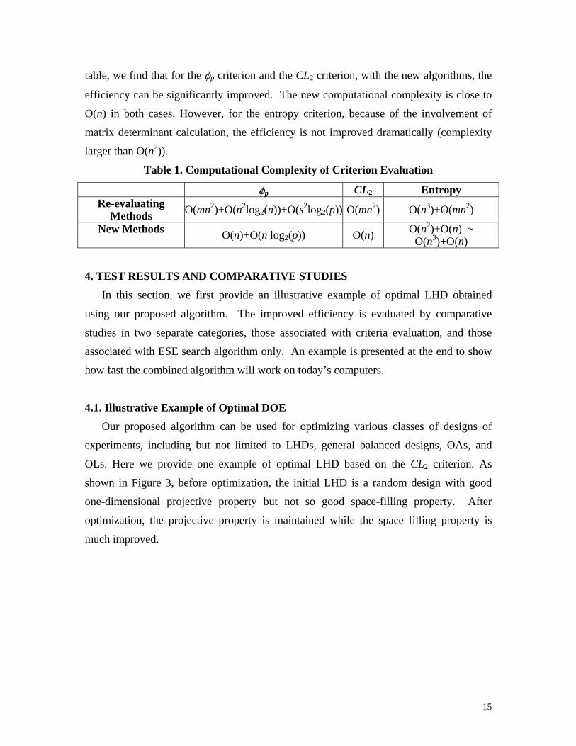
table, we find that for the φp criterion and the CL2 criterion, with the new algorithms, the
efficiency can be significantly improved. The new computational complexity is close to
O(n) in both cases. However, for the entropy criterion, because of the involvement of
matrix determinant calculation, the efficiency is not improved dramatically (complexity
larger than O(n2)).
Table 1. Computational Complexity of Criterion Evaluation
φp CL2 Entropy Re-evaluating
Methods O(mn2)+O(n2log2(n))+O(s2log2(p)) O(mn2) O(n3)+O(mn2)
New Methods O(n)+O(n log2(p)) O(n) O(n2)+O(n) ~ O(n3)+O(n)
4. TEST RESULTS AND COMPARATIVE STUDIES
In this section, we first provide an illustrative example of optimal LHD obtained
using our proposed algorithm. The improved efficiency is evaluated by comparative
studies in two separate categories, those associated with criteria evaluation, and those
associated with ESE search algorithm only. An example is presented at the end to show
how fast the combined algorithm will work on today’s computers.
4.1. Illustrative Example of Optimal DOE
Our proposed algorithm can be used for optimizing various classes of designs of
experiments, including but not limited to LHDs, general balanced designs, OAs, and
OLs. Here we provide one example of optimal LHD based on the CL2 criterion. As
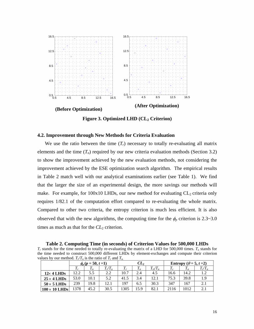
shown in Figure 3, before optimization, the initial LHD is a random design with good
one-dimensional projective property but not so good space-filling property. After
optimization, the projective property is maintained while the space filling property is
much improved.
16
(Before Optimization) (After Optimization)
Figure 3. Optimized LHD (CL2 Criterion)
4.2. Improvement through New Methods for Criteria Evaluation
We use the ratio between the time (Tr) necessary to totally re-evaluating all matrix
elements and the time (Tn) required by our new criteria evaluation methods (Section 3.2)
to show the improvement achieved by the new evaluation methods, not considering the
improvement achieved by the ESE optimization search algorithm. The empirical results
in Table 2 match well with our analytical examinations earlier (see Table 1). We find
that the larger the size of an experimental design, the more savings our methods will
make. For example, for 100x10 LHDs, our new method for evaluating CL2 criteria only
requires 1/82.1 of the computation effort compared to re-evaluating the whole matrix.
Compared to other two criteria, the entropy criterion is much less efficient. It is also
observed that with the new algorithms, the computing time for the φp criterion is 2.3~3.0
times as much as that for the CL2 criterion.
Table 2. Computing Time (in seconds) of Criterion Values for 500,000 LHDs Tr stands for the time needed to totally re-evaluating the matrix of a LHD for 500,000 times. Tn stands for the time needed to construct 500,000 different LHDs by element-exchanges and compute their criterion values by our method. Tr/Tn is the ratio of Tr and Tn.
φp (p = 50, t =1) CL2 Entropy (θ = 5, t =2) Tr Tn Tr/Tn Tr Tn Trt/Tn Tr Tn Tr/Tn 12× 4 LHDs 12.2 5.5 2.2 10.7 2.4 4.5 16.6 14.2 1.2 25 × 4 LHDs 53.0 10.1 5.2 41.5 3.4 12.1 75.3 39.8 1.9 50 × 5 LHDs 239 19.8 12.1 197 6.5 30.3 347 167 2.1
100 × 10 LHDs 1378 45.2 30.5 1305 15.9 82.1 2116 1012 2.1
0.5 4.5 8.5 12.5 16.50.5
4.5
8.5
12.5
16.5
0.5 4.5 8.5 12.5 16.50.5
4.5
8.5
12.5
16.5
17
4.3. Improvement through the ESE Search Algorithm
To verify the improved efficiency of the proposed ESE search algorithm, we compare
its performance with two other well known search algorithms, CP and SA, used
respectively by Li and Wu (1997) and Morris and Mitchell (1995) for optimizing DOEs.
In all test runs, the optimality criterion is evaluated using our proposed methods (Section
3.2) instead of re-evaluating all matrix elements. The tests are conducted on two sets of
LHDs of relatively small sizes, i.e., 12×4 and 25×4, and two sets of LHDs of relatively
large sizes, i.e., 50×5 and 100×10. As randomness is involved in all constructing
algorithms, we repeat the same test 100 times starting from different initial LHDs. On
each set of LHDs, two types of comparison are made, i.e.,
Type-I: Comparing the performance of ESE with that of SA and CP in terms of the
average of criterion values of optimal designs with nearly the same numbers of
exchanges. This group of tests for ESE is denoted as ESE (I)
Type-II: Comparing the efficiency of ESE with that of SA and CP in terms of
numbers of exchanges needed for ESE to achieve optimal designs with the average of
criterion values slightly better than that of SA or CP. This group of tests for ESE is
denoted as ESE (II)
In both types of comparison, t-test is used to statistically compare the average
criterion value of the optimal designs generated by ESE with those generated by SA or
CP. The p-value is used to measure the level at which the observed difference (< 0)
between the average criterion values is statistically significant. We use a tighter standard
that the p-value should be smaller than 0.001%. For type-I comparison, this standard is
not that critical since virtually all the p-values in the comparison are much smaller than
0.001%; for type-II comparison, however, this standard is used to judge whether optimal
designs generated by ESE are close to but still statistically significantly better than those
generated by SA or CP.
4.3.1. Results of Small Sizes of Designs
For small-sized LHDs, relatively large number of exchanges is affordable. For
example, with 2,865,600 exchanges, it takes ESE about 57 seconds to construct an
optimal 25×4 LHDs based on the φp criterion. The tests for small-sized problems are
18
therefore focused on the capability of moving away from locally optimal designs and
finding better experimental designs given a large number of exchanges.
The results of using the φp criterion are shown in Table 4. For each algorithm, two
sets of tests with different numbers of exchanges are conducted. For SA, the two sets of
tests correspond to two different values for cooling factor α suggested by Morris and
Mitchell (1995), i.e., α = 0.90 (faster cooling) and 0.95 (slower cooling), respectively. In
a particular set of tests, the numbers of exchanges of SA for constructing optimal designs
will differ test by test. For instance, for 12×4 LHD and α = 0.95, the numbers of
exchanges could be anywhere between 362,384 and 1,192,482. The numbers of
exchanges of SA shown in the table are the average numbers. CP is terminated at a cycle
number Ns, which is selected so that the average number of exchanges is close to that of
SA. The numbers of exchanges shown are also the average of 100 tests. The results of
SA are used to determine when to stop ESE.
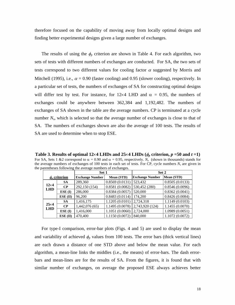
Table 3. Results of optimal 12×4 LHDs and 25×4 LHDs (φp criterion, p =50 and t =1) For SA, Sets 1 &2 correspond to α = 0.90 and α = 0.95, respectively. Ne (shown in thousands) stands for the average numbers of exchanges of 100 tests in each set of tests. For CP, cycle numbers Ns are given in the parentheses following the average numbers of exchanges.
Set 1 Set 2 φp criterion Exchange Number Mean (STD) Exchange Number Mean (STD)
SA 289,360 0.8569 (0.0131) 523,432 0.8505 (0.0133) CP 292,150 (154) 0.8581 (0.0082) 530,452 (280) 0.8546 (0.0096)
ESE (I) 286,000 0.8384 (0.0057) 520,000 0.8362 (0.0041)
12×4 LHD
ESE (II) 96,200 0.8483 (0.0114) 174,200 0.8426 (0.0084)
SA 1,416,175 1.1205 (0.0101) 2,724,318 1.1149 (0.0103) CP 1,442,076 (65) 1.1495 (0.0078) 2,743,920 (124) 1.1455 (0.0070)
ESE (I) 1,416,000 1.1051 (0.0060) 2,724,000 1.0989 (0.0051)
25×4 LHD
ESE (II) 470,400 1.1150 (0.0072) 840,000 1.1072 (0.0072)
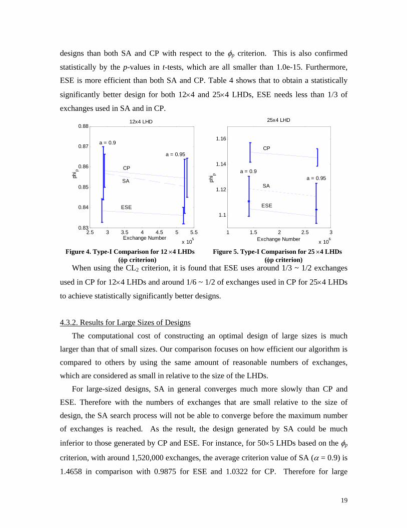
For type-I comparison, error-bar plots (Figs. 4 and 5) are used to display the mean
and variability of achieved φp values from 100 tests. The error bars (thick vertical lines)
are each drawn a distance of one STD above and below the mean value. For each
algorithm, a mean-line links the middles (i.e., the means) of error-bars. The dash error-
bars and mean-lines are for the results of SA. From the figures, it is found that with
similar number of exchanges, on average the proposed ESE always achieves better
19
designs than both SA and CP with respect to the φp criterion. This is also confirmed
statistically by the p-values in t-tests, which are all smaller than 1.0e-15. Furthermore,
ESE is more efficient than both SA and CP. Table 4 shows that to obtain a statistically
significantly better design for both 12×4 and 25×4 LHDs, ESE needs less than 1/3 of
exchanges used in SA and in CP.
2.5 3 3.5 4 4.5 5 5.5
x 105
0.83
0.84
0.85
0.86
0.87
0.88
Exchange Number
phi p
12x4 LHD
CP
ESE
SA
a = 0.9
a = 0.95
1 1.5 2 2.5 3
x 106
1.1
1.12
1.14
1.16
25x4 LHD
Exchange Number
phi p
CP
ESE
SA
a = 0.9 a = 0.95
Figure 4. Type-I Comparison for 12 ×4 LHDs Figure 5. Type-I Comparison for 25 ×4 LHDs
(φp criterion) (φp criterion) When using the CL2 criterion, it is found that ESE uses around 1/3 ~ 1/2 exchanges
used in CP for 12×4 LHDs and around 1/6 ~ 1/2 of exchanges used in CP for 25×4 LHDs
to achieve statistically significantly better designs.
4.3.2. Results for Large Sizes of Designs
The computational cost of constructing an optimal design of large sizes is much
larger than that of small sizes. Our comparison focuses on how efficient our algorithm is
compared to others by using the same amount of reasonable numbers of exchanges,
which are considered as small in relative to the size of the LHDs.
For large-sized designs, SA in general converges much more slowly than CP and
ESE. Therefore with the numbers of exchanges that are small relative to the size of
design, the SA search process will not be able to converge before the maximum number
of exchanges is reached. As the result, the design generated by SA could be much
inferior to those generated by CP and ESE. For instance, for 50×5 LHDs based on the φp
criterion, with around 1,520,000 exchanges, the average criterion value of SA (α = 0.9) is
1.4658 in comparison with 0.9875 for ESE and 1.0322 for CP. Therefore for large

20
problems, SA may not be suitable since it needs excessive numbers of exchanges. Our
test for large-sized designs only focuses on CP and ESE.
CP provides baselines for determining when to stop ESE in both types of
comparisons. For large-sized problems, the computational cost could be too high for CP
to even finish a single cycle. For instance, a single cycle of CP for 100×10 LHD with φp
criterion could take 31,482,000 exchanges (2,758 seconds). Therefore, the tests of CP for
large-sized LHDs have been restricted to at most several cycles for 50×5 LHDs and one
cycle for 100×10 LHDs. Table 5 shows the maximum numbers of exchanges and the
computing time. From the table we find that the computing time has been close to merely
several minutes (if not seconds).
Table 4. Maximum Exchange Number and Computing Time for Constructing Optimal LHDs
φp CL2 Max Exchange
Number Max Computing Time (seconds)
Max Exchange Number
Max Computing Time (seconds)
50×5 LHDs 1,945,000 77 2,960,000 35 100×10 LHDs 2,500,000 219 7,685,000 198
As shown in Table 5, for each algorithm, three sets of tests with different numbers of
exchanges are performed. For 50×5 LHDs, the numbers of exchanges of the first set of
tests are not sufficient to finish one cycle; the second set of tests involves exactly one
cycle and the numbers of exchanges are the average of the 100 tests; likewise, the third
set of tests involves exactly 5 cycles. For 100×10 LHDs, even though large numbers of
exchanges are used for CP in all three sets of tests, they are not sufficient to finish the
first cycle. Table 5. Test Results of optimal 50×5 LHDs and 100×10 LHDs based on φp criterion (p =50, t =1) For CP, the cycle numbers are provided in the parentheses following the exchange numbers. If there are no cycle numbers marked, it means that CP is stopped within the first cycle
Set 1 Set 2 Set 3 φp criterion Exchange
Number Mean (STD) Exchange Number Mean (STD) Exchange
Number Mean (STD)
CP 61,250 1.1564 (0.0121) 403,638 (1) 1.0420 (0.0097) 1,947,811
(5) 1.0311 (0.0068)
ESE (I) 60,000 1.0486 (0.0072) 400,000 1.0076 (0.0059) 1,945,000 0.9850 (0.0038)
50×5 LHD
ESE (II) 10,000 1.1264 (0.0099) 80,000 1.0348 (0.0069) 110,000 1.0248 (0.0063)
CP 297,000 0.5381 (0.0044) 544,500 0.5059 (0.0024) 2,524,500 0.4660 (0.0014)ESE (I) 280,000 0.4562 (0.0012) 500,000 0.4525 (0.0014) 2,500,000 0.4440 (0.0010)
100×10 LHD
ESE (II) 10,000 0.5214 (0.0031) 20,000 0.4996 (0.0025) 140,000 0.4634 (0.0015)
21
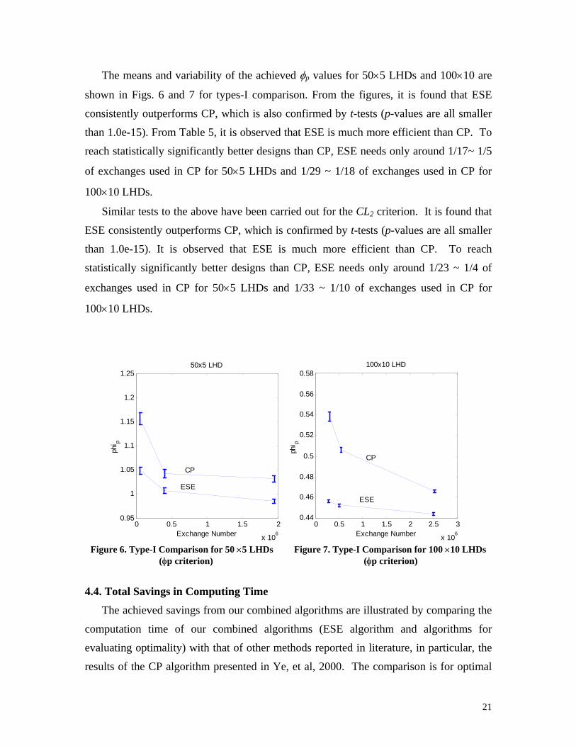
The means and variability of the achieved φp values for 50×5 LHDs and 100×10 are
shown in Figs. 6 and 7 for types-I comparison. From the figures, it is found that ESE
consistently outperforms CP, which is also confirmed by t-tests (p-values are all smaller
than 1.0e-15). From Table 5, it is observed that ESE is much more efficient than CP. To
reach statistically significantly better designs than CP, ESE needs only around 1/17~ 1/5
of exchanges used in CP for 50×5 LHDs and 1/29 ~ 1/18 of exchanges used in CP for
100×10 LHDs.
Similar tests to the above have been carried out for the CL2 criterion. It is found that
ESE consistently outperforms CP, which is confirmed by t-tests (p-values are all smaller
than 1.0e-15). It is observed that ESE is much more efficient than CP. To reach
statistically significantly better designs than CP, ESE needs only around 1/23 ~ 1/4 of
exchanges used in CP for 50×5 LHDs and 1/33 ~ 1/10 of exchanges used in CP for
100×10 LHDs.
0 0.5 1 1.5 2
x 106
0.95
1
1.05
1.1
1.15
1.2
1.2550x5 LHD
Exchange Number
phi p
CP
ESE
0 0.5 1 1.5 2 2.5 3
x 106
0.44
0.46
0.48
0.5
0.52
0.54
0.56
0.58100x10 LHD
Exchange Number
phi p
CP
ESE
Figure 6. Type-I Comparison for 50 ×5 LHDs Figure 7. Type-I Comparison for 100 ×10 LHDs
(φp criterion) (φp criterion)
4.4. Total Savings in Computing Time
The achieved savings from our combined algorithms are illustrated by comparing the
computation time of our combined algorithms (ESE algorithm and algorithms for
evaluating optimality) with that of other methods reported in literature, in particular, the
results of the CP algorithm presented in Ye, et al, 2000. The comparison is for optimal
22
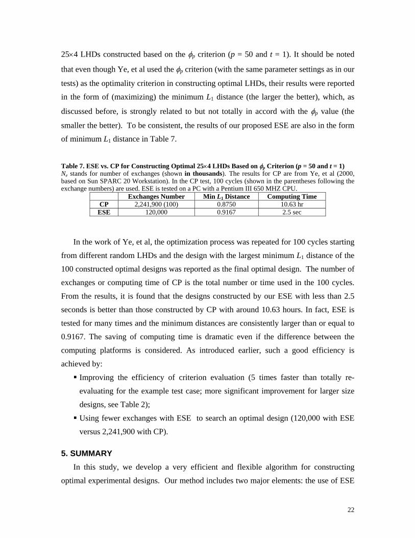
25×4 LHDs constructed based on the φp criterion (p = 50 and t = 1). It should be noted
that even though Ye, et al used the φp criterion (with the same parameter settings as in our
tests) as the optimality criterion in constructing optimal LHDs, their results were reported
in the form of (maximizing) the minimum L1 distance (the larger the better), which, as
discussed before, is strongly related to but not totally in accord with the φp value (the
smaller the better). To be consistent, the results of our proposed ESE are also in the form
of minimum L1 distance in Table 7.
Table 7. ESE vs. CP for Constructing Optimal 25×4 LHDs Based on φp Criterion (p = 50 and t = 1) Ne stands for number of exchanges (shown in thousands). The results for CP are from Ye, et al (2000, based on Sun SPARC 20 Workstation). In the CP test, 100 cycles (shown in the parentheses following the exchange numbers) are used. ESE is tested on a PC with a Pentium III 650 MHZ CPU.
Exchanges Number Min L1 Distance Computing Time CP 2,241,900 (100) 0.8750 10.63 hr
ESE 120,000 0.9167 2.5 sec
In the work of Ye, et al, the optimization process was repeated for 100 cycles starting
from different random LHDs and the design with the largest minimum L1 distance of the
100 constructed optimal designs was reported as the final optimal design. The number of
exchanges or computing time of CP is the total number or time used in the 100 cycles.
From the results, it is found that the designs constructed by our ESE with less than 2.5
seconds is better than those constructed by CP with around 10.63 hours. In fact, ESE is
tested for many times and the minimum distances are consistently larger than or equal to
0.9167. The saving of computing time is dramatic even if the difference between the
computing platforms is considered. As introduced earlier, such a good efficiency is
achieved by:
Improving the efficiency of criterion evaluation (5 times faster than totally re-
evaluating for the example test case; more significant improvement for larger size
designs, see Table 2);
Using fewer exchanges with ESE to search an optimal design (120,000 with ESE
versus 2,241,900 with CP).
5. SUMMARY In this study, we develop a very efficient and flexible algorithm for constructing
optimal experimental designs. Our method includes two major elements: the use of ESE
23
algorithm for controlling the search process and the employment of efficient methods for
evaluating the optimality criteria. Our proposed algorithm has shown great efficiency
compared to some algorithms in the literature. Specifically, it has cut the computation
time from hours to minutes and seconds, which makes the just-in-time generation of large
size optimal designs possible. In comparison, we have the following observations:
• With the same number of exchanges, the optimal designs generated by ESE is
generally better than those generated by SA and CP.
• To obtain a design statistically significantly better than those generated by SA and
CP, ESE needs far less number of exchanges (typically around 1/6 ~ 1/2 of
exchanges needed by SA or CP for small-sized designs and 1/33~ 1/4 of exchanges
needed by CP for large-sized designs).
• For small-size problems (a relatively large number of exchanges are affordable),
SA often has better performance than CP. However, for large-size problems, SA
may converge very slowly and require a tremendous number of exchanges.
While our focus in this paper is on optimizing LHDs, the ESE algorithm can be used
to optimize other classes of designs such as OAs and OLs. Furthermore, while the
algorithm works on the φp criterion, the entropy criterion, and the CL2 criterion, it can be
conveniently extended to other optimality criteria.
ACKNOWLEDGMENTS NSF grants 0099775 and 0217702 are acknowledged. The authors would like to
thank the referees for their valuable inputs to improve the presentation of the paper.
REFERENCES Fang, K.T., Lin, D. K., Winker, J. P., Zhang, Y., 2000, Uniform Design: Theory and
Application, Technometrics, V42 n3, 237-248
Fang, K.T., Ma, C.X. and Winker, P., 2002, Centered L2-discrepancy of random
sampling and Latin hypercube design, and construction of uniform designs, Mathematics
of Computation, 71, 275-296.
Hickernell, F. J., 1998, “A generalized discrepancy and quadrature error bound”,
Mathematics of Computation, 67, 299-322.
Hedayat, A.S., Stufken, J., Sloane N. J., 1999, Orthogonal Arrays: Theory and
Applications, Springer-Verlag New York.
24
Jin, R., 2003, Investigations and Enhancements of Metamodeling Techniques in
Engineering Design, Ph.D Thesis, Univ. of Illinois at Chicago.
Johnson, M. and Moore, L. and Ylvisaker, D., 1990, “Minimax and maximin distance
designs”, Journal of Statistical Planning and Inference, 26, 131-148.
Koehler, J.R. and Owen, A.B., 1996, Computer experiments, in Ghosh, S.and Rao,
C.R., eds, Handbook of Statistics, 13, 261 –308, Elsevier Science, New York.
Li W. and Nachtsheim C.J., 2000, Model-Robust Factorial Designs, Technometrics,
Vol. 42, 345-352.
Li, W. and Wu, C. F. J., 1997, Columnwise-Pairwise Algorithms With Applications
to the Construction of Supersaturated Designs, Technometrics , Vol. 39, 171-179.
McKay, M.D., Beckman, R.J. and Conover, W.J., 1979, “A comparison of three
methods for selecting values of input variables in the analysis of output from a computer
code”, Technometrics, 21(2), 239-45.
Morris, M.D., Mitchell, T.J., 1995, Exploratory Designs for Computational
Experiments, Journal of statistical planning and inference, 43, 381-402.
Owen, A.B., 1992, Orthogonal arrays for computer experiments, integration and
visualization, Statistical Sinica, v2, n2, 439-452.
Park, J.-S., 1994, Optimal Latin-hypercube designs for computer experiments,
Journal of Statistical Planning and Inference, 39, 95-111.
Press, W.H., Teukoisky, S.A., Vetterling, W.T., Flannery, B.P., 1997, Numerical
Recipes in C: the Art of Scientific Computing, Cambridge U. Press, 332~338.
Saab, Y.G., Rao, Y.B., 1991, Combinatorial optimization by stochastic evolution,
IEEE Transactions on Computer-aided Design, v10, n4, 525-535.
Shannon, C.E., 1948, A mathematical theory of communication, Bell System
Technical Journal, 27:379-423, 623-656.
Tang, Boxin, Orthogonal array-based Latin Hypercubes, 1993, Journal of the
American Statistical Association, v88, n424, 1392~1397
Winker, P. and Fang, K. T., 1998, Optimal U-type design, in Monte Carlo and Quasi-
Monte Carlo Methods 1996, eds. by H. Niederreiter, P. Zinterhof and P. Hellekalek,
Springer, 436-448.

25
Ye, K. Q., Li, W., Sudjianto, A., 2000, Algorithmic construction of optimal
symmetric Latin hypercube designs, Journal of Statistical Planning and Inference, 90,
145-159.