an efficient way to perform the assembly of finite element · pdf fileelement matrices in...
TRANSCRIPT

arX
iv:1
305.
3122
v1 [
cs.N
A]
14
May
201
3
ISS
N02
49-6
399
ISR
NIN
RIA
/RR
--83
05--
FR
+E
NG
RESEARCHREPORT
N° 8305May 2013
Project-Teams Pomdapi
An efficient way toperform the assembly offinite element matrices inMatlab and OctaveFrançois Cuvelier, Caroline Japhet , Gilles Scarella


RESEARCH CENTREPARIS – ROCQUENCOURT
Domaine de Voluceau, - Rocquencourt
B.P. 105 - 78153 Le Chesnay Cedex
An efficient way to perform the assembly of
finite element matrices in Matlab and Octave
François Cuvelier ˚, Caroline Japhet ˚ §, Gilles Scarella˚
Project-Teams Pomdapi
Research Report n° 8305 — May 2013 — 37 pages
Abstract: We describe different optimization techniques to perform the assembly of finiteelement matrices in Matlab and Octave, from the standard approach to recent vectorized ones,without any low level language used. We finally obtain a simple and efficient vectorized algorithmable to compete in performance with dedicated software such as FreeFEM++. The principle ofthis assembly algorithm is general, we present it for different matrices in the P1 finite elementscase and in linear elasticity. We present numerical results which illustrate the computational costsof the different approaches.
Key-words: P1 finite elements, matrix assembly, vectorization, linear elasticity, Matlab, Octave
This work was partially supported by the GNR MoMaS (PACEN/CNRS, ANDRA, BRGM,CEA, EDF, IRSN)
˚ Université Paris 13, Sorbonne Paris Cité, LAGA, CNRS UMR 7539, 99 Av-enue J-B Clément, 93430 Villetaneuse, France, Emails: [email protected],
[email protected], [email protected]§ INRIA Paris-Rocquencourt, project-team Pomdapi, 78153 Le Chesnay Cedex, France
Email:[email protected]

Optimisation de l’assemblage de matrices éléments
finis sous Matlab et OctaveRésumé : L’objectif est de décrire différentes techniques d’optimisation, sousMatlab/Octave, de routines d’assemblage de matrices éléments finis, en partant del’approche classique jusqu’aux plus récentes vectorisées, sans utiliser de langage debas niveau. On aboutit au final à une version vectorisée rivalisant, en terme deperformance, avec des logiciels dédiés tels que FreeFEM++. Les descriptions desdifférentes méthodes d’assemblage étant génériques, on les présente pour différentesmatrices dans le cadre des éléments finis P1´Lagrange en dimension 2 et en élasticitélinéaire. Des résultats numériques sont donnés pour illustrer les temps calculs desméthodes proposées.
Mots-clés : éléments finis P1, assemblage de matrices, vectorisation, élasticitélinéaire, Matlab, Octave
An efficient way to perform the assembly of finite element matrices in Matlab and Octave3
1. Introduction. Usually, finite elements methods [4, 14] are used to solve par-tial differential equations (PDEs) occurring in many applications such as mechanics,fluid dynamics and computational electromagnetics. These methods are based on adiscretization of a weak formulation of the PDEs and need the assembly of large sparsematrices (e.g. mass or stiffness matrices). They enable complex geometries and vari-ous boundary conditions and they may be coupled with other discretizations, using aweak coupling between different subdomains with nonconforming meshes [1]. Solvingaccurately these problems requires meshes containing a large number of elements andthus the assembly of large sparse matrices.
Matlab [16] and GNU Octave [11] are efficient numerical computing softwares us-ing matrix-based language for teaching or industry calculations. However, the classicalassembly algorithms (see for example [5, 15]) basically implemented in Matlab/Octaveare much less efficient than when implemented with other languages.
In [8] Section 10, T. Davis describes different assembly techniques applied torandom matrices of finite element type, while the classical matrices are not treated.A first vectorization technique is proposed in [8]. Other more efficient algorithmshave been proposed recently in [2, 3, 12, 17]. More precisely, in [12], a vectorizationis proposed, based on the permutation of two local loops with the one through theelements. This more formal technique allows to easily assemble different matrices,from a reference element by affine transformation and by using a numerical integration.In [17], the implementation is based on extending element operations on arrays intooperations on arrays of matrices, calling it a matrix-array operation, where the arrayelements are matrices rather than scalars, and the operations are defined by the rulesof linear algebra. Thanks to these new tools and a quadrature formula, differentmatrices are computed without any loop. In [3], L. Chen builds vectorially the ninesparse matrices corresponding to the nine elements of the element matrix and addsthem to obtain the global matrix.
In this paper we present an optimization approach, in Matlab/Octave, using avectorization of the algorithm. This finite element assembly code is entirely vectorized(without loop) and without any quadrature formula. Our vectorization is close to theone proposed in [2], with a full vectorization of the arrays of indices.
Due to the length of the paper, we restrict ourselves to P1 Lagrange finite elementsin 2D with an extension to linear elasticity. Our method extends easily to the Pk finiteelements case, k ě 2, and in 3D, see [7]. We compare the performances of this codewith the ones obtained with the standard algorithm and with those proposed in [2,3, 12, 17]. We also show that this implementation is able to compete in performancewith dedicated software such as FreeFEM++ [13]. All the computations are done onour reference computer1 with the releases R2012b for Matlab, 3.6.3 for Octave and3.20 for FreeFEM++. The entire Matlab/Octave code may be found in [6]. TheMatlab codes are fully compatible with Octave.
The remainder of this paper is organized as follows: in Section 2 we give thenotations associated to the mesh and we define three finite element matrices. Then,in Section 3 we recall the classical algorithm to perform the assembly of these matricesand show its inefficiency compared to FreeFEM++. This is due to the storage of sparse
˚Université Paris 13, Sorbonne Paris Cité, LAGA, CNRS UMR 7539, 99 Avenue J-B Clément,93430 Villetaneuse, France ([email protected], [email protected],[email protected])
§INRIA Paris-Rocquencourt, project-team Pomdapi, 78153 Le Chesnay Cedex, France12 x Intel Xeon E5645 (6 cores) at 2.40Ghz, 32Go RAM, supported by GNR MoMaS
RR n° 8305

4 F. Cuvelier, C. Japhet, G. Scarella
matrices in Matlab/Octave as explained in Section 4. In Section 5 we give a method tobest use Matlab/Octave sparse function, the “optimized version 1”, suggested in [8].Then, in Section 6 we present a new vectorization approach, the “optimized version2”, and compare its performances to those obtained with FreeFEM++ and the codesgiven in [2, 3, 12, 17]. Finally, in Section 7, we present an extension to linear elasticity.The full listings of the routines used in the paper are given in Appendix B (see also[6]).
2. Notations. Let Ω be an open bounded subset of R2. It is provided with itsmesh Th (classical and locally conforming). We use a triangulation Ωh “
Ť
TkPThTk
of Ω (see Figure 2.1) described by :
name type dimension descriptionnq integer 1 number of verticesnme integer 1 number of elementsq double 2 ˆ nq array of vertices coordinates. qpν, jq is the ν-th coor-
dinate of the j-th vertex, ν P t1, 2u, j P t1, . . . , nqu.The j-th vertex will be also denoted by qj withqjx “ qp1, jq and qjy “ qp2, jq
me integer 3 ˆ nme connectivity array. mepβ, kq is the storage index ofthe β-th vertex of the k-th triangle, in the array q,for β P t1, 2, 3u and k P t1, . . . , nmeu
areas double 1 ˆ nme array of areas. areaspkq is the k-th triangle area,k P t1, . . . , nmeu
1
2
3
4
5
6
7
8
9
10
11
12
13
14
15
16
17
18
19
20
1
2
3
4
5 6
7
8
9
10
11 12
13
14
15
16
17
18
1920
21
22
23
24
25
26
1
2
34
5
6
7
8
9 10
11
12
Nodes number
Edges number
Triangles number
Fig. 2.1. Description of the mesh.
In this paper we will consider the assembly of the mass, weighted mass and stiffnessmatrices denoted by M, Mrws and S respectively. These matrices of size nq are sparse,and their coefficients are defined by
Mi,j “
ż
Ωh
ϕipqqϕjpqqdq, Mrwsi,j “
ż
Ωh
wpqqϕipqqϕjpqqdq, Si,j “
ż
Ωh
x∇ϕipqq,∇ϕjpqqy dq,
where ϕi are the usual P1 Lagrange basis functions, w is a function defined on Ω andx¨, ¨y is the usual scalar product in R2. More details are given in [5]. To assemble

An efficient way to perform the assembly of finite element matrices in Matlab and Octave 5
these matrices, one needs to compute its associated element matrix. On a triangle Twith local vertices q1, q2, q3 and area |T |, the element mass matrix is given by
MepT q “
|T |
12
¨
˝
2 1 1
1 2 1
1 1 2
˛
‚. (2.1)
Let wα “ wpqαq, @α P t1, . . . , 3u. The element weighted mass matrix is approximatedby
Me,rwspT q “
|T |
30
¨
˝
3w1 ` w2 ` w3 w1 ` w2 ` w3
2w1 ` w2
2` w3
w1 ` w2 ` w3
2w1 ` 3w2 ` w3
w1
2` w2 ` w3
w1 ` w2
2` w3
w1
2` w2 ` w3 w1 ` w2 ` 3w3
˛
‚. (2.2)
Denoting uuu “ q2 ´ q3, vvv “ q3 ´ q1 and www “ q1 ´ q2, the element stiffness matrix is
SepT q “
1
4|T |
¨
˝
xuuu,uuuy xuuu,vvvy xuuu,wwwyxvvv,uuuy xvvv,vvvy xvvv,wwwyxwww,uuuy xwww,vvvy xwww,wwwy
˛
‚. (2.3)
The listings of the routines to compute the previous element matrices are given in Ap-pendix B.1 We now give the classical assembly algorithm using these element matriceswith a loop through the triangles.
3. The classical algorithm. We describe the assembly of a given nqˆnq matrixM from its associated 3 ˆ 3 element matrix E. We denote by “ElemMat” the routinewhich computes the element matrix E.
Listing 1
Classical matrix assembly code in Matlab/Octave
M=sparse (nq , nq ) ;for k=1:nme
E=ElemMat( areas ( k ) , . . . ) ;for i l =1:3
i=me( i l , k ) ;for j l =1:3
j=me( j l , k ) ;M( i , j )=M( i , j )+E( i l , j l ) ;
end
end
end
We aim to compare the performances of this code (see Appendix B.2 for the completelistings) with those obtained with FreeFEM++ [13]. The FreeFEM++ commandsto build the mass, weighted mass and stiffness matrices are given in Listing 2. OnFigure 3.1, we show the computation times (in seconds) versus the number of verticesnq of the mesh (unit disk), for the classical assembly and FreeFEM++ codes. Thevalues of the computation times are given in Appendix A.1. We observe that thecomplexity is Opn2qq (quadratic) for the Matlab/Octave codes, while the complexityseems to be Opnqq (linear) for FreeFEM++.

6 F. Cuvelier, C. Japhet, G. Scarella
Listing 2
Matrix assembly code in FreeFEM++
mesh Th ( . . . ) ;f e sp ac e Vh(Th,P1) ; // P1 FE-spacevar f vMass (u , v )= int2d (Th) ( u∗v ) ;var f vMassW (u , v )= int2d (Th) ( w∗u∗v) ;var f v S t i f f (u , v )= int2d (Th) ( dx (u ) ∗dx(v )
+ dy(u) ∗dy(v ) ) ;
matrix M= vMass (Vh,Vh) ; // Mass matrix assemblymatrix Mw = vMassW(Vh,Vh) ; // Weighted mass matrix assemblymatrix S = v S t i f f (Vh,Vh) ; // Stiffness matrix assembly
103
104
105
106
10−2
10−1
100
101
102
103
104
105
nq
time
(s)
MatlabOctaveFreeFEM++O(n
q)
O(nq2)
103
104
105
106
10−2
10−1
100
101
102
103
104
105
nq
time
(s)
MatlabOctaveFreeFEM++O(n
q)
O(nq2)
103
104
105
106
10−2
10−1
100
101
102
103
104
105
nq
time
(s)
MatlabOctaveFreeFEM++O(n
q)
O(nq2)
Fig. 3.1. Comparison of the classical matrix assembly code in Matlab/Octave withFreeFEM++, for the mass (top left), weighted mass (top right) and stiffness (bottom) matrices.
We have surprisingly observed that the Matlab performances may be improved usingan older Matlab release (see Appendix C)
Our objective is to propose optimizations of the classical code that lead to more ef-ficient codes with computational costs comparable to those obtained with FreeFEM++.A first improvement of the classical algorithm (Listing 1) is to vectorize the two localloops, see Listing 3 (the complete listings are given in Appendix B.3).

An efficient way to perform the assembly of finite element matrices in Matlab and Octave 7
Listing 3
Optimized matrix assembly code - version 0
M=sparse (nq , nq ) ;for k=1:nme
I=me( : , k ) ;M( I , I )=M( I , I )+ElemMat( areas (k ) , . . . ) ;
end
However the complexity of this algorithm is still quadratic (i.e. Opn2qq).In the next section, we explain the storage of sparse matrices in Matlab/Octave
in order to justify this lack of efficiency.
4. Sparse matrices storage. In Matlab/Octave, a sparse matrix A P MM,NpRq,with nnz non-zeros elements, is stored with CSC (Compressed Sparse Column) formatusing the following three arrays:
aap1 : nnzq : which contains the nnz non-zeros elements of A stored column-wise,iap1 : nnzq : which contains the row numbers of the elements stored in aa,
jap1 : N ` 1q : which allows to find the elements of a column of A, with the infor-mation that the first non-zero element of the column k of A is in the japkq-thposition in the array aa. We have jap1q “ 1 and japN ` 1q “ nnz ` 1.
For example, with the matrix
A “
¨
˝
1. 0. 0. 6.
0. 5. 0. 4.
0. 1. 2. 0.
˛
‚,
we have M “ 3, N “ 4, nnz “ 6 and
aa 1. 5. 1. 2. 6. 4.
ia 1 2 3 3 1 2
ja 1 2 4 5 7
The first non-zero element in column k “ 3 of A is 2, the position of this number inaa is 4, thus jap3q “ 4.
We now describe the operations to be done on the arrays aa, ia and ja if wemodify the matrix A by taking Ap1, 2q “ 8. It becomes
A “
¨
˝
1. 8. 0. 6.
0. 5. 0. 4.
0. 1. 2. 0.
˛
‚.
In this case, a zero element of A has been replaced by the non-zero value 8 which mustbe stored in the arrays while no space is provided. We suppose that the arrays aresufficiently large (to avoid memory space problems), we must then shift one cell allthe values in the arrays aa and ia from the third position and then copy the value 8
in aap3q and the value 1 (row number) in iap3q :
aa 1. 8. 5. 1. 2. 6. 4.
ia 1 1 2 3 3 1 2

8 F. Cuvelier, C. Japhet, G. Scarella
For the array ja, we increment of 1 the values after the position 2 :
ja 1 2 5 6 8
The repetition of these operations is expensive upon assembly of the matrix in theprevious codes. Moreover, we haven’t considered dynamic reallocation problems thatmay also occur.
We now present the optimized version 1 of the code that will allow to improvethe performance of the classical code.
5. Optimized matrix assembly - version 1 (OptV1). We will use the fol-lowing call of the sparse Matlab function:
M = sparse(I,J,K,m,n);
This command returns a sparse matrix M of size m ˆ n such that M(I(k),J(k)) = K(k).The vectors I, J and K have the same length. The zero elements of K are not takeninto account and the elements of K having the same indices in I and J are summed.
The idea is to create three global 1d-arrays IIIg, JJJg and KKKg allowing the storageof the element matrices as well as the position of their elements in the global matrix.The length of each array is 9nme. Once these arrays are created, the matrix assemblyis obtained with the command
M = sparse(Ig,Jg,Kg,nq,nq);
To create these three arrays, we first define three local arrays KKKek, III
ek and JJJe
k ofnine elements obtained from a generic element matrix EpTkq of dimension 3 :
KKKek : elements of the matrix EpTkq stored column-wise,
IIIek : global row indices associated to the elements stored in KKKek,
JJJek : global column indices associated to the elements stored in KKKe
k.
We have chosen a column-wise numbering for 1d-arrays in Matlab/Octave implemen-tation, but for representation convenience we draw them in line format,
EpTkq “
¨
˚
˝
ek1,1 ek1,2 ek1,3ek2,1 ek2,2 ek2,3ek3,1 ek3,2 ek3,3
˛
‹
‚ùñ
KKKek : ek1,1 ek2,1 ek3,1 ek1,2 ek2,2 ek3,2 ek1,3 ek2,3 ek3,3
IIIek : ik1 ik2 ik3 ik1 ik2 ik3 ik1 ik2 ik3
JJJek : ik1 ik1 ik1 ik2 ik2 ik2 ik3 ik3 ik3
with ik1 “ mep1, kq, ik2 “ mep2, kq, ik3 “ mep3, kq.To create the three arrays KKKe
k, IIIek and JJJe
k, in Matlab/Octave, one can use thefollowing commands :
E = ElemMat( areas ( k ) , . . . ) ; % E : 3´by´3 matrixKe = E ( : ) ; % Ke : 9´by´1 matrixI e = me( [ 1 2 3 1 2 3 1 2 3 ] , k ) ; % Ie : 9´by´1 matrixJe = me( [ 1 1 1 2 2 2 3 3 3 ] , k ) ; % Je : 9´by´1 matrix
From these arrays, it is then possible to build the three global arrays IIIg, JJJg andKKKg, of size 9nme ˆ 1 defined by : @k P t1, . . . , nmeu , @il P t1, . . . , 9u,
KKKgp9pk ´ 1q ` ilq “ KKKekpilq,
IIIgp9pk ´ 1q ` ilq “ IIIekpilq,
JJJgp9pk ´ 1q ` ilq “ JJJekpilq.
On Figure 5.1, we show the insertion of the local array KKKek into the global 1d-array
KKKg, and, for representation convenience, we draw them in line format. We make thesame operation for the two other arrays.

An efficient way to perform the assembly of finite element matrices in Matlab and Octave 9
Kek
KKKg1 2 3 4 5 6 7 8 9 9
pk´1
q`1
9pk
´1
q`9
9pn
me
´1
q`9
9pn
me
´1
q`1
1 2 3 4 5 6 7 8 9
ek1,1 ek2,1 e
k3,1 e
k1,2 e
k2,2 e
k3,2 e
k1,3 e
k2,3 e
k3,3
ek1,1 ek2,1 e
k3,1 e
k1,2 e
k2,2 e
k3,2 e
k1,3 e
k2,3 e
k3,3
Fig. 5.1. Insertion of an element matrix in the global array - Version 1
We give in Listing 4 the Matlab/Octave associated code where the global vectorsIIIg, JJJg and KKKg are stored column-wise. The complete listings and the values of thecomputation times are given in Appendices B.4 and A.3 respectively. On Figure 5.2,we show the computation times of the Matlab, Octave and FreeFEM++ codes versusthe number of vertices of the mesh (unit disk). The complexity of the Matlab/Octavecodes seems now linear (i.e. Opnqq) as for FreeFEM++. However, FreeFEM++ isstill much more faster than Matlab/Octave (about a factor 5 for the mass matrix, 6.5for the weighted mass matrix and 12.5 for the stiffness matrix, in Matlab).
104
105
106
107
10−2
10−1
100
101
102
103
104
nq
time
(s)
MatlabOctaveFreeFEM++O(n
q)
O(nq2)
104
105
106
107
10−2
10−1
100
101
102
103
104
nq
time
(s)
Matlab
Octave
FreeFEM++O(n
q)
O(nq2)
104
105
106
107
10−2
10−1
100
101
102
103
104
nq
time
(s)
Matlab
Octave
FreeFEM++O(n
q)
O(nq2)
Fig. 5.2. Comparison of the matrix assembly codes : OptV1 in Matlab/Octave andFreeFEM++, for the mass (top left), weighted mass (top right) and stiffness (bottom) matrices.

10 F. Cuvelier, C. Japhet, G. Scarella
Listing 4
Optimized matrix assembly code - version 1
Ig=zeros (9∗nme , 1 ) ; Jg=zeros (9∗nme , 1 ) ;Kg=zeros (9∗nme , 1 ) ;i i =[1 2 3 1 2 3 1 2 3 ] ; j j =[1 1 1 2 2 2 3 3 3 ] ;kk=1:9 ;for k=1:nme
E=ElemMat( areas (k ) , . . . ) ;Ig ( kk)=me( i i , k ) ;Jg ( kk)=me( j j , k ) ;Kg( kk)=E ( : ) ;kk=kk+9;
end
M=sparse ( Ig , Jg ,Kg, nq , nq ) ;
To further improve the efficiency of the codes, we introduce now a second optimizedversion of the assembly algorithm.
6. Optimized matrix assembly - version 2 (OptV2). We present the opti-mized version 2 of the algorithm where no loop is used.
We define three 2d-arrays that allow to store all the element matrices as wellas their positions in the global matrix. We denote by Kg, Ig and Jg these 9-by-nme
arrays, defined @k P t1, . . . , nmeu , @il P t1, . . . , 9u by
Kgpil, kq “ KKKekpilq, Igpil, kq “ IIIekpilq, Jgpil, kq “ JJJe
kpilq.
The three local arraysKKKek, III
ek and JJJe
k are thus stored in the k-th column of the globalarrays Kg, Ig and Jg respectively.
A natural way to build these three arrays consists in using a loop through thetriangles Tk in which we insert the local arrays column-wise, see Figure 6.1. Oncethese arrays are determined, the matrix assembly is obtained with the Matlab/Octavecommand
M = sparse(Ig(:),Jg(:),Kg(:),nq,nq);
We remark that the matrices containing global indices Ig and Jg may be computed,in Matlab/Octave, without any loop. For the computation of these two matrices, onthe left we give the usual code and on the right the vectorized code :
Ig=zeros (9 ,nme ) ; Jg=zeros (9 ,nme ) ;for k=1:nme
Ig ( : , k)=me( [ 1 2 3 1 2 3 1 2 3 ] , k ) ;Jg ( : , k)=me( [ 1 1 1 2 2 2 3 3 3 ] , k ) ;
end
Ig=me( [ 1 2 3 1 2 3 1 2 3 ] , : ) ;Jg=me( [ 1 1 1 2 2 2 3 3 3 ] , : ) ;
Another way to present this computation, used and adapted in Section 7, is given by
Remark 6.1. Denoting Ik “ rmep1, kq, mep2, kq, mep3, kqs and
T “
¨
˝
I1p1q . . . Ikp1q . . . Inmep1q
I1p2q . . . Ikp2q . . . Inmep2q
I1p3q . . . Ikp3q . . . Inmep3q
˛
‚,
then, in that case T “ me, and Ig and Jg may be computed from T as follows:
i i =[1 1 1 ; 2 2 2 ; 3 3 3 ] ; j j=i i ’ ;I g=T( i i ( : ) , : ) ; Jg=T( j j ( : ) , : ) ;

An efficient way to perform the assembly of finite element matrices in Matlab and Octave 11
ek1,1 ek1,2 ek1,3
ek2,1 ek2,2 ek2,3
ek3,1 ek3,2 ek3,3
¨
˚
˚
˚
˚
˚
˚
˚
˚
˚
˚
˚
˝
˛
‹
‹
‹
‹
‹
‹
‹
‹
‹
‹
‹
‚
EpTkq
ek1,1
ek2,1
ek3,1
ek1,2
ek2,2
ek3,2
ek1,3
ek2,3
ek3,3
KKKek
ik1
ik2
ik3
ik1
ik2
ik3
ik1
ik2
ik3
IIIek
ik1
ik1
ik1
ik2
ik2
ik2
ik3
ik3
ik3
JJJek
Kg
ek1,1
ek2,1
ek3,1
ek1,2
ek2,2
ek3,2
ek1,3
ek2,3
ek3,3
1
2
3
4
5
6
7
8
9
1 2 . . . k . . . nme
Ig
ik1
ik2
ik3
ik1
ik2
ik3
ik1
ik2
ik3
1
2
3
4
5
6
7
8
9
1 2 . . . k . . . nme
Jg
ik1
ik1
ik1
ik2
ik2
ik2
ik3
ik3
ik3
1
2
3
4
5
6
7
8
9
1 2 . . . k . . . nme
Fig. 6.1. Insertion of an element matrix in the global array - Version 2
It remains to vectorize the computation of the 2d-array Kg. The usual code,corresponding to a column-wise computation, is :
Listing 5
Usual assembly (column-wise computation)
Kg=zeros (9 ,nme ) ;for k=1:nme
E=ElemMat( areas (k ) , . . . ) ;Kg ( : , k)=E ( : ) ;
end
The vectorization of this code is done by the computation of the array Kg row-wise,for each matrix assembly. This corresponds to the permutation of the loop throughthe elements with the local loops, in the classical matrix assembly code (see Listing 1).This vectorization differs from the one proposed in [12] as it doesn’t use any quadratureformula and from the one in [2] by the full vectorization of the arrays Ig and Jg.
We describe below this method for each matrix defined in Section 2.

12 F. Cuvelier, C. Japhet, G. Scarella
6.1. Mass matrix assembly. The element mass matrix MepTkq associated tothe triangle Tk is given by (2.1). The array Kg is defined by : @k P t1, . . . , nmeu ,
Kgpα, kq “|Tk|
6, @α P t1, 5, 9u,
Kgpα, kq “|Tk|
12, @α P t2, 3, 4, 6, 7, 8u.
Then we build two arrays A6 and A12 of size 1 ˆ nme such that @k P t1, . . . , nmeu :
A6pkq “|Tk|
6, A12pkq “
|Tk|
12.
The rows t1, 5, 9u in the array Kg correspond to A6 and the rows t2, 3, 4, 6, 7, 8u toA12, see Figure 6.2. The Matlab/Octave code associated to this technique is :
Listing 6
Optimized matrix assembly code - version 2 (Mass matrix)
1 function [M]=MassAssemblingP1OptV2 (nq , nme ,me, areas )2 Ig = me( [ 1 2 3 1 2 3 1 2 3 ] , : ) ;3 Jg = me( [ 1 1 1 2 2 2 3 3 3 ] , : ) ;4 A6=areas /6 ;5 A12=areas /12 ;6 Kg = [A6; A12 ;A12 ; A12 ;A6 ; A12 ;A12 ; A12 ;A6 ] ;7 M = sparse ( Ig ( : ) , Jg ( : ) ,Kg ( : ) , nq , nq ) ;
areas
1 2 . . . . . . nme
A6
1 2 . . . . . . nme
6
A12
1 2 . . . . . . nme
12
Kg1 2 . . . . . . nme
1
2
3
4
5
6
7
8
9
1
2
3
4
5
6
7
8
9
Fig. 6.2. Mass matrix assembly - Version 2

An efficient way to perform the assembly of finite element matrices in Matlab and Octave 13
6.2. Weighted mass matrix assembly. The element weighted mass matricesMe,rwspTkq are given by (2.2). We introduce the array TwTwTw of length nq defined byTwTwTwpiq “ wpqiq, for all i P t1, . . . , nqu and the three arrays WWWα, 1 ď α ď 3, of length
nme, defined for all k P t1, . . . , nmeu by WWWαpkq “ |Tk|30TwTwTwpmepα, kqq.
The code for computing these three arrays is given below, in a non-vectorizedform (on the left) and in a vectorized form (on the right):
W1=zeros (1 ,nme ) ;W2=zeros (1 ,nme ) ;W3=zeros (1 ,nme ) ;for k=1:nme
W1(k)=Tw(me(1 , k ) )∗ areas ( k ) /30 ;W2(k)=Tw(me(2 , k ) )∗ areas ( k ) /30 ;W3(k)=Tw(me(3 , k ) )∗ areas ( k ) /30 ;
end
W1=Tw(me ( 1 , : ) ) . ∗ areas /30 ;W2=Tw(me ( 2 , : ) ) . ∗ areas /30 ;W3=Tw(me ( 3 , : ) ) . ∗ areas /30 ;
We follow the method described on Figure 6.1. We have to vectorize the computationof Kg (Listing 5). Let KKK1, KKK2, KKK3, KKK5, KKK6, KKK9 be six arrays of length nme definedby
KKK1 “ 3WWW 1 `WWW 2 `WWW 3, KKK2 “ WWW 1 `WWW 2 `WWW 3
2, KKK3 “ WWW 1 `
WWW 2
2`WWW 3,
KKK5 “ WWW 1 ` 3WWW 2 `WWW 3, KKK6 “WWW 1
2`WWW 2 `WWW 3, KKK9 “ WWW 1 `WWW 2 ` 3WWW 3.
The element weighted mass matrix and the k-th column of Kg are respectively :
Me,rwspTkq “
¨
˝
KKK1pkq KKK2pkq KKK3pkqKKK2pkq KKK5pkq KKK6pkqKKK3pkq KKK6pkq KKK9pkq
˛
‚, Kgp:, kq “
¨
˚
˚
˚
˚
˚
˚
˚
˚
˚
˚
˚
˚
˝
KKK1pkqKKK2pkqKKK3pkqKKK2pkqKKK5pkqKKK6pkqKKK3pkqKKK6pkqKKK9pkq
˛
‹
‹
‹
‹
‹
‹
‹
‹
‹
‹
‹
‹
‚
.
Thus we obtain the following vectorized code for Kg :
K1 = 3∗W1+W2+W3;K2 = W1+W2+W3/2 ;K3 = W1+W2/2+W3;K5 = W1+3∗W2+W3;K6 = W1/2+W2+W3;K9 = W1+W2+3∗W3;Kg = [K1;K2 ;K3 ;K2 ;K5 ;K6 ;K3 ;K6 ;K9 ] ;
We represent this technique on Figure 6.3.

14 F. Cuvelier, C. Japhet, G. Scarella
TwTwTw
1 2 . . . . . . nq
areas
1 2 . . . . . . nme
KKK1
1 2 . . . . . . nme
KKK2
KKK3
KKK5
1 2 . . . . . . nme
KKK6
KKK9
Kg
KKK1pkq
KKK2pkq
KKK3pkq
KKK2pkq
KKK5pkq
KKK6pkq
KKK3pkq
KKK6pkq
KKK9pkq
1 2 . . . k . . . nme
1
2
3
4
5
6
7
8
9
1
2
3
4
5
6
7
8
9
Fig. 6.3. Weighted mass matrix assembly - Version 2
Finally, the complete vectorized code using element matrix symmetry is :
Listing 7
Optimized assembly - version 2 (Weighted mass matrix)
1 function M=MassWAssemblingP1OptV2(nq , nme ,me, areas ,Tw)2 W1=Tw(me ( 1 , : ) ) . ∗ areas /30 ;3 W2=Tw(me ( 2 , : ) ) . ∗ areas /30 ;4 W3=Tw(me ( 3 , : ) ) . ∗ areas /30 ;5 Kg=zeros (9 ,nme ) ;6 Kg( 1 , : ) = 3∗W1+W2+W3;7 Kg( 2 , : ) = W1+W2+W3/2 ;8 Kg( 3 , : ) = W1+W2/2+W3;9 Kg( 5 , : ) = W1+3∗W2+W3;
10 Kg( 6 , : ) = W1/2+W2+W3;11 Kg( 9 , : ) = W1+W2+3∗W3;12 Kg( [ 4 , 7 , 8 ] , : )=Kg( [ 2 , 3 , 6 ] , : ) ;13 clear W1 W2 W314 Ig = me( [ 1 2 3 1 2 3 1 2 3 ] , : ) ;15 Jg = me( [ 1 1 1 2 2 2 3 3 3 ] , : ) ;16 M = sparse ( Ig ( : ) , Jg ( : ) ,Kg ( : ) , nq , nq ) ;

An efficient way to perform the assembly of finite element matrices in Matlab and Octave 15
6.3. Stiffness matrix assembly. The vertices of the triangle Tk are qmepα,kq,1 ď α ď 3. We define uuuk “ qmep2,kq ´ qmep3,kq, vvvk “ qmep3,kq ´ qmep1,kq and wwwk “qmep1,kq ´ qmep2,kq. Then, the element stiffness matrix SepTkq associated to Tk isdefined by (2.3) with uuu “ uuuk, vvv “ vvvk, www “ wwwk and T “ Tk. Let KKK1, KKK2, KKK3, KKK5, KKK6
and KKK9 be six arrays of length nme such that, for all k P t1, . . . , nmeu ,
KKK1pkq “
@
uuuk,uuukD
4|Tk|, KKK2pkq “
@
uuuk, vvvkD
4|Tk|, KKK3pkq “
@
uuuk,wwwkD
4|Tk|,
KKK5pkq “
@
vvvk, vvvkD
4|Tk|, KKK6pkq “
@
vvvk,wwwkD
4|Tk|, KKK9pkq “
@
wwwk,wwwkD
4|Tk|.
With these arrays, the vectorized assembly method is similar to the one shown inFigure 6.3 and the corresponding code is :
Kg = [K1;K2 ;K3 ;K2 ;K5 ;K6 ;K3 ;K6 ;K9 ] ;S = sparse ( Ig ( : ) , Jg ( : ) ,Kg ( : ) , nq , nq ) ;
We now describe the vectorized computation of these six arrays. We introduce the2-by-nme arrays qqqα, α P t1, . . . , 3u , containing the coordinates of the three vertices ofthe triangle Tk :
qqqαp1, kq “ qp1,mepα, kqq, qqqαp2, kq “ qp2,mepα, kqq.
We give below the code to compute these arrays, in a non-vectorized form (on theleft) and in a vectorized form (on the right) :
q1=zeros (2 ,nme ) ; q2=zeros (2 ,nme ) ; q3=zeros (2 ,nme ) ;for k=1:nme
q1 ( : , k)=q ( : ,me(1 , k ) ) ;q2 ( : , k)=q ( : ,me(2 , k ) ) ;q3 ( : , k)=q ( : ,me(3 , k ) ) ;
end
q1=q ( : ,me ( 1 , : ) ) ;q2=q ( : ,me ( 2 , : ) ) ;q3=q ( : ,me ( 3 , : ) ) ;
We trivially obtain the 2-by-nme arrays uuu, vvv and www whose k-th column is uuuk, vvvk andwwwk respectively.
The associated code is :
u=q2´q3 ;v=q3´q1 ;w=q1´q2 ;
The operators .∗, ./ (element-wise arrays multiplication and division) and the functionsum(.,1) (row-wise sums) allow to compute all arrays. For example, KKK2 is computedusing the following vectorized code :
K2=sum(u . ∗ v , 1 ) . / ( 4 ∗ areas ) ;
Then, the complete vectorized function using element matrix symmetry is :

16 F. Cuvelier, C. Japhet, G. Scarella
Listing 8
Optimized matrix assembly code - version 2 (Stiffness matrix)
1 function S=StiffAssemblingP1OptV2 (nq , nme , q ,me, ar eas )2 q1 =q ( : ,me ( 1 , : ) ) ; q2 =q ( : ,me ( 2 , : ) ) ; q3 =q ( : ,me ( 3 , : ) ) ;3 u = q2´q3 ; v=q3´q1 ; w=q1´q2 ;4 areas4=4∗areas ;5 Kg=zeros (9 ,nme ) ;6 Kg(1 , : )=sum(u . ∗ u , 1 ) . / areas4 ; % K17 Kg(2 , : )=sum( v . ∗ u , 1 ) . / areas4 ; % K28 Kg(3 , : )=sum(w. ∗ u , 1 ) . / areas4 ; % K39 Kg(5 , : )=sum( v . ∗ v , 1 ) . / areas4 ; % K5
10 Kg(6 , : )=sum(w. ∗ v , 1 ) . / areas4 ; % K611 Kg(9 , : )=sum(w. ∗w, 1 ) . / areas4 ; % K912 Kg( [ 4 , 7 , 8 ] , : )=Kg( [ 2 , 3 , 6 ] , : ) ;13 clear q1 q2 q3 areas4 u v w14 Ig = me( [ 1 2 3 1 2 3 1 2 3 ] , : ) ;15 Jg = me( [ 1 1 1 2 2 2 3 3 3 ] , : ) ;16 S = sparse ( Ig ( : ) , Jg ( : ) ,Kg ( : ) , nq , nq ) ;
6.4. Comparison with FreeFEM++. On Figure 6.4, we show the computa-tion times of the FreeFEM++ and OptV2 Matlab/Octave codes, versus nq.
104
105
106
107
10−2
10−1
100
101
102
nq
time
(s)
OctaveMatlabFreeFEM++O(n
q)
O(nq log(n
q))
104
105
106
107
10−2
10−1
100
101
102
nq
time
(s)
OctaveMatlabFreeFEM++O(n
q)
O(nq log(n
q))
104
105
106
107
10−2
10−1
100
101
102
nq
time
(s)
OctaveMatlabFreeFEM++O(n
q)
O(nq log(n
q))
Fig. 6.4. Comparison of the matrix assembly codes : OptV2 in Matlab/Octave andFreeFEM++, for the mass (top left), weighted mass (top right) and stiffness (bottom) matrices.

An efficient way to perform the assembly of finite element matrices in Matlab and Octave 17
The computation times values are given in Appendix A.4. The complexity of the Mat-lab/Octave codes is still linear (Opnqq) and slightly better than the one of FreeFEM++.
Remark 6.2. We observed that only with the OptV2 codes, Octave gives betterresults than Matlab. For the other versions of the codes, not fully vectorized, the JIT-Accelerator (Just-In-Time) of Matlab allows significantly better performances thanOctave (JIT compiler for GNU Octave is under development).
Furthermore, we can improve Matlab performances using SuiteSparse packagesfrom T. Davis [9], which is originally used in Octave. In our codes, using cs_sparse
function from SuiteSparse instead of Matlab sparse function is approximately 1.1times faster for OptV1 version and 2.5 times for OptV2 version (see also Section 7).
6.5. Comparison with other matrix assembly codes. We compare the ma-trix assembly codes proposed by L. Chen [2, 3], A. Hannukainen and M. Juntunen [12]and T. Rahman and J. Valdman [17] to the OptV2 version developed in this paper, forthe mass and stiffness matrices. The domain Ω is the unit disk. The computationshave been done on our reference computer. On Figure 6.5, with Matlab (top) andOctave (bottom), we show the computation times versus the number of vertices ofthe mesh, for these different codes. The associated values are given in Tables 6.1 to6.4. For large sparse matrices, our OptV2 version allows gains in computational timeof 5% to 20%, compared to the other vectorized codes (for sufficiently large meshes).
103
104
105
106
107
10−3
10−2
10−1
100
101
102
Sparse Matrix size (nq)
time
(s)
OptV2CheniFEMHanJunRahValO(n
q)
O(nqlog(n
q))
103
104
105
106
107
10−3
10−2
10−1
100
101
102
Sparse Matrix size (nq)
time
(s)
OptV2CheniFEMHanJunRahValO(n
q)
O(nqlog(n
q))
103
104
105
106
107
10−3
10−2
10−1
100
101
102
Sparse Matrix size (nq)
time
(s)
OptV2CheniFEMHanJunRahValO(n
q)
O(nqlog(n
q))
103
104
105
106
107
10−3
10−2
10−1
100
101
102
Sparse Matrix size (nq)
time
(s)
OptV2CheniFEMHanJunRahValO(n
q)
O(nqlog(n
q))
Fig. 6.5. Comparison of the assembly codes in Matlab R2012b (top) and Octave 3.6.3 (bottom):OptV2 and [2, 3, 12, 17], for the mass (left) and stiffness (right) matrices.

18 F. Cuvelier, C. Japhet, G. Scarella
nq OptV2 Chen iFEM HanJun RahVal
864880.291 (s)x 1.00
0.333 (s)x 0.87
0.288 (s)x 1.01
0.368 (s)x 0.79
0.344 (s)x 0.85
1703550.582 (s)x 1.00
0.661 (s)x 0.88
0.575 (s)x 1.01
0.736 (s)x 0.79
0.673 (s)x 0.86
2817690.986 (s)x 1.00
1.162 (s)x 0.85
1.041 (s)x 0.95
1.303 (s)x 0.76
1.195 (s)x 0.83
4241781.589 (s)x 1.00
1.735 (s)x 0.92
1.605 (s)x 0.99
2.045 (s)x 0.78
1.825 (s)x 0.87
5820242.179 (s)x 1.00
2.438 (s)x 0.89
2.267 (s)x 0.96
2.724 (s)x 0.80
2.588 (s)x 0.84
7784152.955 (s)x 1.00
3.240 (s)x 0.91
3.177 (s)x 0.93
3.660 (s)x 0.81
3.457 (s)x 0.85
9926753.774 (s)x 1.00
4.146 (s)x 0.91
3.868 (s)x 0.98
4.682 (s)x 0.81
4.422 (s)x 0.85
12514804.788 (s)x 1.00
5.590 (s)x 0.86
5.040 (s)x 0.95
6.443 (s)x 0.74
5.673 (s)x 0.84
14011295.526 (s)x 1.00
5.962 (s)x 0.93
5.753 (s)x 0.96
6.790 (s)x 0.81
6.412 (s)x 0.86
16710526.507 (s)x 1.00
7.377 (s)x 0.88
7.269 (s)x 0.90
8.239 (s)x 0.79
7.759 (s)x 0.84
19786027.921 (s)x 1.00
8.807 (s)x 0.90
8.720 (s)x 0.91
9.893 (s)x 0.80
9.364 (s)x 0.85
23495739.386 (s)x 1.00
10.969 (s)x 0.86
10.388 (s)x 0.90
12.123 (s)x 0.77
11.160 (s)x 0.84
273244810.554 (s)x 1.00
12.680 (s)x 0.83
11.842 (s)x 0.89
14.343 (s)x 0.74
13.087 (s)x 0.81
308562812.034 (s)x 1.00
14.514 (s)x 0.83
13.672 (s)x 0.88
16.401 (s)x 0.73
14.950 (s)x 0.80
Table 6.1
Computational cost, in Matlab (R2012b), of the Mass matrix assembly versus nq, with the OptV2
version (column 2) and with the codes in [2, 3, 12, 17] (columns 3-6) : time in seconds (top value)and speedup (bottom value). The speedup reference is OptV2 version.
nq OptV2 Chen iFEM HanJun RahVal
864880.294 (s)x 1.00
0.360 (s)x 0.82
0.326 (s)x 0.90
0.444 (s)x 0.66
0.474 (s)x 0.62
1703550.638 (s)x 1.00
0.774 (s)x 0.82
0.663 (s)x 0.96
0.944 (s)x 0.68
0.995 (s)x 0.64
2817691.048 (s)x 1.00
1.316 (s)x 0.80
1.119 (s)x 0.94
1.616 (s)x 0.65
1.621 (s)x 0.65
4241781.733 (s)x 1.00
2.092 (s)x 0.83
1.771 (s)x 0.98
2.452 (s)x 0.71
2.634 (s)x 0.66
5820242.369 (s)x 1.00
2.932 (s)x 0.81
2.565 (s)x 0.92
3.620 (s)x 0.65
3.648 (s)x 0.65
7784153.113 (s)x 1.00
3.943 (s)x 0.79
3.694 (s)x 0.84
4.446 (s)x 0.70
4.984 (s)x 0.62
9926753.933 (s)x 1.00
4.862 (s)x 0.81
4.525 (s)x 0.87
5.948 (s)x 0.66
6.270 (s)x 0.63
12514805.142 (s)x 1.00
6.595 (s)x 0.78
6.056 (s)x 0.85
7.320 (s)x 0.70
8.117 (s)x 0.63
14011295.901 (s)x 1.00
7.590 (s)x 0.78
7.148 (s)x 0.83
8.510 (s)x 0.69
9.132 (s)x 0.65
16710526.937 (s)x 1.00
9.233 (s)x 0.75
8.557 (s)x 0.81
10.174 (s)x 0.68
10.886 (s)x 0.64
19786028.410 (s)x 1.00
10.845 (s)x 0.78
10.153 (s)x 0.83
12.315 (s)x 0.68
13.006 (s)x 0.65
23495739.892 (s)x 1.00
12.778 (s)x 0.77
12.308 (s)x 0.80
14.384 (s)x 0.69
15.585 (s)x 0.63
273244811.255 (s)x 1.00
14.259 (s)x 0.79
13.977 (s)x 0.81
17.035 (s)x 0.66
17.774 (s)x 0.63
308562813.157 (s)x 1.00
17.419 (s)x 0.76
16.575 (s)x 0.79
18.938 (s)x 0.69
20.767 (s)x 0.63
Table 6.2
Computational cost, in Matlab (R2012b), of the Stiffness matrix assembly versus nq, with theOptV2 version (column 2) and with the codes in [2, 3, 12, 17] (columns 3-6) : time in seconds (topvalue) and speedup (bottom value). The speedup reference is OptV2 version.

An efficient way to perform the assembly of finite element matrices in Matlab and Octave 19
nq OptV2 Chen iFEM HanJun RahVal
864880.152 (s)x 1.00
0.123 (s)x 1.24
0.148 (s)x 1.03
0.199 (s)x 0.76
0.125 (s)x 1.22
1703550.309 (s)x 1.00
0.282 (s)x 1.10
0.294 (s)x 1.05
0.462 (s)x 0.67
0.284 (s)x 1.09
2817690.515 (s)x 1.00
0.518 (s)x 1.00
0.497 (s)x 1.04
0.828 (s)x 0.62
0.523 (s)x 0.99
4241780.799 (s)x 1.00
0.800 (s)x 1.00
0.769 (s)x 1.04
1.297 (s)x 0.62
0.820 (s)x 0.97
5820241.101 (s)x 1.00
1.127 (s)x 0.98
1.091 (s)x 1.01
1.801 (s)x 0.61
1.145 (s)x 0.96
7784151.549 (s)x 1.00
1.617 (s)x 0.96
1.570 (s)x 0.99
2.530 (s)x 0.61
1.633 (s)x 0.95
9926752.020 (s)x 1.00
2.075 (s)x 0.97
2.049 (s)x 0.99
3.237 (s)x 0.62
2.095 (s)x 0.96
12514802.697 (s)x 1.00
2.682 (s)x 1.01
2.666 (s)x 1.01
4.190 (s)x 0.64
2.684 (s)x 1.01
14011292.887 (s)x 1.00
2.989 (s)x 0.97
3.025 (s)x 0.95
4.874 (s)x 0.59
3.161 (s)x 0.91
16710523.622 (s)x 1.00
3.630 (s)x 1.00
3.829 (s)x 0.95
5.750 (s)x 0.63
3.646 (s)x 0.99
19786024.176 (s)x 1.00
4.277 (s)x 0.98
4.478 (s)x 0.93
6.766 (s)x 0.62
4.293 (s)x 0.97
23495734.966 (s)x 1.00
5.125 (s)x 0.97
5.499 (s)x 0.90
8.267 (s)x 0.60
5.155 (s)x 0.96
27324485.862 (s)x 1.00
6.078 (s)x 0.96
6.575 (s)x 0.89
10.556 (s)x 0.56
6.080 (s)x 0.96
30856286.634 (s)x 1.00
6.793 (s)x 0.98
7.500 (s)x 0.88
11.109 (s)x 0.60
6.833 (s)x 0.97
Table 6.3
Computational cost, in Octave (3.6.3), of the Mass matrix assembly versus nq, with the OptV2
version (column 2) and with the codes in [2, 3, 12, 17] (columns 3-6) : time in seconds (top value)and speedup (bottom value). The speedup reference is OptV2 version.
nq OptV2 Chen iFEM HanJun RahVal
864880.154 (s)x 1.00
0.152 (s)x 1.01
0.175 (s)x 0.88
0.345 (s)x 0.44
0.371 (s)x 0.41
1703550.315 (s)x 1.00
0.353 (s)x 0.89
0.355 (s)x 0.89
0.740 (s)x 0.43
0.747 (s)x 0.42
2817690.536 (s)x 1.00
0.624 (s)x 0.86
0.609 (s)x 0.88
1.280 (s)x 0.42
1.243 (s)x 0.43
4241780.815 (s)x 1.00
0.970 (s)x 0.84
0.942 (s)x 0.86
1.917 (s)x 0.42
1.890 (s)x 0.43
5820241.148 (s)x 1.00
1.391 (s)x 0.83
1.336 (s)x 0.86
2.846 (s)x 0.40
2.707 (s)x 0.42
7784151.604 (s)x 1.00
1.945 (s)x 0.82
1.883 (s)x 0.85
3.985 (s)x 0.40
3.982 (s)x 0.40
9926752.077 (s)x 1.00
2.512 (s)x 0.83
2.514 (s)x 0.83
5.076 (s)x 0.41
5.236 (s)x 0.40
12514802.662 (s)x 1.00
3.349 (s)x 0.79
3.307 (s)x 0.81
6.423 (s)x 0.41
6.752 (s)x 0.39
14011293.128 (s)x 1.00
3.761 (s)x 0.83
4.120 (s)x 0.76
7.766 (s)x 0.40
7.748 (s)x 0.40
16710523.744 (s)x 1.00
4.533 (s)x 0.83
4.750 (s)x 0.79
9.310 (s)x 0.40
9.183 (s)x 0.41
19786024.482 (s)x 1.00
5.268 (s)x 0.85
5.361 (s)x 0.84
10.939 (s)x 0.41
10.935 (s)x 0.41
23495735.253 (s)x 1.00
6.687 (s)x 0.79
7.227 (s)x 0.73
12.973 (s)x 0.40
13.195 (s)x 0.40
27324486.082 (s)x 1.00
7.782 (s)x 0.78
8.376 (s)x 0.73
15.339 (s)x 0.40
15.485 (s)x 0.39
30856287.363 (s)x 1.00
8.833 (s)x 0.83
9.526 (s)x 0.77
18.001 (s)x 0.41
17.375 (s)x 0.42
Table 6.4
Computational cost, in Octave (3.6.3), of the Stiffness matrix assembly versus nq, with theOptV2 version (column 2) and with the codes in [2, 3, 12, 17] (columns 3-6) : time in seconds (topvalue) and speedup (bottom value). The speedup reference is OptV2 version.

20 F. Cuvelier, C. Japhet, G. Scarella
7. Extension to linear elasticity. In this part we extend the codes of theprevious sections to a linear elasticity matrix assembly.
Let H1hpΩhq be the finite dimensional space spanned by the P1 Lagrange basis
functions tϕiuiPt1,...,nqu. Then, the space pH1hpΩhqq2 is spanned by B “ tψψψlu1ďlď2nq
,
with ψψψ2i´1 “
ˆ
ϕi
0
˙
, ψψψ2i “
ˆ
0
ϕi
˙
, 1 ď i ď nq.
The example we consider is the elastic stiffness matrix K, defined by
Km,l “
ż
Ωh
ǫǫǫtpψψψmqσσσpψψψlqdT, @pm, lq P t1, . . . , 2 nqu2,
where σσσ “ pσxx, σyy, σxyqt and ǫǫǫ “ pǫxx, ǫyy, 2ǫxyqt are the elastic stress and straintensors respectively. We consider here linearized elasticity with small strain hypothesis(see for example [10]). Consequently, let D be the differential operator which linksdisplacements uuu to strains:
ǫǫǫpuuuq “ Dpuuuq “1
2
`
∇puuuq ` ∇tpuuuq
˘
.
This gives, in vectorial form and after reduction to the plane,
D “
¨
˝
BBx 0
0 BBy
BBy
BBx
˛
‚.
For the constitutive equation, Hooke’s law is used and the material is supposed to beisotropic. Thus, the elasticity tensor denoted by C becomes a 3-by-3 matrix and canbe defined by the Lamé parameters λ and µ, which are supposed constant on Ω andsatisfying λ` µ ą 0. Thus, the constitutive equation writes
σσσ “ Cǫǫǫ “
¨
˝
λ` 2µ λ 0
λ λ` 2µ 0
0 0 µ
˛
‚ǫǫǫ.
Using the triangulation Ωh of Ω, we have
Km,l “nmeÿ
k“1
Km,lpTkq, with Km,lpTkq “
ż
Tk
ǫǫǫtpψψψmqσσσpψψψlqdT, @pm, lq P t1, . . . , 2nqu2.
Let Ik “ r2mep1, kq´1, 2mep1, kq, 2mep2, kq´1, 2mep2, kq, 2mep3, kq´1, 2mep3, kqs.
Due to the support of functions ψψψl, we have @pl,mq P pt1, . . . , nqu zIkq2, Km,lpTkq “ 0.
Thus, we only have to compute Km,lpTkq, @pm, lq P Ik ˆ Ik, the other terms being
zeros. We denote by Keα,βpTkq “ KIkpαq,IkpβqpTkq, @pα, βq P t1, . . . , 6u
2. Therefore,
we introduce BpTkq “ tψψψαu1ďαď6 the local basis associated to a triangle Tk with
ψψψα “ ψψψIkpαq, 1 ď α ď 6. We thus have ψψψ2γ´1 “
ˆ
ϕγ
0
˙
, ψψψ2γ “
ˆ
0
ϕγ
˙
1 ď γ ď 3.
The element stiffness matrix Ke is given by
Keα,βpTkq “
ż
Tk
ǫǫǫtpψψψαqCǫǫǫpψψψβqdT, @pα, βq P t1, . . . , 6u2.
Denoting, as in Section 6.3,
uuuk “ qmep2,kq ´ qmep3,kq, vvvk “ qmep3,kq ´ qmep1,kq, and wwwk “ qmep1,kq ´ qmep2,kq,

An efficient way to perform the assembly of finite element matrices in Matlab and Octave 21
with qmepα,kq, 1 ď α ď 3, the three vertices of Tk, then the gradients of the localfunctions ϕk
α “ ϕmepα,kq|Tk, 1 ď α ď 3, associated to Tk, are constants and given
respectively by
∇ϕk1 “
1
2|Tk|
ˆ
uk2´uk1
˙
, ∇ϕk2 “
1
2|Tk|
ˆ
vk2´vk1
˙
, ∇ϕk3 “
1
2|Tk|
ˆ
wk2
´wk1
˙
. (7.1)
So, we can rewrite the matrix KepTkq in the form
KepTkq “ |Tk|Bt
kCBk,
where
Bk “`
ǫǫǫpψψψ1q | . . . | ǫǫǫpψψψ6q˘
“1
2|Tk|
¨
˝
uk2 0 vk2 0 wk2 0
0 ´uk1 0 ´vk1 0 ´wk1
´uk1 uk2 ´vk1 vk2 ´wk1 wk
2
˛
‚.
We give the Matlab/Octave code for computing KepTkq:
Listing 9
Element matrix code (elastic stiffness matrix)
1 function Ke=ElemStif fElasMatP1 (qm, area ,C)2 % qm=[q1 , q2 , q3 ]3 u=qm(: ,2) ´qm( : , 3 ) ;4 v=qm(: ,3) ´qm( : , 1 ) ;5 w=qm(: ,1) ´qm( : , 2 ) ;6 B=[u ( 2 ) , 0 , v ( 2 ) , 0 ,w( 2 ) , 0 ; . . .7 0,´u(1) ,0 , ´v(1) ,0 , ´w( 1 ) ; . . .8 ´u (1 ) , u(2) , ´v ( 1 ) , v(2) , ´w(1 ) ,w( 2 ) ] ;9 Ke=B’∗C∗B/(4∗ area ) ;
Then, the classical matrix assembly code using the element matrix KepTkq with a loopthrough the triangles is
Listing 10
Classical matrix assembly code (elastic stiffness matrix)
1 function K=St i f fE lasAssemb l ingP1 (nq , nme , q ,me, areas , lam ,mu)2 K=sparse (2∗nq ,2∗ nq ) ;3 C=[lam+2∗mu, lam , 0 ; lam , lam+2∗mu, 0 ; 0 , 0 ,mu ] ;4 for k=1:nme5 MatElem=ElemStif fElasMatP1 (q ( : ,me ( : , k ) ) , a r eas ( k ) ,C) ;6 I =[2∗me(1 , k)´1 , 2∗me(1 , k ) , 2∗me(2 , k)´1 , . . .7 2∗me(2 , k ) , 2∗me(3 , k)´1 , 2∗me(3 , k ) ] ;8 for i l =1:69 for j l =1:6
10 K( I ( i l ) , I ( j l ))=K( I ( i l ) , I ( j l ))+MatElem( i l , j l ) ;11 end
12 end
13 end
On Figure 7.1 on the left, we show the computation times (in seconds) versus the ma-trix size ndf “ 2nq, for the classical matrix assembly code and the FreeFEM++ codegiven in Listing 12. We observe that the complexity is Opn2dfq for the Matlab/Octavecodes, while the complexity seems to be Opndfq for FreeFEM++.

22 F. Cuvelier, C. Japhet, G. Scarella
103
104
105
106
10−2
10−1
100
101
102
103
104
ndf
time
(s)
MatlabOctaveFreeFEM++O(n
df)
O(ndf2 )
104
105
106
107
100
101
102
103
104
ndf
time
(s)
OctaveMatlabFreeFEM++O(n
df)
O(ndf
log(ndf
))
Fig. 7.1. Comparison of the matrix assembly codes : usual assembly (left) and OptV1 (right)in Matlab/Octave and FreeFEM++, for stiffness elasticity matrix.
7.1. Optimized matrix assembly - version 1 (OptV1). We define the threelocal arrays KKKe
k, IIIek and JJJe
k of 36 elements byKKKe
k : elements of the matrix KepTkq stored column-wise,IIIek : global row indices associated to the elements stored in KKKe
k,JJJek : global column indices associated to the elements stored in KKKe
k.Using the definition of Ik in the introduction of Section 7, we have
@pα, βq P t1, . . . , 6u ,
$
&
%
KKKek
`
6pβ ´ 1q ` α˘
“ Keα,βpTkq,
IIIek`
6pβ ´ 1q ` α˘
“ Ikpαq,JJJek
`
6pβ ´ 1q ` α˘
“ Ikpβq.
Thus, from the matrix KepTkq “ pKki,jq1ďi,jď6, we obtain
KKKek “
`
Kk1,1 . . . Kk
6,1 , Kk1,2 . . . Kk
6,2 , . . . , Kk1,6 . . . Kk
6,6
˘
IIIek “`
Ikp1q . . . Ikp6q , Ikp1q . . . Ikp6q , . . . , Ikp1q . . . Ikp6q˘
JJJek “
`
Ikp1q . . . Ikp1q , Ikp2q . . . Ikp2q , . . . , Ikp6q . . . Ikp6q˘
We give below the associated Matlab/Octave code :
Listing 11
Optimized matrix assembly code - version 1 (elastic stiffness matrix)
1 function K=StiffElasAssemblingP1OptV1 (nq , nme , q ,me , areas , lam ,mu)2 Ig=zeros (36∗Th . nme , 1 ) ; Jg=zeros (36∗Th . nme , 1 ) ;3 Kg=zeros (36∗Th . nme , 1 ) ;4 kk=1:36;5 C=[lam+2∗mu, lam , 0 ; lam , lam+2∗mu, 0 ; 0 , 0 ,mu ] ;6 for k=1:nme7 Me=ElemStif fElasMatP1 (q ( : ,me ( : , k ) ) , a r eas ( k ) ,C) ;8 I =[2∗me(1 , k)´1 , 2∗me(1 , k ) , 2∗me(2 , k)´1 , . . .9 2∗me(2 , k ) , 2∗me(3 , k)´1 , 2∗me(3 , k ) ] ;
10 j e=ones (6 ,1 )∗ I ; i e=je ’ ;11 Ig ( kk)= i e ( : ) ; Jg ( kk)= j e ( : ) ;12 Kg( kk)=Me ( : ) ;13 kk=kk+36;14 end
15 K=sparse ( Ig , Jg ,Kg,2∗ nq ,2∗ nq ) ;

An efficient way to perform the assembly of finite element matrices in Matlab and Octave 23
On Figure 7.1 on the right, we show the computation times of the OptV1 codesin Matlab/Octave and of the FreeFEM++ codes versus the number of degrees offreedom on the mesh (unit disk). The complexity of the Matlab/Octave codes seemsnow linear (i.e. Opndfq) as for FreeFEM++. Also, FreeFEM++ is slightly faster thanMatlab, while much more faster than Octave (about a factor 10).
Listing 12
Matrix assembly code in FreeFEM++ (elastic stiffness matrix)
mesh Th ( . . . ) ;f e sp ac e Wh(Th , [ P1 , P1 ] ) ;Wh [ u1 , u2 ] , [ v1 , v2 ] ;real lam = . . . ,mu= . . . ;func C=[[ lam+2∗mu, lam , 0 ] , [ lam , lam+2∗mu, 0 ] , [ 0 , 0 ,mu ] ] ;macro ep s i l on (ux , uy ) [ dx (ux ) , dy (uy ) , ( dy (ux )+dx(uy) ) ]macro sigma (ux , uy ) ( C∗ ep s i l on (ux , uy ) )var f v S t i f f E l a s ( [ u1 , u2 ] , [ v1 , v2 ] )=
int2d (Th) ( ep s i l on (u1 , u2 ) ’∗ sigma ( v1 , v2 ) ) ;matrix K = vS t i f f E l a s (Wh,Wh) ;
To further improve the efficiency of the matrix assembly code, we introduce now theoptimized version 2.
7.2. Optimized matrix assembly - version 2 (OptV2). In this version, noloop is used. As in Section 6, we define three 2d-arrays that allow to store all theelement matrices as well as their positions in the global matrix. We denote by Kg, Igand Jg these 36-by-nme arrays, defined @k P t1, . . . , nmeu , @il P t1, . . . , 36u by
Kgpil, kq “ KKKekpilq, Igpil, kq “ IIIekpilq, Jgpil, kq “ JJJe
kpilq.
Thus, the local arrays KKKek, III
ek and JJJe
k are stored in the k-th column of the globalarrays Kg, Ig and Jg respectively. Once these arrays are determined, the assemblymatrix is obtained with the Matlab/Octave command
M = sparse(Ig(:),Jg(:),Kg(:),2∗nq,2∗nq);
In order to vectorize the computation of Ig and Jg, we generalize the techniqueintroduced in the Remark 6.1 and denote by T the 6 ˆ nme array defined by
T “
¨
˚
˚
˚
˝
I1p1q . . . Ikp1q . . . Inmep1q
I1p2q . . . Ikp2q . . . Inmep2q
......
......
...I1p6q . . . Ikp6q . . . Inme
p6q
˛
‹
‹
‹
‚
.
Then Ig is computed by duplicating T six times, column-wise. The array Jg is com-puted from T by duplicating each line, six times, successively. We give in Listing 13,the Matlab/Octave vectorized function which enables to compute Ig and Jg.
It remains to vectorize the computation of the 2d-array Kg. Using formulas (7.1),for 1 ď α ď 3, we define the 2-by-nme array GGGα, the k-th column of which contains∇ϕk
α.

24 F. Cuvelier, C. Japhet, G. Scarella
Listing 13
Vectorized code for computing Ig and Jg
1 function [ Ig , Jg ]=BuildIgJgP1VF (me)2 T= [2∗me(1 , : ) ´1 ; 2∗me ( 1 , : ) ; . . .3 2∗me(2 , : ) ´1 ; 2∗me ( 2 , : ) ; . . .4 2∗me(3 , : ) ´1 ; 2∗me ( 3 , : ) ] ;5
6 i i =[1 1 1 1 1 1 ; . . .7 2 2 2 2 2 2 ; . . .8 3 3 3 3 3 3 ; . . .9 4 4 4 4 4 4 ; . . .
10 5 5 5 5 5 5 ; . . .11 6 6 6 6 6 6 ] ;12
13 j j=i i ’ ;14
15 Ig=T( i i ( : ) , : ) ;16 Jg=T( j j ( : ) , : ) ;
Let us focus on the first column of KepTkq. It is given by
Ke1,1pTkq “ |Tk|
ˆ
pλ ` 2µqBϕ1
Bx
2
` µBϕ1
By
2˙
, Ke2,1pTkq “ |Tk|
ˆ
λBϕ1
Bx
Bϕ1
By` µ
Bϕ1
Bx
Bϕ1
By
˙
Ke3,1pTkq “ |Tk|
ˆ
pλ ` 2µqBϕ1
Bx
Bϕ2
Bx` µ
Bϕ1
By
Bϕ2
By
˙
,Ke4,1pTkq “ |Tk|
ˆ
λBϕ1
Bx
Bϕ2
By` µ
Bϕ1
By
Bϕ2
Bx
˙
Ke5,1pTkq “ |Tk|
ˆ
pλ ` 2µqBϕ1
Bx
Bϕ3
Bx` µ
Bϕ1
By
Bϕ3
By
˙
,Ke6,1pTkq “ |Tk|
ˆ
λBϕ1
Bx
Bϕ3
By` µ
Bϕ1
By
Bϕ3
Bx
˙
This gives, on the triangle Tk,
Ke1,1pTkq “ |Tk|
`
pλ ` 2µqG1p1, kq2 ` µG1p2, kq2˘
Ke2,1pTkq “ |Tk| pλG1p1, kqG1p2, kq ` µG1p1, kqG1p2, kqq
Ke3,1pTkq “ |Tk| ppλ ` 2µqG1p1, kqG2p1, kq ` µG1p2, kqG2p2, kqq
Ke4,1pTkq “ |Tk| pλG1p1, kqG2p2, kq ` µG1p2, kqG2p1, kqq
Ke5,1pTkq “ |Tk| ppλ ` 2µqG1p1, kqG3p1, kq ` µG1p2, kqG3p2, kqq
Ke6,1pTkq “ |Tk| pλG1p1, kqG3p2, kq ` µG1p2, kqG3p1, kqq
Thus, the computation of the first six lines of Kg may be vectorized under the form:
Kg(1 , : )= ( ( lam+2∗mu)∗G1( 1 , : ) . ^ 2 + mu∗G1 ( 2 , : ) . ^ 2 ) . ∗ area ;Kg(2 , : )=( lam∗G1 ( 1 , : ) . ∗G1( 2 , : ) + mu∗G1 ( 1 , : ) . ∗G1 ( 2 , : ) ) . ∗ area ;Kg( 3 , : )= ( ( lam+2∗mu)∗G1 ( 1 , : ) . ∗G2( 1 , : ) + mu∗G1( 2 , : ) . ∗G2 ( 2 , : ) ) . ∗ area ;Kg(4 , : )=( lam∗G1 ( 1 , : ) . ∗G2( 2 , : ) + mu∗G1 ( 2 , : ) . ∗G2 ( 1 , : ) ) . ∗ area ;Kg( 5 , : )= ( ( lam+2∗mu)∗G1 ( 1 , : ) . ∗G3( 1 , : ) + mu∗G1( 2 , : ) . ∗G3 ( 2 , : ) ) . ∗ area ;Kg(6 , : )=( lam∗G1 ( 1 , : ) . ∗G3( 2 , : ) + mu∗G1 ( 2 , : ) . ∗G3 ( 1 , : ) ) . ∗ area ;
The other columns of Kg are computed on the same principle, using the symmetry ofthe matrix. We give in the Listings 14 and 15 the complete vectorized Matlab/Octavefunctions for computing Kg and the elastic stiffness matrix assembly respectively.

An efficient way to perform the assembly of finite element matrices in Matlab and Octave 25
Listing 14
Vectorized code for computing Kg
1 function [Kg]=ElemStiffElasMatVecP1 (q ,me, areas , lam ,mu)2 u=q ( : ,me(2 , : ) ) ´ q ( : ,me ( 3 , : ) ) ; % q2´q33 G1=[u (2 , : ) ; ´ u ( 1 , : ) ] ;4 u=q ( : ,me(3 , : ) ) ´ q ( : ,me ( 1 , : ) ) ; % q3´q15 G2=[u (2 , : ) ; ´ u ( 1 , : ) ] ;6 u=q ( : ,me(1 , : ) ) ´ q ( : ,me ( 2 , : ) ) ; % q1´q27 G3=[u (2 , : ) ; ´ u ( 1 , : ) ] ;8 clear u9 co e f=ones ( 2 , 1 ) ∗ ( 0 . 5 . / sqrt ( ar eas ) ) ;
10 G1=G1.∗ coe f ;11 G2=G2.∗ coe f ;12 G3=G3.∗ coe f ;13 clear co e f14 Kg=zeros (36 , s ize (me , 2 ) ) ;15 Kg(1 , : )=( lam + 2∗mu)∗G1( 1 , : ) . ^ 2 + mu∗G1 ( 2 , : ) . ^ 2 ;16 Kg(2 , : )= lam .∗G1( 1 , : ) . ∗G1( 2 , : ) + mu∗G1 ( 1 , : ) . ∗G1 ( 2 , : ) ;17 Kg(3 , : )=( lam + 2∗mu)∗G1 ( 1 , : ) . ∗G2( 1 , : ) + mu∗G1( 2 , : ) . ∗G2 ( 2 , : ) ;18 Kg(4 , : )= lam .∗G1( 1 , : ) . ∗G2( 2 , : ) + mu∗G1 ( 2 , : ) . ∗G2 ( 1 , : ) ;19 Kg(5 , : )=( lam + 2∗mu)∗G1 ( 1 , : ) . ∗G3( 1 , : ) + mu∗G1( 2 , : ) . ∗G3 ( 2 , : ) ;20 Kg(6 , : )= lam .∗G1( 1 , : ) . ∗G3( 2 , : ) + mu∗G1 ( 2 , : ) . ∗G3 ( 1 , : ) ;21 Kg(8 , : )=( lam + 2∗mu)∗G1( 2 , : ) . ^ 2 + mu∗G1 ( 1 , : ) . ^ 2 ;22 Kg(9 , : )= lam .∗G1( 2 , : ) . ∗G2( 1 , : ) + mu∗G1 ( 1 , : ) . ∗G2 ( 2 , : ) ;23 Kg(10 , : )=( lam + 2∗mu)∗G1 ( 2 , : ) . ∗G2( 2 , : ) + mu∗G1( 1 , : ) . ∗G2 ( 1 , : ) ;24 Kg(11 , : )= lam .∗G1( 2 , : ) . ∗G3( 1 , : ) + mu∗G1 ( 1 , : ) . ∗G3 ( 2 , : ) ;25 Kg(12 , : )=( lam + 2∗mu)∗G1 ( 2 , : ) . ∗G3( 2 , : ) + mu∗G1( 1 , : ) . ∗G3 ( 1 , : ) ;26 Kg(15 , : )=( lam + 2∗mu)∗G2( 1 , : ) . ^ 2 + mu∗G2 ( 2 , : ) . ^ 2 ;27 Kg(16 , : )= lam .∗G2( 1 , : ) . ∗G2( 2 , : ) + mu∗G2 ( 1 , : ) . ∗G2 ( 2 , : ) ;28 Kg(17 , : )=( lam + 2∗mu)∗G2 ( 1 , : ) . ∗G3( 1 , : ) + mu∗G2( 2 , : ) . ∗G3 ( 2 , : ) ;29 Kg(18 , : )= lam .∗G2( 1 , : ) . ∗G3( 2 , : ) + mu∗G2 ( 2 , : ) . ∗G3 ( 1 , : ) ;30 Kg(22 , : )=( lam + 2∗mu)∗G2( 2 , : ) . ^ 2 + mu∗G2 ( 1 , : ) . ^ 2 ;31 Kg(23 , : )= lam .∗G2( 2 , : ) . ∗G3( 1 , : ) + mu∗G2 ( 1 , : ) . ∗G3 ( 2 , : ) ;32 Kg(24 , : )=( lam + 2∗mu)∗G2 ( 2 , : ) . ∗G3( 2 , : ) + mu∗G2( 1 , : ) . ∗G3 ( 1 , : ) ;33 Kg(29 , : )=( lam + 2∗mu)∗G3( 1 , : ) . ^ 2 + mu∗G3 ( 2 , : ) . ^ 2 ;34 Kg(30 , : )= lam .∗G3( 1 , : ) . ∗G3( 2 , : ) + mu∗G3 ( 1 , : ) . ∗G3 ( 2 , : ) ;35 Kg(36 , : )=( lam + 2∗mu)∗G3( 2 , : ) . ^ 2 + mu∗G3 ( 1 , : ) . ^ 2 ;36 Kg( [7 ,13 ,14 ,19 ,20 ,21 ,25 ,26 ,27 ,28 ,31 ,32 ,33 ,34 ,35 ] , : )= . . .37 Kg( [ 2 , 3 , 9 , 4 , 10 , 16 , 5 , 11 , 17 , 23 , 6 , 12 , 18 , 24 , 30 ] , : ) ;
Listing 15
Optimized matrix assembly code - version 2 (elastic stiffness matrix)
1 function [K]=Stif fElasAssemblingP1OptV2 (nq , nme , q ,me, areas , lam ,mu)2 [ Ig , Jg ]=BuildIgJgP1VF (me ) ;3 Kg=ElemStiffElasMatVecP1 (q ,me, areas , lam ,mu) ;4 K = sparse ( Ig ( : ) , Jg ( : ) ,Kg ( : ) , 2 ∗ nq ,2∗ nq ) ;
On Figure 7.2, we show the computation times of the OptV2 (in Matlab/Octave) andFreeFEM++ codes, versus the number of degrees of freedom on the mesh. The com-putation times values are given in Table 7.1. The complexity of the Matlab/Octavecodes is still linear (Opndfq). Moreover, the computation times are 10 (resp. 5) timesfaster with Octave (resp. Matlab) than those obtained with FreeFEM++.

26 F. Cuvelier, C. Japhet, G. Scarella
104
105
106
107
10−2
10−1
100
101
102
103
ndf
time
(s)
OctaveMatlabFreeFEM++O(n
df)
O(ndf
log(ndf
))
Fig. 7.2. Comparison of the assembly code : OptV2 in Matlab/Octave and FreeFEM++, forelastic stiffness matrix.
nq ndfOctave(3.6.3)
Matlab(R2012b)
FreeFEM++(3.20)
14222 284440.088 (s)x 1.00
0.197 (s)x 0.45
1.260 (s)x 0.07
55919 1118380.428 (s)x 1.00
0.769 (s)x 0.56
4.970 (s)x 0.09
125010 2500200.997 (s)x 1.00
1.757 (s)x 0.57
11.190 (s)x 0.09
225547 4510941.849 (s)x 1.00
3.221 (s)x 0.57
20.230 (s)x 0.09
343082 6861642.862 (s)x 1.00
5.102 (s)x 0.56
30.840 (s)x 0.09
506706 10134124.304 (s)x 1.00
7.728 (s)x 0.56
45.930 (s)x 0.09
689716 13794325.865 (s)x 1.00
10.619 (s)x 0.55
62.170 (s)x 0.09
885521 17710428.059 (s)x 1.00
13.541 (s)x 0.60
79.910 (s)x 0.10
1127090 22541809.764 (s)x 1.00
17.656 (s)x 0.55
101.730 (s)x 0.10
1401129 280225812.893 (s)x 1.00
22.862 (s)x 0.56
126.470 (s)x 0.10
Table 7.1
Computational cost of the StiffElas matrix assembly versus nqndf , with the OptV2 Matlab/Oc-tave codes (columns 3,4) and with FreeFEM++ (column 5) : time in seconds (top value) and speedup(bottom value). The speedup reference is OptV2 Octave version.
As observed in Remark 6.2, Octave gives better results than Matlab only for the OptV2codes. Using cs_sparse function instead of Matlab sparse function is approximately1.1 (resp. 2.5) times faster for OptV1 (resp. OptV2) version as shown on Figure 7.3.
8. Conclusion. For several examples of matrices, from the classical code we havebuilt step by step the codes to perform the assembly of these matrices to obtain a fullyvectorized form. For each version, we have described the algorithm and estimated itsnumerical complexity. The assembly of the mass, weighted mass and stiffness matricesof size 106, on our reference computer, is obtained in less than 4 seconds (resp. about2 seconds) with Matlab (resp. with Octave). The assembly of the elastic stiffnessmatrix of size 106, is computed in less than 8 seconds (resp. about 4 seconds) withMatlab (resp. with Octave).
These optimization techniques in Matlab/Octave may be extended to other typesof matrices, for higher order or others finite elements (Pk, Qk, ...) and in 3D.

An efficient way to perform the assembly of finite element matrices in Matlab and Octave 27
104
105
106
107
10−2
10−1
100
101
102
103
Sparse Matrix size (ndf
)
time
(s)
P1OptV1P1OptV1csP1OptV2P1OptV2csO(n
df)
O(ndf
log(ndf
))
0 0.5 1 1.5 2 2.5 3
x 106
0
5
10
15
20
25
Sparse Matrix size (ndf
)
Spe
ed U
p X
P1OptV1csP1OptV2P1OptV2cs
Fig. 7.3. Computational cost of the StiffElasAssembling functions versus ndf , with Matlab(R2012b) : time in seconds (left) and speedup (right). The speedup reference is OptV1 version.
In Matlab, it is possible to further improve the performances of the OptV2 codes byusing Nvidia GPU cards. Preliminary Matlab results give a computation time dividedby a factor 5 on a Nvidia GTX 590 GPU card (compared to the OptV2 without GPU).
Appendix A. Comparison of the performances with FreeFEM++.
A.1. Classical matrix assembly code vs FreeFEM++.
nqMatlab
(R2012b)Octave(3.6.3)
FreeFEM++(3.2)
35761.242 (s)x 1.00
3.131 (s)x 0.40
0.020 (s)x 62.09
1422210.875 (s)x 1.00
24.476 (s)x 0.44
0.050 (s)x 217.49
3157544.259 (s)x 1.00
97.190 (s)x 0.46
0.120 (s)x 368.82
55919129.188 (s)
x 1.00
297.360 (s)x 0.43
0.210 (s)x 615.18
86488305.606 (s)
x 1.00
711.407 (s)x 0.43
0.340 (s)x 898.84
125010693.431 (s)
x 1.001924.729 (s)
x 0.360.480 (s)x 1444.65
1703551313.800 (s)
x 1.003553.827 (s)
x 0.370.670 (s)x 1960.89
2255473071.727 (s)
x 1.005612.940 (s)
x 0.550.880 (s)x 3490.60
2817693655.551 (s)
x 1.008396.219 (s)
x 0.441.130 (s)x 3235.00
3430825701.736 (s)
x 1.00
12542.198 (s)x 0.45
1.360 (s)x 4192.45
4241788162.677 (s)
x 1.00
20096.736 (s)x 0.41
1.700 (s)x 4801.57
Table A.1
Computational cost of the Mass matrix assembly versus nq, with the basic Matlab/Octaveversion (columns 2, 3) and with FreeFEM++ (column 4) : time in seconds (top value) and speedup(bottom value). The speedup reference is basic Matlab version.
28 F. Cuvelier, C. Japhet, G. Scarella
nqMatlab
(R2012b)Octave(3.6.3)
FreeFEM++(3.2)
35761.333 (s)x 1.00
3.988 (s)x 0.33
0.020 (s)x 66.64
1422211.341 (s)x 1.00
27.156 (s)x 0.42
0.080 (s)x 141.76
3157547.831 (s)x 1.00
108.659 (s)x 0.44
0.170 (s)x 281.36
55919144.649 (s)
x 1.00312.947 (s)
x 0.460.300 (s)x 482.16
86488341.704 (s)
x 1.00739.720 (s)
x 0.460.460 (s)x 742.84
125010715.268 (s)
x 1.00
1591.508 (s)x 0.45
0.680 (s)x 1051.86
1703551480.894 (s)
x 1.00
2980.546 (s)x 0.50
0.930 (s)x 1592.36
2255473349.900 (s)
x 1.00
5392.549 (s)x 0.62
1.220 (s)x 2745.82
2817694022.335 (s)
x 1.0010827.269 (s)
x 0.371.550 (s)x 2595.05
3430825901.041 (s)
x 1.0014973.076 (s)
x 0.391.890 (s)x 3122.24
4241788342.178 (s)
x 1.0022542.074 (s)
x 0.372.340 (s)x 3565.03
Table A.2
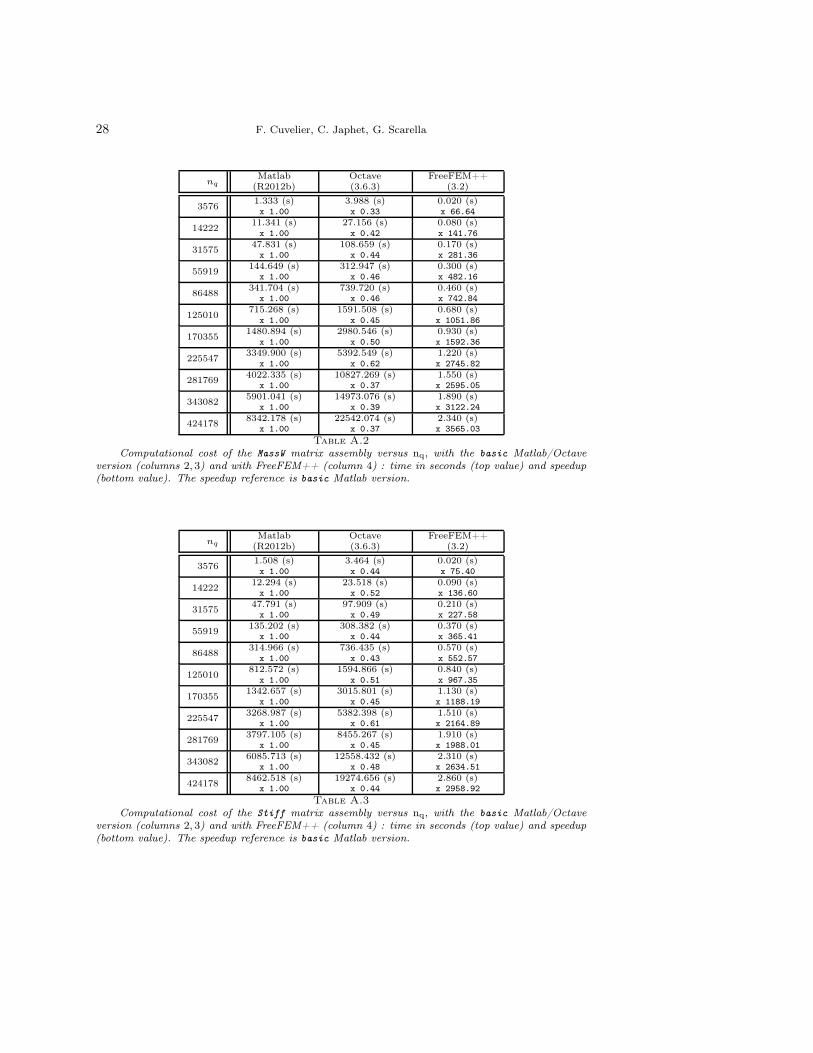
Computational cost of the MassW matrix assembly versus nq, with the basic Matlab/Octaveversion (columns 2, 3) and with FreeFEM++ (column 4) : time in seconds (top value) and speedup(bottom value). The speedup reference is basic Matlab version.
nqMatlab
(R2012b)Octave(3.6.3)
FreeFEM++(3.2)
35761.508 (s)x 1.00
3.464 (s)x 0.44
0.020 (s)x 75.40
1422212.294 (s)x 1.00
23.518 (s)x 0.52
0.090 (s)x 136.60
3157547.791 (s)x 1.00
97.909 (s)x 0.49
0.210 (s)x 227.58
55919135.202 (s)
x 1.00308.382 (s)
x 0.440.370 (s)x 365.41
86488314.966 (s)
x 1.00
736.435 (s)x 0.43
0.570 (s)x 552.57
125010812.572 (s)
x 1.00
1594.866 (s)x 0.51
0.840 (s)x 967.35
1703551342.657 (s)
x 1.00
3015.801 (s)x 0.45
1.130 (s)x 1188.19
2255473268.987 (s)
x 1.005382.398 (s)
x 0.611.510 (s)x 2164.89
2817693797.105 (s)
x 1.008455.267 (s)
x 0.451.910 (s)x 1988.01
3430826085.713 (s)
x 1.0012558.432 (s)
x 0.482.310 (s)x 2634.51
4241788462.518 (s)
x 1.0019274.656 (s)
x 0.442.860 (s)x 2958.92
Table A.3
Computational cost of the Stiff matrix assembly versus nq, with the basic Matlab/Octaveversion (columns 2, 3) and with FreeFEM++ (column 4) : time in seconds (top value) and speedup(bottom value). The speedup reference is basic Matlab version.

An efficient way to perform the assembly of finite element matrices in Matlab and Octave 29
A.2. OptV0 matrix assembly code vs FreeFEM++.
nqMatlab
(R2012b)Octave(3.6.3)
FreeFEM++(3.2)
35760.533 (s)x 1.00
1.988 (s)x 0.27
0.020 (s)x 26.67
142225.634 (s)x 1.00
24.027 (s)x 0.23
0.050 (s)x 112.69
3157529.042 (s)x 1.00
106.957 (s)x 0.27
0.120 (s)x 242.02
55919101.046 (s)
x 1.00
315.618 (s)x 0.32
0.210 (s)x 481.17
86488250.771 (s)
x 1.00
749.639 (s)x 0.33
0.340 (s)x 737.56
125010562.307 (s)
x 1.001582.636 (s)
x 0.360.480 (s)x 1171.47
1703551120.008 (s)
x 1.002895.512 (s)
x 0.390.670 (s)x 1671.65
2255472074.929 (s)
x 1.004884.057 (s)
x 0.420.880 (s)x 2357.87
2817693054.103 (s)
x 1.007827.873 (s)
x 0.391.130 (s)x 2702.75
3430824459.816 (s)
x 1.00
11318.536 (s)x 0.39
1.360 (s)x 3279.28
4241787638.798 (s)
x 1.00
17689.047 (s)x 0.43
1.700 (s)x 4493.41
Table A.4
Computational cost of the Mass matrix assembly versus nq, with the OptV0 Matlab/Octaveversion (columns 2, 3) and with FreeFEM++ (column 4) : time in seconds (top value) and speedup(bottom value). The speedup reference is OptV0 Matlab version.
nqMatlab
(R2012b)Octave(3.6.3)
FreeFEM++(3.2)
35760.638 (s)x 1.00
3.248 (s)x 0.20
0.020 (s)x 31.89
142226.447 (s)x 1.00
27.560 (s)x 0.23
0.080 (s)x 80.58
3157536.182 (s)x 1.00
114.969 (s)x 0.31
0.170 (s)x 212.83
55919125.339 (s)
x 1.00
320.114 (s)x 0.39
0.300 (s)x 417.80
86488339.268 (s)
x 1.00
771.449 (s)x 0.44
0.460 (s)x 737.54
125010584.245 (s)
x 1.001552.844 (s)
x 0.380.680 (s)x 859.18
1703551304.881 (s)
x 1.002915.124 (s)
x 0.450.930 (s)x 1403.10
2255472394.946 (s)
x 1.004934.726 (s)
x 0.491.220 (s)x 1963.07
2817693620.519 (s)
x 1.008230.834 (s)
x 0.441.550 (s)x 2335.82
3430825111.303 (s)
x 1.00
11788.945 (s)x 0.43
1.890 (s)x 2704.39
4241788352.331 (s)
x 1.00
18289.219 (s)x 0.46
2.340 (s)x 3569.37
Table A.5
Computational cost of the MassW matrix assembly versus nq, with the OptV0 Matlab/Octaveversion (columns 2, 3) and with FreeFEM++ (column 4) : time in seconds (top value) and speedup(bottom value). The speedup reference is OptV0 Matlab version.

30 F. Cuvelier, C. Japhet, G. Scarella
nqMatlab
(R2012b)Octave(3.6.3)
FreeFEM++(3.2)
35760.738 (s)x 1.00
2.187 (s)x 0.34
0.020 (s)x 36.88
142226.864 (s)x 1.00
23.037 (s)x 0.30
0.090 (s)x 76.26
3157532.143 (s)x 1.00
101.787 (s)x 0.32
0.210 (s)x 153.06
5591999.828 (s)x 1.00
306.232 (s)x 0.33
0.370 (s)x 269.81
86488259.689 (s)
x 1.00738.838 (s)
x 0.350.570 (s)x 455.59
125010737.888 (s)
x 1.00
1529.401 (s)x 0.48
0.840 (s)x 878.44
1703551166.721 (s)
x 1.00
2878.325 (s)x 0.41
1.130 (s)x 1032.50
2255472107.213 (s)
x 1.00
4871.663 (s)x 0.43
1.510 (s)x 1395.51
2817693485.933 (s)
x 1.007749.715 (s)
x 0.451.910 (s)x 1825.10
3430825703.957 (s)
x 1.0011464.992 (s)
x 0.502.310 (s)x 2469.25
4241788774.701 (s)
x 1.0017356.351 (s)
x 0.512.860 (s)x 3068.08
Table A.6
Computational cost of the Stiff matrix assembly versus nq, with the OptV0 Matlab/Octaveversion (columns 2, 3) and with FreeFEM++ (column 4) : time in seconds (top value) and speedup(bottom value). The speedup reference is OptV0 Matlab version.
A.3. OptV1 matrix assembly code vs FreeFEM++.
nqMatlab
(R2012b)Octave(3.6.3)
FreeFEM++(3.20)
142220.416 (s)x 1.00
2.022 (s)x 0.21
0.060 (s)x 6.93
559191.117 (s)x 1.00
8.090 (s)x 0.14
0.200 (s)x 5.58
1250102.522 (s)x 1.00
18.217 (s)x 0.14
0.490 (s)x 5.15
2255474.524 (s)x 1.00
32.927 (s)x 0.14
0.890 (s)x 5.08
3430827.105 (s)x 1.00
49.915 (s)x 0.14
1.370 (s)x 5.19
50670610.445 (s)x 1.00
73.487 (s)x 0.14
2.000 (s)x 5.22
68971614.629 (s)x 1.00
99.967 (s)x 0.15
2.740 (s)x 5.34
88552118.835 (s)x 1.00
128.529 (s)x 0.15
3.550 (s)x 5.31
112709023.736 (s)x 1.00
163.764 (s)x 0.14
4.550 (s)x 5.22
140112929.036 (s)x 1.00
202.758 (s)x 0.14
5.680 (s)x 5.11
167105235.407 (s)x 1.00
242.125 (s)x 0.15
6.810 (s)x 5.20
197860241.721 (s)x 1.00
286.568 (s)x 0.15
8.070 (s)x 5.17
Table A.7
Computational cost of the Mass matrix assembly versus nq, with the OptV1 Matlab/Octaveversion (columns 2, 3) and with FreeFEM++ (column 4) : time in seconds (top value) and speedup(bottom value). The speedup reference is OptV1 Matlab version.

An efficient way to perform the assembly of finite element matrices in Matlab and Octave 31
nqMatlab
(R2012b)Octave(3.6.3)
FreeFEM++(3.20)
142220.680 (s)x 1.00
4.633 (s)x 0.15
0.070 (s)x 9.71
559192.013 (s)x 1.00
18.491 (s)x 0.11
0.310 (s)x 6.49
1250104.555 (s)x 1.00
41.485 (s)x 0.11
0.680 (s)x 6.70
2255478.147 (s)x 1.00
74.632 (s)x 0.11
1.240 (s)x 6.57
34308212.462 (s)x 1.00
113.486 (s)x 0.11
1.900 (s)x 6.56
50670618.962 (s)x 1.00
167.979 (s)x 0.11
2.810 (s)x 6.75
68971625.640 (s)x 1.00
228.608 (s)x 0.11
3.870 (s)x 6.63
88552132.574 (s)x 1.00
292.502 (s)x 0.11
4.950 (s)x 6.58
112709042.581 (s)x 1.00
372.115 (s)x 0.11
6.340 (s)x 6.72
140112953.395 (s)x 1.00
467.396 (s)x 0.11
7.890 (s)x 6.77
167105261.703 (s)x 1.00
554.376 (s)x 0.11
9.480 (s)x 6.51
197860277.085 (s)x 1.00
656.220 (s)x 0.12
11.230 (s)x 6.86
Table A.8
Computational cost of the MassW matrix assembly versus nq, with the OptV1 Matlab/Octaveversion (columns 2, 3) and with FreeFEM++ (column 4) : time in seconds (top value) and speedup(bottom value). The speedup reference is OptV1 Matlab version.
nqMatlab
(R2012b)Octave(3.6.3)
FreeFEM++(3.20)
142221.490 (s)x 1.00
3.292 (s)x 0.45
0.090 (s)x 16.55
559194.846 (s)x 1.00
13.307 (s)x 0.36
0.360 (s)x 13.46
12501010.765 (s)x 1.00
30.296 (s)x 0.36
0.830 (s)x 12.97
22554719.206 (s)x 1.00
54.045 (s)x 0.36
1.500 (s)x 12.80
34308228.760 (s)x 1.00
81.988 (s)x 0.35
2.290 (s)x 12.56
50670642.309 (s)x 1.00
121.058 (s)x 0.35
3.390 (s)x 12.48
68971657.635 (s)x 1.00
164.955 (s)x 0.35
4.710 (s)x 12.24
88552173.819 (s)x 1.00
211.515 (s)x 0.35
5.960 (s)x 12.39
112709094.438 (s)x 1.00
269.490 (s)x 0.35
7.650 (s)x 12.34
1401129117.564 (s)
x 1.00335.906 (s)
x 0.359.490 (s)x 12.39
1671052142.829 (s)
x 1.00
397.392 (s)x 0.36
11.460 (s)x 12.46
1978602169.266 (s)
x 1.00
471.031 (s)x 0.36
13.470 (s)x 12.57
Table A.9
Computational cost of the Stiff matrix assembly versus nq, with the OptV1 Matlab/Octaveversion (columns 2, 3) and with FreeFEM++ (column 4) : time in seconds (top value) and speedup(bottom value). The speedup reference is OptV1 Matlab version.

32 F. Cuvelier, C. Japhet, G. Scarella
A.4. OptV2 matrix assembly code vs FreeFEM++.
nqOctave(3.6.3)
Matlab(R2012b)
FreeFEM++(3.20)
1250100.239 (s)x 1.00
0.422 (s)x 0.57
0.470 (s)x 0.51
2255470.422 (s)x 1.00
0.793 (s)x 0.53
0.880 (s)x 0.48
3430820.663 (s)x 1.00
1.210 (s)x 0.55
1.340 (s)x 0.49
5067060.990 (s)x 1.00
1.876 (s)x 0.53
2.000 (s)x 0.49
6897161.432 (s)x 1.00
2.619 (s)x 0.55
2.740 (s)x 0.52
8855211.843 (s)x 1.00
3.296 (s)x 0.56
3.510 (s)x 0.53
11270902.331 (s)x 1.00
4.304 (s)x 0.54
4.520 (s)x 0.52
14011292.945 (s)x 1.00
5.426 (s)x 0.54
5.580 (s)x 0.53
16710523.555 (s)x 1.00
6.480 (s)x 0.55
6.720 (s)x 0.53
19786024.175 (s)x 1.00
7.889 (s)x 0.53
7.940 (s)x 0.53
23495735.042 (s)x 1.00
9.270 (s)x 0.54
9.450 (s)x 0.53
27324485.906 (s)x 1.00
10.558 (s)x 0.56
11.000 (s)x 0.54
30856286.640 (s)x 1.00
12.121 (s)x 0.55
12.440 (s)x 0.53
Table A.10
Computational cost of the Mass matrix assembly versus nq, with the OptV2 Matlab/Octave codes(columns 2, 3) and with FreeFEM++ (column 4) : time in seconds (top value) and speedup (bottomvalue). The speedup reference is OptV2 Octave version.
nqOctave(3.6.3)
Matlab(R2012b)
FreeFEM++(3.20)
1250100.214 (s)x 1.00
0.409 (s)x 0.52
0.680 (s)x 0.31
2255470.405 (s)x 1.00
0.776 (s)x 0.52
1.210 (s)x 0.33
3430820.636 (s)x 1.00
1.229 (s)x 0.52
1.880 (s)x 0.34
5067060.941 (s)x 1.00
1.934 (s)x 0.49
2.770 (s)x 0.34
6897161.307 (s)x 1.00
2.714 (s)x 0.48
4.320 (s)x 0.30
8855211.791 (s)x 1.00
3.393 (s)x 0.53
4.880 (s)x 0.37
11270902.320 (s)x 1.00
4.414 (s)x 0.53
6.260 (s)x 0.37
14011292.951 (s)x 1.00
5.662 (s)x 0.52
7.750 (s)x 0.38
16710523.521 (s)x 1.00
6.692 (s)x 0.53
9.290 (s)x 0.38
19786024.201 (s)x 1.00
8.169 (s)x 0.51
11.000 (s)x 0.38
23495735.456 (s)x 1.00
9.564 (s)x 0.57
13.080 (s)x 0.42
27324486.178 (s)x 1.00
10.897 (s)x 0.57
15.220 (s)x 0.41
30856286.854 (s)x 1.00
12.535 (s)x 0.55
17.190 (s)x 0.40
Table A.11
Computational cost of the MassW matrix assembly versus nq, with the OptV2 Matlab/Octavecodes (columns 2, 3) and with FreeFEM++ (column 4) : time in seconds (top value) and speedup(bottom value). The speedup reference is OptV2 Octave version.

An efficient way to perform the assembly of finite element matrices in Matlab and Octave 33
nqOctave(3.6.3)
Matlab(R2012b)
FreeFEM++(3.20)
1250100.227 (s)x 1.00
0.453 (s)x 0.50
0.800 (s)x 0.28
2255470.419 (s)x 1.00
0.833 (s)x 0.50
1.480 (s)x 0.28
3430820.653 (s)x 1.00
1.323 (s)x 0.49
2.260 (s)x 0.29
5067060.981 (s)x 1.00
1.999 (s)x 0.49
3.350 (s)x 0.29
6897161.354 (s)x 1.00
2.830 (s)x 0.48
4.830 (s)x 0.28
8855211.889 (s)x 1.00
3.525 (s)x 0.54
5.910 (s)x 0.32
11270902.385 (s)x 1.00
4.612 (s)x 0.52
7.560 (s)x 0.32
14011293.021 (s)x 1.00
5.810 (s)x 0.52
9.350 (s)x 0.32
16710523.613 (s)x 1.00
6.899 (s)x 0.52
11.230 (s)x 0.32
19786024.294 (s)x 1.00
8.504 (s)x 0.50
13.280 (s)x 0.32
23495735.205 (s)x 1.00
9.886 (s)x 0.53
16.640 (s)x 0.31
27324486.430 (s)x 1.00
11.269 (s)x 0.57
19.370 (s)x 0.33
30856287.322 (s)x 1.00
13.049 (s)x 0.56
20.800 (s)x 0.35
Table A.12
Computational cost of the Stiff matrix assembly versus nq, with the OptV2 Matlab/Octavecodes (columns 2, 3) and with FreeFEM++ (column 4) : time in seconds (top value) and speedup(bottom value). The speedup reference is OptV2 Octave version.
Appendix B. Matrix assembly codes.
B.1. Element matrices.
Listing 16
ElemMassMatP1.m
1 function AElem=ElemMassMatP1 ( area )2 AElem=(area /12)∗ [2 1 1 ; 1 2 1 ; 1 1 2 ] ;
Listing 17
ElemMassWMatP1.m
1 function AElem=ElemMassWMatP1( area ,w)2 AElem=(area /30)∗ . . .3 [ 3∗w(1)+w(2)+w(3 ) , w(1)+w(2)+w(3)/2 , w(1)+w(2)/2+w( 3 ) ; . . .4 w(1)+w(2)+w(3)/2 , w(1)+3∗w(2)+w(3 ) , w(1)/2+w(2)+w( 3 ) ; . . .5 w(1)+w(2)/2+w(3 ) , w(1)/2+w(2)+w(3 ) , w(1)+w(2)+3∗w( 3 ) ] ;
Listing 18
ElemStiffMatP1.m
1 function AElem=ElemStiffMatP1 (q1 , q2 , q3 , area )2 M=[q2´q3 , q3´q1 , q1´q2 ] ;3 AElem=(1/(4∗ area ) )∗M’∗M;

34 F. Cuvelier, C. Japhet, G. Scarella
B.2. Classical matrix assembly code.
Listing 19
MassAssemblingP1base.m
1 function M=MassAssemblingP1base (nq , nme ,me, areas )2 M=sparse (nq , nq ) ;3 for k=1:nme4 E=ElemMassMatP1 ( areas (k ) ) ;5 for i l =1:36 i=me( i l , k ) ;7 for j l =1:38 j=me( j l , k ) ;9 M( i , j )=M( i , j )+E( i l , j l ) ;
10 end
11 end
12 end
Listing 20
MassWAssemblingP1base.m
1 function M=MassWAssemblingP1base(nq , nme ,me, areas ,Tw)2 M=sparse (nq , nq ) ;3 for k=1:nme4 for i l =1:35 i=me( i l , k ) ;6 Twloc ( i l )=Tw( i ) ;7 end
8 E=ElemMassWMatP1( areas ( k ) , Twloc ) ;9 for i l =1:3
10 i=me( i l , k ) ;11 for j l =1:312 j=me( j l , k ) ;13 M( i , j )=M( i , j )+E( i l , j l ) ;14 end
15 end
16 end
Listing 21
StiffAssemblingP1base.m
1 function R=Sti f fAssembl ingP1base (nq , nme , q ,me, ar eas )2 R=sparse (nq , nq ) ;3 for k=1:nme4 E=ElemStiffMatP1 (q ( : ,me(1 , k ) ) , q ( : ,me(2 , k ) ) , q ( : ,me(3 , k ) ) , a r eas ( k ) ) ;5 for i l =1:36 i=me( i l , k ) ;7 for j l =1:38 j=me( j l , k ) ;9 R( i , j )=R( i , j )+E( i l , j l ) ;
10 end
11 end
12 end

An efficient way to perform the assembly of finite element matrices in Matlab and Octave 35
B.3. Optimized matrix assembly codes - Version 0.
Listing 22
MassAssemblingP1OptV0.m
1 function M=MassAssemblingP1OptV0 (nq , nme ,me, areas )2 M=sparse (nq , nq ) ;3 for k=1:nme4 I=me ( : , k ) ;5 M( I , I )=M( I , I )+ElemMassMatP1 ( areas ( k ) ) ;6 end
Listing 23
MassWAssemblingP1OptV0.m
1 function M=MassWAssemblingP1OptV0(nq , nme ,me, areas ,Tw)2 M=sparse (nq , nq ) ;3 for k=1:nme4 I=me ( : , k ) ;5 M( I , I )=M( I , I )+ElemMassWMatP1( areas ( k ) ,Tw(me( : , k ) ) ) ;6 end
Listing 24
StiffAssemblingP1OptV0.m
1 function R=StiffAssemblingP1OptV0 (nq , nme , q ,me, ar eas )2 R=sparse (nq , nq ) ;3 for k=1:nme4 I=me ( : , k ) ;5 Me=ElemStiffMatP1 (q ( : ,me(1 , k ) ) , q ( : ,me(2 , k ) ) , q ( : ,me(3 , k ) ) , a r eas ( k ) ) ;6 R( I , I )=R( I , I )+Me;7 end
B.4. Optimized matrix assembly codes - Version 1.
Listing 25
MassAssemblingP1OptV1.m
1 function M=MassAssemblingP1OptV1 (nq , nme ,me, areas )2 Ig=zeros (9∗nme , 1 ) ; Jg=zeros (9∗nme , 1 ) ;Kg=zeros (9∗nme , 1 ) ;3
4 i i =[1 2 3 1 2 3 1 2 3 ] ;5 j j =[1 1 1 2 2 2 3 3 3 ] ;6 kk=1:9 ;7 for k=1:nme8 E=ElemMassMatP1 ( areas (k ) ) ;9 Ig ( kk)=me( i i , k ) ;
10 Jg ( kk)=me( j j , k ) ;11 Kg( kk)=E ( : ) ;12 kk=kk+9;13 end
14 M=sparse ( Ig , Jg ,Kg, nq , nq ) ;
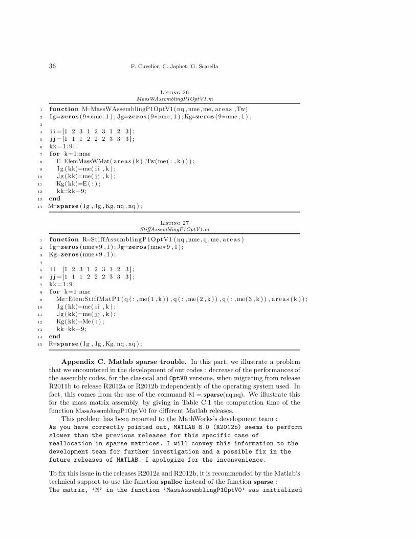
36 F. Cuvelier, C. Japhet, G. Scarella
Listing 26
MassWAssemblingP1OptV1.m
1 function M=MassWAssemblingP1OptV1(nq , nme ,me, areas ,Tw)2 Ig=zeros (9∗nme , 1 ) ; Jg=zeros (9∗nme , 1 ) ;Kg=zeros (9∗nme , 1 ) ;3
4 i i =[1 2 3 1 2 3 1 2 3 ] ;5 j j =[1 1 1 2 2 2 3 3 3 ] ;6 kk=1:9 ;7 for k=1:nme8 E=ElemMassWMat( areas (k ) ,Tw(me( : , k ) ) ) ;9 Ig ( kk)=me( i i , k ) ;
10 Jg ( kk)=me( j j , k ) ;11 Kg( kk)=E ( : ) ;12 kk=kk+9;13 end
14 M=sparse ( Ig , Jg ,Kg, nq , nq ) ;
Listing 27
StiffAssemblingP1OptV1.m
1 function R=StiffAssemblingP1OptV1 (nq , nme , q ,me, ar eas )2 Ig=zeros (nme∗9 , 1 ) ; Jg=zeros (nme∗9 , 1 ) ;3 Kg=zeros (nme∗9 , 1 ) ;4
5 i i =[1 2 3 1 2 3 1 2 3 ] ;6 j j =[1 1 1 2 2 2 3 3 3 ] ;7 kk=1:9 ;8 for k=1:nme9 Me=ElemStiffMatP1 (q ( : ,me(1 , k ) ) , q ( : ,me(2 , k ) ) , q ( : ,me(3 , k ) ) , a r eas ( k ) ) ;
10 Ig ( kk)=me( i i , k ) ;11 Jg ( kk)=me( j j , k ) ;12 Kg( kk)=Me ( : ) ;13 kk=kk+9;14 end
15 R=sparse ( Ig , Jg ,Kg, nq , nq ) ;
Appendix C. Matlab sparse trouble. In this part, we illustrate a problemthat we encountered in the development of our codes : decrease of the performances ofthe assembly codes, for the classical and OptV0 versions, when migrating from releaseR2011b to release R2012a or R2012b independently of the operating system used. Infact, this comes from the use of the command M = sparse(nq,nq). We illustrate thisfor the mass matrix assembly, by giving in Table C.1 the computation time of thefunction MassAssemblingP1OptV0 for different Matlab releases.
This problem has been reported to the MathWorks’s development team :As you have correctly pointed out, MATLAB 8.0 (R2012b) seems to perform
slower than the previous releases for this specific case of
reallocation in sparse matrices. I will convey this information to the
development team for further investigation and a possible fix in the
future releases of MATLAB. I apologize for the inconvenience.
To fix this issue in the releases R2012a and R2012b, it is recommended by the Matlab’stechnical support to use the function spalloc instead of the function sparse :The matrix, ’M’ in the function ’MassAssemblingP1OptV0’ was initialized

An efficient way to perform the assembly of finite element matrices in Matlab and Octave 37
using SPALLOC instead of the SPARSE command since the maximum number of
non-zeros in M are already known.
Previously existing line of code:
M = sparse(nq,nq);
Modified line of code:
M = spalloc(nq, nq, 9*nme);
Sparse dim R2012b R2012a R2011b R2011a
16000.167 (s)pˆ1.00q
0.155 (s)pˆ1.07q
0.139 (s)pˆ1.20q
0.116 (s)pˆ1.44q
36000.557 (s)pˆ1.00q
0.510 (s)pˆ1.09q
0.461 (s)pˆ1.21q
0.355 (s)pˆ1.57q
64001.406 (s)pˆ1.00q
1.278 (s)pˆ1.10q
1.150 (s)pˆ1.22q
0.843 (s)pˆ1.67q
100004.034 (s)pˆ1.00q
2.761 (s)pˆ1.46q
1.995 (s)pˆ2.02q
1.767 (s)pˆ2.28q
144008.545 (s)pˆ1.00q
6.625 (s)pˆ1.29q
3.734 (s)pˆ2.29q
3.295 (s)pˆ2.59q
1960016.643 (s)
pˆ1.00q13.586 (s)
pˆ1.22q6.908 (s)pˆ2.41q
6.935 (s)pˆ2.40q
2560029.489 (s)
pˆ1.00q27.815 (s)
pˆ1.06q12.367 (s)
pˆ2.38q11.175 (s)
pˆ2.64q
3240047.478 (s)
pˆ1.00q47.037 (s)
pˆ1.01q18.457 (s)
pˆ2.57q16.825 (s)
pˆ2.82q
4000073.662 (s)
pˆ1.00q74.188 (s)
pˆ0.99q27.753 (s)
pˆ2.65q25.012 (s)
pˆ2.95q
Table C.1
MassAssemblingP1OptV0 for different Matlab releases : computation times and speedupREFERENCES
[1] C. Bernardi, Y. Maday, and A. Patera, A new nonconforming approach to domain de-composition: the mortar element method, in Nonlinear Partial Differential Equations andtheir Applications, H. Brezis and J.L. Lions, eds., 1989.
[2] L. Chen, Programming of Finite Element Methods in Matlab, Preprint, University of CaliforniaIrvine, http://math.uci.edu/~chenlong/226/Ch3FEMCode.pdf , 2011.
[3] L. Chen, iFEM, a Matlab software package, University of California Irvine,http://math.uci.edu/~chenlong/programming.html , 2013.
[4] P. G. Ciarlet, The finite element method for elliptic problems, SIAM, Philadelphia, 2002.[5] F. Cuvelier, Méthodes des éléments finis. De la théorie
à la programmation, Lecture Notes, Université Paris 13,http://www.math.univ-paris13.fr/~cuvelier/docs/poly/polyFEM2D.pdf , 2008.
[6] F. Cuvelier, C. Japhet, and G. Scarella, OptFEM2DP1, a MATLAB/Octave softwarepackage codes, Université Paris 13, http://www.math.univ-paris13.fr/~cuvelier , 2012.
[7] F. Cuvelier, C. Japhet, and G. Scarella, An efficient way to perform the assembly offinite element matrices in Matlab and Octave: the Pk finite element case, in preparation.
[8] T. A. Davis, Direct Methods for Sparse Linear Systems, SIAM, 2006.[9] T. A. Davis, SuiteSparse packages, release 4.0.12, University of Florida,
http://www.cise.ufl.edu/research/sparse/SuiteSparse , 2012.[10] G. Dhatt, E. Lefrançois, and G. Touzot, Finite Element Method, Wiley, 2012.[11] GNU Octave, http://www.gnu.org/software/octave , 2012.[12] A. Hannukainen, and M. Juntunen, Implementing the Finite Ele-
ment Assembly in Interpreted Languages, Preprint, Aalto University,http://users.tkk.fi/~mojuntun/preprints/matvecSISC.pdf, 2012.
[13] F. Hecht, FreeFEM++, http://www.freefem.org/ff++/index.htm , 2012.[14] C. Johnson, Numerical Solution of Partial Differential Equations by the Finite Element
Method, Dover Publications, Inc, 2009.[15] B. Lucquin, and O. Pironneau, Introduction to Scientific Computing, John Wiley & Sons
Ltd, 1998.[16] MATLAB, http://www.mathworks.com , 2012.[17] T. Rahman, and J. Valdman, Fast MATLAB assembly of FEM matrices in 2D and 3D:
Nodal elements, Appl. Math. Comput., 219(13) (2013), pp. 7151–7158.

RESEARCH CENTREPARIS – ROCQUENCOURT
Domaine de Voluceau, - Rocquencourt
B.P. 105 - 78153 Le Chesnay Cedex
PublisherInriaDomaine de Voluceau - RocquencourtBP 105 - 78153 Le Chesnay Cedexinria.fr
ISSN 0249-6399

104
105
106
107
10−2
10−1
100
101
102
103
104
nq
time
(s)
MatlabOctaveFreeFEM++O(n
q)
O(nq2)