an economic analysis of the circular economy - … · an economic analysis of the circular economy...
TRANSCRIPT
1
An Economic Analysis of The Circular Economy
Sugandha D Tuladhar1, Mei Yuan2, and W. David Montgomery3
Paper prepared for the 19th Annual Conference on Global Economic Analysis “Analytical Foundations for Cooperation in a Multipolar World,”
NERA Economic Consulting
Washington, DC, June 15-17, 2016.
Abstract In this paper we develop a global computable general equilibrium (CGE) model to evaluate the effects of illustrative circular economy scenarios for Denmark and the European Union using the GTAP 8 dataset. The goal of a circular economy is to minimize the use of virgin resources and the generation of residuals not re-used in production. We simulate four circularity scenarios – two Denmark specific circularity scenarios and two scenarios that affect the European Union. The modeling results show that Denmark’s gross domestic product (GDP) could increase by 0.8% to 1.4% relative to the baseline by 2035. Under similar circular economy assumptions, European Union’s GDP could increase by 1.4% to 2.7% by 2035 relative to the baseline. Our sectoral modeling results show that the construction sector in Denmark contributes more than half of the GDP growth. The rest of the GDP growth comes from other sectors therefore playing an important role in placing the economy on a sustainable growth path. The scenarios assume that there are no upfront economic costs and opportunity costs of achieving the efficiency improvements that define the circular economy. Keywords: Circular economy, zero waste, recycling, sustainability, energy efficiency, macroeconomic impact
1 Vice President, NERA Economic Consulting, 1255 23rd Street, NW, Suite 600, Washington, DC 20037 Corresponding author: [email protected] Paper prepared for the 19th Annual Conference on Global Economic Analysis “Analytical Foundations for Cooperation in a Multipolar World,” Washington, DC, June 15-17, 2016. 2 MIT Joint Program on The Science and Policy of Global Change 3 Affiliated Consultant, NERA Economic Consulting, Washington DC The authors would like to thank an anonymous reviewer for providing helpful comments and suggestions. The views expressed in this paper are those of the authors and the authors take full responsibility for all errors and omissions.
2
Introduction
Global population has more than doubled in the last fifty years (3.3 billion in 1965 to about 7.3
billion in 2015 (World Bank)). During the same period global gross domestic production (GDP)
increased by more than fourfold. Looking into the future, world population could grow by an
additional 2 billion people by 2050 and global GDP could grow to more than three times its
current level. As the global economy grows and economies get more affluent, consumption of
material and waste from usage will also increase. According to one estimate, during the past
century waste from consumption and production increased by more than tenfold and could
double again over the next decade (Hoornweg 2013).
Concerns that global resources and capacity to absorb waste are depleting lead to pressure for
more efficient use of scarce resources either by consuming less, sharing resources, effectively
minimizing waste or transforming waste into useful materials. If the value of non-marketed
goods such as waste and product residuals could be increased by transforming them into forms
that can be used as substitutes for produced inputs or virgin materials, it might be possible to
move toward a circular economy with lesser generation of waste. If the cost of using residuals as
inputs to production could be brought below the cost of virgin resources, the result could be both
improved economic performance and reduced residual generation.
In this paper we develop a global computable general equilibrium (CGE) model to evaluate the
effects of illustrative circular economy scenarios for Denmark and European Union (EU). The
paper shows that under a simple formulation to represent a circular economy, economic growth
could be increased and resources used in a more sustainable way. The remainder of the paper is
organized as follows. Section 2 provides a brief description of how the circular economy can be
represented. Section 3 presents our approach to represent circularity within a CGE model.
Section 4 describes the scenarios. Section 5 discusses model results. We conclude in section 6.
1. Representing the circular economy in a CGE framework
Proposals for a circular economy purport to maximize the value of products, materials and
resources as long as possible, minimize waste generation, and develop a sustainable, efficient,
and competitive economy (European Commission 2015). The first requirement for a full

3
representation of circularity in a CGE framework is to incorporate a table of material flows that
is parallel to the input-output table of flows of goods and services (see Ayres, D’Arge and
Kneese (1969) and Noll and Trijonis (1971)). The CGE framework can be extended to
incorporate concepts of circularity based on the material flows. In this framework, we can
introduce a circular activity which involves refurbishing, remanufacturing, recycling or
regenerating what would otherwise be residuals. This activity takes waste and residues as inputs.
The outputs of this process can then be substituted for virgin materials or other factors of
production, for intermediate goods, and for investment or consumption as components of final
demand.
Extending a general equilibrium model to account for the full circular flow of all materials is
conceptually straightforward, but data requirements and computational complexities are so large
that there are only a few examples of data-based models of this type (See Kang 2006).
In absence of such material flows for the economy under study, we can think of circularity as the
allocative efficiency improvement achieved by a new technology on the output side that allows
wastes to be marketed and a new technology on the input side that provides cost savings due to
recycling activities. Efficiency improvements are readily incorporated into production functions
used in CGE models. Production functions typically contain parameters that govern the overall
efficiency of production or the productivity of specific inputs. Increasing the parameter for
overall productivity implies that the same amount of output can be produced with a
proportionally smaller utilization of every input. The parameters for each individual input (or
virgin material or residual) can be adjusted to represent technology changes that make it possible
to produce the same amount of output with less of that specific input, virgin material or residual.
Consumer behavior can be represented with essentially similar mathematical constructions to
those used to represent residuals generation, substitution and efficiency improvements in
production.
This approach involves an offline calculation of the output augmentation and input savings to
reparametrize the production function. The modified production function represents the
technology that embodies circular activities. Comparing with the baseline, we can find out the
contribution of circular activities by sector or as an aggregate to the economy.
4
It is useful to think of circularity as being based on specific kinds of technology improvements to
avoid creating the impression that the move to a more circular economy would be cost free. If
such technologies were available today, it would be necessary for us to assume that they are
more costly than less “circular” technologies in order to create a baseline in which they are not
adopted. In such a case, a model of the competitive market would show that policies mandating
the use of such technologies would produce net economic costs unless some specific market
imperfections that prevented their use were introduced into the baseline as well.
2. The Global NewERA Model
The Global NewERA model is a forward-looking, dynamic computable general equilibrium (CGE)
model of the world economy. It is built on the GTAP dataset and based on the theoretical
concept of an equilibrium in which macro-level outcomes are driven by the decisions of self-
interested consumers and producers. The basic structure of CGE models, such as NewERA, is
built around a circular flow of goods and payments between households, firms, and the
government.
The Global NewERA model is used extensively in the energy and environmental policy analysis,
including studies of the effects of carbon restrictions on trade and economic welfare in different
regions of the world. The model includes a disaggregated representation of industries, based on
the GTAP 8 dataset, so that differences in energy intensities across countries and differences in
the composition of industry can be taken into account. It can represent a wide variety of
international emissions trading regimes, define trading blocs composed of any grouping of
regions, and place any set of constraints on both purchases and sales of emissions permits. The
model computes changes in welfare (calculated as the infinite horizon equivalent variation),
national income and its components, terms of trade, output, imports and exports by commodity,
carbon emissions, and capital flows. It is fully dynamic, with saving and investment decisions
based on full intertemporal optimization. The model is written in GAMS/MPSGE which is a
non-algebraic computer language for the formulation of applied general equilibrium models
(Rutherford 1998).
Conceptually, the NewERA model computes a global equilibrium in which supply and demand
are equated simultaneously in all markets. The model assumes full employment and there is no
5
money. There is a representative agent in each region, and goods are indexed by region and time.
The budget constraint in the model implies that there can be no change in any region’s net
foreign indebtedness over the time horizon of the model. Even though there is no money in the
model, changes in the prices of internationally traded goods produce changes in the real terms of
trade between regions. All markets clear simultaneously, so that agents correctly anticipate all
future changes in terms of trade and take them into account in saving and investment decisions.
A technical description is shown in Appendix A.
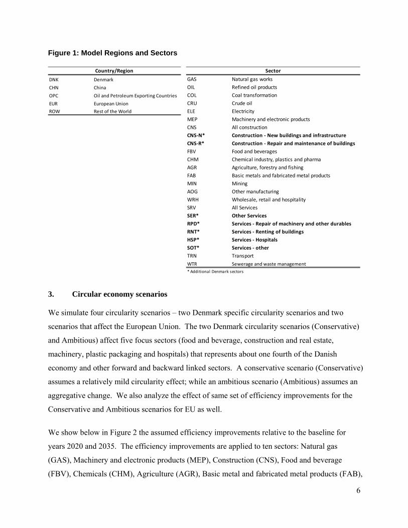
For this study, we aggregate the world into five regions – Denmark (DNK), China (CHN), Oil
exporting countries (OPC), European Union (EUR) excluding Denmark, and Rest of the world
(ROW). Each region includes 5 energy and 12 non-energy sectors. For Denmark, we
disaggregate the Construction and the Services sectors, to capture sectoral circularity effects in
greater detail for Denmark. The model includes 22 production sectors for Denmark. The details
of the model regions and sectors are shown in Figure 1 below. The NewERA model is based on
the GTAP 8 dataset. We construct a global economic dataset consistent with 2011 economic
conditions. We first estimate GDP growth rates from 2007 to 2011 for China, Oil exporting
countries, European Union, and Rest of the world. We then apply these growth rates to estimate
2011 economic flows (or 2011 Input Output table). We replace Denmark’s 2007 GTAP8 flows
by Denmark’s 2011 Input Output flows. We then rebalance this adjusted dataset to create a
globally balanced 2011 dataset.
6
Figure 1: Model Regions and Sectors
3. Circular economy scenarios
We simulate four circularity scenarios – two Denmark specific circularity scenarios and two
scenarios that affect the European Union. The two Denmark circularity scenarios (Conservative)
and Ambitious) affect five focus sectors (food and beverage, construction and real estate,
machinery, plastic packaging and hospitals) that represents about one fourth of the Danish
economy and other forward and backward linked sectors. A conservative scenario (Conservative)
assumes a relatively mild circularity effect; while an ambitious scenario (Ambitious) assumes an
aggregative change. We also analyze the effect of same set of efficiency improvements for the
Conservative and Ambitious scenarios for EU as well.
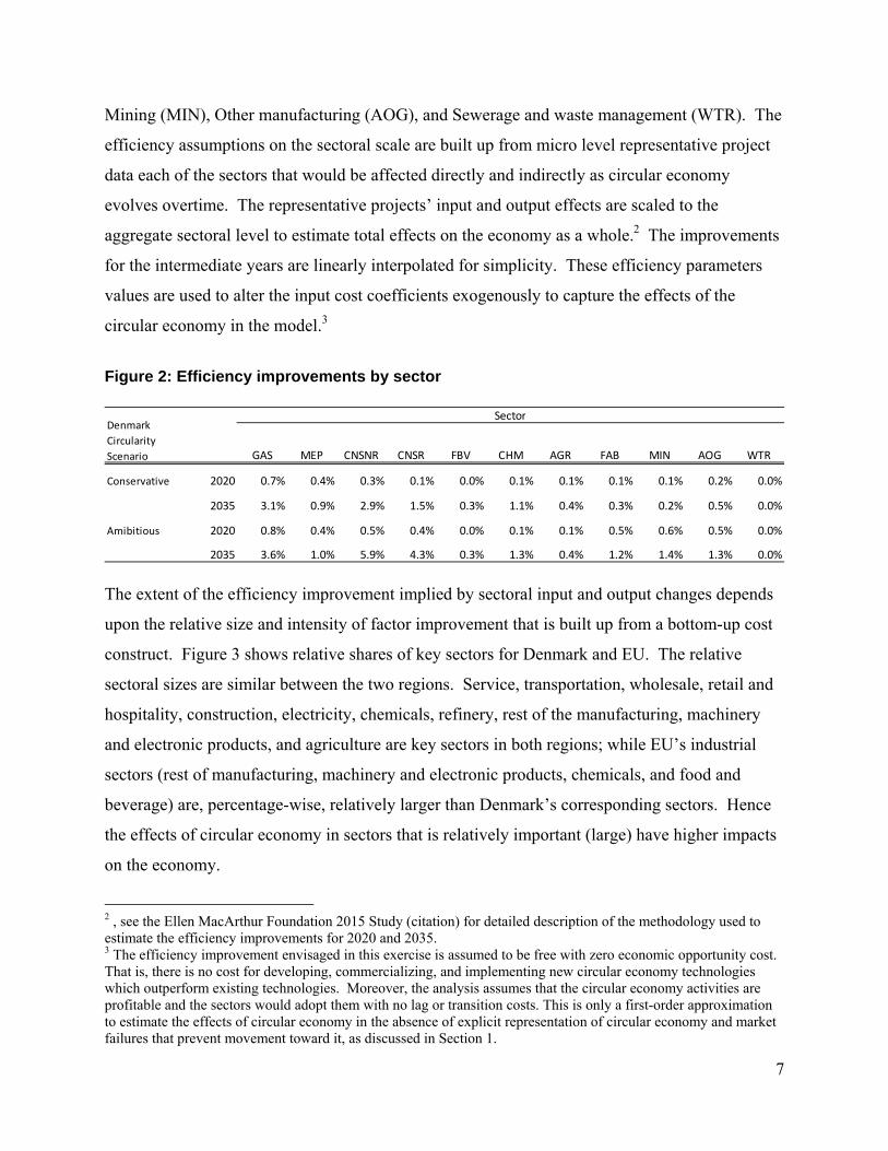
We show below in Figure 2 the assumed efficiency improvements relative to the baseline for
years 2020 and 2035. The efficiency improvements are applied to ten sectors: Natural gas
(GAS), Machinery and electronic products (MEP), Construction (CNS), Food and beverage
(FBV), Chemicals (CHM), Agriculture (AGR), Basic metal and fabricated metal products (FAB),
DNK Denmark GAS Natural gas works
CHN China OIL Refined oil products
OPC Oil and Petroleum Exporting Countries COL Coal transformation
EUR European Union CRU Crude oil
ROW Rest of the World ELE Electricity
MEP Machinery and electronic products
CNS All construction
CNS‐N* Construction ‐ New buildings and infrastructure
CNS‐R* Construction ‐ Repair and maintenance of buildings
FBV Food and beverages
CHM Chemical industry, plastics and pharma
AGR Agriculture, forestry and fishing
FAB Basic metals and fabricated metal products
MIN Mining
AOG Other manufacturing
WRH Wholesale, retail and hospitality
SRV All Services
SER* Other Services
RPD* Services ‐ Repair of machinery and other durables
RNT* Services ‐ Renting of buildings
HSP* Services ‐ Hospitals
SOT* Services ‐ other
TRN Transport
WTR Sewerage and waste management
* Additional Denmark sectors
SectorCountry/Region
7
Mining (MIN), Other manufacturing (AOG), and Sewerage and waste management (WTR). The
efficiency assumptions on the sectoral scale are built up from micro level representative project
data each of the sectors that would be affected directly and indirectly as circular economy
evolves overtime. The representative projects’ input and output effects are scaled to the
aggregate sectoral level to estimate total effects on the economy as a whole.2 The improvements
for the intermediate years are linearly interpolated for simplicity. These efficiency parameters
values are used to alter the input cost coefficients exogenously to capture the effects of the
circular economy in the model.3
Figure 2: Efficiency improvements by sector
The extent of the efficiency improvement implied by sectoral input and output changes depends
upon the relative size and intensity of factor improvement that is built up from a bottom-up cost
construct. Figure 3 shows relative shares of key sectors for Denmark and EU. The relative
sectoral sizes are similar between the two regions. Service, transportation, wholesale, retail and
hospitality, construction, electricity, chemicals, refinery, rest of the manufacturing, machinery
and electronic products, and agriculture are key sectors in both regions; while EU’s industrial
sectors (rest of manufacturing, machinery and electronic products, chemicals, and food and
beverage) are, percentage-wise, relatively larger than Denmark’s corresponding sectors. Hence
the effects of circular economy in sectors that is relatively important (large) have higher impacts
on the economy.
2 , see the Ellen MacArthur Foundation 2015 Study (citation) for detailed description of the methodology used to estimate the efficiency improvements for 2020 and 2035. 3 The efficiency improvement envisaged in this exercise is assumed to be free with zero economic opportunity cost. That is, there is no cost for developing, commercializing, and implementing new circular economy technologies which outperform existing technologies. Moreover, the analysis assumes that the circular economy activities are profitable and the sectors would adopt them with no lag or transition costs. This is only a first-order approximation to estimate the effects of circular economy in the absence of explicit representation of circular economy and market failures that prevent movement toward it, as discussed in Section 1.
GAS MEP CNSNR CNSR FBV CHM AGR FAB MIN AOG WTR
Conservative 2020 0.7% 0.4% 0.3% 0.1% 0.0% 0.1% 0.1% 0.1% 0.1% 0.2% 0.0%
2035 3.1% 0.9% 2.9% 1.5% 0.3% 1.1% 0.4% 0.3% 0.2% 0.5% 0.0%
Amibitious 2020 0.8% 0.4% 0.5% 0.4% 0.0% 0.1% 0.1% 0.5% 0.6% 0.5% 0.0%
2035 3.6% 1.0% 5.9% 4.3% 0.3% 1.3% 0.4% 1.2% 1.4% 1.3% 0.0%
SectorDenmark
Circularity
Scenario

8
Figure 3: Share of sectoral output relative to the total industrial output for Denmark and EU (%)
4. Results
The efficiency improvements by which we quantify sector-specific impacts of new circular
technologies lead to net value creation through economizing on inputs and producing more
valuable outputs or lower cheaper outputs. All sectors of the economy experience savings or
costs from using lower cost parts and components in the manufacturing process, materials, labor,
services, energy, and capital. In addition, output revenue effects due to incremental
profitability/sales are also estimated. The shift in technologies leads to greater output per unit of
input in the specified sectors of the Danish economy and therefore increased sectoral profitability.
These changes capture two primary effects of the circular economy: (i) reduce economy-wide
inputs or resource intensity to reflect waste recycling; and (ii) change production and
consumption technologies by changing the goods intensity or the mixture of intermediate
demand for goods and services to produce a commodity.
In all scenarios circularity leads to higher levels of economic activity. Higher efficiency,
particularly in the focus sectors, means that goods and services can be produced at lower costs
hence making these goods more competitive.
4.1 Circular economy leads to lower output prices for key economic sectors
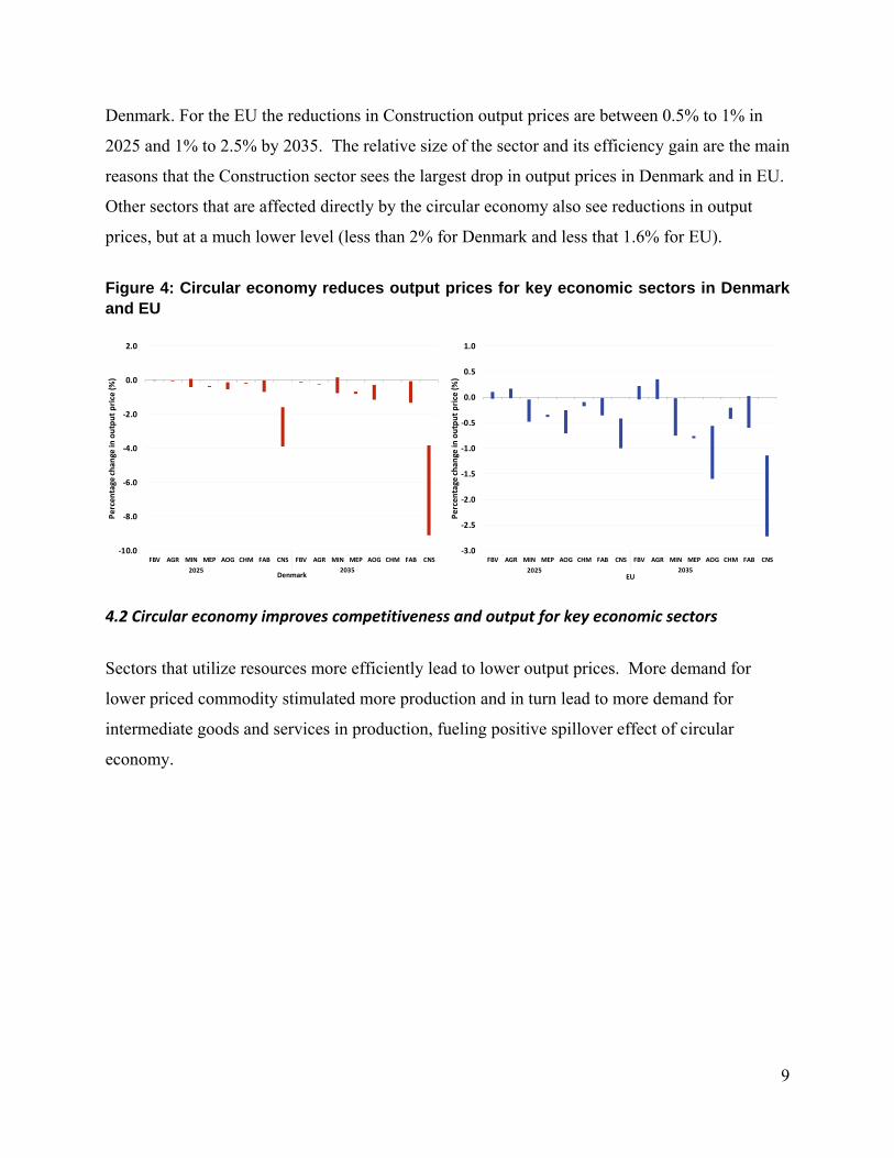
Figure 4 shows impacts on some key industrial sector output prices in Denmark and EU. Output
prices of the Construction sector decrease by 2% to 4% in 2025 and 4% to 9% by 2035 for
0.0
5.0
10.0
15.0
20.0
25.0
30.0
35.0
SER TRNWRH CNS ELE FBV CHM OIL AOG MEP AGRWTR CRU FAB GAS MIN COL
Share of sectoral output
relative to total sectoral output (%
)
Denmark
0.0
5.0
10.0
15.0
20.0
25.0
30.0
SER AOGWRH CNS TRN CHMMEP FBV FAB OIL ELE AGR GAS CRU MIN WTR COL
Share of sectoral output
relative to total sectoral output (%
)
EU
9
Denmark. For the EU the reductions in Construction output prices are between 0.5% to 1% in
2025 and 1% to 2.5% by 2035. The relative size of the sector and its efficiency gain are the main
reasons that the Construction sector sees the largest drop in output prices in Denmark and in EU.
Other sectors that are affected directly by the circular economy also see reductions in output
prices, but at a much lower level (less than 2% for Denmark and less that 1.6% for EU).
Figure 4: Circular economy reduces output prices for key economic sectors in Denmark and EU
4.2 Circular economy improves competitiveness and output for key economic sectors
Sectors that utilize resources more efficiently lead to lower output prices. More demand for
lower priced commodity stimulated more production and in turn lead to more demand for
intermediate goods and services in production, fueling positive spillover effect of circular
economy.
‐10.0
‐8.0
‐6.0
‐4.0
‐2.0
0.0
2.0
FBV AGR MIN MEP AOG CHM FAB CNS FBV AGR MIN MEP AOG CHM FAB CNS
Percentage change in
output price (%)
2025 2035Denmark
‐3.0
‐2.5
‐2.0
‐1.5
‐1.0
‐0.5
0.0
0.5
1.0
FBV AGR MIN MEP AOG CHM FAB CNS FBV AGR MIN MEP AOG CHM FAB CNS
Percentage change in
output price (%)
2025 2035EU
10
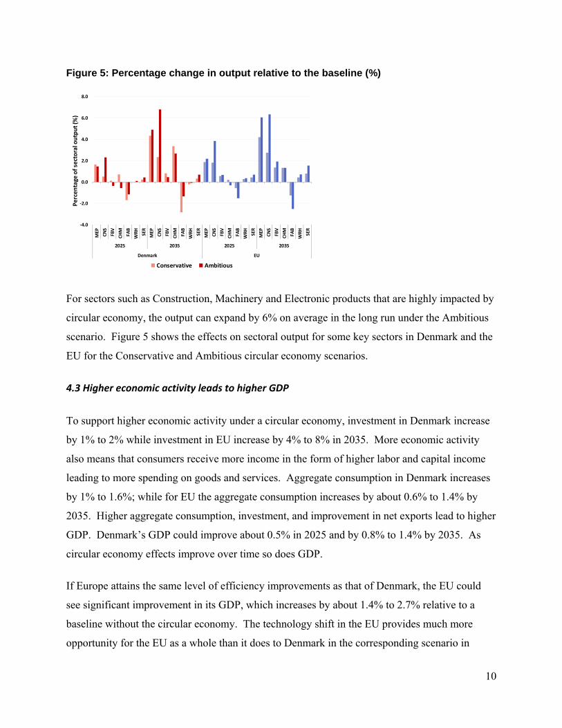
Figure 5: Percentage change in output relative to the baseline (%)
For sectors such as Construction, Machinery and Electronic products that are highly impacted by
circular economy, the output can expand by 6% on average in the long run under the Ambitious
scenario. Figure 5 shows the effects on sectoral output for some key sectors in Denmark and the
EU for the Conservative and Ambitious circular economy scenarios.
4.3 Higher economic activity leads to higher GDP
To support higher economic activity under a circular economy, investment in Denmark increase
by 1% to 2% while investment in EU increase by 4% to 8% in 2035. More economic activity
also means that consumers receive more income in the form of higher labor and capital income
leading to more spending on goods and services. Aggregate consumption in Denmark increases
by 1% to 1.6%; while for EU the aggregate consumption increases by about 0.6% to 1.4% by
2035. Higher aggregate consumption, investment, and improvement in net exports lead to higher
GDP. Denmark’s GDP could improve about 0.5% in 2025 and by 0.8% to 1.4% by 2035. As
circular economy effects improve over time so does GDP.
If Europe attains the same level of efficiency improvements as that of Denmark, the EU could
see significant improvement in its GDP, which increases by about 1.4% to 2.7% relative to a
baseline without the circular economy. The technology shift in the EU provides much more
opportunity for the EU as a whole than it does to Denmark in the corresponding scenario in
‐4.0
‐2.0
0.0
2.0
4.0
6.0
8.0MEP
CNS
FBV
CHM
FAB
WRH
SER
MEP
CNS
FBV
CHM
FAB
WRH
SER
MEP
CNS
FBV
CHM
FAB
WRH
SER
MEP
CNS
FBV
CHM
FAB
WRH
SER
2025 2035 2025 2035
Denmark EU
Percentage of sectoral output (%
)
Conservative Ambitious
11
which the circular economy was created within Denmark only. The EU’s economy is in general
less efficient than Denmark’s and hence we see that the same efficiency improvement in the EU
as a whole provides more benefit to the EU economy as a whole. Figure 6 below shows the GDP
effects for Denmark and the EU in the Conservative and Ambitious scenario over time.
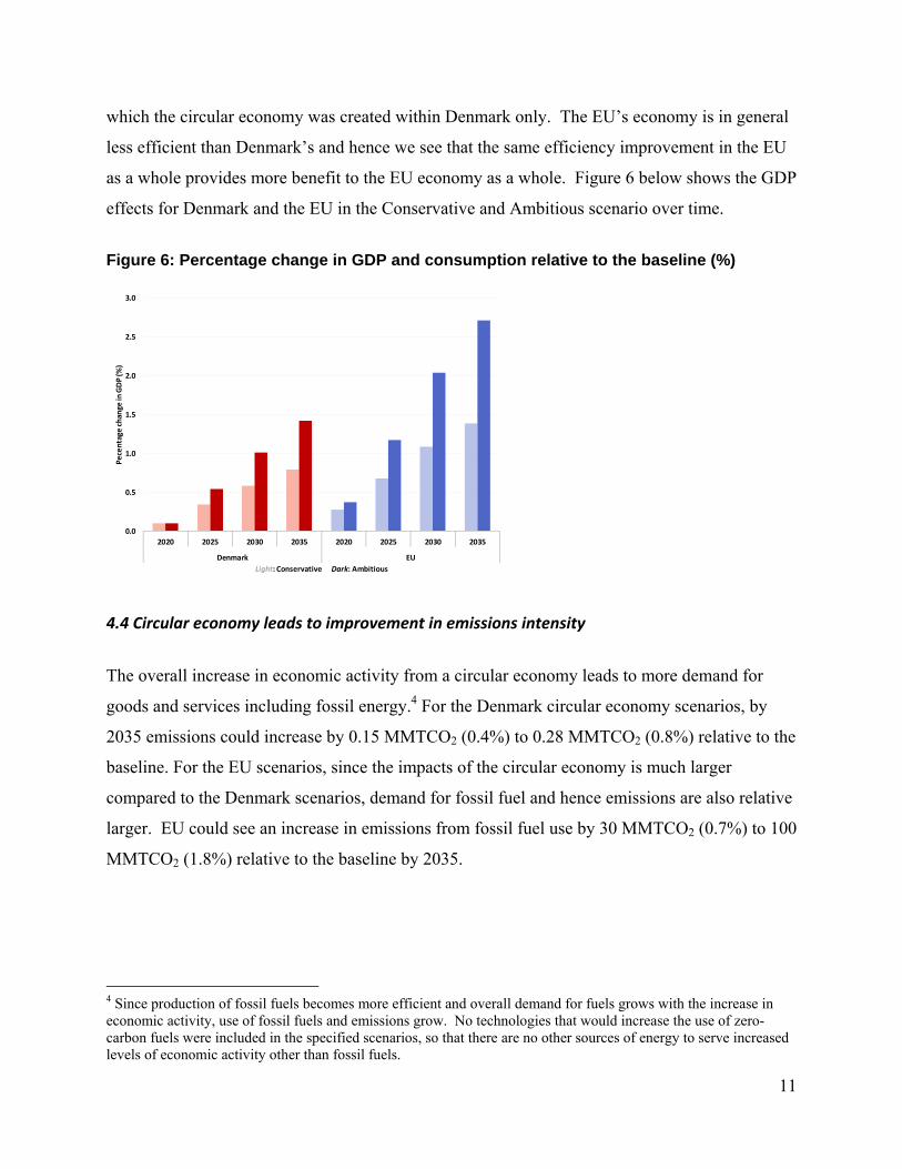
Figure 6: Percentage change in GDP and consumption relative to the baseline (%)
4.4 Circular economy leads to improvement in emissions intensity
The overall increase in economic activity from a circular economy leads to more demand for
goods and services including fossil energy.4 For the Denmark circular economy scenarios, by
2035 emissions could increase by 0.15 MMTCO2 (0.4%) to 0.28 MMTCO2 (0.8%) relative to the
baseline. For the EU scenarios, since the impacts of the circular economy is much larger
compared to the Denmark scenarios, demand for fossil fuel and hence emissions are also relative
larger. EU could see an increase in emissions from fossil fuel use by 30 MMTCO2 (0.7%) to 100
MMTCO2 (1.8%) relative to the baseline by 2035.
4 Since production of fossil fuels becomes more efficient and overall demand for fuels grows with the increase in economic activity, use of fossil fuels and emissions grow. No technologies that would increase the use of zero-carbon fuels were included in the specified scenarios, so that there are no other sources of energy to serve increased levels of economic activity other than fossil fuels.
0.0
0.5
1.0
1.5
2.0
2.5
3.0
2020 2025 2030 2035 2020 2025 2030 2035
Denmark EU
Pecentage
change
in GDP (%
)
Light: Conservative Dark: Ambitious
12
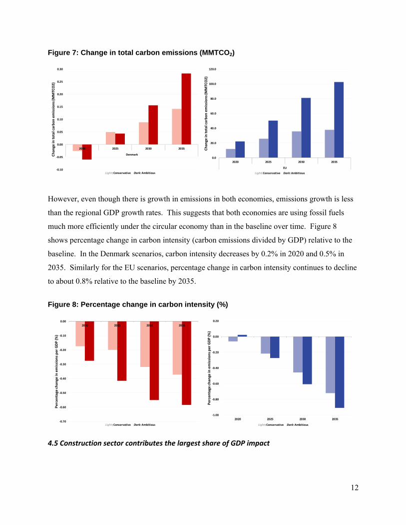
Figure 7: Change in total carbon emissions (MMTCO2)
However, even though there is growth in emissions in both economies, emissions growth is less
than the regional GDP growth rates. This suggests that both economies are using fossil fuels
much more efficiently under the circular economy than in the baseline over time. Figure 8
shows percentage change in carbon intensity (carbon emissions divided by GDP) relative to the
baseline. In the Denmark scenarios, carbon intensity decreases by 0.2% in 2020 and 0.5% in
2035. Similarly for the EU scenarios, percentage change in carbon intensity continues to decline
to about 0.8% relative to the baseline by 2035.
Figure 8: Percentage change in carbon intensity (%)
4.5 Construction sector contributes the largest share of GDP impact
‐0.10
‐0.05
0.00
0.05
0.10
0.15
0.20
0.25
0.30
2020 2025 2030 2035
DenmarkChange in
total carbon emissions (M
MTCO2)
Light: Conservative Dark: Ambitious
0.0
20.0
40.0
60.0
80.0
100.0
120.0
2020 2025 2030 2035
EU
Chan
ge in
total carbon emissions (M
MTCO2)
Light: Conservative Dark: Ambitious
‐0.70
‐0.60
‐0.50
‐0.40
‐0.30
‐0.20
‐0.10
0.00
2020 2025 2030 2035
Percentage change in
emissions per GDP (%)
Light: Conservative Dark: Ambitious
‐1.00
‐0.80
‐0.60
‐0.40
‐0.20
0.00
0.20
2020 2025 2030 2035
Percentage change in
emissions per GDP (%
)
Light: Conservative Dark: Ambitious
13
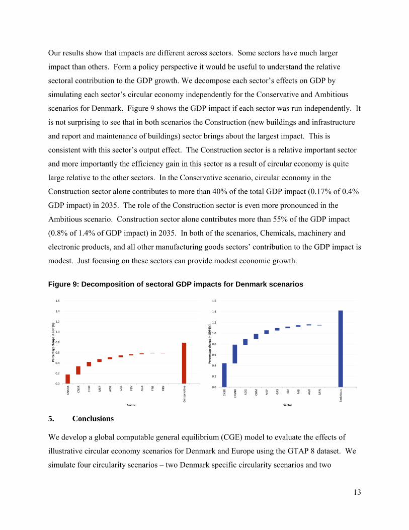
Our results show that impacts are different across sectors. Some sectors have much larger
impact than others. Form a policy perspective it would be useful to understand the relative
sectoral contribution to the GDP growth. We decompose each sector’s effects on GDP by
simulating each sector’s circular economy independently for the Conservative and Ambitious
scenarios for Denmark. Figure 9 shows the GDP impact if each sector was run independently. It
is not surprising to see that in both scenarios the Construction (new buildings and infrastructure
and report and maintenance of buildings) sector brings about the largest impact. This is
consistent with this sector’s output effect. The Construction sector is a relative important sector
and more importantly the efficiency gain in this sector as a result of circular economy is quite
large relative to the other sectors. In the Conservative scenario, circular economy in the
Construction sector alone contributes to more than 40% of the total GDP impact (0.17% of 0.4%
GDP impact) in 2035. The role of the Construction sector is even more pronounced in the
Ambitious scenario. Construction sector alone contributes more than 55% of the GDP impact
(0.8% of 1.4% of GDP impact) in 2035. In both of the scenarios, Chemicals, machinery and
electronic products, and all other manufacturing goods sectors’ contribution to the GDP impact is
modest. Just focusing on these sectors can provide modest economic growth.
Figure 9: Decomposition of sectoral GDP impacts for Denmark scenarios
5. Conclusions
We develop a global computable general equilibrium (CGE) model to evaluate the effects of
illustrative circular economy scenarios for Denmark and Europe using the GTAP 8 dataset. We
simulate four circularity scenarios – two Denmark specific circularity scenarios and two
0.0
0.2
0.4
0.6
0.8
1.0
1.2
1.4
1.6
CNSN
R
CNSR
CHM
MEP
AOG
GAS
FBV
AGR
FAB
MIN
Conservative
Percentage change
in GDP (%
)
Sector
0.0
0.2
0.4
0.6
0.8
1.0
1.2
1.4
1.6
CNSR
CNSN
R
AOG
CHM
MEP
GAS
FBV
FAB
AGR
MIN
Ambitious
Percentage change
in GDP (%
)
Sector
14
scenarios that affect the European Union. The scenarios assume that there are no upfront
economic costs and no opportunity costs of achieving efficiency improvement that defines the
circular economy. The modeling results show that relative to the baseline levels Danish GDP
could increase by 0.8% to 1.4% by 2035. Under similar circular economy assumptions,
European Union’s GDP could rise by 1.4% to 2.7% by 2035. Our sectoral modeling results
show that the construction sector contributes more than half of the GDP growth and the rest of
the GDP growth comes from other sectors that also play an important role in placing the
economy on a sustainable growth path.
15
References
Ayres, R.U., and Kneese, A.V., 1969. “Production, Consumption and Externalities”, American Economic Review 59: 282-297. Bohringer, C. and Rutherford, T.F. 2015. “The Circular Economy – An Economic Impact Assessment,” Report to SUN-IZA Bohringer, C., Rutherford, T.F. and Wiegard, W. 2015. “Computable General Equilibrium Analysis: Opening a Black Box”, ZEW Discussion Paper No. 03-56. http://ftp.zew.de/pub/zew-docs/dp/dp0356.pdf The Ellen MacArthur Foundation. 2015. “Delivering The Circular Economy: A Toolkit for Policymakers.” European Commission. 2015. “Closing the loop – An EU action plan for the Circular Economy,” Communication from the commission to the European parliament, the council, the European economic and social committee and the committee of the regions. Hoornweg, D., and Freire, M., 2013. “ Building Sustainability in An Urbanizing World – A Partnership Report”. Urban Development Series Knowledge Papers. The World Bank. Kang, S. I., Kim, J. J., and Masui, T., 2006. “A National CGE Modeling for Resource Circular Economy”. Korea Environment Institute, WO-02. NewERA Modeling Framework. NERA Economic Consulting. Noll, Roger G., and Trijonis, J., 1971. “Mass Balance, General Equilibrium, and Environmental Externalities”, American Economic Review 61:730-735. Rutherford, T.F. 2005. “GTAP6inGAMS: The Dataset and Static Model”, Ann Arbor, MI. Available at URL: http://www.mpsge.org/gtap6/gtap6gams.pdf Rutherford, T.F. 2002. “Lecture Notes on Constant Elasticity Functions”, http://www.gamsworld.org/mpsge/debreu/ces.pdf Rutherford, T.F. 1995. “Extension of GAMS for complementarity problems arising in applied economic analysis,” Journal of Economic Dynamics and control 19 (8), 1299-1324
16
Appendix A: Description of the Global NewERA Model
The model is written in GAMS/MPSGE. The MPSGE syntax adopts a calibrated share form that
compared to a conventional coefficient form substitutes a set of parameters calculation with the
readily available benchmark values.
A. Production and Trade Structure of Macro Model
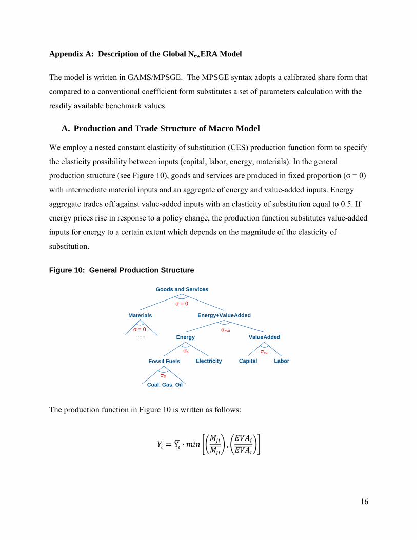
We employ a nested constant elasticity of substitution (CES) production function form to specify
the elasticity possibility between inputs (capital, labor, energy, materials). In the general
production structure (see Figure 10), goods and services are produced in fixed proportion (σ = 0)
with intermediate material inputs and an aggregate of energy and value-added inputs. Energy
aggregate trades off against value-added inputs with an elasticity of substitution equal to 0.5. If
energy prices rise in response to a policy change, the production function substitutes value-added
inputs for energy to a certain extent which depends on the magnitude of the elasticity of
substitution.
Figure 10: General Production Structure
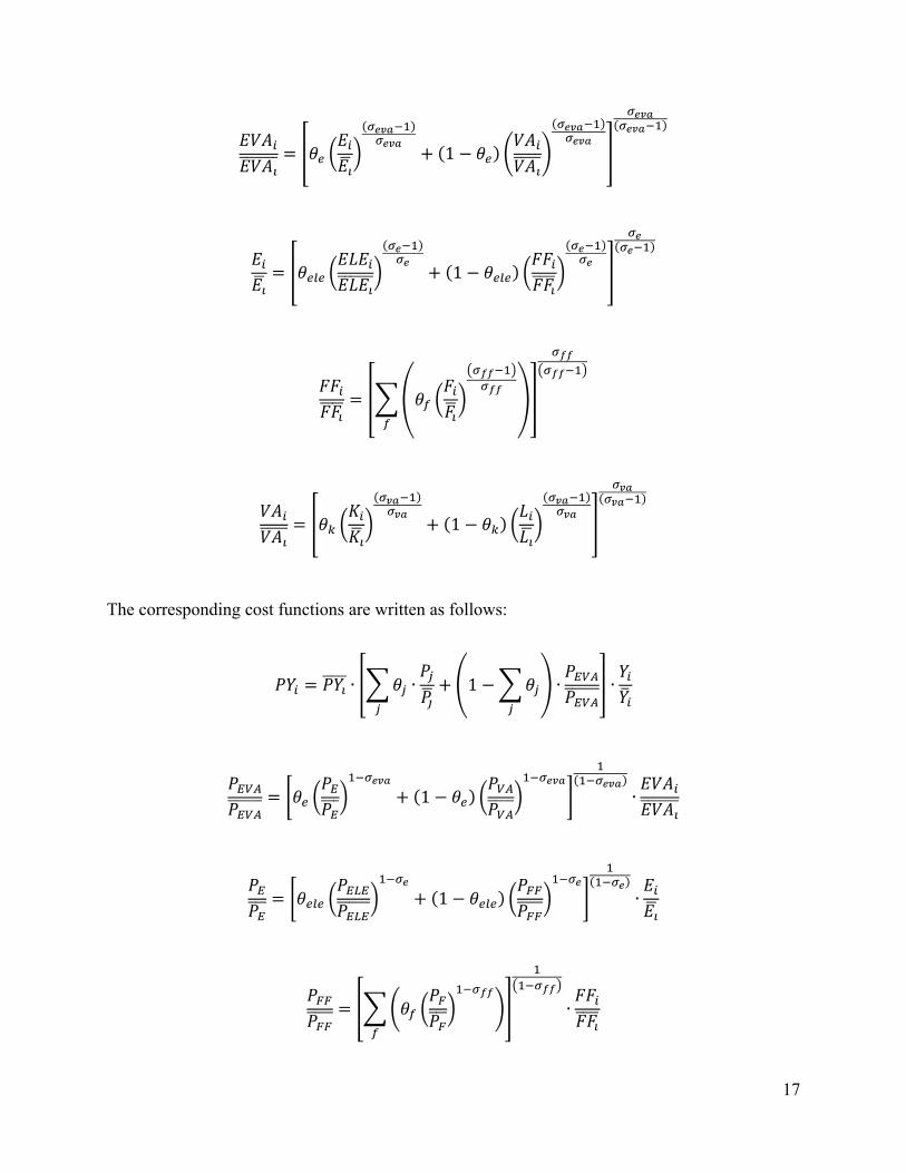
The production function in Figure 10 is written as follows:
Y ∙ ,
Materials
Goods and Services
Energy ValueAdded
Capital LaborFossil Fuels Electricity
Coal, Gas, Oil
σ = 0
σeva
...... σ = 0
σvaσe
σff
Energy+ValueAdded
17
1
1
1
The corresponding cost functions are written as follows:
∙ ∙ 1 ∙ ∙
1 ∙
1 ∙
∙
18
1 ∙
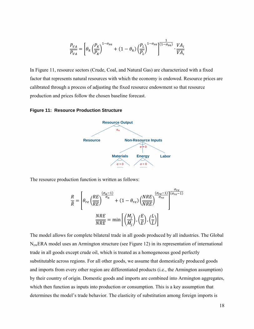
In Figure 11, resource sectors (Crude, Coal, and Natural Gas) are characterized with a fixed
factor that represents natural resources with which the economy is endowed. Resource prices are
calibrated through a process of adjusting the fixed resource endowment so that resource
production and prices follow the chosen baseline forecast.
Figure 11: Resource Production Structure
The resource production function is written as follows:
1
min , ,
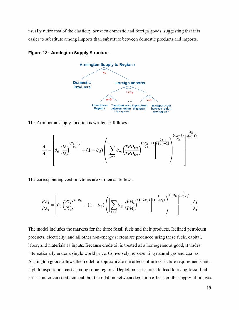
The model allows for complete bilateral trade in all goods produced by all industries. The Global
NewERA model uses an Armington structure (see Figure 12) in its representation of international
trade in all goods except crude oil, which is treated as a homogeneous good perfectly
substitutable across regions. For all other goods, we assume that domestically produced goods
and imports from every other region are differentiated products (i.e., the Armington assumption)
by their country of origin. Domestic goods and imports are combined into Armington aggregates,
which then function as inputs into production or consumption. This is a key assumption that
determines the model’s trade behavior. The elasticity of substitution among foreign imports is
Resource Output
Labor
σrs
......
Materials
σ = 0
Resource Non-Resource Inputs
σ = 0
Energy
……σ = 0
19
usually twice that of the elasticity between domestic and foreign goods, suggesting that it is
easier to substitute among imports than substitute between domestic products and imports.
Figure 12: Armington Supply Structure
The Armington supply function is written as follows:
1
The corresponding cost functions are written as follows:
1 ∙
The model includes the markets for the three fossil fuels and their products. Refined petroleum
products, electricity, and all other non-energy sectors are produced using these fuels, capital,
labor, and materials as inputs. Because crude oil is treated as a homogeneous good, it trades
internationally under a single world price. Conversely, representing natural gas and coal as
Armington goods allows the model to approximate the effects of infrastructure requirements and
high transportation costs among some regions. Depletion is assumed to lead to rising fossil fuel
prices under constant demand, but the relation between depletion effects on the supply of oil, gas,
Armington Supply to Region r
σa
Domestic Products
Foreign Imports
…
2xσa
Import fromRegion i
σ=0
Transport cost between region
i to region r
Import from Region n
σ=0
Transport cost between region
n to region r
20
and coal and the actual supply of these fuels is ignored. That is, the model does not keep a record
of the current stock of each fuel in each time period. World supply and demand determine the
world price of fossil fuels. Current taxes and subsidies are included in each country’s prices.
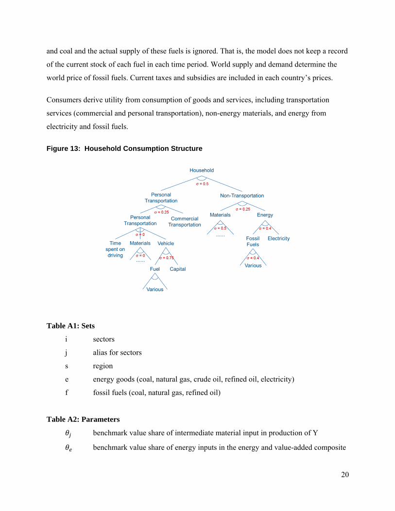
Consumers derive utility from consumption of goods and services, including transportation
services (commercial and personal transportation), non-energy materials, and energy from
electricity and fossil fuels.
Figure 13: Household Consumption Structure
Table A1: Sets
i sectors
j alias for sectors
s region
e energy goods (coal, natural gas, crude oil, refined oil, electricity)
f fossil fuels (coal, natural gas, refined oil)
Table A2: Parameters
benchmark value share of intermediate material input in production of Y
benchmark value share of energy inputs in the energy and value-added composite

21
benchmark value share of electricity in the energy composite
benchmark value share of fossil input in the fossil-fuel composite
benchmark value share of capital in the value-added composite
benchmark value share of resource in the resource production
benchmark value share of imported goods and services from region s to region r
out of all imports
compensated elasticity of substitution between the energy and value-added
composites
compensated elasticity of substitution between electricity and the fossil-fuel
composite
compensated elasticity of substitution between the fossil fuel inputs in the fossil-
fuel composite
compensated elasticity of substitution between capital and labor in the value-
added composite
compensated elasticity of substitution between resource and non-resource input in
the resource production
Table A3: Variables
Market activity
Y productionofnon‐resourcegoodsandservices
R productionofexhaustibleresources coal,gas,crudeoil
M intermediatematerialdemand
A Armingtongoods
D domesticproducedgoodsandservicessuppliedtothedomesticmarket
TRD tradeofgoodsandservices
EVA energyandvalue‐addeddemand
E energydemand
VA value‐addeddemand
ELE electricitydemand
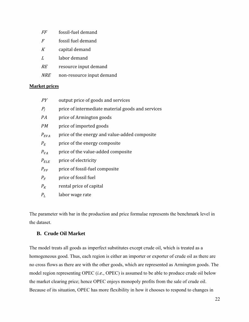
22
FF fossil‐fueldemand
F fossilfueldemand
K capitaldemand
L labordemand
RE resourceinputdemand
NRE non‐resourceinputdemand
Market prices
PY outputpriceofgoodsandservices
Pj priceofintermediatematerialgoodsandservices
priceofArmingtongoods
priceofimportedgoods
priceoftheenergyandvalue‐addedcomposite
priceoftheenergycomposite
priceofthevalue‐addedcomposite
priceofelectricity
priceoffossil‐fuelcomposite
priceoffossilfuel
rentalpriceofcapital
laborwagerate
The parameter with bar in the production and price formulae represents the benchmark level in
the dataset.
B. Crude Oil Market
The model treats all goods as imperfect substitutes except crude oil, which is treated as a
homogeneous good. Thus, each region is either an importer or exporter of crude oil as there are
no cross flows as there are with the other goods, which are represented as Armington goods. The
model region representing OPEC (i.e., OPEC) is assumed to be able to produce crude oil below
the market clearing price; hence OPEC enjoys monopoly profits from the sale of crude oil.
Because of its situation, OPEC has more flexibility in how it chooses to respond to changes in

23
market conditions that result in less demand for crude oil. The approach we take to modeling
OPEC’s response to reduced demand for oil is to construct polar cases. In one case, we maintain
the baseline price by cutting OPEC’s output. In the other case, we keep output at the baseline
level and let the price fall. In the policy scenarios, we assume that the OPEC chooses a middle
ground in which it cuts its output by half of the amount required to maintain price at the baseline
level.