an economic analysis of pre-harvesting marketing
TRANSCRIPT

Louisiana State UniversityLSU Digital Commons
LSU Master's Theses Graduate School
2002
An economic analysis of pre-harvesting marketingstrategies and financial performanceManuel Duarte FilipeLouisiana State University and Agricultural and Mechanical College, [email protected]
Follow this and additional works at: https://digitalcommons.lsu.edu/gradschool_theses
Part of the Agricultural Economics Commons
This Thesis is brought to you for free and open access by the Graduate School at LSU Digital Commons. It has been accepted for inclusion in LSUMaster's Theses by an authorized graduate school editor of LSU Digital Commons. For more information, please contact [email protected].
Recommended CitationFilipe, Manuel Duarte, "An economic analysis of pre-harvesting marketing strategies and financial performance" (2002). LSU Master'sTheses. 743.https://digitalcommons.lsu.edu/gradschool_theses/743

AN ECONOMIC ANALYSIS OF PRE-HARVESTING MARKETING STRATEGIES AND FINANCIAL PERFORMANCE
A Thesis
Submitted to the Graduate Faculty of the Louisiana State University and
Agricultural and Mechanical College in partial fulfillment of the
requirements for the degree of Master of Science
In
The Department of Agricultural Economics and Agribusiness
by Manuel Duarte Filipe
B.S., Universidade Eduardo Mondlane, 1996 December 2002

ii
ACKNOWLEDGEMENTS
I need to thank many people for helping me complete the present work, but the
space allowed for acknowledgements is too limited for mentioning all the people that
need to be thanked. So I would mention the ones that I can, and hope that the ones not
mentioned here also feel thanked for all the support they have given to me.
First of all I would like to express my appreciation to my major professor Dr.
Lonnie Vandeveer for the guidance, patience, understanding, and most of all for making
it possible for me to have a presentable thesis project. Without him this project would not
be what it is.
Second my thanks go to the committee members Dr. Kenneth W. Paxton, Dr.
Michael Salassi, and Dr. Sudipta Sarangi for accepting to serve for this capacity, for
being my source of inspiration, and for being the standard guideline that made me work
to the best of my capabilities. It was thinking in my committee members that I was
pushing my self to the limit. They really inspired me to work for my best. My thanks are
also extended to Dr. Kurt Guidry for the help and support that really made a major
difference for the success of the present study.
To my mother, Julia Duarte Filipe, for the love, support, understanding showed
throughout all these years. I also thank you mum for believing in me, and for giving me
faith to fight through struggles, which was what gave me strengths to be here today
fighting. Rest in peace mum, I will always have you in my heart.
To my brothers Fernando Duarte Filipe and Amandio Albano Manuel that gave
me inspiration and a reason not to fail. I thank you guys.

iii
To my friends: Amade Sene, Anabela Mabota, Farida Saifodine, Elsa Mapilele, Pedro
Sebastiao, Maria Sebastiao, Louana Sebastiao, Bento Quifuma, Irene Graça, Wilker
Vieira, Susana Abreu, Cecilia Abreu, Maristela Abreu, Herberto Lafayete, Paula
Lafayete, Bruno Boamorte, Horacio Comas, and many others close friends that could not
fit in this paper, that were with me on the hours of loneliness and desperation. Friends
that made it possible that I felt home away from home, I extended my deepest
appreciation.

iv
TABLE OF CONTENTS
Acknowledgements…………………………………………………………………….…II
List of Tables………………………………………………………………………….…VI
List of Figures………………..………………………….……………………………….IX
Abstract…………...………………………………………………………………....……X
Chapter I Introduction…………...…………………………………………………………...1
Problem Statement……………………………………………………...…6 Objectives…………………………………………………………………6 Methods and Procedures…………………………………..………………7 Plan of Study…………………………………..…………………………10
II Theory and Literature Review………………………………………………..….11
Production Theory……..……………………………………………...…11 Portfolio Theory……………...……...……………………………...……15 Marketing Theory………………......……………………………………18 Portfolio Selection Criterion Theory…….………………………………21 Literature Review………...…………………………………………...….24 III Procedures and Data…………………………………………..…………………29 Optimal Marketing Portfolio…………………………………………..…29 Optimal Production Portfolio…………………………………….………32 Financial Model...……………………………………………………..…33 Data………………………………………………………………………38 IV Empirical Results………………...……………………………………………....45 Optimal Marketing Strategy………………...…...………………………45 Marketing Strategy Portfolio…………………...………………..………49 Production Portfolio………………………………………………...……54 Sensitivity Analysis…………………………………………….………..58 Financial Implications……………………………………………………64 V Summary and Conclusions………………………………………………………74 General Approach…………...……………………………………...……75 Data and Procedures……………...…………………………...…………76 Results ………………………………………………………..………….78 Limitations of the Study……………………………………………….…80 Conclusions………………………………………………………………82

v
References……………………………………………………………………………..…84 Vita……………………………………………………………………………………….86

vi
LIST OF TABLES Table Page
1. U.S. farm sector cash receipt from sales of agricultural commodities, 1997 -2000 ($Billion)…..……………………………………………….…………..…….4
2. Unadjusted and adjusted prices for corn under different
marketing strategy scenarios, central Louisiana, 1986-1999………..……..…….40 3. Unadjusted and adjusted prices for Soybeans under different marketing strategies,
central Louisiana, 1986-1999…………………….…………………..…………..42 4. Corn yield and estimated gross rate of return on assets,
central Louisiana, 1986 – 1999……..……………………………………………43 5. Soybeans yield and estimated gross rate of returns on assets, central
Louisiana, 1986 – 1999…………………………………………………………..44 6 Estimated corn percentage gross rate of return on assets,
central Louisiana, 1986 –1999….…….…………………………………………46 7 Estimated soybeans percentage gross rate of return on assets
central Louisiana, 1986 – 1999…………....……..…...………………………….47 8 Estimated relevant marketing strategies correlation coefficients for corn,
central Louisiana, 1986 – 1999……………………………………………….…48 9 Estimated relevant marketing strategies correlation coefficients
for soybean, central Louisiana, 1986 – 1999 ……………...…..………...……....48 10 Estimated relevant marketing strategy correlation coefficient
for corn –soybeans cross combinations, central Louisiana, 1986 – 1999…..………………………………….…….……………..49
11 Optimal marketing strategy portfolio, central
Louisiana corn-soybean farm, 1986 – 1999……………...……………………....50 12. Estimated optimal marketing strategy gross return ($/Acre)
percentage return and distribution, central Louisiana corn-soybean farm, 1986 – 1999………………………………..……………………………....52
13. Estimated gross Rate of return to asset for corn and soybean
farm under traditional cash on spot marketing strategy under, optimal marketing strategy scenarios central Louisiana, 1986 – 1999……………………………………………………………………... 53

vii
14 Estimated net rate of return to asset distribution for
cash and optimal marketing portfolio scenario, central Louisiana, corn-soybean farm, 1986 – 1999………………………………………..…….....53
15 Estimated optimal production portfolio, central Louisiana
corn-soybean farm, 1986 – 1999………………………………………………...55 16 Estimated production portfolio statistics, central Louisiana corn-soybean
farm, 1986 -1999…………………………………………………………………58 17 Sensitivity analysis results estimated for optimal marketing
strategy in a scenario of increasing variable costs for corn production, central Louisiana corn-soybean farm, 1986 -1999………….…59
18 Sensitivity analysis results estimated for optimal marketing strategy in a scenario of decreasing variable costs for corn production, central Louisiana corn-soybean farm, 1986 -1999……………………………………………..……….………….60
19 Sensitivity analysis results estimated for optimal marketing
strategy in a scenario of increasing standard deviation for corn production, central Louisiana corn-soybean farm, 1986 -1999………...….61
20 Sensitivity analysis results estimated for optimal
marketing strategy in a scenario of decreasing standard deviation for corn production, central Louisiana corn-soybean farm, 1986 -1999………………………………...…….61
21 Sensitivity analysis results estimated
for optimal marketing strategy in a scenario of increasing variable costs for soybean production, central Louisiana corn-soybean farm, 1986 -1999………..………..62
22 Sensitivity analysis results estimated
for optimal marketing strategy in a scenario of decreasing variable costs for soybean production, central Louisiana corn-soybean farm, 1986 -1999…..……………………………………………...63
23 Sensitivity analysis results estimated for
optimal marketing strategy in a scenario of increasing standard deviation for soybean production, central Louisiana corn-soybean farm, 1986 -1999………………………………………...………..63
24 Sensitivity analysis results estimated for optimal
marketing strategy in a scenario of decreasing

viii
standard deviation for soybean production, central Louisiana corn-soybean farm, 1986 -1999………………………………64
25 Capital structure, financial parameters, and financial performance estimates, central Louisiana corn-soybean farm, 1999……………………….….66 26 Financial parameters, and financial
performance estimates for cash on
spot marketing strategy, central Louisiana corn-soybean farm, 1986-1999………………………………….……67
27 Financial parameters, and financial performance estimates for optimal marketing strategy, central Louisiana corn-soybean farm, 1986-1999………………..…….69
28 Comparison of financial performances between cash on spot marketing strategy and optimal marketing strategy, central Louisiana 1986 – 1999……………………………...70

ix
LIST OF FIGURES
Figure Page
1 US farm cash expenses and return to risk and management for corn 1975-2000……………………………………………………….……………………….2
2 US farm cash expenses and returns to risk and management for
soybeans 1975-2000…………...…………………………………………….…….3
3 Net farm income and grain crops gross income Louisiana 1970-2000………...…5
4 Hypothetical efficient production point determination…..……………………....14
5 Portfolio possibility frontier…………………………………………………...…18
6 Optimal production portfolio under cash marketing strategy, central Louisiana corn-soybean farm, 1986-1999………...……………………………..57
7 Optimal production portfolio under optimal marketing strategy, central Louisiana corn-soybean farm, 1986-1999…...…………………..………57
8 Estimated debt repayment capacity under certainty conditions, cash and optimal marketing scenarios, Louisiana corn-soybean farm, 1986 - 1999……..……………………..………...71
9 Estimated debt capacity under risky conditions, cash and optimal marketing scenarios, Louisiana corn-soybean farm, 1986 - 1999…….……………………………..…72
10 Financial performance measures for cash and optimal marketing strategies, representative farm, central Louisiana, 1986-1999………..…………73

x
ABSTRACT
Risk is an important concern in the management of a farm business. The rising
input prices along with the variability in the farm commodity prices may result in a risk
environment. Government programs have generally provided income support to farmers.
However, there has been considerable discussion regarding this support in recent years.
The farm act of 2002 and farm bill of 1999 are good examples of such discussions. These
uncertainties emphasize the need to improve information for farm’s income risk
management, and make some one ask if there is not out there any alternative way of
managing income risk besides government intervention.
The literature shows that marketing strategies may be used to improve income
risk management on farmers. This study is aimed at showing how pre-harvest marketing
strategies may be used to manage income risk, using a portfolio approach in which three
chosen marketing strategies are combined in a portfolio. The optimal marketing strategy
combination is estimated assuming a safety first decision model. The optimal marketing
strategy is then used to estimate optimal production portfolio under the specified
scenarios. Cash marketing and optimal pre-harvest marketing scenarios are then
evaluated in a financial model.
Results generally indicate that opportunity to improve farm profitability, liquidity,
and risk exist for the optimal pre-harvest marketing strategy. Results indicate that the
optimal marketing strategy would include for the corn case 24% cash on spot marketing
strategy, 54% forward contract marketing strategy, and 22% hedge to arrive marketing
strategy. For the case of Soybean, the optimal marketing strategy would include 37%

xi
cash on spot marketing strategy, 30% forward contract marketing strategy, and 33%
hedge to arrive marketing strategy.
Comparison between optimal pre-harvest marketing strategy and cash on spot
marketing strategy shows that the optimal pre-harvest marketing strategy has higher rate
of returns to assets and equity, high debt repayment capacity, lower level of risk, higher
level of liquidity, and represents a situation in which farmers has higher level of
probability of repaying debt in nine out of 10 years.

CHAPTER I
INTRODUCTION
The problem of price and income instability in agriculture dates back to the
advent of commercial agriculture in the U.S. In fact agriculture is inherently risky. Output
from the farm in most cases depends on weather and biological processes over which
producers have little control (Fleisher, 1990).
Besides the environmental issues surrounding the agriculture production sector,
its structural characteristics are capital intensive where both leasing and credit are
extensively used to acquire resources for production. The agricultural production sector
also operates in an environment of volatile input and output markets, risky production
environment, and policy uncertainties. These factors create a complex risky climate
(Barry et al., 1995). The producer is faced with the challenge of acquiring and combining
resources within the firm to increase the welfare of the business and at the same time
protect the farmer’s equity within the business.
After reviewing the financial experience of the agricultural sector over several
decades, Melichar 1984, found that farm financial problems began in 1980’s when farm
commodity prices failed to advance while prices in general continued to increase at a
rapid rate. Since then, much attention was devoted to farm financial distress. The 1985
financial survey of farmers in Maine revealed that over one half of the respondents were
planning to leave farming within the next five years. Among these quitting farmers, only
16.7% where leaving for retirement reasons, the rest where leaving because of financial
problems and low profitability in agriculture (Swanberg and Marra, 1987). Although
farm conditions tended to improve in the 1990’s, they continued to be characterized by

2
high input costs, low commodity prices, low price supports, which resulted in tight cash
flow conditions, (Ahrerendsen, 1995).
Trends in cash expenses and profitability for U.S. corn and soybeans as presented
by the USDA agricultural statistical data are presented in Figures 1, 2 and 3. Figure 1
shows the general upward movement in total nominal cash expenses between 1975 and
2000, while per acre profit levels (residual nominal returns to risk and management)
declined for the same period.
-200-100
0100200300400500
1975
1980
1985
1990
1995
2000
Years
$/Pl
ante
d ac
re
Total cash expenses Residual returns to risk and management
Figure 1. US Farm cash expenses and return to risk and management for corn, 1975-2000
Source: Agricultural Income &Finance outlook/AIS-77-Sepember 2001

3
Farm nominal cash expenses and nominal profitability estimates for soybeans in
the U.S. are shown in Figure 2. Estimates presented in Figure 2 generally show a slight
decline in residual (profits) on farmers from 1975 to 2000 with a sharp decline after 1997.
-100
0
100
200
1975 1980 1985 1990 1995 2000Years
$/pl
ante
d ac
re
Total cash expenses Residual returns to management and risk
Figure 2 .US farm expenses and return to risk and management for soybeans, 1975-2000
Source: Agricultural Income &Finance outlook/AIS-77-Sepember 2001.
Nominal cash receipts for corn and soybeans are presented in Table 1. Estimates
in Table 1 indicate both variability and downward trends in cash receipts for both corn
and soybean enterprises. USDA estimates of gross receipts (Table 1) for commodities
also show similar downward trend. Data presented in Table 1 show that the nominal cash
receipts from sales of farm crops continued trending downward in the last five years.

4
Table 1: U.S. farm sector cash receipt from sales of agricultural commodities, 1997 -2000 ($Billion)
Item/Years 1997 1998 1999 2000
Corn 20.0 17.2 14.8 15.5
Soybean 18.1 15.6 12.0 12.5
Total Crops 111.2 101.7 92.6 94.1
Source: Economic Research Service, USDA - Agriculture Income and Finance Outlook, September 2001.
The agriculture income situation in Louisiana has been characterized by having a
great deal of variability through out the years. Income estimates presented in Figure 3
show that the Louisiana’s production sector has been characterized by income variability,
(1970-2000). Net farm income and grain crop gross income for the farm production
sector are shown in Figure 3. Trends presented in Figure 3 indicate substantial variability
in farm income over the period 1970 – 2000.
Throughout the years, farm income risk has been a problem that farmers,
researchers, and policy makers cannot easily dismiss. In fact through out the years, the
government has supported farmers in dealing with income risk by using different policy
tools such as direct payment, and price support programs.
In a Nebraska farmer’s survey, Johnson 1996 found that the most common risk
management strategy among farmers was government program participation. However,
policy swings from time to time poses concerns regarding a need for an alternative risk
absorbing mechanism in agriculture. According to the ERS farm bill publication
summary, the 1996 farm act and the 2002 farm bill show two different scenarios of

5
0200,000400,000600,000800,000
1,000,00019
7019
7419
7819
8219
8619
9019
9419
98
Years
$100
0
net farm income
grain crop grossincome
Figure 3 Net farm income and grain crops gross income, Louisiana, 1970-2000
Source: Agricultural Income &Finance outlook/AIS-77-Sepember 2001
government support programs in agriculture. The first act attempted to support the
phasing out of the government intervention, and the other attempts to support the
“phasing in” of the government intervention in Agriculture. Situations like this leads one
to question if there are alternative ways of managing income risk beside government
programs. In fact, the back and forth swing in policy suggests a need for farmers, as well
as politicians, and decisions makers, to have a wider range of income risk management
tools.
A nationwide survey by Koo, et al., (1998) indicates that in the absence of
government programs, 40% of farmers suggested they would increase the use of

6
marketing tools to increase their returns, 28% would use production contracts, which also
is a marketing strategy. Barry, et al., 2000 argues that marketing alternatives provide
farmers with methods for risk management. Marketing alternatives that have been
mentioned are cash on spot selling strategy, forward contracting strategy and hedge to
arrive contracting strategy. While it is generally recognized that farmers can use
marketing strategies to manage risk, there are few studies that show how improved
marketing strategies can improve farm financial performance.
Problem Statement
It is frequently stated that marketing strategies can provide a way of managing
income risk in the farm business; however, there are few studies in the literature about
how these marketing strategies can be effectively combined in one useful “package” so
that farmers can easily use them to improve their financial conditions and manage risk.
Howard et al. note that forward contracting not only can have favorable diversification
benefits in the current year, but can reduce price uncertainty in future years. An important
question concerns the relationship of pre-harvest marketing strategies and farmers
financial performance. More specifically, what is the relationship between pre-harvest
marketing strategies and financial performance measures such as farm profits, risk and
liquidity? A study aimed at estimating the effect of alternative marketing strategies on
farm financial performance is expected to provide important information to those
interested in the financial performance of the farm firm.
Objectives
The general objective of this study is to examine the relationship between pre-
harvest marketing strategies and financial performance measures (profit, liquidity, and

7
risk) of a representative soybean-corn farm in central Louisiana. The specific objectives
are: 1. To identify a representative grain crop farm in central Louisiana ; 2. To identify
pre-harvest marketing strategies for selected grain crops in central Louisiana; 3. To
estimate the rate of return to asset distributions for selected pre-harvest marketing
strategies for the selected grain crops in the study area; 4. To develop a modeling
procedure for estimating the relationship between marketing decisions and production
decisions; 5. To estimate the effect of pre-harvest marketing decisions, on the financial
performance of a representative farm in the targeted area.
Methods and Procedures
Specific Objective Number One :
To identify a representative grain crop farm in Louisiana, the study reviewed farm
budgets, rural land and survey data, along with data from Louisiana’s Farm Bureau
statistics. It was aimed at finding the most common type of farm in terms of acreage and
assets, and the most common crops.
Specific Objective Number Two:
The identification of the pre-harvest marketing strategies for selected grain crops
in the study area, involved interviews with marketing extension specialists. Also a
collection of information from local elevators about the more predominant marketing
strategies in use for the relevant grain crops in Louisiana was done.
Specific Objective Number Three:
The objective three requires that rate of return distribution be estimated for the
representative grain crops identified in objective one and for selected pre-harvesting
marketing strategies identified in objective two. The estimation of the rate of return to

8
asset distributions for the selected pre-harvest marketing strategies and for the selected
grain crops involved getting yield data from the National Agricultural Statistics Service
reports and prices from Louisiana Farm Bureau Marketing Service. These data sets were
used to calculate gross returns on the selected grain commodities on each marketing
strategy and their respective distributions (mean and standard deviation). The data was
tested for trend and for normality.
Specific Objective Number Four:
Objective four requires a model that links the relationship between marketing
decision and production decisions. At the heart of the analysis is the estimation of
optimal pre-harvest marketing scenarios. Roy’s safety-first decision criterion is assumed
in the analysis. According to Elton, and Gruber, Roy’s safety first decision criterion states
that the optimal portfolio is the one that presents the smallest probability of producing a
return below some specific critical level. If RP is the return on the portfolio and RL is the
critical level below which the investor does not wish returns to fall. The Roy’s criterion is
represented as:
Minimize Prob (RP, RL) (1)
The Roy’s safety first model is used to build an objective function used in a
nonlinear programming procedure to estimate the optimal marketing strategies. Once an
optimal pre-harvest marketing strategy is estimated, the rates of return distributions are
estimated for farm enterprises. This information is then used to estimate the optimal farm
enterprise production portfolio. Non linear optimization procedure is used to estimate
optimal production portfolio

9
In general, the results of the study are estimated in two steps. The first step is to use
the Roy’s safety first model to estimate the optimal marketing portfolio. The second step
is to apply the results from steps one and use the Roy’s safety first model to estimate the
optimal production portfolio.
Specific Objective Number Five :
Optimal marketing and production portfolio estimates are used in a financial
model to develop financial performance estimates. More specifically, profitability,
liquidity, and risk estimates are developed for a 1,000 acre corn soybean representative
farm. Financial estimates from a traditional marketing scenario are compared to such
estimates developed under the optimal marketing scenario.
The level of profitability associated with each marketing strategy scenario is
estimated by the mean rate of return to equity capital, which is estimated from the
financial model. The level of liquidity is estimated by summing the rate of return to
equity generated by the marketing strategies (profitability) and the credit reserve. The
level of credit reserve is estimated by subtracting the level of maximum debt allowed for
each marketing strategy scenario and the assumed actual level of debt for the same
marketing strategy scenario.
Within the safety first framework, it is assumed that the decision maker wishes to
meet all financial commitments for a given probability level. This requirement is met by
using a three equation model that estimates maximum debt repayment capacity.
Maximum debt repayment capacity is estimated as a leverage level where the required
rate of return to equity under risky condition is equal to the rate of return to the equity
capital. The actual level of debt is externally given at a certain assumed level.

10
This study is expected to provide the basis for explaining the relationship between
farm marketing, production, and financial decisions. The specific steps to achieve that are
outlined in the coming chapters.
Plan of Study
The discussion included in the next chapter (chapter two) presents the theoretical
considerations and framework regarding the issues being analyzed in the present study.
A review of previous research is also presented in this chapter. The review of previous
research summarizes basic findings and provides a basis for this research. Studies done
by other authors are presented in the mentioned chapter. The focus on the mentioned
literature review is on the approach, and methodology used by other authors as well as
the results they found in their research work.
The modeling procedures are presented in chapter three. In this chapter, the
concepts, methodology, and procedures used in the study are outlined. Concepts,
formulas, and explanations of the meaning of the technical vocabulary are also presented.
The results of the analyses are presented in chapter four. Here the discussion
includes graphics, Tables and interpretations of the results found by the study.
The summary and conclusions are presented in chapter five. Major findings of the
study as well as suggestion for future research are presented and discussed in this chapter.
11
CHAPTER II
THEORY AND LITERATURE REVIEW
The discussion in this chapter presents the theoretical framework of the subjects
covered in this study. This chapter also presents the work completed by other authors
regarding the subject matter of the present study.
Production Theory
The theory of production suggests that in the production process firms transform
inputs into outputs. Inputs include anything that the firm must use as part of the
production process. The relationship between the inputs to the production process and the
resulting output is described by a production function. A production function indicates
the highest amount of output that a firm can produce for every specified combination of
inputs.
In the present study the firm is assumed to have a production function in which
two products are produced, corn and soybeans. The inputs are assumed to be infinitely
available and the input and output market are assumed competitive. The problem to be
analyzed involves finding the optimal production mix for the two product firm.
According to Pindyck and Rubinfeld, in producing two outputs, managers must
decide how much of each product to produce. The curve showing the various
combinations of two different outputs that can be produced with a given set of inputs
holding technology constant is called the production possibility frontier. This is a
negative sloped curve. Its slope increases in magnitude as more of the horizontal axis
good is produced. The production possibility frontier is concave. The concept that defines
how much of one product (the one in the vertical axis) must be given up in order to

12
produce one extra unit of the other product (the one on the horizontal axis) is called
marginal rate of transformation. If for example in the present study case, the amount of
soybean produced is put on the horizontal axis and the amount of corn on the vertical
axis, the marginal rate of transformation of soybean for corn at a given point is the slope
of the production possibility frontier at that specified point.
As the production moves along the production possibility frontier, the marginal
rate of transformation changes. It is because the productivity of producing each one of the
goods changes as the allocation of inputs changes. The marginal rate of transformation
also measures the marginal cost of producing one good relative to the marginal cost of
producing the other good.
The production possibility curve is important for understanding the economics of
determining the efficient output in a production mix. Pindyck and Rubinfeld state that,
for the production of goods to be efficient, goods must not only be produced at minimum
cost, but they must also be produced in combinations that match buyer’s willingness to
pay for them. To understand this it would be important to mention that the marginal rate
of substitution of soybean for corn measures the buyer’s willingness to pay for an
additional unit of soybean by having less corn. Also the marginal rate of transformation
measures the cost of an additional unit of soybean in terms of producing less corn.
When output markets are competitive, all buyers allocate their budgets so their
marginal rates of substitution between two goods equals to the price ratio. The optimal
production level of corn and soybean is then defined by:
MRS = Ps / Pc (2)
Where:

13
MRS = Marginal rate of substitution
Ps = Price of soybean
Pc = Price of corn
At the same time, each profit maximizing firm will produce its output up to the
point at which price is equal to the margina l cost. For the corn-soybean farm, output
levels are defined by:
Ps = MCs and Pc = MCc (3)
Where:
MCs = Marginal cost for soybean
MCc = Marginal cost for corn.
It is known that the marginal rate of transformation is equal to the ratio of the marginal
costs of production, so for the soybean corn case it follows that:
MRT = MCs/MCc = Ps/Pc = MRS (4)
Assuming competitive markets, efficient production occur s where MRT equals MRS.
Production efficiency for the corn-soybean example is illustrated in Figure 4.
Hypothetical production possibility curve, price ratio line, and buyer’s indifference curve
are illustrated in Figure 4. As illustrated in Figure 4, optimal production occurs at point A
where MRT = Ps/Pc. At this level, C1 acres of corn are produced and S1 acres of soybean
are produced.
Economists generally assume that managers organize production to maximize
profits. Firm’s profit is the difference between the firm’s revenue and its cost. Although
firms are always seeking profits, they produce only if revenues are above average
variable costs.

14
0 S1 Soybean (Acres)
Figure 4: Hypothetical efficient production point determination
In economic studies, it is generally assumed that technology of production is
known and it is assumed that the firm’s main goal is to make profits. It is also assumed
that knowledge about economics and production environments are known with certainty.
Technology is assumed to be constant, and that the economic and technologic processes
occur in a timeless fashion.
Corn (Acres)
Price ratio line
Buyers Indifference curve
Production Possibility frontier
Efficient production point
C1 A

15
While profit maximization is important, some question the assumptions of known
prices and production. If these assumptions are released, then decisions are examined in a
risk environment.
Portfolio Theory
Modern portfolio theory recognizes the trade off between profits and risk.
Generally more profitable alternatives are associated with higher levels of risk. For each
investor this trade off varies according to the investors risk preference. There are
investors that are risk lovers, there are investors that are risk averse, and there are
investors that are risk neutral. The assumption that is generally accepted is that most of
investors are risk averse, and that they want to maximize profit at the lowest possible
risk. One way to achieve that is by investing in several different investments. When
investments have returns that are negatively correlated there is a chance to manage risk.
Investors use diversification of investment as a strategy for reducing risk in a
portfolio, holding more than one investment. An interesting question is how do investors
decide about what investments to include in a portfolio? Or what characteristics of a
portfolio are to be considered in a portfolio analysis.
Portfolio analysis requires the estimation of mean return on a portfolio. The mean
return on a portfolio of assets is simply a weighted average of the return on the individual
assets. The weights applied to each return are the fraction of the portfolio invested in that
asset. If RPj is the return on the portfolio and Xi is the fraction of the investor’s funds
invested in the ith asset and Rj the average rate of return from the individual asset, then
RPj = S XiRi (5)

16
The expected return is also a weighted average of the expected value of the
expression just given for the return on the individual assets. The second summary
portfolio characteristic is the variance. The variance of a portfolio designated by s 2P is
simply the expected value of the squared deviation of the returns on portfolio RP from the
mean return on the portfolio, which can be estimated by the following formula:
s 2P =X1
2 s 21 +X2
2 s 22 +2X1X2 s 2
12 (6)
Where:
s 2P = The variance of the portfolio.
s 2i =The variance of the ith investment.
s 2ij = Covariance between investments i and j
Xi = The proportion of investment i in the portfolio.
The standard deviation of the portfolio is given by the square root of the variance
equation.
According to Barry et al. 2000, “A portfolio is a mix or combination of assets,
enterprises, or investments. It is often used to describe holding of financial assets such as
stocks and bonds. However, it also can be applied to holdings of tangible assets such as
grain inventories, growing crops, livestock, machines, lands, and apartment buildings.
The portfolio model indicates how different combinations of investments may reduce an
investor’s risk more than having a single investment”.
Farmers have used various strategies for managing risk. These strategies are
needed for managing farm income variability. In the present study, pre-harvesting
marketing strategies are used to manage income risk. Marketing strategies are used as
risk management strategy because they offer the alternative of lowering income

17
variability by lowering price variability. Thus, this implies that both income and income
variability are important in the analysis. Here, it is assumed that decision makers are
concerned not only with profits but also with risk or income variability. Consistent with
this assumption, a portfolio approach model can be used for evaluating the effect of
marketing strategy on income variability. Portfolio analysis is concerned with finding the
most desirable group of security, investments, or enterprises to hold, given their
properties (Elton and Gruber, 1984). The portfolio model is not only concerned with
measuring the rate of return for various portfolios but with variance of the corresponding
portfolios. From the portfolio analysis, an efficient frontier is developed that plots all
possible points where rational decisions makers can produce. The portfolio possibility
frontier consists of the mean and variance or standard deviations plotted for the efficient
portfolios of securities, investments, or enterprises. The efficient portfolio possibility
frontier is illustrated in the next Figure 5. The risk efficient portfolio set presented in
Figure 5 illustrates the trade off between risk and returns among different investments
and enterprises. The risk efficient portfolio set curve is concave and illustrates the
expected income and standard deviation of income for different portfolio of investments.
As illustrated in the Figure 5, the optimum portfolio is the one that has the highest
return and lowest risk among the securities on the efficient portfolio possibility frontier.
The optimal portfolio coincides with the point in which the line given by standard
deviation equation when it equals zero, touches the portfolio possibility frontier. That is
the point on the line s P = 0 that touches the portfolio efficient frontier (point A in the
graphic). So point A gives the highest return for that level of risk and investment.

18
Returns
Rp
0 σP STDV
Figure 5: Portfolio possibility frontier.
Marketing Theory
An important concern to a producer is the means of marketing production.
Development of optimal marketing strategies is expected to increase returns to the
business, and to increase financial performance.
Marketing is the area of economics that deals with exchange of goods and
services as well as the evaluation of these goods and services. The exchange process is
performed through the physical movements and transformation processes. Through these
The best portfolio
The line of Returns =F(s P)
Risk efficient portfolio set
A

19
processes, areas such as efficiency of transportation and efficiency of production are
often examined. (Guidry, 1993)
For the present study the efficiency of transportation is not to be considered
because the products are assumed not to be transported or to be transported at the highest
efficiency possible. The evaluation of the products and services in question is manifested
in the pricing of them. Here pricing efficiency as a component of marketing is examined
to determine the proper pricing strategy and hence the proper marketing strategy to be
employed.
Marketing can be viewed to be related to production because utility is created
through the physical movement and transformation processes. Another view that can also
be applicable is in a functional approach that includes transportation, storing, processing,
advertising, collecting and disseminating market news, standardizing, grading,
inspecting, financing, and risk bearing. The risk bearing approach of the marketing is of
great interest for the present study.
Guidry states that in the market economy, competitively determined prices are the
guiding force that gives direction to what is produced, what technology is used in
production, where production takes place, when production is carried out, when and
where consumption takes place, and who gets the proceeds from the whole process. If
markets do not operates efficiently, resources used in production may be misallocated,
consumers may not have goods available in the form, quantity, quality, place, and time
desired, and inequalities may occur in the distribution of income among participants in he
marketing process.

20
Marketing as the force that regulates a considerable portion of the economy is to
be explored in this study. The risk bearing ability that marketing can exhibit is of relevant
importance here.
Although there are many different marketing strategies, this study is primarily
concerned with pre-harvest marketing strategies. Pre harvest marketing strategies for this
study are cash on spot strategy, forward contract strategy, and hedge to arrive strategy.
Cash on spot strategy is the traditional selling that the farmers do when the crop is
harvested for direct cash earning.
Forward contract also known as “booking” is by far the most common advanced
pricing strategy used by producers. Cash forward contracts are relatively easy to use and
understand, they eliminate all risks associated with price and basis (difference between
futures and cash prices), and generally offered at all grain elevators. With cash forward
contract, the producer and the elevator agree upon a price that the elevator will pay to the
producer for a given quantity and quality of grain delivered during a specified time. Once
the elevator and producer agree upon the price and enter the contract, the producer has
effectively eliminated all risk (both price and basis risk). Regardless of where prices
move in the future, the producer is guaranteed the price established in the cash forward
contract.
While the producer has eliminated price risk, there is still production risk that
must be faced. Under the agreements of the cash forward contract, the producer is
obligated to deliver a certain quantity of grain on the agreed date. If the producer is
unable to fill the contract, he/she will generally be forced to pay some penalty. The
severity of the penalty and course of the action taken by the elevator will vary by

21
elevator. As a result, when entering the cash forward contract, producers should carefully
read all of the specifications of the contract.
Hedge to arrive contracts allows the producer to eliminate some risk but still
offers the flexibility of establishing the value of the crop at some later date. Hedge to
arrive contracts are linked to a specified futures market contract. The producer and
elevator establish the price of the futures market contract and then the producer has a
specified amount of time to set the basis level. Hedge to arrive contracts generally specify
the quantity and quality of grain to be delivered, a delivery date, and the length of time
the producer has to set the basis level.
Generally, the futures price that is agreed to is the closing price of the futures
market contract linked to the hedge to arrive contract. Once the futures price is agreed to,
the producer then has a specified amount of time to set the basis. Generally, producers set
the basis by simply accepting the closing day basis level. In addition, elevators will often
require that the producers set the basis and make delivery on the same day. As a result,
the producer, must not only watch movements in basis, but also consider when they will
have cash requirements that will require them to make delivery and take payment.
Hedge to arrive contract generally do not take delivery of the grain until the basis
is set and therefore do not offer any type of cash advance. While there may be some
elevators that do allow early delivery, most do not offer a cash advance.
Portfolio Selection Criterion Theory
This study is aimed at identifying optimal marketing portfolios for the business.
Here, different marketing strategies are combined in a portfolio “package”. In analyzing

22
the financial implications of adopting the optimal marketing strategy a safety first
decision criterion is assumed.
There are several different approaches for estimating an optimal portfolio. One
approach is the broadly advocated expected utility approach. In this model, the optimal
portfolio is defined where the investor risk- less investment line is tangent to the risk
efficient frontier. This is the Roy’s safety fist criterion approach.
Roy’s safety first model is appealing for the present study because the concept of
safety first model appears to be consistent with the decision makers concern of meeting
all financial commitments including debt repayment, and to maintain credit worthiness.
Another point to the selection of Roy’s safety first decision criterion is the fact that the
majority of the other criterion involves the use of complicated mathematical calculations
of expected utility, which does not appear to have an appealing formulation to farmers.
As mentioned by Elton and Gruber, the safety first model stems from a belief that
decisions makers are incapable, or unwilling to go through the mathematics of the
expected utility theorem, or similar calculations, but rather will use a simpler decision
model that concentrates on bad outcomes.
The definition given by Elton and Gruber to the first safety first model states that
“the optimal portfolio is the one that has the smallest probability of producing returns
below some specific level. If Rp is the return on the portfolio and RL is the level below
which the investor does not whish returns to fall, the Roy’s criterion is:
Minimize Prob (Rp< RL) (7)
If returns are normally distributed, then the optimal portfolio would be the one
where RL was the maximum number of standard deviations below the mean. So to

23
calculate how many standard deviations of the portfolio (FP) RL lays below the mean, and
satisfying the Roy’s condition imply to use the formula:
Minimize RL - RP (8)
________
FP
This is equivalent as to maximize
RP - RL (9) ______
FP Where RP equals the mean return on the portfolio, FP equals the standard
deviation for the portfolio, and RL is the assumed minimum level of return below which
returns should not fall. For the analysis, RP and FP are estimated from the enterprise
distribution of gross returns for each marketing alternative and RL is estimated by
enterprise variable costs.
It is assumed that all desirable investments within the Roy’s criterion hold the
same value for equation 9, then equation 9 can be equalized to such a number and then an
equation of a straight line for the mean return can be written. This is the risk- less straight
line that makes the tangency to the risk efficient frontier curve, and defines the optimal
portfolio.
Because the Roy’s safety first decision criterion requires that the data be
normally distributed, a procedure to test the data for normality becomes a requirement.
The test to be considered here is called the Jarque Bera test. According to Greene 2000,
the Jarque Bera test is based on the measurement of skewness (S) and kurtosis (K).
Skewness refers to how symmetric the data is around zero. Perfectly symmetric data have
skewness value equal to zero. Kurtosis refers to the “peakedness” of the distribution. For

24
normal distribution the kurtosis value is equal to three. The Jarke Bera test formula is
given by:
JB = T/6 (S2 + (K-3)2/4) (10)
Where:
T = Number of observations
S = Skewness
K = Kurtosis
The Jarke Bera test follows an X2 distribution with two degrees of freedom. We
reject the hypothesis that the data is normal when the calculated Jarque Bera test exceeds
the critical x2.
Literature Review
Qasmy (2000) studied the marketing patterns for selected grains in South Dakota
using South Dakota elevator Survey data. The quantitative results he found show that
cash purchase was the dominant method of purchase for corn, accounting for 48.8% of
corn purchased by the elevators in the state. Delayed pricing and cash forward
contracting accounted for 27.4% and 14.8%, respectively, of the corn purchased by the
elevators. Hedge to arrive, basis contracting, and minimum price were much less popular,
jointly accounting for 8% of the corn purchased by the elevators. For soybean cash
purchase was the dominant method of purchase accounting for 48.8% of the soybean
purchased by the elevators in the state. Cash forward contacting and delayed pricing
accounted for 29.4% and 15.7%, respectively, of the soybean handled by the elevators.
Purchases by the basis, hedge to arrive and minimum price contracts accounted for only
5.4% of the soybean purchased by the elevators.

25
The approach used in the study involved the collection of primary data on grain
marketing patterns and practices in south Dakota through mail surveys and personal
interviews of producers and country elevators managers, and major buyers and processors
of South Dakota grain and oil seed. The evaluation of the pre harvest marketing strategies
involved the use of economic models and economic simulation with historic data on
futures and cash price, yield and cost of production.
An economic analysis of livestock production, management, and marketing
practices in Mississippi was done by Little (2001). In this study he evaluated different
production, marketing strategies and management systems available for Mississippi
livestock producers. The author conducted an economic analysis in conjunction with
individual experiments at various research locations. Production data from various phase
of beef cattle production (cow-calf, stocker, and finishing) were combined with economic
variables reflecting production costs and output prices to develop estimates of
profitability among alternative scenarios. Several economic alternatives were used,
including partial and enterprise budgeting break-even analysis, linear programming and
simulation modeling.
Larson, J. D., et al (2001) conducted a stochastic dominance analysis of net
returns from retained ownership of Tennessee feeder cattle for the 1985-95 period to
identify the retained ownership enterprise and pricing strategy combination that was
preferable for producers with different levels of risk aversion. Traditional cash, hedging,
and output options pricing strategies were simulated for background systems including a
240 day fescue system, 300 day fescue system, and a 240 day small grain pasture system
and for the custom feeding system subsequent to each background system. Results

26
indicated that, on average, for the period of 240 days on small grain pasture background
system, the cash pricing strategy was the dominant for less risk averse producers. Mean
while more risk averse producers would choose an elementary hedging strategy for the
background custom system beginning with 300 day fescue pasture background. Less risk
averse producers would choose the cash pricing strategy, while those moderately high
risk averse would use an elementary future hedging strategy. For most realistic levels of
risk aversion, producers would choose traditional cash pricing strategies.
Tiller (2001) evaluated the interaction among alternative government policies and
programs and the level of price risk, output quantity risk and financial risk for a typical
Tennessee farm firm. The author evaluated the interactions among different government
policies and programs and the environmental impacts for a typical Tennessee farm firms;
He assessed the ability of alternative policy related risk management strategies to
moderate price and income variability from the interactions of macro economically
determined commodity price distributions on a typical firm’s yield distribution. To
evaluate the impacts of various policies management strategies or economic conditions
on a farm’s bottom line and financial strength, the project proposed to develop a set of
representative farms that encompassed major segments of agriculture in Tennessee and
that were consistent with readily available policy models for the US agriculture sector.
The model was used for among other things to show farmers the financial impact that
projected prices can have on a representative farm that closely parallels their own farm. It
also provided them with a comparison of how the farm would fare under alternative risky
scenarios.

27
An economic assessment of agricultural risk and financial management strategies
was done by Larson (2001). He proposed among other things to determine how firm level
decisions related to risk including alternatives agricultural technologies, and risk
management decisions affected enterprise net revenues and whole farm profitability,
solvency, liquidity, and survivability. He also developed information on decision aids that
farm and agribusiness managers could use to assess risk and return tradeoffs of
alternative agricultural technologies and risk management strategies. The general
modeling approach was to use quantitative modeling approaches (risk base econometric
models, risk based mathematical programming models, generalized stochastic dominance
criteria, dynamic optimization, and subjective probability criteria) to characterize and
compare risk and return among alternative risk management strategies.
Vandeveer (2000), among other things estimated farmer’s financial performance
and evaluated the financial implications of related farm management decisions. The paper
estimated the trade offs between profits and risks associated with typical farm resource
situations in major Louisiana’s crop producing areas. The paper also measured the effect
that alternative production and policy scenarios have on the farmer’s financial
performance. The general approach of the study was to use farm survey data to develop
whole farm cash flow, profitability, and capital requirement estimates for a representative
farming situation in Louisiana. Programming and mathematical procedures were used to
develop the risk return relationship for a Louisiana’s representative farm. A financial
leverage model was used to identify and illustrate potential financial implications of a
new farm policy. In the analysis, a scenario with government program income support
was compared to a scenario without government program support. For a representative

28
cotton-soybean farm in the Mississippi delta area of Louisiana, maximum debt repayment
capacity with government program participation was estimated at the debt to equity ratio
of 0.938, whereas without government program participation, maximum debt repayment
capacity was estimated at a debt to equity level of 0.7069 with government program
participation, while this estimate without government participation was 0.4369. The
probability that the farm met financial commitments in nine years of ten years was also
estimated. At a debt to equity ratio of 0.7 the probability of meeting financial
commitments was 0.907 for the farm scenario with government program participation,
whereas probability was estimated at 0.318 for the farm scenario without government
program participation.
The articles mentioned in this literature review section, as well as many others not
referred here seems to illustrate that the work done by other authors in the field of
marketing strategies analysis does not exhaust the entire research question in the
marketing strategy analysis field. Many questions are still to be answered. One of the
interesting research questions not yet answered is the one concerning the relationship
between marketing strategies and farm financial major parameters. This study is aimed at
estimating the effect of alternative pre-harvest marketing strategy on farm’s financial
performance.

29
CHAPTER III
PROCEDURES AND DATA
This chapter describes the data and procedures required for the study. The first
section of this chapter discusses the procedure used for empirically evaluating the optimal
marketing strategy, and the optimal enterprise production combination. The second
section describes empirical procedures for the evaluation of the financial implication of
pre-harvesting marketing decisions.
Optimal Marketing Portfolio
The general approach of the study is to measure financial performance of a
representative soybean-corn farm in central Louisiana under different marketing
scenarios. The study uses a portfolio approach assuming safety first decision criteria to
estimate the optimal marketing portfolio and the optimal enterprise production
combination. Rates of return to asset and equity for the estimated optimal marketing
strategy portfolio are compared to rates of return to asset and equity for the traditional
cash on spot marketing strategy portfolio.
Because the present study is part of a research project being conducted in central
Louisiana, the study assumes central Louisiana as the study area and uses Pointe Coupe
parish to represent the area. Pointe Coupe is the Parish that presented local level data that
were consistent with the study data requirements (normality in price and yield). Price data
were collected from the Louisiana Farm Bureau commodity and marketing service.
Marketing extension personal along with commodity experts with the Louisiana Farm
Bureau provided information on marketing strategies.

30
Roy’s Safety first model, (equation 9) was the criterion used. Along with that, a
non linear programming procedure (Statistical Analysis System) was used to estimate
optimal marketing strategies.
Optimal marketing strategies are estimated using Roy’s safety first criterion
(equation 9). Marketing alternatives are cash on spot strategy, forward contracting, and
hedge to arrive. Nonlinear programming procedures are used to mathematically solve for
the optimal marketing strategy. The objective function for the programming procedure is
represented as:
Maximize:
GRMkt1(X1) +GRMkt2(X2) +GRMkt3(X3) – RL (11) _________________________________________ FP
Where:
GRMkt1 = Gross mean return under cash on spot strategy.
GRMkt2 = Gross mean return under forward contract strategy.
GRMkt3 = Gross mean return under hedge to arrive marketing strategy.
X1 = Proportion of cash on spot strategy in the portfolio.
X2 = Proportion of forward contracting marketing strategy in the portfolio.
X3 = Proportion of hedge to arrive marketing strategy in the portfolio.
RL = Variable costs assumed for the farm business.
FP = Standard deviation of the portfolio
The program is subject to the following constraints:
X1 + X2 +X3 = 1 (12)
X2 +X3= MinY/AvgY
Where:

31
MinY = Minimum yield for the commodity for the commodity in question for the time
series period.
Avg Y = Average Yield for the commodity in question for the time series period.
The first restriction put into the model (X1+X2+X3=1) serves to guaranty that the
proportion of the marketing strategies resulted from the estimations do not exceed a unit
or 100% (the maximum logically accepted proportion). The second restriction in the
model (X2 +X3 = MinY/AvgY) serves to assure that the amount of crop to be assigned for
contracting is within an accomplishable range of yield for the farmer. The reason for this
concern is the fact that the farmer is not going to contract 100% of production. The
farmers need to be aware that contracts needs to be fulfilled entirely and that agriculture
sector faces yield risk. Therefore the amount of production to be assigned for contract is
assumed to be no more than the minimum yield for the 14 years period.
The optimal marketing strategy for corn is estimated by running the objective function
presented bellow in non- linear program software:
Maximize:
Y = (0.29X1 + 0.31 X2 + 0.31X3) - 0.186)/ Sqrt ((0.07)2*(X1)2 (13)
+ (0.007)2 * (X2)2 + (0.007)2 (X3)2 + 2 X1 X2 (0.0039)
+ 2 X1 X3(0.00407) + 2 X2X3(0.00477))
S.t.
X1 + X2 + X3 = 1
X2 + X3<= 0.76

32
The optimal marketing strategy for corn is estimated by running the following objective
function in non- linear program software:
Maximize:
Y = (0.208X1 + 0.216X2 + 0.212X3) - 0.0956)/ Sqrt ((0.0446)2*(X1)2 (14)
+ (0.0388)2 * (X2)2 + (0.0370)2 (X3)2 + 2 X1 X2 (0.0015)
+ 2 X1 X3(0.0014) + 2 X2X3(0.0013))
S.t.
X1 + X2 + X3 = 1
X2 + X3 <= 0.63
Optimal Production Portfolio
The application of the mean rates of return to asset for each enterprise (corn and
soybean) within the context of Roy’s safety first decision criterion allows for the
estimation of the optimal production portfolio. The estimation of the production portfolio
results in obtaining the proportion of each enterprise to be produced, so that marketing
strategies can be accomplished. A nonlinear programming is used to estimate the optimal
production portfolio for the farm. The objective function used for the estimation is:
Maximize:
Cr(X1) + S(X2) – RL’ (15) __________________ FP Where:
Cr = Mean gross rate of return to asset for corn.
S = Mean gross rate of return to asset for Soybean.
X1 = % Production quantity for corn.
X2 = % Production quantity for soybean.

33
RL’ = The rate necessary to cover overhead, interest, income tax, and family
living expenses.
The linear programming runs under the following restriction:
X1 + X2 = 1 (16)
This restriction is needed to assure that the percentages production quantity generated by
the non linear program does not exceed 1 or 100% in total. So the actual objective
function after replacing the coefficients in the objective function becomes:
Maximize:
Y = (0.1039X1 + 0.0869X2 – 0.0714)/ Sqrt (0.070376)2*(X1)2 (17)
+ (0.0040185)2 * (X2)2 + 2 X1 X2 (0.001431)
S.t.
X1 + X2 + X3 = 1
The idea of estimation of the optimal marketing strategy and production
combination is to be able to estimate rates of returns to asset related to these marketing
strategies and the corresponding financial parameters. From there to be able to compare
returns and financial parameters generated under the traditional cash on spot strategy and
the ones generated under the optimal marketing strategy.
Financial Model
This study recognizes that financial performance in the farm firm is influenced by
farm marketing and farm production decisions. Roy’s safety first decision criterion is
used to estimate the optimal portfolio of marketing strategies as well as the optimal
combination of farm enterprises. This combination of enterprises produces a rate of
return to assets that maximizes the probability of meeting all specified farm expenses. So

34
the financial implication of the marketing strategies and production plans are estimated
using a financial model.
The financial model used here, assumes that debt capital may be used to increase
returns to equity capital and that risk adjusted maximum financial leverage may be
estimated from a three equation model. It recognizes that some maximum leverage level
exists for the farm firm. This is because, as debt is added within the firm, successively
larger principal payments are required to repay debt. At some debt level, returns from
equity capital being earned within the firm are not expected to be sufficient to meet
principal payments on debt. Risk adjusted maximum financial leverage is defined by the
debt to equity level (Pd) where the lower side confidence interval for the rate of return to
equity capital equals total principal payments (required rate of equity accumulation).
This requires the analysis of return to equity capital in a single production period. It is
also assumed that the farm firm must make principal payments on loans if it is to
maintain a favorable credit position.
As mentioned the financial model consists of three equations where the first
equation estimates the rate of return to equity, the second equation estimates the lower
side confidence interval for the mean rate of return to equity capital, the third equation
estimates the required rate of equity formation (Vandeveer, et al). The initial equation in
this model represents the mean rate of return to equity (Re) and is estimated by,
Re = (rPa + ePa -sPa - iPd - oPa) (1 - t) - w (Pa) . (18)
r = average rate of return to assets
e = external income expressed in terms of total assets
s = interest rate on operating debt capital

35
i = average interest rate on debt for capital investment
o = overhead expenses expressed in terms of total assets
t = Average rate of income taxation
w = withdrawals for consumption expressed in terms of total assets
Pa = ratio of total assets to equity capital
Pd = ratio of debt to equity capital
Total assets are held constant in the model. This permits the estimation of return
to equity for different combinations of debt and equity within the capital structure.
External income, operating interest, overhead expenses, and withdrawals for consumption
are estimated in terms of total assets. This specification allows these variables to be held
constant in the model, which permits the isolation of the effect of increasing leverage and
its impact on the return to equity capital. Consistent with the classical accounting
equation, the following identity must be satisfied:
Pa - Pd = 1 (16)
The rate of return to equity capital (Re) is expressed as a linear function of debt
capital by solving the equation (18) in terms of Pd. Specifically, when (1 + Pd) is
substituted for Pa and when known parameters of returns to assets (r), (e), (s), (i), (o), (t),
and (w) are substituted into (18), the resulting equation specifies the return to equity
capital as a function of debt to equity ratio.
If information is available for the distribution of the rate of return to assets (r),
then the financial model may be modified to consider risk across all defined leverage
levels. Specifically, risk considerations are included in the model by estimating the lower

36
confidence limit for the mean rate of return to equity (Re). The lower confidence limit for
the mean rate of return to equity (Re) is estimated by:
RL = Re - (z") (Fe/%n) (19)
Where Re, defined in equation (18), is expressed as a linear function of Pd, z is the
standard normal random variable, " is a confidence coefficient, Fe is the standard
deviation for the mean rate of return to equity and n corresponds to the number of
observations in the sample. The standard deviation of the rate of return to equity (Fe) is
estimated as:
Fe = (Fr) (Pa) (1 - t) (20)
Where Fr is the standard deviation of the rate of return to assets for the farm enterprise
portfolio and the other variables are as defined previously. Thus, the standard deviation
of returns to equity is a standard deviation of the portfolio weighted by the asset to equity
structure and rate of taxation. Since Fr and t are known and Pa equals (1 + Pd), the
standard deviation of the rate of return to equity may be expressed in terms of debt to
equity (Pd). Also, since both RL and hence Re may be expressed in terms of Pd, the
lower confidence limit for the mean rate of return to equity (Re) is expressed as a linear
function of (Pd).
The final equation in the financial model represents a required rate of equity
formation. The required rate of return to equity capital (R') is defined by the ratio of total
principal payments expressed as a percent of equity capital and is estimated by:
R' = (Id) (Pd) (Ip) + (Fd) (Pd) (Fp) (21)

37
where Id is the proportion of intermediate debt to total debt for the production period, Ip
represents the proportion of outstanding intermediate principal that must be repaid for the
production period, Fd is the proportion of fixed debt to total debt for the production
period, and Fp is the proportion of outstanding fixed principal that must be repaid in the
production period. In this analysis, it is assumed that each type of debt is amortized with
constant principal payments. If the above proportions (Id, Ip, Fd, and Fp) are known, then
the required rate of return to equity capital (R') is expressed solely in terms of the debt to
equity ratio (Pd). The equation is linear with an intercept of zero.
A risk adjusted measure of debt carrying capacity is estimated by equating
equations (19) and (21) (R' = RL) and solving for Pd. For risk adjusted maximum debt
carrying capacity to exist, the intercept term for RL must be greater than zero and the
slope of RL must be less than that for R'. The risk adjusted maximum leverage level is
interpreted to represent an upper limit of debt to equity for a specified degree of
confidence that the rate of return to equity exceeds the required rate of return to equity
(RL $ R'). A firm is expected to meet its financial commitments with a specified degree
of confidence for a capital structure ranging from zero to the estimated risk adjusted
maximum financial leverage. Beyond risk adjusted maximum financial leverage, the
required rate of return to equity capital exceeds the lower limit of the rate of return to
equity capital, and the firm will not meet its financial commitments for the specified
degree of confidence.
The maximum debt capacity that each marketing strategy can accommodate is
estimated by equalizing the equation of the rate of return to asset and the equation for the
required rate of equity formation. The actual level of debt is externally given. The risk

38
adjusted level of debt is given by equalizing the equation of low sided interval of the rate
of return to equity and the required rate of equity formation.
Besides profitability and risk, managers should also be concerned with liquidity.
Liquidity refers to the ability to generate cash in order to meet cash demands as they
occur, and to provide for both anticipated and unanticipated events. (Barry et al 2000).
Liquidity is needed for three fundamental purposes: Transaction demands, which refers to
the ability of generating cash to meet known cash demands such as the ones from
seasonal cash patterns; precautionary demand which refers to the ability of generating
cash to meet possible adversities such as the ones imposed by price and yield variations,
and expenses; speculative demand which refers to the ability of creating cash to meet the
need of taking advantages of unanticipated investment opportunities. Important sources
of liquidity are retained earnings (equity), and credit reserve. This study uses credit
reserve and returns to equity capital to estimate liquidity. Specifically, summing the
credit reserve with the cash generated by respective marketing strategies scenarios
provides a measure of liquidity. Credit reserve is the amount of unused credit.
Data
Modeling procedures for this study require enterprise prices, yields, and cost data.
The price data used in this study were collected from the marketing service of the
Louisiana Farm Bureau. Yield data were collected from Louisiana’s Agricultural
Statistics Service, and enterprise costs were collected from the enterprise budgets from
the Louisiana States University. These data are presented and discussed as this section
follows.

39
Nominal prices and prices adjusted for inflation for corn for the period 1986 to
1999 are presented in Table 2. This table presents prices for cash on spot strategy, prices
for forward contract strategy, and prices for hedge to arrive strategy. The prices for cash
on spot strategy for corn are estimated assuming that the commodity is sold in August, so
price are estimated summing August basis with the next closest futures contract, which is
September. Prices for cash on spot strategy for soybeans are estimated assuming that
soybeans are sold in October. So the cash price is estimated by summing the October
basis with the next closest futures contract, which is November futures contract price.
The forward contract marketing strategy requires the existence of a contract
initiated prior to the selling period. In this study the forward contracting price for corn is
estimated by summing the basis set on the first Monday of the first week of July (which
is the period that harvest for corn is assumed to begin) and the futures contract price of
the period corn is being harvested, which is August. This is set for the contract initiated
on the first Monday of the second week of April (the period corn is being planted). For
the soybean case the forward contracting price is estimated by summing basis of the first
Monday of the first week of July and October futures contract prices for a contract
initiated on the first Monday of the second week of April.
Hedge to arrive prices are estimated in the similar way as the forward contract
strategy with the only difference that the basis is set for the delivery period instead of the
harvest period. Hedge to arrive prices for corn are estimated by summing basis of the first
Monday of the first week of July and the August futures price for the contract initiated on
the Monday of the first week of April. For the soybean case the hedge to arrive prices are

40
estimated by summing the basis of the first week of July with October’s futures price for
the contract initiated in the first Monday of the second week of April.
Normality and trend analysis of corn prices indicated a presence of trend; hence
the prices were adjusted to 1999 price levels. As shown in the Table 2, the mean
unadjusted price for corn under cash on spot strategy is estimated at $2.60 per bushel.
When the price of corn is adjusted to the 1999 price level the mean price is estimated at
$2.70 per bushel for cash on spot strategy. The case of the mean of the adjusted forward
contract price for corn is $2.88 per bushel. Results generally suggest that forward
contract and hedge to arrive may produce improved profitable opportunity over the
traditional cash market method as that the adjusted price are higher, $2.86 and $2.88 per
bushel for forward and hedge to arrive strategies respectively.
Table 2: Unadjusted and adjusted prices for corn under different marketing strategy scenarios, central Louisiana, 1986-1999.
Cash on spot Forward contract Hedge to arrive
Unadjusted Price($/Bu)
Adjusteda Price($/Bu)
Unadjusted Price($/Bu)
Adjusteda price($/Bu)
Unadjusted Price($/Bu)
Adjusteda price($/Bu)
1986 1.72 2.20 2.17 2.78 2.17 2.78 1987 1.78 2.66 1.88 2.81 1.86 2.77 1988 2.93 3.09 2.32 2.45 2.30 2.42 1989 2.50 2.46 2.77 2.73 2.77 2.73 1990 2.74 2.81 2.85 2.92 2.83 2.89 1991 2.72 2.90 2.82 3.00 2.85 3.03 1992 2.40 2.63 2.74 3.01 2.75 3.01 1993 2.58 2.80 2.58 2.80 2.57 2.79 1994 2.38 2.41 2.86 2.90 2.85 2.89 1995 3.05 2.93 2.84 2.73 2.90 2.78 1996 4.31 3.18 4.46 3.28 4.62 3.40 1997 2.83 2.60 3.11 2.86 3.14 2.89 1998 2.29 2.46 2.71 2.91 2.77 2.98 1999 2.19 2.74 2.34 2.93 2.37 2.97 Mean 2.60 2.70 2.75 2.86 2.77 2.88 STDV 0.63 0.27 0.59 0.19 0.63 0.21 CVb 0.24 0.10 0.22 0.07 0.23 0.07
a – Adjusted to 1990-92 prices using feed grain price received index b – CV is the coefficient of variation and is estimated as the ratio of the standard deviation and the mean. Source: Louisiana Farm Bureau Commodity and Marketing Service

41
Soybean adjusted and unadjusted prices for the period 1986 to 1999 are presented
in the Table 3. In Table 3 cash on spot strategy prices, forward contract strategy prices,
and hedge to arrive strategy prices are presented.
Cash on spot strategy is the traditional direct selling of commodities by farmers
do when the crop is harvested, for direct cash earning. Forward contract also known as
“booking” is a marketing strategy that allows the producer and the elevator to agree upon
a price that the elevator will pay to the producer for a given quantity and quality of grain
delivered during a specified time. Once the elevator and producer agree upon the price
and enter the contract, the producer has effectively eliminated all risk (both price and
basis risk). Hedge to arrive contracts allows the producer to eliminate some risk but still
offers the flexibility of establishing the value of the crop at some later date. The producer
and elevator establish the price of the futures market contract and then the producer has a
specified amount of time to set the basis level. Hedge to arrive contracts generally specify
the quantity and quality of grain to be delivered, a delivery date, and the length of time
the producer has to set the basis level.
The analysis of soybean prices indicated a presence of a trend, so the prices were
adjusted to the 1999 price levels. Table 3 shows the mean price for soybean at $6.14 per
bushel. When the price of corn is adjusted to the 1999 price level the mean price is
estimated at $6.35 per bushel for cash on spot strategy. Table 3 also shows that the mean
adjusted forward contract price for soybean is estimated at $6.62 per bushel. As in the
corn case, results generally suggests that forward contract and hedge to arrive may
produce improved profitable opportunity over the traditional cash market method as the

42
adjusted price appears to be higher, $6.61 and $6.53 per bushel for forward contract and
hedge to arrive respectively.
Table 3: Unadjusted and adjusted prices for Soybeans under different marketing strategies, central Louisiana, 1986-1999
Soybean
Cash on spot Soybean
forward contract Soybean
Hedge to arrive
Unadjusted
price Adjusteda price
Unadjusted Price
Adjusteda Price
Unadjusted Prices
Adjusteda Price
1986 4.91 6.10 5.21 6.47 5.20 6.46 1987 5.56 6.83 5.26 6.46 5.24 6.43 1988 8.29 7.27 7.15 6.27 7.21 6.32 1989 6.03 5.65 7.28 6.82 7.30 6.84 1990 6.20 6.53 6.27 6.60 6.31 6.64 1991 6.06 6.76 6.43 7.18 6.43 7.18 1992 5.53 6.11 6.08 6.72 6.11 6.75 1993 6.27 6.42 6.3 6.45 6.29 6.44 1994 5.59 5.62 6.34 6.37 6.35 6.38 1995 6.66 7.08 6.37 6.77 6.42 6.82 1996 7.63 6.59 8.07 6.97 7.58 6.54 1997 6.84 5.77 7.30 6.16 6.18 5.21 1998 5.36 5.54 6.30 6.51 6.28 6.49 1999 5.00 6.66 5.18 6.90 5.20 6.92 Mean 6.14 6.35 6.40 6.62 6.30 6.53 STDV 0.96 0.56 0.85 0.29 0.74 0.45 CVb 0.16 0.09 0.13 0.04 0.12 0.07
a – Adjusted to 1990-92 prices using feed grain index b – CV is the coefficient of variation and is estimated as the ratio of the standard deviation and the mean. Source: Louisiana Farm Bureau Commodity and Marketing Service
As shown in Table 4, the mean per acre gross return for corn with cash on spot
strategy is estimated at $320.86 per acre. Similarly, the mean per acre gross return for the
forward contract marketing strategy is estimated at $340.86, while this amount for hedge
to arrive is estimated at $342.86.
The relevant amount of risk is measured by the coefficient of variation. The
coefficient of variation presented in Table 4 is less for the forward contract strategy than
for the other two strategies, which suggests less risk. The coefficient of variation is

43
estimated at 0.225 for forward contract strategy, while it is estimated at 0.228 and 0.233
for cash on spot and hedge to arrive respectively.
Table 4: Corn yield and estimated gross rate of return on assets, central Louisiana, 1986– 1999.
Yield Cash on spot Forward contract Hedge to arrive Year (Bu/Acre) Gross Return Gross Return Gross return 1986 128.00 281.75 355.47 355.88 1987 112.70 299.94 316.34 312.14 1988 108.10 333.81 264.32 262.04 1989 90.00 221.68 245.87 245.43 1990 144.30 405.17 421.05 417.35 1991 96.70 280.21 290.24 292.82 1992 143.30 376.47 430.70 431.49 1993 94.00 263.34 263.34 261.81 1994 119.00 286.93 345.16 343.47 1995 117.50 344.26 320.29 327.06 1996 158.20 502.33 519.51 537.57 1997 130.10 337.99 371.76 375.34 1998 94.80 232.86 276.18 282.29 1999 118.70 325.31 347.20 352.02 AVG 118.24 320.86 340.53 342.62 STD 20.89 73.29 76.61 79.70 CVa 0.18 0.228 0.225 0.233
a – CV is the coefficient of variation and is estimated as the ratio of the standard deviation and the mean. Estimated soybean gross returns for the period 1986 to 1999 are presented in
According to Table 5 the mean yield for soybean is estimates at 35.49 bushels per
acre. The gross return for soybean is estimated at $226.45 per acre for cash on spot
strategy. As Table 5 shows, results generally suggests that forward contract and hedge to
arrive may produce improved profitable opportunity over the traditional cash market
method, as the returns improve when switching from cash on spot strategy to forward
contract and hedge to arrive. The mean gross return represents the average dollar amount
produced by each marketing strategies, so the jump in the mean gross return from
$226.45 per acre for cash on spot to $231.21per acre for hedge to arrive strategy and
$234.82 per acre for forward contract represents per acre dollar gain from adopting
improved marketing strategies. As said before the coefficient of variation measures the

44
level of risk associated with each marketing strategy. The coefficient of variation is
estimated at 0.21 for cash on spot strategy, 0.17 for hedge to arrive, and 0.18 for forward
contract. This numbers suggests that there is a benefit of obtaining a lower risk situation
as marketing strategies are improved from cash on spot strategy to forward contract and
hedge to arrive.
Table 5: Soybeans yield and estimated gross rate of returns on assets, central Louisiana, 1986 – 1999.
Cash on spot Forward contract Hedge to arrive Years Yield Gross returns Gross Returns Gross Returns 1986 22.50 137.17 145.55 145.27 1987 32.80 223.92 211.84 211.03 1988 36.40 264.65 228.26 230.17 1989 26.80 151.34 182.72 183.22 1990 42.70 278.63 281.77 283.57 1991 32.10 217.14 230.39 230.39 1992 34.60 211.44 232.47 233.62 1993 40.80 261.76 263.01 262.59 1994 32.80 184.20 208.91 209.24 1995 38.20 270.33 258.56 260.59 1996 45.00 296.43 313.52 294.48 1997 40.20 231.95 247.55 209.57 1998 33.30 184.34 216.67 215.98 1999 38.60 256.96 266.21 267.24 AVG 35.49 226.45 234.82 231.21 STD 22.50 48.60 42.23 40.36 CVa 32.80 0.21 0.18 0.17
a – CV is the coefficient of variation and is estimated as the ratio of the standard deviation and the mean.

45
CHAPTER IV
EMPIRICAL RESULTS
The discussion in this chapter presents results estimated from the application of
safety first model. Estimates of optimal marketing strategy portfolios and optimal
production combination are presented. Rates of return to asset for optimal marketing
strategy scenario are compared to the traditional cash on spot marketing strategy. Results
from the application of the financial model to the representative farm are also presented
and discussed.
Optimal Marketing Strategies
Discussion with the extension specialists was used to identify typical marketing
strategies used by corn and soybean producers in central Louisiana. These discussions
indicated that cash on spot, forward contract, and hedge to arrive were the primary
marketing strategies used by Louisiana producers.
The price data were collected from the marketing service of the Louisiana Farm
Bureau. The yield data were collected from Louisiana’s Agricultural Statistics Service,
and the enterprise costs were collected from the enterprise budgets (Department of
Agriculture Economics-Louisiana States University).
Price data (Tables 2, 3) and yield data (Tables 4, 5) as well as the assumption of
the $1089 /acre farm were used to estimate percentage gross rates of returns, presented in
Tables 6 and 7. The percentage of return is calculated assuming a land and capital asset
of $1,089 per acre (this is the assumed based on reality per acre average asset for a
representative farm in central Louisiana). Data from Table 6 shows the percentage gross
returns that were estimated for a $1,089 per acre in farm assets. The percentage per acre

46
mean gross return for cash on spot strategy is estimated at 29.46%, 31.27% for forward
contract and 31.46% for hedge to arrive. The percentage gross returns for corn shown in
the Table 6 indicate the increasing trend in returns as the marketing strategies switches
from cash on spot to forward contract, and to hedge to arrive marketing strategies. The
coefficient of variation values presented in Table 6 indicates that the three marketing
strategies present a very similar level of risk.
Table 6: Estimated corn percentage gross rate of return on assets ($/acre), central Louisiana, 1986 – 1999.
Corn cash on spot Corn forward contract
Corn Hedge to arrive
Year Percent Percent Percent 1986 25.87 32.642 32.68 1987 27.54 29.049 28.67 1988 30.65 24.271 24.06 1989 20.36 22.578 22.54 1990 37.21 38.664 38.32 1991 25.73 26.652 26.89 1992 34.57 39.550 39.62 1993 24.18 24.182 24.04 1994 26.35 31.695 31.54 1995 31.61 29.412 30.03 1996 46.13 47.706 49.36 1997 31.04 34.138 34.47 1998 21.38 25.361 25.92 1999 29.87 31.882 32.33 AVG 29.46 31.270 31.46 STD 0.07 0.07 0.07 CV 0.23 0.22 0.23
Like the corn case, data from Table 7 shows the percentage gross returns for
soybean that was estimated assuming a $1,089 per acre in asset farm. In Table 7
percentage mean per acre gross returns for cash on spot strategy is estimated at 20.79%,
21.23% for hedge to arrive, and 21.56% for forward contract. The percentage gross
returns for soybean presented in Table 7 seems to show gaining in returns as marketing
strategies are switched from cash on spot to hedge to arrive, and to forward contract. The
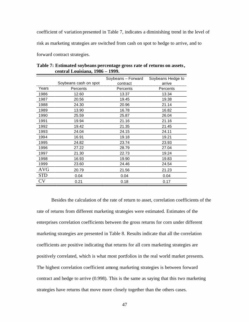
47
coefficient of variation presented in Table 7, indicates a diminishing trend in the level of
risk as marketing strategies are switched from cash on spot to hedge to arrive, and to
forward contract strategies.
Table 7: Estimated soybeans percentage gross rate of returns on assets , central Louisiana, 1986 – 1999.
Soybeans cash on spot
Soybeans – Forward contract
Soybeans Hedge to arrive
Years Percents Percents Percents 1986 12.60 13.37 13.34 1987 20.56 19.45 19.38 1988 24.30 20.96 21.14 1989 13.90 16.78 16.82 1990 25.59 25.87 26.04 1991 19.94 21.16 21.16 1992 19.42 21.35 21.45 1993 24.04 24.15 24.11 1994 16.91 19.18 19.21 1995 24.82 23.74 23.93 1996 27.22 28.79 27.04 1997 21.30 22.73 19.24 1998 16.93 19.90 19.83 1999 23.60 24.46 24.54 AVG 20.79 21.56 21.23 STD 0.04 0.04 0.04 CV 0.21 0.18 0.17
Besides the calculation of the rate of return to asset, correlation coefficients of the
rate of returns from different marketing strategies were estimated. Estimates of the
enterprises correlation coefficients between the gross returns for corn under different
marketing strategies are presented in Table 8. Results indicate that all the correlation
coefficients are positive indicating that returns for all corn marketing strategies are
positively correlated, which is what most portfolios in the real world market presents.
The highest correlation coefficient among marketing strategies is between forward
contract and hedge to arrive (0.998). This is the same as saying that this two marketing
strategies have returns that move more closely together than the others cases.

48
Table 8:Estimated relevant marketing strategies correlation coefficients for Corn, central Louisiana, 1986 – 1999.
Corn\Corn Cash on spot Forward contract Hedge to arrive
Cash on spot 1 0.886 0.889
Forward contract 0.886 1 0.998
Hedge to arrive 0.889 0.998 1
Estimates of the enterprises correlation coefficients between the gross returns for
soybean under different marketing strategies are presented in Table 12. As it is to expect
in most of the real life portfolios, results here indicate that all the correlation coefficients
are positive, which indicates that returns for the entire soybean x soybean enterprise
combination to move positively together. The highest correlation coefficient in this
scenario is the hedge to arrive x forward with a correlation coefficient of 0.964.
Table 9: Estimated relevant marketing strategies correlation coefficients for soybean, central Louisiana, 1986 – 1999.
Soybean\Soybean Cash on spot Forward contract Hedge to arrive
Cash on spot 1 0.924 0.916
Forward contract 0.924 1 0.964
Hedge to arrive 0.916 0.964 1
Cross correlation coefficients between the gross returns from corn and soybean
under different marketing strategies are presented in Table 10. Results indicate that all the
correlation coefficients are positive, meaning that returns for all the corn x soybean
enterprise combination move positively together. The highest correlation coefficient in

49
this scenario is the case corn cash on spot X soybean forward contract with a correlation
coefficient of 0.724.
Table 10: Estimated relevant marketing strategy correlation coefficient for corn-soybeans cross combinations , central Louisiana, 1986 – 1999.
Corn\Soybean Cash on spot Forward contract Hedge to arrive
Cash on spot 0.702 0.724 0.659
Forward contract 0.373 0.512 0.424
Hedge to arrive 0.382 0.528 0.437
The tables of the correlation coefficients show that all the combinations of the marketing
strategies are positively correlated. This means that there is not a unique combination of
marketing strategy in which the risk is completely eliminated. As a result, the study will
work on choosing the combinations of marketing strategies that minimizes the level of
income risk.
Marketing Strategies Portfolio
One of the main objectives of the present study is to find the connection between
marketing strategies decisions and farm’s financial situation. Another objective is to
develop a modeling procedure that links marketing and production decisions. The
approach used for this purpose is the safety first decision criterion. The safety first
decision criterion is used to build an objective function to be run in nonlinear
programming model so that optimal marketing strategies can be estimated. The result
from such non linear programming framework is presented in Table 11.
Optimal marketing strategy for corn and soybeans are presented in Table 11. This
optimal marketing strategy was estimated using the gross rate of return data. Because

50
forward contract marketing strategy and hedge to arrive marketing strategies involve
contracting production for future delivery, the study assumed that the farmers would not
be willing to contract all of the production prior to the harvest date, because there is
production risk that needs to be accounted for. So the restriction on quantity of
production for contract marketing strategy was imposed. The restriction would limit
contracting to the minimum level of production that was observed in the data series time
period. The results from the non linear model show that the optimal marketing strategy
for corn involves 24% cash on spot marketing strategy, 54% forward contract marketing
strategy, and 22% hedge to arrive marketing strategy. For the soybean case, the optimal
marketing strategy given by he non linear program model involves 37% cash on spot
marketing strategy, 30% forward contract marketing strategy, and 33% hedge to arrive
marketing strategy.
Table 11: Estimated optimal marketing strategy portfolio, central Louisiana corn-soybean farm, 1986 – 1999.
Items Corn Soybeans
Cash Market (%)
24
37
Forward Contract (%)
54
30
Hedge to Arrive (%)
22
33
With these proportions estimated, the study could estimate the optimal marketing
strategy portfolio rate of returns. As mentioned before, the study assumed a $1,089.00 per

51
acre farm in assets. So the gross returns from each marketing strategy were also estimated
on percentage terms. The returns of the portfolio are just the weighted average of the
returns from each marketing strategy. The weights are just the proportion by which each
strategy participates in the portfolio. In this study the weights are the ones given by the
non linear programming procedure. So the rates of returns for each marketing strategy
scenario were calculated and are shown in Table 12.
Data from Table 12 shows gross returns for a $1,089/acre in farm assets. These
gross returns differ from the ones previously presented because they represent gross
returns from a farm applying the optimal marketing strategy for corn and soybean
portfolio. The mean return for the optimal marketing strategy for corn is $336.26/acre
and the standard deviation is 74.92. The mean return for the optimal marketing strategy
for soybean is $230.54/acre and the standard deviation is 42.97.
The optimal marketing strategy gross returns are better appreciated when compared with
the traditional cash on spot strategy gross returns. Table13 presents percentage gross rate
of return to asset for corn and soybean farm under traditional cash on spot strategy and
under the optimal marketing strategy for both cash and optimal marketing strategies.
From Table 13, it can be seen that mean rate of return to asset from the optimal
marketing strategy is higher than the returns from the traditional cash on spot strategy for
both corn and soybean. The percentage mean rate of return to asset for cash on spot
strategy for corn is 29.46 and the percentage mean rate of return for the optimal
marketing strategy also for corn is 30.88. The percentage mean rate of return to asset for
cash on spot strategy for soybean is 20.79 and the percentage mean rate of return for the
optimal marketing strategy also for soybean is 21.17.

52
Table 12: Estimated optimal marketing strategy gross return ($/acre), percentage return and distributions, central Louisiana corn-soybean farm, 1986 – 1999.
Years Corn
Optimal marketing strategy1
Soybeans
Optimal marketing strategy2
Gross Return Percent Gross Return Percent
1986 337.8638 0.310251 142.3605 0.130726 1987 311.495 0.286038 216.0465 0.19839 1988 280.5013 0.257577 242.3527 0.222546 1989 239.9682 0.220357 171.2721 0.157275 1990 416.436 0.382402 281.197 0.258216 1991 288.392 0.264823 225.4892 0.207061 1992 417.8589 0.383709 225.0672 0.206673 1993 263.0111 0.241516 262.4073 0.240962 1994 330.8153 0.303779 199.8752 0.18354 1995 327.5083 0.300742 263.5802 0.242039 1996 519.2968 0.476857 300.9564 0.27636 1997 364.4294 0.334646 229.3314 0.210589 1998 267.1043 0.245275 204.4799 0.187768 1999 342.9884 0.314957 263.1278 0.241623 MEAN 336.2621 0.308781 230.5388 0.211698 STD 74.92064 0.068798 42.97409 0.039462 CV 0.222804 0.222804 0.186407 0.186407
1- Rates of return for the optimal marketing strategy for corn are the weighted average of gross rate of return. The weights are the optimal marketing strategy proportions given by the nonlinear programming modeling procedure (24%cash on spot marketing strategy, 54%forward contract, and 22% hedge to arrive marketing strategy).
2- Rates of return for the optimal marketing strategy for soybean are the weighted average of gross rate of return. The weights are the optimal marketing strategy proportions given by the nonlinear programming modeling procedure (37% cash on spot strategy, 30% forward contract, and 33% forward contract marketing strategy).
The gross returns for the marketing strategy scenarios lead the study to the
calculation of net returns. For that, the study assumed levels of variable costs and capital
depreciation for an average 1,000 acre farm using as base the enterprise budget data. This
data were applied to the already estimated gross returns, and allowed for the estimation of
net returns presented in Table 14.
The values presented in Table 14 show the percentage amount by which mean net
rate of return to asset increase when there is a switch from cash on spot strategy to the
optimal marketing strategy. In the case of corn, the percentage mean net rate of return to

53
Table 13: Estimated gross rate of return to asset for corn and soybean farm under traditional cash on spot marketing strategy, and under optimal marketing strategy scenarios, central Louisiana, 1986 – 1999.
Item Cash on spot strategy
Optimal marketing strategy
Corn
Soybean Corn Soybean
Mean Rate of Return to Assets, (%)
29.46
20.79
30.88
21.17
Standard Deviation
6.73
4.46
6.88
3.95
Coefficient of Variation
0.23
0.22
0.22
0.19
Table 14: Estimated net rate of return to asset distribution for cash and optimal marketing portfolio scenario, central Louisiana, corn-soybean farm, 1986 – 1999.
Item Cash on spot strategy Optimal marketing strategy
Corn Soybean Corn Soybean
Mean Rate of Return to Assets (%) 8.87 8.21 10.28 8.58
Standard Deviation (%) 6.73 4.19 6.88 3.95
Coefficient of Variation 0.76 0.51 0.67 0.46
asset increases from 8.87 for cash on spot strategy to 10.28 for optimal marketing
strategy. In the Soybean case there is also an increases in the percentage mean net rate of
return to asset when the marketing strategy is switched from cash on spot to the optimal
marketing strategy. The percentages mean net rate of return to asset increases from 8.21

54
to 8.58. It is good to remember that the values in Table 14 are percentage of a $1,089 per
acre asset, so one percentage increase is a considerable amount of dollars per acre in
gains.
The use of Roy’s safety first criterion and the non linear SAS procedure allowed
for the estimation of optimal marketing strategy, which allowed for the estimation of
gross and net rate of return to asset for the marketing strategies. But the model that links
marketing and production decision is not yet completely estimated. For that to be
accomplished, it is necessary to estimate the production portfolio.
Production Portfolio
In order for the marketing strategies to work, crop production has to be arranged
to meet the marketing requirements. The study assumes that in the production process,
the producers maximize the probability of covering overhead costs, interest, income taxes
and family living expenses. So the amount of commodities to be produced to satisfy the
marketing strategies quantities and to cover all these costs is estimated from the safety
first model. Specifically, the model is estimated by a non linear programming algorithm
and the equation 15 (the objective function for the production portfolio).
It is important to mention that the optimal marketing strategy scenario and the
traditional cash on spot scenario have already been estimated. So the estimation of the
optimal production portfolio for both marketing strategies scenarios is the next step of the
estimation process.
The other aspect that is also important to mention, is that the estimation of the
optimal marketing strategies considered restrictions that allow the farmers a room of
safety in production for the contract requirements that are implied on forward contract

55
and hedge to arrive marketing strategies. The production portfolio that will satisfy the
already estimated marketing strategies and the previously mentioned costs are presented
in Table 15.
Table 15 presents the optimal production portfolio. They were estimated using a
nonlinear programming procedure so that they could satisfy the marketing strategies
already estimated. Data on Table 15 tells that after taking in account all the already
mentioned relevant costs of production and the marketing strategies to be satisfied, the
percentage of corn to be produced for cash marketing scenario is 39%, and for optimal
marketing strategy is 52%. The amount of soybean for cash on spot is 61%, and for the
optimal marketing strategy is 48%.
Table 15: Estimated optimal production portfolio, central Louisiana corn-soybean farm, 1986 – 1999.
Item Corn (%) Soybean (%)
Cash on spot strategy 39 61
Optimal marketing strategy 52 48
Given these production rules the study can calculate the returns these productions can
generate and the risk associated with these returns. For that the study uses the formula of
the rate of return of a portfolio as well as the standard deviation of a portfolio formula. So
the study presents the optimal production portfolio and the standard deviations they infer
in the figures 6 and 7, for both marketing strategies scenarios respectively.
Figures 6 and 7 show the optimal production portfolio under the optimal
marketing strategy and under the cash on spot strategy. The nonlinear programming that
generated this result was the safety first model, which was designed to maximize the

56
probability of covering overhead costs, income taxes, and family living expenses
(equation 15). Figure 6 shows the percentage rate of return to asset generated under the
optimal production portfolio under the cash on spot marketing strategy. The production
portfolio result generated by the non linear program model includes 39% corn production
and 61%soybean production, and the mean rate of return to asset associated with that
production portfolio is 8.47%.
Figure 7 shows the percentage rate of return to asset and the standard deviation
generated under the optimal production portfolio and under the optimal marketing
strategy. The production portfolio result generated by the non linear program model
includes 52% corn production and 48% soybean production, and the mean rate of return
to asset associated with that production portfolio is 9.47%.
A comparison of the optimal production portfolio and cash on spot production
portfolio is presented in the Table 16. Data from the Table 16 shows that returns to asset
increase when marketing strategy is switched from the traditional cash on sport marketing
strategy to the optimal marketing strategy. The mean rate of return to asset of the
portfolio increases from 8.47% to 9.47% for respectively cash on spot strategy and
optimal marketing strategy. The level of risk associated with the generation of the rates of
return to asset for the marketing strategies is higher for the traditional cash on spot
marketing strategy than for the optimal marketing strategy (CV = 0.58 for cash on spot
marketing strategy and CV = 0.51 for the optimal marketing strategy).

57
Figure 6. Optimal production portfolio, under cash marketing strategy, central Louisiana corn-soybean farm, 1986-1999.
Figure 7. Optimal production portfolio under optimal marketing strategy,
central Louisiana corn-soybean farm, 1986-1999
0.07
0.075
0.08
0.085
0.09
0.095
0 0.02 0.04 0.06 0.08
Standard Deviation
Ret
urn
Optimal Portfolio 39% Corn 61% Soybean
0.07
0.075
0.08
0.085
0.09
0.095
0.1
0.105
0.11
0 0.02 0.04 0.06 0.08
Standard Deviation
Ret
urn
Optimal Portfolio Corn: 46 % Soybeans: 54 %

58
Table 16: Estimated production portfolio statistics, central Louisiana corn-soybean farm, 1986 -1999.
Production Portfolio Statistics Cash Optimal
Mean rate of return to assets (r) (%) 8.47 9.47
Standard deviation of rate of return to assets (%) 5.24 4.84
Coefficient of variation 0.58 0.51
Sensitivity Analysis
In the process of estimation of the optimal marketing strategy, assumptions about
the standard deviation and the level of variable cost of production were made. This fact is
of concern when some one wants to know what will happen if the assumptions in the
model were not exactly satisfied. This concern demands for a sensitivity analysis test for
the model. The results of the sensitivity analysis made on the model are presented next.
Table 17 present Sensitivity analysis results estimated for optimal marketing
strategy in a scenario of increasing variable costs for corn. In general results indicate that
as variable costs are increased in the model the optimal marketing strategy for corn
changes. The proportion of corn for cash on spot marketing strategy stays the same as if
the variable costs were not increased (24%). The proportion of corn for forward contract
marketing strategy decreases from 54% to 49% when variable costs are increases by
25%; decreases from 54% to 25% when variable costs increases by 50 %, from 54% to
0% when variable costs are increased by 100%. So as variable costs increases in the
model forward contract marketing strategy becomes less and less suitable for corn.
For hedge to arrive marketing strategy, results indicates that as variable costs
increases in the model, the percentage of corn for hedge to arrive increases from 22% to
27% when variable costs are increased by 25%, from 22% to 51% when variable costs

59
increases by 50%; and when variable costs increases by 100%, the amount of corn for
hedge to arrive increases from 22% to 76%. So as variable costs increases in the model
hedge to arrive becomes more suitable marketing strategy for corn
Table 17: Sensitivity analysis results estimated for optimal marketing strategy in a scenario of increasing variable costs for corn production, central Louisiana corn-soybean farm, 1986 -1999.
Item Normal case Variable cost
up by 25%
Variable cost
up by 50%
Variable cost
up by 100 %
Cash on spot (%) 24 24 24 24
Forward contract (%) 54 49 25 0
Hedge to arrive (%) 22 27 51 76
Table 18 present Sensitivity analysis results estimated for optimal marketing
strategy in a scenario of decreasing variable costs for corn. In general results indicate that
as variable costs are reduced in the model, optimal marketing strategy for corn changes.
The proportion of corn for cash on spot marketing strategy increases as variable costs
decreases. When variable cost decreases by 25% the proportion of corn for cash in spot
marketing strategy increases from 24% to 31%; when variable costs decreases by 50%
the corn for cash marketing strategy increases from 24% to 38%, and from 24% to 46%
when variable costs decreases by 100%. So as variable cost increases in the model cash
on spot marketing strategy becomes more suitable marketing strategy for corn.
The proportion of corn to be allocated for forward contract marketing strategy
decreases from 54% to 53% when variable costs are decreases by 25%; When variable
costs decreases by 50 %, the amount of corn for forward contract decreases from 54% to
51%. And the amount of corn for forward contract decreases from 54% to 48% when

60
variable costs decreases by 100%. So forward contract marketing strategy becomes less
attractive marketing strategy for corn when variable costs decreases.
For hedge to arrive marketing strategy, results indicate that as variable costs
decreases in the model, the percentage of corn for hedge to arrive also decreases from
22% to 16% when variable costs are decreased by 25%, from 22% to 11% when variable
costs decreases by 50%; and when variable costs decreases by 100%, the amount of corn
for hedge to arrive decreases from 22% to 06%. So hedge to arrive becomes less
attractive marketing strategy for corn when variable costs are decreasing.
Table 18: Sensitivity analysis results estimated for optimal marketing strategy in a scenario of decreasing variable costs for corn production, central Louisiana corn-soybean farm, 1986 -1999.
Item Normal case Variable Cost
down by 25%
Variable cost
down by 50%
Variable cost
down by 100%
Cash on spot (%) 24 31 38 46
Forward contract (%) 54 53 51 48
Hedge to arrive (%) 22 16 11 06
Table 19 present Sensitivity analysis results estimated for optimal marketing
strategy in a scenario of increasing standard deviation for corn. In general results indicate
that as standard deviation is increased in the model the optimal marketing strategy for
corn does not change. In this model the standard deviation was increased by 25%, 50%
and 100%. The model was run three times. On each time, the standard deviation was
changed to be the new level. The results were compared to the original case. For the
present case, every time the standard deviation was changed in the model, the results
remained the same as if nothing changed in the model.

61
Table 19: Sensitivity analysis results estimated for optimal marketing strategy in a scenario of increasing standard deviation for corn production, central Louisiana corn-soybean farm, 1986 -1999.
Item Normal case STDV up by 25% STDV up by 50% STDV up by
100%
Cash on spot (%) 24 24 24 24
Forward contract (%) 54 54 54 54
Hedge to arrive (%) 22 22 22 22
Table 20 present Sensitivity analysis results estimated for optimal marketing
strategy in a scenario of decreasing standard deviation for corn. In general results indicate
that as standard deviation is decreased in the model the optimal marketing strategy for
corn does not change. In this model the standard deviation was decreased by 25%, 50%
and 99%.
Table 20: Sensitivity analysis results estimated for optimal marketing strategy in a scenario of decreasing standard deviation for corn production, central Louisiana corn-soybean farm, 1986 -1999.
Item Normal case STDV down by
25%
STDV down by
50%
STDV down by
99%
Cash on spot (%) 24 24 24 24
Forward contract (%) 54 54 54 54
Hedge to arrive (%) 22 22 22 22
Table 21 present Sensitivity analysis results estimated for optimal marketing
strategy in a scenario of increasing variable costs for soybean. In general results indicate
that as variable costs are increased in the model, optimal marketing strategy for soybean

62
changes. Although the proportion of soybean for cash on spot marketing strategy is
unchanged, the proportion of soybean for forward contract marketing strategy increases
from 30% to 31% when variable costs increases by 25% and 50%.And the amount of
soybean for forward contract increases from 30% to 36% when variable costs increases
by 100%. So as variable costs are increased in the model, forward contract marketing
strategy becomes more suitable marketing strategy for soybean.
For hedge to arrive marketing strategy, results indicates that as variable costs
increases in the model, the percentage of soybean for hedge to arrive decreases from 33%
to 32% when variable costs increased by 25% and 50%, from 33% to 27% when variable
costs increases by 100%. So as variable costs increases in the model, hedge to arrive
becomes less suitable marketing strategy for soybean.
Table 21: Sensitivity analysis results estimated for optimal marketing strategy in a scenario of increasing variable costs for soybean production, central Louisiana corn-soybean farm, 1986 -1999.
Item Normal case Variable Cost up
by 25%
Variable cost up
by 50%
Variable cost up
by 100%
Cash on spot (%) 37 37 37 37
Forward contract (%) 30 31 31 36
Hedge to arrive (%) 33 32 32 27
Table 22 present Sensitivity analysis results estimated for optimal marketing
strategy in a scenario of decreasing variable costs for soybean. In general results indicate
that as variable costs decreases in the model the optimal marketing strategy for soybean
are unchanged. This means that the model that generated the optimal marketing results
for soybean is insensitive for decreasing in variable cost. So as variable costs are

63
decreased by 25%, 50%, and 100%, the proportion of soybean for each marketing
strategies (cash on spot , forward contract, and hedge to arrive) remains the same as the
ones that were in use for the normal case (37% cash on spot marketing strategy, 30%
forward contract marketing strategy, and 33% hedge to arrive marketing strategy).
Table 22: Sensitivity analysis results estimated for optimal marketing strategy in a scenario of decreasing variable costs for soybean production, central Louisiana corn-soybean farm, 1986 -1999.
Item Normal case Variable Cost
down by 25%
Variable cost
down by 50%
Variable cost
down by 100%
Cash on spot (%) 37 37 37 37
Forward contract (%) 30 30 30 30
Hedge to arrive (%) 33 33 33 33
Table 23 present Sensitivity analysis results estimated for optimal marketing
strategy in a scenario of increasing standard deviation for corn. In general results indicate
that as standard deviation increases in the model the optimal marketing strategy for
soybean does not change. In this model the standard deviation was increased by 25%,
50%, and 100%.
Table 23: Sensitivity analysis results estimated for optimal marketing strategy in a scenario of increasing standard deviation for soybean production, central Louisiana corn-soybean farm, 1986 -1999.
Item Normal case STDV up by 25% STDV up by
50%
STDV up by
100%
Cash on spot (%) 37 37 37 37
Forward contract (%) 30 30 30 30
Hedge to arrive (%) 33 33 33 33

64
Table 24 present Sensitivity analysis results estimated for optimal marketing
strategy in a scenario of decreasing standard deviation for soybean. In general results
indicate that as standard deviation is decreased in the model the optimal marketing
strategy for soybean does not change. In this model the standard deviation was decreased
by 25%, 50% and 99%.
Table 24: Sensitivity analysis results estimated for optimal marketing strategy in a scenario of decreasing standard deviation for soybean production, central Louisiana corn-soybean farm, 1986 -1999.
Item Normal case STDV down by
25%
STDV down by
50%
STDV down by
100%
Cash on spot (%) 37 37 37 37
Forward contract (%) 30 30 30 30
Hedge to arrive (%) 33 33 33 33
Financial Implications
Different marketing strategy scenarios are expected to yield different financial
performances. After the estimation of rates of returns to asset, the financial model was
used to estimate the financial implications of the marketing strategies. The financial
model is made of three equations, the equation estimating the rate of return to equity, the
equation estimating the required rate of equity formation, and the equation estimating the
lower confidence interval of the rate of return to equity.
The computation of the financial variables for the present study (profitability,
risk, liquidity, and debt repayment capacity) requires that the study makes assumptions
about financial parameters so that calculations can be carried out. Table 25 presents the
assumptions.

65
Data in Table 25 shows the parameters needed for the computation of financial
variables. It is important to mention that all the assumed parameters are chosen to be
equal for both marketing strategies, for example the farm size was assumed to be 1,000
acres for both marketing strategies scenarios, the debt to equity and all other financial
parameters are also assumed to be equal for both marketing strategies scenarios and are
expressed as a proportion or percentage of the farm’s equity.
The financial model allowed for the calculations of the financial results presented
in Tables 26, and 27. Table 26 shows the debt to equity ratios, the rate of return to equity
(Re), the required rate of equity formation (R’), the standard deviation of the rate of
return to equity (STDEV), the lower side interval of the rate of return to equity capital
(RL), the t-values associated with rate of return to equity, the probability of financial
success, the levels of profitability, risk (measured by the coefficient of variation of return
to equity), and liquidity. The financial parameters in Table 26 were estimated taking in
consideration that the farmer needs to meet financial commitments in nine out of 10 years
(risk case scenario). Table 26 presents results for the financial model under the cash on
spot marketing strategy scenario, and Table 27 presents results for the optimal marketing
strategy scenario. Estimates presented in Table 26 indicate that the maximum debt
repayment capacity under risky scenario occurs at a debt to equity level of 0.514646. At
that level, the required rate of return (R’) equals the lower side interval of the rate of
return to equity capital (RL) at the level 0.46575 percent. At this return level, the
probability of meeting all financial commitments is 0.90. However the actual ratio of debt
to equity on the farm is 0.633074. The probability of meeting all financial commitments
under this scenario is 0.71733, or approximately seven out of 10 years.

66
Table 25. Capital structure, financial parameters, and financial performance estimates, central Louisiana corn-soybean farm, 1999.
Item Marketing Scenarios
Cash Optimal
Farm size (acres) 1,000 1,000
Capital structure
Debt ($) 422,159 422,159
Equity ($) 666,841 666,841
Financial parameters
Actual debt/equity (d/e) 0.633 0.633
External income (e) (%) 6.000 6.000
Operating interest (s) (%) 0.500 0.500
Interest rate on capital asset debt (i) (%) 9.000 9.000
Overhead expenses (o) (%) 2.470 2.470
Average income taxes (t) (%) 20.000 20.000
Withdrawals for consumption (w) (%) 2.296 2.296
The level of profitability is estimated as the mean rate of return to equity. Under
the cash on spot marketing strategy scenario the profitability is estimated at 6.69%. The
level of risk is measured by the coefficient of variation of the rate of return to equity. For
the cash on spot marketing strategy it is estimated at 1.01. The level of liquidity is
estimated as the sum of profitability and credit reserve (difference between maximum and
actual debt), and for the cash on spot marketing strategy it is estimated at negative 6.69.
This value is the same as the value of mean rate of return to equity or profitability. The
value of the credit reserve for the cash on spot marketing strategy is assumed to be zero,
instead of a negative value, that the estimation from the data on table 26 would suggest. It
is because the concept of a zero credit reserve does not make sense.

67
Table 26.Financial parameters, and financial performance estimates for cash on
spot marketing strategy, central Louisiana corn-soybean farm, 1986-1999.
Cash on spot Debt/Equity Re (%) R' (%) STDEV RL (%) t-VALUE Probability
0 0.069034 0 0.038299 0.055216 6.744335 0.999993 0.1 0.068738 0.00905 0.042129 0.053537 5.301107 0.999928 0.2 0.068441 0.0181 0.045959 0.051859 4.098417 0.999372 0.25 0.068293 0.022625 0.047874 0.05102 3.569234 0.998286 0.3 0.068145 0.02715 0.049789 0.050181 3.080757 0.995617 0.4 0.067848 0.0362 0.053619 0.048502 2.208476 0.977111 0.5 0.067551 0.04525 0.057449 0.046824 1.4525 0.914965
0.514646 0.067508 0.046575 0.05801 0.046575 1.350162 0.899999 0.6 0.067255 0.0543 0.061279 0.045145 0.79102 0.778438
0.633074 0.067157 0.057293 0.062545 0.04459 0.590071 0.71737 0.7 0.066958 0.06335 0.065109 0.043467 0.207362 0.58053 0.8 0.066662 0.0724 0.068939 0.041789 -0.31145 0.6198 0.9 0.066365 0.08145 0.072769 0.04011 -0.77564 0.77408 1 0.066069 0.0905 0.076598 0.038432 -1.19342 0.872985
1.1 0.065772 0.09955 0.080428 0.036753 -1.57141 0.92995 1.2 0.065475 0.1086 0.084258 0.035075 -1.91503 0.961125 1.3 0.065179 0.11765 0.088088 0.033396 -2.22878 0.97795 1.4 0.064882 0.1267 0.091918 0.031718 -2.51638 0.98711 1.5 0.064586 0.13575 0.095748 0.03004 -2.78097 0.992206
Financial estimates for the optimal marketing scenario are presented in Table 27.
Table 27 shows the debt to equity ratios, the rate of return to equity (Re), the required
rate of equity formation (R’), the standard deviation of the rate of return to equity
(STDEV), the lower side interval of the rate of return to equity capital (RL), the t-values
associated with the rate of return to equity, the probability of financial success, the levels
of profitability, risk (CV), and liquidity. The financial parameters in Table 27 were
estimated taking in consideration that farmer needs to meet financial commitments in
nine out of 10 years (risk case scenario).
Estimates presented in Table 27 indicate that the maximum debt repayment
capacity under risky scenarios for the optimal marketing strategy occurs at a debt to
equity ratio of 0.640306. At that level, the required rate of return (R’) equals the lower

68
side interval of the rate of return to equity capital (RL) at the return level of 0.05795
percent. At this return level, the probability of meeting all financial commitments is
approximately 0.90 (nine out of 10 years). However the actual level of debt on the farm is
0.633074. The probability of meeting all financial commitments under this scenario is
approximately 0.91 or approximately nine of 10 years. So, with the introduction of
optimal marketing strategy the maximum debt repayment capacity improves from a debt
to equity ratio of 0.514646 to 0.640306 and the probability of repaying the actual level of
debt improves to 0.90 from 0.71 in the cash on spot scenario.
As in the case of cash on spot marketing strategy, the level of profitability is
estimated as percentage of mean rate of return to equity. Under the optimal marketing
strategy scenario the profitability is estimated at 8.13%. The level of risk is measured by
the coefficient of variation of the rate of return to equity and for the optimal marketing
strategy it is estimated at 0.87. The level of liquidity is estimated as the sum of
profitability and credit reserve (difference between maximum and actual debt), and for
the cash on spot marketing strategy it is estimated at 8.86%.
Comparison of financial parameter estimates between cash on spot marketing strategy
and optimal marketing strategy scenarios are presented in Table 28. Table 28 presents
actual debt to equity ratio, maximum debt to equity repayment capacity, probability of
repaying the actual level of debt, probability of repaying the maximum level of debt, the
levels of profitability, risk, and liquidity for both cash and optimal marketing strategy
scenarios. Results presented in Table 28 show that optimal marketing strategy has higher
maximum level of debt to equity, regardless of the fact that both marketing strategies
started with the same actual level of debt to equity ratio.

69
Table 27. Financial parameters, and financial performance estimates for optimal marketing strategy, central Louisiana corn-soybean farm, 1986-1999.
Optimal marketing Strategy Debt/Equity Re (%) R' (%) RL (%) STDEV t-VALUE Probability
0 0.077046 0 0.063433 0.037352 7.704288 0.999998 0.1 0.077551 0.00905 0.062576 0.041088 6.224476 0.999985 0.2 0.078055 0.0181 0.061719 0.044823 4.9913 0.999877
0.25 0.078308 0.022625 0.061291 0.04669 4.448702 0.999672 0.3 0.07856 0.02715 0.060863 0.048558 3.947843 0.999166 0.4 0.079065 0.0362 0.060006 0.052293 3.053451 0.995381 0.5 0.079569 0.04525 0.059149 0.056029 2.278312 0.979878 0.6 0.080074 0.0543 0.058293 0.059764 1.600065 0.933203
0.633074 0.080241 0.057293 0.058009 0.060999 1.394021 0.906659 0.640306 0.080277 0.05795 0.05795 0.061269 1.350071 0.899984
0.7 0.080579 0.06335 0.057436 0.063499 1.001611 0.832594 0.8 0.081083 0.0724 0.056579 0.067234 0.469653 0.676808 0.9 0.081588 0.08145 0.055722 0.07097 -0.00631 0.502469 1 0.082092 0.0905 0.054866 0.074705 -0.43468 0.664537
1.1 0.082597 0.09955 0.054009 0.07844 -0.82225 0.787119 1.2 0.083102 0.1086 0.053152 0.082175 -1.17458 0.869385 1.3 0.083606 0.11765 0.052296 0.08591 -1.49628 0.92077 1.4 0.084111 0.1267 0.051439 0.089646 -1.79117 0.951718 1.5 0.084616 0.13575 0.050582 0.093381 -2.06247 0.970131
The probability of repaying the actual level of debt is higher for the optimal
marketing strategy scenario than for the cash on spot marketing strategy scenario.
Although the probability of repaying the maximum level of debt that each marketing
strategy can hold is similar for both marketing strategy scenarios (90%), the maximum
debt to equity ratio is higher for the optimal marketing strategy scenario (0.64 ) than for
the cash on spot marketing strategy scenario (0.51). The level of profitability is higher for
the optimal marketing strategy scenario (8.13%) than for the cash on spot marketing
strategy scenario (6.69%). Optimal marketing strategy scenario presents lower level of
risk (coefficient of variation of return to equity) than the cash on spot marketing strategy
scenario (0.86 against 1.001 respectively). The level of liquidity is higher for the case of

70
optimal marketing strategy (8.86%) than for the cash on spot marketing strategy case
(6.69%).
Table 28: Comparison of financial performances between cash on spot marketing strategy and optimal marketing strategy, central Louisiana 1986 - 1999
Financial Performance Cash Optimal
Actual debt to equity ratio 0.63 0.63
Maximum debt repayment capacity (d/e) 0.51 0.64
Probability of meeting financial commitments for actual debt (%) 71 90
Probability of meeting financial commitments for maximum debt (%) 90 90
Profitability (%) 6.69 8.13
Risk measured by coefficient of Variation 1.01 0.87
Liquidity (%) 6.69 8.86
Graphical illustrations of the process of estimation of maximum debt capacity are
presented in Figure 8 and 9. Figure 8 shows the line representing the required rate of
equity formation and the rate of return to equity from both marketing strategies under
certainty conditions. Results in the Figure 8 show that under certainty conditions, the
return to equity from the optimal marketing strategy scenario is higher than the returns to
equity from the cash on spot strategy. The maximum debt to equity ratio that a marketing
scenario can absorb is estimated by the crossing point between the line representing the
required rate of equity formation and the line representing the rate of return to equity.
Figure 9 shows the line representing the required rate of equity formation and the rate
of return to equity from both marketing strategies under risky conditions. Results in
Figure 9 show that under risky conditions, the returns to equity from the optimal
marketing strategy scenario are higher than the returns to equity from the cash on spot
marketing strategy. As in the certainty case the maximum debt capacity is estimated

71
the lines representing the rate of return to equity (for both marketing strategies)
faces the same line of required rate of equity formation, the scenarios that shows higher
level of return to equity ends up having higher level of maximum debt repayment
capacity. Actual debt is below maximum debt for both marketing scenarios.
Contra
Figure 8.Estimated debt repayment capacity under certainty conditions, cash and optimal marketing scenarios, Louisiana corn-soybean farm, 1986-1999.
by the intersection of the line representing the required rate of equity formation and the
line representing the rate of return to equity. Since the lines representing the rate of return
to equity (for both marketing strategies) faces the same line of required rate of equity
formation, the scenarios that shows higher level of return to equity ends up having higher
level of maximum debt repayment capacity. For the risky condition case the actual debt is
no longer bellow maximum debt for the cash marketing scenario.
0
2
4
6
8
10
12
14
16
0 0.2 0.4 0.6 0.8 1 1.2 1.4 1.6
Debt to Equity
Per
cent
Ret
urn
Required Equity Formation
Return to Equity with Cash Marketing
Maximum Debt
Maximum Debt
Actual Debt
Return to equity with optimal marketing strategy

72
Figure 9. Estimated debt capacity under risky conditions, cash and optimal marketing scenarios, Louisiana corn-soybean farm, 1986 - 1999.
Figures 8 and 9 illustrates that the maximum debt supported by the optimal
marketing strategy is higher than the maximum debt that the cash on spot strategy can
support. This makes sense, because the return to equity line is higher for the case of
optimal marketing strategy (for certainty and risky case) and face the same level of
required rate of equity formation. The gap between the level of maximum debt and actual
debt tells that the credit reserve is higher for the case of optimal marketing strategy when
compared to the cash on spot strategy (for certainty and risky scenarios).
The financial implications of the marketing strategies on the equity of the
representative farm are summarized in the Figure 10. Figure 10 shows that if the farm
needs to meet financial commitments in nine of 10 years, the optimal marketing strategy
is the one that appears to have better results, since is presents higher profitability when
compared to the cash on spot strategy (8.13 against 6.69 respectively), lower risk (0.87
0
2
4
6
8
10
12
14
16
0 0.5 1 1.5 2
Debt to Equity
Per
cent
Ret
urn
Return to Equity with Optimal Marketing
Required Equity Formation
Return to Equity with Cash Marketing
Actual Debt
Maximum Debt
Maximum Debt

73
against 1.01 respectively), and higher liquidity (8.86 against 6.69 respectively).This is
one more time a confirmation of the advantage of opting for advanced marketing
strategies instead of the traditional cash on spot marketing strategy.
Figure 10. Financial performance measures for cash and optimal marketing strategies, representative farm, central Louisiana, 1986-1999.
0
2
4
6
8
10
Per
cen
t
Cash 6.69 1.01 6.69
Optimal 8.13 0.87 8.86
Profitability (%)
Risk (CV) Liquidity (%)

74
CHAPTER V
SUMMARY AND CONCLUSIONS
Agriculture is inherently risky. Output from the farm in most cases depends on
weather and biological processes over which producers have little control (Fleisher,
1990). Besides the biological and environmental issues surrounding the agriculture
production sector, its structural characteristics are capital intensive where both leasing
and credit are extensively used to acquire resources for production. The agriculture
production sector also operates in an environment of volatile input and output markets,
risky production environment, and policy uncertainties. These factors create a complex,
and risky climate (Barry et al., 1995). The producer is faced with the challenge of
acquiring and combining resources within the firm to increase the welfare of the business
and at the same time protect farmer’s equity within the business. So, income risk in
agriculture is a problem that can not be dismissed. Financial problems in agriculture
became so serious that many farmers started thinking about leaving the farm sector
(Swanberg and Marra, 1987).
Through out the years, farm income risk became a known problem. In fact, for
many years government has been absorbing income risk in agriculture by the mean of
different policy tools such as (direct payment, price support, etc.). In a Nebraska’s
farmer’s survey, Johnson 1996 found that the most common risk management strategy
among farmers was government program participation. However, policy swings from
time to time poses concerns regarding a need for an alternative risk absorbing mechanism
in agriculture. The 1996 farm act and the 2001 farm bill show two different scenarios of
government intervention in agriculture, the first supporting the phasing out of the
75
government intervention and the other supporting the phasing in of the government
intervention in Agriculture. Situations like this make someone ask if there is not out there
any other alternative way for managing income risk beside government intervention. In
fact, all this policy uncertainties indicate that there is a need for farmers, as well as
politicians, and decisions makers, to have a larger range of risk absorbing alternatives.
The literature suggests that in the absence of government programs, a large group
of farmers would increase the use of marketing tools to increase their returns. Barry et al.
argue that marketing alternatives such as cash on spot selling strategy, forward
contracting strategy, and hedge to arrive contracting strategy provide farmers with
methods for risk management.
While it is generally recognized that farmers can use marketing strategies to
manage risk, and that marketing strategies can provide an alternative and meaningful way
of managing income risk in the farm business, there are few studies in the literature about
how these marketing strategies can be effectively applied for farmers to improve their
financial conditions and manage risk. An important question concerns the relationship of
pre-harvest marketing strategies and farmers financial performance. More specifically,
what is the relationship between pre-harvest marketing strategies and financial
performance measures such as farm profits, risk and liquidity?
General Approach
The general objective of this study is to examine the relationship between pre-harvest
marketing strategies and financial performance measures (profit, liquidity, and risk) of a
representative soybean-corn farm in central Louisiana. The specific objectives include the
identification of a representative grain crop farm in central Louisiana; the identification

76
of pre-harvest marketing strategies for the selected grain crops in central Louisiana; the
estimation of the rate of return to asset distributions for the identified pre-harvest
marketing strategies and grain crops in the study area; the development of a modeling
procedure for estimating the relationship between marketing decisions and production
decisions; and the estimation the effect of pre-harvest marketing decisions, on the
financial performance of a representative farm in the target area.
The general approach of the study is to measure financial performance of a
representative soybean-corn farm in the target area in Louisiana under different
marketing scenarios. The study uses a portfolio approach assuming safety first decision
criteria to estimate optimal marketing portfolio and optimal enterprise production
combination. The results are applied with a three equations financial model to estimate
the financial performance (profitability, risk and liquidity) of the marketing strategy for a
representative farm in Louisiana under the optimal marketing strategies and the
traditional cash on spot marketing strategy.
Data and Procedures
The first task was to choose the representative grain crop farm for the study. To
identify a representative grain crop farm in Louisiana, the study reviewed farm budgets,
rural land and survey data, along with data from Louisiana’s Farm Bureau statistics. The
study also used departmental farm survey and farm enterprise budget data. This allowed
for the selection of local, and commodities that would have the necessary level of data for
the estimations. The identification of the pre-harvest marketing strategies for selected
grain crops in the study area, involved interviews with marketing extension specialists

77
and a collection of information from local elevators about the more predominant
marketing strategies in use for the relevant grain crops in Louisiana.
Optimal marketing strategies were estimated by a nonlinear programming
procedure (SAS). The objective function of the non linear programming was estimated by
the application of the Roy’s safety first decision criteria (maximize the probability that
returns on the portfolio is greater than the critical level bellow which returns should not
fall) to the problem at hand. A sensitivity analysis was done to the model estimating the
optimal marketing strategy.
After estimating the optimal marketing strategies the study finds the optimal
production portfolio, which is the one that will satisfy the already found optimal
marketing combination. For that, the study applies the same Roy’s safety first formula to
find an objective function to run the non linear programming SAS software.
Now that the optimal marketing strategies and production combination are
estimated, the study estimates the financial implication of these marketing strategies.
Financial measurements of profitability, liquidity, and debt repayment capacity are
estimated for the two marketing scenarios (cash on spot and optimal marketing strategy)
and applied to a 1,000 acre representative farm. The study assumes a specific amount of
debt and estimate the risk adjusted capacity of repaying the debt in nine out of 10 years.
The profitability associated with each marketing strategy is estimated by using the
financial model, which estimates the rate of return to equity. The level of profitability is
estimated as the mean rate of return to equity for the representative farm. Liquidity is
estimated by adding the profitability to the corresponding credit reserve. Credit reserve is

78
estimated by subtracting actual debt from maximum debt allowed under the
corresponding marketing strategy.
The maximum debt capacity that each marketing strategy can accommodate under
certainty condition is estimated by equalizing the equation of the rate of return to equity
and the equation for the required rate of equity formation. The actual level of debt is
externally given. The risk adjusted level of maximum debt is given by equalizing the
equation of low sided interval of the rate of return to equity and the required rate of
equity formation. The level of risk associated with the use of each marketing strategies
are estimated by the coefficient of variation of rate of return to equity.
Results
Visits with the marketing extension specialist and data collection from the local
elevators suggested that the predominant marketing strategies in use in the target area are
cash on spot marketing strategy, forward contract marketing strategy, and hedge to arrive
marketing strategy. These are the marketing strategies that the literature refers as the ones
having the potential to be used for the purpose of reducing income risk.
Results from the non- linear programming for estimating the optimal marketing
strategy suggest that for corn the optimal marketing strategy would include 24% cash on
spot strategy, 54% forward contract marketing strategy, and 22% hedge to arrive. In the
case of soybean the result from the nonlinear programming suggests that the optimal
marketing strategy would include 37% cash on spot marketing strategy, 30% forward
contract, and 33% hedge to arrive marketing strategy.
The sensitivity analysis done to the model that estimates the optimal marketing
strategy suggests that optimal marketing strategy is insensitive to changes in the standard

79
deviations values used in the model. The proportions of corn and soybean sold in the cash
market appear to be insensitive to increases in the variable costs. When variable costs are
increased in the model, the proportion of hedge to arrive in the model increases for corn
and the proportion of forward contract in the model increases for soybean. When variable
costs are decreased in the model, the proportion of cash on spot marketing strategy
increases in the model for corn.
The optimal production portfolios using Roy’s safety-first model were estimated
for the cash marketing and optimal marketing portfolios. Nonlinear optimization
procedures were also used to estimate optimal production portfolios. Optimal production
portfolios maximize the probability of covering overhead, interest, income tax, and
family living expenses. Comparing the cash on spot strategy production scenario with the
optimal marketing strategy production scenario it can be seen that the production
decisions are different. In the cash on spot production decision the study found that 39%
of corn and 61% of soybean as the recommended amounts. For the optimal marketing
strategy, the nonlinear procedures production portfolio estimates that corn production
increases to 52% and soybean production decreases to 48%. The means return to assets
for the optimal production portfolios are estimated to be 8.47% and 9.47% for cash and
optimal marketing scenarios, respectively.
For estimating the financial implications of adopting the marketing strategies a
1,000 acre farm were selected and several financial parameters were assumed for the
calculation procedures. Results are presented in a way such that cash on spot strategy
scenario is contrasted with the optimal marketing strategy scenario.

80
The actual level of debt is assumed to be $422,159 and the equity is $666,841.
This result gives the actual debt to equity ratio of 0.633 for each marketing scenario.
Financial parameters assumptions are the same for each marketing strategy scenarios;
however, financial performance measures differ by each of the marketing strategies. In
terms of debt repayment capacity, it is assumed in this analysis that the producer wishes
to meet all of the firm’s financial commitments in nine out of ten years. Results indicate
that maximum debt repayment capacity is greater for the optimal marketing scenario than
for the cash marketing scenario. Maximum debt repayment capacity for the optimal
marketing scenario is estimated at a debt to equity ratio of 0.64, whereas for the cash
marketing scenario, it is estimated to be 0.51.
Profitability, risk, and liquidity financial indicators indicate that the optimal
marketing plan is financially better than the cash marketing alternative. In terms of
profitability, the optimal marketing scenario offers a profitability level of 8.13 percent
rate of return to equity, whereas this rate for the cash marketing alternative is 6.69
percent. The optimal marketing strategy is less risky than the cash marketing scenario,
since it presents a lower level of coefficient of variation (0.86 against 1.01 for optimal
and cash on spot marketing strategies scenarios respectively). Liquidity for the farm is
estimated as the sum of the dollar returns to equity capital and the dollar amount of
unused credit expressed in terms of equity. Liquidity is greater for the optimal marketing
scenario than for the cash marketing scenario (8.86 percent versus 6.69 percent).
Limitations of the Study
The present study uses a portfolio approach for estimating the optimal marketing
strategy for achieving the best financial results. The marketing strategies used in the

81
present study were identified from interviews from marketing extension specialists and
elevators working in the area. Future research should attempt to verify pre-harvest
marketing strategy based on farmer’s data.
One of the objectives of this study is to present a modeling procedure linking pre-
harvest marketing strategies to production decision as well as their financial implications.
For that, a quite wide representative data sample would be required. However the local
level data availability was limited so that the study had to work with a limited amount of
yield and price data. Futures research should attempt to test the sensitivity of financial
results to variation of data.
Along with the limitation just described above, regarding the sample size, a
similar argument can be raised concerning the number of crops included in the study.
Since the study has this modeling approach, it would be good to include a considerably
large amount of crops for the study. But since it would be highly time consuming, as well
as it would involve large and complicated levels of calculation the study decided to work
with a “small” amount of crops. For future studies, other crops and situations should be
considered. Also further research should also include the application of the model to
more complex farming situations and marketing strategies.
Another limitation comes from the estimation of financial implications of the
marketing strategies. For the calculations of debt repayment capacity under risky and
certainty, as well as for the calculation of liquidity several assumptions of financial
parameters were made. Parameters such as interest rate, the level of actual debt, the
family withdrawals, and depreciation were assumed to be fixed at a specific level. Future

82
research should consider incorporating variability associated with all the parameters that
were assumed to be fixed into the modeling procedure.
One more limitation of the study comes from the fact that the study uses a parish
level data, and the study results are supposed to be used by farmers. Since parish level
data is aggregate of the farmers data, questions can be raised regarding the variability
involved in applying results obtained using parish level data to a particular farm. But it is
good to mention that the data used in the study was obtained by the Louisiana’s
statisticians using the best sampling and knowledge available and represents in average
the Parish farmer’s data. However it is good to ment ion that if trying to use the results of
this study to a particular farmer, it is better to use the specific farm data.
Conclusions
The present study illustrates how different marketing strategies affect farm
production decisions as well as financial performance. One important financial variable
includes debt carrying capacity for a farming scenario, where debt carrying capacity is
measured by the debt to equity ratio. Results of the analysis indicate that optimal pre-
harvest marketing portfolios have larger estimated debt carrying capacities under
certainty and risky conditions than the traditional cash marketing strategy scenario.
The results also indicate that different pre-harvest marketing strategies result in
different levels of farm risk. The research indicates that marketing the crops at harvest in
the cash market has the highest level of income risk. Whereas, if a portfolio of optimal
pre-harvest marketing strategies are used, the farm is able to meet all of its financial
commitments in nine out of ten years. Consistent with financial literature, empirical
findings here illustrate a direct relationship among farm marketing, production, and

83
financial management processes. The portfolio approach to marketing resulted in
improved financial performance (profits, risk, and liquidity) for the representative farm
over traditional cash marketing methods.
84
REFERENCES
Ahrendsen, B.L. Federal Legislation: “Agricultural Credit Issues and Institutions, “Special report 171, Arkansas Agricultural Experimental Station, University of Arkansas, November 1995.
Barry, Peter J., Ellinger, Paul N., Baker, C. B., Hopkin, John A., “Financial Management in Agriculture.” Interstate Publisher, Inc., Danville, Illinois, 2000. Catlett, Lowell B., Libbin, James D. “Investing in Futures & Options Markets.” Delmar Publisher 1999. Albany, New York. Cotterill, R.W., “Food marketing policy center”., WWW.CWF.UVM.EDU/CRIS.
10/16/2001. Elton, Edwin J., Gruber, Martin J. “Modern Portfolio Theory and Investment Analysis”.
John Wiley & Sons. 1981. Fleisher, Beverly. “Agricultural Risk Management,” Lynne Rienner Publishers, Boukder & London, 1990; Harwood, Joy et al. “Managing Risk in Farming: Concepts, Research, and Analysis.
Market and Trade Economics division and Resource Economics division, Economic Research Service. USDA. Agriculture Economic Report N0 774
Johnson, Bruce. “A Financial Profile of Nebraska Farm Business -1994, “Research
Report. No. 174, Department of Agricultural Economics, University of Nebraska, Lincoln, July1996.
Kahl, K.H.; Miller, S. E., Curtis, C. E. “Marketing Strategies for Managing
Agriculture Income Risk in South Caroline” .WWW.CWF.UVM.EDU/CRIS., 04/04/2001
Koo, Won., Marvin R. Duncan, and Richard D. Taylor. “Analysis of farm financing and
Risk Management for U.S. farmers,” Agricultural Economics Reports No, 399, Department of Agriculture, Agriculture Experiment Station, North Dakota State University, Fargo, North Dakota, July, 1998.
Larson, J. A., “Economic Assessment of Agricultural risk and financial management
Strategies.” CWF.UVM.EDU/CRIS. 01/22/2001 Lewis, C.E.,” Marketing Alaska’s Agricultural and processed seafood products”. 07/08/2001.WWW.CWF.UVM.EDU/CRIS.,01/22/2001. Little, R. D. “Economic Analysis of livestock production, Management, and Marketing
Practices in Mississippi.” CWF.UVM.EDU/CRIS. 04/04/2001

85
Mclemore, D. L., “Evaluation of pricing/ Marketing strategies for Tennessee feeder cattle producers”. CWF.UVM.EDU/CRIS. 01/12/1999. Melichar, Emanuel. “A financial perspective on agriculture,” Federal Reserve Bulletin, Federal Reserve Board, Washington D.C., January 1984. Pindyck, Robert S., and Daniel L. Rubinfeld. “Microeconomics” 5th Edition, Prentice
Hall, Inc., New Jersey, 2001. Qasmi, B. A. “Economic Assessment of grain Marketing Patterns, practices and strategies in South Dakota. CWF.UVM.EDU/CRIS. 03/22/2000 Tiller, K.H. “Tennessee Financial Analyses and Risk management Strategies
(TNFARMS): Farm level Policy Analyses for Tennessee”. WWW.CWF.UVM.EDU/CRIS.08/07/2001
Vandeveer, L. R., Henning, S. A., Kennedy, G. A., Li, C. “Financial implications of a
new farm policy environment,” Journal of Agribusiness 18, 3 (Fall 2000): 237-247).
Vandeveer, L. “Financia l Analysis of a Major Louisiana Farming Situations. CWF.UVM.EDU/CRIS.04/04/2001 Xiao, J. J.; Newman, B. M.; Prochaska, J. M. “Applying the trans-theoretical model of change to financial behavior.

86
VITA
Manuel Duarte Filipe, was born October 16, 1971 in the city of Beira, Province of
Sofala, in Mozambique (south east Africa). In December 1989 he graduated from Samora
Machel Secondary and pre-University school (High school).
In 1990 Manuel Duarte Filipe was awarded a scholarship from the government of
Mozambique and enrolled at the Eduardo Mondlane University to pursue a bachelor of
science degree in agronomy. In 1996 Manuel Duarte Filipe graduated from Eduardo
Mondlane University with a bachelor of Science degree in agronomy. In the same year he
was recruited to work in a World Bank financed project at the Mozambican National
Agronomic Research Institute.
In 1999, Manuel Duarte Filipe was awarded a scholarship by United State Agency
for International Development to pursue a master’s degree in agricultural economics. In
January 2000 he enrolled at the Department of Agricultural Economic at Louisiana State
University in Baton Rouge. Now he is a candidate for a master’s degree in agricultural
economics.
Upon graduation, he plans to continue with his studying plans and pursue a
doctoral degree in agricultural economics. He has been accepted for that program by the
Purdue University in Indiana.