NBER WORKING PAPER SERIES

AN ECONOMETRIC EVALUATION OF COMPETING EXPLANATIONS FOR THEMIDTERM GAP

Brian G. Knight

Working Paper 20311http://www.nber.org/papers/w20311

NATIONAL BUREAU OF ECONOMIC RESEARCH1050 Massachusetts Avenue

Cambridge, MA 02138July 2014

Thanks to Alex Effenberger for research assistance and for help with the literature review section ofthis paper. Thanks to Claire Lim for helpful comments and to seminar and conference participantsat Harvard University, MIT, New York University, Johns Hopkins, Caltech, UC-Berkeley, Wake ForestUniversity, Stanford University, Cornell University, the London School of Economics, UniversityofWarwick, University of Toronto, and the CIRPÉE-UQAM Conference on Political Institutions. Theviews expressed herein are those of the author and do not necessarily reflect the views of the NationalBureau of Economic Research.

NBER working papers are circulated for discussion and comment purposes. They have not been peer-reviewed or been subject to the review by the NBER Board of Directors that accompanies officialNBER publications.

© 2014 by Brian G. Knight. All rights reserved. Short sections of text, not to exceed two paragraphs,may be quoted without explicit permission provided that full credit, including © notice, is given tothe source.

An Econometric Evaluation of Competing Explanations for The Midterm GapBrian G. KnightNBER Working Paper No. 20311July 2014, Revised November 2015JEL No. D7

ABSTRACT

This paper provides a unified theoretical and empirical analysis of three longstanding explanationsfor the consistent loss of support for the President’s party in midterm Congressional elections: (1)a Presidential penalty, defined as a preference for supporting the opposition during midterm years,(2) a surge and decline in voter turnout, and (3) a reversion to the mean in voter ideology. To quantifythe contribution of each of these factors, we build an econometric model in which voters jointly choosewhether or not to participate and which party to support in both House and Presidential elections. Estimatedusing ANES data from both Presidential and midterm years, the model can fully explain the observedmidterm gaps, and counterfactual simulations demonstrate that each factor makes a sizable contributiontowards the midterm gap, with the Presidential penalty playing the largest role.

Brian G. KnightBrown UniversityDepartment of Economics, Box B64 Waterman StreetProvidence, RI 02912and NBERBrian_Knight@brown.edu

1 Introduction

One of the most striking empirical regularities in American politics involves the midterm gap,

under which the President’s party routinely loses seats in Congressional elections held during

midterm years. Since 1876, the President’s party has lost seats in all cases except for 1934, 1998,

and 2002 (Folke and Snyder, 2012). Recent cases with large swings include 1974, when President

Ford’s party lost 48 out of 435 seats in the House and 4 out of 100 seats in the Senate, 1994, when

President Clinton’s party lost 54 seats in the House and 9 seats in the Senate, and 2010, when

President Obama’s party lost 63 seats in the House and 6 seats in the Senate.

There is a long literature in political science developing and testing hypotheses regarding dif-

ferent mechanisms underlying this midterm gap, and this paper addresses three such long-standing

hypothesized mechanisms. First, due to a Presidential penalty, midterm voters, conditional on

participating, may have a preference for the opposition and express this preference in the voting

booth. This preference could reflect, among other factors, a dissatisfaction with the President’s

performance or a preference for divided government. Second, there may be a surge and decline

in voter turnout, with supporters of a strong Presidential candidate energized to participate in the

Presidential year but not turning out to vote in midterm years. Third, there could be a reversion to

the mean in voter ideology, with the President’s party advantaged in Congressional races during

the Presidential year before ideology returns to its normal state in the midterm year.

To quantify the contribution of each of these factors, we build and estimate a statistical model

in which voters jointly choose whether or not to participate and, conditional on participating, which

party to support in both House and Presidential elections. To accommodate the Presidential penalty

hypothesis, we allow for a simple preference to vote against the President’s party in midterm years.

To accommodate the surge and decline hypothesis, we allow for differences in quality between

Presidential candidates, leading to an increase in turnout among supporters of the higher quality

candidate and a subsequent decline in turnout during the midterm year. Finally, to accommodate

the reversion to the mean hypothesis, we allow for the distribution of voter ideology to change

between Presidential and midterm years. This statistical model is then estimated using survey data

2

from both Presidential and midterm years. Finally, we then conduct counterfactual simulations in

which the three underlying mechanisms are removed from the model, allowing us to quantify the

contribution of each factor.

The paper proceeds as follows. We first discuss the literature on the midterm gap and possible

underlying mechanisms. We then present the theoretical model and walk the reader through the

three different hypotheses for the midterm gap. After translating the theoretical model into a

statistical model and describing the data, we present the results and the counterfactual simulations.

The conclusion discusses some limitations of the approach and provides some overall lessons to

be drawn from the analysis.

2 Related Literature

As noted above, we focus here on evaluating three of the leading explanations for the midterm gap.

The first explanation involves voters simply having a preference for voting against the President’s

party in midterm years, and we refer to this as a Presidential penalty. Within this category, there are

several underlying explanations for why voters may prefer the opposition party in midterm years.

First, the electorate may use the midterm year as a referendum on the President’s performance,

and if voters have systematically high expectations for Presidential performance, then voters may

routinely vote against the President’s party.1 Second, as developed by Alesina and Rosenthal

(1989, 1996), the Presidential penalty may involve a preference among voters for moderate poli-

cies, which are more likely to be implemented under a divided government. In Presidential years,

the outcome of the Presidential election is uncertain, and voters thus cannot condition on the party

of the President when choosing which party to support in the House election.2 In the midterm

year, by contrast, this uncertainty is eliminated, and voters can choose to vote against the Presi-

1Indeed, Tufte (1975) suggests that midterm gaps reflect the dissatisfaction of the electorate with the performanceand management of the economy by the president’s party.

2Of course, voters may have a good sense of the outcome of the Presidential election and may thus engage inanticipatory balancing even in Presidential years (Erikson, 2010).

3

dent’s party, generating divided government and hence moderate policies.3

A second theory, known as surge and decline, involves differences in turnout between Pres-

idential and midterm years. While it is well-known that turnout is lower in midterm years, the

idea here is that the electorate may be systematically different between Presidential and midterm

years. Following Campbell (1987), short term factors, such as candidate quality, affect preferences

over Presidential candidates.4 Based upon this difference, supporters of the advantaged party in

the Presidential election are more likely to participate, boosting the vote share of House candidates

affiliated with the advantaged Presidential candidate. Supporters of the disadvantaged party, by

contrast, are “cross-pressured” and may choose to abstain, depressing the vote share of the House

candidates affiliated with the disadvantaged Presidential candidate. These differences go away in

midterm years, leading to a loss in support for the President’s party. As will be shown in the next

section, these theories of voter turnout can be naturally accommodated in a model that includes

expressive voting and candidates with differing levels of quality.

The third theory that we address involves a reversion to the mean in voter ideology. According

to this view, voter ideology shifts over time in aggregate, with some elections being held with a

left-leaning electorate and others being held with a right-leaning electorate. If voters are leaning in

one direction in a Presidential year, this will increase support for both the Presidential and House

candidates from the advantaged party. If this support disappears in the midterm year, then the

President’s party will lose support.5

The most closely related tests of these theories are Mebane (2000) and Mebane and Sekhon

(2002), who use individual-level survey data to jointly analyze the choice of candidates by voters

3Scheve and Tomz (1999) find support for this idea in an analysis of individual survey data from the NationalElection Studies (NES). In particular, they find that moderate voters are more likely to vote for the opposition inmidterm elections when they have been surprised by the outcome of the previous presidential election.

4In earlier work on surge and decline, Campbell (1960) defined two types of voters: core voters, who are affiliatedwith one party and always turn out to vote, and peripheral voters, who are not necessarily tied to a party and willturn out to vote only in Presidential years. Since peripheral voters are more responsive to short-term political factors,the advantaged party in Presidential years will benefit in both House and Presidential races. These peripheral voterswill abstain in the midterm elections and these elections are thus decided by core voters, who are less responsive toshort-term factors, and the President’s party will lose seats.

5See, for example, Hinckley (1967), Oppenheimer, Stimson, and Waterman (1986), and McDonald and Best(2006).

4

and the turnout decision.6 While Mebane and Sekhon (2002) find support for the balancing theory,

it explains only a small part of the midterm gap. They also show that the policy preferences of

voters in midterm years move away from the policy preferences of the President’s party’s but

that there is a similar pattern for non-voters, casting doubt on the surge and decline hypothesis.

Finally, they show that the midterm gap can be explained by the policy preferences of midterm

voters moving away from the President’s party and towards the opposition party. While Mebane

and Sekhon (2002) focus on midterm years, Mebane (2000) has estimated similar models during

Presidential years.7

My paper makes several contributions relative to these analyses. First, my paper is the first

in this literature to explicitly link the intensity of voter preferences over candidates to turnout,

with a focus on how this turnout decision differs between Presidential years, when voters have

preferences over two sets of candidates, and midterm years, when voters choose between one set

of candidates. More importantly, this paper is first of which I am aware that unifies all three

hypothesized mechanisms, the Presidential penalty, surge and decline, and reversion to the mean

in voter ideology, into a single theoretical and statistical framework.

3 A Unified Theoretical Model

This section develops a simple model that generates a midterm gap according to the three mech-

anisms that have been prominently featured in the existing literature. Note that the goal of the

6Related work has employed aggregate election returns and, in some cases, aggregate polling data. Fair (2009)estimates vote-share equations for Presidential elections, House elections held during Presidential years, and Houseelections held during midterm years. He finds that the Presidential vote share has a negative effect on the subsequentmidterm House vote share, a finding that he attributes to balancing by voters. Levitt (1994), who used district-leveldata between 1948 and 1990, found a strong role for withdrawn coattails and systematic punishment of the President inmidterm elections. Bafumi, Erikson, and Wlezien (2010) use polling data at different points during midterm campaignsand find that support for the President’s party in midterm years weakens as election day approaches, suggesting thatvoters are engaged in ideological balancing. In the context of Governors, Folke and Snyder (2012) conduct a regressiondiscontinuity design and find that the Governor’s party loses seats in the state legislature in subsequent midtermelections even when the Governor narrowly won. While these studies have the benefit of being able to exploit morevariation over time and across Congressional districts, they lack information on voter ideology and turnout and thusare not well-suited to examine surge and decline and reversion to the mean.

7See also Born (1990).

5

model is to incorporate these three mechanisms into a single model, and, given this, we simply

assume for now that each mechanism is operational. To the extent that a mechanism does not exist

in practice, the econometric exercise will place little weight on the set of parameters supporting

that mechanism. For example, to the extent that supporters of the President’s party are not less

likely to participate in midterm elections, then the econometric exercise will place less weight on

the surge and decline hypothesis. Given this singular focus on decomposing the midterm gap into

the three components identified in the existing literature, we also ignore many prominent theories

of voting and turnout, such as the pivotal voter model.

The model considers elections for two offices: House and President. We also consider two

scenarios for the ballot. In a Presidential year, participating voters choose candidates in both

House and Presidential elections. In midterm years, participating voters choose candidates only in

House elections knowing the party of the President. In developing this model, we first consider

how voters, conditional on participating, choose between candidates in Presidential and House

elections. Taking these choices as given, we then examine the participation decision and how it

differs between midterm years and Presidential years.

3.1 Candidate choice in Presidential elections

Consider first the voter’s choice, conditional on participation, between Presidential candidates.

There are two candidates for President (p ∈ {D,R}) and a set of eligible voters, indexed by v.

Voters differ in terms of their ideology (iv), with increases in ideology associated with a movement

to the right on the ideological spectrum (i.e., more conservative voters). Ideology is assumed to be

centered at zero, and these voters are neutral with respect to parties. Voters with ideology less than

zero, all else equal, have a preference for liberal candidates, and voters with ideology greater than

zero, all else equal, have a preference for conservative candidates.

Candidates differ in terms of their valence or quality (qp), which is valued equally by voters

across the ideological spectrum and can be interpreted as the productivity, integrity, or honesty

of the candidate. In addition, candidates differ in terms of their ideology (ip), with increases in

6

ideology being associated with more conservative candidates. Voters have a preference for like-

minded candidates and experience a squared loss as the ideology of the candidate moves away

from the ideology of the voter. Taken together, we then have that voter v receives the following

payoff from candidate p winning the election:

Uvp = qp−ωP

2(iv− ip)

2

where ωP captures the importance of ideology, relative to quality, for voters in the Presidential

election, indexed by P. We normalize candidate ideologies such that they are centered around

zero. That is, iR = −iD = κP/2.8 Then, defining ∆Pv as the utility difference between electing the

Republican and electing the Democrat for voter v and defining relative quality as ∆qP = qR−qD,

we have that:

∆Pv =UvR−UvD = ∆qP +ωPκPiv

As shown, this difference is increasing in the quality difference between the Republican and Demo-

cratic candidates and in voter ideology. Also, voter ideology plays a stronger role when candidates

are polarized (κP large) and when voters place more weight on ideological differences (ωP large).

Finally, we have that voters, conditional on participating, support the Republican in the Presidential

election (RP = 1) if and only if ∆Pv > 0.

3.2 Candidate choice in House elections

Consider next the voter’s choice, again conditional on participating, in the House election, indexed

by H. Voters again choose between two candidates h ∈ {D,R}. To focus on quality in the Presi-

dential election, which has been one of key issues in the literature on Presidential coattails and the

midterm gap, we abstract from differences in quality for House candidates. That is, we assume

that ∆qH = 0. Note that this assumption will be relaxed to some extent in the econometric analysis

8Centering candidate ideologies around zero assumes away the possibility that one candidate may be more moder-ate than the other. This issue will be addressed in the empirical section to follow.

7

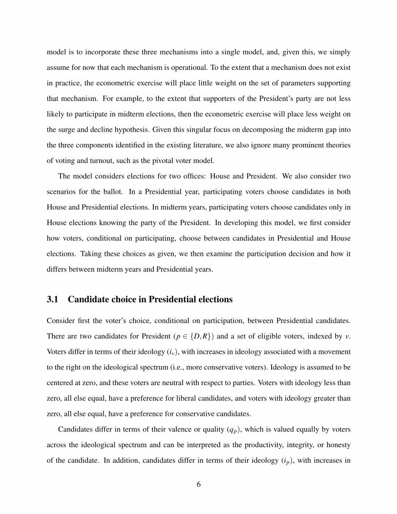
to follow. Also, let ωH denote the importance of ideology for voters in House elections, and let κH

represent polarization between House candidates.

In a House election held during a Presidential year, there is no consideration of punishing the

party of the sitting President in the model. We thus have the following for elections to the House

during Presidential years:

Uvh = −ωH

2(iv− ip)

2

∆Hv = ω

Hκ

H iv

Again, voters, conditional on participating, support the Republican House candidate (RH = 1) if

and only if ∆Hv > 0, and this is more likely when voters are right-leaning.

During midterm years, we allow for the possibility of a penalty against the party of the sit-

ting President. Let I ∈ {0,1} indicate whether the incumbent President is a Republican during a

midterm year, and let ρ , which is hypothesized to be negative, denote a penalty in midterm years

imposed by voters on the President’s party. Then, we have that:

∆Hv = ω

Hκ

H iv +ρ(2I−1)

As shown, when the incumbent President is a Republican, the willingness to support Republican

House candidates falls. Likewise, when the President is a Democrat, the willingness of voters to

support Republican House candidates increases.

3.3 Participation decision

Recall that the idea behind the revised theory of surge and decline is that the voters from the advan-

taged party in Presidential elections are energized to vote and that voters from the disadvantaged

party are cross-pressured and may choose to abstain. One natural way to formalize this notion is

8

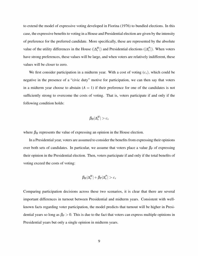
to extend the model of expressive voting developed in Fiorina (1976) to bundled elections. In this

case, the expressive benefits to voting in a House and Presidential election are given by the intensity

of preference for the preferred candidate. More specifically, these are represented by the absolute

value of the utility differences in the House (|∆Hv |) and Presidential elections (|∆P

v |). When voters

have strong preferences, these values will be large, and when voters are relatively indifferent, these

values will be closer to zero.

We first consider participation in a midterm year. With a cost of voting (cv), which could be

negative in the presence of a “civic duty” motive for participation, we can then say that voters

in a midterm year choose to abstain (A = 1) if their preference for one of the candidates is not

sufficiently strong to overcome the costs of voting. That is, voters participate if and only if the

following condition holds:

βH |∆Hv |> cv

where βH represents the value of expressing an opinion in the House election.

In a Presidential year, voters are assumed to consider the benefits from expressing their opinions

over both sets of candidates. In particular, we assume that voters place a value βP of expressing

their opinion in the Presidential election. Then, voters participate if and only if the total benefits of

voting exceed the costs of voting:

βH |∆Hv |+βP|∆P

v |> cv

Comparing participation decisions across these two scenarios, it is clear that there are several

important differences in turnout between Presidential and midterm years. Consistent with well-

known facts regarding voter participation, the model predicts that turnout will be higher in Presi-

dential years so long as βP > 0. This is due to the fact that voters can express multiple opinions in

Presidential years but only a single opinion in midterm years.

9

3.4 Midterm gaps and Mechanisms

Figures 1-4 summarize the three mechanisms through which this simple model generates midterm

gaps, defined as a loss in support for the President’s party during midterm years. In each graph,

the left side depicts a Presidential year, and the right side depicts a midterm year. In this graphical

summary, we assume that voter ideology is normally distributed in the baseline case to be described

below. We also assume that voters have identical and positive costs of voting (cv = c > 0, for all

v). Neither of these assumptions is critical for the results, and both will be relaxed in the empirical

analysis to follow.

Figure 1 illustrates the baseline case of no midterm gap. We assume here that (A) there is

no Presidential penalty in midterm years (ρ = 0), (B) there is no difference in quality between

the two Presidential candidates (∆qP = 0), and (C) the distribution of voter ideology is stable

across Presidential and midterm years. Then, the indifferent voter in all elections has ideology

zero, and conditional on participating, voters with ideology above zero support the Republican

and voters with ideology below zero support the Democrat. In terms of the turnout decision,

voting costs, which, as noted above, are assumed to be uniform and positive for the purposes

of this graph, are represented by the dotted line. Voters receive an expressive benefit (b) from

voting in each election, and this is given by the solid line, which is V-shaped since the indifferent

voter receives no expressive benefits from voting and benefits increase as voters become more

ideologically extreme. In Presidential years, voters receive two such expressive benefits, and this

total benefit is given by the dashed line. Voters then choose to participate in Presidential years

when these combined expressive benefits exceed the costs of voting. As shown, this leads to

higher participation in Presidential years. In terms of electoral outcomes, the red area then depicts

those who participate and support the Republican, and the blue area depicts those who participate

and support the Democrat. As shown, Republican candidates receive 50 percent of the vote in all

three elections, and there is no midterm gap since the President’s party does not lose support in

midterm years.

10

0voter ideology

Presidential voting

0voter ideology

cost ben tot_ben

House voting in Presidential year

0voter ideology

cost ben

House voting in midterm year

Figure 1: Baseline scenario with no midterm gap

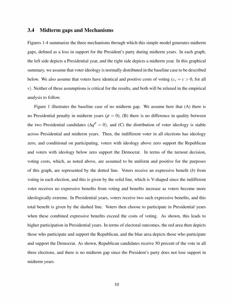
Figure 2 illustrates the case in which a midterm gap is due to a Presidential penalty in midterm

years (ρ < 0) but where the other two mechanisms are not in play. That is, we continue to as-

sume that there is no quality difference in the candidates for President and that the distribution of

voter ideology is stable across Presidential and midterm years. We generate a Presidential penalty

in midterm years by simply assuming that a Republican won the Presidential election via some

tiebreaker, such as the flip of the coin. Voters then respond to a Republican President by punishing

the party in the midterm year. In this case, the ideology of the indifferent voter in the midterm year

shifts to the right, expressive benefits of voting shift to the right, turnout increases on the left and

falls on the right, and the Republican vote share falls.9 To summarize, Figure 2 illustrates that a

simple preference for voting against the President’s party in midterm years generates a midterm

9While this graph depicts the Presidential penalty in midterm years arising from changes in turnout, it could also bedue to participants who shift their support to the Democrats in midterm years. To see this, consider the extreme case inwhich voting costs are zero for all voters and turnout is complete in both Presidential and midterm years. In this case,the Republican vote share will still fall due to moderate Republican voters shifting their support to the Democrats inthe midterm year.

11

gap.

0voter ideology

Presidential voting

0voter ideology

cost ben tot_ben

House voting in Presidential year

0voter ideology

cost ben

House voting in midterm year

Figure 2: Midterm Penalty with a Republican President

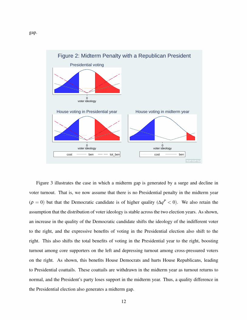
Figure 3 illustrates the case in which a midterm gap is generated by a surge and decline in

voter turnout. That is, we now assume that there is no Presidential penalty in the midterm year

(ρ = 0) but that the Democratic candidate is of higher quality (∆qP < 0). We also retain the

assumption that the distribution of voter ideology is stable across the two election years. As shown,

an increase in the quality of the Democratic candidate shifts the ideology of the indifferent voter

to the right, and the expressive benefits of voting in the Presidential election also shift to the

right. This also shifts the total benefits of voting in the Presidential year to the right, boosting

turnout among core supporters on the left and depressing turnout among cross-pressured voters

on the right. As shown, this benefits House Democrats and hurts House Republicans, leading

to Presidential coattails. These coattails are withdrawn in the midterm year as turnout returns to

normal, and the President’s party loses support in the midterm year. Thus, a quality difference in

the Presidential election also generates a midterm gap.

12

0voter ideology

Presidential voting

0voter ideology

cost ben tot_ben

House voting in Presidential year

0voter ideology

cost ben

House voting in midterm year

Figure 3: Surge and Decline

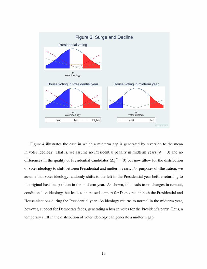
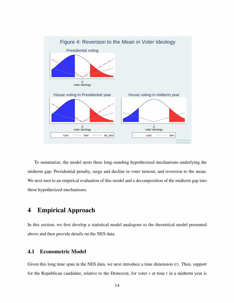
Figure 4 illustrates the case in which a midterm gap is generated by reversion to the mean

in voter ideology. That is, we assume no Presidential penalty in midterm years (ρ = 0) and no

differences in the quality of Presidential candidates (∆qP = 0) but now allow for the distribution

of voter ideology to shift between Presidential and midterm years. For purposes of illustration, we

assume that voter ideology randomly shifts to the left in the Presidential year before returning to

its original baseline position in the midterm year. As shown, this leads to no changes in turnout,

conditional on ideology, but leads to increased support for Democrats in both the Presidential and

House elections during the Presidential year. As ideology returns to normal in the midterm year,

however, support for Democrats fades, generating a loss in votes for the President’s party. Thus, a

temporary shift in the distribution of voter ideology can generate a midterm gap.

13

0voter ideology

Presidential voting

0voter ideology

cost ben tot_ben

House voting in Presidential year

0voter ideology

cost ben

House voting in midterm year

Figure 4: Reversion to the Mean in Voter Ideology

To summarize, the model nests three long-standing hypothesized mechanisms underlying the

midterm gap: Presidential penalty, surge and decline in voter turnout, and reversion to the mean.

We next turn to an empirical evaluation of this model and a decomposition of the midterm gap into

these hypothesized mechanisms.

4 Empirical Approach

In this section, we first develop a statistical model analogous to the theoretical model presented

above and then provide details on the NES data.

4.1 Econometric Model

Given this long time span in the NES data, we next introduce a time dimension (t). Then, support

for the Republican candidate, relative to the Democrat, for voter v at time t in a midterm year is

14

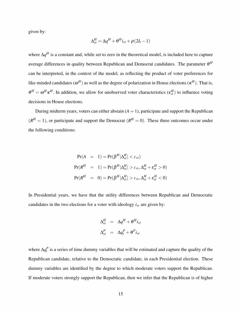
given by:

∆Hvt = ∆qH +θ

H ivt +ρ(2It−1)

where ∆qH is a constant and, while set to zero in the theoretical model, is included here to capture

average differences in quality between Republican and Democrat candidates. The parameter θ H

can be interpreted, in the context of the model, as reflecting the product of voter preferences for

like-minded candidates (ωH) as well as the degree of polarization in House elections (κH). That is,

θ H = ωHκH . In addition, we allow for unobserved voter characteristics (εHvt ) to influence voting

decisions in House elections.

During midterm years, voters can either abstain (A= 1), participate and support the Republican

(RH = 1), or participate and support the Democrat (RH = 0). These three outcomes occur under

the following conditions:

Pr(A = 1) = Pr(β H |∆Hvt |< cvt)

Pr(RH = 1) = Pr(β H |∆Hvt |> cvt ,∆

Hvt + ε

Hvt > 0)

Pr(RH = 0) = Pr(β H |∆Hvt |> cvt ,∆

Hvt + ε

Hvt < 0)

In Presidential years, we have that the utility differences between Republican and Democratic

candidates in the two elections for a voter with ideology ivt are given by:

∆Hvt = ∆qH +θ

H ivt

∆Pvt = ∆qP

t +θPivt

where ∆qPt is a series of time dummy variables that will be estimated and capture the quality of the

Republican candidate, relative to the Democratic candidate, in each Presidential election. These

dummy variables are identified by the degree to which moderate voters support the Republican.

If moderate voters strongly support the Republican, then we infer that the Republican is of higher

15

quality (∆qPt > 0). If moderate voters support the Democrat, by contrast, then we infer that the

Republican is of lower quality (∆qPt < 0).

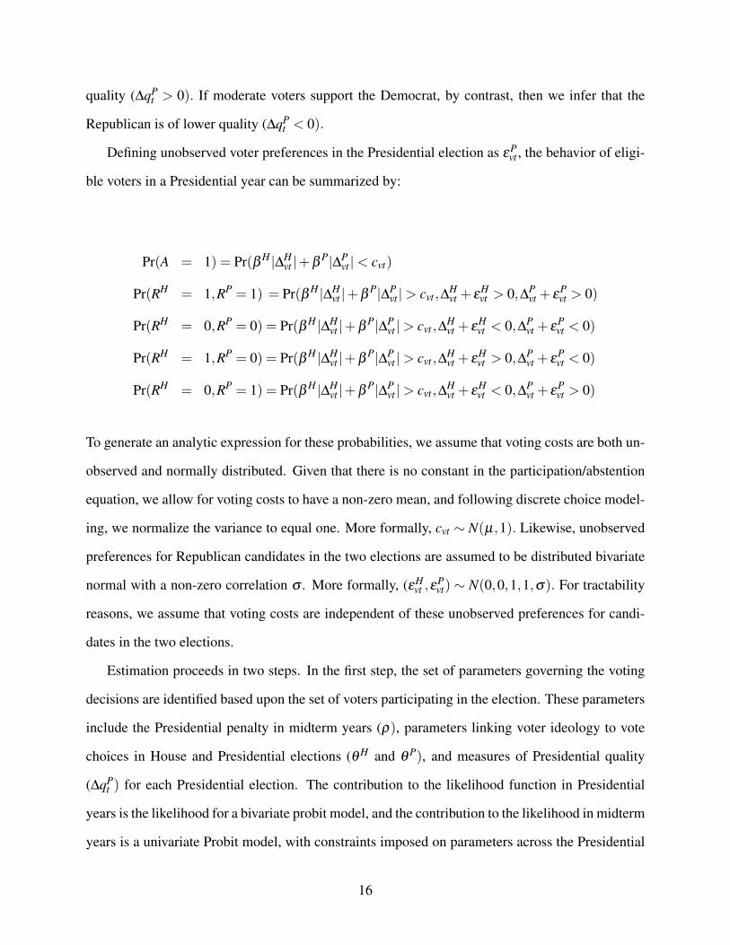
Defining unobserved voter preferences in the Presidential election as εPvt , the behavior of eligi-

ble voters in a Presidential year can be summarized by:

Pr(A = 1) = Pr(β H |∆Hvt |+β

P|∆Pvt |< cvt)

Pr(RH = 1,RP = 1) = Pr(β H |∆Hvt |+β

P|∆Pvt |> cvt ,∆

Hvt + ε

Hvt > 0,∆P

vt + εPvt > 0)

Pr(RH = 0,RP = 0) = Pr(β H |∆Hvt |+β

P|∆Pvt |> cvt ,∆

Hvt + ε

Hvt < 0,∆P

vt + εPvt < 0)

Pr(RH = 1,RP = 0) = Pr(β H |∆Hvt |+β

P|∆Pvt |> cvt ,∆

Hvt + ε

Hvt > 0,∆P

vt + εPvt < 0)

Pr(RH = 0,RP = 1) = Pr(β H |∆Hvt |+β

P|∆Pvt |> cvt ,∆

Hvt + ε

Hvt < 0,∆P

vt + εPvt > 0)

To generate an analytic expression for these probabilities, we assume that voting costs are both un-

observed and normally distributed. Given that there is no constant in the participation/abstention

equation, we allow for voting costs to have a non-zero mean, and following discrete choice model-

ing, we normalize the variance to equal one. More formally, cvt ∼ N(µ,1). Likewise, unobserved

preferences for Republican candidates in the two elections are assumed to be distributed bivariate

normal with a non-zero correlation σ . More formally, (εHvt ,ε

Pvt) ∼ N(0,0,1,1,σ). For tractability

reasons, we assume that voting costs are independent of these unobserved preferences for candi-

dates in the two elections.

Estimation proceeds in two steps. In the first step, the set of parameters governing the voting

decisions are identified based upon the set of voters participating in the election. These parameters

include the Presidential penalty in midterm years (ρ), parameters linking voter ideology to vote

choices in House and Presidential elections (θ H and θ P), and measures of Presidential quality

(∆qPt ) for each Presidential election. The contribution to the likelihood function in Presidential

years is the likelihood for a bivariate probit model, and the contribution to the likelihood in midterm

years is a univariate Probit model, with constraints imposed on parameters across the Presidential

16

and midterm years.

Given these estimated parameters from the first step, the expressive benefits of voting in House

(|∆Hvt |) and Presidential (|∆P

vt |) elections can be calculated, where the latter is simply set to zero

during midterm years, for both participants and non-participants. Then, these calculated expressive

benefits are included as generated regressors in a second stage univariate Probit equation examining

whether or not eligible voters choose to participate. This second stage employs information from

the entire sample and identifies the parameters linking expressive benefits to participation decisions

(β H and β P). Finally, bootstrap standard errors, using 1,000 replications, are calculated in order to

account for the uncertainty associated with using generated regressors in the second stage.

Given this setup, identification of the three key mechanisms underlying the midterm gap can

be summarized as follows. The Presidential penalty is identified by examining the degree to which

respondents, holding ideology fixed and conditional on participation, report voting against the

President’s party in midterm years. The surge and decline in voter turnout is identified by the

degree to which the participation margin is influenced by the intensity of preferences over the

Presidential candidates. Finally, mean reversion in ideology is identified by the degree to which

ideology shifts from year to year in aggregate and also by the degree to which ideology is linked

to choice of candidates.

4.2 Data

Our data comes from the American National Election Survey, which has been conducted in every

year with federal elections since 1948 except for the midterm years of 1950, 1954, 2006, and 2010.

Given that our key measure of voter ideology was not collected in 1948, we begin our sample in

1952 and thus have information from 15 Presidential years and from 12 midterm years, seven held

with a sitting Republican President and five with a sitting Democratic President.

Implementation of this empirical approach requires information on voter turnout decisions,

choice of House candidate, choice of Presidential candidate, and voter ideology. Measures of

turnout and voting decisions are based upon standard questions included in all years of the ANES.

17

The more complex issue involves the measurement of voter ideology. In order to capture the

possibility of mean reversion in explaining the midterm gap, we require a measure that is both

comparable across years and time-varying.10 Given this, we use two measures of self-reported

ideology that are comparable across years and time-varying.

The first measure is included in all survey years since 1952 and is based upon self-reported

party affiliation. There are seven possible responses to this question: 1) Strong Democrat, 2) Weak

Democrat, 3) Independent - leaning Democrat, 4) Independent - Independent, 5) Independent -

leaning Republican, 6) Weak Republican, and 7) Strong Republican. For consistency with the

theoretical model, we convert this measure to a [−1,1] interval, with Strong Democrat scoring

−1, Weak Democrat scoring−0.67, Independent - leaning Democrat scoring−0.33, Independent-

Independent scoring 0, Independent - leaning Republican scoring 0.33, Weak Republican scoring

0.67 and, finally, Strong Republican scoring 1.

One limitation of this measure of ideology is that it captures attachment to parties, which may

not respond to short-term forces, and this stability of party identification may lead us to understate

the contribution of the reversion to the mean mechanism. As an alternative measure, which per-

haps more closely captures voter ideology, we use voter thermometer scores of conservatives and

liberals. In particular, respondents were asked to rate conservatives on a 0 to 100 scale and were

asked to rate liberals on a 0 to 100 scale. We take the difference between these scores (conservative

score minus liberal score), which covers the interval [−100,100], and then convert this measure to

the [−1,1] interval by dividing by 100. Those providing the same thermometer score to Democrats

and Republicans receive a score of 0, those that provide a higher score to liberals have a negative

score, and those providing a higher score to conservatives have a positive score. One drawback of

this measure is that it is not available until 1964 and was also not included in the 1978 midterm

year survey. Given this more limited availability over time, we view this measure as providing a

robustness check on our baseline measure of party affiliation.

10One option would be to parameterize ideology as a function of demographics, exploiting the fact, for example,that women tend to be more supportive of Democrats than men. The problem here is that this measure will not betime-varying, absent dramatic changes in demographics, and thus will not capture high frequency change in ideologyunderlying the reversion to the mean hypothesis.

18

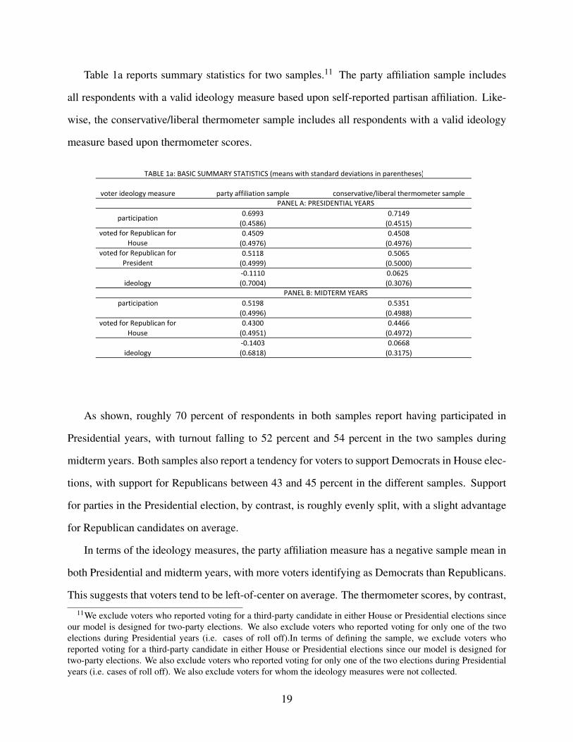
Table 1a reports summary statistics for two samples.11 The party affiliation sample includes

all respondents with a valid ideology measure based upon self-reported partisan affiliation. Like-

wise, the conservative/liberal thermometer sample includes all respondents with a valid ideology

measure based upon thermometer scores.

voter ideology measure party affiliation sample conservative/liberal thermometer sample

0.6993 0.7149(0.4586) (0.4515)0.4509 0.4508(0.4976) (0.4976)0.5118 0.5065(0.4999) (0.5000)‐0.1110 0.0625(0.7004) (0.3076)

participation 0.5198 0.5351(0.4996) (0.4988)0.4300 0.4466(0.4951) (0.4972)‐0.1403 0.0668(0.6818) (0.3175)

TABLE 1a: BASIC SUMMARY STATISTICS (means with standard deviations in parentheses)

ideology

voted for Republican for House

voted for Republican for President

voted for Republican for House

participation

ideology

PANEL A: PRESIDENTIAL YEARS

PANEL B: MIDTERM YEARS

As shown, roughly 70 percent of respondents in both samples report having participated in

Presidential years, with turnout falling to 52 percent and 54 percent in the two samples during

midterm years. Both samples also report a tendency for voters to support Democrats in House elec-

tions, with support for Republicans between 43 and 45 percent in the different samples. Support

for parties in the Presidential election, by contrast, is roughly evenly split, with a slight advantage

for Republican candidates on average.

In terms of the ideology measures, the party affiliation measure has a negative sample mean in

both Presidential and midterm years, with more voters identifying as Democrats than Republicans.

This suggests that voters tend to be left-of-center on average. The thermometer scores, by contrast,11We exclude voters who reported voting for a third-party candidate in either House or Presidential elections since

our model is designed for two-party elections. We also exclude voters who reported voting for only one of the twoelections during Presidential years (i.e. cases of roll off).In terms of defining the sample, we exclude voters whoreported voting for a third-party candidate in either House or Presidential elections since our model is designed fortwo-party elections. We also exclude voters who reported voting for only one of the two elections during Presidentialyears (i.e. cases of roll off). We also exclude voters for whom the ideology measures were not collected.

19

have positive sample means, with voters giving higher scores on average to conservatives than to

liberals. This suggests that voters tend to be right-of-center on average.

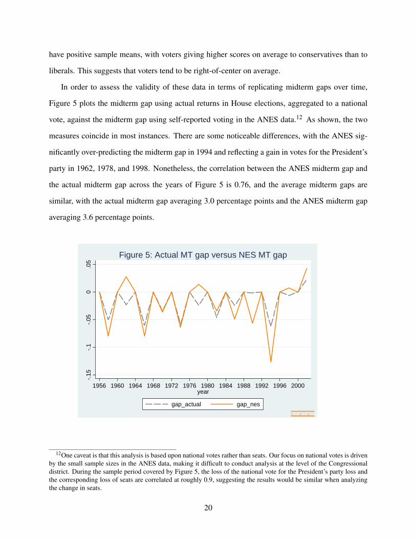
In order to assess the validity of these data in terms of replicating midterm gaps over time,

Figure 5 plots the midterm gap using actual returns in House elections, aggregated to a national

vote, against the midterm gap using self-reported voting in the ANES data.12 As shown, the two

measures coincide in most instances. There are some noticeable differences, with the ANES sig-

nificantly over-predicting the midterm gap in 1994 and reflecting a gain in votes for the President’s

party in 1962, 1978, and 1998. Nonetheless, the correlation between the ANES midterm gap and

the actual midterm gap across the years of Figure 5 is 0.76, and the average midterm gaps are

similar, with the actual midterm gap averaging 3.0 percentage points and the ANES midterm gap

averaging 3.6 percentage points.

-.15

-.1-.0

50

.05

1956 1960 1964 1968 1972 1976 1980 1984 1988 1992 1996 2000year

gap_actual gap_nes

Figure 5: Actual MT gap versus NES MT gap

12One caveat is that this analysis is based upon national votes rather than seats. Our focus on national votes is drivenby the small sample sizes in the ANES data, making it difficult to conduct analysis at the level of the Congressionaldistrict. During the sample period covered by Figure 5, the loss of the national vote for the President’s party loss andthe corresponding loss of seats are correlated at roughly 0.9, suggesting the results would be similar when analyzingthe change in seats.

20

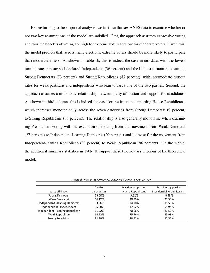
Before turning to the empirical analysis, we first use the raw ANES data to examine whether or

not two key assumptions of the model are satisfied. First, the approach assumes expressive voting

and thus the benefits of voting are high for extreme voters and low for moderate voters. Given this,

the model predicts that, across many elections, extreme voters should be more likely to participate

than moderate voters. As shown in Table 1b, this is indeed the case in our data, with the lowest

turnout rates among self-declared Independents (36 percent) and the highest turnout rates among

Strong Democrats (73 percent) and Strong Republicans (82 percent), with intermediate turnout

rates for weak partisans and independents who lean towards one of the two parties. Second, the

approach assumes a monotonic relationship between party affiliation and support for candidates.

As shown in third column, this is indeed the case for the fraction supporting House Republicans,

which increases monotonically across the seven categories from Strong Democrats (9 percent)

to Strong Republicans (88 percent). The relationship is also generally monotonic when examin-

ing Presidential voting with the exception of moving from the movement from Weak Democrat

(27 percent) to Independent-Leaning Democrat (20 percent) and likewise for the movement from

Independent-leaning Republican (88 percent) to Weak Republican (86 percent). On the whole,

the additional summary statistics in Table 1b support these two key assumptions of the theoretical

model.

fraction fraction supporting fraction supportingparty affiliation participating House Republicans Presidential RepublicansStrong Democrat 73.00% 9.12% 8.48%Weak Democrat 56.12% 20.99% 27.33%

Independent ‐ leaning Democrat 53.96% 24.20% 19.53%Independent ‐ Independent 35.88% 47.02% 59.94%

Independent ‐ leaning Republican 61.52% 70.66% 87.59%Weak Republican 64.52% 75.56% 85.98%Strong Republican 82.39% 88.42% 97.56%

TABLE 1b: VOTER BEHAVIOR ACCORDING TO PARTY AFFILIATION

21

5 Results

5.1 Descriptive Evidence

Before turning to the econometric evidence, we first provide a comparison (Presidential versus

midterm years) of the three key mechanisms in the model. Motivated by the key prediction that

voters with ideology favoring the President’s party should be less likely to participate in midterm

years, when compared to previous Presidential election, we first examine how turnout changes for

voters of differing ideology between Presidential and midterm years. To make ideology compara-

ble across Republican and Democratic Presidents, we define President’s party ideology equal to ivt

when the President is a Republican and equal to −ivt when the President is Democrat.13

As shown in Figure 6 and consistent with Table 1b, turnout rates exhibit the V-shaped pattern

predicted by the model in both Presidential and midterm years, and turnout is higher for all groups

in Presidential years when compared to midterm years. Figure 6 also provides some evidence

favoring the surge and decline hypothesis. In particular, for the three groups with President’s party

ideology greater than zero, the drop off in turnout when moving from Presidential to midterm years

averages 17.5 percentage points, while the drop off averages 15.7 percentage points for the groups

with President’s ideology less than zero.

13For example, President’s party ideology equals +1 when the President is a Republican and the voter is classifiedas strong Republican or when the President is a Democrat and the voter is classified as strong Democrat.

22

.3.4

.5.6

.7.8

fract

ion

vote

d

-1 -.5 0 .5 1President's party ideology

Presidential year Midterm year

Figure 6: Turnout in Presidential and Midterm Years

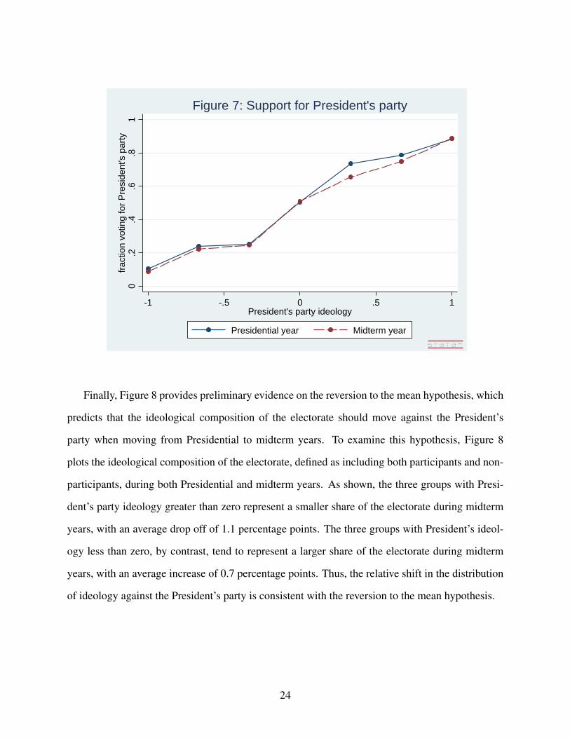
Figure 7 provides descriptive evidence on the Presidential penalty hypothesis by focusing on

electoral support for the President’s party, conditional on participation, during Presidential and

midterm years and separately by President’s party ideology. As shown, four of the seven ideo-

logical groups do exhibit noticeable drops in support for the President’s party when moving from

Presidential to midterm years, and none of the seven groups exhibit an increase in support for the

President’s party. Averaged across the seven groups, the loss in support for the President’s party is

equal to 2.2 percentage points.

23

0.2

.4.6

.81

fract

ion

votin

g fo

r Pre

side

nt's

par

ty

-1 -.5 0 .5 1President's party ideology

Presidential year Midterm year

Figure 7: Support for President's party

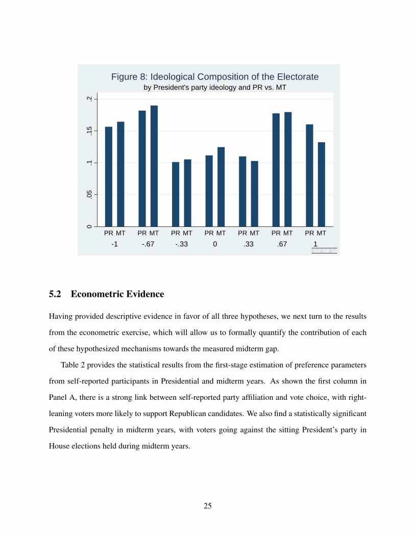
Finally, Figure 8 provides preliminary evidence on the reversion to the mean hypothesis, which

predicts that the ideological composition of the electorate should move against the President’s

party when moving from Presidential to midterm years. To examine this hypothesis, Figure 8

plots the ideological composition of the electorate, defined as including both participants and non-

participants, during both Presidential and midterm years. As shown, the three groups with Presi-

dent’s party ideology greater than zero represent a smaller share of the electorate during midterm

years, with an average drop off of 1.1 percentage points. The three groups with President’s ideol-

ogy less than zero, by contrast, tend to represent a larger share of the electorate during midterm

years, with an average increase of 0.7 percentage points. Thus, the relative shift in the distribution

of ideology against the President’s party is consistent with the reversion to the mean hypothesis.

24

0.0

5.1

.15

.2

-1 -.67 -.33 0 .33 .67 1PR MT PR MT PR MT PR MT PR MT PR MT PR MT

by President's party ideology and PR vs. MTFigure 8: Ideological Composition of the Electorate

5.2 Econometric Evidence

Having provided descriptive evidence in favor of all three hypotheses, we next turn to the results

from the econometric exercise, which will allow us to formally quantify the contribution of each

of these hypothesized mechanisms towards the measured midterm gap.

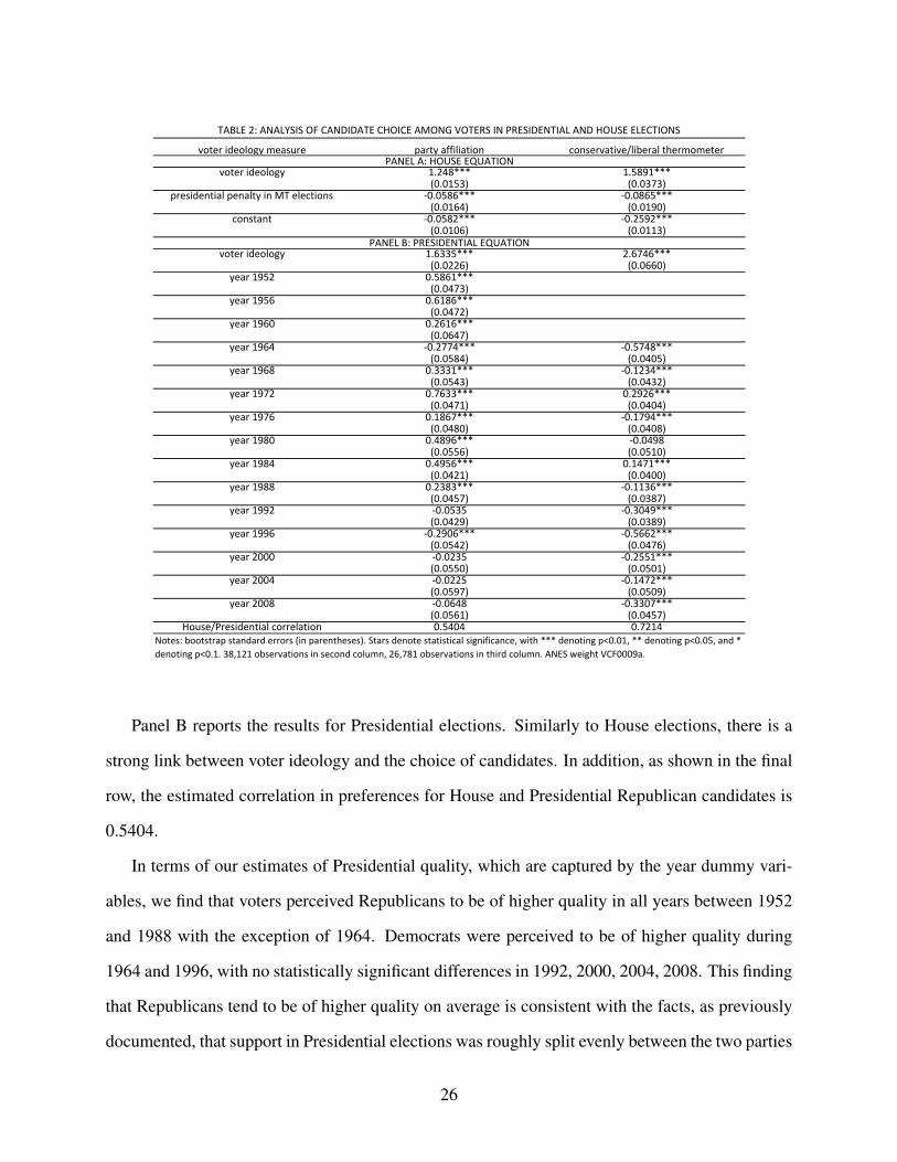
Table 2 provides the statistical results from the first-stage estimation of preference parameters

from self-reported participants in Presidential and midterm years. As shown the first column in

Panel A, there is a strong link between self-reported party affiliation and vote choice, with right-

leaning voters more likely to support Republican candidates. We also find a statistically significant

Presidential penalty in midterm years, with voters going against the sitting President’s party in

House elections held during midterm years.

25

voter ideology measure party affiliation conservative/liberal thermometer

voter ideology 1.248*** 1.5891***(0.0153) (0.0373)

presidential penalty in MT elections ‐0.0586*** ‐0.0865***(0.0164) (0.0190)

constant ‐0.0582*** ‐0.2592***(0.0106) (0.0113)

voter ideology 1.6335*** 2.6746***(0.0226) (0.0660)

year 1952 0.5861***(0.0473)

year 1956 0.6186***(0.0472)

year 1960 0.2616***(0.0647)

year 1964 ‐0.2774*** ‐0.5748***(0.0584) (0.0405)

year 1968 0.3331*** ‐0.1234***(0.0543) (0.0432)

year 1972 0.7633*** 0.2926***(0.0471) (0.0404)

year 1976 0.1867*** ‐0.1794***(0.0480) (0.0408)

year 1980 0.4896*** ‐0.0498(0.0556) (0.0510)

year 1984 0.4956*** 0.1471***(0.0421) (0.0400)

year 1988 0.2383*** ‐0.1136***(0.0457) (0.0387)

year 1992 ‐0.0535 ‐0.3049***(0.0429) (0.0389)

year 1996 ‐0.2906*** ‐0.5662***(0.0542) (0.0476)

year 2000 ‐0.0235 ‐0.2551***(0.0550) (0.0501)

year 2004 ‐0.0225 ‐0.1472***(0.0597) (0.0509)

year 2008 ‐0.0648 ‐0.3307***(0.0561) (0.0457)

House/Presidential correlation 0.5404 0.7214

TABLE 2: ANALYSIS OF CANDIDATE CHOICE AMONG VOTERS IN PRESIDENTIAL AND HOUSE ELECTIONS

Notes: bootstrap standard errors (in parentheses). Stars denote statistical significance, with *** denoting p<0.01, ** denoting p<0.05, and * denoting p<0.1. 38,121 observations in second column, 26,781 observations in third column. ANES weight VCF0009a.

PANEL A: HOUSE EQUATION

PANEL B: PRESIDENTIAL EQUATION

Panel B reports the results for Presidential elections. Similarly to House elections, there is a

strong link between voter ideology and the choice of candidates. In addition, as shown in the final

row, the estimated correlation in preferences for House and Presidential Republican candidates is

0.5404.

In terms of our estimates of Presidential quality, which are captured by the year dummy vari-

ables, we find that voters perceived Republicans to be of higher quality in all years between 1952

and 1988 with the exception of 1964. Democrats were perceived to be of higher quality during

1964 and 1996, with no statistically significant differences in 1992, 2000, 2004, 2008. This finding

that Republicans tend to be of higher quality on average is consistent with the facts, as previously

documented, that support in Presidential elections was roughly split evenly between the two parties

26

but that voters were more likely to identify as Democrats. The coexistence of these two facts re-

quires that Democratic-identifying voters are more likely to support Republican candidates, when

compared to the rate of crossing party lines in Presidential elections for Republican-identifying

voters.

Note that the variation in quality across Presidential years is identified via a revealed preference

approach. That is, candidates receiving more support among voters, holding fixed participation and

voter ideology, are inferred to be of higher quality. One important alternative interpretation of these

quality measures involves candidate ideology. In particular, it is possible that candidates receiving

more support among voters are more moderate, rather than of higher quality. For example, our

finding that Reagan was of much higher quality than Mondale in 1980 may instead reflect the

fact that Mondale was viewed by voters as being too liberal. To address this concern, we have

incorporated measures of voter perceptions of the ideology of Presidential candidates, measured

in the ANES starting in 1972 on a seven point scale, ranging from extremely liberal to extremely

conservative. After scaling this variable to be centered at zero and ranging from−1 to +1, we next

calculate the ideological preference for the Republican (ideology iR) over the Democrat (ideology

iD) for voter v as follows:

−(iv− iR)2 +(iv− iD)2

Consistent with the theoretical model, this measure captures the quadratic distance between voter

ideology and the ideology of the Republican candidate, relative to the Democratic candidate. Under

the baseline assumption that iR =−iD = κP/2, this ideological preference collapses to 2κPiv. More

generally, however, voters have a preference for moderate candidates, and, in this more general

case, quality can then be inferred conditional on measures of voter perceptions of the ideology of

the two candidates. Having estimated this extended model using the years starting in 1972 and

having also estimated the baseline model using only years starting in 1972, the correlation in the

candidate quality measures is over 0.97. This high correlation between our baseline measures of

27

quality and these measures that account for candidate ideology suggests that our quality measures

are not capturing differences in candidate ideology.14

Returning to our baseline estimates in Table 2, we then compute the expressive benefits to

voting in both Presidential and midterm years for both participants and non-participants. In Presi-

dential years, we separately compute the benefits to voting in the House elections and the benefits

to voting in Presidential elections. In the midterm year, by contrast, we set the benefits to voting in

the Presidential election to zero.

Using these constructed measures of the expressive benefits of voting, we then examine how

they impact turnout decisions. As shown in the first column of Table 3, the positive coefficients

for both House and Presidential elections make clear that the expressive benefits of voting in both

types of elections increase voter turnout, with the benefits from expressing support in the House

election playing a somewhat stronger role.

0.5136*** 0.6063***(0.0218) (0.0258)0.3972*** 0.2195***(0.0138) (0.0229)

0.3124*** 0.3918***(0.0178) (0.0208)0.2115*** 0.1018***(0.0107) (0.0111)

0.265*** 0.3508***(0.0266) (0.0196)

‐0.3080*** ‐0.4268*** ‐0.088*** ‐0.2573***(0.0165) (0.0215) (0.0125) (0.0170)

TABLE 3: TURNOUT DECISION WITH PARTY AFFILIATION MEASURE OF IDEOLOGY

Notes: bootstrap standard errors (in parentheses). Stars denote statistical significance, with *** denoting p<0.01, ** denoting p<0.05, and * denoting p<0.1. 38,121 observations. Preference difference measures for President set to zero during midterm election years. Preference difference measures inferred from column 2 of Table 2. ANES weight VCF0009a.

absolute preference difference House

absolute preference difference Presidentsquared preference difference Housesquared preference difference President

presidential year

constant

Since the expressive benefits from voting in the Presidential election is by construction zero

during midterm years, one alternative explanation for the positive coefficient on the expressive

benefits of voting in Presidential elections is that turnout is higher in Presidential years for reasons

14These two sets of estimates are available upon request from the author.

28

that are not captured in our model. While there is no reason to believe that the economic costs

of voting should be different between Presidential and midterm years, one could imagine that

civic duty considerations are stronger in Presidential years. That is, there may be non-expressive

benefits of voting in Presidential years, boosting turnout. We recognize this alternative explanation

and attempt to address this in column (2) of Table 3 by including an indicator for Presidential

years. In this case, the coefficient on the expressive benefits of voting in the Presidential election

are identified by variation in the quality of Presidential candidates across different Presidential

elections. As shown, while this key coefficient does fall in magnitude, it remains positive and

statistically significant.

As a robustness check, we next run the second stage regressions using an alternative measure

of the expressive benefits of voting based upon the squared, rather than absolute, difference in pref-

erences over the candidates. That is, instead of calculating absolute differences in House elections,

|∆Hvt |, we calculate (∆H

vt)2, and we define analogous measures in Presidential elections. In this case,

expressive benefits are convex, rather than linear, in the difference in preferences over candidates.

As shown in column (3) of Table 3, the results are similar in sign to the baseline results in column

(1). Finally, as shown in column (4), these results are also robust to using this squared measure of

expressive benefits and the inclusion of an indicator for Presidential years.

Returning to Table 2, we next conduct the analysis using the conservative-liberal thermometer

measure of voter ideology. As shown in column (2), the coefficients on voter ideology remain

positive and statistically significant.15 As shown in the final row, the estimated correlation in

preferences for House and Presidential Republican candidates in this case is 0.7214. Finally, the

quality measures, with the exception of 1984, are strongly negative, suggesting that Democrats are

more appealing to swing voters, defined as those close to zero in this ideology measure. As noted

above, this is consistent with voters having more right-leaning ideology using this measure and

votes being roughly split between the two parties in Presidential elections.

Finally, Table 4 provides the turnout results using this alternative ideology measure. As shown,

15Note that the coefficients in column 2 are not directly comparable to those in column 1 since the variance of theunobserved components may differ across these specifications.

29

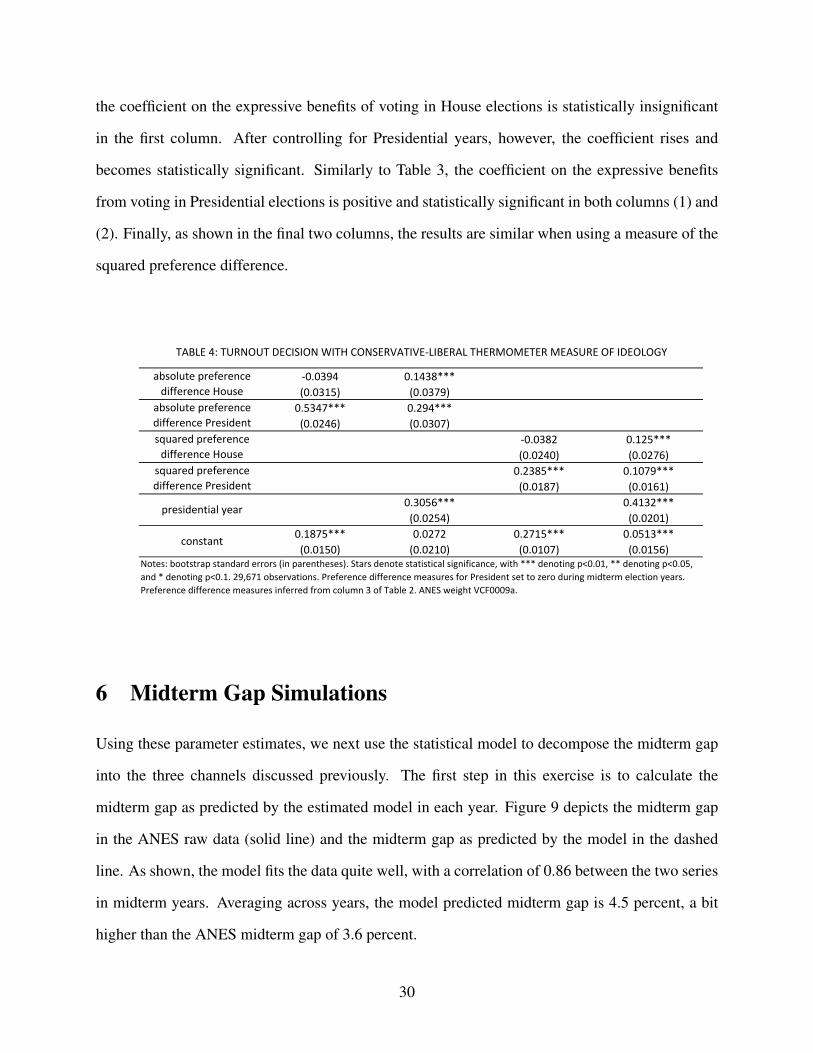
the coefficient on the expressive benefits of voting in House elections is statistically insignificant

in the first column. After controlling for Presidential years, however, the coefficient rises and

becomes statistically significant. Similarly to Table 3, the coefficient on the expressive benefits

from voting in Presidential elections is positive and statistically significant in both columns (1) and

(2). Finally, as shown in the final two columns, the results are similar when using a measure of the

squared preference difference.

‐0.0394 0.1438***(0.0315) (0.0379)0.5347*** 0.294***(0.0246) (0.0307)

‐0.0382 0.125***(0.0240) (0.0276)0.2385*** 0.1079***(0.0187) (0.0161)

0.3056*** 0.4132***(0.0254) (0.0201)

0.1875*** 0.0272 0.2715*** 0.0513***(0.0150) (0.0210) (0.0107) (0.0156)

constant

Notes: bootstrap standard errors (in parentheses). Stars denote statistical significance, with *** denoting p<0.01, ** denoting p<0.05, and * denoting p<0.1. 29,671 observations. Preference difference measures for President set to zero during midterm election years. Preference difference measures inferred from column 3 of Table 2. ANES weight VCF0009a.

TABLE 4: TURNOUT DECISION WITH CONSERVATIVE‐LIBERAL THERMOMETER MEASURE OF IDEOLOGY

absolute preference difference House

absolute preference difference Presidentsquared preference difference Housesquared preference difference President

presidential year

6 Midterm Gap Simulations

Using these parameter estimates, we next use the statistical model to decompose the midterm gap

into the three channels discussed previously. The first step in this exercise is to calculate the

midterm gap as predicted by the estimated model in each year. Figure 9 depicts the midterm gap

in the ANES raw data (solid line) and the midterm gap as predicted by the model in the dashed

line. As shown, the model fits the data quite well, with a correlation of 0.86 between the two series

in midterm years. Averaging across years, the model predicted midterm gap is 4.5 percent, a bit

higher than the ANES midterm gap of 3.6 percent.

30

-.15

-.1-.0

50

.05

1956 1960 1964 1968 1972 1976 1980 1984 1988 1992 1996 2000year

gap_model gap_nes

Figure 9: NES MT gap versus model predicted MT gap

We next decompose the model predicted midterm gap into its three components. We do so

by removing the mechanisms one at a time. Removing the Presidential penalty mechanism is

achieved quite simply by setting the penalty in midterm years to zero (ρ = 0). This requires that

voting probabilities in House elections, conditional on ideology and participation, are identical

in midterm and Presidential years and also are independent of the Presidential party in power in

midterm years.

Likewise, removing the surge and decline mechanism can be achieved by setting the coefficient

on the expressive benefits to voting in Presidential elections to zero (β P = 0). This requires that

turnout in Presidential and midterm years is identical and thus changes in the composition of the

electorate when moving from Presidential to midterm years cannot lead to a reduction in support

for the President’s party.

Finally, removing reversion to the mean in voter ideology is achieved by holding fixed the dis-

tribution of voter ideology when moving from a Presidential year to the subsequent midterm year.

31

Operationally, we do this by using only the sample of voters in Presidential years and then, hold-

ing only their ideology constant, predict both their choice over candidates and their participation

decision in the subsequent midterm year environment.

Figure 10 displays the results from these calculations. The black line represents the midterm

gap predicted by the model and it identical to that in Figure 9. The blue line represents the midterm

gap without the Presidential penalty mechanism. The red line represents the midterm gap without

surge and decline. Finally, the yellow line represents the midterm gap without mean reversion in

voter ideology.

-.1-.0

50

.05

1956 1960 1964 1968 1972 1976 1980 1984 1988 1992 1996 2000year

gap_model gap_no_referendumgap_no_surge gap_no_mean_reversion

Figure 10: MT gap decomposition

As shown, removing the Presidential penalty unambiguously benefits the President’s party,

with smaller losses in years with midterm losses and larger gains in years with midterm gains. The

surge and decline and mean reversion mechanisms, by contrast, appear to be moderating forces.

That is, removing these mechanisms tends to push midterm gaps towards zero in years with both

midterm losses and years with midterm gains.

32

To get a sense of the contribution of these factors on average, we next average these contribu-

tions across all midterm years. According to these calculations, the Presidential penalty mechanism

plays the largest role, with the midterm gap falling from 4.5 percent on average to 2.4 percent in the

absence of this mechanism. The fact that midterm gap falls significantly when removing the Pres-

idential penalty mechanism implies that this mechanism is important in explaining the midterm

gap. In particular, we can say that this mechanism explains 47 percent of the midterm gap when

averaged across years. In the absence of either of the other two mechanisms, by contrast, the

midterm gap falls to 3.3 percent. Thus, we can say that surge and decline and mean reversion in

voter ideology each explain 27 percent of the midterm gap.

We next repeat these decompositions based upon the analysis using the conservative/liberal

thermometer measure underlying the results in column (2) of Table 2 and Table 4. The Presidential

penalty hypothesis again plays the largest role here. Eliminating this mechanism leads the midterm

gap to fall from its predicted value of 4.2 percent to just 1.2 percent. Thus, the Presidential penalty

mechanism here explains a large fraction, 72 percent, of the midterm gap predicted by the model.

The surge and decline mechanism explains 17 percent, and mean reversion in voter ideology ex-

plains 11 percent. Thus, this analysis using an alternative measure voter ideology places a larger

emphasis on the Presidential penalty hypothesis.

7 Conclusion

In summary, this paper has provided an investigation of three long-standing explanations for the

midterm gap. These hypothesized explanations include the Presidential penalty in midterm years,

a surge and decline in voter turnout, and mean reversion in voter ideology. These mechanisms are

developed in the context of a model in which voters decide both whether or not to participate in

midterm and Presidential years and, conditional on participating, which candidates to support. The

parameters of this model are then estimated, and counterfactual simulations allow for the decom-

position of the midterm gap into the contributions from these three hypothesized mechanisms.

33

It is important to note several limitations of this analysis. First, this analysis does not address

some explanations for the midterm gap, such as the informational spillovers hypothesis put forward

by Halberstam and Montagnes (2014). Second, the analysis cannot distinguish between competing

explanations underlying the Presidential penalty in midterm years. These include voters using

midterm years as a referendum on the President’s performance and voter preferences for divided

government. Third, the analysis does not incorporate the possibility of selective abstention or roll-

off, under which voters may choose to participate in the Presidential election but not the House

election during Presidential years.16 This may tend to weaken the surge and decline mechanism,

which highlights the impact of changing incentives for turnout in the Presidential election on House

elections during Presidential years. That is, some voters who turn out in Presidential years but not

House years will selectively abstain from the House election during Presidential years. Thus, these

voters will not cast voters for House elections in either year and thus cannot play a role in the

midterm gap.

Although the quantitative results vary across specifications, there are a few general lessons to

be taken away from the analysis. First, the estimated model matches well the observed midterm

gap over time and can fully explain the midterm gap when averaged across midterm years. Second,

each of the three mechanisms, as formalized in the theoretical model and estimated in the empirical

analysis, plays a substantive role in explaining the midterm gap. Finally, while this lesson is

more sensitive to the specification, the bulk of the evidence points towards the Presidential penalty

hypothesis playing a stronger role than surge and decline and a reversion to the mean in voter

ideology.

16On the issue of selective abstention, see Degan and Merlo (2011).

34

References

Alesina, Alberto, and Howard Rosenthal. 1989. “Partisan cycles in congressional elections and

the macroeconomy.” American Political Science Review 83(2): 373-398.

Alesina, Alberto, and Howard Rosenthal. 1996. “A theory of divided government”. Econometrica

64(6): 1311-1341.

Bafumi, Joseph, Robert S. Erikson, and Christopher Wlezien. 2010. “Balancing, generic polls

and midterm congressional elections.” Journal of Politics 72(3): 705-719.

Born, Richard. 1990. “Surge and decline, negative voting, and the midterm loss phenomenon: a

simultaneous choice analysis.” American Journal of Political Science 34(3): 615-645.

Campbell, Angus. 1960. “Surge and decline: a study of electoral change.” Public Opinion Quar-

terly 24(3): 397-418.

Campbell, James E. 1987. “The revised theory of surge and decline.” American Journal of Polit-

ical Science 31(4): 965-979.

Degan, Arianna and Merlo, Antonio. 2011. “A structural model of turnout and voting in multiple

election.” Journal of the European Economic Association 9(2): 209–245.

Erikson, Robert S. 2010. “Explaining midterm loss: the tandem effect of withdrawn coattails and

balancing.” Paper prepared for the 2010 Meeting of the American Political Science Associ-

ation, Washington, D.C.

Fair, Ray C. 2009. “Presidential and Congressional Vote-Share Equations.” American Journal of

Political Science 53(1): 55-72.

Fiorina, Morris P. 1976. “The voting decision: instrumental and expressive aspects.” Journal of

Politics 38(2): 390–413.

35

Folke, Olle, and James M. Snyder, Jr. 2012. “Gubernatorial midterm slumps”. American Journal

of Political Science 56(4): 931-948.

Halberstam, Yosh and Pablo Montagnes. 2014. “Presidential Coattails versus The Median Voter:

Senator Selection in U.S. Elections”, forthcoming, Journal of Public Economics.

Hinkley, Barbara, 1967. “Interpreting House Midterm Elections: Toward a Measurement of the

In-Party’s "Expected" Loss of Seats.” American Political Science Review 63(3): 694–700.

Levitt, Steven. 1994. “An Empirical Test of Competing Explanations for the Midterm Gap in the

US House.” Economics and Politics 6(1): 25–37.

McDonald, Michael D and Best, Robin. 2006. “Equilibria and restoring forces in models of vote

dynamic.” Political Analysis 14(4): 369–392.

Mebane, Jr., Walter. 2000. “Coordination, moderation, and institutional balancing in American

Presidential and House elections.” American Political Science Review 94(1): 37-57.

Mebane, Jr., Walter, and Jasjeet S. Sekhon. “Coordination and policy moderation at midterm.”

American Political Science Review 96(1): 141-157.

Oppenheimer, Bruce I and Stimson, James A and Waterman, Richard. 1986. “Interpreting US

Congressional Elections: The Exposure Thesis.” Legislative Studies Quarterly 11(2): 227–

247.

Scheve, Kenneth, and Michael Tomz. 1999. “Electoral surprise and the midterm loss in US

congressional elections.” British Journal of Political Science 29: 507-521.

Tufte, Edward R. 1975. “Determinants of the outcomes of midterm congressional elections.”

American Political Science Review 69(3): 812-826.

36