an econometric chronology of the financial crisis of...
TRANSCRIPT
An Econometric Chronology of the Financial Crisis of 2007-2008 *
Gary Gorton Yale School of Management and NBER
Andrew Metrick
Yale School of Management and NBER
Lei Xie AQR Capital
April 28, 2015
Abstract
What is a “financial crisis”? In this paper, we introduce a new definition: a financial crisis is defined as a common econometric breakpoint in the characteristics of different forms of bank-produced money. We use this methodology to document the crisis of 2007-2009. The empirical chronology is based on locating the dates of structural breaks in panel data sets, based on the technique of Bai (2010). In contrast to ex post narrative chronologies, the econometric chronology is based on contemporaneous market prices, and reveals precise steps in the crisis prior to the Lehman collapse.
*This paper was originally part of a paper entitled “The Flight from Maturity.” We thank Jushan Bai for constructing confidence intervals for his estimation procedure. We also thank a number of market participants (who wish to remain anonymous) for providing data. For comments and suggestions on the original paper, “The Flight from Maturity,” we thank Don Andrews, Simon Gilchrist, James Hamilton, Anna Kovner, Arvind Krishnamurthy, Pete Kyle, Andrew Morton, Tyler Muir and Harald Uhlig. Also, thanks to seminar participants at the 2013 AEA meetings, the 2012 Annual Bank of Canada Conference, the Wharton Conference on Liquidity and Financial Crises, the Board of Governors of the Federal Reserve System, the Princeton 2013 Julius-Rabinowitz Conference, the 2013 NBER Monetary Economics Meeting, the IMF and the Sixteenth Annual International Banking Conference at the Federal Reserve Bank of Chicago. Thanks to Arvind Krishnamurthy, Stefan Nagel, and Dmitry Orlov for sharing their repo maturity data from Krishnamurthy, Nagel and Orlov (2011).
1
1. Introduction
Crises are chaotic. Understanding the dynamics of the financial crisis of 2007-2009 requires determining
the timing of important events. Many crisis chronologies have been produced based on the
announcement dates of government or central bank actions and on the dates of various other public
events. These include chronologies have been assembled by newspapers and authors of books on the
crisis, as well as those put together by the Federal Reserve Bank of St. Louis, the Bank of England and the
European Central Bank, among others.1 We document the crisis chronology econometrically. Our dating
procedure is fundamentally different because it is based on locating the dates of structural breaks in
panel data sets of market prices (and repo haircuts), using the econometric methodology of Bai (2010).
Our chronology dates the first structural break in panels of spreads on subprime-related instruments, to
date the start of the crisis, and then the subsequent reactions of secured money market instruments
(repo), unsecured money market instruments (e.g., asset-backed commercial paper), credit derivative
(CDS) measures of the risk in financial firms, and finally, price-based measures of real economic activity.
We date the first breaks and also subsequent break dates. In this way we observe the evolution of the
crisis based on the actions of market participants.
A chronology of the crisis is also very important because it allows us to formalize the concept of a
financial crisis. What is a “crisis”? In this paper, we introduce a new definition: a financial crisis is
defined as a common breakpoint in the characteristics of different forms of bank-produced money (i.e.,
repo and asset-backed commercial paper (ABCP)). 2 The financial system becomes insolvent because in a
crisis short-term bank debt becomes suspect and banks are unable to satisfy demands for cash. Even the
determination of whether an event is a crisis, and when it starts and ends, is based on governments’
actions and other publicly observed events because these are readily observable. Boyd, De Nicolò and
1
Examples of chronologies assembled by newspapers include that of The Guardian (http://www.theguardian.com/business/2012/aug/07/credit-crunch-boom-bust-timeline) and that of USA Today (http://www.usatoday.com/story/money/business/2013/09/08/chronology-2008-financial-crisis-lehman/2779515/ ). CNBC has a chronology: http://www.cnbc.com/id/101019322#. The Federal Reserve Bank of St. Louis’ chronology can be found at http://timeline.stlouisfed.org/index.cfm?p=timeline and the Bank of England at http://www.bankofengland.co.uk/publications/Documents/fsr/2009/fsrannex0906.pdf; and the European Central Bank Chronology is here: https://www.ecb.europa.eu/ecb/html/crisis.en.html. Finally, many books on the crisis provide a chronology or have a narrative that follows events chronologically. Also, see Gorton (2010) and Wessel (2010). Sprague (1910) provides chronologies for panics during the U.S. National Banking Era. 2 Asset-backed commercial paper (ABCP) is commercial paper that is issued by conduits, which is a special purpose
vehicle (a legal entity) that buys asset-backed securities, financing this by issuing commercial paper. See Covitz, Liang, and Suarez (2009) and Acharya, Schnabl and Suarez (2011).

2
Loukoianova (2011) study the four leading classifications and dating of modern crisis events.3 They
show that for many crises the dating of the start and end dates differ quite significantly among different
researchers. There is also some disagreement on which events are, in fact, crises. Further, they show
that the start dates are late.4 The dating of the start and the end of a crisis is largely based on
contemporary accounts of the crisis, and there is ambiguity. We use daily price data to formalize the
crisis dating for the events of 2007-2009 and, in the process, understand crises.
Our approach allows for more precision on the start date, and also uncovers rich subsequent dynamics.
With respect to the concept of a crisis, an important finding is that the crisis starts with simultaneous
breakpoints in the repo and asset-backed commercial paper markets, in July 2007. At the same time,
the financial firms risk shows a break, as measured by their CDS spreads. Finally, and perhaps most
importantly, the spreads of non-mortgage asset-backed securities show a break. Another important
finding is that between the start of the crisis and the Lehman failure, there are a number of other
breakpoints in the money markets and in repo haircuts. The dynamics of the crisis leading up to Lehman
suggest that during a crisis, fragility is building up. . Similar results have been found by Ó Gráda and
White (2003) who study the panics of 1854 and 1857 based on the detailed records of the Emigrant
Savings Bank in New York City. They show that these events were not characterized by immediate mass
panic withdrawals from the bank. Depositors withdrew some, but not all of their money—akin to
haircuts rising but not going to 100 percent. Later they withdrew more. Also see Kelly and Ó Gráda
(2000) and Iyer and Puri (2012).
The crisis can be seen in Figure 1 which shows (annualized) spreads (relative to the overnight index swap
rate) on overnight loans.5 The figure shows spreads for federal funds, general collateral repo (GC), four
categories of commercial paper, and six categories of repo, differentiated by the nature of the
collateral.6 As shown in Figure 1, low spreads on money market instruments prior to the breakpoint is
consistent with money markets being integrated via arbitrage. The figure also shows the average
3 These are the classifications of Demirgϋç-Kunt and Detragiache (2002, 2005), Caprio and Klingebiel (1996, 1999),
Reinhart and Rogoff (2008), and Laeven and Valencia (2008). Laeven and Valencia’s database is available at http://www.luclaeven.com/Data.htm . 4 Boyd, De Nicolò and Loukoianova (2011) use empirical measures of adverse shocks to the banking industry to
forecast subsequent government responses. The government responds after the shocks. 5 The “spread” refers to the particular money market (annualized) rate minus the “riskless” rate for a given
maturity. 6 General collateral (GC) repo is repo where the underlying collateral is U.S. Treasury debt. The overnight index
swap rate is a fixed-to-floating interest rate that ties the floating leg of the contract to a daily overnight reference rate. The reference rate is often the Federal funds rate. The floating rate is equal to the geometric average of the overnight reference rate.
3
spreads after the first breakpoint that we find. Note that during the crisis spreads do not become more
highly correlated. Just the opposite, as market participants distinguish different degrees of moneyness
among the different instruments.
The paper proceeds as follows. In Section 2 we review money market instruments and present the data.
In Section 3 we analyze the spreads on money market instruments before and during the crisis. Section
4 begins with a brief summary of Bai’s (2010) procedure. We then examine the data panels and find
their breakpoints. We determine the date of the subprime shock, the date of the run on repo and ABCP,
the subsequent runs on unsecured instruments. We also date the start of the real effects of the crisis.
We also date later breaks. Section 5 provides the overall chronology of the crisis and an associated
discussion. Section 6 concludes.
2. The Money Markets
Money market instruments are short-term debt instruments and include U.S. Treasury bills and
privately-produced instruments. Privately-produced money market instruments are short-term debt
instruments that are liabilities of financial intermediaries. These were at the heart of the financial crisis,
in particular asset-backed commercial paper (ABCP) and sale and repurchase agreements (repo). Money
market instruments serve as short-term stores of value for financial and nonfinancial firms, and for
investors, like pension funds, institutional money managers, hedge funds, and money market funds. In
this section we briefly review the relevant money market instruments and introduce the data that we
will subsequently analyze.7
A. Description of the Instruments
Privately-produced money market instruments include secured instruments and unsecured instruments
that are backed by the issuer’s portfolio of assets, usually in the form of a portfolio of bonds of a
financial firm or of a managed special purpose vehicle. Repo is secured as it involves providing specific
collateral to depositors who are lending money. The collateral might be government bonds (this is called
“general collateral repo”) or privately-created “high quality” bonds, such as asset-backed securities.
Depositors must agree with borrowers on the type of collateral and its market value, and then
7 We omit consideration of bankers’ acceptances and wholesale certificates of deposit because we do not have
daily data on their rates.

4
depositors/lenders take possession of the collateral.8 There may be overcollateralization in the form of
a haircut. If the counterparty fails, then the non-defaulting party can unilaterally terminate the
transaction and sell the collateral (or keep the cash). This is because in the U.S. repo is carved out of the
bankruptcy process.
“Unsecured” means that the short-term debt is backed by the issuer’s portfolio, not specific bonds.
Although there is no specific collateral that the lender takes possession of, unsecured money issuers are
screened; they must be high-quality so they can be viewed as near riskless. Commercial paper (CP)
issuers are screened by investors and rating agencies. Only high quality financial and nonfinancial firms
can issue CP. CP does not have explicit insurance or specific collateral, but access to the CP market is
reserved for low-risk issuers with strong credit ratings. And CP is also backed up by a bank line of credit
(see, e.g., Moody’s (2003), Nayar and Rozeff (1994)). Hence CP issuers have very low default risk. If CP
issuers deteriorate, there is “orderly exit.” When a firm’s credit quality drops, perhaps as indicated by its
rating, it cannot issue new CP because investors will not buy it. The firm may instead draw on its bank
line to pay off its maturing CP. This process of “orderly exit” from the commercial paper market
maintains the high quality of the issuers. Because of the possibility of exit occurring firms must maintain
back-up lines of credit.9
Asset-backed commercial paper (ABCP) conduits are a special type of CP issuer. Such a conduit is a
special purpose vehicle (a legal entity) that buys asset-backed securities, financing this by issuing
commercial paper. See Covitz, Liang, and Suarez (2009) and Acharya, Schnabl and Suarez (2011). The
activities of ABCP conduits are circumscribed by their governing documents, and they are required to
obtain high ratings. One important feature of asset-backed commercial paper is that the conduits must
have back-up liquidity facilities in case they cannot renew issuance of their commercial paper. These
liquidity facilities cover the inability of the conduits to roll CP for any reason. In most cases these
facilities are sized to cover 100 percent of the face amount of outstanding CP. They are typically
provided by banks rated at least as high as the rating of the CP. See Fitch (August 23, 2007). Such a
liquidity agreement is usable immediately if the commercial paper cannot be remarketed (rolled). If a
conduit draws on its liquidity facility, the provider of the liquidity facility, usually the sponsoring bank,
8 The collateral is valued at market prices. During the period of the repo, there may be margin required to maintain
the value of the collateral exactly. 9 “Orderly exit” is discussed by Fons and Kimball (1991) and Crabbe and Post (1994). The back-up lines were
introduced after the Penn Central failure led to a crisis in the CP market; see Calomiris (1989, 1994) and Calomiris, Himmelberg and Wachtel (1995).

5
purchases bonds from the conduit or loans money to the conduit to purchase commercial paper in the
case that the commercial paper cannot be issued.
We also examine the two largest interbank money markets, the London interbank market (the “Euro-
dollar” or “LIBOR” market) and the U.S. federal funds market. In the LIBOR market banks deposit excess
U.S. dollars with other banks, sometimes referred to as “Eurodollar deposits,” and earn interest at the
London interbank offered rate (LIBOR).10 The Eurodollar or LIBOR market involves large global banks,
which are monitored by their domestic bank regulators. The LIBOR and federal funds markets are
unsecured, but both rely on screening and monitoring by bank regulators.
B. Data
We analyze the following money market instrument categories: federal funds; LIBOR (Eurodollars);
general collateral repo (GC); four categories of commercial paper: A2/P2 nonfinancial, A1/P1 asset-
backed commercial paper, A1/P1 financial, and A1/P1 nonfinancial;11 and six categories of repo, which
differ by the type of privately-produced collateral used as backing: AAA/Aaa-AA/Aa asset-backed
securities (ABS), including auto loan-backed, credit card receivables-backed and student loan-backed
ABS; residential mortgage-backed (RMBS) and commercial mortgage-backed securities (CMBS) with
ratings between AA/Aa and AAA/Aaa; RMBS and CMBS with ratings below AA/Aa; AAA/Aaa-AA/Aa
collateralized loan obligations (CLOs); AAA/Aaa-AA/Aa corporate bonds; and A/A-Baa/BBB+ corporate
bonds. In addition, we use a number of other series to capture the state of the real economy, the state
of the subprime market, and the state of the dealer banks (the old investment banks).
All the data series we use are listed in Table 1.12 The first four rows are series that describe the real
sector of the economy: the VIX index, the S&P 500 index return, the JP Morgan high yield index, and the
Dow Jones investment grade index of credit default swaps. The next two rows are measures of subprime
risk: two tranches of the ABX index, an index linked to subprime securitizations, and home equity loan
10
LIBOR interest rates are based on a survey by the British Bankers’ Association. The rate is the simple average of the surveyed bank rates excluding the highest and lowest quartile rates. The rates are announced by the BBA at around 11.00 am London time every business day. Such rates are estimated for maturities of overnight to up to 12 months and for 10 major currencies. The Intercontinental Exchange (ICE) took over the administration of LIBOR on February 1, 2014. See http://www.bba.org.uk/bba/jsp/polopoly.jsp;jsessionid=aAEWKNo02dUf?d=103 . 11
Commercial paper ratings are as follows: “Superior” CP is rated P1 by Moody’s, A1+ or A1 by S&P, and F1+ or F1 by Fitch; The next category, “satisfactory,” is rated P2 by Moody’s, A2 by S&P, and F2 by Fitch. 12
We also looked at spreads on thirteen categories of non-mortgage asset-backed securities and also CDS for thirteen European banks. We mention these results in passing later.
6
securitizations.13 “Financial CDS” refers to an equally-weighted index of the 5-year credit default swaps
(CDS) on U.S. financial institutions, including some commercial banks and dealer banks.14 We also use
the individual banks’ CDS prices. Then there are thirteen money market instruments, including four
categories of commercial paper, fed funds, LIBOR, and the rates on seven categories of repo, including
general collateral repo (GC).
We analyze spreads, where the spread is the promised contractual rate minus the federal funds target
rate. All spreads are annualized. There is noise in the actual (effective) federal funds rate, as it deviates
from the target, resulting in Fed action. This deviation worsens during the crisis. For the spread
calculation, other candidates are the Treasury bill rate or the overnight index swap rate (OIS) rate.
Treasury rates are affected during the crisis due to a flight to quality, but results are not significantly
different if we use the OIS rate instead of the target federal funds rate.
3. Money Market Instruments Before and During the Crisis
To what extent are the different money market instruments “money”? A simple way to look at this is to
examine the spreads on money market instruments. Intuitively, money market instrument spreads
should be low. But, they need not be the same if the degree of “moneyness” differs to some extent.
In examining spreads one issue that we must contend with is the presence of “seasonal effects” noted
by previous researchers in some money market instruments and in commercial bank balance sheets. In
this paper we are not focusing on these seasonal effects.15 In Appendix A we examine money market
spreads during normal times with regressions that include calendar dummies for “seasonals,” that is
quarter-end dummies, first, 15th and last day of month dummies, and Monday and Friday dummies.
Appendix A Table A1 presents regression results of money market spreads on different calendar
13
Because of clientele effects, different tranches of the ABX index did not always move together. The ABX index is a product of Markit; see http://www.markit.com/en/products/data/indices/structured-finance-indices/abx/abx.page . Background on the ABX can be found in Fender and Scheicher (2008). 14
A “broker-dealer” or “dealer” bank refers to a financial intermediary which is licensed the Securities and Exchange Commission to underwrite and trade securities on behalf of customers. Broker-dealers are regulated under the U.S. Securities and Exchange Act of 1934. 15 Allen and Saunders (1992) found window dressing behavior by banks. In particular, they found that money
market instruments were the important liabilities facilitating temporary upward movements in total assets. Kotomin and Winters (2006) found associated spikes in federal funds rates and federal fund rate standard deviations. Also, see Griffiths and Winters (2005) and Musto (1997).

7
dummies.16 The results in Table A1 show that “seasonals” are very important in the money markets.
Spreads increase quite significantly at various calendar dates.
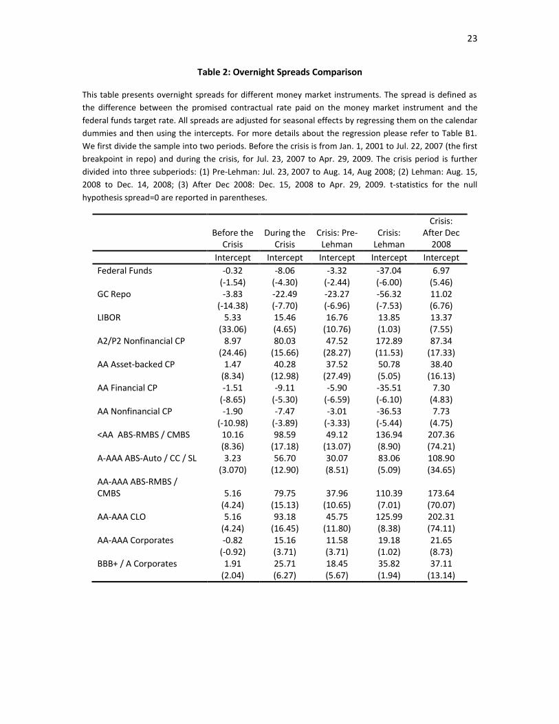
Table 2 presents the deseasonalized spreads, for different subsamples: prior to the crisis, during the
crisis, and for three different stages of the crisis (corresponding to subsequently estimated breakpoints
in the series). Table 2 allows us to see the relative ability of the private sector to produce “money.”
(Figure 1 shows these deseasonalized spreads before and during the crisis.)
Focusing first on the period prior to the crisis, the following is clear. All spreads are less than 11 bps.
Also, note that the spreads on GC repo, A1/P1 financial CP, A1/P1 nonfinancial CP are significantly
negative, that is they are below the target federal funds rate. Federal funds are unsecured, but banks
are overseen by the Fed. GC repo is collateralized by U.S. Treasuries, so it is better collateral than
federal funds, which is backed by a bank’s portfolio. And, banks are examined, that is, screened. By
screening issuers, the spreads on the highest quality CP are negative.
Relative to federal funds, it is hard for the private sector to replicate the moneyness of the best
instruments. The other money market instruments are of lower quality in that the collateral is of lower
quality or the issuers are of lower quality. Spreads on these categories are all positive, relative to the
federal funds target rate. Finally, note that LIBOR is significantly higher than federal funds. Perhaps
global banks are not screened as well as U.S. banks.
The categories with the highest spreads are repo backed by asset-backed securities with lower ratings
and A2/P2 nonfinancial commercial paper. A2/P2 is the lowest (worst) rating for commercial paper and
it had an average spread of 8.97 basis points. Also, repo which uses asset-backed securities (ABS),
residential mortgage-backed securities (RMBS), or commercial mortgage-backed securities (CMBS),
which have a rating below AA, had an average spread of 10.16 basis points.17 After these two categories
comes LIBOR with a spread of 5.33 basis points. Prior to the crisis LIBOR was widely believed to
16
The appendix does not present all the regressions behind the results in Table 2 for the sake of space. Only the results for the period prior to the crisis are presented. 17
The largest nonmortgage asset types in ABS are student loans, car loans, and credit card receivables. Subsequently, we use ABS to indicate all types of securitizations. See Gorton and Metrick (2011) for details about securitization.
8
correspond to AA risk. Next is repo with the same collateral, but rated AA or higher, at 5.16 basis points,
and collateralized loan obligations rated AA or higher which has the same spread.
What happened to the money markets in the crisis? We take as the crisis period the period following
the first breakpoint in repo (discussed below). This is the column called “During the Crisis” in Table 2.18
Note that money market instruments that are “high quality” show reduced spreads. These include
federal funds, general collateral repo, and A1/P1 commercial paper, both financial and nonfinancial.19
This is the flight to quality, where some instruments are perceived as better money. But, all the other
money market instruments’ spreads show very large increases. Figure 1 displays the spreads (intercepts)
before and during the crisis.
The other instruments, all privately-produced, show large spikes in their spreads; see Figure 1. For
example, repo backed by residential mortgage-backed securities or commercial mortgage-backed
securities, rated lower than AA, increase from 10.16 to an average of 98.59 basis points during the crisis.
A1/P1 asset-backed CP rises from an average of 1.5 basis points in normal times to 40.28 basis points
during the crisis.
The table also shows the results for subperiods during the crisis corresponding to the other breakpoints.
The subperiods are (1) Pre-Lehman: the crisis from the onset to Lehman (the second breakpoint in repo
discussed below); (2) Lehman: the aftermath of Lehman until December 2008; and (3) After December
2008. The middle period of the crisis, which brackets the failure of Lehman Brothers, was the height of
the crisis in terms of spreads. After December 2008, spreads are lower than in the Lehman period,
except for all categories of repo using asset-backed securities as collateral. The spreads on repo backed
by ABS just kept rising. ABS (including RMBS and CMBS) becomes “information-sensitive” (in the
nomenclature of Dang, Gorton and Holmström (2011)) and can’t be used as collateral. See Gorton and
Metrick (2012).
Figure 2 conveys a sense of what happened in the crisis. Figure 2 shows the spreads adjusted for the
seasonal effects. The two vertical lines in the figure correspond to two of the breaks in the set of repo
spreads (that we discuss shortly). Before the first break in repo, early in 2007, the spreads are tightly
bunched, with the occasional uptick. There are two crisis regimes visible: the Crisis and Run phases. The
18
As before, the table shows spreads calculated with regressions including the calendar dummies, like the previous results in Appendix Table A1. To save space though these results are not included. 19
The spread for fed funds is the average difference between the effective fed funds rate and the target rate.

9
first occurs around August 2007 and last until the second repo break. The second starts with the Lehman
bankruptcy. As we saw before, in Table 2, not all spreads widen. Spreads diverge as some instruments
lose their moneyness (become risky) and others become a safe haven.
4. Understanding the Dynamics of the Crisis: A Chronology
I this section we turn to a formal statistical chronology of the recent financial crisis.
A. Breakpoints Methodology
To produce a chronology of the financial crisis we need to find random but common breakpoints in a
panels. We estimate breakpoints in different panel data sets, where each panel has a recognizable
economic meaning whereas most studies of breakpoints focus on a single series, treating series
separately.20
For our study, basing the breakpoints on panel data is important. A definition of a financial crisis is that
it is a common breakpoint in many money and banking time series at the same time. And a crisis is then
followed by real effects. The econometric procedure formalizes this.
Also, it is possible to consistently estimate breakpoints using a panel, while there may be little or no
power to looking at individual time series when there is not much data covering the crisis regime. In
other words, in a univariate setting there may be little hope of detecting a regime switch when a single
observation that may be an outlier can have a large effect on the estimate, or when one regime consists
of only a few observations in time. In our setting the crisis period is relatively short and comes at the
end of the sample.
We follow the estimation approach of Bai (2010). Briefly, the idea is to consider a panel of N series, as
follows:
Yit = μi1 + σi1ηit, t = 1,2, . . . , k0
Yit = μi2 + σi1ηit,, t = k0+1, . . . T
20
There is a large literature on change point estimation for univariate series and only a small but emerging literature on estimating common breakpoints in panel data. On breakpoint estimation in general, see Perron (2005) and Hansen (2001). Bai (2010) provides the references to the other papers on the estimation of breakpoints in panels.

10
i = 1,2, . . . , N
where E(ηit)=0 and var(ηit)=1, and for each i, ηit is a linear process; there are other assumptions as well;
see Bai (2010). The breakpoint, k0 in means and variances is unknown. Consistent estimation requires
that there are breakpoints in either the means or the variances (or both). Assuming a common
breakpoint is more restrictive than assuming random breakpoints in the different series in the panel.
But, the assumption results in more precise estimation. The basic idea of Bai’s approach is to exploit the
cross-section information, sort of “borrowed power” relative to the non-panel approach.
The breakpoint is estimated with quasi-maximum likelihood (QML). Let
�̂�𝑖12 (𝑘) =
1
𝑘∑ (𝑌𝑖𝑡 − �̅�𝑖1
𝑘𝑡=1 )2, �̂�𝑖2
2 (𝑘) =1
𝑇−𝑘∑ (𝑌𝑖𝑡 − �̅�𝑖2
𝑇𝑡=𝑘+1 )2.
The QML objective function for series i is:
𝑘 𝑙𝑜𝑔 �̂�𝑖12 (𝑘) + (𝑇 − 𝑘)𝑙𝑜𝑔 �̂�𝑖2
2 (𝑘),
multiplied by one half. Analogously, for N series:
𝑈𝑁𝑇(𝑘) = 𝑘 ∑ 𝑙𝑜𝑔 �̂�𝑖12 (𝑘)𝑁
𝑖=1 + (𝑇 − 𝑘) ∑ 𝑙𝑜𝑔𝑁𝑖=1 �̂�𝑖2
2 (𝑘).
The breakpoint estimator is �̂� = 𝑎𝑟𝑔𝑚𝑖𝑛𝑘𝑈𝑁𝑇(𝑘). Bai (2010) Theorem 5.1 shows that the breakpoint in
this case can be consistently estimated.21
We next build on the chronology by looking at subsequent break points.22 See Appendix B.
Our approach is to group the data series into five different panels with recognizable economic content:
(1) the real sector of the economy; (2) the subprime housing sector; (3) financial firms; (4) the unsecured
21 Note that we are not testing sudden breaks against the alternative hypothesis of gradual or smooth structural
changes. Chen and Hong (2012), for example, propose a test for smooth structural changes in time series, but not panels. The Bai procedure and the tests for smooth changes both test against the alternative of no change, and we cannot test to determine whether the change is sudden or gradual. 22 Bai (2010): “Once the first break is obtained, we split the sample at the estimated break point, resulting in two
subsamples. We then estimate a single break point in each of the subsamples, but only one of them is retained as our second estimator. The one that gives a larger reduction in the sum of squared residuals is kept.” (p. 86)

11
money markets; and (5) the secured money markets. We further divide the financial firms to consider
including and excluding Lehman. We also consider subsets of the real sector and subprime.23
The real sector is represented by the S&P 500 index return, the VIX index (the Chicago Board Options
Exchange Market Volatility Index), the JP Morgan High Yield Bond Index, and the Dow Jones CDX.IG
index of investment grade credit derivative premia. The subprime sector is represented by the spreads
on tranches of the ABX index (an index of derivative premia linked to subprime bonds), and two series of
subprime bond spreads. The financial sector is represented by the CDS premia on ten banks, including
Lehman Brothers (see Table 1). Finally, there are the returns on thirteen money market instruments,
including four categories of commercial paper, fed funds, LIBOR, and the rates on seven categories of
repo, including general collateral. The returns on the money market instruments are annualized
overnight returns. We split the money market instruments into secured (repo), unsecured, and GC repo.
Later, we also look at some individual money market series.
After the first breakpoint is found, the subsequent breakpoints in each panel are (almost always) during
the crisis period. But, these breakpoints are not necessarily chronologically ordered. So, chronologically
the second breakpoint may come after the third breakpoint. Appendix B provides more information on
the ordering of the breakpoints using the Bai procedure versus the chronological ordering. In what
follows we show the breakpoints chronologically. The issue of the order in which the breakpoints are
found and the chronological ordering not matching is discussed later and in Appendix B.
B. Spreads
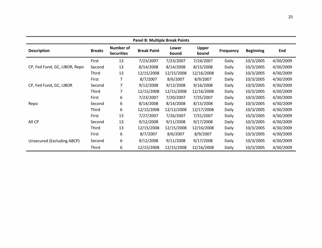
We first focus on spreads and ask how the crisis evolved. Table 3 addresses this question. Table 3, Panel
A, provides the breakpoints located for the different panel data sets shown in the table. The table also
provides 99 percent confidence intervals for the breakpoints in terms of dates. The main results are as
follows.
The subprime shock occurs in the first quarter of 2007, on January 4, 2007. If we look only at the ABX
tranches then the break occurs on January 25, 2007. If we only look at the two subprime series, the
break is March 22, 2007. This timing is consistent with the failures of a number of subprime originators
and the downgrades of subprime bonds by the rating agencies. See the chronology in Gorton (2010).
23
In terms of the number of series in a panel, precision is improved with a larger number of series. Clearly, the confidence intervals depend on N. But, as a practical matter N can also be small. Bai (2010) provides a sense of the precision with Monte Carlo experiments where the number of series, N, in the panel ranges from one to 100.

12
The next breakpoint occurs in the repo market on July 23, 2007. This is also when the breakpoint for the
dealer banks’ CDS occurs, whether we include Lehman or not. This is the start of the financial crisis,
although as we will see subsequently haircuts do not rise until later. The breakpoints here confirm the
start in the sense that the breakpoint for the repo spreads and for the dealer bank CDS premia is the
same date. This is not surprising as the rise in repo spreads suggests that this form of financing is
becoming riskier, raising the possibility of a run.
In untabulated results, we also looked at thirteen categories of non-mortgage ABS spreads. These
spreads show a first break on July 19, 2007, with the 99% confidence interval of July 19, 2007-July 26,
2007. We also looked at the CDS premia of thirteen European banks; these show a first break on July
25, 2007.24 The standard error shows a lower bound of July 23, 2007. So, the breakpoints overlap with
the start of the crisis in the U.S. consistent with Dang, Gorton and Holmström (2014) who argue that a
crisis is an information event corresponding to a shift from information-insensitive to information-
sensitive for broad categories of asset classes—all securitizations! In this sense, there was no
“contagion” from subprime to other securitization asset classes. Since European banks were also
involved in securitization, as holders of these bonds, they too were affected.
The unsecured money market instruments, CP, fed funds, and LIBOR, show a breakpoint on August 8,
2007. Note that the 99 percent confidence intervals for the secured and unsecured money market
instruments statistically distinguish the two dates for the repo markets and the unsecured money
markets. There is a difference between the secured and unsecured markets. Repo is collateralized by a
single bond, whereas unsecured instruments are backed by portfolios.25
The crisis, starting in the third quarter of 2007, only begins to affect the real sector later. The real
sector, measured by the VIX, and the returns on the S&P500, the JPM HY Index, and the DJ CDX.IG,
shows a break on January 3, 2008. The NBER dates the start of the recession in December 2007. If we
separate the equity-related series from the bond-related series and only look at the VIX and the S&P,
then the break is September 12, 2008 –nine months later. Lehman Brothers’ failed on September 15,
2008, within the 99 percent confidence interval for the break in this latter case. The Troubled Asset
Relief Program (TARP) became law on October 3, 2008.
24
The banks included were Credit Agricole Group, BNP Paribas, Deutsche Bank, Barclays, Royal Bank of Scotland, Societe Generale, Banco Santander, Lloyds, UBS, UnitCredit, Credit Suisse and Rabobank. 25
Keep in mind also that if a counterparty goes bankrupt, this does not affect ownership of the repo collateral, but CP holders must go into the bankruptcy process to try to recover their loan.

13
In Table 4 we look at two single series, as one might expect that ABCP and GC repo spreads to behave
differently. Indeed, ABCP by itself shows a break July 27, 2007, and the 99 percent confidence interval
overlaps with the first break for repo. This is consistent with the run on ABCP, which resulted in banks
taking conduit assets back via liquidity facilities, and then financing this at least in part via repo. Also,
note that when looking at GC repo as a single series, there is a break on August 13, 2007. This is likely
the flight to quality by investors with cash since they did not roll their ABCP.
C. Repo Haircuts
In this subsection we look at repo haircuts. As discussed in Gorton (2010) and Gorton and Metrick
(2012), increasing repo haircuts corresponds to withdrawing cash from the banking system. For
example, suppose a lender in the repo market deposits $100 million overnight at interest. To keep the
deposit safe the bank provides $100 million of bonds (valued at market prices). The depositor takes
possession of these bonds. The next morning suppose the borrower wants to renew or roll the repo. If
the lender is nervous, he may offer to lend $90 million but wants to keep the $100 million of bonds at
collateral (getting $10 million dollars of cash back from the borrower). This is called a 10 percent haircut.
It corresponds to a withdrawal of $10 million from the bank because now the bank has to finance this
amount from other sources.
Table 5 shows the breakpoints in haircuts in the panel of the six categories of repo that use
privatelyproduced collateral. The pattern of breakpoints in the haircuts is quite remarkable. The first
repo haircut breakpoint occurs on October 23, 2007, after the breaks in the spreads in the first cluster.
The second breakpoint occurs on February 6, 2008, right around the time that the real effects of the
crisis are felt. Not surprisingly, the third breakpoint is September 15, 2008, the day of Lehman’s failure.
D. Financial Firms: Credit Derivative Premia
The break in repo spreads in July means that the short-term funding of dealer banks is under pressure.
How significant was this pressure and when was the onset? To examine this, the most relevant asset
prices to look at are credit default swaps (CDS) referencing the dealer banks. We find that dealer bank
spreads show a breakpoint at the same date that repo and ABCP show their first breaks.
Table 6 shows the breakpoints for the five year CDS on the nine financial firms listed in Table 1, with
Lehman and without Lehman. The first break in financial CDS is coincident with the first break in repo
spreads and the first break in ABCP spreads. The second break occurs on February 8, 2008. This is a few

14
days before President Bush signed the Economic Stimulus Act of 2008 on February 13, 2008, and before
JP Morgan purchased Bear Stearns, on March 16, 2008.
The third break is on September 11, 2008. It is prior to the Lehman failure on September 15, 2008,
consistent with Gorton, Metrick and Xie (2015) who argue that this corresponds to a buildup of fragility
during the crisis. This is also reflected in the CDS spreads.
5. The Crisis Chronology
Our findings are summarized in Figure 3. Figure 3 lists (almost) all of the breakpoints discussed above,
and also include some other major public events for reference to the other narrative.
The subprime shock occurs on January 4, 2007. Repo spreads and ABCP spreads both respond in late
July 2007, the same time that dealer banks are shocked. On August 7, 2007, the other money market
instruments are affected. Their spreads spike. Lastly, repo haircuts significantly increase on October 23,
2007. Finally, the real economy is affected starting on January 3, 2008. The crisis then evolves. Repo
haircuts show a second breakpoint February 6, 2008, putting the financial firms at greater risk; their CDS
shows a second break two days later, on February 8, 2008, reflecting this. JP Morgan buys Bear Stearns
on March 16, 2008.
Further, still prior to Lehman, on August 14, 2008, repo spreads have a break. September 11, 2008
there is another break in the financial firms’ CDS. Unsecured money market instruments’ spreads have
breaks on September 12, 2008. The buildup culminates in the collapse of Lehman on September 15,
2008. Repo haircuts going up in this case is the run on Lehman. The break is the same day.
6. Conclusion
What do we learn from this econometric approach? First, in terms of what a crisis is, we find that not
only repo and ABCP show breaks at the same time, but that coincident with this date, the credit
derivative premia of the banks show a break. This suggests their problems were due to the
deteriorating repo and ABCP markets. Dang, Gorton and Holmström (2011) argue short-term debt is
useful for trading and storing value over short intervals because it is designed to immune to private
information production by agents; it is information-insensitive. A “crisis” is a situation where
lenders/depositors fear that they face adverse selection when using short term debt. This debt which
was previously information-insensitive has become information-sensitive (i.e. due to a public signal
some agents have an incentive to become privately informed about the collateral backing the bank debt.

15
In the case of repo and ABCP, the backing collateral was often non-mortgage asset-backed securities.
Consistent with Dang, Gorton, and Holmström (2011), we find the break in the spreads on thirteen non-
mortgage ABS at the same time as repo, ABCP, and financial firm CDS.
Second, we learn that the crisis involved subsequent dynamics shown by further breakpoints. This
suggests that fragility was building up before the Lehman collapse, consistent with the shortening of
maturities of money market instruments during the crisis, found by Gorton, Metrick and Xie (2015). This
suggests that systemic risk is endogenous and cannot necessarily be detected prior to the onset of a
crisis

16
Appendix A: Seasonals in Money Market Spreads
In this appendix we briefly discuss the calendar effects or “seasonals” in money market spreads.
Appendix Table B1 shows regressions of the money markets spreads on calendar dummies, and shows
that “seasonals” are important in money market spreads. There are spikes in many of the spreads at
certain calendar dates. Just before the quarter end (five days before to the day before) and the date of
the quarter-end and day after, show the largest increases. But, note that the largest increases on those
dates are in the repo markets. Repo using all categories of private securities as collateral show
significant spikes in spreads around the quarter-end. For example, repo that uses collateralized loan
obligation tranches rates AA-AAA spikes by 77 basis points the day of the quarter-end and the next day.
Repo backed by asset-backed securities composed of auto loans, credit card receivables, or student
loans rated AA-AAA also spikes by 71 basis points on those days. Unsecured money market instruments
show much lower increases on those dates. For example, LIBOR goes up 4 basis points, A1/P1 Financial
CP goes up by 8 basis points, and A1/P1 asset-backed commercial paper goes up by 9 basis points.
There is more seasonal pressure on repo markets. A seasonal increase in the spread in repo suggests
that borrowers are willing to pay more for cash at these seasonal dates than at other dates to finance
the collateral. But, the depositors/lenders, on the other hand, appear to want their cash (and not the
collateral) at these dates.
Why is there a large demand for cash at these dates? Large movements of cash which go from one
party to another, especially if one party is the government so cash leaves the economy, could cause
these spikes in spreads. In the period before the Federal Reserve System there were seasonal spikes in
interest rates when cash had to move from cities to rural areas for planting season and then later for
harvesting season. Indeed, such spikes were viewed as creating fragility in the system and were a major
motivation for the founding of the Federal Reserve System.26
In the modern era since the founding of the Federal Reserve System there are several possible
candidates for explaining seasonals. One candidate for large cash movements is the payment of
estimated taxes by corporations. Another possibility is quarter-end “window dressing,” which might
show up for example in the excess reserves of banks, if they are engaged in window dressing.
26
On seasonals in the money markets prior to the Fed see Kemmerer (1911). On seasonals and fragility prior to the Fed see Miron (1986). And, on the elimination of some of the seasonals in interest rates once the Fed comes into existence, see Mankiw, Miron and Weil (1987).
17
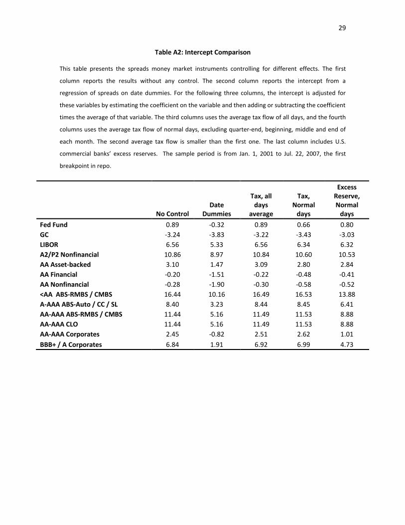
We examine these issues in Table B2. The table contains the intercepts on each money market
instrument with no controls, in the first column, and also with the date dummies from Table B1, in the
second column. The next two columns show the change in the intercept when two tax variables are
(separately) used in the panel regression. The two variables are the same. In both columns, we report
the fitted values. We first estimate the parameters for tax flow process. Then we use the average tax
flow to replace the actual tax flow and calculate the fitted value. For the variable “Tax, all days
average”, we assume tax flow equals the average tax flow across all days. For the variable “Tax, Normal
days”, we assume that tax flow equals the average tax flow across normal days, excluding quarter-end,
beginning, middle and end of each month. The second average tax flow is smaller than the first one.
The last column includes U.S. commercial banks’ excess reserves. The intercept is adjusted for these
variables by estimating the coefficient on the variable and then adding or subtracting the coefficient
times the average of that variable. So, for example, in column 3 the coefficient times the average inflow
of taxes to the government, averaged over all (business) days, shows no effect, as the intercepts change
very little. When the middle of the month is excluded, the intercept does go down in most cases, but
not by much.
Inclusion of the excess reserves variable does reduce the intercept for repo categories, but not by as
much as the calendar dummies that we started with.
These calendar effects are a subject for future research.

18
Appendix B: Chronology Breakpoints
In this appendix we briefly discuss the ordering of breakpoints.
As explained briefly in the main text, the Bai procedure finds a breakpoint for the given panel. The
second breakpoint looks at the two subperiods defined by the first breakpoint and minimizes the sum of
squared residuals over the whole sample using QML. The second breakpoint we find is usually after the
date of the first breakpoint, but need not be. This means that we do not condition on the first
breakpoint. In other words, the second breakpoint could be before the first breakpoint. Similarly, the
third breakpoint is determined by looking at the ALL the subperiods determined by the first and second
breakpoints.
The issues are illustrated by Figure C1, which shows two possible Bai orderings. The first breakpoint in
both panels, A and B, is the crisis date. This is true in the data. In Panel A, the first three breakpoints
occur at the crisis date and then chronologically in order. But, breakpoint four is before the crisis date.
In general we are only interested in the first three breakpoints. However, we always calculate the
fourth breakpoint because sometimes the ordering looks more like what is shown in Panel B.
In Panel B, the fourth breakpoint occurs during the crisis, and comes before the second breakpoint. But,
the third breakpoint is before the crisis onset.
In order to understand the sensitivity of the procedure, particularly given the seasonals, we show the
ordering according to the Bai algorithm and the chronological ordering. Table B1 provides examples for
the most important panels. It illustrates the differences between the breakpoints found by the Bai
algorithm and the chronological ordering of the breakpoints. In the table “Algorithm Order” equal 1
means that is the first breakpoint fund by the Bai procedure. “Chronological Order” means that after we
found four breakpoints we sorted them chronologically and labeled them 1 through 4.
These issues are shown in Table C1.

19
References
Acharya, Viral, Philipp Schnabl, and Gustavo Suarez (2011), “Securitization without Risk Transfer,”
Journal of Financial Economics 107, 515-536.
Allen, Linda and Anthony Saunders (1992), “Bank Window Dressing: Theory and Evidence,” Journal of
Banking and Finance 16, 585-623.
Bai, Jushan (2010), “Common Breaks in Means and Variances for Panel Data,” Journal of Econometrics
157, 78-92.
Boyd, John, Gianni De Nicolò, and Elena Loukoianova (2011), “Banking Crises and Crisis Dating: Theory
and Evidence,” International Monetary Fund, working paper.
Calomiris, C.W., (1994), “Is the Discount Window Necessary: A Penn-Central Perspective,” Federal
Reserve Bank of St. Louis Review, 76, 31-56.
Calomiris, C.W., (1989), “The Motivations for Loan Commitments Backing Commercial Paper,” Journal of
Banking and Finance 1, 271-77.
Calomiris, Charles, Charles Himmelberg, and Paul Wachtel (1995), “Commercial Paper, Corporate
Finance, and the Business Cycle: A Microeconomic Perspective,” Carnegie-Rochester Conference
Series on Public Policy 42, 203-250.
Caprio, Gerard and Daniela Klingebiel (1996), “Bank Insolvencies: Cross-Country Experience,” World
Bank Policy Research Working paper PRWP1620.
Caprio, Gerard and Daniela Klingebiel (1999), “Episodes of Systemic and Borderline Financial Crises,”
World Bank, working paper.
Chen, Bin and Yongmiao Hong (2012), “Testing for Smooth Structural Changes in Time Series Models via
Nonparametric Regression,” Econometrica 80, 1157-1183.
Covitz, Daniel M., Nellie Liang, and Gustavo A. Suarez (2012), "The Evolution of a Financial Crisis:
Collapse of the Asset-Backed Commercial Paper Market," Journal of Finance 68, 815-848.
Crabbe, Leland and Mitchell Post (1994), “The Effect of a Rating Downgrade on Outstanding Commercial
Paper,” Journal of Finance 49, 39-56.
Dang, Tri Vi, Gary Gorton and Bengt Holmström (2011), “Financial Crises and the Optimality of Debt for
Liquidity Provision.”
Demirgϋç-Kunt, Asli and Enrica Detrachiache (2002), “Does Deposit Insurance Increase Banking System
Stability? An Empirical Investigation,” Journal of Monetary Economics 49, 1373-1406.

20
Demirgϋç-Kunt, Asli and Enrica Detrachiache (2005), “Cross-Country Empirical Studies of Systemic Bank
Distress: A Survey,” National Institute Economic Review, No. 192, April.
Fender, Ingo and Martin Scheicher (2008), “The ABX: How Do the Markets Price Subprime Mortgage
Risk?,” BIS Quarterly Review (September), 67-81.
Fitch Ratings (2007), “Asset-Backed Commercial Paper & Global Banks Exposure—10 Key Questions,”
Special Report (September 12, 2007).
Fons, Jerome and Andrew Kimball (1991), “Defaults and Orderly Exits of Commercial Paper Issuers,
1972-1990,” Moody’s Special Report (January).
Gorton, Gary (2010), Slapped by the Invisible Hand: The Panic of 2007 (Oxford University Press).
Gorton, Gary and Andrew Metrick (2012), “Securitized Banking and the Run on Repo,” Journal of
Financial Economics 104, 425-451.
Gorton, Gary and Andrew Metrick (2011), “Securitization,” chapter in the Handbook of the Economics of
Finance, volume 2, edited by George Constantinides, Milton Harris, and René Stulz, Elsevier,
forthcoming.
Gorton, Gary, Andrew Metrick and Lei Xie (2015), “The Flight from Maturity,” working paper.
Griffiths, Mark and Drew Winters (2005), “The Turn of the Year Money Markets: Tests of the Risk-Shifting
Window Dressing and Preferred Habitat Hypothesis,” Journal of Business 78, 1337-1363.
Hansen, Bruce (2001), “The New Econometrics of Structural Change: Dating Breaks in U.S. Labor
Productivity,” Journal of Economic Perspectives 15, 117-128.
He, Zhiguo, Ingu Khang, and Arvind Krishnamurthy (2010), “Balance Sheet Adjustment in the 2008 Crisis,”
IMF Economic Review 58, 118-156.
Iyer, Rajkamal and Manju Puri (2012), “Understanding Bank Runs: The Importance of Depositor-Bank
Relationships,” American Economic Review 102(4), 1414-1445.
Kelly, Morgan and Cormac Ó Gráda (2000), “Market Contagion: Evidence from the Panics of 1854 and
1857,” American Economic Review 90(5), 1110-1124.
Kemmerer, E. W. (1911), “Seasonal Variation in the New York Money Market,” American Economic Review
1, 33-49.
Komotin, Vladimir and Drew Winters (2006), “Quarter-End Effects in Banks: Preferred Habitat or Window
Dressing?,” Journal of Financial Services Research 29, 61-82.
Krishnamurthy, Arvind, Stefan Nagel, and Dmitry Orlov (2014), “Sizing Up Repo,” Journal of Finance 70.

21
Mankiw, N. Gregory, Jeffrey Miron, and David Weil (1987), “The Adjustment of Expectations to a Change in
Regime: A Study of the Founding of the Federal Reserve,” American Economic Review 77, 358-
374.
McCabe, Patrick (2010), “The Cross Section of Money Market Fund Risks and Financial Crises,” Federal
Reserve Board, working paper no. 2010-51.
Miron, Jeffrey (1986), “Financial Panics, the Seasonality of the Nominal Interest Rate and the Founding of
the Fed,” American Economic Review 76, 125-140.
Moody’s Investors Services (2007), “Moody’s Update on Bank-Sponsored ABCP Programs: A Review of
Credit and Liquidity Issues,” International Structured Finance, Special Report (September 12,
2007).
Moody’s Investors Services (2003), “The Fundamentals of Asset-Backed Commercial Paper,” Structured
Finance, Special Report (February 3, 2003).
Musto, David (1997), “Portfolio Disclosures and Year-End Price Shifts,” Journal of Finance 52, 1861-82.
Nayar, Nandkumar, and Michael S. Rozeff (1994), “Ratings, Commercial Paper, and Equity Returns,”
Journal of Finance 49, 1431-1449.
Ó Gráda, Cormac, and Eugene White (2003), “The Panics of 1854 and 1857: A View from the Emigrant
Industrial Savings Bank,” Journal of Economic History 63 (1), 213–40.
Perron, Pierre (2006), “Dealing with Structural Breaks,” chapter in Palgrave Handbook of Econometrics,
Volume 1, edited by Terence Mills and Kerry Patterson (Palgrave Macmillan), 278-352.
Reinhart, Carmen, and Kenneth Rogoff (2008), “Banking Crises: An Equal Opportunity Menace,” NBER
Working Paper 14587.
Sprague, O. M. W. (1910), History of Crises under the National Banking System, Senate Document 538
(Washington DC: Government Printing Office).
Wessel, David (2010), In Fed We Trust: Ben Bernanke’s War on the Great Panic (Crown Business).

Table 1: Data Sources and Sample Periods
This table summarizes the data used in the paper. Their sources, sample periods and short descriptions are presented.
Variable Source Sample Periods
Description Beginning End
VIX CBOE 1/1/2000 4/30/2009 CBOE Volatility Index
S&P 500 Standard & Poor's 1/1/2000 4/30/2009 Standard & Poor's 500 Index return
JPM HY Index Dealer Bank 4/10/2003 4/30/2009 J.P. Morgan High Yield Index
DJ CDX.IG Dealer Bank 4/10/2003 4/30/2009 Dow Jones CDX Index (Investment grade)
ABX Dealer Bank 1/19/2006 4/30/2009 Markit ABX.HE Index, 2006-1. AAA, BBB and BBB-
HEL Dealer Bank 1/19/2006 1/3/2008 Home Equity Loan ABS spreads, AAA and BBB ratings
Financial CDS Bloomberg 11/6/2002 4/30/2009 5 Year CDS for Bank of America, JP Morgan, Citigroup, Wells Fargo, Wachovia, Goldman Sachs, Merrill Lynch, Morgan Stanley, Lehman Brother and Bear Stearns.
Interbank Money Markets
Fed Fund Bloomberg 12/20/2001 4/30/2009 Effective Federal Fund rate
LIBOR Bloomberg 12/20/2001 4/30/2009 LIBOR
OIS Bloomberg 12/20/2001 4/30/2009 Overnight indexed swap
Commercial Paper
A2/P2 Nonfinancial Federal Reserve 12/20/2001 4/30/2009 SIC code: 100-5999, 7000-9999. Programs with at least one "2" rating but no ratings other than "2"
AA Asset-backed Federal Reserve 12/20/2001 4/30/2009 SIC code: 6189. Programs with at least one "1" or "1+" rating but no ratings other than "1"
AA Financial Federal Reserve 12/20/2001 4/30/2009 SIC code: 6000-6999, excluding 6189. Programs with at least one "1" or "1+" rating but no ratings other than "1"
AA Nonfinancial Federal Reserve 12/20/2001 4/30/2009 SIC code: 100-5999, 7000-9999. Programs with at least one "1" or "1+" rating but no ratings other than "1"
Repo Categories
GC Bloomberg 12/20/2001 4/30/2009 General collateral repo rate
<AA ABS-RMBS / CMBS Dealer Bank 10/3/2005 4/30/2009 Residential mortgage-backed security (RMBS) or commercial mortgage-backed security (CMBS) with ratings less than AA
A-AAA ABS-Auto / CC / SL Dealer Bank 10/3/2005 4/30/2009 Asset-backed securities (ABS) comprised of auto loans, credit-card receivables, or student loans, with ratings between A and AAA, inclusive.
AA-AAA ABS-RMBS / CMBS
Dealer Bank 10/3/2005 4/30/2009 Residential mortgage-backed security (RMBS) or commercial mortgage-backed security (CMBS) with ratings between AA and AAA, inclusive.
AA-AAA CLO Dealer Bank 10/3/2005 4/30/2009 Collateralized loan obligations (CDO) with ratings between AA and AAA, inclusive.
AA-AAA Corporates Dealer Bank 10/3/2005 4/30/2009 Corporate bonds rated between AA and AAA, inclusive.
BBB+ / A Corporates Dealer Bank 10/3/2005 4/30/2009 Corporate bonds rated between BBB+ and A, inclusive.
23
Table 2: Overnight Spreads Comparison
This table presents overnight spreads for different money market instruments. The spread is defined as
the difference between the promised contractual rate paid on the money market instrument and the
federal funds target rate. All spreads are adjusted for seasonal effects by regressing them on the calendar
dummies and then using the intercepts. For more details about the regression please refer to Table B1.
We first divide the sample into two periods. Before the crisis is from Jan. 1, 2001 to Jul. 22, 2007 (the first
breakpoint in repo) and during the crisis, for Jul. 23, 2007 to Apr. 29, 2009. The crisis period is further
divided into three subperiods: (1) Pre-Lehman: Jul. 23, 2007 to Aug. 14, Aug 2008; (2) Lehman: Aug. 15,
2008 to Dec. 14, 2008; (3) After Dec 2008: Dec. 15, 2008 to Apr. 29, 2009. t-statistics for the null
hypothesis spread=0 are reported in parentheses.
Before the
Crisis During the
Crisis Crisis: Pre-
Lehman Crisis:
Lehman
Crisis: After Dec
2008
Intercept Intercept Intercept Intercept Intercept
Federal Funds -0.32 -8.06 -3.32 -37.04 6.97
(-1.54) (-4.30) (-2.44) (-6.00) (5.46)
GC Repo -3.83 -22.49 -23.27 -56.32 11.02
(-14.38) (-7.70) (-6.96) (-7.53) (6.76)
LIBOR 5.33 15.46 16.76 13.85 13.37
(33.06) (4.65) (10.76) (1.03) (7.55)
A2/P2 Nonfinancial CP 8.97 80.03 47.52 172.89 87.34
(24.46) (15.66) (28.27) (11.53) (17.33)
AA Asset-backed CP 1.47 40.28 37.52 50.78 38.40
(8.34) (12.98) (27.49) (5.05) (16.13)
AA Financial CP -1.51 -9.11 -5.90 -35.51 7.30
(-8.65) (-5.30) (-6.59) (-6.10) (4.83)
AA Nonfinancial CP -1.90 -7.47 -3.01 -36.53 7.73
(-10.98) (-3.89) (-3.33) (-5.44) (4.75)
<AA ABS-RMBS / CMBS 10.16 98.59 49.12 136.94 207.36
(8.36) (17.18) (13.07) (8.90) (74.21)
A-AAA ABS-Auto / CC / SL 3.23 56.70 30.07 83.06 108.90
(3.070) (12.90) (8.51) (5.09) (34.65)
AA-AAA ABS-RMBS / CMBS 5.16 79.75 37.96 110.39 173.64
(4.24) (15.13) (10.65) (7.01) (70.07)
AA-AAA CLO 5.16 93.18 45.75 125.99 202.31
(4.24) (16.45) (11.80) (8.38) (74.11)
AA-AAA Corporates -0.82 15.16 11.58 19.18 21.65
(-0.92) (3.71) (3.71) (1.02) (8.73)
BBB+ / A Corporates 1.91 25.71 18.45 35.82 37.11 (2.04) (6.27) (5.67) (1.94) (13.14)

24
Table 3: Crisis Chronology
This table presents the common breakpoints following Bai’s (2010) procedure for different groups of data. Panel A shows the first breakpoints and the lower
and upper bound of their 99% confidence intervals. The number of securities, the data frequency and the sample period for each group are also reported.
Panel B shows the second and third breakpoints in the money market spreads data. Financial CDS include the 5-year credit default swaps (CDS) on 10 top U.S.
financial institutions, including commercial banks and dealer banks. The list of banks is in Table 1. CP includes four categories of commercial paper: A2/P2
nonfinancial, A1/P1 asset-backed commercial paper, A1/P1 financial, and A1/P1 nonfinancial. Repo include six categories of repo, which differ by the type of
privately-produced collateral used as backing: AAA/Aaa-AA/Aa asset-backed securities (ABS), including residential mortgage-backed (RMBS) and commercial
mortgage-backed securities (CMBS), RMBS and CMBS with ratings between AA and AAA , AAA/Aaa-A/A auto loan-backed, credit card receivables-backed and
student loan-backed ABS, AAA/Aaa-AA/Aa collateralized loan obligations (CLOs), AAA/Aaa-AA/Aa corporate bonds, and A/A-Baa/BBB+ corporate bonds.
Panel A: Common Break Points
Description Num. of Securities
Break Point
Lower bound
Upper bound Frequency Beginning End
Real Sector: VIX and S&P 500 2 2008/9/12 2008/9/12 2008/9/15 Daily 2000/1/1 2009/4/30 Real Sector: VIX, S&P 500, JPM HY Index, DJ CDX.IG 6 2008/1/3 2008/1/3 2008/1/10 Weekly 2003/4/10 2009/4/30 Subprime: ABX only 3 2007/1/25 2007/1/24 2007/1/29 Daily 2006/1/19 2009/4/30 Subprime: HEL only 2 2007/3/22 2007/3/22 2007/3/29 Weekly 2006/1/19 2008/1/3 Subprime: ABX & HEL 5 2007/1/4 2007/1/4 2007/1/11 Weekly 2006/1/19 2008/1/3 Financial CDS: Include Lehman 10 2007/7/10 2007/7/10 2007/7/11 Daily 2007/1/1 2008/9/12 Financial CDS: Exclude Lehman 9 2007/7/16 2007/7/16 2007/7/17 Daily 2007/1/1 2009/4/30 Money Market: CP, Fed Fund, GC, LIBOR, Repo 13 2007/7/23 2007/7/23 2007/7/24 Daily 2005/10/3 2009/4/30 Money Market: Repo 6 2007/7/23 2007/7/20 2007/7/25 Daily 2005/10/3 2009/4/30 Money Market: CP, Fed Fund, GC, LIBOR 7 2007/8/8 2007/8/8 2007/8/9 Daily 2005/10/3 2009/4/30
25
Panel B: Multiple Break Points
Description Breaks Number of Securities
Break Point Lower bound
Upper bound
Frequency Beginning End
CP, Fed Fund, GC, LIBOR, Repo
First 13 7/23/2007 7/23/2007 7/24/2007 Daily 10/3/2005 4/30/2009
Second 13 8/14/2008 8/14/2008 8/15/2008 Daily 10/3/2005 4/30/2009
Third 13 12/15/2008 12/15/2008 12/16/2008 Daily 10/3/2005 4/30/2009
CP, Fed Fund, GC, LIBOR
First 7 8/7/2007 8/6/2007 8/9/2007 Daily 10/3/2005 4/30/2009
Second 7 9/12/2008 9/12/2008 9/16/2008 Daily 10/3/2005 4/30/2009
Third 7 12/15/2008 12/15/2008 12/16/2008 Daily 10/3/2005 4/30/2009
Repo
First 6 7/23/2007 7/20/2007 7/25/2007 Daily 10/3/2005 4/30/2009
Second 6 8/14/2008 8/14/2008 8/15/2008 Daily 10/3/2005 4/30/2009
Third 6 12/15/2008 12/12/2008 12/17/2008 Daily 10/3/2005 4/30/2009
All CP
First 13 7/27/2007 7/26/2007 7/31/2007 Daily 10/3/2005 4/30/2009
Second 13 9/12/2008 9/11/2008 9/17/2008 Daily 10/3/2005 4/30/2009
Third 13 12/15/2008 12/15/2008 12/16/2008 Daily 10/3/2005 4/30/2009
Unsecured (Excluding ABCP)
First 6 8/7/2007 8/6/2007 8/9/2007 Daily 10/3/2005 4/30/2009
Second 6 9/12/2008 9/11/2008 9/17/2008 Daily 10/3/2005 4/30/2009
Third 6 12/15/2008 12/15/2008 12/16/2008 Daily 10/3/2005 4/30/2009

26
Table 4: Spread Break Detail
This table presents the common breakpoints for two single series, overnight ABCP spread and overnight GC spread. Three breakpoints and the lower and upper
bound of their 99% confidence intervals, as well as the number of securities, the data frequency and the sample period for each series are reported.
Description Breaks Number of Securities
Break Point Lower bound
Upper bound
Frequency Beginning End
ABCP
First 1 7/27/2007 7/20/2007 8/6/2007 Daily 10/3/2005 4/30/2009
Second 1 9/12/2008 9/5/2008 10/3/2008 Daily 10/3/2005 4/30/2009
Third 1 10/16/2008 10/16/2008 10/17/2008 Daily 10/3/2005 4/30/2009
GC
First 1 8/13/2007 8/1/2007 8/24/2007 Daily 10/3/2005 4/30/2009
Second 1 9/12/2008 9/4/2008 10/6/2008 Daily 10/3/2005 4/30/2009
Third 1 12/15/2008 12/1/2008 1/12/2009 Daily 10/3/2005 4/30/2009

Table 5: Breaks in Repo Haircuts
This table presents the common breakpoints for repo haircuts. Three breakpoints and the lower and
upper bound of their 99% confidence intervals are reported.
Break point Lower bound Upper bound
First Break 2007/10/23 2007/10/23 2007/10/24 Second Break 2008/2/6 2008/2/6 2008/2/7 Third Break 2008/9/15 2008/9/15 2008/9/16
Table 6: Breaks in Financial CDS
This table presents the common breakpoints for financial CDS. Three breakpoints and the lower and
upper bound of their 99% confidence intervals are reported. The data used is daily data on the nine
financial firms listed in Table 1; Lehman is excluded. The data series start January 1, 2007-December 31,
2009.
Break point
Lower bound
Upper bound
First Break 7/16/2007 7/16/2007 7/17/2007
Second Break 2/8/2008 2/8/2008 2/13/2008
Third Break 9/11/2008 9/11/2008 9/12/2008

Table A1: Overnight Spreads, Before the Crisis
This table presents the seasonal effects of overnight spreads for money market instruments before the crisis. The coefficients of regressions of spreads on
calendar dummies are presented. T-statistics are reported in parentheses.
Intercept
Quarter-end, Day (-
15,-11)
Quarter-end, Day (-
10,-6)
Quarter-end, Day (-
5,-1)
Quarter-end, Day
(0,1)
Quarter-end, Day
(2,5) Calendar Day, 1st
Calendar Day, 15th
Calendar Day, 30th
or 31th Monday Friday
Fed Fund -0.32 0.64 -0.02 1.76 6.56 0.19 2.75 5.88 4.99 2.48 0.16
(-1.54) (0.99) (-0.03) (2.83) (5.88) (0.27) (3.09) (7.20) (6.06) (6.46) (0.44)
GC -3.83 0.84 -2.42 -1.58 -2.10 0.24 4.30 6.83 4.69 2.20 -0.61
(-14.38) (1.02) (-2.97) (-1.98) (-1.48) (0.27) (3.80) (6.59) (4.49) (4.52) (-1.29)
LIBOR 5.33 0.53 -0.36 4.16 12.76 1.22 1.19 5.92 6.61 1.57 -0.17
(33.06) (1.06) (-0.72) (8.26) (14.73) (2.19) (1.71) (9.46) (10.25) (5.13) (-0.60)
A2/P2 Nonfinancial 8.97 1.24 -0.26 6.11 10.63 2.56 1.91 6.99 6.31 2.50 0.92
(24.46) (1.10) (-0.23) (5.60) (5.45) (2.04) (1.22) (4.90) (4.34) (3.68) (1.42)
AA Asset-backed 1.47 1.07 -0.32 4.80 9.34 1.70 2.95 7.31 6.65 2.37 0.33
(8.34) (1.97) (-0.60) (9.15) (9.84) (2.82) (3.92) (10.65) (9.50) (7.25) (1.06)
AA Financial -1.51 0.56 -1.61 3.42 8.07 1.73 3.15 6.96 6.46 2.51 -0.25
(-8.65) (1.03) (-3.01) (6.57) (8.66) (2.88) (4.23) (10.20) (9.29) (7.72) (-0.82)
AA Nonfinancial -1.90 1.12 -0.27 4.67 6.99 1.64 3.33 7.09 6.55 2.53 0.34
(-10.98) (2.10) (-0.50) (9.10) (7.62) (2.77) (4.55) (10.56) (9.57) (7.93) (1.13)
<AA ABS-RMBS / CMBS 10.16 1.30 13.52 67.80 77.07 -1.12 -2.64 -0.29 2.28 -1.96 5.88
(8.36) (0.32) (3.45) (19.80) (6.11) (-0.31) (-0.52) (-0.06) (0.51) (-0.85) (2.71)
A-AAA ABS-Auto / CC / SL 3.23 0.63 10.97 54.64 71.28 -1.28 -2.53 -0.09 2.06 -1.43 5.10
(3.07) (0.18) (3.24) (18.46) (6.54) (-0.41) (-0.58) (-0.02) (0.54) (-0.72) (2.72)
AA-AAA ABS-RMBS / CMBS 5.16 1.30 13.52 67.80 77.07 -1.12 -2.64 -0.29 2.28 -1.96 5.88
(4.24) (0.32) (3.45) (19.8) (6.11) (-0.31) (-0.52) (-0.06) (0.51) (-0.85) (2.71)
AA-AAA CLO 5.16 1.30 13.52 67.80 77.07 -1.12 -2.64 -0.29 2.28 -1.96 5.88
(4.24) (0.32) (3.45) (19.80) (6.11) (-0.31) (-0.52) (-0.06) (0.51) (-0.85) (2.71)
AA-AAA Corporates -0.82 1.57 8.56 37.64 25.98 -1.66 -2.24 0.16 1.55 -1.08 2.46
(-0.92) (0.53) (2.96) (14.88) (2.79) (-0.62) (-0.60) (0.04) (0.47) (-0.63) (1.54)
BBB+ / A Corporates 1.91 2.00 10.78 56.46 48.69 -1.46 -2.65 0.20 2.17 -1.92 4.02 (2.04) (0.64) (3.58) (21.43) (5.02) (-0.52) (-0.68) (0.05) (0.64) (-1.09) (2.41)
29
Table A2: Intercept Comparison
This table presents the spreads money market instruments controlling for different effects. The first
column reports the results without any control. The second column reports the intercept from a
regression of spreads on date dummies. For the following three columns, the intercept is adjusted for
these variables by estimating the coefficient on the variable and then adding or subtracting the coefficient
times the average of that variable. The third columns uses the average tax flow of all days, and the fourth
columns uses the average tax flow of normal days, excluding quarter-end, beginning, middle and end of
each month. The second average tax flow is smaller than the first one. The last column includes U.S.
commercial banks’ excess reserves. The sample period is from Jan. 1, 2001 to Jul. 22, 2007, the first
breakpoint in repo.
No Control Date
Dummies
Tax, all days
average
Tax, Normal
days
Excess Reserve, Normal
days
Fed Fund 0.89 -0.32 0.89 0.66 0.80
GC -3.24 -3.83 -3.22 -3.43 -3.03
LIBOR 6.56 5.33 6.56 6.34 6.32
A2/P2 Nonfinancial 10.86 8.97 10.84 10.60 10.53
AA Asset-backed 3.10 1.47 3.09 2.80 2.84
AA Financial -0.20 -1.51 -0.22 -0.48 -0.41
AA Nonfinancial -0.28 -1.90 -0.30 -0.58 -0.52
<AA ABS-RMBS / CMBS 16.44 10.16 16.49 16.53 13.88
A-AAA ABS-Auto / CC / SL 8.40 3.23 8.44 8.45 6.41
AA-AAA ABS-RMBS / CMBS 11.44 5.16 11.49 11.53 8.88
AA-AAA CLO 11.44 5.16 11.49 11.53 8.88
AA-AAA Corporates 2.45 -0.82 2.51 2.62 1.01
BBB+ / A Corporates 6.84 1.91 6.92 6.99 4.73

30
Table B1: Breakpoint Ordering
This table presents the order of break points obtaining from Bai’s (2010) procedure. Algorithm Order is
the order of breakpoints identified using Bai’s procedure. They are not necessarily consistent with the
breakpoints’ chronological order. The lower and upper bound of breakpoints’ 99% confidence intervals
are also reported.
Panel A: Spreads
CP, Fed Fund, GC, LIBOR, Repo
Algorithm Order Breakpoint Lower Bound Upper Bound
1 7/23/2007 7/23/2007 7/24/2007
2 8/14/2008 8/14/2008 8/15/2008
3 12/15/2008 12/15/2008 12/16/2008
CP, Fed Fund, GC, LIBOR
Algorithm Order Breakpoint Lower Bound Upper Bound
1 8/7/2007 8/6/2007 8/9/2007
2 9/12/2008 9/12/2008 9/16/2008
3 12/15/2008 12/15/2008 12/16/2008
Repo
Algorithm Order Breakpoint Lower Bound Upper Bound
2 5/9/2006 5/9/2006 5/10/2006
1 7/23/2007 7/20/2007 7/25/2007
4 8/14/2008 8/14/2008 8/15/2008
3 12/15/2008 12/12/2008 12/17/2008
All CP
Algorithm Order Breakpoint Lower Bound Upper Bound
1 7/27/2007 7/26/2007 7/31/2007
2 9/12/2008 9/11/2008 9/17/2008
3 12/15/2008 12/15/2008 12/16/2008
Unsecured (Excluding ABCP)
Algorithm Order Breakpoint Lower Bound Upper Bound
1 8/7/2007 8/6/2007 8/9/2007
2 9/12/2008 9/11/2008 9/17/2008
3 12/15/2008 12/15/2008 12/16/2008
ABCP
Algorithm Order Breakpoint Lower Bound Upper Bound
1 7/27/2007 7/20/2007 8/6/2007
2 9/12/2008 9/5/2008 10/3/2008
3 10/16/2008 10/16/2008 10/17/2008

31
GC
Algorithm Order Breakpoint Lower Bound Upper Bound
3 4/18/2007 4/4/2007 5/1/2007
1 8/13/2007 8/1/2007 8/24/2007
4 9/12/2008 9/4/2008 10/6/2008
2 12/15/2008 12/1/2008 1/12/2009
Panel B: Haircuts
Algorithm Order Breakpoint Lower Bound Upper Bound
1 10/23/2007 10/23/2007 10/24/2007
3 2/6/2008 2/6/2008 2/7/2008
2 9/15/2008 9/15/2008 9/16/2008

32
Panel C: 1 Month/ Overnight Spread Slopes
CP, Fed Fund, GC, LIBOR, Repo
Algorithm Order Breakpoint Lower Bound Upper Bound
1 7/23/2007 7/24/2007 7/23/2007
2 8/15/2008 8/18/2008 8/15/2008
3 12/19/2008 1/2/2009 12/19/2008
CP, Fed Fund, GC, LIBOR
Algorithm Order Breakpoint Lower Bound Upper Bound
1 8/8/2007 8/9/2007 8/8/2007
2 9/12/2008 9/16/2008 9/12/2008
3 12/19/2008 1/2/2009 12/19/2008
Repo
Algorithm Order Breakpoint Lower Bound Upper Bound
1 7/23/2007 7/25/2007 7/20/2007
3 8/14/2008 8/15/2008 8/14/2008
2 12/17/2008 1/5/2009 12/11/2008
All CP
Algorithm Order Breakpoint Lower Bound Upper Bound
1 8/8/2007 8/10/2007 8/7/2007
2 9/12/2008 9/17/2008 9/11/2008
3 12/19/2008 1/2/2009 12/19/2008
Unsecured (Excluding ABCP)
Algorithm Order Breakpoint Lower Bound Upper Bound
1 8/8/2007 8/10/2007 8/7/2007
2 9/12/2008 9/16/2008 9/12/2008
3 12/19/2008 1/2/2009 12/19/2008
ABCP
Algorithm Order Breakpoint Lower Bound Upper Bound
3 10/12/2005 10/12/2005 10/13/2005
1 8/9/2007 7/31/2007 8/21/2007
4 9/12/2008 9/5/2008 10/8/2008
2 12/19/2008 11/19/2008 2/3/2009
GC
Algorithm Order Breakpoint Lower Bound Upper Bound
3 7/17/2006 6/8/2006 8/7/2006
1 8/8/2007 7/26/2007 8/22/2007
4 9/12/2008 9/4/2008 10/10/2008
2 12/17/2008 11/5/2008 2/9/2009

33
Figure 1: Money Market Spreads Before and During the Crisis (bps)
This figure shows average seasonal adjusted overnight spreads for money market spreads for two periods. Before and during the crisis are distinguished by July
23, 2007, the first break we find in the repo spreads.
-40
-20
0
20
40
60
80
100
120
Before the Crisis During the Crisis

34
Figure 2: Money Market Spreads
This figure shows the spreads adjusted for the seasonal effects for money market instruments. The two vertical lines in the figure correspond to two of the
breaks in the set of repo spreads.
-300
-200
-100
0
100
200
300
400
500
600
A2_P2_Nonfinancial AA_Asset_backed AA_Financial AA_Nonfinancial
Fed_Fund GC LIBOR _AA__ABS_RMBS___CMBS
A_AAA_ABS_Auto___CC___SL AA_AAA_ABS_RMBS___CMBS AA_AAA_CLO AA_AAA_Corporates
BBB____A_Corporates
First repo break Second repo break

Figure 3: Crisis Chronology
Subprime Shock (ABX, HEL), Jan. 4, 2007
Repo Spreads, July 23, 2007
Financial CDS Shock, July 16, 2007
Unsecured Money Market Shock (CP, fed funds, LIBOR), August 7, 2007
CP Issuance, Short/Long Ratio, June 13, 2007
Repo Haircuts, October 23, 2007
Real Effects, January 3, 2008
Fed announces the Term Auction Facility, Dec. 12, 2007
Second break in repo haircuts, Feb. 6, 2008
Second break in Financial Firm CDS, Feb. 8, 2008

36
Figure 3: Crisis Chronology continued
Repo Haircuts, September 15, 2008 Lehman Bankruptcy, September, 15, 2008
Unsecured money market spreads (CP, fed
funds, LIBOR), September 12, 2008
Bush signs Economic Stimulus Act of 2008, Feb. 13, 2008
Second break in repo spreads, August 14, 2008
JP Morgan buys Bear Stearns, March 16, 2008
Run on IndyMac, July 8, 2008 OTS closes IndyMac, July 11, 2008
Fourth break in financial firms CDS,
Sept. 11, 2008
Govt. takeover of Freddie and Fannie, Sept. 7, 2008
TARP becomes law, Oct. 3, 2008

Time
First Breakpoint
Crisis Second Breakpoint
Third Breakpoint
Fourth Breakpoint
Panel A
Chronological Order: 4, 1, 2, 3
Time
First Breakpoint
Crisis Fourth Breakpoint
Second Breakpoint
Third Breakpoint
Chronological Order: 3, 1, 4, 2
Panel B
Figure A1: Bai Algorithm Ordering and Chronological Order