an ecological study of hunting creek -...

An Ecological Study of Hunting Creek

2016

FINAL REPORT

March 20, 2017

by

R. Christian Jones Professor, Project Director

Kim de Mutsert

Assistant Professor, Co-Principal Investigator

Robert Jonas Associate Professor, Co-Principal Investigator

Gregory Foster

Professor, Co-Principal Investigator

Thomas Huff Co-Principal Investigator

Amy Fowler

Assistant Professor

Potomac Environmental Research and Education Center Department of Environmental Science and Policy

Department of Chemistry and Biochemistry

George Mason University

to

Alexandria Renew Enterprises Alexandria, VA

ii

This page intentionally blank.

iii

Table of Contents

Table of Contents ................................................................................................... iii Executive Summary .................................................................................................v List of Abbreviations and Dedication ......................................................................x The Aquatic Monitoring Program for the Hunting Creek Area of the Tidal Freshwater

Potomac River - 2016 ........................................................................................1 Acknowledgements ......................................................................................2 Introduction ..................................................................................................3 Methods........................................................................................................8 A. Profiles and Plankton: Sampling Day .........................................8 B. Profiles and Plankton: Follow up Analysis ...............................12 C. Adult and Juvenile Fish .............................................................14 D. Submersed Aquatic Vegetation .................................................15 E. Benthic Macroinvertebrates.......................................................15 F. Water Quality Mapping (dataflow) ...........................................16 G. Data Analysis ...........................................................................16 Results ........................................................................................................17 A. Climate and Hydrological Factors - 2016 ................................17 B. Physico-chemical Parameters: tidal stations – 2016 ................19 C. Physico-chemical Parameters: tributary stations – 2016 ..........36 C. Phytoplankton – 2016 ...............................................................55 D. Zooplankton – 2016 .................................................................66 E. Ichthyoplankton – 2016 .............................................................73 F. Adult and Juvenile Fish – 2016 ................................................76 G. Submersed Aquatic Vegetation – 2016 ....................................90 H. Benthic Macroinvertebrates – 2016 .........................................93 Discussion ..................................................................................................97 A. 2016 Synopsis ..........................................................................97 B. Correlation Analysis of Hunting Creek Data -2016 ..................99 C. Water Quality: 2013-2016 .......................................................101 D. Phytoplankton: 2013-2016 ......................................................112 E. Zooplankton: 2013-2016 .........................................................121 F. Ichthyoplankton: 2013-2016 ....................................................129 G. Adult and Juvenile Fish: 2013-2016 .......................................130 H. Submersed Aquatic Vegetation: 2013-2016 ...........................132 I. Benthic Macroinvertebrates: 2013-2016 ..................................132 Literature Cited ........................................................................................133 Anadromous Fish Survey Cameron Run– 2016 ..................................................135 Introduction ..............................................................................................135 Methods....................................................................................................135 Results and Discussion ............................................................................138 Conclusion ...............................................................................................140

iv

Escherichia coli abundances in Hunting Creek/Cameron Run and adjacent Potomac River - 2016 ...............................................................143 Introduction ..............................................................................................144 Methods....................................................................................................145 Results ......................................................................................................147 Discussion ................................................................................................156 Conclusions ..............................................................................................165 Appendices ...............................................................................................167 Micropollutants in Alluvial Sediments and Water from Hunting Creek - 2016 ............................................................................173 Introduction ..............................................................................................174 Study Objectives ......................................................................................174 Materials and Methods .............................................................................175 Instrumental Analysis ..............................................................................182 Water Sample Results ..............................................................................183 Supplemental Material .............................................................................190 Micropollutant Survey of Hunting Creek: Summary of Micropollutants in Water, Sediment, and Fish .............................................................................199 Introduction ..............................................................................................199 Summary of 2014 Results ........................................................................200 Summary of 2015 Results ........................................................................203 Conclusions .............................................................................................205 Micropollutants in Hunting Creek Sediments – 2015 Samples ..........................209 Introduction ..............................................................................................209 Materials and Methods .............................................................................210 Results and Discussion ...........................................................................215

v

An Ecological Study of Hunting Creek - 2016 Executive Summary

Hunting Creek is an embayment of the tidal Potomac River located just downstream of the City of Alexandria and the I-95/I-495 Woodrow Wilson bridge. This embayment receives treated wastewater from the Alexandria Renew Enterprises wastewater treatment plant and inflow from Cameron Run which drains most of the Cities of Alexandria and Falls Church and much of eastern Fairfax County. Hunting Creek is bordered on the north by the City of Alexandria and on the west and south by the George Washington Memorial Parkway and associated park land. Due to its tidal nature and shallowness, the embayment does not seasonally stratify vertically, and its water is flushed by rainstorms and may readily mix with the adjacent tidal Potomac River mainstem. Beginning in 2013 the Potomac Environmental Research and Education (PEREC) in collaboration with Alexandria Renew Enterprises (AlexRenew) initiated a program to monitor water quality and biological communities in the Hunting Creek area including stations in the embayment itself and the adjacent river mainstem. This document presents study findings from 2016 and compares them with that from the previous three years. In addition special studies were continued on anadromous fish usage of Hunting Creek and Cameron Run, Escherichia coli levels in Hunting Creek and tributaries, and micropollutant levels in sediments and waters of Hunting Creek and Cameron Run. And we initiated benthic macroinvertebrate and water quality sampling on many tributaries of Cameron Run and Hunting Creek. The Chesapeake Bay, of which the tidal Potomac River is a major subestuary, is the largest and most productive coastal system in the United States. The use of the Bay as a fisheries and recreational resource has been threatened by overenrichment with nutrients which can cause nuisance algal blooms, hypoxia in stratified areas, and declining fisheries. As a major discharger of treated wastewater into Hunting Creek, AlexRenew has been proactive in decreasing nutrient loading since the late 1970’s. The ecological study reported here provides documentation of the current state of water quality and biological resources in Hunting Creek. The year 2016 was characterized by above normal temperatures from July through October with July and August being the warmest months. Precipitation was well above normal in May, but near normal for the rest of the study period. Freshwater inflows calculated on a monthly basis were near normal, but certain sampling dates (especially the late June sampling in 2016) which occurred soon after a large precipitation and resulting flow event were sufficient to exhibit a detectable effect on water quality and plankton. Water temperature tracked air temperature on a seasonal basis with little difference among the stations at the tidal stations. Specific conductance and chloride showed a general decline from April to May and then grew steadily through September. The most variability was found at AR1 which showed a major spike down in late June following the large runoff event. Dissolved oxygen (DO) was generally near saturation at tidal stations. At AR2 there was a significant decrease in late June and sustained supersaturated values in late July and early August, the later attributable to active photosynthetic production by submersed aquatic vegetation (SAV). Field and lab pH

vi

showed a similar elevation due to SAV activity in late July and August. Otherwise, pH was typically in the 7.3-8.3 range. Correlation analysis confirmed the close correlation between DO and pH, and their relationship to SAV activity. Total alkalinity was fairly constant after a clear decline from late April to May. The exception was a spike down in the wake of the late June precipitation event. Water transparency as Secchi depth was generally in the range 0.6-1.0 m. On numerous dates, the disk could be seen on the bottom or at the top of a dense weedbed meaning that valid measurements were not possible. Light attenuation coefficient and turbidity followed similar trends fairly consistent values except immediately in late July when indicated less light transparency. Correlation analysis revealed that the three measures of water transparency were indeed correlated. Ammonia and nitrate nitrogen both were highest in spring and gradually declined through summer and fall. Organic nitrogen values were generally in the range of 0.2-0.6 mg/L with little clear seasonal or spatial pattern. Total and ortho phosphorus were variable with little obvious pattern. N:P ratio declined consistently through the year, but always remained in a range that was consistent with P limitation of phytoplankton growth. After being a bit high in April TSS and VSS were fairly constant throughout the year except for large spikes in late June. Significant intercorrelation was observed for TSS, VSS, and total P reflecting the association of P with particles. Total P was also negatively correlated with N:P ratio, primarily because N decreased over the year and P remained relatively constant so the ratio declined. Ammonia nitrogen was negatively correlated with pH which may be another product of coincident seasonal changes. Water quality measurements at tidal stations for 2016 generally fell within the range observed in the previous three years. Nitrate values continued to be lower in 2016 than in 2014 and 2015 and the decline of nitrate seasonally was found as in previous years. N:P ratio continued a slow overall decline over the four years which is consistent with the decline in nitrate. Seasonal patterns in other variables were generally reinforced by 2016 data. Water quality was measured in 2016 for the first time at a range of tributary stations. Temperature was quite similar at all stations following a pattern that matched air temperature except at AR13 which was cooler in the summer consistent with in pipe runoff flow. Specific conductance and chloride exhibited a general seasonal decline at all tributary stations. A major decline was observed at several stations in late June in the aftermath of a high runoff event. Another date with a substantial decline in specific conductance was August 22 which was also preceded by substantial rainfall, but chloride did not dip much that day. Dissolved oxygen values were generally near saturation at tributary stations. The greatest variability was observed at AR11a which is collected directly from Lake Cook. At this station low values (<50% saturation) were observed on 4 dates and very high values (>140% saturation) on one date. These may reflect active photosynthesis and respiration within Lake Cook. The outlet coming from Lake Cook (AR11b) was fairly constant, but lower than other stations. Field and lab pH generally remained in the range of 6.5-8.0 in all tributaries. The highest readings were in early September at AR11a when high DO was also seen. Turbidity was generally quite low in the tributaries except after the storm in late June when values were greatly elevated due

vii

to suspended sediments. Chlorophyll levels were generally very low except at stations affected by Lake Cook. AR11a and 11b were both highly elevated on many dates and AR21 was somewhat elevated on several dates. Phytoplankton growing in and being flushed from Lake Cook are the source of these elevated chlorophyll values. Total alkalinity at the tributary stations were generally in the normal range. Total phosphorus was generally at a low level except in the immediate aftermath of significant rainfall such as in late June when value spiked significantly. This is related to the spike in TSS since phosphorus is mostly carried on sediments. The stations near Lake Cook and the one on Hoofs Run displayed more complex behavior. Organic nitrogen dynamics varied among the stations with highest values in August in Lake Cook (AR11a). Nitrate nitrogen values exhibited a general downward trend over the study period. Values were consistently high at the Hoffs Run station. Especially high readings were sometimes observed at AR23 across from the Alex Renew outfall. Ammonia nitrogen levels were consistently low except for two elevated values in Lake Cook. BOD was genenerally below detection at the tributary stations. TSS and VSS were generally low except during the flow events. Phytoplankton biomass at the tidal stations was quantified using chlorophyll a. Levels were generally low to moderate. Exceptions were a major spike in late June at AR4, the river mainstem station, and high values in late August and September at AR2. Phytoplankton density (cells/mL) also clearly reflected these two peaks at AR4 and AR2, respectively. The river peak in late June was clearly led by diatoms, in particular pennate diatoms were very abundant. The embayment peak, in late August, was explained by unusually high abundances of cyanobacteria with Anabaena being by far the most numerous. Phytoplankton biovolume (µm3/mL) is calculated by taking the volumes of individual cells of each species and multiplying by the number of cells per mL for each species giving a size-weighted total. This suggested a somewhat different picture. Diatoms, being larger, assumed more importance overall and cyanobacteria, being smaller, assumed a lesser importance. However, at the times of the two peaks the same general groups were dominant at each site. Phytoplankton biomass (as measured by chlorophyll a) continued a gradual decline over the four year monitoring period at the shallow tidal stations (AR2 and AR3). At the mainstem station (AR4) values have not shown a clear trend and the highest reading to date was observed in 2016. Phytoplankton cell density has not shown a clear yearly trend with 2016 values being near the midrange from previous years. The seasonal pattern of increasing cell density to an August peak continued to be apparent when 2016 data were added to the other years with cyanobacteria being most responsible for the overall seasonal pattern. The late June peak in diatoms in the river was the highest diatom cell density observed so far in the study. Diatoms have generally had highest cell densities in April and August. Total phytoplankton biovolume was in the midrange of previous years. As is typical, the small-bodied rotifers were the most numerous zooplankters, generally found in the range of 100-500/L. The exception was in late August at AR2 when densities exceeded 1500/L. Among the cladocera, the small-bodied Bosmina attained the highest densities, but was only present in significant numbers in early June and at AR2. Diaphanosoma, a larger bodied cladoceran, was present at much lower levels at both

viii

stations at both stations, but again almost exclusively in June. Other cladoceran species were also restricted to June and found at peak levels from a few hundred to a few thousand per cubic m. Two taxa characteristic of SAV beds, Camptocercus and Macrothricidae, were observed only in early August and only at AR2. Copepod nauplii, the immature stage of copepods, was found at both stations in appreciable numbers with maxima in April and late June. The most abundant larger zooplankter, the calanoid copepod Eurytemora affinis, was abundant in April at both stations and reached very high values of nearly 28,000/m3 in late June at AR4. Other copepods attained much lower densities. Total rotifer density in 2016 was similar to that in previous years. An interesting seasonal pattern showing a substantial drop in May and subsequent buildup to peak values in July and August is emerging from the pooled data analyzed by month. Most of the crustacean zooplankton exhibited similar densities in 2016 as in previous years. The calanoid copepod Eurytemora affinis has shown a pattern of increasing abundance since 2014 at AR4 and this continued in 2016 with the highest density to date observed in June. In 2016 cladocerans were at levels similar to previous years, but generally lower than other embayments like Gunston Cove. Ichthyoplankton collections were dominated by Gizzard Shad, Blueback Herring, and Alewife, all members of the family Clupeidae. A large number of additional larvae were identifiable to family level as Clupeidae bringing the total of larvae in the family Clupeidae to nearly 90% of all identifiable fish larvae. The rest of the identifiable larvae were split between Inland Silverside and Morone sp. (mostly white perch). There were somewhat more larvae collected at AR2 than AR4. Gizzard shad and white perch larvae were collected in greater numbers at AR2 and Striped Bass were exclusively collected at AR4. Shad species made up the majority of individuals collected by trawling in 2016. Centrarchids including sunfish and bass comprised about 10%. Total catch via trawling was much lower in 2016 than in previous years. Partially this was due to inability to trawl at one of the stations after early July due to heavy SAV growth and the inability to collect any trawl samples in late May due to engine malfunction. Seine sampling was highly dominated by Banded Killifish which comprised over 80% of the total catch. A distant second was Inland Silverside which made up about 12% of the seine catch. The highest seine collections were in May and June. More fish were seined at AR6 in the Hunting Creek embayment proper than at AR5 off Jones Point, but there was little difference in the species collected by station except that centrarchids (sunfish and bass) were almost exclusively collected at AR5. A new gear was introduced in 2016 to overcome the drawbacks of trawling in dense SAV, the fyke net. The fyke net is a passive gear that can be deployed in shallow water. The net is static; the natural movement of the fish funnel individuals into the gear and they are generally well retained. This gear was deployed semimonthly starting in May at two locations near trawl site AR3. Banded Killifish were again dominant, but relatively less than in seines, and centrarchids and White Perch were more common than in the other gears. Data from the VIMS aerial survey indicated that virtually the entire study area with depths less than 2 m was covered at a 70-100% density class by SAV. For the first time

ix

in 2016 we were able to map selected transects for SAV species during water quality mapping. Results indicated that Hydrilla was found in moderate to heavy densities at all sites surveyed on both sides of the channel. Coontail was very abundant on the Virginia side. Clumps of Water Star-grass were found scattered through the area, but especially common on the Maryland side of the channel. Sago Pondweed was found mainly on the Virginia side in scattered clusters. There was some overgrowth of SAV by filamentous algae in the Hunting Creek embayment. Benthic invertebrate data from the tidal stations was not available for the draft report, but will be done by the end of March. In 2016 a benthic macroinvertebrate sampling program was implemented for the flowing tributary streams. Six stations were sampled in November. Flatworms, Chironomids, and caddisflies were the dominant taxa, all of which are taxa tolerant of pollution indicating that the tributaries have been degraded by the impacts of urban development, mostly stormwater pulses and nonpoint pollution. Further work will allow us to assess the relative level of degradation. Larval fish collected in the ichthyoplankton samples have continued to be dominated by members of the herring family (Clupeiidae) including Alewife, Blueback Herring, and Gizzard Shad. Inland Silverside is the most abundant secondary group followed by members of the genus Morone (mostly white perch). Overall larval densities in 2016 were somewhat lower than in previous years. Trawl collections in 2016 were much lower than in previous years partially due to a lower number of trawls due principally to increasing inability to trawl through SAV beds. Supplementation of seining and trawling with fyke netting resulted in some additional collections but not enough to offset the other losses. Banded Killifish have become so dominant in all of the fish collections that measures of fish diversity have been decreasing. This combined with decreased collections overall should be closely watched in the next few years. Fyke netting will be instituted as a permanent component of the fish monitoring program and this should allow better characterization of any changes in the fish community Submersed aquatic vegetation continued to cover virtually the entire surface area of the Hunting Creek embayment in 2016 as it has in all previous years of this study. In 2016 a new feature was added to the study- mapping of SAV by species during water quality mapping cruises. This confirmed that dominant species of SAV were: hydrilla (Hydrilla verticillata), coontail (Ceratophyllum demersum), and water star-grass (Heteranthera dubia). Benthos samples at the tidal stations are still being analyzed and will be included in the final report. A new component to the study assessing benthic invertebrate communities in tributary streams suggested that while these streams are degraded as expected from an urbanized watershed, they do contain a number of taxa and perhaps more diversity than was expected. These results will be further analyzed to develop a baseline status for future assessments. Anadromous fish sampling was conducted on a weekly basis from March 23 to May 25 in 2016 at a station just above the head of tide on Cameron Run. Hoop nets were deployed for a 24 hour period each week to collect spawning fish moving upstream and ichthyoplankton nets were deployed to collect fish larvae drifting downstream. Nineteen

x

adult Alewife were collected in the hoop nets, slightly higher than in 2015. A total of 29 positively identified Alewife larvae, four Blueback Herring larvae, and one Hickory Shad larvae were collected in the plankton nets. Larvae of several other fish such as Gizzard Shad and White Perch were also collected. Extrapolation from the sample collected to the total period of spawning yielded an estimate 133 adult Alewife spawning and almost 1 million river herring larvae produced in Cameron Run in 2016. E. coli sampling was expanded to a total of 12 stations in 2016, adding four additional tributary stations as part of the semimonthly sampling program. In 2016 E. coli abundances exceeded the 235 per 100 mL “impaired water” criterion at all stations sometime during the sampling period as they did during 2015. In 2016 AR1 exceeded the impaired water criterion on 8 of the 11 samples. Several of the tributary stations exceeded the criterion on 9 dates, while exceedances were found on only two samples at AR4. At AR13, the Hoofs Run station, exceedances were observed on all 11 dates. Correlations with flow data suggest non-linear relationships with flow consistent with increased values at intermediate runoff levels and somewhat reduced levels at higher flow consistent with a dilutional effect at high flows at tributary stations. Micropollutants have been detected in water, sediments and fish at nanogram to microgram per gram (or liter) concentrations. The most abundant micropollutants are the synthetic steroids (mestranol and ethinylestradiol) and the sewage marker coprostanol. The signatures and occurrence of individual micropollutants differ across the matrices. Micropollutants tend to be present at higher concentrations in fish relative to sediments or water. There is no geospatial correlation between micropollutant concentrations and WTP as a primary source. We are continuing to replace GC-MS methods with LC-MS to allow a greater number of micropollutants to be analyzed in water, sediments and fish. Future methods development includes replacing LC/-MS methods with LC-MS/MS methods to achieve lower detection limits, a greater number of included analytes, and improved accuracy and precision in the chemical analysis. We recommend that:

1. The basic ecosystem monitoring should continue. A range of climatic conditions is needed to effectively establish baseline conditions in Hunting Creek. Interannual, seasonal and spatial patterns are starting to appear, but need validation with future years’s data.

2. Water quality mapping should be continued. This provides much needed spatial resolution of water quality patterns as well as allowing mapping of SAV distributions.

3. Fyke nets have proven to be a useful new gear to enhance fish collections and should be continued.

4. Anadromous fish sampling is an important part of this monitoring program and has gained interest now that the stock of river herring has collapsed, and a moratorium on these taxa has been established in 2012. The discovery of river herring spawning in Cameron Run increases the importance of continuing studies of anadromous fish in the study area.

5. We recommend that micropollutant sampling and analysis work be continued to better understand the source of residues observed in the Hunting Creek area. We are

xi

synthesizing our findings to date and refining our protocols and instrumentation to achieve better results.

6. We recommend continuing the more intensive E. coli sampling plan which seems to be giving better insight into the dynamics of E. coli in the study area.

7. We recommend continuing macroinvertebrate studies the tributaries of Hunting Creek to further ascertain overall aquatic biota health.

xii

List of Abbreviations

BOD Biochemical oxygen demand cfs cubic feet per second DO Dissolved oxygen ha hectare l liter LOWESS locally weighted sum of squares trend line m meter mg milligram MGD Million gallons per day NS not statistically significant NTU Nephelometric turbidity units SAV Submersed aquatic vegetation SRP Soluble reactive phosphorus TP Total phosphorus TSS Total suspended solids um micrometer VSS Volatile suspended solids # number

1

The Aquatic Monitoring Program for the Hunting Creek Area of the Tidal Freshwater Potomac River 2016 FINAL REPORT March 20, 2017 by R. Christian Jones

Professor, Department of Environmental Science and Policy Director, Potomac Environmental Research and Education Center

George Mason University Project Director

Kim de Mutsert

Assistant Professor, Department of Environmental Science and Policy George Mason University Co-Principal Investigator

Amy Fowler

Assistant Professor, Department of Environmental Science and Policy George Mason University

to

Alexandria Renew Enterprises Alexandria, VA

2

ACKNOWLEDGEMENTS

The authors wish to thank the numerous individuals and organizations whose

cooperation, hard work, and encouragement have made this project successful. We wish to thank the Alexandria Renew Enterprises especially CEO Karen Pallansch for her vision in initiating the study and to Sean Stephan and Aster Tekle for their advice and cooperation during the study. Without a dedicated group of field and laboratory workers this project would not have been possible. Thanks go to Laura Birsa and Joris van der Ham for coordinating field crews and field and lab workers Sammie Alexander, Beverly Bachman, Michael Cagle, Lauren Cross, Chelsea Gray, Larin Isdell, Saiful Islam, Peter Jacobs, Casey Pehrson, Suzee Poudel, Kristen Reck, Kali Rauhe, Chelsea Saber, Katie Saalbach, Melanie Sattler, C.J. Schlick, Amanda Sills, and Avery Wolfe. Claire Buchanan served as a voluntary consultant on plankton identification. Roslyn Cress, Natasha Hendrick, and Lisa Bair were vital in handling personnel and procurement functions.

3 INTRODUCTION

This section reports the results of the fourth year of an aquatic monitoring program conducted for Alexandria Renew Enterprises by the Potomac Environmental Research and Education Center (PEREC) in the College of Science at George Mason University. Three other sections of the report include an anadromous fish study of Cameron Run, a study of the incidence of PCB’s and endocrine disrupting chemicals in Hunting Creek, a survey of Escherichia coli levels in the Hunting Creek area of the tidal Potomac River, and a benthic macroinvertebrate survey of tributaries to Cameron Run and Hunting Creek.

This work was in response to a request from Karen Pallansch, Chief Executive Officer of Alexandria Renew Enterprises (Alex Renew), operator of the wastewater reclamation and reuse facility (WRRF) which serves about 350,000 people in the City of Alexandria and the County of Fairfax in northern Virginia. The study is patterned on the long-running Gunston Cove Study which PEREC has been conducting in partnership with the Fairfax County Department of Public Works and Environmental Services since 1984. The goal of these projects is to provide baseline data and on-going trend analysis of the ecosystems receiving reclaimed water from wastewater treatment facilities with the objective of adaptive management of these valuable freshwater resources. This will facilitate the formulation of well-grounded management strategies for maintenance and improvement of water quality and biotic resources in the tidal Potomac. A secondary but important educational goal is to provide training for Mason graduate and undergraduate students in water quality and biological monitoring and assessment.

Setting of Hunting Creek Hunting Creek is an embayment of the tidal Potomac River located just downstream of

the City of Alexandria and the Woodrow Wilson Bridge. Waters are shallow with the entire embayment having a depth of 2 m or less at mean tide. According to the “Environmental Atlas of the Potomac Estuary” (Lippson et al. 1981), the mean depth of Hunting Creek is 1.0 m, the surface area is 2.26 km2, and the volume of 2.1 x 106 m3.

On the left is the Hunting Creek embayment. The Woodrow Wilson Bridge spans the tidal Potomac River at the top of the map. The Potomac River main channel is the whitish area running from north to south through the middle of the map. Soundings (numbers on the map) are in feet at mean low water. For the purposes of this report “Hunting Creek” will extend to the head of tide, roughly to Telegraph Rd.

4

The Alex Renew WRRF serves an area similar in extent to the Cameron Run watershed

with the addition of some areas along the Potomac shoreline from Four Mile Run to Dyke Marsh. The effluent of the Alexandria Renew Enterprises plant enters the upper tidal reach of Hunting Creek under the Rt 1/I-95 interchange.

On the left is a map of the Hunting Creek watershed. Cameron Run is the freshwater stream which drains the vast majority of the watershed of Hunting Creek. The watershed is predominantly suburban in nature with areas of higher density commercial and residential development. The watershed has an area of 44 square miles and drains most of the Cities of Alexandria and Falls Church and much of east central Fairfax County. A major aquatic feature of the watershed is Lake Barcroft. The suburban land uses in the watershed are a source of nonpoint pollution to Hunting Creek.

Hunting Creek embayment

The map at the left shows the sewersheds which contribute to the AlexRenew WRRF. Of particular note are the shaded areas within the City of Alexandria. These sewersheds (Hooff Run, Pendleton, and Royal St.) all contain combined sewers meaning that domestic wastewater is co-mingled with street runoff. Under most conditions, all of this water is directed to the AlexRenew WRRF for treatment. But in extreme runoff conditions (like torrential rains), some may be diverted directly into the tidal Potomac via a Combined Sewer outfall (CSO).

5

The map at the left is an enlargement of the area where the Alex Renew WRRF is found and where the discharge sites of the CSO’s are located. Note the close proximity of two of the CSO’s to the Alex Renew WRRF discharge (shown as red arrow).

The graph at the left shows the loading of nitrogen and phosphorus from the Alexandria Renew WRRF for the last seven years. Loadings of both nutrient elements were among the lowest in the last decade in 2016: 269,000 lb/yr for nitrogen and 5,400 lb/yr for phosphorus.

Alex Renew Facility

0

2000

4000

6000

8000

10000

12000

0

100000

200000

300000

400000

500000

600000

2007 2008 2009 2010 2011 2012 2013 2014 2015 2016

Tota

l Ph

osp

ho

rus

(lb

/Yr)

Tota

l Nit

roge

n (

lb/Y

r)

Year

Alex Renew WRRF

TN TP

6

Ecology of the Freshwater Tidal Potomac The tidal Potomac River is an integral part of the Chesapeake Bay tidal system and at its

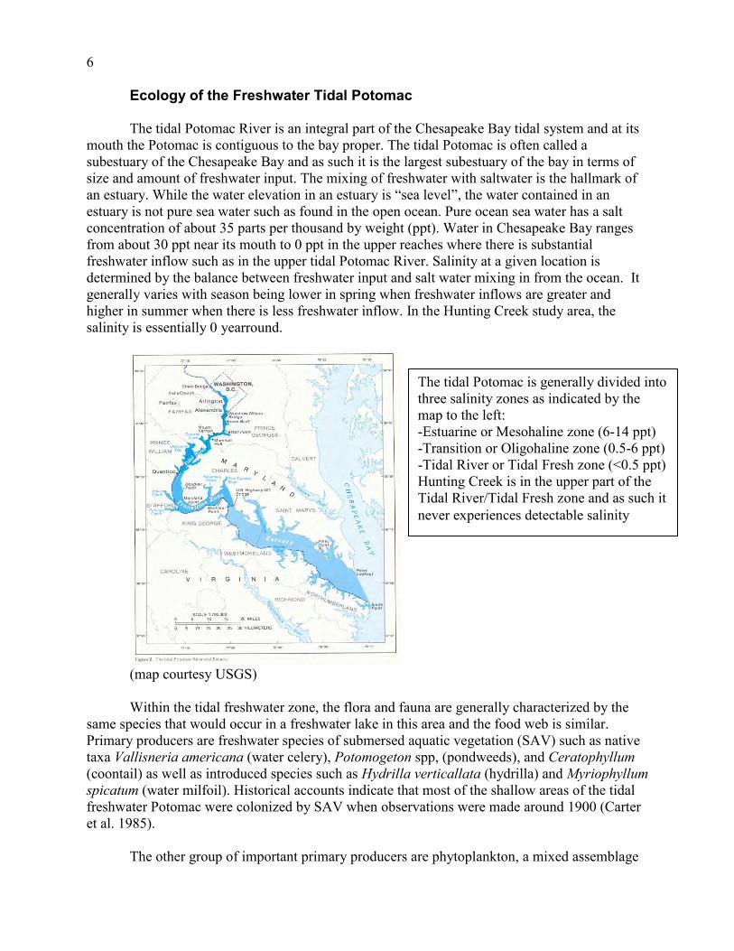
mouth the Potomac is contiguous to the bay proper. The tidal Potomac is often called a subestuary of the Chesapeake Bay and as such it is the largest subestuary of the bay in terms of size and amount of freshwater input. The mixing of freshwater with saltwater is the hallmark of an estuary. While the water elevation in an estuary is “sea level”, the water contained in an estuary is not pure sea water such as found in the open ocean. Pure ocean sea water has a salt concentration of about 35 parts per thousand by weight (ppt). Water in Chesapeake Bay ranges from about 30 ppt near its mouth to 0 ppt in the upper reaches where there is substantial freshwater inflow such as in the upper tidal Potomac River. Salinity at a given location is determined by the balance between freshwater input and salt water mixing in from the ocean. It generally varies with season being lower in spring when freshwater inflows are greater and higher in summer when there is less freshwater inflow. In the Hunting Creek study area, the salinity is essentially 0 yearround.

(map courtesy USGS) Within the tidal freshwater zone, the flora and fauna are generally characterized by the

same species that would occur in a freshwater lake in this area and the food web is similar. Primary producers are freshwater species of submersed aquatic vegetation (SAV) such as native taxa Vallisneria americana (water celery), Potomogeton spp, (pondweeds), and Ceratophyllum (coontail) as well as introduced species such as Hydrilla verticallata (hydrilla) and Myriophyllum spicatum (water milfoil). Historical accounts indicate that most of the shallow areas of the tidal freshwater Potomac were colonized by SAV when observations were made around 1900 (Carter et al. 1985).

The other group of important primary producers are phytoplankton, a mixed assemblage

The tidal Potomac is generally divided into three salinity zones as indicated by the map to the left: -Estuarine or Mesohaline zone (6-14 ppt) -Transition or Oligohaline zone (0.5-6 ppt) -Tidal River or Tidal Fresh zone (<0.5 ppt) Hunting Creek is in the upper part of the Tidal River/Tidal Fresh zone and as such it never experiences detectable salinity

7 of algae and cyanobacteria which may turn over rapidly on a seasonal basis. The dominant groups of phytoplankton in the tidal freshwater Potomac are diatoms (considered a good food source for aquatic consumers) and cyanobacteria (considered a less desirable food source for aquatic consumers). For the latter part of the 20th century, the high nutrient loadings into the river favored cyanobacteria over both diatoms and SAV resulting in large production of undesirable food for consumers. In the last decade or so, as nutrient reductions have become manifest, cyanobacteria have decreased and diatoms and SAV have increased.

The biomass contained in the cells of phytoplankton nourishes the growth of zooplankton

and benthic macroinvertebrates which provide an essential food supply for the juvenile and smaller fish. These in turn provide food for the larger fish like striped bass and largemouth bass. The species of zooplankton and benthos found in the tidal fresh zone are similar to those found in lakes in the area, but the fish fauna is augmented by species that migrate in and out from the open interface with the estuary.

Resident fish species include typical lake species such as sunfish (Lepomis spp.), bass

(Micropterus spp.), and crappie (Pomoxis spp.) as well as estuarine species such as white perch (Morone americana) and killifish (Fundulus spp.). Species which spend part of their year in the area include striped bass (Morone saxitilis) and river herrings and shad (Alosa spp.). Non-native fish species have also become established in the tidal freshwater Potomac such as northern snakehead (Channa argus) and blue catfish (Ictalurus furcatus).

Larval fishes are transitional stages in the development of juvenile fishes. They range in

development from newly hatched, embryonic fish to juvenile fish with morphological features similar to those of an adult. Many fishes such as clupeids (herring family), white perch, striped bass, and yellow perch disperse their eggs and sperm into the open water. The larvae of these species are carried with the current and termed “ichthyoplankton”. Other fish species such as sunfish and bass lay their eggs in “nests” on the bottom and their larvae are rare in the plankton.

After hatching from the egg, the larva draws nutrition from a yolk sack for a few days.

When the yolk sack diminishes to nothing, the fish begins a life of feeding on other organisms. This post yolk sack larva feeds on small planktonic organisms (mostly small zooplankton) for a period of several days. It continues to be a fragile, almost transparent larva and suffers high mortality to predatory zooplankton and juvenile and adult fishes of many species, including its own. When it has fed enough, it changes into an opaque juvenile, with greatly enhanced swimming ability. It can no longer be caught with a slow-moving plankton net, but is soon susceptible to capture with the seine or trawl net.

8

METHODS A. Profiles and Plankton: Sampling Day

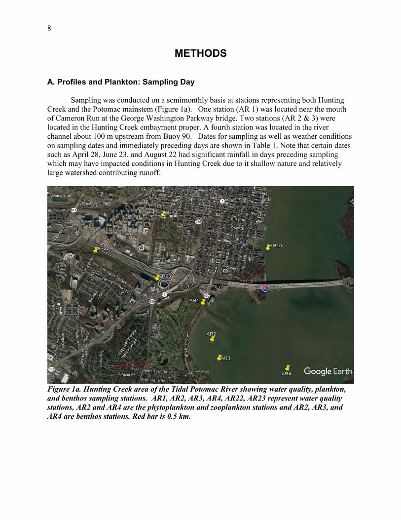
Sampling was conducted on a semimonthly basis at stations representing both Hunting

Creek and the Potomac mainstem (Figure 1a). One station (AR 1) was located near the mouth of Cameron Run at the George Washington Parkway bridge. Two stations (AR 2 & 3) were located in the Hunting Creek embayment proper. A fourth station was located in the river channel about 100 m upstream from Buoy 90. Dates for sampling as well as weather conditions on sampling dates and immediately preceding days are shown in Table 1. Note that certain dates such as April 28, June 23, and August 22 had significant rainfall in days preceding sampling which may have impacted conditions in Hunting Creek due to it shallow nature and relatively large watershed contributing runoff.

Figure 1a. Hunting Creek area of the Tidal Potomac River showing water quality, plankton, and benthos sampling stations. AR1, AR2, AR3, AR4, AR22, AR23 represent water quality stations, AR2 and AR4 are the phytoplankton and zooplankton stations and AR2, AR3, and AR4 are benthos stations. Red bar is 0.5 km.

9

Figure 1b. Cameron Run portion of the study area showing water quality stations.

Figure 1c. Hunting Creek area of the Tidal Potomac River showing fish monitoring stations.

PotomacRiver

4-Trawl3-Trawl

5-Seine

6-Seine

Hun ngCreek

Fykenet

Fykenet

10

Table 1

Hunting Creek Study: Sampling Dates and Weather Data for 2016 Type of Sampling Avg Daily Temp (oC) Precipitation (cm) Date WP B D T S F 1-Day 3-Day 1-Day 3-Day April 27 X 16.7 19.8 0.08 0.08 April 28 X X 11.1 17.4 1.47 1.55 May 10 X X 16.1 15.7 0.03 0.28 May 12 X X X 16.7 15.7 0 1.07 May 25 X 22.8 20.9 0 0.47 May 26 X X 24.4 22.8 0 T June 8 X X 20.0 23.3 0 T June 9 X X X 20.0 21.5 0 T June 22 X X X 25.6 26.7 0 2.51 June 23 X X (AR4) 24.4 25.9 1.35 3.86 July 6 X X X 30.0 26.7 0 1.47 July 7 X X 29.4 29.3 0 0.69 July 20 1 X X 26.7 27.6 0 2.29 July 25 X 32.8 32.0 0 T

August 5 X 26.1 25.7 T T August 8 X X 27.2 28.1 0 0.15 August 10 1 X X 30.0 27.0 0 T August 22 X 25.0 27.2 0 1.75 August 24 1 X X 25.0 24.8 0 0 September 6 X X 28.3 25.9 0 0 September 7 X 1 X X 28.9 27.4 0.05 0.05 September 20 X Type of Sampling: WP: Water quality (samples to AlexRenew Lab), profiles and plankton, B: benthos (station numbers indicated), D: dataflow (water quality mapping), T: fish collected by trawling, S: fish collected by seining. F: fish collected by fyke net. T under Precipitation equals “trace”. X indicates full station suite on that date. 1 on Trawl indicates only AR4.

11

Sampling was initiated about 10:00 am. Four types of measurements or samples were obtained at each station: (1) depth profiles of temperature, conductivity, dissolved oxygen, pH, and irradiance (photosynthetically active radiation, PAR) measured directly in the field; (2) water samples for GMU lab determination of chlorophyll a and phytoplankton species composition and abundance; (3) water samples for determination of N and P forms, BOD, COD, alkalinity, hardness, suspended solids, chloride, and pH by the Alexandria Renew Enterprises lab; (4) net sampling of zooplankton and ichthyoplankton.

Profiles of temperature, conductivity, and dissolved oxygen were conducted at each station using a YSI 6600 datasonde with temperature, conductivity, dissolved oxygen and pH probes. Measurements were taken at 0.3 m increments from surface to bottom at the embayment stations. In the river measurements were made with the sonde at depths of 0.3 m and 2.0 m increments to the bottom. Meters were checked for calibration before and after sampling. Profiles of irradiance (photosynthetically active radiation, PAR) were collected with a LI-COR underwater flat scalar PAR probe. PAR measurements were taken at 10 cm intervals to a depth of 1.0 m. Simultaneous measurements were made with a terrestrial probe in air during each profile to correct for changes in ambient light if needed. Secchi depth was also determined. The readings of at least two crew members were averaged due to variability in eye sensitivity among individuals. If the Secchi disk was still visible at the bottom or if its path was block by SAV while still visible, a proper reading could not be obtained.

A 1-liter depth-composited sample for GMU lab work was constructed from equal volumes of water collected at each of three depths (0.3 m below the surface, middepth, and 0.3 m off of the bottom) using a submersible bilge pump. A 100-mL aliquot of this sample was preserved immediately with acid Lugol’s iodine for later identification and enumeration of phytoplankton at stations AR2 and AR4. The remainder of the sample was placed in an insulated cooler with ice. A separate 1-liter surface sample was collected from 0.3 m using the submersible bilge pump and placed in the insulated cooler with ice for lab analysis of surface chlorophyll a.

At embayment and river mainstream sampling stations (AR2, AR3, and AR4), 2-liter

samples were collected monthly at each station from just below the surface (0.3 m) and near the bottom (0.3 m off bottom) at each station using the submersible pump. At tributary stations (AR1, AR 10, AR11, AR12, AR13, AR21, AR22, AR23, and AR30), 2-liter samples were collected by hand from just below the surface. This water was promptly delivered to the nearby Alexandria Renew Laboratory for determination of nitrogen, phosphorus, BOD, TSS, VSS, pH, total alkalinity, and chloride.

At stations AR2 and AR4, microzooplankton was collected by pumping 32 liters from each of three depths (0.3 m, middepth, and 0.3 m off the bottom) through a 44 μm mesh sieve. The sieve consisted of a 12-inch long cylinder of 6-inch diameter PVC pipe with a piece of 44 μm nitex net glued to one end. The 44 μm cloth was backed by a larger mesh cloth to protect it. The pumped water was passed through this sieve from each depth and then the collected microzooplankton was backflushed into the sample bottle. The resulting sample was treated with about 50 mL of club soda and then preserved with formalin containing a small amount of rose bengal to a concentration of 5-10%.

12

At stations AR2 and AR4, macrozooplankton was collected by towing a 202 µm net (0.3 m opening, 2 m long) for 1 minute at each of three depths (near surface, middepth, and near bottom). Ichthyoplankton (larval fish) was sampled by towing a 333 µm net (0.5 m opening, 2 m long) for 2 minutes at each of the same depths at Stations AR2 and AR4. In the embayment, the boat traveled from AR2 toward AR3 during the tow while in the river the net was towed in a linear fashion along the channel. Macrozooplankton tows were about 300 m and ichthyoplankton tows about 600 m. Actual distance depended on specific wind conditions and tidal current intensity and direction, but an attempt was made to maintain a constant slow forward speed (approximately 2 miles per hour) through the water during the tow. The net was not towed directly in the wake of the engine. A General Oceanics flowmeter, fitted into the mouth of each net, was used to establish the exact towing distance. During towing the three depths were attained by playing out rope equivalent to about 1.5-2 times the desired depth. Samples which had obviously scraped bottom were discarded and the tow was repeated. Flowmeter readings taken before and after towing allowed precise determination of the distance towed and when multiplied by the area of the opening produced the total volume of water filtered. Macrozooplankton were preserved immediately with rose bengal formalin with club soda pretreatment. Ichthyoplankton was preserved in 70% ethanol. Macrozooplankton was collected on each sampling trip; ichthyoplankton collections ended after July because larval fish were normally not found after this time. Benthic macroinvertebrate samples were collected monthly at stations AR2, AR3, and AR4. Three samples were collected at each station using a petite ponar grab. The bottom material was sieved through a 0.5 mm stainless steel sieve and resulting organisms were preserved in rose bengal formalin for lab analysis. Samples for water quality determination were maintained on ice and delivered to the Alexandria Renew Enterprises (AlexRenew) Laboratory by 2 pm on sampling day and returned to GMU by 3 pm. At GMU 10-15 mL aliquots of both depth-integrated and surface samples were filtered through 0.45 µm membrane filters (Gelman GN-6 and Millipore MF HAWP) at a vacuum of less than 10 lbs/in2 for chlorophyll a and pheopigment determination. During the final phases of filtration, 0.1 mL of MgCO3 suspension (1 g/100 mL water) was added to the filter to prevent premature acidification. Filters were stored in 20 mL plastic scintillation vials in the lab freezer for later analysis. Seston dry weight and seston organic weight were measured by filtering 200-400 mL of depth-integrated sample through a pretared glass fiber filter (Whatman 984AH). Sampling day activities were normally completed by 5:30 pm. B. Profiles and Plankton: Follow-up Analyses Chlorophyll a samples were extracted in a ground glass tissue grinder to which 4 mL of dimethyl sulfoxide (DMSO) was added. The filter disintegrated in the DMSO and was ground for about 1 minute by rotating the grinder under moderate hand pressure. The ground suspension was transferred back to its scintillation vial by rinsing with 90% acetone. Ground

13

samples were stored in the refrigerator overnight. Samples were removed from the refrigerator and centrifuged for 5 minutes to remove residual particulates. Chlorophyll a concentration in the extracts was determined fluorometrically using a Turner Designs Model 10 field fluorometer configured for chlorophyll analysis as specified by the manufacturer. The instrument was calibrated using standards obtained from Turner Designs. Fluorescence was determined before and after acidification with 2 drops of 10% HCl. Chlorophyll a was calculated from the following equation which corrects for pheophytin interference: Chlorophyll a (µg/L) = FsRs(Rb-Ra)/(Rs-1) where Fs=concentration per unit fluorescence for pure chlorophyll a Rs=fluorescence before acid/fluorescence after acid for pure chlorophyll a Rb=fluorescence of sample before acid Ra=fluorescence of sample after acid All chlorophyll analyses were completed within one month of sample collection. Phytoplankton species composition and abundance was determined using the inverted microscope-settling chamber technique (Lund et al. 1958). Ten milliters of well-mixed algal sample were added to a settling chamber and allowed to stand for several hours. The chamber was then placed on an inverted microscope and random fields were enumerated. At least two hundred cells were identified to species and enumerated on each slide. Counts were converted to number per mL by dividing number counted by the volume counted. Biovolume of individual cells of each species was determined by measuring dimensions microscopically and applying volume formulae for appropriate solid shapes. Microzooplankton and macrozooplankton samples were rinsed by sieving a well-mixed subsample of known volume and resuspending it in tap water. This allowed subsample volume to be adjusted to obtain an appropriate number of organisms for counting and for formalin preservative to be purged to avoid fume inhalation during counting. One mL subsamples were placed in a Sedgewick-Rafter counting cell and whole slides were analyzed until at least 200 animals had been identified and enumerated. A minimum of two slides was examined for each sample. References for identification were: Ward and Whipple (1959), Pennak (1978), and Rutner-Kolisko (1974). Zooplankton counts were converted to number per liter (microzooplankton) or per cubic meter (macrozooplankton) with the following formula: Zooplankton (#/L or #/m3) = NVs/(VcVf) where N = number of individuals counted Vs = volume of reconstituted sample, (mL) Vc = volume of reconstituted sample counted, (mL) Vf = volume of water sieved, (L or m3) Larval fish were picked from the ethanol-preserved ichthyoplankton samples with the

14

aid of a stereo dissecting microscope. Identification of ichthyoplankton was made to family and further to genus and species where possible. If the number of animals in the sample exceeded several hundred, then the sample was split with a plankton splitter and the resulting counts were multiplied by the subsampling factor. The works Hogue et al. (1976), Jones et al. (1978), Lippson and Moran (1974), and Mansueti and Hardy (1967) were used for identification. The number of ichthyoplankton in each sample was expressed as number per 10 m3 using the following formula: Ichthyoplankton (#/10m3) = 10N/V

where N = number ichthyoplankton in the sample V = volume of water filtered, (m3) C. Adult and Juvenile Fish Fishes were sampled by trawling at stations AR3 and AR4, and seining at stations AR5 and AR6 (Figure 1). For trawling, a try-net bottom trawl with a 15-foot horizontal opening, a ¾ inch square body mesh and a ¼ inch square cod end mesh was used. The otter boards were 12 inches by 24 inches. Towing speed was 2-3 miles per hour and tow length was 5 minutes. The trawls were towed upriver parallel to the channel at AR4, and following the curve away from the channel at AR3. The direction of tow should not be crucial. Dates of sampling and weather conditions are found in Table 1. Seining was performed with a bag seine that was 50 feet long, 3 feet high, and made of knotted nylon with a ¼ inch square mesh. The bag is located in the middle of the net and measures 3 ft3. The seining procedure was standardized as much as possible. The net was stretched out perpendicular to the shore with the shore end right at the water line. The net was then pulled parallel to the shore for a distance of 100 feet by a worker at each end moving at a slow walk. Actual distance was recorded if in any circumstance it was lower than 100 feet. At the end of the prescribed distance, the offshore end of the net was swung in an arc to the shore and the net pulled up on the beach to trap the fish. Dates for seine sampling were the same as those for trawl sampling (Table 1). Due to extensive submerged aquatic vegetation (SAV) cover in Hunting Creek, we adjusted our sampling regime in 2016. The trawl at AR3 has been impeded more frequently each year due to this vegetation, and two fyke nets were set in the area close to AR3 (Figure 1). The fyke net sampling stations are called ‘fyke near’ and ‘fyke far’ in reference to their distance from shore. These fyke nets were set within the SAV to sample the fish community that uses the SAV cover as habitat. Fyke nets were set for 4 hours to passively collect fish. The fyke nets have 5 hoops, a 1/4 inch mesh size, 16 feet wings and a 32 feet lead. Fish enter the net by actively swimming and/or due to tidal motion of the water. The lead increases catch by capturing the fish swimming parallel to the wings. Fyke nets were set each sampling date, and trawling in this location (AR3) became impossible by mid-July (Table 1). Utilizing the fyke nets when trawling is still possible allows for gear comparison. After the catch from each of these three gear types was hauled in, the fishes were measured for standard length and total length to the nearest mm. Standard length is the

15

distance from the front tip of the snout to the end of the vertebral column and base of the caudal fin. This is evident in a crease perpendicular to the axis of the body when the caudal fin is pulled to the side. Total length is the distance from the tip of the snout to the tip of the longer lobe of the caudal fin, measured by straightening the longer lobe toward the midline. If the identification of the fish was not certain in the field, a specimen was preserved in 70% ethanol and identified later in the lab. Fishes kept for chemical analysis were kept on ice wrapped in aluminum foil until frozen in the lab. All fishes retained for laboratory analysis or identification were first euthanized by submerging them in an ice sludge conforming to the AICUC protocol. Identification was based on characteristics in dichotomous keys found in several books and articles, including Jenkins and Burkhead (1983), Hildebrand and Schroeder (1928), Loos et al (1972), Dahlberg (1975), Scott and Crossman (1973), Bigelow and Schroeder (1953), Eddy and Underhill (1978), Page and Burr (1998), and Douglass (1999). D. Submersed Aquatic Vegetation Data on coverage and composition of submersed aquatic vegetation (SAV) are generally obtained from the SAV webpage of the Virginia Institute of Marine Science (http://www.vims.edu/bio/sav). Information on this web site is obtained from aerial photographs near the time of peak SAV abundance as well as ground surveys which are used to determine species composition. At the time of the draft report preparation, VIMS data was not available, but we did do some mapping of relative abundance of SAV species was obtained at regular site during the data mapping runs. E. Benthic Macroinvertebrates Benthic macroinvertebrates were sampled monthly using a petite ponar sampler at embayment stations AR2, AR3, and AR4. Triplicate samples were collected at each station monthly. Bottom samples were sieved on-site through a 0.5 mm stainless steel sieve and preserved with rose bengal formalin. In the laboratory benthic samples were rinsed with tap water through a 0.5 mm sieve to remove formalin preservative and resuspended in tap water. All organisms were picked, sorted, identified and enumerated. At the time of draft report preparation, the benthic data from embayment stations was not available. In 2016 for the first time, benthic invertebrates were also sampled at selected flowing tributary stations which possessed natural riffle-run areas. At each site one-minute kick samples were collected at one riffle and one run and composited in a single bottle. The sample was preserved with formalin to a concentration of 5%. In the lab the sample was sieved through a 0.5 mm mesh (same as the kick net) and thoroughly washed with tap water before picking and sorting. Following sorting animals were enumerated by taxon and held in ethanol-glycerin. Sampling sites for tributary macroinvertebrate sampling are shown in Figure 1d.

http://www.vims.edu/bio/sav

16

Figure 1d. Western portion of the study area showing benthic sampling stations on flowing tributaries of Cameron Run. CR1: Cameron Run: HR1, HR2: Holmes Run; BR: Backlick Run; IR: Indian Run; TR: Turkeycock Run. Red bar is 0.5 km. F. Water Quality Mapping (Dataflow) On two additional dates in 2016 (August 5 and September 7) in situ water quality mapping was conducted by slowly transiting through much of the Hunting Creek study area as water was pumped through a chamber containing a YSI 6600 sonde equipped with temperature, specific conductance, dissolved oxygen, pH, turbidity, and chlorophyll probes. Readings were recorded at 15 second intervals along with simultaneous GPS position readings. Every 2 minutes SAV relative abundance by species was recorded and every 4 minutes water samples were collected for extracted chlorophyll and TSS determination. Some areas of the Hunting Creek embayment could not be surveyed due to shallow water or heavy SAV growth. These surveys allowed a much better understanding of spatial patterns in water quality within the Hunting Creek area which facilitated interpretation of data from the fixed stations. This approach is in wide use in the Chesapeake Bay region by both Virginia and Maryland under the name “dataflow”. G. Data Analysis

Data for each parameter were entered into spreadsheets (Excel or SigmaPlot) for graphing of temporal and spatial patterns. SYSTAT was used for statistical calculations and to create illustrations of the water quality mapping cruises. JMP v8.0.1was used for fish graphs. Other data analysis approaches are explained in the text.

17

RESULTS

A. Climatic and Hydrologic Factors In 2016 air temperature was substantially above average from July through October (Table 2). July and August were the warmest months, with August and September being the most above normal. There were 52 days with maximum temperature above 32.2oC (90oF) during 2016 compared with 4 in 2004, 18 in 2005, 29 in 2006, 33 in 2007, 31 in 2008, 16 days in 2009, 62 in 2010, 42 in 2011, 42 in 2012, 27 in 2013, 20 in 2014, and 41 in 2015. Precipitation was well above normal during May, near normal from June through August, and below normal in October and November. The largest daily rainfall totals during the period of sampling were: 3.15 cm on May 2, 2.95 cm on August 15 and 2.24 cm on August 17. Table 2. Meteorological Data for 2016. National Airport. Monthly Summary. Air Temp Precipitation MONTH (oC) (cm) March 11.9 (8.1) 3.0 (9.1) April 13.8 (13.4) 5.2 (7.0) May 17.7 (18.7) 14.4 (9.7) June 24.6 (23.6) 9.4 (8.0) July 28.2 (26.2) 8.0 (9.3) August 28.2 (25.2) 7.1 (8.7) September 24.4 (21.4) 6.4 (9.6) October 17.3 (14.9) 2.3 (8.2) November 11.4 (9.3) 1.9 (7.7) December 5.4 (4.2) 6.6 (7.8) Note: 2014 monthly averages or totals are shown accompanied by long-term monthly averages (1971-2000). Source: Local Climatological Data. National Climatic Data Center, National Oceanic and Atmospheric Administration.

Table 3. Monthly mean discharge at USGS Stations representing freshwater flow into the study area. (+) 2016 month > 2x Long Term Avg. (-) 2015 month < ½ Long Term Avg.

Potomac River at Little Falls (cfs) Cameron Run at Wheeler Ave (cfs)

2016 Long Term Average 2016 Long Term Average

January 13487 13700 39.2 41 February 39524 (+) 16600 114.0 (+) 45 March 13844 23600 20.5 (-) 55 April 7258 (-) 20400 25.0 42 May 19954 15000 55.4 41 June 11016 9030 38.6 38 July 4674 4820 20.4 31 August 3925 4550 28.1 28 September 2177 (-) 5040 38.1 38 October 7504 5930 33.9 33

18

Potomac River at Little Falls (USGS 01646500)

Mar Apr May Jun Jul Aug Sep Oct Nov Dec Jan

Pot

omac

Riv

er D

isch

arge

(ft3 /s

ec)

103

104

105

Avg: 1988-20022016 Daily Flow

Figure 2. Mean Daily Discharge: Potomac River at Little Falls (USGS Data). Month tick is at

the beginning of the month.

Potomac River discharge during 2016 was below normal during March and April (Table 3, Figure 2). From May through July Potomac flows were consistently above the long-term mean. August experienced two significant flow events, but September was consistently slightly below the long term average. In Hunting Creek flows were generally below the long term average except for a few one-day spikes associated with storms. Water quality/plankton sampling dates that may have been particularly affected by immediately prior storm events include June 23 and to a less extent August 22 (Table 1).

.

Cameron Run at Alexandria VA (USGS 01653000)

Mar Apr May Jun Jul Aug Sep Oct Nov Dec Jan

Cam

eron

Run

Dis

char

ge (f

t3 /sec

)

1

10

100

1000

Avg: 1988-2013 2016: Daily flow

Figure 3. Mean Daily Discharge: Cameron Run at Alexandria (Wheeler Ave) (USGS Data).

In a tidal freshwater system like the Potomac River, river flow entering from upstream is important in maintaining freshwater conditions and also serves to bring in dissolved and particulate substances from the watershed. High freshwater flows may also flush planktonic organisms downstream and bring in suspended sediments that decrease water clarity. The volume of river flow per unit time is referred to as “river discharge” by hydrologists. Note the general long term seasonal pattern of higher discharges in winter and spring and lower discharges in summer and fall.

In the Hunting Creek region of the tidal Potomac, freshwater discharge is occurring from both the major Potomac River watershed upstream (measured at Little Falls) and from immediate tributaries, principally Cameron Run which empties directly into Hunting Creek. The gauge on Cameron Run at Wheeler Avenue is located just above the head of tide and covers most area which contributes runoff directly to the Hunting Creek embayment from the watershed. The contributing area to the Wheeler Ave gauge is 33.9 sq mi. (USGS)

19

B. Physico-chemical Parameters: Embayment and River Stations – 2016

Hunting Creek Study - 2016

Apr May Jun Jul Aug Sep Oct

Tem

pera

ture

(oC

)

0

5

10

15

20

25

30

35

Sta 1Sta 2 Sta 3Sta 4

Figure 4. Water Temperature (oC). GMU Field Data. Month tick is at first day of month.

In 2016, water temperature followed the typical seasonal pattern at all stations (Figure 4). Values were unusually high in late April, but consistently increased from May through late July. Maximum temperature was just above 30°C at all sites on July 25 and then declined through September. Mean daily air temperature showed similar patterns (Figure 5)

National Airport - 2014

Mar Apr May Jun Jul Aug Sep Oct

Ave

rage

Dai

ly A

ir Te

mpe

ratu

re (o C

)

0

10

20

30

40

Figure 5. Average Daily Air Temperature (oC) at Reagan National Airport.

Water temperature is an important factor affecting both water quality and aquatic life. In a well-mixed system like the tidal Potomac, water temperatures are generally fairly uniform with depth. In a shallow mixed system such as the tidal Potomac, water temperature often closely tracks daily changes in air temperature.

Mean daily air temperature (Figure 5) was a good predictor of water temperature (Figure 4).

20

Figure 6a. Water Quality Mapping. August 5, 2016. Temperature (°C).

Mapping of water temperature was conducted on two dates in 2015: August 5 and September 7. In August temperatures were noticably cooler in Hunting aCreek than in areas nearer the river mainstem whereas in August temperatures were higher in the shallow portions of Hunting Creek (Figure 6a&b). This can be explained by the fact that on August 5 a marked decline in temperature compared with previous days was observed and the opposite condition was found on the September date. The shallow water areas naturally responded more quickly to these changing weather conditions.

Figure 6b. Water Quality Mapping. September 7, 2016 Temperature (°C).

26272829

TEMPC

26272829

TEMPC

-77.06 -77.05 -77.04 -77.03 -77.02LONG

38.76

38.77

38.78

38.79

38.80LA

T

-77.06 -77.05 -77.04 -77.03 -77.02LONG

38.76

38.77

38.78

38.79

38.80LA

T

-77.06 -77.05 -77.04 -77.03 -77.02LONG

38.76

38.77

38.78

38.79

38.80LA

T

-77.06 -77.05 -77.04 -77.03 -77.02LONG

38.76

38.77

38.78

38.79

38.80LA

T

-77.06 -77.05 -77.04 -77.03 -77.02LONG

38.76

38.77

38.78

38.79

38.80

LAT

-77.06 -77.05 -77.04 -77.03 -77.02LONG

38.76

38.77

38.78

38.79

38.80

LAT

-77.06 -77.05 -77.04 -77.03 -77.02LONG

38.76

38.77

38.78

38.79

38.80

LAT

26.026.527.027.528.0

TEMPC

26.026.527.027.528.0

TEMPC

-77.06 -77.05 -77.04 -77.03 -77.02LONG

38.76

38.77

38.78

38.79

38.80

LAT

21



Spec

ific

Con

duct

ance

(uS/

cm)

0

100

200

300

400

500

600


Figure 7. Specific Conductance (µS/cm). GMU Field Data. Month tick is at first day of month.

Specific conductance exhibited a major decline from April to May at all sites (Figure 7). Then a general pattern of increase was observed at AR2, AR3, and AR4 for the remainder of the year. AR1 was much more variable: a strong decline in late June was attributable to major storm runoff, an increase in late July was not so easily explained. Chloride seasonal patterns (Figure 8) were similar to specific conductance at AR3 and AR4. The increase in chloride in late June at most sites is interesting in that this date followed a major runoff event which decreased specific conductance. It is not clear why chloride would increase under these conditions unless combined sewer inflows were involved.



Chl

orid

e (m

g/L)

0

20

40

60

80

100Sta 1Sta 2 Sta 3Sta 4

Specific conductance measures the capacity of the water to conduct electricity standardized to 25oC. This is a measure of the concentration of dissolved ions in the water. In freshwater, conductivity is relatively low. Ion concentration generally increases slowly during periods of low freshwater inflow and decreases during periods of high freshwater inflow. Sewage treatment facilities can be a source of elevated conductivity. In winter road salts can be a major source of conductivity in urban streams.

Figure 8. Chloride (mg/L). Alexandria Renew Lab Data. Month tick is at first day of

month.

Chloride ion (Cl-) is a principal contributor to conductance. Major sources of chloride in the study area are sewage treatment plant discharges, road salt, and brackish water from the downriver portion of the tidal Potomac. Chloride concentrations observed in the Hunting Creek area are very low relative to those observed in brackish, estuarine, and coastal areas of the Mid-Atlantic region. Chloride may increased slightly in late summer or fall when brackish water from down estuary may reach the area as freshwater discharge declines.

22

Figure 9a. Water Quality Mapping. August 5, 2016. Specific conductance (µS).

Mapping of specific conductance August 5 showed minor variations over most of the study are with lowest values along the Hunting Creek shoreline (Figure 9a&b). An area of elevated levels was observed in the river mainstem. On September 7 the highest values were observed in a small area of the embayment and lower values were found elsewhere, but again variations were minimal. Neither of these dates was affected by input of storm runoff. .

Figure 9b. Water Quality Mapping. September 7, 2017. Specific conductance (µS).

300350400450

SPCOND

300350400450

SPCOND

-77.06 -77.05 -77.04 -77.03 -77.02LONG

38.76

38.77

38.78

38.79

38.80LA

T

-77.06 -77.05 -77.04 -77.03 -77.02LONG

38.76

38.77

38.78

38.79

38.80LA

T

-77.06 -77.05 -77.04 -77.03 -77.02LONG

38.76

38.77

38.78

38.79

38.80LA

T

-77.06 -77.05 -77.04 -77.03 -77.02LONG

38.76

38.77

38.78

38.79

38.80LA

T

-77.06 -77.05 -77.04 -77.03 -77.02LONG

38.76

38.77

38.78

38.79

38.80

LAT

-77.06 -77.05 -77.04 -77.03 -77.02LONG

38.76

38.77

38.78

38.79

38.80

LAT

-77.06 -77.05 -77.04 -77.03 -77.02LONG

38.76

38.77

38.78

38.79

38.80

LAT

380390400410420

SPCOND

380390400410420

SPCOND

-77.06 -77.05 -77.04 -77.03 -77.02LONG

38.76

38.77

38.78

38.79

38.80

LAT

23



Dis

solv

ed O

xyge

n (m

g/L)

0

2

4

6

8

10

12

14


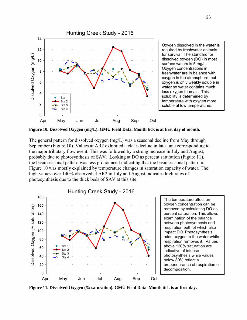
Figure 10. Dissolved Oxygen (mg/L). GMU Field Data. Month tick is at first day of month.

The general pattern for dissolved oxygen (mg/L) was a seasonal decline from May through September (Figure 10). Values at AR2 exhibited a clear decline in late June corresponding to the major tributary flow event. This was followed by a strong increase in July and August, probably due to photosynthesis of SAV. Looking at DO as percent saturation (Figure 11), the basic seasonal pattern was less pronounced indicating that the basic seasonal pattern in Figure 10 was mostly explained by temperature changes in saturation capacity of water. The high values over 140% observed at AR2 in July and August indicates high rates of photosynthesis due to the thick beds of SAV at this site.



Dis

solv

ed O

xyge

n (%

sat

urat

ion)

0

20

40

60

80

100

120

140

160

180


Figure 11. Dissolved Oxygen (% saturation). GMU Field Data. Month tick is at first day.

Oxygen dissolved in the water is required by freshwater animals for survival. The standard for dissolved oxygen (DO) in most surface waters is 5 mg/L. Oxygen concentrations in freshwater are in balance with oxygen in the atmosphere, but oxygen is only weakly soluble in water so water contains much less oxygen than air. This solubility is determined by temperature with oxygen more soluble at low temperatures.

The temperature effect on oxygen concentration can be removed by calculating DO as percent saturation. This allows examination of the balance between photosynthesis and respiration both of which also impact DO. Photosynthesis adds oxygen to the water while respiration removes it. Values above 120% saturation are indicative of intense photosynthesis while values below 80% reflect a preponderance of respiration or decomposition.

24

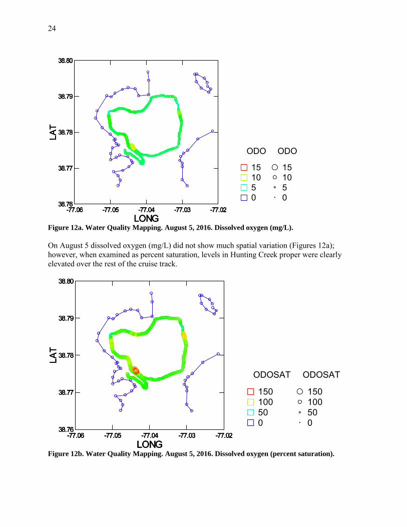
Figure 12a. Water Quality Mapping. August 5, 2016. Dissolved oxygen (mg/L).

On August 5 dissolved oxygen (mg/L) did not show much spatial variation (Figures 12a); however, when examined as percent saturation, levels in Hunting Creek proper were clearly elevated over the rest of the cruise track.

Figure 12b. Water Quality Mapping. August 5, 2016. Dissolved oxygen (percent saturation).

-77.06 -77.05 -77.04 -77.03 -77.02LONG

38.76

38.77

38.78

38.79

38.80LA

T

-77.06 -77.05 -77.04 -77.03 -77.02LONG

38.76

38.77

38.78

38.79

38.80LA

T

-77.06 -77.05 -77.04 -77.03 -77.02LONG

38.76

38.77

38.78

38.79

38.80LA

T

051015

ODO

051015

ODO

-77.06 -77.05 -77.04 -77.03 -77.02LONG

38.76

38.77

38.78

38.79

38.80LA

T

-77.06 -77.05 -77.04 -77.03 -77.02LONG

38.76

38.77

38.78

38.79

38.80

LAT

-77.06 -77.05 -77.04 -77.03 -77.02LONG

38.76

38.77

38.78

38.79

38.80

LAT

-77.06 -77.05 -77.04 -77.03 -77.02LONG

38.76

38.77

38.78

38.79

38.80

LAT

050100150

ODOSAT

050100150

ODOSAT

-77.06 -77.05 -77.04 -77.03 -77.02LONG

38.76

38.77

38.78

38.79

38.80

LAT

25

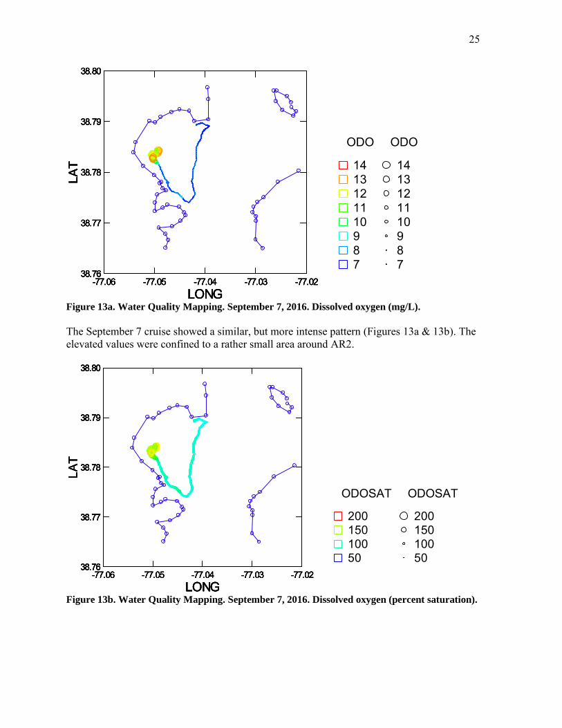
Figure 13a. Water Quality Mapping. September 7, 2016. Dissolved oxygen (mg/L).

The September 7 cruise showed a similar, but more intense pattern (Figures 13a & 13b). The elevated values were confined to a rather small area around AR2.

Figure 13b. Water Quality Mapping. September 7, 2016. Dissolved oxygen (percent saturation).

-77.06 -77.05 -77.04 -77.03 -77.02LONG

38.76

38.77

38.78

38.79

38.80LA

T

-77.06 -77.05 -77.04 -77.03 -77.02LONG

38.76

38.77

38.78

38.79

38.80LA

T

-77.06 -77.05 -77.04 -77.03 -77.02LONG

38.76

38.77

38.78

38.79

38.80LA

T

7891011121314

ODO

7891011121314

ODO

-77.06 -77.05 -77.04 -77.03 -77.02LONG

38.76

38.77

38.78

38.79

38.80LA

T

-77.06 -77.05 -77.04 -77.03 -77.02LONG

38.76

38.77

38.78

38.79

38.80

LAT

-77.06 -77.05 -77.04 -77.03 -77.02LONG

38.76

38.77

38.78

38.79

38.80

LAT

-77.06 -77.05 -77.04 -77.03 -77.02LONG

38.76

38.77

38.78

38.79

38.80

LAT

50100150200

ODOSAT

50100150200

ODOSAT

-77.06 -77.05 -77.04 -77.03 -77.02LONG

38.76

38.77

38.78

38.79

38.80

LAT

26



Fiel

d pH

6.0

6.5

7.0

7.5

8.0

8.5

9.0

9.5Sta 1Sta 2 Sta 3Sta 4

Figure 14. pH. GMU Field Data. Month tick is at first day of month.

Field pH and lab pH showed consistent seasonal and spatial patterns in 2016 (Figure 14, 15). The river mainstem site (AR 4) was fairly constant through time, generally in the 7.5-8.0 range, except for a clear increase in late June. The late June increased was observed at AR3, but not at AR1 or AR2. In July and August, pH increased markedly at AR2 and somewhat at AR3 in both field and lab measurements. These increases can be ascribed to active photosynthesis by SAV.



Lab

pH

6.0

6.5

7.0

7.5

8.0

8.5

9.0


Figure 15. pH. AlexRenew Lab Data. Month tick is at first day of month.

pH is a measure of the concentration of hydrogen ions (H+) in the water. Neutral pH in water is 7. Values between 6 and 8 are often called circumneutral, values below 6 are acidic and values above 8 are termed alkaline. Like DO, pH is affected by photosynthesis and respiration. In the tidal Potomac, pH above 8 indicates active photosynthesis and values above 9 indicate intense photosynthesis. A decrease in pH following a rainfall event may be due to acids in the rain or in the watershed.

pH may be measured in the field or in the lab. Field pH is more reflective of in situ conditions while lab pH is done under more stable and controlled laboratory conditions and is less subject to error. Newer technologies such as the Hydrolab and YSI sondes used in GMU field data collection are more reliable than previous field pH meters and should give results that are most representative of values actually observed in the river.

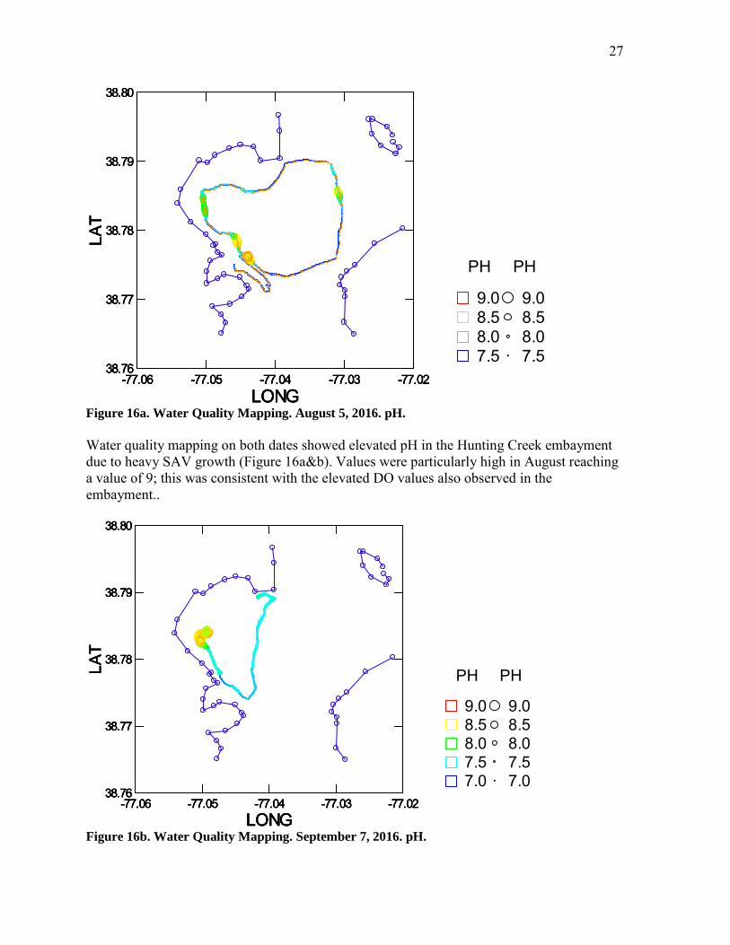
27

Figure 16a. Water Quality Mapping. August 5, 2016. pH.

Water quality mapping on both dates showed elevated pH in the Hunting Creek embayment due to heavy SAV growth (Figure 16a&b). Values were particularly high in August reaching a value of 9; this was consistent with the elevated DO values also observed in the embayment..

Figure 16b. Water Quality Mapping. September 7, 2016. pH.

-77.06 -77.05 -77.04 -77.03 -77.02LONG

38.76

38.77

38.78

38.79

38.80LA

T

-77.06 -77.05 -77.04 -77.03 -77.02LONG

38.76

38.77

38.78

38.79

38.80LA

T

-77.06 -77.05 -77.04 -77.03 -77.02LONG

38.76

38.77

38.78

38.79

38.80LA

T

7.58.08.59.0

PH

7.58.08.59.0

PH

-77.06 -77.05 -77.04 -77.03 -77.02LONG

38.76

38.77

38.78

38.79

38.80LA

T

-77.06 -77.05 -77.04 -77.03 -77.02LONG

38.76

38.77

38.78

38.79

38.80

LAT

-77.06 -77.05 -77.04 -77.03 -77.02LONG

38.76

38.77

38.78

38.79

38.80

LAT

-77.06 -77.05 -77.04 -77.03 -77.02LONG

38.76

38.77

38.78

38.79

38.80

LAT

7.07.58.08.59.0

PH

7.07.58.08.59.0

PH

-77.06 -77.05 -77.04 -77.03 -77.02LONG

38.76

38.77

38.78

38.79

38.80

LAT

28



Tota

la A

lkal

inity

(mg

CaC

O3/L

)

0

20

40

60

80

100

120

140


Figure 17. Total Alkalinity (mg/L as CaCO3). AlexRenew Lab data. Month tick is at first day.

Total alkalinity was generally in the range 60-100 mg/L as CaCO3 (Figure 17). Higher values were observed at AR2, AR3, and AR4 in April. A much lower value was observed in late June in the aftermath of runoff from the large rainfall event. It appears that the dry spring allowed alkalinity to build up and the runoff flushed some of it in June. Water clarity as reflected by Secchi disk transparency varied markedly over the year (Figure 18). Values at AR2 were low in April and early May, but increased in late May. Accurate values were missing from AR2 during most of the year as the Secchi disk was visible to the bottom of the bay or to the top of the SAV which was about 1 m. Values were more consistently obtained at AR3 which is also in the SAV beds indicating high levels of transparency. At AR4 in the channel, transparency reached a low value in early June and increased slowly the rest of the year.



Secc

hi D

isk

Dep

th (m

)

0.0

0.2

0.4

0.6

0.8

1.0

1.2

1.4


Figure 18. Secchi Disk Depth (m). GMU Field Data. Month tick is at first day of month.

Secchi Depth is a measure of the transparency of the water. The Secchi disk is a flat circle of thick sheet metal or plywood about 6 inches in diameter which is painted into alternate black and white quadrants. It is lowered on a calibrated rope or rod to a depth at which the disk disappears. This depth is termed the Secchi Depth. This is a quick method for determin-ing how far light is penetrating into the water column. Light is necessary for photosynthesis and thereby for growth of aquatic plants and algae.

Total alkalinity measures the amount of bicarbonate and carbonate dissolved in the water. In freshwater this corresponds to the ability of the water to absorb hydrogen ions (acid) and still maintain a near neutral pH. Alkalinity in the tidal freshwater Potomac generally falls into the moderate range allowing adequate buffering without carbonate precipitation.

29



Ligh

t Atte

nuat

ion

Coe

ffici

ent (

m-1

)

-5

-4

-3

-2

-1

0


Figure 19. Light Attenuation Coefficient (m-1). GMU Field Data. Month tick is at first day of

month.

Light attenuation coefficient data generally fell in the range -1.0 to -3.0 m-1 (Fiigure 19). Values were generally low in late April and increased strongly through late May. Turbidity showed a seasonal decline at AR1, AR2, and AR3 (Figure 20). At AR4 values generally trended upward from May through September.



YSI T

urbi

dity

0

10

20

30

40

50

60

70


Figure 20. Turbidity (NTU). GMU Lab Data. Month tick is at first day of month.

Light Attenuation is another approach to measuring light penetration. This is determined by measuring light levels at a series of depths starting near the surface. The resulting relationship between depth and light is fit to a semi-logarithmic curve and the resulting slope is called the light attenuation coefficient. This relationship is called Beer’s Law. It is analogous to absorbance on a spectrophotometer. The greater the light attenuation, the faster light is absorbed with depth. More negative values indicate greater attenuation. Greater attenuation is due to particulate and dissolved material which absorbs and deflects light.

Turbidity is yet a third way of measuring light penetration. Turbidity is a measure of the amount of light scattering by the water column. Light scattering is a function of the concentration and size of particles in the water. Small particles scatter more light than large ones (per unit mass) and more particles result in more light scattering than fewer particles.

30

Figure 21a. Water Quality Mapping. August 5, 2016. Turbidity YSI.

On the August mapping turbidity was highest near the river channel and lower in the SAV beds (Figure 21a). Within Hunting Creek values were generally in the 0-10 NTU range. In August turbidity was generally low in the area surveyed with one hot spot near the river channel (Figure 21b).

Figure 21b. Water Quality Mapping. September 7, 2016. Turbidity YSI.

-77.06 -77.05 -77.04 -77.03 -77.02LONG

38.76

38.77

38.78

38.79

38.80LA

T

-77.06 -77.05 -77.04 -77.03 -77.02LONG

38.76

38.77

38.78

38.79

38.80LA

T

-77.06 -77.05 -77.04 -77.03 -77.02LONG

38.76

38.77

38.78

38.79

38.80LA

T

-1001020

TURBID_

-1001020

TURBID_

-77.06 -77.05 -77.04 -77.03 -77.02LONG

38.76

38.77

38.78

38.79

38.80LA

T

-77.06 -77.05 -77.04 -77.03 -77.02LONG

38.76

38.77

38.78

38.79

38.80

LAT

-77.06 -77.05 -77.04 -77.03 -77.02LONG

38.76

38.77

38.78

38.79

38.80

LAT

-77.06 -77.05 -77.04 -77.03 -77.02LONG

38.76

38.77

38.78

38.79

38.80

LAT

010203040

TURBID_

010203040

TURBID_

-77.06 -77.05 -77.04 -77.03 -77.02LONG

38.76

38.77

38.78

38.79

38.80

LAT

31



Amm

onia

Nitr

ogen

(mg/

L)

0.0

0.1

0.2

0.3

0.4

0.5


Figure 22. Ammonia Nitrogen (mg/L). AlexRenew Lab Data. Month tick is at first day of

month.

Ammonia nitrogen was consistently low (<0.2 mg/L) for the entire study period (Figure 22). A clear seasonal pattern was seen at AR1, AR2, and AR3 with a general decline. At AR4 ammonia values dipped somewhat during the summer and rose again in September. Nitrate nitrogen levels showed a general seasonal decline at all sites (Figure 23). An unusually high value was observed at AR1 in late May. Nitrate levels reached very low values at AR2 in late July and August.



Nitr

ate

Nitr

ogen

(mg/

L)

0.0

0.5

1.0

1.5

2.0

2.5


Figure 23. Nitrate Nitrogen (mg/L). AlexRenew Lab Data. Month tick is at first day of month.

Ammonia nitrogen measures the amount of ammonium ion (NH4+) and ammonia gas (NH3) dissolved in the water. Ammonia nitrogen is readily available to algae and aquatic plants and acts to stimulate their growth. While phosphorus is normally the most limiting nutrient in freshwater, nitrogen is a close second. Ammonia nitrogen is rapidly oxidized to nitrate nitrogen when oxygen is present in the water so high ammonia levels suggest proximity to a source.

Nitrate Nitrogen refers to the amount of N that is in the form of nitrate ion (NO3-). Nitrate ion is the most common form of nitrogen in most well oxidized freshwater systems. Nitrate concentrations are increased by input of wastewater, nonpoint sources, and oxidation of ammonia in the water. Nitrate concentrations decrease when algae and plants are actively growing and removing nitrogen as part of their growth.

32



Nitr

ite N

itrog

en (m

g/L)

0.00

0.02

0.04

0.06


Figure 24. Nitrite Nitrogen (mg/L). AlexRenew Lab Data. Month tick is at first day of month.

Nitrite nitrogen was generally low (<0.03 mg/L) throughout the year (Figure 24). Organic nitrogen values were generally in the range of 0.2-0.6 mg/L with little clear seasonal or spatial pattern (Figure 25).



Org

anic

Nitr

ogen

(mg/

L)

0.0

0.2

0.4

0.6

0.8

1.0

1.2


Figure 25. Organic Nitrogen (mg/L). AlexRenew Lab Data. Month tick is at first day of month.

Nitrite nitrogen consists of nitrogen in the form of nitrite ion (NO2-). Nitrite is an intermediate in the oxidation of ammonia to nitrate, a process called nitrification. Nitrite is usually in very low concentrations unless there is active nitrification.

Organic nitrogen measures the nitrogen in dissolved and particulate organic compounds in the water. Organic nitrogen comprises algal and bacterial cells, detritus (particles of decaying plant, microbial, and animal matter), amino acids, urea, and small proteins. When broken down in the environment, organic nitrogen results in ammonia nitrogen. Organic nitrogen is determined as the difference between total Kjeldahl nitrogen and ammonia nitrogen.

33



Tota

l Pho

spho

rus

(mg/

L)

0.00

0.05

0.10

0.15

0.20


Figure 26. Total Phosphorus (mg/L). AlexRenew Lab Data. Month tick is at first day of month.

Total phosphorus showed little consistent seasonal pattern (Figure 26). In general total P was highest at AR4 and lowest at AR2. Ortho-phosphorus was generally quite low, but varied a lot from date to date and showed little consistent spatial pattern (Figure 27).



Orth

o-Ph

osph

orus

(mg/

L)

0.00

0.02

0.04

0.06

0.08


Figure 27. Soluble Reactive Phosphorus (mg/L). AlexRenew Lab Data. Month tick is at first day

of month.

Phosphorus (P) is often the limiting nutrient in freshwater ecosystems. As such the concentration of P can set the upper limit for algal growth. Total phosphorus is the best measure of P availability in freshwater since much of the P is tied up in biological tissue such as algal cells. Total P includes phosphate ion (PO4-

3) as well as phosphate inside cells and phosphate bound to inorganic particles such as clays.

Soluble reactive phosphorus (SRP) is a measure of phosphate ion (PO4-3). Phosphate ion is the form in which P is most available to primary producers such as algae and aquatic plants in freshwater. However, SRP is often inversely related to the activity of primary producers because they tend to take it up so rapidly. So, higher levels of SRP indicate either a local source of SRP to the waterbody or limitation by a factor other than P.

34



N to

P ra

tio b

y w

eigh

t

0

10

20

30

40

50


Figure 28. N/P Ratio (by mass). AlexRenew Lab Data. Month tick is at first day of month.

N/P ratio consistently pointed to P limitation being greater than 7.2 in almost all samples (Figure 28). A general seasonal decline was observed at all stations through early September. Biochemical oxygen demand (BOD) was often 1 or 2 mg/L at all stations (Figure 29).



BOD

(mg/

L)

0

1

2

3

4

5


Figure 29. Biochemical Oxygen Demand (mg/L). AlexRenew Lab Data. Month tick is at first

day of month.

N:P ratio is determined by summing all of the components of N (ammonia, nitrate, nitrite, and organic nitrogen) and dividing by total P. This ratio gives an indication of whether N or P is more likely to be limiting primary production in a given freshwater system. Generally, values above 7.2 are considered indicative of P limitation while values below 7.2 suggest N limitation. N limitation could lead to dominance by cyanobacteria who can fix their own N from the atmosphere.

Biochemical oxygen demand (BOD) measures the amount of decomposable organic matter in the water as a function of how much oxygen it consumes as it breaks down over a given number of days. Most commonly the number of days used is 5. BOD is a good indicator of the potential for oxygen depletion in water. BOD is composed both dissolved organic compounds in the water as well as microbes such as bacteria and algae which will respire and consume oxygen during the period of measurement.

35



Tota

l Sus

pend

ed S

olid

s (m

g/L)

0

10

20

30

40

50

60

70

80

90

100

110


Figure 30. Total Suspended Solids (mg/L). AlexRenew Lab Data. Month tick is at first day of

month.

Total suspended solids was generally in the range 0-20 mg/L (Figure 30). Values were generally highest at AR4 and lowest at AR2. VSS values were generally much lower (Figure 31). Both TSS and VSS were highly elevated in late June corresponding to the major runoff event.



Vola

tile

Susp

ende

d So

lids

(mg/

L)

0

20

40

60

80


Figure 31. Volatile Suspended Solids (mg/L). AlexRenew Lab Data. Month tick is at first day of

month.

Total suspended solids (TSS) is measured by filtering a known amount of water through a fine filter which retains all or virtually all particles in the water. This filter is then dried and the weight of particles on the filter determined by difference. TSS consists of both organic and inorganic particles. During periods of low river and tributary inflow, organic particles such as algae may dominate. During storm flow periods or heavy winds causing resuspension, inorganic particles may dominate.

Volatile suspended solids (VSS) is determined by taking the filters used for TSS and then ashing them to combust (volatilize) the organic matter. The organic component is then determined by difference. VSS is a measure of organic solids in a water sample. These organic solids could be bacteria, algae, or detritus. Origins include sewage effluent, algae growth in the water column, or detritus produced within the waterbody or from tributaries. In summer in Gunston Cove a chief source is algal (phytoplankton) growth.

36

C. Physico-chemical Parameters: Tributary Stations – 2016



Tem

pera

ture

(oC

)

0

5

10

15

20

25

30

35

Sta 11aSta 11b Sta 12Sta 13


Water quality data for the tributary stations is arranged in 2 groups: Stations 11, 12, and 13 represent stations accessed from the north side of Cameron Run and upper Hunting Creek. Stations AR21, AR22, and AR23 are accessed from the south side. AR 30 located at the farthest upstream reaches of Cameron Run. Temperatures at almost all stations closely followed air temperatures. The most obvious exception was AR13 which exhibited lower temperatures during most of the year. The water at AR13 is just emerging from underground storm sewers and is buffered from the higher air temperatures.



Tem

pera

ture

(oC

)

0

5

10

15

20

25

30

35

Sta 21Sta 22Sta 23Sta 30


37



Spec

ific

Con

duct

ance

(uS/

cm)

0

100

200

300

400

500

600

700


Figure 34. Specific Conductance (uS/cm). GMU Field Data. Month tick is at first day of month.

Specific conductance exhibited an overall gradual downward trend over time at all of the tributary stations (Figures 34 and 35). The most obvious deviation from this trend was the strong drop in specific conductance at all stations in late June. This corresponded with the aftermath of the largest precipitation event of the year and was probably the result of dilution with rainwater which is generally low in ions. The most precipitous declines were at AR13 and AR22. Another decline was observed at all stations in late August. This also appears due to a runoff even as 1.35 cm of rain had fallen in the 2 days prior to sampling. No other dates had experience substantial antecedent precipitation. The strong decline at AR21 was hard to explain.



Spec

ific

Con

duct

ance

(uS/

cm)

0

100

200

300

400

500

600

700


Figure 35. Specific Conductance (uS/cm). GMU Field Data. Month tick is at first day of month.

38



Dis

solv

ed O

xyge

n (m

g/L)

0

2

4

6

8

10

12

14

Sta 11aSta 11bSta 12Sta 13

Figure 36. Dissolved Oxygen (mg/L) GMU Field Data. Month tick is at first day of month.

Dissolved oxygen (mg/L) in the tributaries was generally in a range supportive of aquatic life (Figures 36 and 37). Several of the stations exhibited a gradual seasonal pattern that was probably reflective of changes in DO saturation with temperature. AR11a showed the most variability especially in late August and September. In the lower graph AR22 and AR23 were depressed in late June during the runoff event.



Dis

solv

ed O

xyge

n (m

g/L)

0

2

4

6

8

10

12


Figure 37. Dissolved Oxygen (mg/L) GMU Field Data. Month tick is at first day of month.

39



Dis

solv

ed O

xyge

n (%

sat

urat

ion)

0

20

40

60

80

100

120

140

160

180Sta 11aSta 11b Sta 12Sta 13

Figure 38. Dissolved Oxygen (% saturation) GMU Field Data. Month tick is at first day of

month. Dissolved oxygen as percent saturation is shown in Figures 38 and 39. Most of the seasonal pattern has disappeared. Several of the stations (AR12, AR13, AR21, AR30) remained near 100% saturation for the entire year. Several showed more variability. AR11b was consistently below saturation, but never dropped too much. AR11a was again the most variable showing significant depletion and supersaturation depending on the date. AR22 and AR23 were consistently slightly below saturation and did show a response to the late June flow event.



Dis

solv

ed O

xyge

n (%

sat

urat

ion)

0

20

40

60

80

100

120

140


Figure 39. Dissolved Oxygen (% saturation) GMU Field Data. Month tick is at first day of

month.

40



Fiel

d pH

6.0

6.5

7.0

7.5

8.0

8.5

9.0

9.5Sta 11aSta 11b Sta 12Sta 13

Figure 38. Field pH. GMU Field Data. Month tick is at first day of month. Field pH was consistently in the 6.5 to 8.0 range at tributary stations (Figures 38 and 39). AR12 exhibited one value above 8.0 in early July. These values are clearly in the range supportive of aquatic life. Somewhat surprisingly, there was no obvious response to the late June flow event.



Fiel

d pH

6.0

6.5

7.0

7.5

8.0

8.5

9.0

9.5Sta 21Sta 22Sta 23Sta 30

Figure 39. Field pH. GMU Field Data. Month tick is at first day of month.

41



YSI T

urbi

dity

0

20

40

60

80

100

120

140

160

180


Figure 40. YSI Turbidity. GMU Field Data. Month tick is at first day of month. Turbidity values were generally fairly low (<20 units) at all tributary stations (Figures 40 and 41). However, there was a very large response to the late June flow event at most stations. Particularly large spikes were observed at AR11a, AR11b, and AR30. Smaller, but still very obvious, increases were found at AR21, AR22, and AR23. A slight uptick was seen at AR13. The reason for the early August spike at AR13 and AR11b is not so clear given that there was no immediately prior rainfall and weather conditions were listed as clear in the databook.



YSI T

urbi

dity

0

20

40

60

80

100

120

140

160

180


Figure 41. YSI Turbidity. GMU Field Data. Month tick is at first day of month.

42



YSI C

hl a

(ug/

L)

0

20

40

60


Figure 42. YSI Chlorophyll a. GMU Field Data. Month tick is at first day of month.

YSI chlorophyll a was generally quite low (<5 ug/L) at most of the stations (Figures 42 and 43). Exceptions included AR11a, AR11b, and AR21. AR11a readings were taken in Lake Cook and these elevated values probably reflect growths of phytoplankton within the lake water column. AR11b was in the outlet and did had a similar pattern except in late May. The other station with high YSI chlorophyll readings was AR21 on certain dates. Since this station was just downstream from Lake Cook on Cameron Run, it may also be impacted by phytoplankton in its outflow.



YSI C

hl a

(ug/

L)

0

20

40

60

80Sta 21Sta 22Sta 23Sta 30

Figure 43. YSI Chlorophyll a. GMU Field Data. Month tick is at first day of month.

43



Lab

pH

6.0

6.5

7.0

7.5

8.0

8.5

9.0


Figure 44. Lab pH. AlexRenew Lab Data. Month tick is at first day of month.

Lab pH readings (Figures 44 and 45) were very similar to the field pH readings reviewed earlier. There was little difference among the stations or over time most readings being in the 6.7 to 7.7 range.



Lab

pH

6.0

6.5

7.0

7.5

8.0

8.5

9.0


Figure 45. Lab pH. AlexRenew Lab Data. Month tick is at first day of month.

44



Tota

la A

lkal

inity

(mg

CaC

O3/L

)

0

20

40

60

80

100

120

140


Figure 46. Total Alkalinity (mg/L as CaCO3) AlexRenew Lab Data. Month tick is at first day of

month. Total alkalinity was generally in the 45-65 mg/L range (Figures 46 and 47). At some of the stations there was a muted seasonal pattern of higher values in spring, lower values in mid summer, and increasing values in the fall. Slightly higher values were observed in early August at AR11a, in early September at AR22, and in July and early August at AR23. The higher values at AR23 are similar to the levels observed at AR1. These two stations are tidally connected and the Alex Renew effluent comes in near AR23 so this may be an explanation: high tides and/or possible effluent effects. A detectable decline was observed at several stations in the wake of the late June flow event.



Tota

la A

lkal

inity

(mg

CaC

O3/L

)

0

20

40

60

80

100

120

140


Figure 47. Total Alkalinity (mg/L as CaCO3) AlexRenew Lab Data. Month tick is at first day of

month.

45



Tota

l Pho

spho

rus

(mg/

L)

0.00

0.05

0.10

0.15

0.20

0.25


Figure 48. Total Phosphorus (mg/L) AlexRenew Lab Data. Month tick is at first day of month. Total phosphorus levels exhibited clear patterns at some stations (Figures 48 and 49). Most stations exhibited peaks in early May and late June with other values generally below 0.10 mg/L. The late June peak, clearly observed at AR12, AR21, AR22, AR23, and AR30, was attributable to the high flow event which was still ongoing at sample collection time. The lesser early May peak correlated with 0.28 cm of rainfall in the two days leading up to sampling. May generally was a very wet month. The erratic behavior at AR11a is related to events, probably algal blooms, in Lake Cook. AR13 is Hoofs Run which contains a mix of urban runoff and combined sewer overflows which could easily impact total P.



Tota

l Pho

spho

rus

(mg/

L)

0.00

0.05

0.10

0.15

0.20

0.25


Figure 49. Total Phosphorus (mg/L) AlexRenew Lab Data. Month tick is at first day of month.

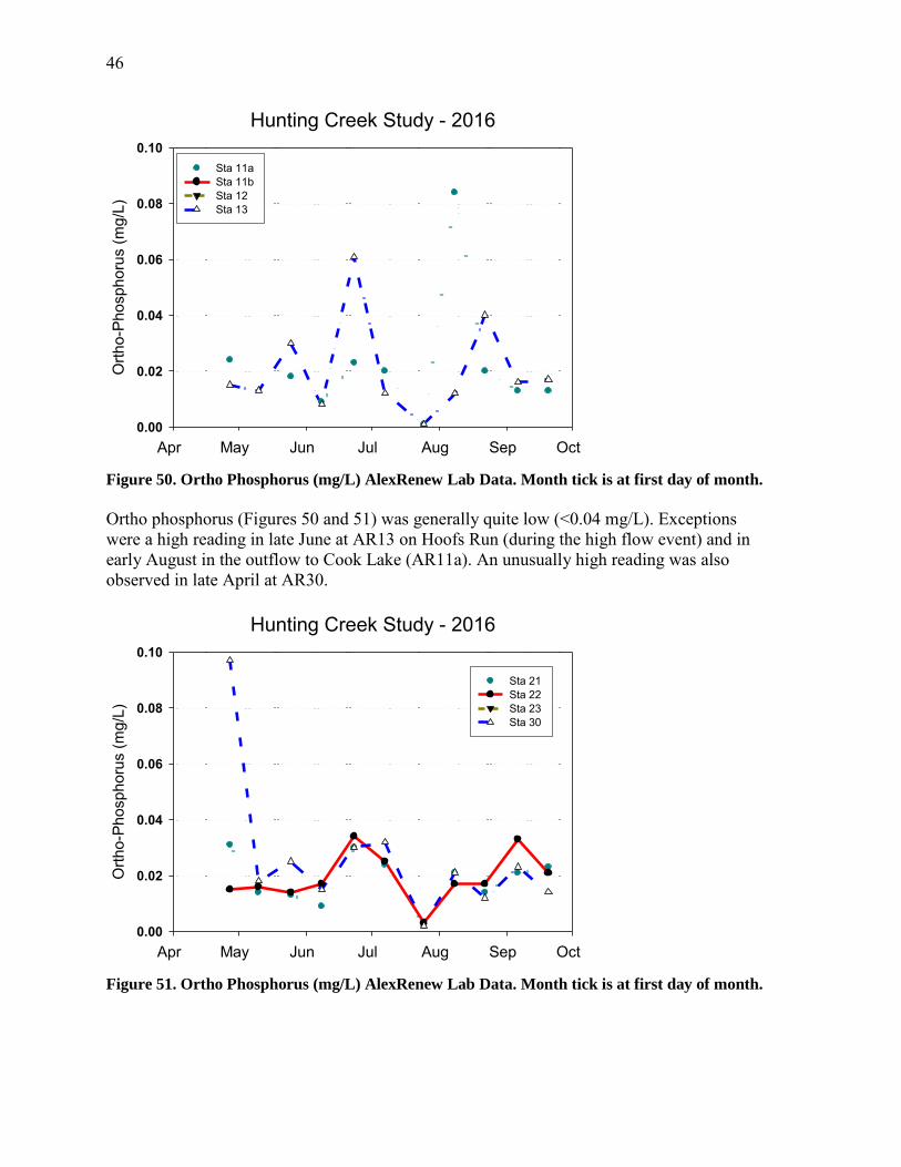
46



Orth

o-Ph

osph

orus

(mg/

L)

0.00

0.02

0.04

0.06

0.08


Figure 50. Ortho Phosphorus (mg/L) AlexRenew Lab Data. Month tick is at first day of month. Ortho phosphorus (Figures 50 and 51) was generally quite low (<0.04 mg/L). Exceptions were a high reading in late June at AR13 on Hoofs Run (during the high flow event) and in early August in the outflow to Cook Lake (AR11a). An unusually high reading was also observed in late April at AR30.



Orth

o-Ph

osph

orus

(mg/

L)

0.00

0.02

0.04

0.06

0.08

0.10


Figure 51. Ortho Phosphorus (mg/L) AlexRenew Lab Data. Month tick is at first day of month.

47



Org

anic

Nitr

ogen

(mg/

L)

0.0

0.2

0.4

0.6

0.8

1.0

1.2


Figure 52. Organic Nitrogen (mg/L) AlexRenew Lab Data. Month tick is at first day of month. Tributary levels of organic nitrogen are depicted in Figures 52 and 53. At several stations (AR12, AR21, AR22, and AR30) the most obvious pattern was a peak in late June during the flow event. Other stations displayed different patterns. AR11a showed a strong seasonal increase to well over 1.5 mg/L, reflecting events in Lake Cook. AR13 on Hoofs Run demonstrated a peak in early June. AR23 had highest values in late July.



Org

anic

Nitr

ogen

(mg/

L)

0.0

0.2

0.4

0.6

0.8

1.0

1.2


Figure 53. Organic Nitrogen (mg/L) AlexRenew Lab Data. Month tick is at first day of month.

48



Nitr

ate

Nitr

ogen

(mg/

L)

0.0

0.5

1.0

1.5

2.0


Figure 54. Nitrate Nitrogen (mg/L) AlexRenew Lab Data. Month tick is at first day of month. Nitrate nitrogen values exhibited a general seasonal decline at most stations (Figures 54 and 55). AR13 in Hoofs Run maintained higher values throughout the year at about 1.0 mg/L. Other exceedences of 1.0 mg/L were observed at AR23 in June and late September. This station is directly across from the AlexRenew outfall which could help explain these. Many stations reached very low levels in August and early September.



Nitr

ate

Nitr

ogen

(mg/

L)

0.0

0.5

1.0

1.5

2.0


Figure 55. Nitrate Nitrogen (mg/L) AlexRenew Lab Data. Month tick is at first day of month.

49



Amm

onia

Nitr

ogen

(mg/

L)

0.0

0.1

0.2

0.3

0.4

0.5


Figure 56. Ammonia Nitrogen (mg/L) AlexRenew Lab Data. Month tick is at first day of month. Ammonia nitrogen levels were generally below 0.2 mg/L in the tributaries during 2016 (Figures 56 and 57). During May, higher levels were observed at AR11a, the Lake Cook outlet station. Levels at AR23 were somewhat elevated in June.



Amm

onia

Nitr

ogen

(mg/

L)

0.0

0.1

0.2

0.3

0.4

0.5


Figure 57. Ammonia Nitrogen (mg/L) AlexRenew Lab Data. Month tick is at first day of month.

50



Nitr

ite N

itrog

en (m

g/L)

0.00

0.02

0.04

0.06


Figure 58. Nitrite Nitrogen (mg/L) AlexRenew Lab Data. Month tick is at first day of month.

Nitrite nitrogen was generally very low (Figures 58 and 59). One elevated value was reported from Lake Cook at the same time that



Nitr

ite N

itrog

en (m

g/L)

0.00

0.02

0.04

0.06


Figure 59. Nitrite Nitrogen (mg/L) AlexRenew Lab Data. Month tick is at first day of month.

51



Chl

orid

e (m

g/L)

0

50

100

150


Figure 60. Chloride (mg/L) AlexRenew Lab Data. Month tick is at first day of month. Chloride exhibited a general seasonal pattern of decline at all tributary stations (Figures 60 and 61). Levels generally dropped from about 150 mg/L in late April to 60-70 mg/L in late September. This gradual decline was interrupted by a sharp drop at most stations in the aftermath of the late June flow event.



Chl

orid

e (m

g/L)

0

50

100

150


Figure 61. Chloride (mg/L) AlexRenew Lab Data. Month tick is at first day of month.

52



BOD

(mg/

L)

0

1

2

3

4

5

6Sta 11aSta 11bSta 12Sta 13

Figure 62. BOD (mg/L) AlexRenew Lab Data. Month tick is at first day of month. BOD was generally very low at the tributary sites. The values shown as 1 mg/L in the graphs are essentially below the detection limit of 2 mg/L. Some stations showed slightly higher readings in late June (attributable to the high flow event) and early August. AR11a had very high readings in July related to events in Lake Cook.



BOD

(mg/

L)

0

1

2

3

4

5


Figure 63. BOD (mg/L) AlexRenew Lab Data. Month tick is at first day of month.

53



Tota

l Sus

pend

ed S

olid

s (m

g/L)

0

20

40

60

80

100

120

140


Figure 64. Total Suspended Solids (mg/L) AlexRenew Lab Data. Month tick is at first day of

month.

Total suspended solids concentrations at tributary stations are shown in Figures 64 and 65. Concentrations were generally not excessive with many values less than 10 mg/L. Highly elevated levels were observed as a result of the late June flow event at AR12, AR21, AR22, AR23, and AR30. Lesser spikes were observed on other dates, but there was not a uniform pattern. The closest was the occurrence of slight elevations in early May at several stations; this date was preceding by 0.28 cm of rainfall.



Tota

l Sus

pend

ed S

olid

s (m

g/L)

0

20

40

60

80

100

120

140


Figure 65. Total Suspended Solids (mg/L) AlexRenew Lab Data. Month tick is at first day of

month.

54



Vola

tile

Susp

ende

d So

lids

(mg/

L)

0

20

40

60

80


Figure 66. Volatile Suspended Solids (mg/L) AlexRenew Lab Data. Month tick is at first day of

month. Volatile suspended solids is shown in Figures 66 and 67. Again, values were generally low except for dates with antecedent precipitation. In contrast to TSS, the response of VSS to the early May event was equal to the response to the larger late June event.



Vola

tile

Susp

ende

d So

lids

(mg/

L)

0

20

40

60

80


Figure 67. Volatile Suspended Solids (mg/L) AlexRenew Lab Data. Month tick is at first day of

month.

55

D. Phytoplankton -2016



Chl

orop

hyll

a, D

epth

-inte

grat

ed (

g/L)

0

5

10

15

20

25

30

35


Figure 68. Chlorophyll a (µg/L). Depth-integrated. GMU Lab Data. Month tick is at the first

day of month.

Chlorophyll a declined from April to May at all stations reaching very low values (Figure 68). At AR4 there was a strong growth spurt in late June which carried values to 30 ug/L. At AR2 and AR3 chlorophyll remained low into August. In late August and early September there was a strong increase at AR2. Surface chlorophyll showed similar spatial and temporal patterns (Figure 69).



Chl

orop

hyll

a, s

urfa

ce (

g/L)

0

5

10

15

20

25

30

35


Figure 69. Chlorophyll a (µg/L). Surface. GMU Lab Data. Month tick is at first day of month.

Chlorophyll a is a measure of the amount of algae growing in the water column. These suspended algae are called phytoplankton, meaning “plant wanderers”. In addition to the true algae (greens, diatoms, cryptophytes, etc.) the term phytoplankton includes cyanobacteria (sometimes known as “blue-green” algae). Both depth-integrated and surface chlorophyll values are measured due to the capacity of phytoplankton to aggregate near the surface under certain conditions.

In the tidal freshwater Potomac generally, there is very little difference in surface and depth-integrated chlorophyll levels because tidal action keeps the water well-mixed which overcomes any potential surface aggregation by the phytoplankton. Summer chlorophyll concentrations above 30 ug/L are generally considered characteristic or eutrophic conditions.

56

Figure 70a. Water Quality Mapping. August 5, 2016. Chlorophyll YSI (mg/L).

Both water quality mapping cruises were conducted at times when chlorophyll a values were low across the entire study area (Figure 70a,b). The hot spot areas in the shallow embayment on both dates may have been due to algae knocked off of the SAV.

Figure 70b. Water Quality Mapping. September 7, 2016. Chlorophyll YSI (mg/L).

-77.06 -77.05 -77.04 -77.03 -77.02LONG

38.76

38.77

38.78

38.79

38.80LA

T

-77.06 -77.05 -77.04 -77.03 -77.02LONG

38.76

38.77

38.78

38.79

38.80LA

T

-77.06 -77.05 -77.04 -77.03 -77.02LONG

38.76

38.77

38.78

38.79

38.80LA

T

0102030

CHL

0102030

CHL

-77.06 -77.05 -77.04 -77.03 -77.02LONG

38.76

38.77

38.78

38.79

38.80LA

T

-77.06 -77.05 -77.04 -77.03 -77.02LONG

38.76

38.77

38.78

38.79

38.80

LAT

-77.06 -77.05 -77.04 -77.03 -77.02LONG

38.76

38.77

38.78

38.79

38.80

LAT

-77.06 -77.05 -77.04 -77.03 -77.02LONG

38.76

38.77

38.78

38.79

38.80

LAT

01020304050

CHL

01020304050

CHL

-77.06 -77.05 -77.04 -77.03 -77.02LONG

38.76

38.77

38.78

38.79

38.80

LAT

57



Phy

topl

ankt

on C

ell D

ensi

ty (c

ells

/mL)

0

105

2.0x105

3.0x105

4.0x105

HC Embayment Station AR2Potomac River Station AR4

Figure 71. Phytoplankton Density (cells/mL).

Phytoplankton density was generally fairly constant, but the two large increases in chlorophyll – late June at AR4 and late August at AR2 – were picked up in the cell density data (Figure 71). Total biovolume exhibited substantial variability from sampling to sampling (Figure 72).



Phy

topl

ankt

on B

iovo

lum

e (

m3 /m

L)

0

2.0x107

4.0x107

6.0x107

8.0x107

108

HC Embayment Station AR2Potomac River Station AR4

Figure 72. Phytoplankton Biovolume (um3/mL).

Phytoplankton cell density provides a measure of the number of algal cells per unit volume. This is a rough measure of the abundance of phytoplankton, but does not discriminate between large and small cells. Therefore, a large number of small cells may actually represent less biomass (weight of living tissue) than a smaller number of large cells. However, small cells are typically more active than larger ones so cell density is probably a better indicator of activity than of biomass. The smaller cells are mostly cyanobacteria.

The volume of individual cells of each species is determined by approximating the cells of each species to an appropriate geometric shape (e.g. sphere, cylinder, cone, cube, etc.) and then making the measurements of the appropriate dimensions under the microscope. Total phytoplankton biovolume (shown here) is determined by multiplying the cell density of each species by the biovolume of each cell of that species. Biovolume accounts for the differing size of various phytoplankton cells and is probably a better measure of biomass. However, it does not account for the varying amount of water and other nonliving constituents in cells.

58


Phyt

opla

nkto

n C

ell D

ensi

ty (c

ells

/mL)

0

105

2x105

3x105

4x105

CyanobacteriaGreen algaeDiatomsCryptophytesOther

Hunting Creek Study - 2016Hunting Creek Embayment Station 2

Figure 73. Phytoplankton Density by Major Group (cells/mL). Hunting Creek.

Cyanobacteria were generally the most numerous major group of phytoplankton in Hunting Creek (Figure 73). The late August increase in cyanobacteria corresponded directly with the high value of chlorophyll observed at AR2. At AR4 a clear increase was found in late June and was attributable almost completely to diatoms (Figure 74). Again, this correlated with the high value of chlorophyll a.

Hunting Creek Study - 2016River Station 4


Phy

topl

ankt

on C

ell D

ensi

ty (c

ells

/mL)

0

5.0x104

105

1.5x105

2.0x105

2.5x105


Figure 74. Phytoplankton Density by Major Group (cells/mL). River.

Total phytoplankton cell density can be broken down by major group. Cyanobacteria are sometimes called “blue-green algae”. Other includes euglenoids and dinoflagellates. Due to their small size cyanobacteria typically dominate cell density numbers. Their numbers are typically highest in the late summer reflecting an accumulation of cells during favorable summer growing conditions.

In the river cyanobacteria normally follow similar patterns as in the embayments, but may attain lower abundances. This is probably due to the deeper water column which leads to lower effective light levels and greater mixing. Other groups such as diatoms and green algae tend to be more important on a relative basis than in the embayments.

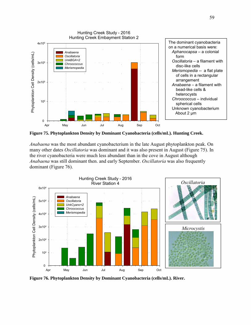
59



Phyt

opla

nkto

n C

ell D

ensi

ty (c

ells

/mL)

0

105

2x105

3x105

4x105

AnabaenaOscillatoriaUnkBGA<2ChroococcusMerismopedia

Figure 75. Phytoplankton Density by Dominant Cyanobacteria (cells/mL). Hunting Creek.

Anabaena was the most abundant cyanobacterium in the late August phytoplankton peak. On many other dates Oscillatoria was dominant and it was also present in August (Figure 75). In the river cyanobacteria were much less abundant than in the cove in August although Anabaena was still dominant then. and early September. Oscillatoria was also frequently dominant (Figure 76).



Phy

topl

ankt

on C

ell D

ensi

ty (c

ells

/mL)

0

104

2x104

3x104

4x104

5x104

6x104

AnabaenaOscillatoriaUnkCyano<2ChroococcusMerismopedia

Figure 76. Phytoplankton Density by Dominant Cyanobacteria (cells/mL). River.

The dominant cyanobacteria on a numerical basis were: Aphanocapsa – a colonial

form Oscillatoria – a filament with

disc-like cells Merismopedia -- a flat plate

of cells in a rectangular arrangement

Anabaena – a filament with bead-like cells & heterocysts

Chroococcus – individual spherical cells

Unknown cyanobacterium About 2 µm

Oscillatoria

Microcystis

60

Hunting CreekStudy - 2016Hunting Creek Embayment Station 2


Phy

topl

ankt

on C

ell D

ensi

ty (c

ells

/mL)

0

104

2.0x104

3.0x104

4.0x104

5.0x104

Pennate 1Pennate 2Pennate 3Discoid centricsMelosiraNavicula

Figure 77. Phytoplankton Density (#/mL) by Dominant Diatom Taxa. Hunting Creek.

Pennate diatoms were generally the greatest contributors to cell density at the Hunting Creek station AR2 (Figure 77). At AR2 diatoms were moderately abundant in April and early September. These times corresponded to elevated chlorophyll a levels. At the river station AR4 diatom densities were generally similar to those AR2 except in late June when large densities of two pennate diatoms were observed (Figure 78). These correlated with the large peak in chlorophyll observed at AR4 in late June

Hunting Creek Study - 2016 River Station 4


Phy

topl

ankt

on C

ell D

ensi

ty (c

ells

/mL)

0

5.0x104

105

1.5x105

2.0x105

Pennate 1Pennate 2Pennate 3Discoid centricsMelosiraNavicula

Figure 78. Phytoplankton Density (#/mL) by Dominant Diatom Taxa. River.

The most numerous non-diatom phytoplankters were:

Melosira – a filamentous centric diatom

Pennate 1 Pennate 2 Pennate 16 Navicula – a pennate Discoid centrics – mostly

Cyclotella

Melosira

61



Phy

topl

ankt

on C

ell D

ensi

ty (c

ells

/mL)

0

104

2.0x104

3.0x104

4.0x104

5.0x104

ChroomonasCryptomonasSpermatozoopsisChromulinaScenendesmusChlamydomonas

Figure 79. Phytoplankton Density (#/mL) by Dominant Other Taxa. Hunting Creek.

Phytoplankton species that were neither cyanobacteria nor diatoms were grouped together as “other” for these graphs; these included most numerous taxa of green algae, cryptophytes, euglenoids, and dinoflagellates. At both stations the cryptophytes Cryptomonas and Chroomonas were consistently the most numerous (Figure 79, 80).


Phy

topl

ankt

on C

ell D

ensi

ty (c

ells

/mL)

0

104

2x104

3x104

4x104

5x104

ChroomonasCryptomonasSpermatozoopsisChromulinaScenedesmusChlamydomonas


Figure 80. Phytoplankton Density (#/mL) by Dominant Taxa. River.

The most numerous other phytoplankton were: Cryptomonas – an ellip-

soidal, flagellated unicell Chroomonas – a

flagellated cryptomonad unicell

Spermatozoopsis – flagellated green unicell

Sennia – a flagellated unicellular cryptophyte

Pediastrum – a green alga Trachelomonas – a spherical euglenoid Scenedesmus – a green alga Coelastrum – a green alga

62



Phy

topl

ankt

on B

iovo

lum

e (

m3 /m

L)

0

2x107

4x107

6x107

8x107


Figure 81. Phytoplankton Biovolume (um3/mL) by Major Groups. Hunting Creek.

In the cove diatoms were dominant in biovolume in most samples (Figure 81). The highest biovolumes generally coincided with elevated chlorophyll a levels: April and late August-early September. In the river, diatoms were overwhelming in their dominance (Figure 82). Cryptophytes and other algae made substantial contributions on some dates.



Phy

topl

ankt

on B

iovo

lum

e (

m3 /m

L)

0

2.0x107

4.0x107

6.0x107


Figure 82. Phytoplankton Biovolume (um3/mL) by Major Groups. River.

Total phytoplankton biovolume can be broken down into groups: Cyano – cyanobacteria

(“blue-green” algae) Greens – green algae Diatoms – includes both

centric and pinnate Cryptos – cryptophytes Other – includes euglenoids,

chrysophytes, and dinoflagellates

While dominating cell density, cyanobacteria typically make up a much smaller portion of phytoplankton biovolume. Diatoms generally are dominant.

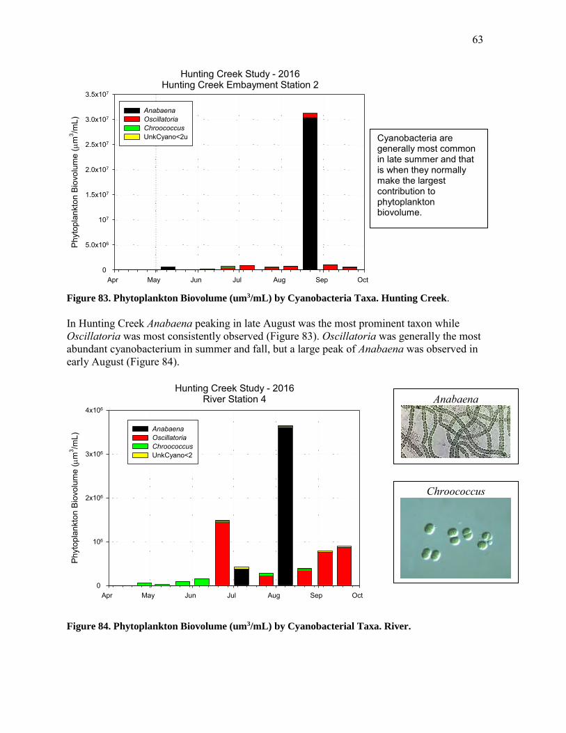
63



Phy

topl

ankt

on B

iovo

lum

e (

m3 /m

L)

0

5.0x106

107

1.5x107

2.0x107

2.5x107

3.0x107

3.5x107

AnabaenaOscillatoriaChroococcusUnkCyano<2u

Figure 83. Phytoplankton Biovolume (um3/mL) by Cyanobacteria Taxa. Hunting Creek. In Hunting Creek Anabaena peaking in late August was the most prominent taxon while Oscillatoria was most consistently observed (Figure 83). Oscillatoria was generally the most abundant cyanobacterium in summer and fall, but a large peak of Anabaena was observed in early August (Figure 84).



Phy

topl

ankt

on B

iovo

lum

e (

m3 /m

L)

0

106

2x106

3x106

4x106

AnabaenaOscillatoriaChroococcusUnkCyano<2

Figure 84. Phytoplankton Biovolume (um3/mL) by Cyanobacterial Taxa. River.

Cyanobacteria are generally most common in late summer and that is when they normally make the largest contribution to phytoplankton biovolume.

Anabaena

Chroococcus

64


Phy

topl

ankt

on B

iovo

lum

e (

m3 /m

L)

0

107

2x107

3x107

4x107

5x107

MelosiraPennate 2SurrirellaDiscoid centricsPennate 1Rhoicosphaenia


Figure 85. Phytoplankton Biovolume (um3/mL) by Dominant Diatom Taxa. Hunting Creek.

Melosira was the overwhelming dominant in biovolume in late April and again in late May, but disappeared thereafter (Figure 85). In the river, Melosira was dominant early and late, but pennate diatoms dominated during the late June peak in phytoplankton chlorophyll (Figure 86).



Phy

topl

ankt

on B

iovo

lum

e (

m3 /m

L)

0

107

2.0x107

3.0x107

4.0x107

5.0x107

MelosiraPennate 2SurrirellaDiscoid centricsPennate 1Rhoicosphaenia

Figure 86. Phytoplankton Biovolume (um3/mL) by Dominant Diatom Taxon. River.

Discoid Centrics

Melosira

65



Phy

topl

ankt

on B

iovo

lum

e (

m3 /m

L)

0

5.0x106

107

1.5x107

2.0x107

2.5x107

3.0x107

OocystisTrachelomonasCosmariumCryptomonasEuglenaSpermatozoopsis

Figure 87. Phytoplankton Biovolume (um3/mL) by Dominant Other Taxa. Hunting Creek.

The cryptophyte Cryptomonas was a strong contributor to biovolume in Hunting Creek in late April (Figure 87). The green alga Cosmarium was dominant in late July and the green alga Oocystic was increasingly abundant in the fall. In the river Cryptomonas was much less dominant (Figure 88). In the river Trachelomonas and Cryptomonas were typically dominant for most of the year.



Phy

topl

ankt

on B

iovo

lum

e (

m3 /m

L)

0

5.0x106

107

1.5x107

2.0x107

OocystisTrachelomonasCosmariumCryptomonasEuglenaSpermatozoopsis

Figure 88. Phytoplankton Biovolume (um3/mL) by Dominant Other Taxon. River.

Discoid Centrics

Euglena

http://images.google.com/imgres?imgurl=http://arnica.csustan.edu/Biol1010/classification/euglena.JPG&imgrefurl=https://eapbiofield.wikispaces.com/PR%2B9%2BClassification%2BMolly?f%3Dprint&usg=__tLBaDd4tXa7bZM2XfNz6mt18asE=&h=346&w=548&sz=110&hl=en&start=17&um=1&tbnid=adlA1Fh4o0jTPM:&tbnh=84&tbnw=133&prev=/images?q%3Deuglena%26hl%3Den%26rlz%3D1T4DIUS_enUS317US317%26sa%3DN%26um%3D1

66

E. Zooplankton – 2016

Hunting Creek Study - 2016 - Station 2


Rot

ifers

(#/L

)

0

200

400

600

800

1000

1200

1400

1600

1800

BrachionusKeratellaMonostylaPloesomaPolyarthraSynchaeta

Figure 89. Rotifer Density by Dominant Taxa (#/L). Hunting Creek.

In Hunting Creek, rotifers exhibited a minor peak in early June and a major peak in late August (Figure 89). Brachionus was generally dominant with a strong showing from Ploesoma on many dates and Monostyla in late August. In the river Brachionus and Ploesoma were most important with Keratella and Polyarthra making significant contributions. (Figure 90). Rotifer densities at the two site were similar except in late August.

Hunting Creek Study - 2016 - Station 4


Rot

ifers

(#/L

)

0

100

200

300

400

500

600

BrachionusKeratellaMonostylaPloesomaPolyarthraSynchaeta

Figure 90. Rotifer Density by Dominant Taxa (#/L). River.

Brachionus (c. 50 um)

Conochilidae

Brachionus (Sta 7, RCJ)

Keratella (Sta 7, RCJ)

67



Bo

sm

ina

(#/L

)

0

50

100

150

200

250Station 2Station 4

Figure 91. Bosmina Density by Station (#/L).

In 2016 the small cladoceran Bosmina was generally present at low densities at both stations (Figure 91). The exception were elevated values at AR2 in late April and early June Diaphanosoma, typically the most abundant larger cladoceran in Gunston Cove, was present at almost identical values at the two sampling stations, peaking at about 600/m3 (Figure 92).



Dia

ph

an

os

om

a (#

/m3 )

0

100

200

300

400

500

600


Figure 92. Diaphanosoma Density by Station (#/m3).

Bosmina is a small-bodied cladoceran, or “waterflea”, which is common in lakes and freshwater tidal areas. It is typically the most abundant cladoceran with maximum numbers generally about 100-1000 animals per liter. Due to its small size and relatively high abundances, it is enumerated in the micro-zooplankton samples. Bosmina can graze on smaller phytoplankton cells, but can also utilize some cells from colonies by knocking them loose.

Diaphanosoma is the most abundant larger cladoceran found in the tidal Potomac River. It generally reaches numbers of 1,000-10,000 per m3 (which would be 1-10 per liter). Due to their larger size and lower abundances, Diaphanosoma and the other cladocera are enumerated in the macrozooplankton samples. Diaphanosoma prefers warmer temperatures than some cladocera and is often common in the summer.

68



Da

ph

nia

(#/m

3 )

0

100

200

300

400

500

600

700

800

900


Figure 93. Daphnia Density by Station (#/m3).

Daphnia was moderately abundant in the study area in late June 2016, but was rare for the rest of the year. Again values were almost identical at the two stations (Figure 93). Ceriodaphnia was also restricted to significant numbers on the one date in late June (Figure 94). Peak levels were 400-500/m3.



Ce

rio

da

ph

nia

(#/m

3 )

0

100

200

300

400

500

600

Station 2Station 4

Figure 94. Ceriodaphnia Density by Station (#/m3).

Daphnia, the common waterflea, is one of the most efficient grazers of phytoplankton in freshwater ecosystems. In the tidal Potomac River it is present, but has not generally been as abundant as Diaphanosoma. It is typically most common in spring. Size? Picture?

Ceriodaphnia, another common large-bodied cladoceran, is usually present in numbers similar to Daphnia. Like all waterfleas, the juveniles look like miniature adults and grow through a series of molts to a larger size and finally reach reproductive maturity. Most reproduction is asexual except during stressful environmental conditions.

69



Sid

a (#

/m3 )

0

100

200

300

400

500

600


Figure 95. Sida Density by Station (#/m3).

Sida was yet another cladoceran whose values peaked in late June at nearly identical values at both stations (Figure 95). It was also present in lower numbers in the fall. Leptodora, the large cladoceran predator, peaked in early June in Hunting Creek and in late June at the rier mainstem site AR4 (Figure 96).



Le

pto

do

ra (#

/m3 )

0

100

200

300

400

Station 2Station 4

Figure 96. Leptodora Density by Station (#/m3).

Moinadaphnia is another waterflea that is often observed in the tidal Potomac River. Like the other cladocera mentioned so far, Moinadaphnia grazes on phytoplankton to obtain its food supply.

Leptodora is substantially larger than the other cladocera mentioned. Also different is its mode of feeding – it is a predator on other zooplankton. It normally occurs for brief periods in the late spring or early summer.

70



Ca

mp

toc

erc

us (#

/m3 )

0

100

200

300

400


Figure 97. Camptocercus Density by Station (#/m3). (photo: L. Birsa from HC samples) Camptocercus is a taxon associated with SAV (Figure 97). It was found almost exclusively at the Hunting Creek embayment (AR2), peaking in early August. Macrothricidae, another group associated with SAV, were also present mainly at AR2 and were recorded mostly in early September (Figure 98).



Mac

roth

ricid

ae (#

/m3 )

0

100

200

300

400


Figure 98. Macrothricid Density by Station (#/m3). (photo: L. Birsa from HC samples)

71



Cop

epod

nau

plii

(#/L

)

0

100

200

300

400

500

600

Station 2Station 4

Figure 99. Copepod Nauplii Density by Station (#/L).

Copepod nauplii were present at elevated levels at AR2 in April and in June reaching 500/L (Figure 99). Levels in the river also peaked in late June at a lower level of about 200/L. Eurytemora was quite abundant in Hunting Creek in April and early May, but declined thereafter. In the river, densities increased strongly in June reaching a very large peak of 28,000/m3 in late June (Figure 100).



Eu

ryte

mo

ra (#

/m3 )

0

2000

4000

6000

8000

1000026000

28000


Figure 100. Eurytemora Density by Station (#/m3).

Copepod eggs hatch to form an immature stage called a nauplius. The nauplius is a larval stage that does not closely resemble the adult and the nauplii of different species of copepods are not easily distinguished so they are lumped in this study. Copepods go through 5 naupliar molts before reaching the copepodid stage which is morphologically very similar to the adult. Because of their small size and high abundance, copepod nauplii are enumerated in the micro-zooplankton samples.

Eurytemora affinis is a large calanoid copepod characteristic of the freshwater and brackish areas of the Chesapeake Bay. Eurytemora is a cool water copepod which often reaches maximum abundance in the late winter or early spring. Included in this graph are adults and those copepodids that are recognizable as Eurytemora.

72



Dia

pto

mu

s (#

/m3 )

0

500

1000

1500


Figure 101. Diaptomus Density by Station (#/m3).

Diaptomus was almost exclusively found in Hunting Creek where it reached a substantial peak of nearly 2000/m3 in late June (Figure 101). Cyclopoid copepods were present at relatively low numbers at both sites (Figure 102).



Cyc

lopo

id C

opep

ods

(#/m

3 )

0

100

200

300

400

500

Station 2Station 4

Figure 102. Cyclopoid Copepods by Station (#/m3).

Diaptomus pallidus is a calanoid copepod often found in moderate densities in the Gunston Cove area. Diaptomus is an efficient grazer of algae, bacteria, and detrital particles in freshwater ecosystems Included in this graph are adults and those copepodids that are recognizable as Diaptomus.

Cyclopoids are the other major group of planktonic copepods. Cyclopoids feed on individual particles suspended in the water including small zooplankton as well as phytoplankton. In this study we have lumped all copepodid and adult cyclopoids together.

73

F. Ichthyoplankton – 2016 We collected 14 samples (7 at Station AR2 and 7 at Station AR4) during the months April through July and found an average total larval density of 338 larvae per 10 m3 (Table 4), which is an order of magnitude less than last year. The dominant species was Gizzard Shad (Dorosoma cepedianum) with an average larval density of 111 larvae per 10m3. The taxon Clupeidae had the second highest density with 88 larvae per 10m3, which is comprised of clupeids (Alosa or Dorosoma sp.) that could not be identified to a lower taxonomic level. Alosa aestivalis (Blueback Herring) and Alosa pseudoharengus (Alewife) were present in relative high densities as well: 46 and 39 larvae per 10m3 on average respectively. Other clupeids present that could positively be identified to the species level are Hickory Shad at an average of 5 per 10m3, and American Shad at 1 larva per 10m3. A different taxon with relatively high representation is Inland Silverside (Menidia beryllina) with an average of 10 larvae per 10m3. Fishes of the genus Morone (which includes White Perch and Striped Bass) were relatively abundant as well, with an average of 7 larvae per 10m3 identified to the genus level, plus 4.3 positively identified White Perch, and 0.6 Striped Bass larvae per 10m3. Table 4. The average larval density (#/10m3) in Hunting Creek (AR2) and the Potomac River (AR4) in 2016.

Taxon Species AR2 AR4 Average

Alosa aestivalis Blueback Herring 51.75 39.79 45.77 Alosa mediocris Hickory Shad 7.83 1.81 4.82 Alosa pseudoharengus Alewife 42.24 36.28 39.26 Alosa sapidissima American Shad 1.65 0.32 0.99 Carassius auratus Goldfish 0.00 0.30 0.15 Carpiodes cyprinus Quillback 0.78 0.00 0.39 Dorosoma cepedianum Gizzard Shad 150.53 71.01 110.77 Etheostoma olmstedi Tessellated Darter 0.00 0.13 0.07 Fundulus sp. Killifishes 0.20 0.00 0.10 Lepomis cyanellus Green Sunfish 0.41 0.00 0.20 Lepomis gibbosus Pumpkinseed 1.30 0.32 0.81 Centrarchidae species Centrarchids 0.00 0.13 0.07 Menidia beryllina Inland Silverside 16.71 3.64 10.18 Menidia species Unidentified Silverside 1.93 0.67 1.30 Morone americana White perch 6.93 1.67 4.30 Morone saxatilis Striped bass 0.00 1.10 0.55 Morone sp. Morone species 10.83 3.28 7.05 Notropis hudsonius Spottail Shiner 0.39 0.00 0.19 Perca flavescens Yellow Perch 0.65 0.00 0.32 Unidentified Clupeidae Unidentified Clupeid 81.52 93.98 87.75 Eggs Eggs 6.91 10.89 8.90 Unidentified Unidentified 22.24 6.36 14.30

74

Figure 103. Average Density of clupeid larvae per 10m3.

Clupeid larvae in Figure 103 include Blueback Herring, Hickory Shad, Alewife, American Shad and Gizzard Shad. These have similar spawning patterns so they are lumped into one group for this analysis. Clupeids were present in the sample at the end of April (first sampling date was April 27), increased to over 200 larvae per 10 m3 in early June, and decreased again at the end of June (Figure 103). Of these clupeids, Alewife and Blueback Herring are the two species that make up river herring, of which we describe the spawning population at the end of this report. White Perch and Striped Bass (Morone spp.) larvae attained highest density on average just over 10 larvae per 10m3 at the start of sampling in April (Figure 104), and completely disappeared from the samples in July. The group of larvae that are not positively identified clupeids or Morone species are dominated by unidentified larvae (Figure 105). Highest densities of unidentified larvae were found at the start of May with a second peak at the start of June. The unidentified larvae were not intact unknown species, but larvae too mangled for proper identification. Because of the high density of clupeid larvae, most unidentified larvae are likely to be clupeids as well.

75

Figure 104. Density of Morone sp. (white perch and striped bass) per 10m3.

Figure 105. Density of other larvae per 10m3.

76

G. Adult and juvenile fishes – 2016 Trawls Trawl sampling was conducted between April 28 and September 7 at AR3 and AR4 (Figure 1c). A total of 98 fishes comprising at least 14 species were collected with trawls (Table 5). Both the abundance and diversity is lower than previous years. Collections were dominated by Blueback Herring (30%). The second most abundant species caught was American Shad (19%). Other abundant species (annual total >5%) included: Alewife (12%), Pumpkinseed (6%), and Common Carp (5%). Other species were observed at lower abundances (Tables 5 and 6). An interesting find was the collection of two native catfishes (White and Brown bullhead), which have seen declining abundances since the invasion of Blue Catfish. Table 5. Adult and juvenile fish collected by trawling. Hunting Creek - 2016

Species Common name Abundance % total Alosa aestivalis Blueback Herring 29 29.59 Alosa pseudoharengus Alewife 12 12.24 Alosa sapidissima American Shad 19 19.39 Alosa sp. Herring or shad 7 7.14 Ameiurus catus White Bullhead 1 1.02 Ameiurus nebulosus Brown Bullhead 1 1.02 Cyprinus carpio Common Carp 5 5.10 Etheostoma olmstedi Tessellated Darter 3 3.06 Fundulus diaphanus Banded Killifish 1 1.02 Ictalurus furcatus Blue Catfish 1 1.02 Lepomis gibbosus Pumpkinseed 6 6.12 Lepomis sp. Sunfishes 4 4.08 Micropterus salmoides Largemouth Bass 1 1.02 Morone americana White Perch 3 3.06 Notropis hudsonius Spottail Shiner 2 2.04 Perca flavescens Yellow Perch 3 3.06 Total 98 100

Trawling collects fish that are located in the open water near the bottom. Due to the shallowness of Hunting Creek, the volume collected is a substantial part of the water column. However, in the river channel, the near bottom habitat through which the trawl moves is only a small portion of the water column. Fishes tend to concentrate near the bottom or along shorelines rather than in the upper portion of the open water.

77

Table 6. Adult and juvenile fish collected by trawling. Hunting Creek study - 2016

Species Common Name 4/28 5/12 5/26* 6/9 6/22 7/6 7/20 8/10 8/24 9/7 Total

Alosa aestivalis Blueback Herring 0 0 0 0 0 0 0 29 0 29 Alosa pseudoharengus Alewife 0 0 0 0 0 0 0 12 0 12 Alosa sapidissima American Shad 0 0 0 0 0 0 0 19 0 19 Alosa sp. Herring or shad 0 0 1 0 6 0 0 0 0 7 Ameiurus catus White Bullhead 0 0 0 0 0 1 0 0 0 1 Ameiurus nebulosus Brown Bullhead 0 1 0 0 0 0 0 0 0 1 Cyprinus carpio Common Carp 0 0 0 0 5 0 0 0 0 5 Etheostoma olmstedi Tessellated Darter 0 0 1 1 1 0 0 0 0 3 Fundulus diaphanus Banded Killifish 0 1 0 0 0 0 0 0 0 1 Ictalurus furcatus Blue Catfish 0 0 0 0 0 1 0 0 0 1 Lepomis gibbosus Pumpkinseed 0 4 1 0 1 0 0 0 0 6 Lepomis sp. Sunfishes 0 0 0 0 4 0 0 0 0 4 Micropterus salmoides Largemouth Bass 0 0 0 0 1 0 0 0 0 1 Morone americana White Perch 1 0 0 0 0 2 0 0 0 3 Notropis hudsonius Spottail Shiner 0 2 0 0 0 0 0 0 0 2 Perca flavescens Yellow Perch 1 2 0 0 0 0 0 0 0 3 Total 2 10 3 1 18 4 0 60 0 98

*Trawls could not be completed on 5/26 due to engine problems.

78

The highest catch occurred on August 24, and was due to the high abundance of alosas in that trawl sample (Tables 6). In 2016, most catches occurred in AR4, while we usually have higher catches in AR3 (Table 7). There were four more trawls in AR4 than AR3 this year, because trawling at AR3 became impossible in the second half of the sampling season (Table 1), and presence of SAV made trawling difficult during the days the trawl was performed as well. The catch at station 4 was similar to previous years with 72 individuals from 9 species. At Station 3 only 26 individuals were collected, but there was a slightly higher diversity than in AR4 with 11 species. Table 7. Adult and juvenile fish collected by trawling. Hunting Creek study - 2016 Species Common name Station 3 Station 4 Alosa aestivalis Blueback Herring 0 29 Alosa pseudoharengus Alewife 0 12 Alosa sapidissima American Shad 0 19 Alosa sp. Herring or shad 1 6 Ameiurus catus White Bullhead 0 1 Ameiurus nebulosus Brown Bullhead 1 0 Cyprinus carpio Common Carp 5 0 Etheostoma olmstedi Tessellated Darter 2 1 Fundulus diaphanus Banded Killifish 1 0 Ictalurus furcatus Blue Catfish 0 1 Lepomis gibbosus Pumpkinseed 5 1 Lepomis sp. Sunfishes 4 0 Micropterus salmoides Largemouth Bass 1 0 Morone americana White Perch 1 2 Notropis hudsonius Spottail Shiner 2 0 Perca flavescens Yellow Perch 3 0 Total 26 72

Only 3 White Perch were collected, which was the dominant species in previous years. High dominance of White Perch at AR3 was also for a large part responsible for the large catch in AR3 in previous years. Looking at species by dominance (Figure 106A and B), Alosas were the most common species in 2016, while carp and centrarchids were most common in AR3. The month with the most catches was August, when most Alosas were collected (table 6).

White perch (Morone americana) is the dominant species in Hunting Creek, and continues to be an important commercial and popular game fish. Adults grow to over 30 cm long. Sexual maturity begins the second year at lengths greater than 9 cm. As juveniles they feed on zooplankton and macrobenthos, but as they get larger consume fish as well.

79

Figure 106A and B. Pareto chart of adult and juvenile fishes collected by trawling. Dominant species by station in total abundance and cumulative percentage of total for AR3 (top) and AR4 (bottom).

Spottail shiner (Notropis hudsonius is a common fish in the open waters of Hunting Creek. Spawning occurs throughout the warmer months. It reaches sexual maturity at about 5.5 cm and may attain a length of 10 cm. They feed primarily on benthic invertebrates and occasionally on algae and plants.

80

Seines

Seine sampling was conducted between April 28 and September 7 at AR5 and AR6. As planned, one sampling trip per month was performed in April and September, and two sampling trips per month from May to August. The two seines stations (AR5 and AR6; Figure 1) were selected as sites with shallow sloping shorelines that would enable us to tow a beach seine. The net was towed up onto the beach unless high water completely submerged the beach. In those cases, the net was towed into the boat. Table 8. Adult and juvenile fish collected by seining. Hunting Creek study – 2016 Species Common name Abundance % Total Alosa sp. Herring or Shad 4 0.23 Ameiurus nebulosus Brown Bullhead 2 0.12 Cyprinus carpio Common Carp 2 0.12 Fundulus diaphanus Banded Killifish 1386 81.24 Fundulus heteroclitus Mummichog 16 0.94 Hybognathus regius Eastern Silvery Minnow 2 0.12 Lepomis auritus Redbreast Sunfish 2 0.12 Lepomis gibbosus Pumpkinseed 5 0.29 Lepomis macrochirus Bluegill 8 0.47 Lepomis microlophus Redear Sunfish 2 0.12 Lepisosteus osseus Longnose Gar 1 0.06 Lepomis sp. Sunfishes 23 1.35 Menidia beryllina Inland Silverside 209 12.25 Micropterus dolomieu Smallmouth Bass 6 0.35 Micropterus salmoides Largemouth Bass 4 0.23 Morone americana White Perch 16 0.94 Morone saxatilis Striped Bass 1 0.06 Notemigonus crysoleucas Golden Shiner 2 0.12 Notropis hudsonius Spottail Shiner 11 0.64 Perca flavescens Yellow Perch 4 0.23 Total 1706 100

A total of 20 seine samples were conducted (10 per station), comprising 1706 fishes of at least 20 species (Table 8). By far the most dominant species in seine catches was banded Killifish (81.24%). This is similar to last year, although the total number of individuals is lower. Other species that were relatively abundant were Inland Silverside (12.25%), and sunfishes (1.35%). Other species occurred at low abundances (Table 8). Banded Killifish was present and dominant in all months sampled (Table 9; Figure 107A&B). The most productive month was June due to the high numbers of Banded Killifish present that month. In both stations the high majority of all fish collected was

81

banded killifish (Table 10). The total number of individuals in AR6 was almost 3 times higher than AR5. The Pareto charts of AR5 and AR6 (Figure 108A&B) indicate with very shallow slopes of the cumulative percent of the catch that banded killifish is highly dominant, with relatively small contributions of other species. Other species with relatively high total abundance (> 10 specimens) were Inland Silverside, sunfishes, Mummichog, White Perch, and Spottail Shiner.

Figure 107A and B. Adult and juvenile fish collected by seining. Dominant species by month in percentage of total (A) and total abundance (B)

0%10%20%30%40%50%60%70%80%90%

100%

0

100

200

300

400

500

600

700

800Fundulus diaphanus

Menidia beryllina

Lepomis species

FundulusheteroclitusMorone americana

Other

82

Table 9. Adult and juvenile fish collected by seining. Hunting Creek study - 2016

Species Common Name 4/28 5/12 5/26 6/9 6/22 7/6 7/20 8/10 8/24 9/7 Total

Alosa species Unidentified Herring or shad 4 0 0 0 0 0 0 0 0 0 4 Ameiurus catus White Bullhead 0 0 0 0 0 0 0 0 0 0 0 Ameiurus nebulosus Brown Bullhead 0 0 0 0 0 1 0 0 0 1 2 Cyprinus carpio Carp 0 0 1 0 0 0 1 0 0 0 2 Fundulus diaphanus Banded Killifish 174 362 137 608 15 28 11 21 25 5 1386 Fundulus heteroclitus Mummichog 0 7 2 3 0 4 0 0 0 0 16 Hybognathus regius Eastern Silvery Minnow 0 0 1 1 0 0 0 0 0 0 2 Lepomis auritus Redbreast Sunfish 0 0 0 0 1 1 0 0 0 0 2 Lepomis gibbosus Pumpkinseed 0 1 0 0 0 0 0 0 0 4 5 Lepomis macrochirus Bluegill 0 1 1 0 0 0 0 2 4 0 8 Lepomis microlophus Redear Sunfish 0 0 0 0 0 0 0 2 0 0 2 Lepisosteus osseus Longnose Gar 0 0 0 0 1 0 0 0 0 0 1 Lepomis species Unidentified Sunfish 0 0 0 0 0 0 14 9 0 0 23 Menidia beryllina Inland Silverside 5 64 3 133 0 2 0 2 0 0 209 Micropterus dolomieu Small-mouth Bass 0 0 0 0 0 1 1 2 2 0 6 Micropterus salmoides Large-mouth Bass 0 2 1 0 0 0 0 0 0 1 4 Morone americana White Perch 5 0 1 0 2 0 1 5 0 2 16 Morone saxatilis Striped Bass 0 0 1 0 0 0 0 0 0 0 1 Notemigonus crysoleucas Golden Shiner 0 1 1 0 0 0 0 0 0 0 2 Notropis hudsonius Spottail Shiner 9 0 2 0 0 0 0 0 0 0 11 Perca flavescens Yellow Perch 0 2 0 0 0 0 0 2 0 0 4 Total 197 440 151 745 19 37 28 45 31 13 1706

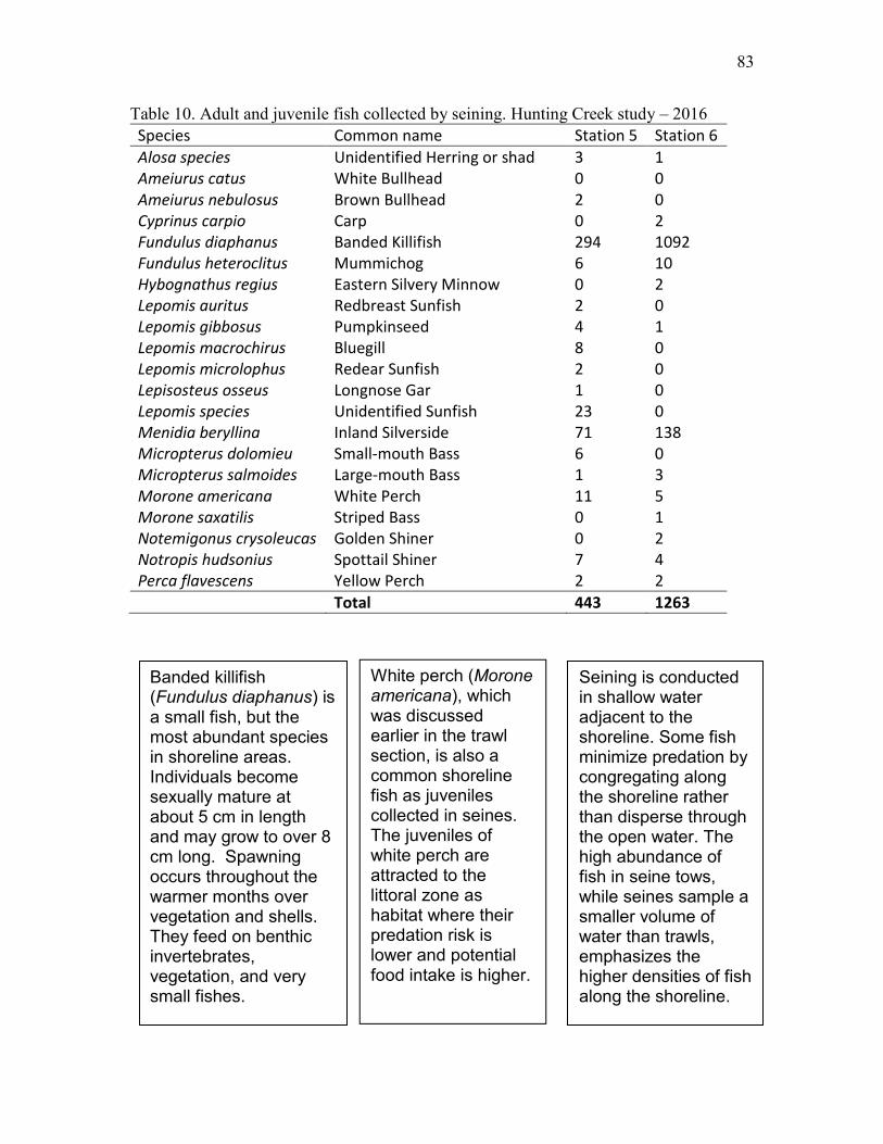
83

Table 10. Adult and juvenile fish collected by seining. Hunting Creek study – 2016 Species Common name Station 5 Station 6

Alosa species Unidentified Herring or shad 3 1 Ameiurus catus White Bullhead 0 0 Ameiurus nebulosus Brown Bullhead 2 0 Cyprinus carpio Carp 0 2 Fundulus diaphanus Banded Killifish 294 1092 Fundulus heteroclitus Mummichog 6 10 Hybognathus regius Eastern Silvery Minnow 0 2 Lepomis auritus Redbreast Sunfish 2 0 Lepomis gibbosus Pumpkinseed 4 1 Lepomis macrochirus Bluegill 8 0 Lepomis microlophus Redear Sunfish 2 0 Lepisosteus osseus Longnose Gar 1 0 Lepomis species Unidentified Sunfish 23 0 Menidia beryllina Inland Silverside 71 138 Micropterus dolomieu Small-mouth Bass 6 0 Micropterus salmoides Large-mouth Bass 1 3 Morone americana White Perch 11 5 Morone saxatilis Striped Bass 0 1 Notemigonus crysoleucas Golden Shiner 0 2 Notropis hudsonius Spottail Shiner 7 4 Perca flavescens Yellow Perch 2 2

Total 443 1263

White perch (Morone americana), which was discussed earlier in the trawl section, is also a common shoreline fish as juveniles collected in seines. The juveniles of white perch are attracted to the littoral zone as habitat where their predation risk is lower and potential food intake is higher.

Seining is conducted in shallow water adjacent to the shoreline. Some fish minimize predation by congregating along the shoreline rather than disperse through the open water. The high abundance of fish in seine tows, while seines sample a smaller volume of water than trawls, emphasizes the higher densities of fish along the shoreline.

Banded killifish (Fundulus diaphanus) is a small fish, but the most abundant species in shoreline areas. Individuals become sexually mature at about 5 cm in length and may grow to over 8 cm long. Spawning occurs throughout the warmer months over vegetation and shells. They feed on benthic invertebrates, vegetation, and very small fishes. Species Common

name Station 5

Station 6

Alosa species

Unidentified Herring or shad 3 1

Ameiurus White

84

Figure 108. A and B. Pareto chart of adult and juvenile fishes collected by seining.

Dominant species by station in total abundance and cumulative percentage of total

for Station 5 (top) and Station 6 (bottom).

85

Fyke Nets Both fyke nets were set near AR3 (Figure 1c), and the total fyke nets catch was higher than the total trawl catch at AR3 (316 versus 98). We were able to continue our fyke net sampling when SAV growth had rendered trawling impossible. Fyke nets were set from May 12 to September 7. Except for the first sampling date in April, fyke nets were set during every sampling trip throughout the season (Table 1). In a total of 18 samples (9 per fyke net), we collected 316 individual fishes from at least 15 species. As in the seine collections, the dominant species was Banded Killifish, which represented 49% of the total abundance (Table 11). The percent dominance was distributed a little more evenly over the species collected in fyke nets, and 10 other species had a dominance of at least more than 1 %. Species of which at least 10 individuals were collected are Lepomis sp. (18.35% of total), White Perch (12%), Bluegill (3.8%), and Pumpkinseed (3.48%). Table 11. Adult and juvenile fish collected by fyke nets. Hunting Creek study – 2016

Species Common Name Abundance

%

Total

Alosa sp. Herring or shad 1 0.32 Ameiurus catus White Bullhead 1 0.32 Carassius auratus Goldfish 9 2.85 Cyprinus carpio Common Carp 7 2.22 Etheostoma olmstedi Tessellated Darter 5 1.58 Fundulus diaphanus Banded Killifish 156 49.37 Hybognathus regius Eastern Silvery Minnow 2 0.63 Lepomis gibbosus Pumpkinseed 11 3.48 Lepomis macrochirus Bluegill 12 3.80 Lepomis microlophus Redear Sunfish 6 1.90 Lepomis sp. Unidentified Sunfish 58 18.35 Menidia beryllina Inland Silverside 1 0.32 Morone americana White Perch 38 12.03 Morone saxatilis Striped Bass 4 1.27 Notropis hudsonius Spottail Shiner 4 1.27 Pomoxis nigromaculatus Black Crappie 1 0.32 Total 316 100.00

The highest abundance occurred in the second half of the sampling season, with the highest catch occurring in the month of July and second highest catch in August (Table 12). All species collected had higher abundances in July and August than May and June, which makes the fyke nets a great addition to the sampling gear, since the trawl cannot be towed anymore in those months.

86

Table 12. Adult and juvenile fish collected by fyke nets. Hunting Creek study - 2016 Species Common Name 4/28* 5/12 5/26 6/9 6/22 7/6 7/20 8/10 8/24 9/7 Total

Alosa sp. Herring or shad 1 0 0 0 0 0 0 0 0 1

Ameiurus catus White Bullhead 0 0 0 0 0 0 0 0 1 1

Carassius auratus Goldfish 0 0 0 0 0 6 0 2 1 9

Cyprinus carpio Common Carp 0 0 0 0 5 0 2 0 0 7

Etheostoma olmstedi Tessellated Darter 0 0 0 0 2 0 0 1 2 5

Fundulus diaphanus Banded Killifish 0 0 5 14 13 68 10 29 17 156

Hybognathus regius Eastern Silvery Minnow 0 0 0 0 1 0 0 1 0 2

Lepomis gibbosus Pumpkinseed 2 0 4 3 0 0 1 1 0 11

Lepomis macrochirus Bluegill 0 1 0 0 0 2 5 2 2 12

Lepomis microlophus Redear Sunfish 2 0 0 0 4 0 0 0 0 6

Lepomis sp. Unidentified Sunfish 0 0 0 0 0 5 14 18 21 58

Menidia beryllina Inland Silverside 0 0 1 0 0 0 0 0 0 1

Morone americana White Perch 1 0 2 4 0 5 3 16 7 38

Morone saxatilis Striped Bass 0 0 0 0 0 3 0 1 0 4

Notropis hudsonius Spottail Shiner 0 0 0 1 1 0 0 2 0 4

Pomoxis nigromaculatus Black Crappie 1 0 0 0 0 0 0 0 0 1

Total 7 1 12 22 26 89 35 73 51 316

*no fyke nets were set during the first sampling day due to logistical issues.

87

While both fyke nets are close to each other and sample the littoral zone, the fyke net further from shore collects more open water species such as white perch (Table 13). The total catch was more than twice as high in Fyke Near than Fyke Far (217 versus 99, Table 13), which was mostly due to the high abundance of Banded Killifish (124) collected in Fyke Near. The pareto charts show that the order of dominance was strikingly similar between the two fyke nets, while the evenness was higher in Fyke Far (Figure 109A and B). Overall the evenness in the Fyke collections was high in the fyke nets, with representation of several species as a significant portion of the total catch (Figure 110A and B). Table 13. Adult and juvenile fish collected by fyke nets. Hunting Creek study – 2016

Species Common Name Fyke Near Fyke Far

Alosa species Unidentified Herring or shad 1 0

Ameiurus catus White Bullhead 0 1

Carassius auratus Goldfish 8 1

Cyprinus carpio Carp 5 2

Etheostoma olmstedi Tessellated Darter 3 2

Fundulus diaphanus Banded Killifish 124 32

Hybognathus regius Eastern Silvery Minnow 0 2

Lepomis gibbosus Pumpkinseed 8 3

Lepomis macrochirus Bluegill 11 1

Lepomis microlophus Redear Sunfish 5 1

Lepomis species Unidentified Sunfish 33 25

Menidia beryllina Inland Silverside 1 0

Morone americana White Perch 13 25

Morone saxatilis Striped Bass 2 2

Notropis hudsonius Spottail Shiner 3 1

Pomoxis nigromaculatus Black Crappie 0 1

Total 217 99

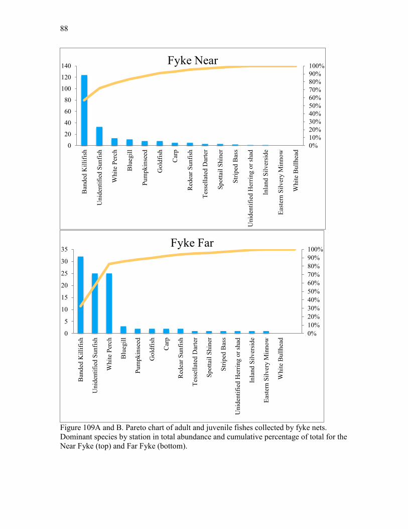
88

Figure 109A and B. Pareto chart of adult and juvenile fishes collected by fyke nets. Dominant species by station in total abundance and cumulative percentage of total for the Near Fyke (top) and Far Fyke (bottom).

0%10%20%30%40%50%60%70%80%90%100%

0

20

40

60

80

100

120

140

Ban

ded

Kill

ifish

Uni

dent

ified

Sun

fish

Whi

te P

erch

Blu

egill

Pum

pkin

seed

Gol

dfis

h

Car

p

Red

ear S

unfis

h

Tess

ella

ted

Dar

ter

Spot

tail

Shin

er

Strip

ed B

ass

Uni

dent

ified

Her

ring

or sh

ad

Inla

nd S

ilver

side

East

ern

Silv

ery

Min

now

Whi

te B

ullh

ead

Fyke Near

0%10%20%30%40%50%60%70%80%90%100%

0

5

10

15

20

25

30

35

Ban

ded

Kill

ifish

Uni

dent

ified

Sun

fish

Whi

te P

erch

Blu

egill

Pum

pkin

seed

Gol

dfis

h

Car

p

Red

ear S

unfis

h

Tess

ella

ted

Dar

ter

Spot

tail

Shin

er

Strip

ed B

ass

Uni

dent

ified

Her

ring

or sh

ad

Inla

nd S

ilver

side

East

ern

Silv

ery

Min

now

Whi

te B

ullh

ead

Fyke Far

89

Figure 110A and B. Adult and juvenile fish collected by fyke nets. Dominant species by month in percentage of total (A) and total abundance (B).

0

0.1

0.2

0.3

0.4

0.5

0.6

0.7

0.8

0.9

1

0

20

40

60

80

100

120

Banded KillifishUnidentified SunfishWhite PerchBluegillPumpkinseedOther

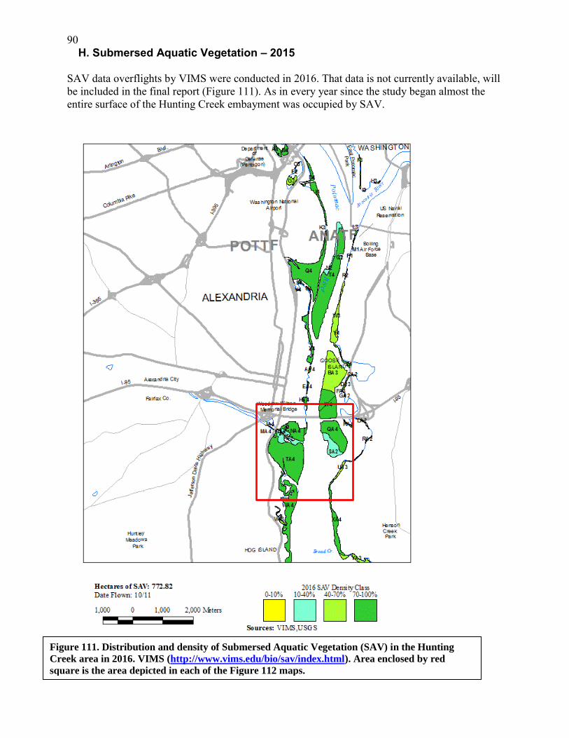
90 H. Submersed Aquatic Vegetation – 2015

SAV data overflights by VIMS were conducted in 2016. That data is not currently available, will be included in the final report (Figure 111). As in every year since the study began almost the entire surface of the Hunting Creek embayment was occupied by SAV.

Figure 111. Distribution and density of Submersed Aquatic Vegetation (SAV) in the Hunting

Creek area in 2016. VIMS (http://www.vims.edu/bio/sav/index.html). Area enclosed by red

square is the area depicted in each of the Figure 112 maps.

Figure 74. Distribution and density of Submersed Aquatic Vegetation (SAV) in the Hunting

Creek area in 2013. VIMS (http://www.vims.edu/bio/sav/index.html).

http://www.vims.edu/bio/sav/index.html

91 We also assessed the relative abundance of various SAV species as part of the data mapping cruise on August 5, 2016. See Methods. Part D and F of this report. Results of that mapping is shown in Figure 112. These data do show that SAV was found on both sides of the mainstem channel (which runs vertically down the middle of each map). Hydrilla was found in the shallow water areas along the entire data mapping cruise. Heteranthera was more abundant on the Maryland side, while Ceratophyllum and Stuckenia were essentially restricted to the Hunting Creek embayment on the Virginia side. Overtopping filamentous algae were also mainly on the Virginia side.

Figure 112. Mapping of SAV relative abundance by species. HYD: Hydrilla verticillata (hydrilla); HET: Heteranthera dubia (water star-grass); CER: Ceratophyllum demersum (coontail): STU: Stuckenia pectinata (Sago pondweek); ALG: filamenous algal overgrowth. For a view of the full sampling route see Figure 9a.

0.00.51.01.52.02.53.03.5

HYD

0.00.51.01.52.02.53.03.5

HYD

-77.06 -77.05 -77.04 -77.03 -77.02LONG

38.76

38.77

38.78

38.79

38.80

LAT

-77.06 -77.05 -77.04 -77.03 -77.02LONG

38.76

38.77

38.78

38.79

38.80

LAT

-77.06 -77.05 -77.04 -77.03 -77.02LONG

38.76

38.77

38.78

38.79

38.80

LAT

-77.06 -77.05 -77.04 -77.03 -77.02LONG

38.76

38.77

38.78

38.79

38.80

LAT

0.00.51.01.52.02.53.03.5

HET

0.00.51.01.52.02.53.03.5

HET

-77.06 -77.05 -77.04 -77.03 -77.02LONG

38.76

38.77

38.78

38.79

38.80

LAT

-77.06 -77.05 -77.04 -77.03 -77.02LONG

38.76

38.77

38.78

38.79

38.80

LAT

-77.06 -77.05 -77.04 -77.03 -77.02LONG

38.76

38.77

38.78

38.79

38.80

LAT

-77.06 -77.05 -77.04 -77.03 -77.02LONG

38.76

38.77

38.78

38.79

38.80

LAT

-77.06 -77.05 -77.04 -77.03 -77.02LONG

38.76

38.77

38.78

38.79

38.80

LAT

-77.06 -77.05 -77.04 -77.03 -77.02LONG

38.76

38.77

38.78

38.79

38.80

LAT

-77.06 -77.05 -77.04 -77.03 -77.02LONG

38.76

38.77

38.78

38.79

38.80

LAT

0.00.51.01.52.02.53.03.5

CER

0.00.51.01.52.02.53.03.5

CER

-77.06 -77.05 -77.04 -77.03 -77.02LONG

38.76

38.77

38.78

38.79

38.80

LAT

0.00.51.01.52.02.5

STU

0.00.51.01.52.02.5

STU

-77.06 -77.05 -77.04 -77.03 -77.02LONG

38.76

38.77

38.78

38.79

38.80

LAT

-77.06 -77.05 -77.04 -77.03 -77.02LONG

38.76

38.77

38.78

38.79

38.80

LAT

-77.06 -77.05 -77.04 -77.03 -77.02LONG

38.76

38.77

38.78

38.79

38.80

LAT

-77.06 -77.05 -77.04 -77.03 -77.02LONG

38.76

38.77

38.78

38.79

38.80

LAT

0.00.51.01.52.02.5

STU

0.00.51.01.52.02.5

STU

-77.06 -77.05 -77.04 -77.03 -77.02LONG

38.76

38.77

38.78

38.79

38.80

LAT

0.00.51.01.52.02.53.03.5

ALG

-77.06 -77.05 -77.04 -77.03 -77.02LONG

38.76

38.77

38.78

38.79

38.80

LAT

-77.06 -77.05 -77.04 -77.03 -77.02LONG

38.76

38.77

38.78

38.79

38.80

LAT

-77.06 -77.05 -77.04 -77.03 -77.02LONG

38.76

38.77

38.78

38.79

38.80

LAT

-77.06 -77.05 -77.04 -77.03 -77.02LONG

38.76

38.77

38.78

38.79

38.80

LAT

92

Some photographs of SAV are also shown below (Figure 113).

Figure 113. Photos of SAV beds in Hunting Creek - 2015

93 I. Benthic Macroinvertebrates - 2016 River and Embayment Samples Triplicate petite ponar samples were collected AR2, AR3, and AR4 monthly from May through September. Averages over samples collected by date and station are shown in Figure 114.

Hunting Creek Benthos - Tidal StationsAll Stations Averaged

Date


Num

ber p

er P

onar

Gra

b

0

50

100

150

200

250

300

Turbellaria Annelida Gastropoda Bivalva Crustacea Insecta

Hunting Creek Benthos - Tidal StationsAll Dates Averaged

Station

AR2 AR3 AR4

Num

ber p

er P

onar

Gra

b

0

50

100

150

200

Turbellaria Annelida Gastropoda Bivalva Crustacea Insecta

Figure 114. Average abundance of major benthic macroinvertebrate grouops in petite ponar

samples collected in 2016. (a) averages by date over all stations (b) averages by station over all

dates.

Annelid worms were found in substantial numbers at all stations and on all dates. Overall they accounted for 52% of all benthic organisms found. Within the Annelida, oligochaets were the dominant, making up 95% of individuals. A small number of polychaetes and leaches were also found. Gastropods (snails) were the second most abudant group present. They were most common in July and August and at AR3. Overall gastropods made up about 25% of all benthic organisms found in 2016. Within Gastropoda, the most abundant group was Viviparidae (river snails) which made up 95% of all snails found. Crustacea were the third most abundant group with 15% of all individuals in the samples. They were found in substantial numbers at all stations and were mainly present in June, July, and August. About 91% of the crustaceans observed in the petite ponar samples were amphipods (scuds) and the remainder were isopods (sow bugs). Insects were found on all dates and at all stations, but were a minor component at 5% of the total catch. Chironomids (midges) made up about 86% of all insects in the samples. Ephemeroptera (mayfly) nymphs composed about 10% of the insect catch. The remainder was composed of small numbers of phantom midges, riffle beetles, dragonfly nynphs, crane fly larvae, and caddisfly larvae. Turbellaria (flatworms) were represented by small numbers in June, July, and August at Stations AR2 and AR3.

94 Tributary Samples

Duplicate kick net samples were taken in six tributaries of Hunting Creek during

November 2016. The exact locations of the sampling sites is given in Table 14 and Figure 1d. The four most abundant taxa observed were amphipods, chironomid larvae, flatworms, and Trichoptera (caddisfly) larvae (Figure 115). Holmes Run-2 had the highest total abundance of organisms and the highest abundance of all four dominant taxa. Flatworms were the dominant group (N>170) at three of the sites (i.e., Cameron Run and both Holmes Run sites), and 23 individuals were collected at both Backlick Run and Indian Run. No flatworms were observed at Turkeycock Run. Chironomid larvae were most abundant in Backlick Run, Cameron Run, and Holmes Run-2 (N>200) (Figure 1). Holmes Run-2 and Turkeycock Run had the highest number of Trichoptera larvae (N>170), while the remaining four sites had between 32 and 71 individuals. Amphipods were most abundant at both Holmes Run sites (N>40) and represent the fourth most dominant taxa. Amphipods numbered less than 30 individuals at all other sites.

All other major taxa were significantly less abundant and included oligochaetes, water

mites, gastropods (snails) and Bivalves (Figure 116). Of the less abundant taxa, oligochaetes (N=3-15) were the only group present at all sites, while gastropods and mites were only represented by one individual each collected at Turkeycock Run and Indian Run respectively. Bivalves ranged in abundance from 1 to 9 individuals and were collected at four of the sites. They were not observed at Indian Run or Turkeycock Run.

Water quality variable were measured on the date of benthic sampling (Table 15) and

were generally supportive of aquatic life. It is important to note that all streams were at base flow conditions during the sampling period; water quality is expected to be more degraded during high flow.

Figure 115. Abundance of most abundant benthic invertebrates in tributary kick samples

0

100

200

300

400

500

600

700

800

900

1000

Backlick Run Cameron Run Holmes Run-1 Holmes Run-2 Indian Run Turkeycock Run

Ab

un

dan

ce

Stream

Dominant Taxa - Hunting Creek Streams (November 2016)

Flatworms Chironomidae Trichoptera Amphipods

95

Figure 116 Abundance of other benthic invertebrates in tributary kick samples

Table 14. Location of Tributary Benthos Sampling Stations

Station ID

Name of Stream

Date of Sampling

Location on Stream

CR1 Cameron Run 11/11/2016 Just below Metrorail bridge

BR1 Backlick Run 11/11/2016 At trail bridge just upstream of the confluence with Holmes Run

TR1 Turkeycock Run 11/18/2016 In Bren Mar Park just above Edsall Road

IR1 Indian Run 11/18/2016 Just below Bren Mar Drive crossing

HR1 Holmes Run 11/8/2016 First riffle upstream of confluence with Backlick Run

HR2 Holmes Run 11/21/2016 Holmes Run Park just below pedestrian bridge at Pickett Street

Table 15. Water Quality Results from Tributary Benthos Sampling

Station ID

Temp (°C)

SpCond (uS/cm)

DO

(mg/L) DO

(%) pH Turbidity

YSI units NO3+NO2

(mg N/L) Total P (mgP/L)

TSS (mg/L)

CR1 13.0 480 12.9 123 7.73 2.7 0.36 0.016 2.6

BR1 10.0 599 11.2 99 7.10 0.6 0.50 0.004 1.5

TR1 9.4 448 10.5 91 7.51 0.3 0.25 0.006 1.0

IR1 10.4 441 10.1 91 7.73 0.7 0.18 0.004 1.3

HR1 11.6 407 11.7 108 7.56 1.3 0.31 0.024 1.2

HR2 5.3 398 11.9 94 7.73 2.3 0.74 0.047 1.3

0

2

4

6

8

10

12

14

16

18

Backlick Run Cameron Run Holmes Run-1 Holmes Run-2 Indian Run Turkeycock Run

Axi

s Ti

tle

Other Taxa - Hunting Creek Stream (November 2016)

Bivalve Gastropod Mites Oligochaetes

96

Blank Page

97

DISCUSSION A. 2016 Synopsis In 2016 air temperature was substantially above average from July through October. July and August were the warmest months. Precipitation was well above normal during May, near normal from June through August, and below normal in October and November. To better understand relationships between flow events and Hunting Creek ecology, time course graphs were constructed overlaying the sequence of precipitation, stream/river flow, and water quality/plankton sampling dates (Fig. 117a,b). During May Cameron Run flows were often substantially elevated due to frequent precipitation events. These would be expected to affect water quality in the study area especially AR2 and AR3. Other periods of elevated precipitation were in late June and mid August. In the mainstem Potomac flows were well below normal in April, but somewhat above normal in May and June. These would have most relevant for events at AR4.

River Flow and Precipitation vs. Sampling Date - 2016

May Jun

Wat

er F

low

s (P

otom

ac R

iver

and

Cam

eron

Run

)

10-1

100

101

102

103

104

105

Prec

ipita

tion

(cm

)

0.0

0.5

1.0

1.5

2.0

2.5

3.0

3.5

River Flow and Precipitation vs. Sampling Date - 2016

Jul Aug Sep

Wat

er F

low

s (P

otom

ac R

iver

and

Cam

eron

Run

)

10-1

100

101

102

103

104

105

Pre

cipi

tatio

n (c

m)

0.0

0.5

1.0

1.5

2.0

2.5

3.0

3.5

Figures 117a, b. Precipitation (green bars), Cameron Run flows (solid circles), Potomac River flows

(open circles) and water quality/plankton sampling events (red lines at bottom).

Based on these graphs and the antecedent precipitation data from Table 1, it appears that June 23 would be the water quality collection day most strongly impacted by runoff from both Cameron Run. The August 22 sampling may also have been effected by antecedent precipitation. While May had the most precipitation overall and the highest one day precipitation, it generally did not occur in the immediate leadup to water quality sampling and may not have affected those results directly. Water temperature followed a typical seasonal pattern at all stations. The temporary cooling event observed in early May followed a cold front which knocked average daily air temperatures down to about 15°C during this time. Following a decline in May, specific conductance and chloride showed a general gradual increase seasonally. Chloride exhibited a peak in late June that was not observed in specific conductance. Dissolved oxygen was generally in the 80-120 percent saturation range indicating that neither photosynthesis nor respiration was excessive. Exceptions to this pattern were in late June at AR2 when values dipped appreciably and in late July and early August when AR2 dissolved oxygen was well above 120%. The late June drop may be a result of the high Cameron Run flows prior to that sampling; the high values later in the summer were almost certainly from intense photosynthesis from the SAV beds. Field pH was

98

generally in the 7-8.5 range at all stations. Exceptions to this were higher values observed at AR2 in July and early August at AR2 due to SAV photosynthesis and a single low value at AR1 in late July of unknown origin. Total alkalinity was generally 60-100 mg/L as CaCO3. Values were higher at all stations in April. Higher values were consistently observed at AR4. There was a substantial decline at AR1 in late June attributable to the flow event. Secchi disk depth was generally 0.6-0.8 m. Higher values were consistently observed at AR3 than at AR4. Values at AR2 were missing for most of the year because the Secchi disk reached bottom or plant growth before disappearing. Light attenuation coefficient was quite low in April, but increased by late May to values between -1.0 and -2.0 m-1. Turbidity was generally in the range 10-30 NTU. Lower values were observed most of the summer at AR2, but a spike up was found in late July. Ammonia nitrogen showed a clear decrease from April through late July followed by some increases in August and September; all values were less than 0.2 mg/L. Nitrate nitrogen showed an even stronger seasonal decline at all sites from values of about 1.0 mg/L in spring to levels below 0.5 mg/L in late summer, probably due to phytoplankton and macrophyte uptake. Nitrate virtually disappeared at AR2 in late July and August. Nitrite was very low at all stations and did not show consistent seasonal patterns. Organic nitrogen was mostly in the range 0.3-0.7 mg/L with little seasonal change. Total phosphorus was less than 0.1 mg/L except for two dates at AR1. Ortho-P showed a general gradual decline seasonally starting in May. The exception was a high reading in early August. N/P ratio exhibited a consistent seasonal decline, but remained above 7.2, consistently pointed to P limitation of primary producers. Biochemical oxygen demand was usually 1 or 2 mg/L at all stations. Total suspended solids was generally in the range 0-20 mg/L. Values were generally highest at AR4 and lowest at AR2. VSS values were generally much lower. Both TSS and VSS were highly elevated in late June corresponding to the major runoff event. Phytoplankton biomass as indicated by chlorophyll a was fairly high in April, but declined to low levels in May and remained low at AR1, AR2, and AR3 through early August. At AR4, there was a strong increase in late June, but it dropped back in July. At AR2 there were elevated chlorophyll values in late August and early September. In contrast to previous years data mapping did not show much difference between the shallower SAV inhabited areas and the deeper river mainstem in August and September; all had low values. Phytoplankton cell density was generally fairly constant and very similar at AR2 and AR4. Exceptions were in late June when AR4 values increased strongly and late August when AR4 values were high. Both of these peaks in cell density corresponded with peaks in chlorophyll at their respective stations. Cyanobacteria were the most important contributors to cell density at AR2. In particular, the late August phytoplankton peak was largely attributable to the cyanobacterium Anabaena. Oscillatoria and Chroococcus were both consistently present at AR2. At AR4 the peak in late June was correlated with high values of pennate diatoms. Phytoplankton biovolume did not correlate well with chlorophyll levels, probably due to the many errors in trying to determine this parameter. Biovolume was strongly dominated by diatoms on most dates at both AR2 and AR4. Anabaena was the dominant cyanobacterium in

99

late August at AR2 and this was one of the few dates in which cyanobacteria dominanted biovolume. Phytoplankton biovolume observed at AR4 in late June was one of the higher levels at that station and was almost totally dominated by diatoms. As with cell density pennate diatoms were the must abundant including a larger genus Surrirella which was not obvious from the cell density data. Brachionus and Monostyla were generally the most abundant rotifers at AR2. At AR4 the Brachionus was more often complemented by Ploesoma and Polyarthra. Maximum rotifer densities were 1500/L in late August at AR2 and 550/L in late July at AR4. The small bodied cladoceran Bosmina was generally present at lower than normal densities except for a strong surge in early June at AR2. The larger-bodied cladoceran Diaphanosoma attained only modest levels of 600/m3 in late June at both sites. Daphnia attained relatively low peak level of about 400/m3 in late June at both stations. Ceriodaphnia showed a single sharp peak in late June at both stations. Sida was similary abundant in late Jne at both stations. Leptodora reached a peak of 200/m3 in late June at AR4 at a lower peak of 80/m3 at AR2 in early June. Camptocercus and Macrothricidae had were found in early August and early September, respectively, only at AR2 since they have an affinity for the SAV habitat. Copepod nauplii were generally more abundant at AR2 and exhibited a variable pattern with a strong peak in late June at AR2. Eurytemore was fairly abundant at both stations in late April, but bloomed dramatically in late June at AR2 attained a density of almost 28,000/m3. Cyclopoid copepods were relatively rare at both stations in 2016. B. Correlation Analysis of Hunting Creek Data To better understand the ecological relationships in Hunting Creek and the nearby Potomac River, relationships among parameters were assessed using correlation analysis. Due to the uncertain statistical distribution of some parameters, the correlations were conducted using the Spearman rank correlation coefficient rather than the Pearson coefficient. Since all samples were collected by PEREC personnel at the same time, it was possible to pool the data on all field and lab water quality parameters at the level of depth-averages and/or surface samples. Three tables were constructed: PEREC field and lab parameters with each other, ARE lab parameters with each other, and PEREC field parameters against ARE lab parameters.

Table 16 shows the correlations among PEREC-collected water quality parameters from the regular sampling. These reflect relationships over all four years. Indicators of photosynthesis (DOPPM, DOSAT, Field pH) were highly intercorrelated. Also, measures of particles in the water column and resultant water clarity (turbidity, Secchi disk depth, and extinction coefficient) were also highly intercorrelated. Interestingly, phytoplankton chlorophyll was not significantly correlated with indicators of photosynthesis, suggesting that another photosynthetic group, SAV, was the major driver of photosynthesis. There was a very good correlation between the different measures of extracted chlorophyll and pheopigment. Overall there was a fairly good correlation between depth-integrated and surface chlorophyll (measured by extraction in the lab) and YSI chlorophyll (measured in situ with a less refined sensor). This correlation was not particularly good in 2014.

100

Table 16. Correlations among PEREC collected water quality parameters from regular sampling. Depth-integrated samples unless otherwise indicated. All Stations. 2013-2016. Strongest correlations are highlighted. Yellow: indicators of photosynthesis. Blue: indicators of water clarity. Green: indicators of phytoplankton abundance. Spearman Correlation Matrix TEMP SPC DOPPM DOSAT SD CHLDI PHEODI CHLSF PHEOSF FLDPH EXTCO YSITUR YSICHL SPC 0.269 1.000 DOPPM -0.261 -0.234 1.000 DOSAT 0.090 -0.138 0.931 1.000 SD 0.034 0.205 0.195 0.222 1.000 CHLDI 0.322 0.274 -0.014 0.082 -0.104 1.000 PHEODI 0.371 0.336 -0.199 -0.085 -0.108 0.731 1.000 CHLSF 0.297 0.148 -0.052 0.045 -0.130 0.954 0.703 1.000 PHEOSF 0.264 0.208 -0.219 -0.134 -0.190 0.704 0.883 0.769 1.000 FLDPH 0.133 -0.218 0.592 0.641 0.382 0.086 0.023 0.004 -0.050 1.000 EXTCO 0.075 0.288 0.110 0.108 0.786 0.026 0.012 0.017 -0.039 0.288 1.000 YSITUR 0.009 -0.312 -0.145 -0.136 -0.578 0.089 0.110 0.089 0.100 -0.243 -0.716 1.000 YSICHL 0.161 0.110 0.075 0.158 -0.216 0.402 0.183 0.460 0.285 0.233 -0.173 0.106 1.000

TEMP – water temperature (°C), SPC – specific conductance (μS), DOPPM – dissolved oxygen (mg/L), DOSAT – dissolved oxygen (% saturation), SD - secchi disk depth (m), CHLDI – depth-integrated chlorophyll a (μg/L), PHEODI – depth-integrated pheopigiment (μg/L), CHLSF – surface chlorophyll a (μg/L), PHEOSF – surface pheopigment (μg/L), FLDPH – field pH, EXTCO (light attenuation coefficient (m-1), YSITUR – Turbidity as measured by YSI sonde in situ, YSICHL – chlorophyll a (μg/L) as measured by YSI sonde in situ. n = 114-167. The correlation coefficients among AR lab parameters are shown in Table 17. Among the most highly correlated variables in this dataset were TSS and VSS (0.861). Total P was positively correlated with TSS and VSS. Most phosphorus is bound to particles so these correlations make sense. TP was negatively correlated with N to P ratio and this makes sense since it is in the denominator of this ratio. Lab pH was negatively correlated with ammonia nitrogen, but this may just reflect that lab pH is highest in summer when ammonia nitrogen is lowest. Other correlations were not strong.

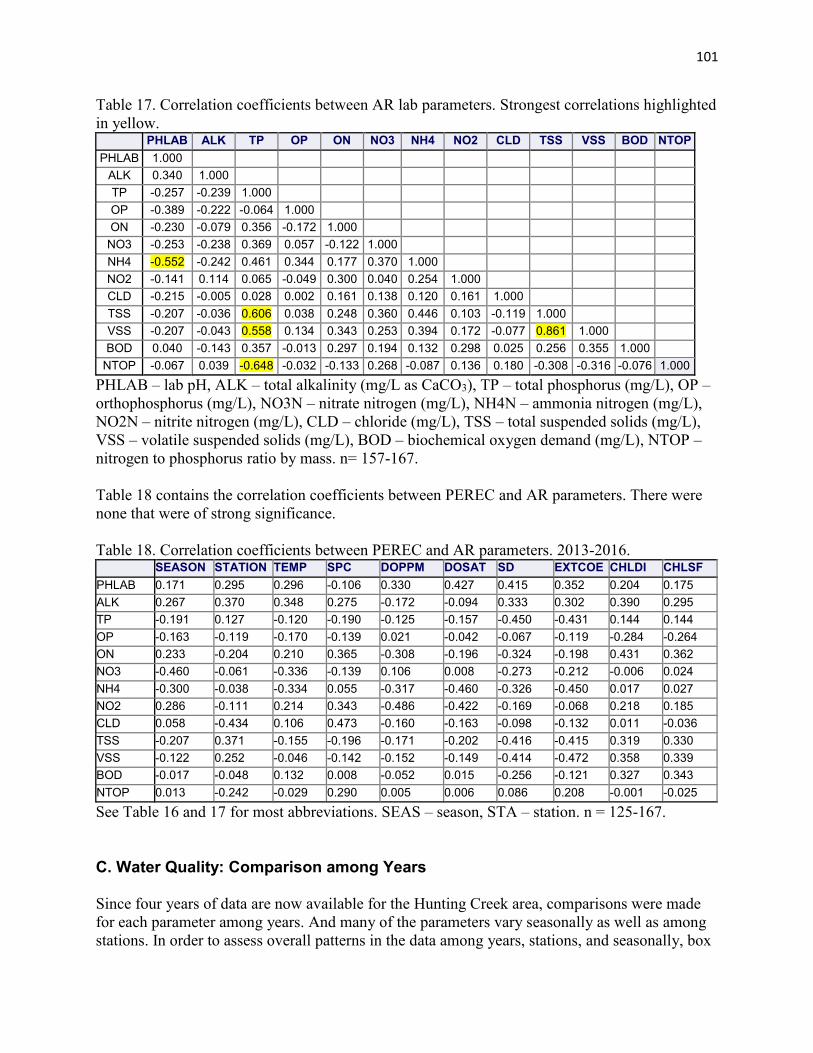
101

Table 17. Correlation coefficients between AR lab parameters. Strongest correlations highlighted in yellow.

PHLAB ALK TP OP ON NO3 NH4 NO2 CLD TSS VSS BOD NTOP PHLAB 1.000

ALK 0.340 1.000

TP -0.257 -0.239 1.000

OP -0.389 -0.222 -0.064 1.000

ON -0.230 -0.079 0.356 -0.172 1.000

NO3 -0.253 -0.238 0.369 0.057 -0.122 1.000

NH4 -0.552 -0.242 0.461 0.344 0.177 0.370 1.000

NO2 -0.141 0.114 0.065 -0.049 0.300 0.040 0.254 1.000

CLD -0.215 -0.005 0.028 0.002 0.161 0.138 0.120 0.161 1.000

TSS -0.207 -0.036 0.606 0.038 0.248 0.360 0.446 0.103 -0.119 1.000

VSS -0.207 -0.043 0.558 0.134 0.343 0.253 0.394 0.172 -0.077 0.861 1.000

BOD 0.040 -0.143 0.357 -0.013 0.297 0.194 0.132 0.298 0.025 0.256 0.355 1.000

NTOP -0.067 0.039 -0.648 -0.032 -0.133 0.268 -0.087 0.136 0.180 -0.308 -0.316 -0.076 1.000

PHLAB – lab pH, ALK – total alkalinity (mg/L as CaCO3), TP – total phosphorus (mg/L), OP – orthophosphorus (mg/L), NO3N – nitrate nitrogen (mg/L), NH4N – ammonia nitrogen (mg/L), NO2N – nitrite nitrogen (mg/L), CLD – chloride (mg/L), TSS – total suspended solids (mg/L), VSS – volatile suspended solids (mg/L), BOD – biochemical oxygen demand (mg/L), NTOP – nitrogen to phosphorus ratio by mass. n= 157-167. Table 18 contains the correlation coefficients between PEREC and AR parameters. There were none that were of strong significance. Table 18. Correlation coefficients between PEREC and AR parameters. 2013-2016. SEASON STATION TEMP SPC DOPPM DOSAT SD EXTCOE CHLDI CHLSF PHLAB 0.171 0.295 0.296 -0.106 0.330 0.427 0.415 0.352 0.204 0.175 ALK 0.267 0.370 0.348 0.275 -0.172 -0.094 0.333 0.302 0.390 0.295 TP -0.191 0.127 -0.120 -0.190 -0.125 -0.157 -0.450 -0.431 0.144 0.144 OP -0.163 -0.119 -0.170 -0.139 0.021 -0.042 -0.067 -0.119 -0.284 -0.264 ON 0.233 -0.204 0.210 0.365 -0.308 -0.196 -0.324 -0.198 0.431 0.362 NO3 -0.460 -0.061 -0.336 -0.139 0.106 0.008 -0.273 -0.212 -0.006 0.024 NH4 -0.300 -0.038 -0.334 0.055 -0.317 -0.460 -0.326 -0.450 0.017 0.027 NO2 0.286 -0.111 0.214 0.343 -0.486 -0.422 -0.169 -0.068 0.218 0.185 CLD 0.058 -0.434 0.106 0.473 -0.160 -0.163 -0.098 -0.132 0.011 -0.036 TSS -0.207 0.371 -0.155 -0.196 -0.171 -0.202 -0.416 -0.415 0.319 0.330 VSS -0.122 0.252 -0.046 -0.142 -0.152 -0.149 -0.414 -0.472 0.358 0.339 BOD -0.017 -0.048 0.132 0.008 -0.052 0.015 -0.256 -0.121 0.327 0.343 NTOP 0.013 -0.242 -0.029 0.290 0.005 0.006 0.086 0.208 -0.001 -0.025

See Table 16 and 17 for most abbreviations. SEAS – season, STA – station. n = 125-167. C. Water Quality: Comparison among Years Since four years of data are now available for the Hunting Creek area, comparisons were made for each parameter among years. And many of the parameters vary seasonally as well as among stations. In order to assess overall patterns in the data among years, stations, and seasonally, box

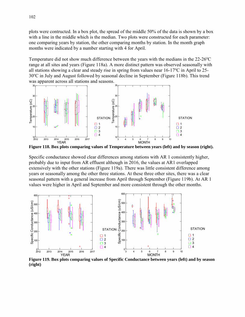
102

plots were contructed. In a box plot, the spread of the middle 50% of the data is shown by a box with a line in the middle which is the median. Two plots were constructed for each parameter: one comparing years by station, the other comparing months by station. In the month graph months were indicated by a number starting with 4 for April. Temperature did not show much difference between the years with the medians in the 22-26oC range at all sites and years (Figure 118a). A more distinct pattern was observed seasonally with all stations showing a clear and steady rise in spring from values near 16-17oC in April to 25-30oC in July and August followed by seasonal decline in September (Figure 118b). This trend was apparent across all stations and seasons.

Figure 118. Box plots comparing values of Temperature between years (left) and by season (right).

Specific conductance showed clear differences among stations with AR 1 consistently higher, probably due to input from AR effluent although in 2016, the values at AR1 overlapped extensively with the other stations (Figure 119a). There was little consistent difference among years or seasonally among the other three stations. At these three other sites, there was a clear seasonal pattern with a general increase from April through September (Figure 119b). At AR 1 values were higher in April and September and more consistent through the other months.

Figure 119. Box plots comparing values of Specific Conductance between years (left) and by season

(right)

4321

STATION

2012 2013 2014 2015 2016 2017YEAR

10

15

20

25

30

35

Tem

pera

ture

(oC

)

4321

STATION

3 4 5 6 7 8 9 10MONTH

10

15

20

25

30

35

Tem

pera

ture

(oC

)

4321

STATION

2012 2013 2014 2015 2016 2017YEAR

0

100

200

300

400

500

600

Spe

cific

Con

duct

ance

(uS

/cm

)

4321

STATION

3 4 5 6 7 8 9 10MONTH

0

100

200

300

400

500

600

Spe

cific

Con

duct

ance

(uS

/cm

)

103

Figure 120. Box plots comparing values of dissolved oxygen as mg/L between years (left) and by

season (right).

Median dissolved oxygen (mg/L) values exhibited more outliers in 2016 than in most other years (Figure 120a). These were mostly at AR2. The high outliers were associated with strong SAV photosynthesis. There was one low outlier that was below the DO standard of 5 mg/L. Values were generally highest in April, except at AR2 and AR3 where July and August exhibited some higher values (Figure 120b). Dissolved oxygen (as % saturation) did not vary much between years at AR4 (Figure 121a). At AR2 and AR3 there was a greater range of values in several years in the months of July and August (Figure 121b). These are the months of high SAV abundance.

Figure 121. Box plots comparing values of dissolved oxygen as percent saturation between years

(left) and by season (right).

4321

STATION

2012 2013 2014 2015 2016 2017YEAR

0

5

10

15

20D

isso

lved

oxy

gen

(mg/

L)

4321

STATION

3 4 5 6 7 8 9 10MONTH

0

5

10

15

20

Dis

solv

ed o

xyge

n (m

g/L)

4321

STATION

2012 2013 2014 2015 2016 2017YEAR

0

50

100

150

200

Dis

solv

ed o

xyge

n (%

sat

urat

ion)

4321

STATION

3 4 5 6 7 8 9 10MONTH

0

50

100

150

200

Dis

solv

ed o

xyge

n (%

sat

urat

ion)

104

Figure 122. Box plots comparing values of field pH between years (left) and by season (right).

Field pH was consistently lowest at AR1 though still in a healthy range (Figure 122a). Generally AR3 was the highest and AR2 was second highest and the elevated values at these sites was most obvious in July and August (Figure 122b), periods of high SAV abundance. Secchi disk depth (Figure 123a) did not show any obvious interannual patterns among stations or seasonally. There are many missing values at AR2 and AR3 in the summer and fall due to the encroachment of SAV into the watercolumn and the shallow dept of these areas (Figure 123b). Secchi disk measurements were discontinued at AR1 when a new sampling protocol was instituted there.

Figure 123. Box plots comparing values of Secchi disk depth between years (left) and by season

(right).

4321

STATION

2012 2013 2014 2015 2016 2017YEAR

6

7

8

9

10Fi

eld

pH

4321

STATION

3 4 5 6 7 8 9 10MONTH

6

7

8

9

10

Fiel

d pH

4321

STATION

2012 2013 2014 2015 2016 2017YEAR

0.0

0.5

1.0

1.5

2.0

Sec

chi D

isk

Dep

th (m

)

4321

STATION

3 4 5 6 7 8 9 10MONTH

0.0

0.5

1.0

1.5

2.0

Sec

chi D

isk

Dep

th (m

)

105

Figure 124. Box plots comparing values of Light Attenuation Coefficient between years (left) and by

season (right).

Light attenuation coefficient and turbidity are two other ways of measuring water clarity: higher values of light attenution coefficient indicate clearer water. Median values in light attenuation coefficient were similar from year to year (Figure 124a). There was little consistent seasonal pattern (Figure 124b). Turbidity, another measure of water clarity, increased at AR4 from 2013 to 2014 and 2015, but declined a bit in 2016 (Figure 125a). At the other stations, interannual trends in median values was not apparent, but their was great variability within a year in 2015. When viewed seasonally, AR4 tended to show increasing values from April through September (Figure 125b). Values at AR2 and AR3 increased slightly from April through June and then declined in July and August similar to trends in light attenuation coefficient. AR1 also declined through the year.

Figure 125. Box plots comparing values of Turbidity between years (left) and by season (right).

4321

STATION

2012 2013 2014 2015 2016 2017YEAR

-7

-6

-5

-4

-3

-2

-1

0

Ligh

t Atte

nuat

ion

Coe

ffici

ent (

m-1

)

4321

STATION

3 4 5 6 7 8 9 10MONTH

-7

-6

-5

-4

-3

-2

-1

0

Ligh

t Atte

nuat

ion

Coe

ffici

ent (

m-1

)

4321

STATION

2012 2013 2014 2015 2016 2017YEAR

1

10

100

Turb

idity

, YS

I

4321

STATION

3 4 5 6 7 8 9 10MONTH

1

10

100

Turb

idity

, YS

I

106

Figure 126. Box plots comparing values of Total Phosphorus between years (left) and by season

(right).

Total phosphorus did not exhibit any clear patterns between years (Figure 126a). Seasonally, there was a steady decline in Total P from spring through fall in the embayment stations (AR1, AR2, and AR3) while the river station (AR4) did not show much seasonal trend (Figure 126b). Organic nitrogen was generally higher at AR1 than at the other stations (Figure 127a). This effect was most pronounced in spring when there was a pattern of decreasing values from AR1 to AR2 to AR3 to AR4 (Figure 127b). This pattern started breaking down in July and disappered in August and September.

Figure 127. Box plots comparing values of Organic Nitrogen between years (left) and by season

(right).

4321

STATION

2012 2013 2014 2015 2016 2017YEAR

0.0

0.1

0.2

0.3To

tal P

hosp

horu

s (m

g/L)

4321

STATION

3 4 5 6 7 8 9 10MONTH

0.0

0.1

0.2

0.3

Tota

l Pho

spho

rus

(mg/

L)

4321

STATION

2012 2013 2014 2015 2016 2017YEAR

0.1

1.0

Org

anic

Nitr

ogen

(mg/

L)

4321

STATION

3 4 5 6 7 8 9 10MONTH

0.1

1.0

Org

anic

Nitr

ogen

(mg/

L)

107

Figure 128. Box plots comparing values of Nitrate Nitrogen between years (left) and by season

(right).

Nitrate nitrogen values continued to be substantially lower than in the first two years of the study (Figure 128a). A seasonal pattern in nitrate values was observed with a decline at all stations in summer attributable to uptake by phytoplankton and SAV (Figure 128b). Ammonia nitrogen values did not show any systematic variation among the years (Figure 129a). A seasonal pattern, however was apparent with values in the period July to September being substantially lower than observed in the previous months (Figure 129b).

Figure 129. Box plots comparing values of Ammonia Nitrogen between years (left) and by season

(right).

4321

STATION

2012 2013 2014 2015 2016 2017YEAR

0.1

1.0

Nitr

ate

Nitr

ogen

(mg/

L)

4321

STATION

3 4 5 6 7 8 9 10MONTH

0.1

1.0

Nitr

ate

Nitr

ogen

(mg/

L)

4321

STATION

2012 2013 2014 2015 2016 2017YEAR

0.01

0.10

1.00

Am

mon

ia N

itrog

en (m

g/L)

4321

STATION

3 4 5 6 7 8 9 10MONTH

0.01

0.10

1.00

Am

mon

ia N

itrog

en (m

g/L)

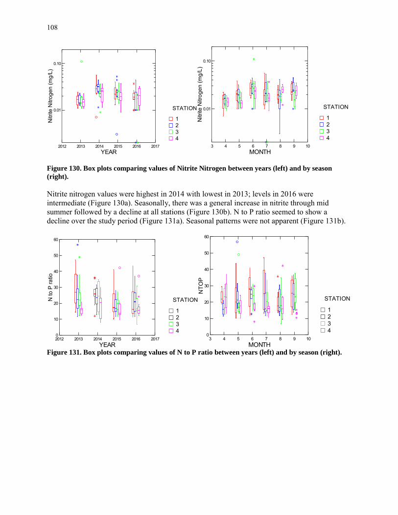
108

Figure 130. Box plots comparing values of Nitrite Nitrogen between years (left) and by season

(right).

Nitrite nitrogen values were highest in 2014 with lowest in 2013; levels in 2016 were intermediate (Figure 130a). Seasonally, there was a general increase in nitrite through mid summer followed by a decline at all stations (Figure 130b). N to P ratio seemed to show a decline over the study period (Figure 131a). Seasonal patterns were not apparent (Figure 131b).

Figure 131. Box plots comparing values of N to P ratio between years (left) and by season (right).

4321

STATION

2012 2013 2014 2015 2016 2017YEAR

0.01

0.10

Nitr

ite N

itrog

en (m

g/L)

4321

STATION

3 4 5 6 7 8 9 10MONTH

0.01

0.10

Nitr

ite N

itrog

en (m

g/L)

4321

STATION

2012 2013 2014 2015 2016 2017YEAR

0

10

20

30

40

50

60

N to

P ra

tio

4321

STATION

3 4 5 6 7 8 9 10MONTH

0

10

20

30

40

50

60

NTO

P

109

Figure 132. Box plots comparing values of Total Suspended Solids between years (left) and by

season (right).

Total suspended solids (TSS) have not shown any clear trends over the four years of the study (Figure 132a). Seasonal patterns were different between the river mainstem site (AR4) and the Hunting Creek embayment stations (AR1, AR2, AR3). At AR4 TSS tended to rise through the study period whereas at the other sites it showed a marked decline particulary when the SAV beds were highly developed in August and September (Figure 132b). VSS exhibited little systematic variation among years, but a seasonal pattern similar to that of TSS (Figure 133a,b).

Figure 133. Box plots comparing values of Volitile Suspended Solids between years (left) and by

season (right).

4321

STATION

2012 2013 2014 2015 2016 2017YEAR

1

10

100

Tota

l Sus

pend

ed S

olid

s (m

g/L)

4321

STATION

3 4 5 6 7 8 9 10MONTH

1

10

100

Tota

l Sus

pend

ed S

olid

s (m

g/L)

4321

STATION

2012 2013 2014 2015 2016 2017YEAR

1

10

Vol

atile

Sus

pend

ed S

olid

s (m

g/L)

4321

STATION

3 4 5 6 7 8 9 10MONTH

1

10

VS

S

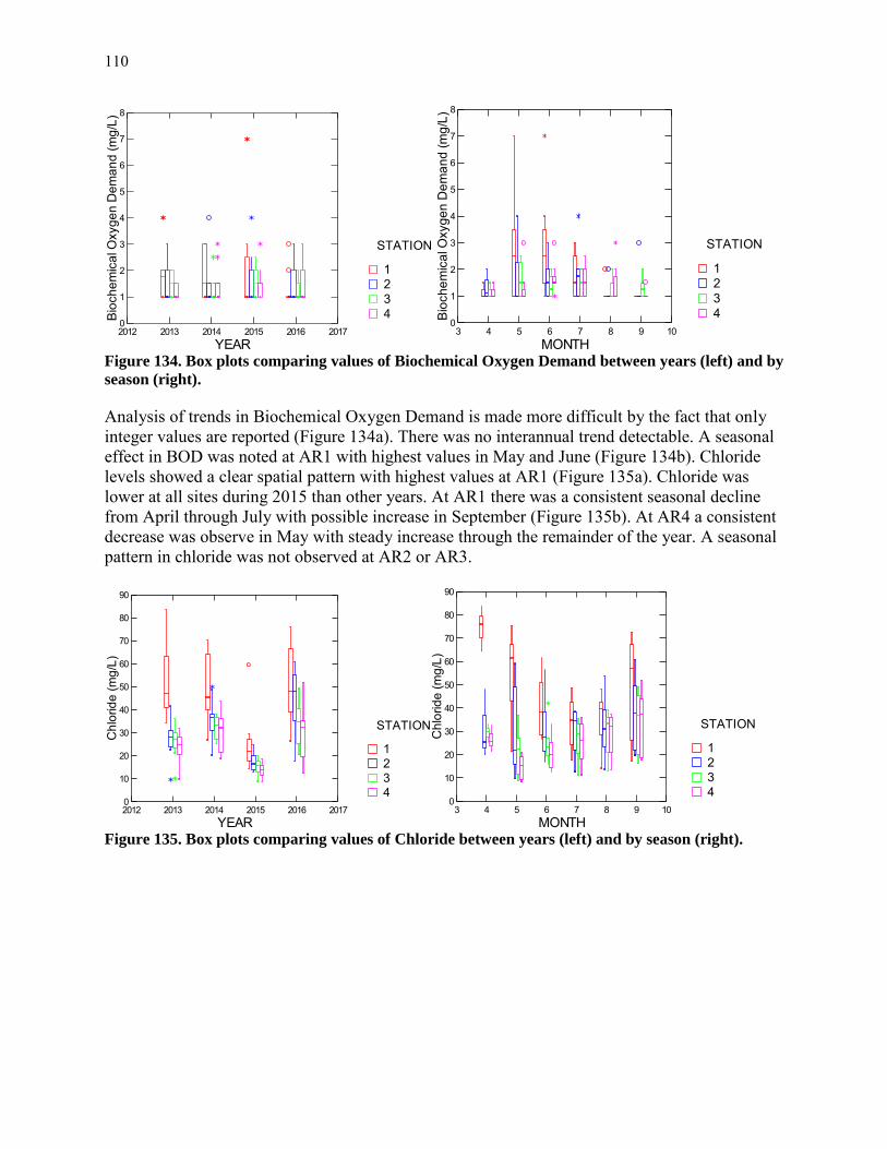
110

Figure 134. Box plots comparing values of Biochemical Oxygen Demand between years (left) and by

season (right).

Analysis of trends in Biochemical Oxygen Demand is made more difficult by the fact that only integer values are reported (Figure 134a). There was no interannual trend detectable. A seasonal effect in BOD was noted at AR1 with highest values in May and June (Figure 134b). Chloride levels showed a clear spatial pattern with highest values at AR1 (Figure 135a). Chloride was lower at all sites during 2015 than other years. At AR1 there was a consistent seasonal decline from April through July with possible increase in September (Figure 135b). At AR4 a consistent decrease was observe in May with steady increase through the remainder of the year. A seasonal pattern in chloride was not observed at AR2 or AR3.

Figure 135. Box plots comparing values of Chloride between years (left) and by season (right).

4321

STATION

2012 2013 2014 2015 2016 2017YEAR

0

1

2

3

4

5

6

7

8B

ioch

emic

al O

xyge

n D

eman

d (m

g/L)

4321

STATION

3 4 5 6 7 8 9 10MONTH

0

1

2

3

4

5

6

7

8

Bio

chem

ical

Oxy

gen

Dem

and

(mg/

L)

4321

STATION

2012 2013 2014 2015 2016 2017YEAR

0

10

20

30

40

50

60

70

80

90

Chl

orid

e (m

g/L)

4321

STATION

3 4 5 6 7 8 9 10MONTH

0

10

20

30

40

50

60

70

80

90

Chl

orid

e (m

g/L)

111

Figure 136. Box plots comparing values of Total Alkalinity between years (left) and by season

(right).

Total alkalinity showed little difference among the years but within each year there was a clear pattern among each year by station: AR1 being lowest and AR4 being highest (Figure 136a). There was a suggestion of decline in alkalinity in May followed by an increase through the rest of the year at most sites (Figure 136b).

4321

STATION

2012 2013 2014 2015 2016 2017YEAR

0

20

40

60

80

100

120To

tal A

lkal

inity

(mg/

L as

CaC

O3)

4321

STATION

3 4 5 6 7 8 9 10MONTH

0

20

40

60

80

100

120

Tota

l Alk

allin

ity (m

g/L

as C

aCO

3)

112

D. Phytoplankton: Comparison among Years

Figure 137. Box plots comparing values of depth-integrated Chlorophyll a among years (left) and

by month (right).

A general decline in depth-integrated chlorophyll was observed at AR2 and AR3 over the study period (Figure 137a). A seasonal increase with maximum in July and August was clearly indicated at AR4, whereas AR2 and AR3 did not show a consistent seasonal effect (Figure 137b). Similar results were observed with surface chlorophyll (Figure 138a,b). Chlorophyll values in the water are a measure of phytoplankton populations which compete with phytoplankton for light and nutrients.

Figure 98. Box plots comparing values of surface Chlorophyll a among years (left) and by month

(right).

4321

STATION

2012 2013 2014 2015 2016 2017YEAR

1

10

Chl

orop

hyll

a, D

I (ug

/L)

4321

STATION

3 4 5 6 7 8 9 10MONTH

1

10

Chl

orop

hyll

a, D

I (ug

/L)

4321

STATION

2012 2013 2014 2015 2016 2017YEAR

1

10

Chl

orop

hyll

a, S

urfa

ce (u

g/L)

4321

STATION

3 4 5 6 7 8 9 10MONTH

1

10

Chl

orop

hyll

a, S

urfa

ce (u

g/L)

113

Figure 139. Box plots comparing values of Total Phytoplankton Density among years (left) and by

month (right).

The median values for total phytoplankton cell density were similar among the three years, although there were more high values in 2014 (Figure 139a). Both stations showed a seasonal increase in phytoplankton (Figure 139b). The increase followed a similar pattern at both stations through July, but in August AR4 (river mainstem) continued to increase whereas at AR2 (Hunting Creek) values leveled off. Total cyanobacterial cell density was clearly higher in 2014 at both stations than in the other three years (Figure 140a). The main difference between the two stations was the greater variability observed at AR4. The seasonal pattern in cyanobacterial density was very similar to the patterns noted above in total phytoplankton cell density as cyanobacteria often make up the majority of phytoplankton cells (Figure 140b).

Figure 140. Box plots comparing values of Cyanobacterial Density among years (left) and by month

(right).

42

SITE

2012 2013 2014 2015 2016 2017YEAR

10000

100000

1000000To

tal P

hyto

plan

kton

Den

sity

(#/m

L)

42

SITE

3 4 5 6 7 8 9 10MONTH

10000

100000

1000000

Tota

l Phy

topl

ankt

on D

ensi

ty (#

/mL)

42

SITE

2012 2013 2014 2015 2016 2017YEAR

10000

100000

1000000

Tota

l Cya

noba

cter

ia D

ensi

ty (#

/mL)

42

SITE

3 4 5 6 7 8 9 10MONTH

10000

100000

1000000

Tota

l Cya

noba

cter

ia D

ensi

ty (#

/mL)

114

Figure 141. Box plots comparing values of Diatom Density among years (left) and by month (right).

Median diatom densities overall were fairly constant among all years at AR4 (Figure 141a). At AR2, lower medians were found in 2014 and 2015 relative to 2013; 2016 values were intermediate. Median diatom densities were highest in April at AR2, lowest in May, June and July (Figure 141b). At AR4 a decline was observed in May and then values increased through August. Green algal cell densities were very similar across the three years (Figure 142a). A seasonal pattern of spring increase and summer decline was suggested at AR4 (Figure 142b). At AR2 a similar pattern was observed except that September exhibited an increase.

Figure 142. Box plots comparing values of Green Algal Density among years (left) and by month

(right).

42

SITE

2012 2013 2014 2015 2016 2017YEAR

1000

10000

100000

Tota

l Dia

tom

Den

sity

(#/m

L)

42

SITE

3 4 5 6 7 8 9 10MONTH

1000

10000

100000

Tota

l Dia

tom

Den

sity

(#/m

L)

42

SITE

2012 2013 2014 2015 2016 2017YEAR

1000

10000

100000

Tota

l Gre

en A

lgae

Den

sity

(#/m

L)

42

SITE

3 4 5 6 7 8 9 10MONTH

1000

10000

100000

Tota

l Gre

en A

lgae

Den

sity

(#/m

L)

115

Figure 143. Box plots comparing values of Cryptophyte Density among years (left) and by month

(right).

Median cryptophyte cell densities have generally declined over the study period at AR2 (Figure 143a). At AR4 values were lower in 2015, but increased again in 2016.. A general seasonal pattern of higher values in spring and a tapering for the rest of the year was found at both stations (Figure 143b). Miscellaneous taxa includes those species of phytoplankton in groups not tallied above. These are mainly dinoflagellates, crysophytes and euglenoids whose abundances are somewhat sporadic in the study area. This is reflected in interannual and seasonal patterns which did not reveal any clear patterns (Figure 144a,b).

Figure 144. Box plots comparing values of Miscellaneous Taxa Density among years (left) and by

month (right).

42

SITE

2012 2013 2014 2015 2016 2017YEAR

10000

Tota

l Cry

ptop

hyte

Den

sity

(#/m

L)

42

SITE

3 4 5 6 7 8 9 10MONTH

10000

Tota

l Cry

ptop

hyte

Den

sity

(#/m

L)

42

SITE

2012 2013 2014 2015 2016 2017YEAR

1000

10000

Tota

l Mis

c. T

axa

Den

sity

(#/m

L)

42

SITE

3 4 5 6 7 8 9 10MONTH

1000

10000

Tota

l Mis

c. T

axa

Den

sity

(#/m

L)

116

Figure 145. Box plots comparing values of Total Phytoplankton Biovolume among years (left) and

by month (right).

Biovolume takes into account both the number of cells and their relative size. Mean values of total phytoplankton biovolume were similar over all three years at AR2 (Figure 145a). At AR4 total phytoplankton biovolume was markedly higher in 2014 than in the other two years. At AR2 there was little seasonal pattern, but at AR4 a general decline was observed in May and June followed by an increase in July and August (Figure 145b). Total cyanobacterial biovolume exhibited a steady decline in median values through 2015, but values rebounded somewhat at both sites in 2016 (Figure 146a). Seasonally both values at both stations increased through August. AR2 was generally higher in spring and early summer and AR4 was higher in late summer and fall (146b).

Figure 146. Box plots comparing values of Cyanobacterial Biovolume among years (left) and by

month (right).

42

SITE

2012 2013 2014 2015 2016 2017YEAR

10000000

100000000

Tota

l Phy

topl

ankt

on B

iovo

l (um

3/L)

42

SITE

3 4 5 6 7 8 9 10MONTH

10000000

100000000

Tota

l Phy

topl

ankt

on B

iovo

l (um

3/L)

42

SITE

2012 2013 2014 2015 2016 2017YEAR

100000

1000000

10000000

Tota

l Cya

noba

cter

ium

Bio

vol (

um3/

L)

42

SITE

3 4 5 6 7 8 9 10MONTH

100000

1000000

10000000

Tota

l Cya

noba

cter

ium

Bio

vol (

um3/

L)

117

Figure 147. Box plots comparing values of Diatom Biovolume among years (left) and by month

(right).

Median diatom biovolume did not show a consistent trend over the four years of the study (Figure 147a). Median value at AR2 declined steadily over the study period while values at AR4 tended to increased. Seasonal patterns revealed that a general increase was observed at both stations from April through July (Figure 147b). At AR4 the increase continued through August whereas at AR2 the seasonal decline began in August. Median values in green algal biovolume have shown some pattern of increase over the study period (Figure 148a). The seasonal pattern was complex, but similar at both stations (Figure 148b). Increase from April to May was followed by decreases through July and a recovery in September.

Figure 148. Box plots comparing values of Green Algal Biovolume among years (left) and by month

(right).

42

SITE

2012 2013 2014 2015 2016 2017YEAR

1000000

10000000

100000000

Tota

l Dia

tom

Bio

vol (

um3/

L)

42

SITE

3 4 5 6 7 8 9 10MONTH

1000000

10000000

100000000

Tota

l Dia

tom

Bio

vol (

um3/

L)

42

SITE

2012 2013 2014 2015 2016 2017YEAR

100000

1000000

10000000

Tota

l Gre

en A

lgae

Bio

vol (

um3/

L)

42

SITE

3 4 5 6 7 8 9 10MONTH

100000

1000000

10000000

Tota

l Gre

en A

lgae

Bio

vol (

um3/

L)

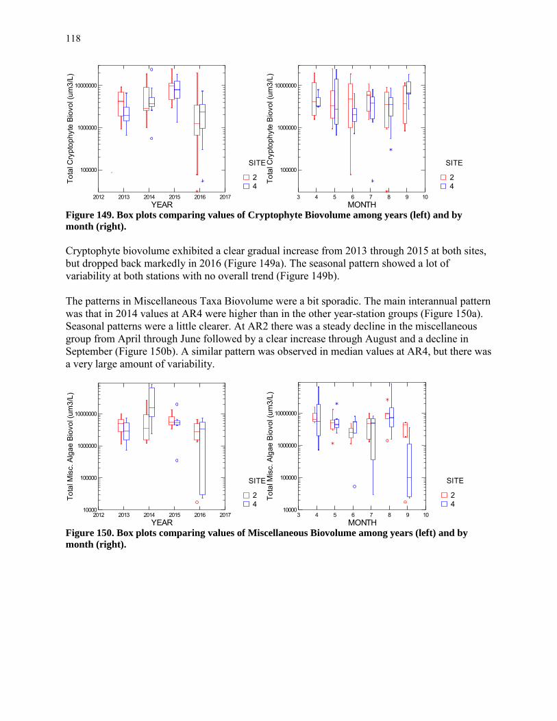
118

Figure 149. Box plots comparing values of Cryptophyte Biovolume among years (left) and by

month (right).

Cryptophyte biovolume exhibited a clear gradual increase from 2013 through 2015 at both sites, but dropped back markedly in 2016 (Figure 149a). The seasonal pattern showed a lot of variability at both stations with no overall trend (Figure 149b). The patterns in Miscellaneous Taxa Biovolume were a bit sporadic. The main interannual pattern was that in 2014 values at AR4 were higher than in the other year-station groups (Figure 150a). Seasonal patterns were a little clearer. At AR2 there was a steady decline in the miscellaneous group from April through June followed by a clear increase through August and a decline in September (Figure 150b). A similar pattern was observed in median values at AR4, but there was a very large amount of variability.

Figure 150. Box plots comparing values of Miscellaneous Biovolume among years (left) and by

month (right).

42

SITE

2012 2013 2014 2015 2016 2017YEAR

100000

1000000

10000000

Tota

l Cry

ptop

hyte

Bio

vol (

um3/

L)

42

SITE

3 4 5 6 7 8 9 10MONTH

100000

1000000

10000000

Tota

l Cry

ptop

hyte

Bio

vol (

um3/

L)

42

SITE

2012 2013 2014 2015 2016 2017YEAR

10000

100000

1000000

10000000

Tota

l Mis

c. A

lgae

Bio

vol (

um3/

L)

42

SITE

3 4 5 6 7 8 9 10MONTH

10000

100000

1000000

10000000

Tota

l Mis

c. A

lgae

Bio

vol (

um3/

L)

119

Figure 151. Box plots comparing values of Melosira Biovolume among years (left) and by month

(right).

An analysis of interannual and seasonal effects also done for selected individual taxa. Median biovolume values of the filamentous diatom Melosira showed a clear peak in 2014 at both stations (Figure 151a). Melosira also exhibited a clear seasonal pattern of increase from April through July at AR2 (Figure 151b). At AR4 April was highest. Discoid centric biovolume was also highest in 2014 at AR4 (Figure 152a). At AR2 the year of highest median biovolume was 2013. Seasonal patterns generally indicated that values were relatively high at AR2 in the sping but declined through August (Figure 152b). At AR4 discoid centrics were less abundant in the spring and increased reaching a peak in mid to late summer.

Figure 152. Box plots comparing values of Discoid Centric Diatom Biovolume among years (left)

and by month (right).

42

SITE

2012 2013 2014 2015 2016 2017YEAR

1000000

10000000

100000000

Mel

osira

Bio

lvol

(um

3/m

L)

42

SITE

3 4 5 6 7 8 9 10MONTH

1000000

10000000

100000000

Mel

osira

Bio

lvol

(um

3/m

L)

42

SITE

2012 2013 2014 2015 2016 2017YEAR

100000

1000000

10000000

Dis

coid

cen

tric

Bio

lvol

(um

3/m

L)

42

SITE

3 4 5 6 7 8 9 10MONTH

100000

1000000

10000000

Dis

coid

cen

tric

Bio

lvol

(um

3/m

L)

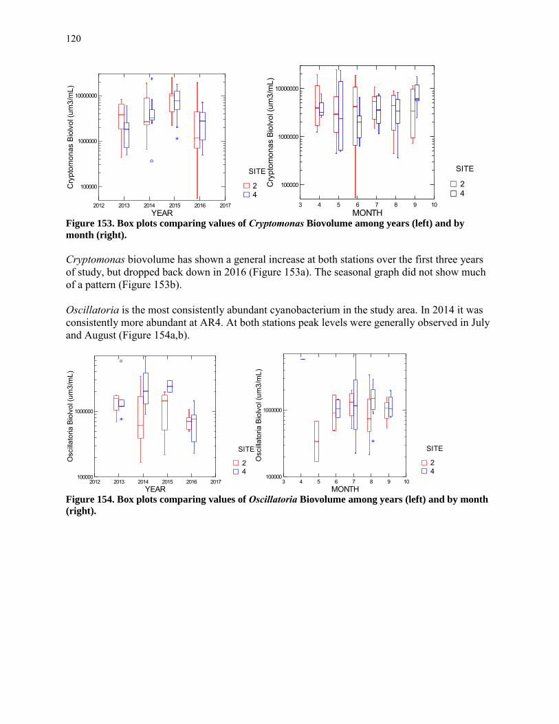
120

Figure 153. Box plots comparing values of Cryptomonas Biovolume among years (left) and by

month (right).

Cryptomonas biovolume has shown a general increase at both stations over the first three years of study, but dropped back down in 2016 (Figure 153a). The seasonal graph did not show much of a pattern (Figure 153b). Oscillatoria is the most consistently abundant cyanobacterium in the study area. In 2014 it was consistently more abundant at AR4. At both stations peak levels were generally observed in July and August (Figure 154a,b).

Figure 154. Box plots comparing values of Oscillatoria Biovolume among years (left) and by month

(right).

42

SITE

2012 2013 2014 2015 2016 2017YEAR

100000

1000000

10000000

Cry

ptom

onas

Bio

lvol

(um

3/m

L)

42

SITE

3 4 5 6 7 8 9 10MONTH

100000

1000000

10000000

Cry

ptom

onas

Bio

lvol

(um

3/m

L)

42

SITE

2012 2013 2014 2015 2016 2017YEAR

100000

1000000

Osc

illato

ria B

iolv

ol (u

m3/

mL)

42

SITE

3 4 5 6 7 8 9 10MONTH

100000

1000000

Osc

illato

ria B

iolv

ol (u

m3/

mL)

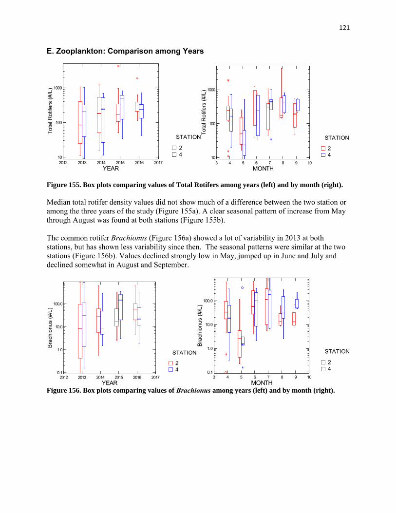
121

E. Zooplankton: Comparison among Years

Figure 155. Box plots comparing values of Total Rotifers among years (left) and by month (right).

Median total rotifer density values did not show much of a difference between the two station or among the three years of the study (Figure 155a). A clear seasonal pattern of increase from May through August was found at both stations (Figure 155b). The common rotifer Brachionus (Figure 156a) showed a lot of variability in 2013 at both stations, but has shown less variability since then. The seasonal patterns were similar at the two stations (Figure 156b). Values declined strongly low in May, jumped up in June and July and declined somewhat in August and September.

Figure 156. Box plots comparing values of Brachionus among years (left) and by month (right).

42

STATION

2012 2013 2014 2015 2016 2017YEAR

10

100

1000

Tota

l Rot

ifers

(#/L

)

42

STATION

3 4 5 6 7 8 9 10MONTH

10

100

1000

Tota

l Rot

ifers

(#/L

)

42

STATION

2012 2013 2014 2015 2016 2017YEAR

0.1

1.0

10.0

100.0

Bra

chio

nus

(#/L

)

42

STATION

3 4 5 6 7 8 9 10MONTH

0.1

1.0

10.0

100.0

Bra

chio

nus

(#/L

)

122

Figure 157. Box plots comparing values of Keratella among years (left) and by month (right).

Another common rotifer Keratella was clearly more abundant at AR4 than AR2 in all years (Figure 157a). The seasonal pattern was one of fairly consistent increase from spring through late summer at both stations (Figure 157b). Polyarthra was variable and generally present at lower levels than Brachionus or Keratella. Few Polyarthra were observed at AR4 in 2014, but otherwise there was little difference among years (Figure 158a). Seasonal patterns were variable, but spring values were consistently lower than densities observed later in the year (Figure 158b).

Figure 158. Box plots comparing values of Polyarthra among years (left) and by month (right).

42

STATION

2012 2013 2014 2015 2016 2017YEAR

10

100

Ker

atel

la (#

/L)

42

STATION

3 4 5 6 7 8 9 10MONTH

10

100

Ker

atel

la (#

/L)

42

STATION

2012 2013 2014 2015 2016 2017YEAR

0.1

1.0

10.0

Pol

yarth

ra (#

/L)

42

STATION

3 4 5 6 7 8 9 10MONTH

0.1

1.0

10.0

Pol

yarth

ra (#

/L)

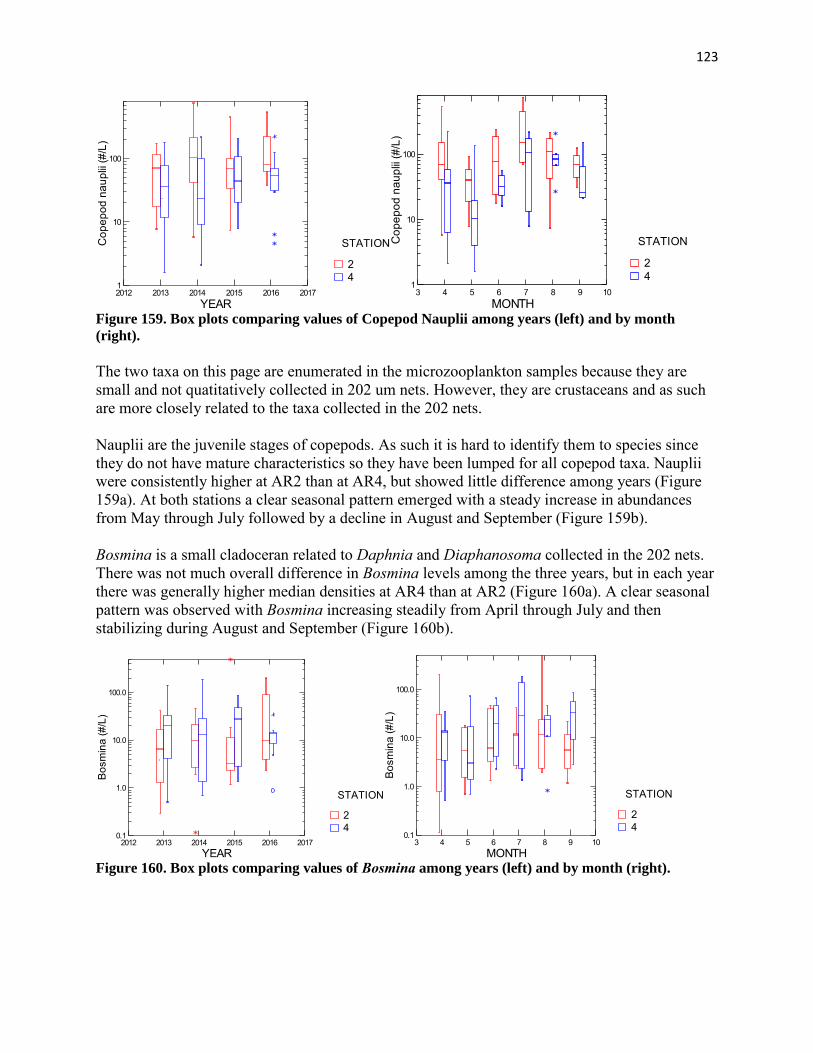
123

Figure 159. Box plots comparing values of Copepod Nauplii among years (left) and by month

(right).

The two taxa on this page are enumerated in the microzooplankton samples because they are small and not quatitatively collected in 202 um nets. However, they are crustaceans and as such are more closely related to the taxa collected in the 202 nets. Nauplii are the juvenile stages of copepods. As such it is hard to identify them to species since they do not have mature characteristics so they have been lumped for all copepod taxa. Nauplii were consistently higher at AR2 than at AR4, but showed little difference among years (Figure 159a). At both stations a clear seasonal pattern emerged with a steady increase in abundances from May through July followed by a decline in August and September (Figure 159b). Bosmina is a small cladoceran related to Daphnia and Diaphanosoma collected in the 202 nets. There was not much overall difference in Bosmina levels among the three years, but in each year there was generally higher median densities at AR4 than at AR2 (Figure 160a). A clear seasonal pattern was observed with Bosmina increasing steadily from April through July and then stabilizing during August and September (Figure 160b).

Figure 160. Box plots comparing values of Bosmina among years (left) and by month (right).

42

STATION

2012 2013 2014 2015 2016 2017YEAR

1

10

100

Cop

epod

nau

plii

(#/L

)

42

STATION

3 4 5 6 7 8 9 10MONTH

1

10

100

Cop

epod

nau

plii

(#/L

)

42

STATION

2012 2013 2014 2015 2016 2017YEAR

0.1

1.0

10.0

100.0

Bos

min

a (#

/L)

42

STATION

3 4 5 6 7 8 9 10MONTH

0.1

1.0

10.0

100.0

Bos

min

a (#

/L)

124

Figure 161. Box plots comparing values of Total Calanoid Copepods among years (left) and by

month (right).

Median calanoid copepod densities were similar among the years at AR4 (Figure 161a).

At AR4 values were generally lower than at AR2 and were much lower in 2015. Seasonal patterns indicated that AR2 peaked in the April and May and then delcined through September (Figure 161b). Levels at AR4 were gerally highest in June.

Eurytemora is the most common calanoid copepod. Its interannual pattern was quite similar to that observed for total calanoids (Figure 162a) with AR4 clearly higher than AR2 in 2013, 2015, and 2016. Seasonally, it was more abundant at AR2 in April and May and more abundant at AR4 for the remainder of the year (Figure 162b). Highest densities were observed in June at AR4.

Figure 162. Box plots comparing values of Eurytemora among years (left) and by month (right).

42

STATION

2012 2013 2014 2015 2016 2017YEAR

1

10

100

1000

10000

Tota

l Cal

anoi

d C

opep

ods

(#/m

3)

42

STATION

3 4 5 6 7 8 9 10MONTH

1

10

100

1000

10000

Tota

l Cal

anoi

d C

opep

ods

(#/m

3)

42

STATION

2012 2013 2014 2015 2016 2017YEAR

0.1

1.0

10.0

100.0

1000.0

10000.0

Eur

ytem

ora

(#/m

3)

42

STATION

3 4 5 6 7 8 9 10MONTH

0.1

1.0

10.0

100.0

1000.0

10000.0

Eur

ytem

ora

(#/m

3)

125

Figure 163. Box plots comparing values of Cyclopoid Copepods among years (left) and by month

(right).

Cyclopoid copepods were clearly more abundant in 2014 than in either 2013, 2015 or 2016 at both stations (Figure 163a). Seasonally, levels peaked in June at AR4 and in August at AR2 (Figure 163b).

Mesocyclops is one of the more common cyclopoid copepods. Median values of Mesocyclops was lower at AR2 than in previous years, but at AR 4 they were clearly lower in 2014 (Figure 164a). Seasonal patterns in Mesocyclops were variable (Figure 164b). The most obvious difference was that AR4 was greater than AR2 in June, they both declined strongly in July, and AR2 was greater than AR4 in August.

Figure 164. Box plots comparing values of Mesocyclops among years (left) and by month (right).

42

STATION

2012 2013 2014 2015 2016 2017YEAR

1

10

100

1000

10000

Tota

l Cyc

lopo

id C

opep

ods

(#/m

3)

42

STATION

3 4 5 6 7 8 9 10MONTH

1

10

100

1000

10000

Tota

l Cyc

lopo

id C

opep

ods

(#/m

3)

42

STATION

2012 2013 2014 2015 2016 2017YEAR

1

10

100

1000

Mes

ocyc

lops

(#/m

3)

42

STATION

3 4 5 6 7 8 9 10MONTH

1

10

100

1000

Mes

ocyc

lops

(#/m

3)

126

Figure 165. Box plots comparing values of Total Cladocerans among years (left) and by month

(right).

Total cladoceran values (excluding Bosmina) were clearly lower in 2015 than in the previous two years, but rebounded in 2016 (Figure 165a). A general seasonal pattern was observed with highest values in June (Figure 165b). Values declined quickly in August at AR4, but levels persisted into August at AR2.

Daphnia was found at clearly higher levels in 2014 than in the other three years (Figure 166a). AR2 was clearly greater than AR4 in 2013, but not in the other years. Seasonal patterns consisted of a tendency to higher values in May and Jun than other months (Figure 166b).

Figure 166. Box plots comparing values of Daphnia among years (left) and by month (right).

42

STATION

2012 2013 2014 2015 2016 2017YEAR

10

100

1000

10000To

tal C

lado

cera

ns (#

/m3)

42

STATION

3 4 5 6 7 8 9 10MONTH

10

100

1000

10000

Tota

l Cla

doce

rans

(#/m

3)

42

STATION

2012 2013 2014 2015 2016 2017YEAR

1

10

100

1000

Dap

hnia

(#/m

3)

42

STATION

3 4 5 6 7 8 9 10MONTH

1

10

100

1000

Dap

hnia

(#/m

3)

127

Figure 167. Box plots comparing values of Diaphanosoma among years (left) and by month (right).

Diaphanosoma is a very abundant cladoceran in Gunston Cove, but has proven to be less abundant in the Hunting Creek area, although still important. Diaphanosoma levels were clearly lower in 2015 than in the preceding two years, but rebounded some in 2016 (Figure 167a). Seasonal patterns at both stations indicated increasing populations from April to June followed by a steady decline through September (Figure 167b).

Leptodora is a large predacious cladoceran which occurs consistently in the study area, but at lower densities. Distinct differences were found between years (Figure 168a). AR4 values were similar in 2013 and 2014, but distinctly lower in 2015. At AR2 values were highest in 2013. Leptodora was found principally in the months May, June and July at both stations (Figure 168b).

Figure 168. Box plots comparing values of Leptodora among years (left) and by month (right).

42

STATION

2012 2013 2014 2015 2016 2017YEAR

1

10

100

1000

Dia

phan

osom

a (#

/m3)

42

STATION

3 4 5 6 7 8 9 10MONTH

1

10

100

1000

Dia

phan

osom

a (#

/m3)

42

STATION

2012 2013 2014 2015 2016 2017YEAR

1

10

100

Lept

odor

a (#

/m3)

42

STATION

3 4 5 6 7 8 9 10MONTH

1

10

100

Lept

odor

a (#

/m3)

128

Figure 169. Box plots comparing values of Total Macrozooplankton among years (left) and by

month (right).

Total macrozooplankton, those collected in the 202 um net, showed a clear interannual pattern with greater numbers at both stations in 2014 (Figure a). Seasonal patterns were variable (Figure 169b). At AR4 a spring increased ended with a peak in June. Then values declined throughout the summer. The seasonal pattern was variable at AR2.

42

STATION

2012 2013 2014 2015 2016 2017YEAR

10

100

1000

10000

Tota

l Mac

rozo

opla

nkto

n (#

/m3)

42

STATION

3 4 5 6 7 8 9 10MONTH

10

100

1000

10000

Tota

l Mac

rozo

opla

nkto

n (#

/m3)

129

F. Ichthyoplankton: Comparison among Years 2016 marks the fourth year of our fish collections in Hunting Creek. Both trends and inter-annual variability become apparent when comparing the four years of data. In the larval data a high dominance of different species in the herring or shad family (clupeids) are consistently present, and in high densities (Table 19). These include anadromous species of concern such as blueback herring and alewife, whose spawning populations are monitored for this effort as well. Overall, larval density was lower in 2016 than in previous years. Table 19. Density of larvae collected during 2013-2016.

Species 2013 2014 2015 2016

Alosa aestivalis 61.69 200.35 382.45 91.54 Alosa mediocris 4.80 4.13 12.11 9.63 Alosa pseudoharengus 139.80 57.71 270.62 78.52 Alosa sapidissima 0.12 1.32 0.61 1.97 Alosa sp. 0.00 18.49 0.00 0.00 Carassius auratus 56.78 0.89 0.00 0.30 Carpiodes cyprinus 0.00 0.00 0.00 0.78 Centrarchidae 0.00 0.00 0.00 0.13 Clupeid 422.94 781.67 444.54 175.51 Cyprinidae 1.14 0.00 0.59 0.00 Dorosoma cepedianum 438.39 381.85 592.25 221.54 Egg 0.16 3.09 2.69 17.80 Enneacanthus gloriosus 0.00 0.24 0.00 0.00 Etheostoma olmstedi 0.00 0.00 0.00 0.13 Fundia sp 0.14 0.00 0.00 0.20 Lepomis cyanellus 0.00 0.00 0.00 0.41 Lepomis gibbosus 0.00 0.00 0.00 1.62 Lepomis sp 0.60 2.83 0.49 0.00 Menidia berylina 2.48 3.32 1.98 20.36 Menidia species 0.00 0.00 0.00 2.60 Morone americana 0.00 5.90 14.33 8.60 Morone saxatilis 0.00 4.02 0.00 1.10 Morone sp. 39.06 43.46 5.92 14.11 Notemigonus crysoleucas 0.00 0.84 0.00 0.00 Notropis hudsonius 0.00 0.00 0.00 0.39 Perca flavescens 38.22 1.41 0.00 0.65 Strongylura marina 0.00 0.12 0.00 0.00 Unidentified 11.45 84.35 27.42 34.65

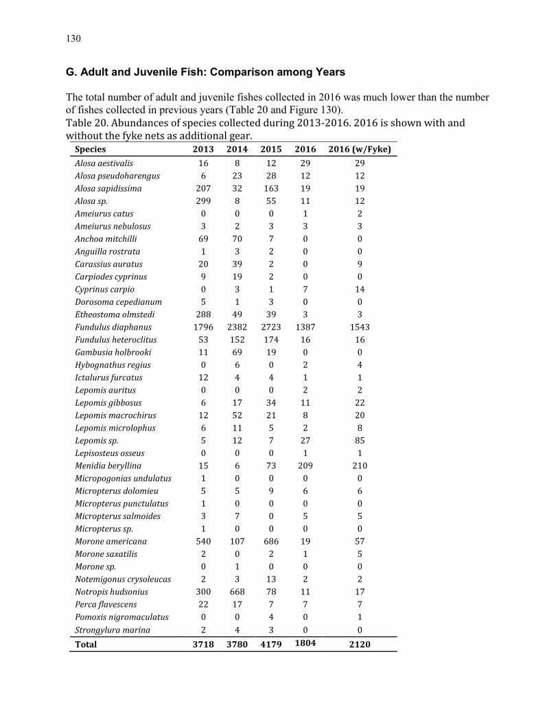
130

G. Adult and Juvenile Fish: Comparison among Years The total number of adult and juvenile fishes collected in 2016 was much lower than the number of fishes collected in previous years (Table 20 and Figure 130). Table 20. Abundances of species collected during 2013-2016. 2016 is shown with and without the fyke nets as additional gear.

Species 2013 2014 2015 2016 2016 (w/Fyke)

Alosa aestivalis 16 8 12 29 29

Alosa pseudoharengus 6 23 28 12 12

Alosa sapidissima 207 32 163 19 19

Alosa sp. 299 8 55 11 12

Ameiurus catus 0 0 0 1 2

Ameiurus nebulosus 3 2 3 3 3

Anchoa mitchilli 69 70 7 0 0

Anguilla rostrata 1 3 2 0 0

Carassius auratus 20 39 2 0 9

Carpiodes cyprinus 9 19 2 0 0

Cyprinus carpio 0 3 1 7 14

Dorosoma cepedianum 5 1 3 0 0

Etheostoma olmstedi 288 49 39 3 3

Fundulus diaphanus 1796 2382 2723 1387 1543

Fundulus heteroclitus 53 152 174 16 16

Gambusia holbrooki 11 69 19 0 0

Hybognathus regius 0 6 0 2 4

Ictalurus furcatus 12 4 4 1 1

Lepomis auritus 0 0 0 2 2

Lepomis gibbosus 6 17 34 11 22

Lepomis macrochirus 12 52 21 8 20

Lepomis microlophus 6 11 5 2 8

Lepomis sp. 5 12 7 27 85

Lepisosteus osseus 0 0 0 1 1

Menidia beryllina 15 6 73 209 210

Micropogonias undulatus 1 0 0 0 0

Micropterus dolomieu 5 5 9 6 6

Micropterus punctulatus 1 0 0 0 0

Micropterus salmoides 3 7 0 5 5

Micropterus sp. 1 0 0 0 0

Morone americana 540 107 686 19 57

Morone saxatilis 2 0 2 1 5

Morone sp. 0 1 0 0 0

Notemigonus crysoleucas 2 3 13 2 2

Notropis hudsonius 300 668 78 11 17

Perca flavescens 22 17 7 7 7

Pomoxis nigromaculatus 0 0 4 0 1

Strongylura marina 2 4 3 0 0

Total 3718 3780 4179 1804 2120

131

A clear contributor to the low numbers in 2016 was the difficulty in trawling AR3, and our inability to trawl there after mid-July. The reason for this is the extensive SAV (submerged aquatic vegetation) growth in Hunting Creek. There are clear benefits to the presence of SAV, it for example provides fish habitat and helps improve water clarity, but the excessive growth makes it difficult to sample fish. It should be noted that while the SAV growth is likely linked to the lower catches in 2016, it is more likely because of our inability to catch the fish, than that their numbers are that much reduced. To address this problem (we had seen the SAV growth increasing in previous years), we added fyke nets to our sampling gear in 2016. In general, fyke net catches are a bit lower than seine or trawl catches because it is passive gear rather than active gear (the fyke net is stationary and the fish will need to swim in). The extensive SAV growth made it highly suitable gear for the location, and total catch with fyke nets actually exceeded that of the trawls. However, even with fyke net catches included, total catch was much lower than previous years (Table 15). The fyke nets are likely to be the most efficient gear to sample thick SAV beds, and we recommend continued use of this gear in our surveys. In 2016 the clear trend of high abundances of Banded Killifish (Fundulus diaphanus) continues (Figure 130). Two other consistently abundant species, White Perch (Morone americana) and Spottail Shiner (Notropis hudsonius), were only present in low abundances in 2016, and Inland Silverside (Menidia beryllina) was the second most abundant species in 2016.

Figure 170. Percentage of total dominant species collected in 2013, 2014, 2015, and 2016.

0

0.1

0.2

0.3

0.4

0.5

0.6

0.7

0.8

0.9

1

2013 2014 2015 2016

Other

Menidia beryllina

Alosa sp.

Etheostoma olmstedi

Fundulus heteroclitus

Alosa sapidissima

Notropis hudsonius

Morone americana

Fundulus diaphanus

132

In 2016, 28 different species were collected, which is a sign of a healthy diversity. However, the high relative abundance of banded killifish results in very low evenness (distribution of abundance over species). This was apparent in previous years, but even more so in 2016. The Simpson’s Index (calculated as Σ (ni/N)2) was 0.27 in 2013, 0.43 in 2014, 0.45 in 2015, and 0.61 in 2016. Communities with higher diversity or evenness approach zero, and the higher catches of banded killifish in the samples reduce evenness. Evenness has been reduced each year of sampling, which is not something than is generally caused by gear obstructions. In addition, the fyke net collections are included in the percent dominance estimate of 2016 (Figure 130). This reducing trend in biodiversity, and potentially fish abundance, should be closely monitored. The shear presence of this high amount of banded killifishes is of course not a sign of low environmental quality; they generally require abundant aquatic vegetation to thrive, and Hunting Creek must be of healthy enough environmental quality to sustain submerged aquatic vegetation. Overall, the fish species found in Hunting Creek are characteristic of Potomac River tributaries. H. Submersed Aquatic Vegetation: Comparison among Years According to annual reports of the Virginia Institute of Marine Science (VIMS) SAV Monitoring Program (http://web.vims.edu/bio/sav/maps.html), virtually the entire surface area of the Hunting Creek embayment has been covered with submersed aquatic vegetation in each of the years of this study (2013-2016). In 2016 mapping of species was done in association with the water quality mapping surveys and the results have been reported in the results section of this report. In future years we plan to collect further data on species composition to allow for trend analysis of species abundances. I. Benthic Macroinvertebrates: Comparison among Years Benthic macroinvertebrate communities at the tidal stations (AR2, AR3, and AR4) exhibited similar patterns in all years sampled to date. Oligochaetes were most the most abundant group in 2016 as in all previous years. Chironomids were normally the second most abundant group in previous years, but in 2016 gastropods were second most abundant. As in previous years chironomids were most abundant at AR2. Gastropods have generally been most important at AR3 and that continued to be true in 2016. Amphipods were moderately abundant at all stations in 2016 as in previous years. There was a slightly higher diversity of different taxa of aquatic insects reported in 2016 than in previous years and in particular mayflies were more abundant although still relatively rare. Tributary benthic samples were collected for the first time in 2016 and these data will provide a baseline for assessment of future trends. Overall tributary stations exhibited moderately degraded conditions typical of streams draining urbanized areas such as the Cameron Run watershed.

http://web.vims.edu/bio/sav/maps.html

133

LITERATURE CITED Bigelow, H.B. and W.C.Schroeder. 1953. Fishes of the Gulf of Maine. Fishery bulletin No. 74,

Vol. 53. U.S. Government Printing Office. Washinton, D.C. 577 pp. Carter, V., P.T. Gammon, and N.C. Bartow. 1983. Submersed Aquatic Plants of the Tidal

Potomac River. Geological Survey Bulletin 1543. U.S. Geological Survey. 63 pp. Chesapeake Bay Program. 2006 Ambient water quality criteria for dissolved oxygen, water

clarity, and chlorophyll a for the Chesapeake Bay and its tidal tributaries. 2006 Addendum. Downloaded from Bay Program website 10/13/2006.

Cummings, H.S., W.C. Purdy, and H.P. Ritter. 1916. Investigations of the pollution and sanitary conditions of the Potomac watershed. Treasury Department, U.S. Public Health Service Hygienic Laboratory Bulletin 104. 231 pp.

Dahlberg, M.D. 1975. Guide to coastal fishes of Georgia and nearby states. University of Georgia Press. Athens, GA 187 pp.

Douglass, R.R. 1999. A Field Guide to Atlantic Coast Fishes: North America (Peterson Field Guides). Houghton Mifflin Harcourt, Boston. 368 pp.

Eddy, S. and J.C. Underhill. 1978. How to know the freshwater fishes. 3rd Ed. W.C. Brown Co. Dubuque, IA. 215 pp.

Froese, R. and D. Pauly (Eds.). 2012. Fish Base. World Wide Web electronic publication. www.fishbase.org, version (04/2012).

Hildebrand and Schroeder. 1928. Fishes of the Chesapeake Bay. U.S. Bureau of Fisheries Bulletin 53, Part 1. Reprinted 1972. T.F.H. Publishing, Inc. Neptune, NJ. 388 pp.

Hogue, J.J, Jr., R.Wallus, and L.K. Kay. 1976. Preliminary guide to the identification of larval fishes in the Tennessee River. Technical Note B19. Tennessee Valley Authority. Knoxville, TN.

Islam, S. 2001. Seasonal dynamics of micro-, nanno-, and picoplankton in the tidal freshwater Potomac River in and around Gunston Cove. Ph.Dissertation. George Mason University. 127 pp.

Jenkins, R.E. and N.M. Burkhead. 1994. The freshwater fishes of Virginia. American Fisheries Society. Washington, DC. 1080 pp.

Jones, P.W., F.D. Martin, and J.D. Hardy, Jr. 1978. Development of fishes of the Mid-Atlantic bight. Volumes I-VI. Fish and Wildlife Service, U.S. Department of the Interior. FWS/OBS-78/12.

Kraus, R.T. and R.C. Jones. 2011. Fish abundances in shoreline habitats and submerged aquatic vegetation in a tidal freshwater embayment of the Potomac River. Environmental Monitoring and Assessment. Online: DOI 10.1007/s10661-011-2192-6.

Kelso, D.W., R.C. Jones, and P.L. deFur. 1985. An ecological study of Gunston Cove - 1984-85. 206 pp.

Lippson, A.J. and R.L. Moran. 1974. Manual for identification of early development stages of fishes of the Potomac River estuary. Power Plant Siting Program, Maryland Department of Natural Resources. PPSP-MP-13.

Loos, J.J., W.S. Woolcott, and N.R. Foster. 1972. An ecologist’s guide to the minnows of the freshwater drainage systems of the Chesapeake Bay area. Association of Southeastern Biologists Bulletin 19: 126-138.

http://www.fishbase.org/

134

Lund, J.W.G., C. Kipling, and E.C. LeCren. 1958. The inverted microscope method of estimation algal numbers and the statistical basis of estimations by counting. Hydrobiologia 11: 143-170.

Mansueti, A.J. and J.D. Hardy, Jr. 1967. Development of fishes of the Chesapeake Bay region: an atlas of egg, larvae and juvenile stages: Part 1. Natural Resources Institute. University of Maryland. 202 pp.

Merritt, R.W. and K.W. Cummins. 1984. An introduction to the aquatic insects of North America. 2nd edition. Kendall/Hunt Publishing Co., Dubuque, IA. 722 pp.

Pennack, R.W. 1978. Fresh-water invertebrates of the United States. 2nd ed. Wiley-Interscience. New York, NY.

Schloesser, R.W., M.C. Fabrizio, R.J. Latour, G.C. Garman, G.C., B. Greenlee, M. Groves and J. Gartland. 2011. Ecological role of blue catfish in Chesapeake Bay communities and implications for management. American Fisheries Society Symposium 77:369-382.

Scott, W.B. and E.J. Crossman. 1973. Freshwater fishes of Canada. Bulletin 184. Fisheries Research Board of Canada. Ottawa, Canada. 966 pp.

Standard Methods for the Examination of Water and Wastewater. 1980. American Public Health Association, American Waterworks Association, Water Pollution Control Federation. 15th ed. 1134 pp.

Thorp, J.H. and A.P. Covich, eds. 1991. Ecology and classification of North American Freshwater Invertebrates. Academic Press. San Diego, CA. 911 pp.

Wetzel, R.G. 1983. Limnology. 2nd ed. Saunders. 767 pp. Wetzel, R.G. and G.E. Likens. 1991. Limnological analyses. 2nd ed. Springer-Verlag. 391 pp.

135

Anadromous Fish Survey Cameron Run 2016 Final Report

By

Kim de Mutsert

Assistant Professor, Department of Environmental Science and Policy George Mason University

Introduction The commercially valuable anadromous fishes in the herring family (Clupeidae) live as adults in the coastal ocean, but return to freshwater creeks and rivers to spawn. In the mid-Atlantic region, four species are present: American Shad (Alosa sapidissima), Blueback Herring (Alosa aestivalis), Alewife (Alosa pseudoharengus), and Hickory Shad (Alosa mediocris). Two other herring family species are semi-anadromous and spawn in Potomac River tributaries. These are Gizzard Shad (Dorosoma cepedianum) and Threadfin Shad (Dorosoma petenense). Both are very similar morphologically and ecologically, but only D. cepedianum is found as far upriver on the Potomac River watershed as Hunting Creek/Cameron Run. Previous reports describe the history of herring populations in the Potomac River watershed (Jones et al. 2014). The focus of the Cameron Run fish survey is river herring, the collective name of Blueback Herring and Alewife. River herring populations have declined drastically over their range, spurring conservation efforts since 1970, which have been intensified since 2005 with implementation of moratoria. Identifying all areas used as spawning habitat by Alewife and/or Blueback Herring is an important component of their conservation. Since 1988, George Mason University researchers have focused a monitoring program on the spawning of these species in other tributaries such as Pohick Creek, Accotink Creek, and, less regularly, Dogue Creek. With this study Cameron Run has been added, which has not been monitored for river herring or other anadromous species by either George Mason or other fisheries biologists before the start of this study in 2013 (Jim Cummins, pers. comm.). Our 2013 survey provided the first confirmation of Cameron Run as River Herring spawning habitat (Allan Weaver, VDGIF, pers. comm.). Use of Cameron Run by river herring upstream from the outfall of Alexandria Renew Enterprises signifies that the effluent does not deter river herring from using Cameron Run as spawning habitat. In 2014 we moved the collection site approximately 500 m downstream (still above the Alexandria Renew Enterprises effluent), which increased our catches, and allows us to estimate the size of the spawning population. The new location has proven successful and will remain the collection site for any subsequent surveys. Methods We conducted weekly sampling trips from March 23 to May 25 in 2016. During each trip a hoop net was set to completely block the creek allowing collection of adults swimming

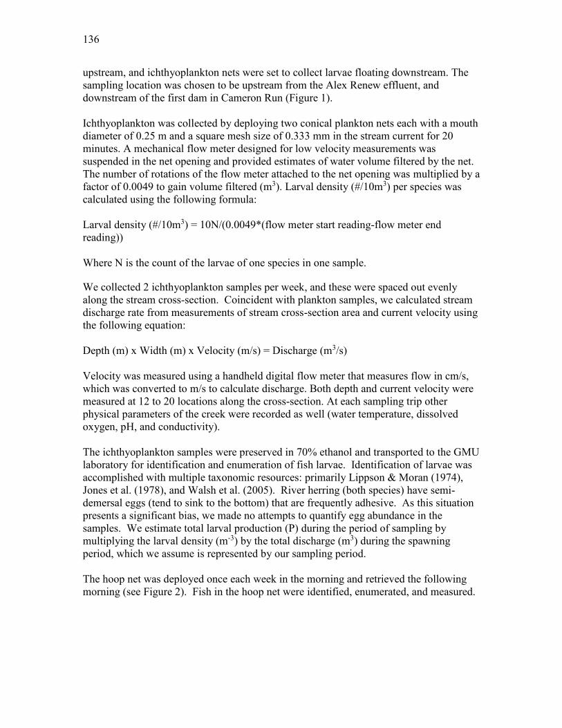
136

upstream, and ichthyoplankton nets were set to collect larvae floating downstream. The sampling location was chosen to be upstream from the Alex Renew effluent, and downstream of the first dam in Cameron Run (Figure 1). Ichthyoplankton was collected by deploying two conical plankton nets each with a mouth diameter of 0.25 m and a square mesh size of 0.333 mm in the stream current for 20 minutes. A mechanical flow meter designed for low velocity measurements was suspended in the net opening and provided estimates of water volume filtered by the net. The number of rotations of the flow meter attached to the net opening was multiplied by a factor of 0.0049 to gain volume filtered (m3). Larval density (#/10m3) per species was calculated using the following formula: Larval density (#/10m3) = 10N/(0.0049*(flow meter start reading-flow meter end reading)) Where N is the count of the larvae of one species in one sample. We collected 2 ichthyoplankton samples per week, and these were spaced out evenly along the stream cross-section. Coincident with plankton samples, we calculated stream discharge rate from measurements of stream cross-section area and current velocity using the following equation: Depth (m) x Width (m) x Velocity (m/s) = Discharge (m3/s) Velocity was measured using a handheld digital flow meter that measures flow in cm/s, which was converted to m/s to calculate discharge. Both depth and current velocity were measured at 12 to 20 locations along the cross-section. At each sampling trip other physical parameters of the creek were recorded as well (water temperature, dissolved oxygen, pH, and conductivity). The ichthyoplankton samples were preserved in 70% ethanol and transported to the GMU laboratory for identification and enumeration of fish larvae. Identification of larvae was accomplished with multiple taxonomic resources: primarily Lippson & Moran (1974), Jones et al. (1978), and Walsh et al. (2005). River herring (both species) have semi-demersal eggs (tend to sink to the bottom) that are frequently adhesive. As this situation presents a significant bias, we made no attempts to quantify egg abundance in the samples. We estimate total larval production (P) during the period of sampling by multiplying the larval density (m-3) by the total discharge (m3) during the spawning period, which we assume is represented by our sampling period. The hoop net was deployed once each week in the morning and retrieved the following morning (see Figure 2). Fish in the hoop net were identified, enumerated, and measured.

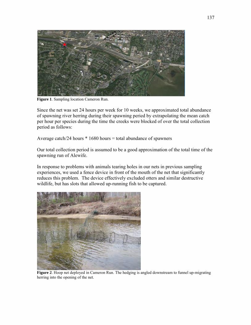
137

Figure 1. Sampling location Cameron Run. Since the net was set 24 hours per week for 10 weeks, we approximated total abundance of spawning river herring during their spawning peried by extrapolating the mean catch per hour per species during the time the creeks were blocked of over the total collection period as follows: Average catch/24 hours * 1680 hours = total abundance of spawners Our total collection period is assumed to be a good approximation of the total time of the spawning run of Alewife. In response to problems with animals tearing holes in our nets in previous sampling experiences, we used a fence device in front of the mouth of the net that significantly reduces this problem. The device effectively excluded otters and similar destructive wildlife, but has slots that allowed up-running fish to be captured.

Figure 2. Hoop net deployed in Cameron Run. The hedging is angled downstream to funnel up-migrating herring into the opening of the net.

138

Results and Discussion During the 10-week sampling period, we caught nineteen adult Alewife, and several non river herring species (Table 1). The abundance of river herring collected in 2016 was similar and slightly higher than 2015 (16 Alewife), which signifies the consistent use of Cameron Run as spawning ground. The net is set in such a way that fishes need to swim upstream into Cameron Run to be caught in the net, which is a behavior associated with spawning. Extrapolating over the time sampled, this could mean that the Alewife spawning population in 2016 consisted of 133 individuals (112 last year). We did not find adult Blueback Herring specimens in our collections this year. This is not unusual because we have only collected 1 in 2014. However, the presence of Blueback Herring larvae (Alosa aestivalis, Table 2) suggest that Blueback Herring are using Cameron Run as a spawning site again this year, even though we are unable to estimate the size of the spawning population. Sampling over multiple years will provide us with increasingly better estimates of the spawning population of Alewife and Blueback Herring in Cameron Run. Table 1. Species collected in Cameron Run with hoop net during weekly sampling from 3/23/16-5/25/16. River herring are indicated bold font. Date Species English name Count

4/13/16 Alosa_pseudoharengus Alewife 14

4/20/16 Dorosoma_cepedianum Gizzard Shad 1

4/20/16 Catostomus_commersonii White Sucker 1

4/27/16 Micropterus_salmoides Largemouth Bass 1

4/27/16 Lepomis_machrochirus Bluegill 2

4/27/16 Carassius_auratus Goldfish 1

5/4/16 Carpiodes_cyprinus Quillback 1

5/4/16 Alosa_pseudoharengus Alewife 5


5/4/16 Lepomis_machrochirus Bluegill 1 5/4/16 Morone_americana White Perch 10


In the ichthyoplankton samples we indeed found larvae of Alewife and well as Blueback Herring (Table 2). This year we found a total of 29 positively identified Alewife larvae and 4 Blueback Herring larvae in our samples. In addition, we found 1 Hickory Shad larvae, which is an alosid as well (Alosa mediocris). Larvae of other species were present in the samples as well, including, but not limited to, the semi-anadromous species White Perch (Morone americana; Table 2).

139

Table 2. Larvae collected in Cameron Run. Herring larvae (river herring and other clupeids) are in bold. Fish larvae too damaged for identification to species level were identified at the highest level possible. Date Species Count Volume

sampled

(m3)

Larval

density

(#/10m3)

3/23/16 Alosa pseudoharengus 2 24.83 0.81 3/23/16 Eggs 12 54.66 2.25 3/23/16 Unidentifiable 1 24.83 0.40 3/30/16 Eggs 19 56.12 3.87 4/6/16 Alosa mediocris 1 35.03 0.29 4/6/16 Alosa pseudoharengus 2 28.64 0.70 4/6/16 Cyprinidae 2 63.67 0.32 4/6/16 Eggs 3 63.67 0.46 3/23/16 Alosa pseudoharengus 2 24.83 0.81 4/6/16 Unidentifiable 1 35.03 0.29 4/20/16 Alosa pseudoharengus 9 76.98 1.16 4/20/16 Carassius auratus 3 37.49 0.80 4/20/16 Eggs 55 76.98 7.18 4/20/16 Notropis hudsonius 17 76.98 2.17 4/20/16 Unidentifiable 3 76.98 0.39 4/27/16 Alosa aestivalis 3 0.12* - 4/27/16 Alosa pseudoharengus 14 0.21* - 4/27/16 Eggs 2 0.21* - 5/4/16 Carpiodes cyprinus 1 61.66 0.16 5/4/16 Eggs 1230 115.93 105.52 5/4/16 Morone americana 3 54.27 0.55 5/4/16 Notropis hudsonius 1 61.66 0.16 5/4/16 Unidentifiable 3 115.93 0.27 5/11/16 Eggs 15 0.32* - 5/18/16 Alosa aestivalis 1 73.61 0.14 5/18/16 Alosa pseudoharengus 2 54.90 0.36 5/18/16 Dorosoma cepedianum 4 54.90 0.73 5/18/16 Eggs 11 128.51 0.79 5/18/16 Etheostoma olmstedi 1 73.61 0.14 5/18/16 Notropis hudsonius 3 128.51 0.25 5/18/16 Unidentifiable 2 128.51 0.16 5/25/16 Dorosoma cepedianum 1 0.16* - 5/25/16 Eggs 33 0.29* - 5/25/16 Morone americana 5 0.29* - 5/25/16 Unidentifiable 1 0.16* -

*The flow velocity in Cameron Run was too low at this date for the flow meter to function properly; therefore, volume sampled is likely an underestimate, and larval density not calculated. We measured creek discharge and other physical parameters at the same location and times where ichthyoplankton samples were taken, which was about 100 m downstream from the hoopnet (Table 3). Mean creek discharge was slightly lower compared to last

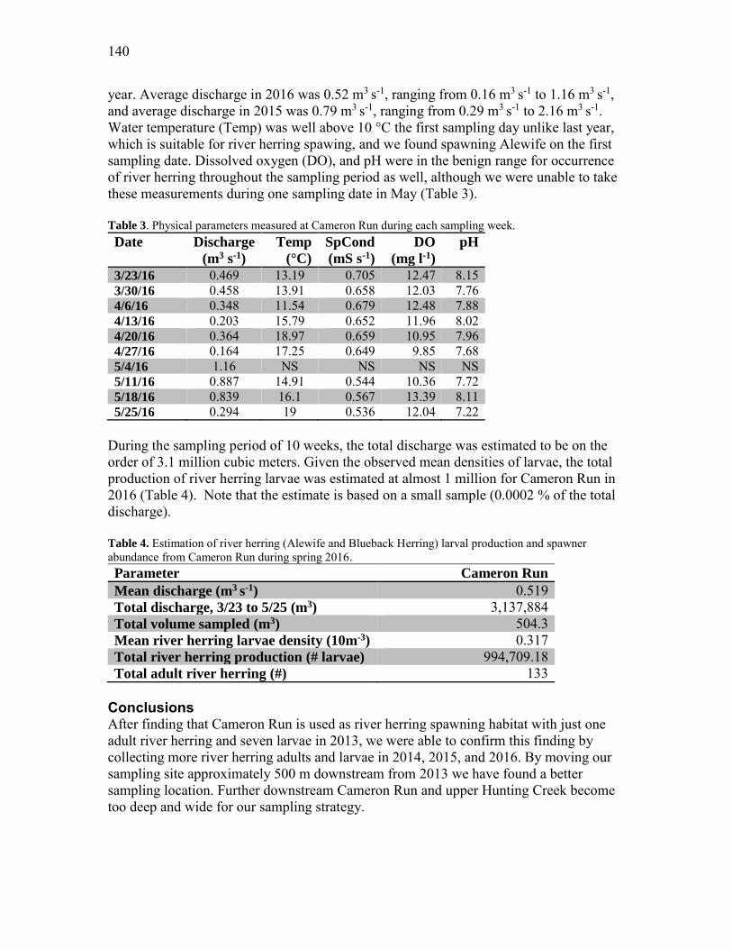
140

year. Average discharge in 2016 was 0.52 m3 s-1, ranging from 0.16 m3 s-1 to 1.16 m3 s-1, and average discharge in 2015 was 0.79 m3 s-1, ranging from 0.29 m3 s-1 to 2.16 m3 s-1. Water temperature (Temp) was well above 10 °C the first sampling day unlike last year, which is suitable for river herring spawing, and we found spawning Alewife on the first sampling date. Dissolved oxygen (DO), and pH were in the benign range for occurrence of river herring throughout the sampling period as well, although we were unable to take these measurements during one sampling date in May (Table 3). Table 3. Physical parameters measured at Cameron Run during each sampling week. Date Discharge

(m3 s-1)

Temp

(°C)

SpCond

(mS s-1)

DO

(mg l-1)

pH

3/23/16 0.469 13.19 0.705 12.47 8.15 3/30/16 0.458 13.91 0.658 12.03 7.76 4/6/16 0.348 11.54 0.679 12.48 7.88 4/13/16 0.203 15.79 0.652 11.96 8.02 4/20/16 0.364 18.97 0.659 10.95 7.96 4/27/16 0.164 17.25 0.649 9.85 7.68 5/4/16 1.16 NS NS NS NS 5/11/16 0.887 14.91 0.544 10.36 7.72 5/18/16 0.839 16.1 0.567 13.39 8.11 5/25/16 0.294 19 0.536 12.04 7.22

During the sampling period of 10 weeks, the total discharge was estimated to be on the order of 3.1 million cubic meters. Given the observed mean densities of larvae, the total production of river herring larvae was estimated at almost 1 million for Cameron Run in 2016 (Table 4). Note that the estimate is based on a small sample (0.0002 % of the total discharge). Table 4. Estimation of river herring (Alewife and Blueback Herring) larval production and spawner abundance from Cameron Run during spring 2016. Parameter Cameron Run

Mean discharge (m3 s-1) 0.519 Total discharge, 3/23 to 5/25 (m3) 3,137,884 Total volume sampled (m3) 504.3 Mean river herring larvae density (10m-3) 0.317 Total river herring production (# larvae) 994,709.18 Total adult river herring (#) 133

Conclusions After finding that Cameron Run is used as river herring spawning habitat with just one adult river herring and seven larvae in 2013, we were able to confirm this finding by collecting more river herring adults and larvae in 2014, 2015, and 2016. By moving our sampling site approximately 500 m downstream from 2013 we have found a better sampling location. Further downstream Cameron Run and upper Hunting Creek become too deep and wide for our sampling strategy.

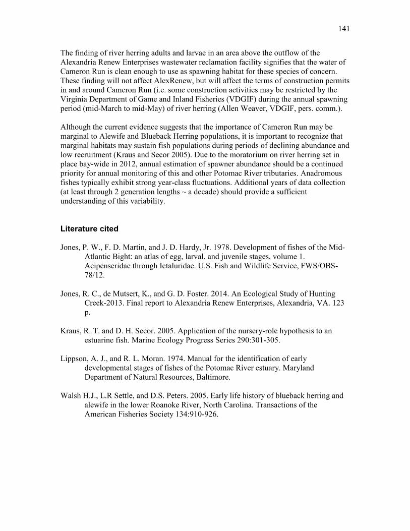
141

The finding of river herring adults and larvae in an area above the outflow of the Alexandria Renew Enterprises wastewater reclamation facility signifies that the water of Cameron Run is clean enough to use as spawning habitat for these species of concern. These finding will not affect AlexRenew, but will affect the terms of construction permits in and around Cameron Run (i.e. some construction activities may be restricted by the Virginia Department of Game and Inland Fisheries (VDGIF) during the annual spawning period (mid-March to mid-May) of river herring (Allen Weaver, VDGIF, pers. comm.). Although the current evidence suggests that the importance of Cameron Run may be marginal to Alewife and Blueback Herring populations, it is important to recognize that marginal habitats may sustain fish populations during periods of declining abundance and low recruitment (Kraus and Secor 2005). Due to the moratorium on river herring set in place bay-wide in 2012, annual estimation of spawner abundance should be a continued priority for annual monitoring of this and other Potomac River tributaries. Anadromous fishes typically exhibit strong year-class fluctuations. Additional years of data collection (at least through 2 generation lengths ~ a decade) should provide a sufficient understanding of this variability.

Literature cited Jones, P. W., F. D. Martin, and J. D. Hardy, Jr. 1978. Development of fishes of the Mid-

Atlantic Bight: an atlas of egg, larval, and juvenile stages, volume 1. Acipenseridae through Ictaluridae. U.S. Fish and Wildlife Service, FWS/OBS-78/12.

Jones, R. C., de Mutsert, K., and G. D. Foster. 2014. An Ecological Study of Hunting Creek-2013. Final report to Alexandria Renew Enterprises, Alexandria, VA. 123 p.

Kraus, R. T. and D. H. Secor. 2005. Application of the nursery-role hypothesis to an estuarine fish. Marine Ecology Progress Series 290:301-305.

Lippson, A. J., and R. L. Moran. 1974. Manual for the identification of early

developmental stages of fishes of the Potomac River estuary. Maryland Department of Natural Resources, Baltimore.

Walsh H.J., L.R Settle, and D.S. Peters. 2005. Early life history of blueback herring and

alewife in the lower Roanoke River, North Carolina. Transactions of the American Fisheries Society 134:910-926.

143

Escherichia coli abundances in Hunting Creek/Cameron Run

and adjacent Potomac River - 2016 Final Report Submitted by Robert B. Jonas

Associate Professor, Department of Environmental Science and Policy GEORGE MASON UNIVERSITY 4400 UNIVERSITY DRIVE FAIRFAX, VA 22030 to ALEXANDRIA RENEW ENTERPRISES

Alexandria, Virginia Submitted: March 20, 2017

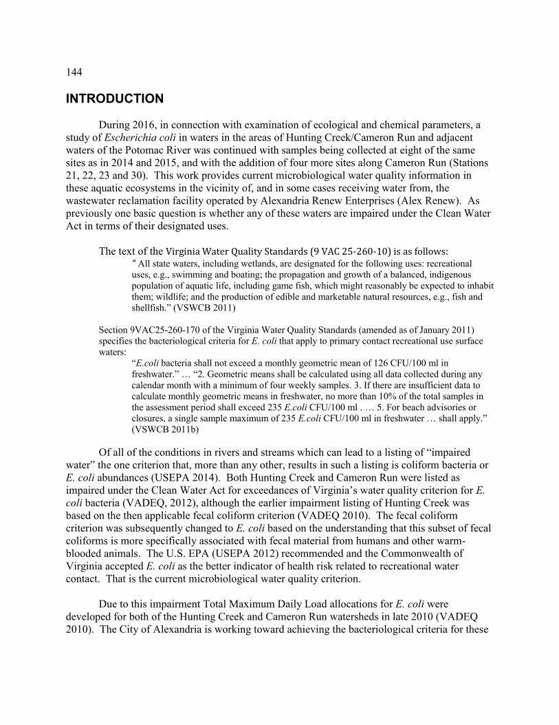
144

INTRODUCTION During 2016, in connection with examination of ecological and chemical parameters, a study of Escherichia coli in waters in the areas of Hunting Creek/Cameron Run and adjacent waters of the Potomac River was continued with samples being collected at eight of the same sites as in 2014 and 2015, and with the addition of four more sites along Cameron Run (Stations 21, 22, 23 and 30). This work provides current microbiological water quality information in these aquatic ecosystems in the vicinity of, and in some cases receiving water from, the wastewater reclamation facility operated by Alexandria Renew Enterprises (Alex Renew). As previously one basic question is whether any of these waters are impaired under the Clean Water Act in terms of their designated uses. The text of the Virginia Water Quality Standards (9 VAC 25-260-10) is as follows: “ All state waters, including wetlands, are designated for the following uses: recreational

uses, e.g., swimming and boating; the propagation and growth of a balanced, indigenous population of aquatic life, including game fish, which might reasonably be expected to inhabit them; wildlife; and the production of edible and marketable natural resources, e.g., fish and shellfish.” (VSWCB 2011)

Section 9VAC25-260-170 of the Virginia Water Quality Standards (amended as of January 2011)

specifies the bacteriological criteria for E. coli that apply to primary contact recreational use surface waters:

“E.coli bacteria shall not exceed a monthly geometric mean of 126 CFU/100 ml in freshwater.” … “2. Geometric means shall be calculated using all data collected during any calendar month with a minimum of four weekly samples. 3. If there are insufficient data to calculate monthly geometric means in freshwater, no more than 10% of the total samples in the assessment period shall exceed 235 E.coli CFU/100 ml . … 5. For beach advisories or closures, a single sample maximum of 235 E.coli CFU/100 ml in freshwater … shall apply.”

(VSWCB 2011b) Of all of the conditions in rivers and streams which can lead to a listing of “impaired water” the one criterion that, more than any other, results in such a listing is coliform bacteria or E. coli abundances (USEPA 2014). Both Hunting Creek and Cameron Run were listed as impaired under the Clean Water Act for exceedances of Virginia’s water quality criterion for E. coli bacteria (VADEQ, 2012), although the earlier impairment listing of Hunting Creek was based on the then applicable fecal coliform criterion (VADEQ 2010). The fecal coliform criterion was subsequently changed to E. coli based on the understanding that this subset of fecal coliforms is more specifically associated with fecal material from humans and other warm-blooded animals. The U.S. EPA (USEPA 2012) recommended and the Commonwealth of Virginia accepted E. coli as the better indicator of health risk related to recreational water contact. That is the current microbiological water quality criterion. Due to this impairment Total Maximum Daily Load allocations for E. coli were developed for both of the Hunting Creek and Cameron Run watersheds in late 2010 (VADEQ 2010). The City of Alexandria is working toward achieving the bacteriological criteria for these

145

waters through a variety of programs including a storm water program, minimizing combined storm water sewer system overflows, reductions in pet waste sources and discovery of illegal discharges. Because the sources of E. coli to water systems are many and varied, including wildlife sources which are generally not controlled unless at a nuisance level, continued monitoring of E. coli in these waterways is an important aspect of maintaining and improving water quality. The results reported here add to the understanding of the microbiological quality of these systems. METHODS Sampling Regime: Samples were collected on eleven dates from 27 April 2016 to 22 September 2016 on a semimonthly basis (Table EC1). Water samples were collected at twelve stations on each sampling date. Station identifiers and locations are shown in Table EC2 (map of EC sample sites in Appendix A, Figure A1). In this report we will consider the Telegraph Rd. bridge as the dividing line between Cameron Run and upper Hunting Creek; this conforms with Virginia Department of Environmental Quality designations. Samples were collected in clean, steam sterilized (autoclaved), 4 liter, wide-mouth polypropylene bottles. Eight of the stations were approached from the shore and four were sampled from a small, outboard powered research vessel. Of the shore-approached stations AR11 was sampled on the upstream (lake) side of the dam at Lake Cook approximately 10 meters from the shore. In this case only the sampling equipment came in contact with the lake water. Similarly at station AR1 samples were collected remotely using a sterilized, 4 liter round polypropylene wide-mouth bottle fitted with a harness and nylon line. The sample bottle was deployed from atop the George Washington Parkway Bridge over Hunting Creek on the upstream side approximately at mid-span. The bottle was rinsed twice with sample water and then the final sample was collected. Collection of the remaining two shore-approached samples required wading in the streams. At AR12 we waded into the water downstream of the collection site, waited for the current to carry away any disturbed sediment and then collected the sample by submerging the 4 liter bottle upstream of the sample collector. At AR 13 the bottom of the stream at the approach site is paved with concrete. At this site we waded to approximately midstream and to the edge of the concrete paved segment. After waiting for any disturbed sediment to be washed away the sampled was collected again by submerging the sterile 4 liter bottle in the stream. Boat-approached sites were sampled by submerging the collection bottles over the side of the research vessel as the vessel coasted to its anchorage. Immediately after collection, samples were placed in dark, insulated containers and chilled with ice. Samples were returned to the George Mason University (Mason), Fairfax campus where they were processed within about 5 hours of collection.

Analytical Method: Determination of the abundance of E. coli followed the EPA Method 1603 (Escherichia coli in Water by Membrane Filtration Using Modified membrane-Thermotolerant Escherichia coli Agar (Modified mTEC)). This is an EPA-approved method for determining abundance of E. coli in fresh water. It is a one-step modification of the EPA Method 1103.1. It is based on E. coli production β-Dglucuronidase and the consequent metabolism of 5-bromo-6-

146

chloro-3-indolyl-β-D-glucuronide in the medium to glucuronic acid and a red- or magenta-colored product (USEPA 2009).

Table EC1: Sampling Dates

Date Date Code for figures

27-Apr-16 20160427

10May-16 20160510

25-May-16 20160525

08-Jun-16 20160608

23-Jun-16 20160623

07-Jul-16 20160707

25-Jul-16 20160725

08-Aug-16 20160808

22-Aug-16 20160822

06-Sep-16 20160906

22-Sep-16 20160922

Table EC2: Station identifiers, locations and access type.

Station ID Access Type Location Description Latitude Longitude

AR 1 Shore Hunting Cr at the GW Parkway Bridge 38o 47.40' N 77o 03.09' W

AR 2 Boat Northern portion of Hunting Cr. 38o 47.10' N 77o 02.95' W

AR 3 Boat Southern portion of Hunting Cr. 38o 46.93' N 77o 02.89' W

AR 4 Boat Potomac River Channel off Hunting Cr. 38o 46.88' N 77o 02.04' W

AR 10 Boat Potomac River North of Wilson Bridge 38o 47.65' N 77o 02.34' W

AR 11 Shore Outlet of Lake Cook 38o 48.26' N 77o 05.85' W

AR 12 Shore Last Riffle of Cameron Run near Beltway crossing 38o 48.11' N 77o 05.07' W

AR 13 Shore Hoff's Run upstream of Alex renew outfall 38o 48.17' N 77o 03.50' W

AR 21 Shore South side of Cameron Run downstream from Lake Cook drain 38o 48.19' N 77o 05.73' W

AR 22 Shore South side of upper Hunting Creek at north end of Fenwick Dr. 38o 47.87' N 77o 04.26' W

AR 23 Shore South side of upper Hunting Creek across from AlexRenew outfall 38o 47.62' N 77o 03.58' W

AR 30 Shore Cameron Run upstream near metro rail bridge 38o 48.32' N 77o 06.44' W

147

For this work mTEC medium (Fisher) was prepared in our laboratory at George Mason

University shortly before each sampling trip. The medium was prepared as per package directions, and 5 ml of the molten medium was placed aseptically into sterile, 50 mm Petri dishes with tight fitting lids. Prepared medium was stored at 4◦C in the dark until use. Phosphate buffered saline (PBS) was prepared as per Method 1603 and autoclave sterilized. PBS was added to smaller samples (1.0 ml and 10 ml) to make volumes up to at least 20 ml before filtration. This aids in distributing bacteria uniformly across the membrane surface. The PBS was also used for blank controls. Upon return to the laboratory, samples were processed immediately. Sterile, gridded, 0.45 µm membrane filters were aseptically positioned, grid side up, on the base of a sterile, polycarbonate filter holder, and the filter tower was placed in position on a vacuum flask over the filter and base. Samples were shaken vigorously to assure completely mixing and appropriate volumes (1.0 ml, 10.0 ml, 50.0 ml or 100.0 ml) of sample were added to each of three replicate filter systems. Before adding the two smaller volume aliquats to the filter funnels sufficient PBS was added to make the final volume approximately 20 ml. Samples were then filtered with vacuum (approximately 10 in Hg). Each filter was then removed from the filter holder base aseptically with sterile, blunt-tipped forceps and placed onto the surface of the mTEC agar without trapping any air bubbles beneath the filter. After replacing the Petri dish tops the plates were incubated inverted in a 35◦C incubator for 2 ± 0.5 hours. They were then removed, placed in tightly closed zipper-locked plastic bags and submerged in a water bath at 44.5°C ± 0.2°C for 22 ± 2 hours. Blank controls consisting of 100 ml of PBS were checked each time samples were processed. Generally no E. coli were detected in these blank controls, although occasionally one or two of the controls had one or two presumptive E. coli colonies. The data were not corrected for this low background as it was generally less than 1 percent of the abundances on countable plates. After the water bath incubation, samples were retrieved and observed immediately for typical red or magenta E. coli colonies. All Petri dishes (3 volumes x 3 replicates = 9 Petri dishes per sample) were observed. Although only dilutions yielding colony counts between 20 and 80 needed to be enumerated, we generally recorded colonies for each countable dilution. Often, however, when E. coli were abundant the higher volume samples were not countable due to overgrowth. Calculation of final E. coli abundances followed the procedures described in Appendix B of the EPA Method 1603 (USEPA 2009). Since there were triplicate analyses of each dilution the colony count per Petri dish was separately converted to E. coli abundance per 100 ml and then the triplicates were averaged. If no dilution gave individual counts between 20 and 80 the dilution that resulted in counts nearest to that range were selected and used for the final calculation as described in appendix B of the EPA Method 1603. RESULTS

Typical E. coli colonies were observed in some dilution in every sample tested. Therefore there is a point estimate of E. coli per 100ml for each. E. coli abundances by station are shown in Figures EC1 and EC2 (tabular data is in Appendix A, Table A1). Dates are coded

148

in reverse order for sorting purposes (e.g. 27 April 2016 = 20160427). For clarity only two stations are represented in each “by date” figure (Figures EC3 – EC8) and the station locations and relationships between stations are described in the figure legends.

Since there was no situation in which 4 weekly samples were collected in a calendar

month the 235 per 100 mL criterion is applicable in determining impairment. In contrast to the 2014 situation, when at four of the eight stations (sampled in that year) (AR11, 10, 3 and 4) thermotolerant E. coli abundances never exceeded 235 per 100 ml, in 2016 E. coli abundances exceed the 235 per 100 mL “impaired water” criterion at all stations sometime during the sampling period as they did in 2015. All four of the newly sampled stations (A21, 22, 23 and 30) also exceeded that criterion. In 2016 AR1 exceeded the 235 per 100 mL level on 8 of the 11 samples throughout the spring and summer. Stations 11, 12, 13, 21, 22, 23 and 30 all exceeded this criterion on nine or more of the sample dates. Station AR4 in the Potomac River exceeded the criterion on 2 of the 11 sample dates.

Thermotolerant E. coli abundance at Station AR13 (Hoff’s Run) exceeded 235 per 100

mL on all eleven dates from April through the end of September, as it did in 2015. The average E. coli at AR13 was over 4,450 per 100 mL and the maximum value was greater than 21,500 per 100 mL on 23 June. This was the highest value found during 2016. All of the stations, even those in the off-shore Potomac, sampled on 23 June exceeded the 235 per 100 mL criterion.

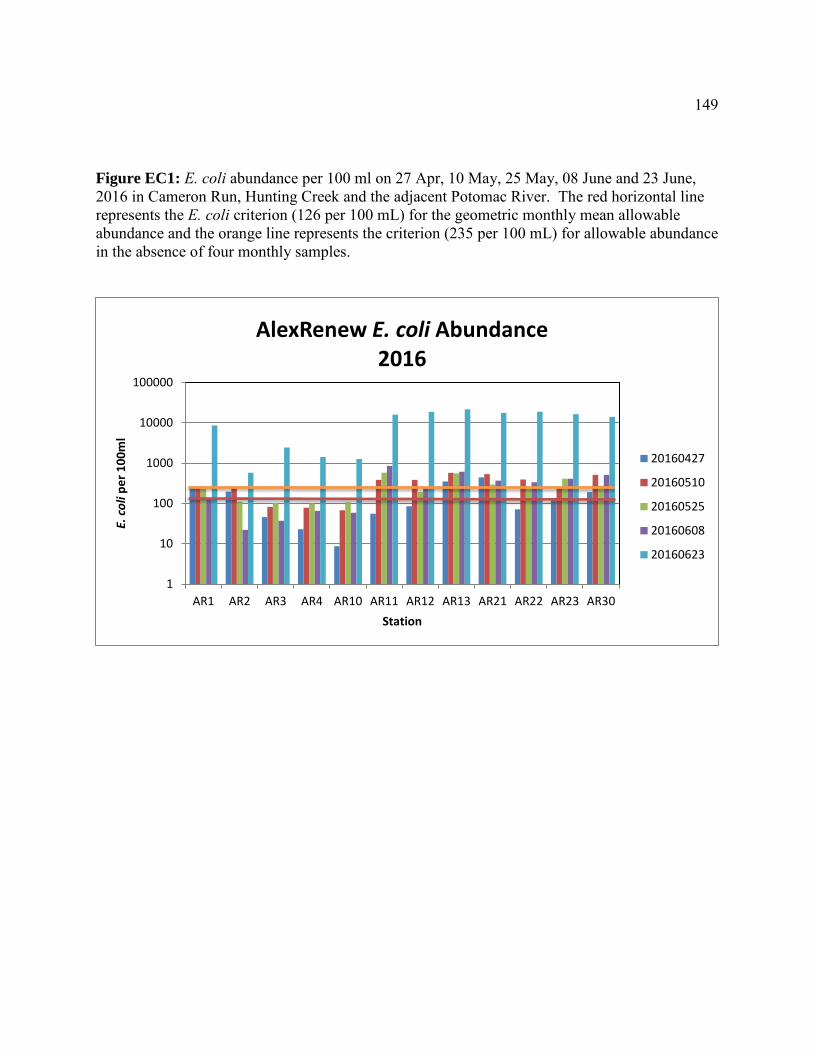
149

Figure EC1: E. coli abundance per 100 ml on 27 Apr, 10 May, 25 May, 08 June and 23 June, 2016 in Cameron Run, Hunting Creek and the adjacent Potomac River. The red horizontal line represents the E. coli criterion (126 per 100 mL) for the geometric monthly mean allowable abundance and the orange line represents the criterion (235 per 100 mL) for allowable abundance in the absence of four monthly samples.

1

10

100

1000

10000

100000

AR1 AR2 AR3 AR4 AR10 AR11 AR12 AR13 AR21 AR22 AR23 AR30

E. c

oli

pe

r 1

00

ml

Station

AlexRenew E. coli Abundance2016

20160427

20160510

20160525

20160608

20160623

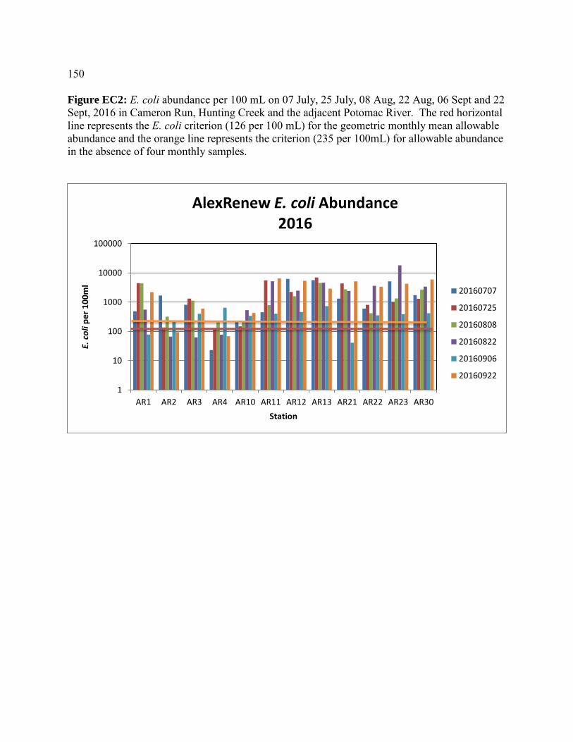
150

Figure EC2: E. coli abundance per 100 mL on 07 July, 25 July, 08 Aug, 22 Aug, 06 Sept and 22 Sept, 2016 in Cameron Run, Hunting Creek and the adjacent Potomac River. The red horizontal line represents the E. coli criterion (126 per 100 mL) for the geometric monthly mean allowable abundance and the orange line represents the criterion (235 per 100mL) for allowable abundance in the absence of four monthly samples.

1

10

100

1000

10000

100000

AR1 AR2 AR3 AR4 AR10 AR11 AR12 AR13 AR21 AR22 AR23 AR30

E. c

oli

pe

r 1

00

ml

Station


20160707

20160725

20160808

20160822

20160906

20160922

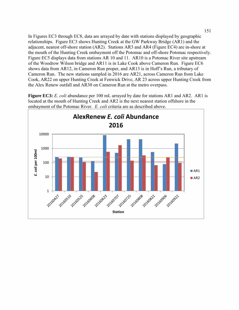
151

In Figures EC3 through EC8, data are arrayed by date with stations displayed by geographic relationships. Figure EC3 shows Hunting Creek at the GW Parkway Bridge (AR1) and the adjacent, nearest off-shore station (AR2). Stations AR3 and AR4 (Figure EC4) are in-shore at the mouth of the Hunting Creek embayment off the Potomac and off-shore Potomac respectively. Figure EC5 displays data from stations AR 10 and 11. AR10 is a Potomac River site upstream of the Woodrow Wilson bridge and AR11 is in Lake Cook above Cameron Run. Figure EC6 shows data from AR12, in Cameron Run proper, and AR13 is in Hoff’s Run, a tributary of Cameron Run. The new stations sampled in 2016 are AR21, across Cameron Run from Lake Cook, AR22 on upper Hunting Creek at Fenwick Drive, AR 23 across upper Hunting Creek from the Alex Renew outfall and AR30 on Cameron Run at the metro overpass.

Figure EC3: E. coli abundance per 100 mL arrayed by date for stations AR1 and AR2. AR1 is located at the mouth of Hunting Creek and AR2 is the next nearest station offshore in the embayment of the Potomac River. E. coli criteria are as described above.

1

10

100

1000

10000

E. c

oli

pe

r 1

00

ml

Station


AR1

AR2

152

Figure EC4: E. coli abundance per 100ml arrayed by date for stations AR3 and AR4. AR4 is an off-shore Potomac River mainstem channel station while AR3 is in-shore in the southern portion Hunting Creek embayment. E. coli criteria are as described above.

1

10

100

1000

10000

E. c

oli

pe

r 1

00

ml

Station


AR3

AR4

153

Figure EC5: E. coli abundance per 100ml arrayed by date for stations AR10 and AR11. AR10 is a Potomac River mainstem station north of the Wilson Bridge. AR11 is above the dam at Cook Lake on a tributary of Cameron Run. E. coli criteria are as described above.

1

10

100

1000

10000

100000

E. c

oli

pe

r 1

00

ml

Station


AR10

AR11

154

Figure EC6: E. coli abundance per 100 mL arrayed by date for stations AR12 and AR13. AR12 is a Cameron Run station just above head of tide and near Oak Park and AR 13 is located in Hoff’s Run upstream from the Alex Renew outfall. E. coli criteria are as described above.

1

10

100

1000

10000

100000

E. c

oli

pe

r 1

00

ml

Station


AR12

AR13

155

Figure EC7: E. coli abundance per 100 mL arrayed by date for stations AR21 and 22. AR21 is a Cameron Run station on the south side across Lake Cook and AR22 is on the south side of upper Hunting Creek at the end of Fenwick Dr. E. coli criteria are as described above.

1

10

100

1000

10000

100000

E. c

oli

pe

r 1

00

ml

Station


AR21

AR22

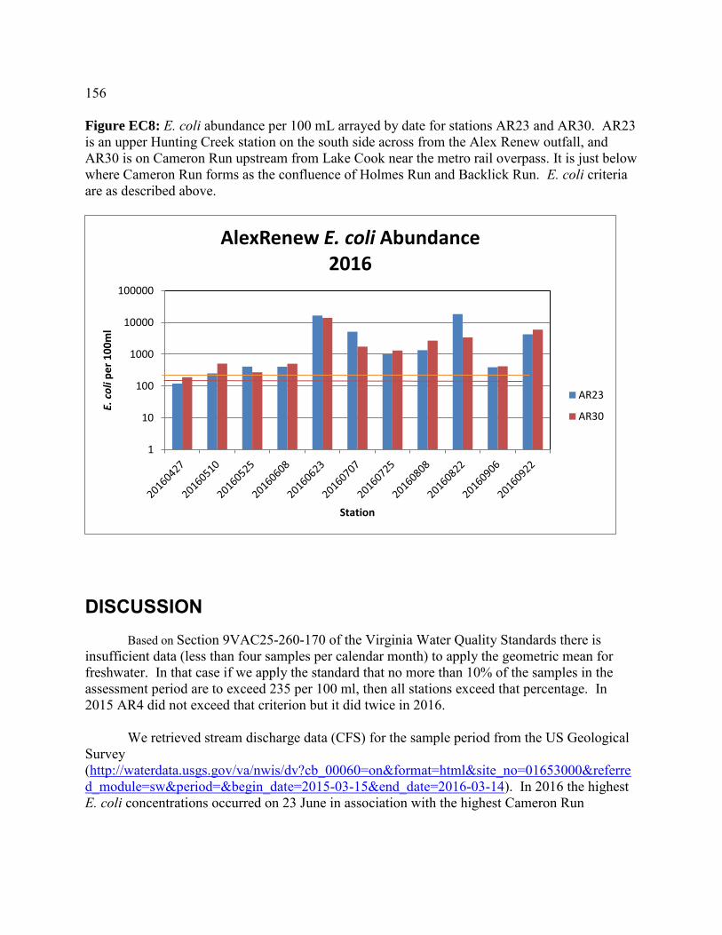
156

Figure EC8: E. coli abundance per 100 mL arrayed by date for stations AR23 and AR30. AR23 is an upper Hunting Creek station on the south side across from the Alex Renew outfall, and AR30 is on Cameron Run upstream from Lake Cook near the metro rail overpass. It is just below where Cameron Run forms as the confluence of Holmes Run and Backlick Run. E. coli criteria are as described above.

DISCUSSION

Based on Section 9VAC25-260-170 of the Virginia Water Quality Standards there is insufficient data (less than four samples per calendar month) to apply the geometric mean for freshwater. In that case if we apply the standard that no more than 10% of the samples in the assessment period are to exceed 235 per 100 ml, then all stations exceed that percentage. In 2015 AR4 did not exceed that criterion but it did twice in 2016.

We retrieved stream discharge data (CFS) for the sample period from the US Geological

Survey (http://waterdata.usgs.gov/va/nwis/dv?cb_00060=on&format=html&site_no=01653000&referred_module=sw&period=&begin_date=2015-03-15&end_date=2016-03-14). In 2016 the highest E. coli concentrations occurred on 23 June in association with the highest Cameron Run

1

10

100

1000

10000

100000

E. c

oli

pe

r 1

00

ml

Station


AR23

AR30

http://waterdata.usgs.gov/va/nwis/dv?cb_00060=on&format=html&site_no=01653000&referred_module=sw&period=&begin_date=2015-03-15&end_date=2016-03-14

http://waterdata.usgs.gov/va/nwis/dv?cb_00060=on&format=html&site_no=01653000&referred_module=sw&period=&begin_date=2015-03-15&end_date=2016-03-14

157

streamflow on any of the sampling dates. We explored the relationship between E. coli abundance and Cameron Run stream flow (Figures 9-14).

Figure EC9: E. coli at Cameron Run and upper Hunting Creek stations (AR12, 21, 22, 23 and 30) versus Stream Flow in Cameron Run on the date of sample collection. R2 is for the linear regression.

Figure EC10: E. coli at Cameron Run and upper Hunting Creek stations (AR12, 21, 22, 23 and 30) versus Stream Flow in Cameron Run on the date of sample collection. R2 is for the linear regression. Data from 23 June 2016 was excluded to explore more normal stream flow conditions. Stream flow on 23 June was 6 times greater than the overall mean stream flow and more than 10 times greater than mean flow with the 23 June value excluded.

It is clear that the exceptionally high stream flow (142 cfs) on 23 June 2016 was associated with exceptiomally high E. coli abundances on that day (Figure EC9). The average E. coli per 100 ml on 23 June among the five Cameron Run and upper Hunting Creek stations exceeded 17,000, and the lowest among them was 14,000 at Station 30 located farthest upstream. However, when the high stream flow values for 23 June were deleted, stream flows below about

R² = 0.7004

0

5000

10000

15000

20000

0 50 100 150

E co

li p

er

10

0m

l

Stream Flow in Cameron Run (cfs)

Cameron Run E. coli vs Stream Flow on Sample Date

Cameron Run

R² = 0.0129

0

5000

10000

15000

20000

0 10 20 30

E co

li p

er

10

0m

l


Cameron Run (exc 23 June, 2016) E. coli vs Stream Flow on Sample Date

Cameron Run

158

25 cfs in Cameron Run were not associated with statistically (R2 of only 0.01) increased E. coli abundances (Figure EC10). However, on 22 August there was an exceptionally high E. coli abundance of over 18,000 per 100 ml at Station AR23 (the down stream station: upper Hunting Creek across from the AlexRenew outfall) when the stream flow was 23 cfs, which is relatively high for Cameron Run on our sample collection dates when it averaged 11.9 cfs (excluding 23 June). Overall during the sample period (27 April to 22 September) stream flow averged about 32 cfs. The E. coli abundances in the Potomac River stations (Figures EC11 and EC12) were slightly positvely correlated with Cameron Run stream flow when the 23 June (high flow) data were included, but were not related to stream flow when the 23 June data were removed. The highest value for Potomac River stations, 8600 per 100ml (Figure EC11), was at AR1 at the mouth of Hunting Creek (where that joins with the Potomac River). The two high values shown in Figure EC12 (>4000 per 100 ml) were also at station AR1 but under low flow rates of 5.3 and 7.1 cfs.

Figure EC11: E. coli at Potomac River mainstem and Hunting Creek embayment stations (AR1, 2, 3, 4 and 10) versus Stream Flow in Cameron Run on the date of sample collection. R2 is for the linear regression.

R² = 0.2026

0100020003000400050006000700080009000

10000

0 50 100 150

E co

li p

er

10

0m

l


Potomac River E. coli vs Stream Flow on Sample Date

Potomac River

Linear (Potomac River)

159

Figure EC12: E. coli at Potomac River mainstem and Hunting Creek embayment stations (AR1, 2, 3, 4 and 10) versus Stream Flow in Cameron Run on the date of sample collection. R2 is for the linear regression. Data from 23 June 2016 was excluded here to explore more normal stream flow conditions. Stream flow on 23 June was 6 times greater than the overall mean stream flow and more than 10 times greater than mean flow with the 23 June value excluded.

When all data were included E. coli abundances at Lake Cook and at Hooff run were significantly associated with stream flow in Cameron Run (Figure EC 13). Both stations are tributaries of Cameron Run and were influenced by the excessive runoff that was observed on 23 June. As in other stations, if the 23 June stream flow values were excluded then there is no significant correlation between stream flow and E. coli (Figure EC14). In Hooff Run, which always exceeded the 235 per 100 m standard (was impaired) high values exceeding 4000 per 100ml occurred even at low (Cameron Run) stream flows of about 6 cfs.

Figure EC13: E. coli at Lake Cook and Hooff Run stations (AR11 and 12) versus Stream Flow in Cameron Run on the date of sample collection. R2 is for the linear regression.

R² = 0.0747

0

1000

2000

3000

4000

5000

0 10 20 30

E co

li p

er

10

0m

l


Potomac River (exc 23 June 2016)E. coli vs Stream Flow on Sample Date

Potomac River

R² = 0.718

R² = 0.8046

0

5000

10000

15000

20000

25000

0 50 100 150

E. c

oli

pe

r 1

00

mll


Lake Cook , Hooff RunE. coli vs Stream Flow on Sample Date

Lake Cook AR11

Hooff Run AR13

Linear (Lake Cook AR11)

Linear (Hooff Run AR13)

160

Figure EC14: E. coli at Lake Cook and Hooff Run stations (AR11 and 12) versus Stream Flow in Cameron Run on the date of sample collection. R2 is for the linear regression. Data from 23 June 2016 was excluded here to explore more normal stream flow conditions. Stream flow on 23 June was 6 times greater than the overall mean stream flow and more than 10 times greater than mean flow with the 23 June value excluded.

In 2015 higher E. coli values seemed to occur some time after (e.g. a day later) elevated stream flow especially when that elevated flow followed a period of low flow. There was not a simple linear (statistically significant) relationship between E. coli abundance and the previous day’s stream flow, but the highest abundance occurred on the day following increased stream flow. Similarly data from 2016 do not suggests a simple linear relationship between E. coli abundance and Cameron Run stream flow even when considering only stations located along the mainstem of Cameron Run. Therefore, we explored relationships of stream flow on days prior to sampling and E. coli on the sampling date.

Because the 2105 data suggested that stream flow on the day prior to sampling might be

relate to E. coli abundance, Figure 15 show E. coli plotted against stream flow on the day prior to sample collection (for these analyses only data from Stations 12, 21, 22, 23 and 30 arrayed along Cameron Run were evaluated). Bacterial abundance and stream flow were not significantly associated under this test. In fact the data suggest very high abundances associated with lower stream flow and lower abundances associated with the highest stream flow.

Since the highest E. coli abundances occurred on 23 June with very high flow that day we

then added the stream flow values for the day of sampling plus the day prior to sampling (Figure EC16). Under this assessment there was a statistically significant (p=0.05) linear relationship between E. coli and two day stream flow. However, once again if the 23 June data are removed then no significant linear relationship is apparent.

R² = 0.0084

R² = 0.0518

0

2000

4000

6000

8000

0 10 20 30

E. c

oli

pe

r 1

00

mll


Lake Cook , Hooff Run (exc 23 June2016)E. coli vs Stream Flow on Sample Date

Lake Cook AR11

Hooff Run AR13

Linear (Lake Cook AR11)

Linear (Hooff Run AR13)

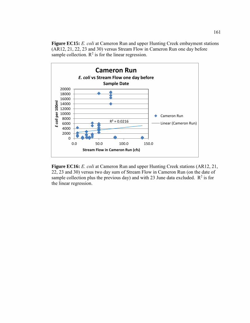
161

Figure EC15: E. coli at Cameron Run and upper Hunting Creek embayment stations (AR12, 21, 22, 23 and 30) versus Stream Flow in Cameron Run one day before sample collection. R2 is for the linear regression.

Figure EC16: E. coli at Cameron Run and upper Hunting Creek stations (AR12, 21, 22, 23 and 30) versus two day sum of Stream Flow in Cameron Run (on the date of sample collection plus the previous day) and with 23 June data excluded. R2 is for the linear regression.

R² = 0.0216

02000400060008000

100001200014000160001800020000

0.0 50.0 100.0 150.0

E co

li p

er

10

0m

l


Cameron Run E. coli vs Stream Flow one day before

Sample Date

Cameron Run

Linear (Cameron Run)

162

In reviewing the stream flow data we noted several occasions when there were high stream flow a few day before sample collection. We explored the relationship between E. coli and the sum of four days of stream flow – the four days before sample collection (Figure EC17). Again this assessment did not reveal any specific relationship between bacterial abundance and stream flow. However, when fitting a polynomial model (second power) to the data a low but significant R2 was found. More complex polynomial curves (third and fourth power) fit even better. However it seems unlikely that they are better predictors of E. coli abundance, but rather reflect some aspect of rainfall, runoff, stream flow and bacterial abundance. Nevertheless this result may give a hint as to what is driving variations in E. coli.

R² = 0.3805

R² = 0.0026

02000400060008000

100001200014000160001800020000

0 100 200 300

E co

li p

er

10

0m

l


Cameron Run E. coli vs Stream Flow (sum T0 - T-1)

Cameron Run

Cameron Run -23 June

Linear(Cameron Run)

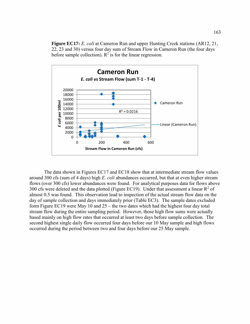
163

Figure EC17: E. coli at Cameron Run and upper Hunting Creek stations (AR12, 21, 22, 23 and 30) versus four day sum of Stream Flow in Cameron Run (the four days before sample collection). R2 is for the linear regression.

The data shown in Figures EC17 and EC18 show that at intermediate stream flow values around 300 cfs (sum of 4 days) high E. coli abundances occurred, but that at even higher stream flows (over 300 cfs) lower abundances were found. For analytical purposes data for flows above 300 cfs were deleted and the data plotted (Figure EC19). Under that assessment a linear R2 of almost 0.5 was found. This observation lead to inspection of the actual stream flow data on the day of sample collection and days immediately prior (Table EC3). The sample dates excluded form Figure EC19 were May 10 and 25 – the two dates which had the highest four day total stream flow during the entire sampling period. However, those high flow sums were actually based mainly on high flow rates that occurred at least two days before sample collection. The second highest single daily flow occurred four days before our 10 May sample and high flows occurred during the period between two and four days before our 25 May sample.

R² = 0.0216

02000400060008000

100001200014000160001800020000

0 200 400 600

E co

li p

er

10

0m

l


Cameron Run E. coli vs Stream Flow (sum T-1 - T-4)

Cameron Run

Linear (Cameron Run)

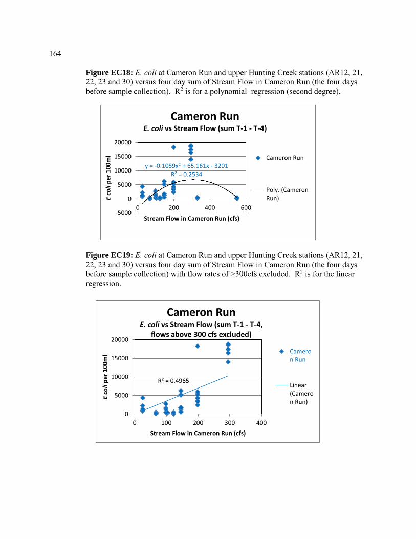
164

Figure EC18: E. coli at Cameron Run and upper Hunting Creek stations (AR12, 21, 22, 23 and 30) versus four day sum of Stream Flow in Cameron Run (the four days before sample collection). R2 is for a polynomial regression (second degree).

Figure EC19: E. coli at Cameron Run and upper Hunting Creek stations (AR12, 21, 22, 23 and 30) versus four day sum of Stream Flow in Cameron Run (the four days before sample collection) with flow rates of >300cfs excluded. R2 is for the linear regression.

y = -0.1059x2 + 65.161x - 3201R² = 0.2534

-5000

0

5000

10000

15000

20000

0 200 400 600

E co

li p

er

10

0m

l


Cameron Run E. coli vs Stream Flow (sum T-1 - T-4)

Cameron Run

Poly. (CameronRun)

R² = 0.4965

0

5000

10000

15000

20000

0 100 200 300 400

E co

li p

er

10

0m

l


Cameron Run E. coli vs Stream Flow (sum T-1 - T-4,

flows above 300 cfs excluded)

Cameron Run

Linear(Cameron Run)

165

Table EC3: Cameron Run stream flow (cfs) for the dates of sampling in 2016 and for each of the four preceding days (T-1, T-2, T-3 and T-4). The sum of the flow rates for those four days prior to sample collection is shown in the right hand column.

Sample Date

avg of 4 days

before sample T-4 T-3 T-2 T-1

Sample Date T-0

Sum T-1 - T-4

27-Apr 16.8 26 15 13 13 14 67

10-May 82.8 224 64 24 19 17 331

25-May 137.5 149 154 203 44 21 550

8-Jun 25.8 36 39 16 12 7.5 103

23-Jun 73.8 8.5 7.6 239 40 142 295.1

7-Jul 36.5 11 55 65 15 11 146

25-Jul 6.4 7.5 6.5 6.3 5.4 5.3 25.7

8-Aug 24.7 6.1 5.6 69 18 7.1 98.7

22-Aug 49.7 81 12 8.6 97 23 198.6

6-Sep 30.7 99 10 7.4 6.3 6 122.7

22-Sep 49.7 81 12 8.6 97 6.9 198.6

The data suggest the possibility that high rainfall and runoff, as indicated by higher stream flows, might wash out bacteria and result in relatively low E. coli abundance two days later if stream flows subside. The 23 June data (extreme E. coli abundances at all stations) was characterized by quite low flow three and four days prior to sample collection but very high flow two days before sample collection and also on the day of collection. It is certainly not clear that these observations could lead to predictions about E. coli abundances, but they provide a pathway for future data analysis. CONCLUSIONS

The data support a conclusion that the entire area sampled, including the mainstem of the

Potomac River (AR4) are impaired for the bacteriological water quality criterion (E. coli) content under Section 9VAC25-260-170 of the Virginia Water Quality Standards that applies to primary contact recreational use surface waters. Even the offshore Potomac River site (AR4) exceeded the 235 per 100ml criterion twice. In general more of the stations exceed the 235 per 100ml criterion in 2016 than in 2015. This was especially obvious in the latter part of the sampling period – July – Sept. In 2016 E. coli abundances >10,000 per 100ml were found at seven stations in June and one in August. In 2015 abundances above 10,000 per 100ml only occurred in two stations in May.

166

Acknowledgements Chaitanya Ravi, Monica Maricelli, and Fernanda Craig provided valuable assistance in

field sampling and lab work.

Literature Cited U.S. Environmental Protection Agency (USEPA). 2009. Method 1603: Escherichia coli (E.

coli) in Water by Membrane Filtration Using Modified membrane-Thermotolerant Escherichia coli Agar (Modified mTEC). Available at:

< http://water.epa.gov/scitech/methods/cwa/bioindicators/> search Method 1603, December 2009.

U.S. Environmental Protection Agency (USEPA). 2012. Water: Monitoring & Assessment: 5.11 Fecal Bacteria. Available at: http://water.epa.gov/type/rsl/monitoring/vms511.cfm

U.S. Environmental Protection Agency (USEPA). 2014. National Water Quality Assessment Report, water Quality Assessment and Total Maximum Daily Loads Information. Available at: <http://ofmpub.epa.gov/waters10/attains_index.control>

Virginia Department of Environmental Quality (VADEQ). 2010. Bacteria TMDLs for the Hunting Creek, Cameron Run, and Holmes Run Watersheds. Available at: <deq.state.va.us>

Virginia Department of Environmental Quality (VADEQ). 2012. 2012 Impaired Waters: Category 4 & 5 by Basin and Stream Name, Potomac and Shenandoah River Basins, Cause Group Code: A13R-03-BAC - Cameron Run/Hunting Creek. Available at: <http://www.deq.virginia.gov/Programs/Water/WaterQualityInformationTMDLs/WaterQualityAssessments.aspx>

Virginia. State Water Control Board (VSWCB). 2011. 9 VAC 25-260-10 Designation of uses. Virginia Water Quality Standards. Available at: <http://lis.virginia.gov/cgi-bin/legp604.exe?000+reg+9VAC25-260-10>

Virginia. State Water Control Board (VSWCB). 2011b. 9 VAC 25-260-170 Bacteria; other recreational waters. Virginia Water Quality Standards. Available at:

<http://lis.virginia.gov/cgi-bin/legp604.exe?000+reg+9VAC25-260-170>

http://water.epa.gov/scitech/methods/cwa/bioindicators/

http://water.epa.gov/type/rsl/monitoring/vms511.cfm

167

APPENDIX A

Figure A1: Maps of sample sites

168

Table A1: E. coli abundances, mean of triplicate analyses per sample, seasonal overall means and standard deviations and percent exceedances of criteria.

2016 AlexRenew Escherichia coli enumeration EPA Method 1603 Controls + 100ml of sterile, phosphate buffer. No E. coli-like colonies detected.

Station Sample

Date

E coli per

100ml from

100ml sample

Seasonal Mean E. coli

per 100ml

Seasonal StdDev E. coli

per 100ml

Percent Exceedences

of 126 per 100ml

Percent exceedances

of 235 per 100ml

stream flow T-1 d (cfs)

yyyymmdd

AR1 20160427 240 1965 2758 91 73 26

AR1 20160510 260 224

AR1 20160525 230 149

AR1 20160608 128 36

AR1 20160623 8600 8.5

AR1 20160707 490 11

AR1 20160725 4433 7.5

AR1 20160808 4400 6.1

AR1 20160822 557 81

AR1 20160906 78 99

AR1 20160922 2200 81

AR10 20160427 9 309 358 64 36 26

AR10 20160510 68 224

AR10 20160525 106 149

AR10 20160608 59 36

AR10 20160623 1268 8.5

AR10 20160707 230 11

AR10 20160725 150 7.5

AR10 20160808 210 6.1

AR10 20160822 533 81

AR10 20160906 340 99

AR10 20160922 430 81

AR11 20160427 55 3333 4831 91 91 26

AR11 20160510 383 224

AR11 20160525 580 149

AR11 20160608 857 36

AR11 20160623 15933 8.5

169

AR11 20160707 453 11

AR11 20160725 5533 7.5

AR11 20160808 798 6.1

AR11 20160822 5200 81

AR11 20160906 403 99

AR11 20160922 6467 81

AR12 20160427 85 3446 5454 91 82 26

AR12 20160510 383 224

AR12 20160525 193 149

AR12 20160608 247 36

AR12 20160623 18600 8.5

AR12 20160707 6233 11

AR12 20160725 2233 7.5

AR12 20160808 1600 6.1

AR12 20160822 2467 81

AR12 20160906 463 99

AR12 20160922 5400 81

AR13 20160427 350 4462 6165 100 100 26

AR13 20160510 573 224

AR13 20160525 558 149

AR13 20160608 610 36

AR13 20160623 21600 8.5

AR13 20160707 5633 11

AR13 20160725 7000 7.5

AR13 20160808 4500 6.1

AR13 20160822 4633 81

AR13 20160906 727 99

AR13 20160922 2900 81

AR2 20160427 195 336 475 64 36 26

AR2 20160510 250 224

AR2 20160525 111 149

AR2 20160608 22 36

AR2 20160623 577 8.5

AR2 20160707 1693 11

AR2 20160725 136 7.5

AR2 20160808 320 6.1

AR2 20160822 66 81

AR2 20160906 233 99

AR2 20160922 95 81

170

AR21 20160427 443 3195 5023 91 91 26

AR21 20160510 530 224

AR21 20160525 293 149

AR21 20160608 367 36

AR21 20160623 17400 8.5

AR21 20160707 1333 11

AR21 20160725 4367 7.5

AR21 20160808 2767 6.1

AR21 20160822 2433 81

AR21 20160906 41 99

AR21 20160922 5167 81

AR22 20160427 71 2635 5505 91 91 26

AR22 20160510 390 224

AR22 20160525 230 149

AR22 20160608 333 36

AR22 20160623 18800 8.5

AR22 20160707 600 11

AR22 20160725 813 7.5

AR22 20160808 420 6.1

AR22 20160822 3600 81

AR22 20160906 357 99

AR22 20160922 3367 81

AR23 20160427 120 4369 6654 91 91 26

AR23 20160510 250 224

AR23 20160525 410 149

AR23 20160608 407 36

AR23 20160623 16467 8.5

AR23 20160707 5133 11

AR23 20160725 1000 7.5

AR23 20160808 1347 6.1

AR23 20160822 18267 81

AR23 20160906 390 99

AR23 20160922 4267 81

AR3 20160427 46 642 754 55 55 26

AR3 20160510 82 224

AR3 20160525 102 149

AR3 20160608 37 36

AR3 20160623 2433 8.5

AR3 20160707 820 11

171

AR3 20160725 1332 7.5

AR3 20160808 1138 6.1

AR3 20160822 63 81

AR3 20160906 403 99

AR3 20160922 600 81

AR30 20160427 190 2820 4105 100 91 26

AR30 20160510 510 224

AR30 20160525 273 149

AR30 20160608 507 36

AR30 20160623 14000 8.5

AR30 20160707 1740 11

AR30 20160725 1310 7.5

AR30 20160808 2700 6.1

AR30 20160822 3400 81

AR30 20160906 420 99

AR30 20160922 5967 81

AR4 20160427 23 256 420 27 18 26

AR4 20160510 78 224

AR4 20160525 100 149

AR4 20160608 65 36

AR4 20160623 1407 8.5

AR4 20160707 23 11

AR4 20160725 123 7.5

AR4 20160808 203 6.1

AR4 20160822 77 81

AR4 20160906 643 99

AR4 20160922 69 81

173

Micropollutants in Alluvial Sediments and Water from Hunting Creek

2016

Thomas B. Huff, Gregory D. Foster, Zeima Kassahun, and Tabitha King The Shared Research Instrumentation Facility

And Potomac Environmental Research and Education Center

George Mason University Fairfax, VA 22030

Final Report

20 March 2017

174

Introduction

Pollutants of greatest concern in the Chesapeake Bay watershed include legacy chemicals such as polycyclic aromatic hydrocarbons (PAHs), pesticides, polychlorinated biphenyls (PCBs) and emerging pollutants such as pharmaceuticals, personal care products and endocrine disrupting chemicals (EDCs). The pollutants’ path into the aquatic environment through industrial waste discharge, urban stormwater runoff and wastewater treatments plants should be studied and analyzed further in light of emerging evidence proving EDCs in the environment pose a serious health threat 1. Sediment and water collected from Hunting Creek (northern Virginia, USA) in 2016 (May through October) were analyzed for selected emerging micropollutants. The present study is a continuation of the 2015 collaboration between the Potomac Environmental Research and Education Center (PEREC) at George Mason University and the Alexandria Renew Enterprises. Hunting Creek is a tidal embayment formed where Cameron Run meets the tidal Potomac River in northern Virginia. Substantial in-stream concentrations of anthropogenically-derived chemicals are expected in the study are due to the dense urban development and wastewater treatment plant discharge compared to the freshwater flow in the stream 2.

Micropollutants find their way into the aquatic environment primarily through urban stormwater runoff, industrial emissions, and wastewater treatment plant discharge or releases. When released into natural waters these chemicals accumulate in organic matter and fine-grained sediments or suspended sediment particles. Because storm runoff and wastewater discharge represent a sizable fraction of the annual surface water flow in urban regions, these sources are often sufficient to promote in-stream accumulation of micropollutants. Thus, the entire aquatic community may be exposed throughout entire life cycles and across generations to mixtures of biologically-active chemicals in urban areas3 . To better understand the implications of micropollutants in the Potomac River ecosystem, further ecological baseline investigations are needed since little is known regarding the fate, effects and distribution of endocrine disrupting pollutants (EDCs) in particular, in the aquatic environment.

The 2016 effort was patterned on the long-running Gunston Cove Study which PEREC has been conducting in partnership with the County of Fairfax Department of Public Works and Environmental Services since 1984.

Study Objectives

Water and alluvial sediments collected in the vicinity of the Hunting Creek embayment of the Potomac River were analyzed for micropollutants associated with urban sources. The objectives of the present investigation include the following considerations:

175

Quantify the concentrations of micropollutants in sediments and water in the Hunting Creek region of the Potomac River.

Expand the list of target compounds from the 2015 micropollutant analysis to include additional classes of emerging contaminants using both gas chromatography-mass spectrometry and liquid chromatography coupled with triple-quadrupole mass spectrometry.

Determine the presence and concentrations of target analyte metabolites.

We report here on methods development to broaden the range of analytes being determined and provide some preliminary results. More results will be available in the final report.

Materials and Methods

Standards and Reagents:

Certified standards of target micropollutants were purchased from Sigma-Aldrich (St. Louis, MO) except for acenaphthenee-d10. phenanthrene-d10 and chrysene-d12 which were purchased from Restek Corporation (State College, PA), n-propylparaben-13C3, and ethylparaben-13C6 which were purchased from Cambridge Isotope Laboratories (Tewksbury, MA), and atrazine mercapturate which was purchased from Santa Cruz Biotechnology, Inc. (Dallas, TX). Working standards were prepared according to the groups in Tables 2 and 3 in acetonitrile and stored at -20 oC. The derivatization agent, N-Methyl-N-[(tert-butyldimethylsilyl) trifluoroacetamide (MTBSTFA) containing 1% tert-butyldimethylchlorosilane (TBDMS) was purchased from Restek in 1-mL vials. Solid phase extraction (SPE) cartridges included Strata-X 33 µm polymeric reverse-phase (200 mg/6 mL), Strata-X-C 33 µm polymeric strong cation (100 mg/6 mL), and Strata-X-A 33 µm polymeric strong anion (100 mg/6 mL) were obtained from Phenomenex (Torrance, CA). QuEChERS extraction kits included AOAC 2007.01 method roQ™ extraction tubes, roQ™ PSA dSPE sample extract cleanup kits, and roQ™ PSA/C18 dSPE sample extract kits from Phenomenex (Torrance, CA). Ethyl acetate (EtOAc), dichloromethane (DCM), methyl-tert-butyl ether (MTBE), and methanol (MeOH) were all HPLC-grade and supplied by Fisher Scientific (Hanover Park, IL). LC-MS grade acetonitrile (ACN) was purchased from Sigma-Aldrich. Ultra-high-purity water (UHP-W) was produced in house by a centralized deionized, reverse-osmosis system feeding a Thermo Scientific GenPure xCAD UV/UF + TOC point-of-use system (Fisher Scientific). Sample containers (1-L amber glass bottles for water and 300 mL clear glass jars for sediments) and all glassware used for sample and preparation are cleaned by washing with soap, rinsing with distilled water followed by double distilled water (DDW), and ashed at 450 oC overnight. All laboratory materials are made of glass, stainless steel or Teflon to avoid sample contamination. The Teflon materials are cleaned the same way as glass but without ashing. All materials both made of glass and Teflon are rinsed with methanol and air dried before use.

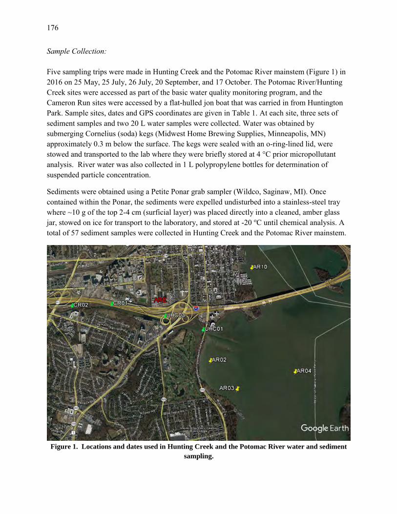
176

Sample Collection: Five sampling trips were made in Hunting Creek and the Potomac River mainstem (Figure 1) in 2016 on 25 May, 25 July, 26 July, 20 September, and 17 October. The Potomac River/Hunting Creek sites were accessed as part of the basic water quality monitoring program, and the Cameron Run sites were accessed by a flat-hulled jon boat that was carried in from Huntington Park. Sample sites, dates and GPS coordinates are given in Table 1. At each site, three sets of sediment samples and two 20 L water samples were collected. Water was obtained by submerging Cornelius (soda) kegs (Midwest Home Brewing Supplies, Minneapolis, MN) approximately 0.3 m below the surface. The kegs were sealed with an o-ring-lined lid, were stowed and transported to the lab where they were briefly stored at 4 °C prior micropollutant analysis. River water was also collected in 1 L polypropylene bottles for determination of suspended particle concentration.

Sediments were obtained using a Petite Ponar grab sampler (Wildco, Saginaw, MI). Once contained within the Ponar, the sediments were expelled undisturbed into a stainless-steel tray where ~10 g of the top 2-4 cm (surficial layer) was placed directly into a cleaned, amber glass jar, stowed on ice for transport to the laboratory, and stored at -20 oC until chemical analysis. A total of 57 sediment samples were collected in Hunting Creek and the Potomac River mainstem.

Figure 1. Locations and dates used in Hunting Creek and the Potomac River water and sediment

sampling.

177

Table 1. Details of collections sites, dates, labeling codes and GPS locations.

Date Location Labeling code GPS Coordinates

05-May-16 Potomac River AR02 38° 47.115’ N, 77° 3.108’ W AR03 38⁰ 46.813’ N, 77⁰ 2.887’ W AR04 38⁰ 46.838’ N, 77⁰ 2.184’ W AR10 38⁰ 47.855’ N, 77⁰ 2.341’ W 25-Jul-16 Potomac River AR02 38⁰ 47.120’ N, 77⁰ 2.971’ W AR03 38⁰ 46.934’ N, 77⁰ 2.939’ W AR04 38⁰ 46.838’ N, 77⁰ 2.184’ W AR10 38⁰ 47.819’ N, 77⁰ 2.354’ W 26-Jul-16 Hunting Creek UHC01 38⁰ 47.408’ N, 77⁰ 3.103’ W UHC03 38⁰ 47.617’ N, 77⁰ 3.506’ W Cameron Run CR01 38° 47.848’ N, 77° 4.096’ W CR02 38° 47.917’ N, 77° 4.562’ W 20-Sep-16 Potomac River AR02 38⁰ 47.115’ N, 77⁰ 3.108’ W AR03 38⁰ 46.813’ N, 77⁰ 2.887’ W AR04 38⁰ 46.838’ N, 77⁰ 2.184’ W AR10 38⁰ 47.855, N, 77⁰ 2.341’ W 17-Oct-16 Hunting Creek UHC01 38⁰ 47.381’ N, 77⁰ 3.131’ W UHC03 38⁰ 47.428’ N, 77⁰ 3.092’ W Cameron Run CR01 38° 47.848’ N, 77° 4.096’ W

* Sediment samples at Site AR04 was collected ~25 m west of where the water samples were collected to avoid an Asiatic clam bed.

Sample Preparation:

In the laboratory, 20-L river water samples were pressure filtered through 150 mm diameter Whatman GF/F 0.7 µm glass fiber filters to separate particles from water. Whatman GF/D 2.7 µm prefilters were used to prevent clogging of the 0.7 µm filter . The filters were held in place using a 142 mm filter-holder stand (EMD Millipore, Billerica, MA). Ultra-high purity gaseous nitrogen was fitted to the inlet ball-lock valve of the keg (Figure 2). The keg’s outlet valve was connected to the inlet port of the filter holder. The outlet of the filter holder was connected with tubing that was used to aliquot samples. Nitrogen pressure was held at 40 psi and gas flow was carefully controlled by a needle valve forcing the water through the filter set which collected suspended particles. The filtrate was aliquoted into 1 L amber glass bottles. Nine bottles of filtered water were collected from each keg and stored at 4 °C. The filter set was sealed in an aluminum pouch prior to extraction and micropollutant analysis. The exact volume in each bottle and remaining keg water were measured for total sample volume. The 1 L water samples were vacuum filtered through pre-weighed 47 mm diameter GF/D and GF/F filter sets, air dried and weighed again for determining particle mass per liter.

178

Water Sample Extraction

The micropollutants were extracted from filtered water to which surrogate standards were added (Table 4) by using two solid phase extraction (SPE) techniques. Strata-X SPE cartridges were used for Potomac Science Center (PSC) 5100 series methods (Table 2). The cartridges were conditioned with 6 mL MTBE, equilibrated with 6 mL MeOH and 6 mL UHP-W. The samples were loaded onto the cartridges using a Supelco vacuum manifold and large volume sample tubing (Sigma-Aldrich, St. Louis, MO) at a rate of 1-2 drops per second. Following extraction, the cartridges were washed with 95:5 UHPW:MeOH and eluted with 6 mL 10:90 MeOH-MTBE into 12 mL deactivated glass centrifuge tubes. Sample were concentrated by evaporation by centrivap to 1 mL and quantitatively transferred to a 12 x 32 mm deactivated amber glass autosampler vial with PTFE lined septa for instrumental analysis.

Figure 2. Water analysis flow diagram: SPE for filtered water, MAE forfiltered particles. See

Tables 2 and 3 for PSC analytical methods micropollutant lists.

A combination SPE method was used for extracting PSC 5200 and 5300 series groups (Table 3). Strata X-A and X-C cartridges were conditioned with 6 mL of MeOH and equilibrated with 6 mL of UHP water. The cartridges were stacked with X-A on top, and 1 L samples with appropriate surrogate standards (Table 4) were loaded as per above. Following extraction, the cartridges were separated and washed with 2 mL of 95:5 UHP-W:MeOH. The X-C and X-A

20L Water

Pressure Filtration

Strata-X SPEof 1 L filtered water

GC-MS Analysisw/ MtBSTFADerivatization

PSC-5130

GC-MS Qualitative Analysis

LC-MS/MS AnalysisPSC-5260PSC-5270

Combined SPEStrata XA + XC

of 1 L filtered water

LC-MS AnalysisPSC-5230PSC-5240PSC-5250

MAE of FiltersDCM:EtOAc:MeOH

(1:1:1)

SPE Cleanup

GC-MS Analysisw/ MtBSTFA Derivatization

PSC-5130

LC-MS/MS AnalysisPSC-5230PSC-5240PSC-5250PSC-5260PSC-5270

179

cartridges were eluted separately with 6 mL of 69:29:2 MeOH:EtOAc:FA and 6 mL of 67.5:27.5:5 MeOH:EtOAc:NH4. Extracts were combined, and concentrated as per above.

Sediment Sample Extraction

Micropollutants were extracted from sediment using QuEChERS (Quick-Easy-Cheap-Effective-Rugged-Safe) protocol (Phenomenex, Inc., Torrance, CA, USA). QuEChERS protocol was essentially liquid-solid extraction followed by liquid-liquid extraction followed by sample extract cleanup. The thawed wet sediment was initially centrifuged for 10 minutes at 1500 rpm (Du Pont Sorval RC-5B, New Town, CT) to dewater prior to extraction. An aliquot was reserved for determining percent water. About 1.0 g each of dewatered sediment plus the appropriate surrogate and internal standards (Table 4) were

Figure 3. Pressure filter apparatus for collecting suspended particles and aliquoting 1 L water

samples. (Image from previous study.)

placed in two 50-mL polypropylene centrifuge tube along with 10 mL of ultra-high purity water. Internal standards were added at the beginning to preserve the analyte-to-internal standard ratio prior to analyzing sample aliquots that avoid accidentally obtaining aqueous portions of the bottom phase. One tube was labeled PPCP- and one tube was labeled PPCP+. The tubes were

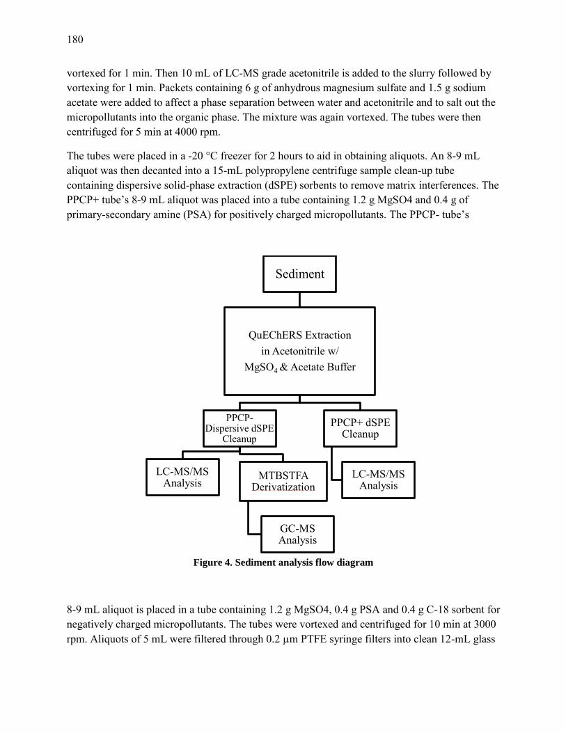
180

vortexed for 1 min. Then 10 mL of LC-MS grade acetonitrile is added to the slurry followed by vortexing for 1 min. Packets containing 6 g of anhydrous magnesium sulfate and 1.5 g sodium acetate were added to affect a phase separation between water and acetonitrile and to salt out the micropollutants into the organic phase. The mixture was again vortexed. The tubes were then centrifuged for 5 min at 4000 rpm.

The tubes were placed in a -20 °C freezer for 2 hours to aid in obtaining aliquots. An 8-9 mL aliquot was then decanted into a 15-mL polypropylene centrifuge sample clean-up tube containing dispersive solid-phase extraction (dSPE) sorbents to remove matrix interferences. The PPCP+ tube’s 8-9 mL aliquot was placed into a tube containing 1.2 g MgSO4 and 0.4 g of primary-secondary amine (PSA) for positively charged micropollutants. The PPCP- tube’s

Figure 4. Sediment analysis flow diagram

8-9 mL aliquot is placed in a tube containing 1.2 g MgSO4, 0.4 g PSA and 0.4 g C-18 sorbent for negatively charged micropollutants. The tubes were vortexed and centrifuged for 10 min at 3000 rpm. Aliquots of 5 mL were filtered through 0.2 µm PTFE syringe filters into clean 12-mL glass

Sediment

QuEChERS Extractionin Acetonitrile w/

MgSO4 & Acetate Buffer

PPCP-Dispersive dSPE

Cleanup

LC-MS/MSAnalysis

MTBSTFA Derivatization

GC-MS Analysis

PPCP+ dSPE Cleanup

LC-MS/MS Analysis

181

tubes. The volume was reduced to 1 mL in a CentriVap vacuum centrifuge and transferred to 12 x 32 mm deactivated glass autosampler vials for instrumental analysis.

Table 4. Internal and Surrogate Standards used in GCMS analysis.

Internal Standards Surrogate Standards

PSC 5100s Acenaphthene-d10 Atrazine-d5 Chrysene-d12 Bisphenol A-d16 Phenanthrene-d10 Naproxen-d3 Testosterone-13C3 Progesterone-13C3 Oxybenzone-d5 Homosalate-d4 n-Propyl Paraben-13C6 Ethyl Paraben-13C6 PSC 5200 & 5300’s Caffeine-13C3 Atrazine-d5 Ibuprofen-d3 Bisphenol A-d16 17β-Estradiol-d5 Naproxen-d3 Fluoxetine-d5 Trimethoprim-d9 Diazepam-d5 Norsertraline-13C6 Alprazolam-d5

182

Instrumental Analysis

Due to their broad range of chemical properties, target micropollutants were placed in numbered groups sharing similar properties, and instrumental analysis was performed by both LC-MS and GC-MS accordingly. Tables S1, S3, S4, and S5 in the supplemental material show the group nomenclature, the target names and the instrument used for analysis.

Liquid Chromatography-Tandem Mass Spectrometry (LC-MS-MS) Analysis

LC-MS-MS analysis was performed for less-volatile compounds using a Waters 2695 liquid chromatograph and a Quattro Micro triple quadrupole mass spectrometer with electrospray ionization (Waters Corporation, Milford, MA). The chromatographic separation was performed with either a Restek 3 µm, 2.1 x 150 mm Ultra Biphenyl HPLC column (Restek Corporation, State College, PA) or a 2.1 x 150 mm Atlantis T3 C-18aq column (Waters Corporation, Milford, MA) and a binary mobile-phase gradient with an aqueous phase of UHP-W with 0.1% FA and an organic phase of ACN with 0.1% FA. The mass spectrometer was operated in positive mode (ESI+) for compounds containing amine groups or 3-keto-4-ene cyclohexene groups and negative mode (ESI-) for compounds containing acids or phenol groups. The MS QqQ analyzer was operated in the multiple reaction monitoring (MRM) mode with quantifier and qualifier ion transitions and instrumental operating parameters determined experimentally. Individual solutions containing individual target micropollutants were infused via syringe pump through a t-type connector into the running mobile phase. The mass spectrometer MassLynx version 4.1 software then ran an autotune program that selected an abundant precursor ion and optimized the source cone voltage and then adjusted collision energy to maximize response in product ions derived from the precursor. Selected ion transition pairs provided both a quantifier and a qualifier product ion from which MRM chromatograms are formed. Supplemental Materials Tables S1, S3, S4, and S5 show the ion transition pairs for the quantifier and qualifiers as well as cone voltages and collision energies that were used. Instrumental control and data analyses were performed with Waters MassLynx and QuantLynx version 4.1 software, respectively.

GC-MS Analysis

GC-MS analyses were performed on an Agilent 7890A series gas chromatograph (Agilent Technologies, Santa Clara, CA) interfaced to an Agilent 5975C ultra-inert mass-selective detector. .Instrumental control and data analyses were performed by Agilent MSD ChemStation, version E.02.02, and Agilent MassHunter EnviroQuant version B.07 software, respectively. Instrumental configuration and operating parameters were according to the previous 2014 study with the exception that the autosampler was a customized CTC Analytics CombiPAL (Autosampler Guys, Alexandria, VA) with a refrigerated sample compartment holding the extract vials in the dark at 4 °C.

All extracts were spiked with internal standards (Table 4) prior to derivitization with N-Methyl-N-[(tert-butyldimethylsilyl) trifluoroacetamide (MTBSTFA) containing 1% tert-butyldimethylchlorosilane (TBDMS) catalyst. Prior to injection, a 100 µL aliquot of sample extract was transferred to a 300 μL vial insert amended with 50 μL of MTBSTFA and held in a heating block for 30 min at 80 oC to form tert-butyldimethyl silyl derivatives.

183

Ancillary Analysis:

The moisture content of sediment was determined gravimetrically. Sediment (~5 g) was pre-weighed, added to a porcelain thimble and heated to constant weight (~48 hrs) at 60 C. The dried sediments were reweighed to yield moisture loss. Moisture content was used to convert the wet mass of sediment determined prior to sample extraction to dry weights.

Sediment organic carbon and nitrogen contents were determined using a soil CN Analyzer. (Flash 2000, ThermoScientific, Waltham, MA). Approximately 1 g of sediment was oven dried and ground to a fine powder using mortar and pestle. The ground sample was transferred to a silver combustion cup and treated with 1 M HCl to degas carbon dioxide. Degassed sediment was redried and analyzed for C and N content using aspartic acid as the reference standard. All sediments were analyzed in triplicate.

Grain size is determined as percent sand and silty/clay using wet sieving through a 64 μm brass sieve followed by gravimetric analysis ( 0.1 mg) of the size fractions

Water Sample Results

Quality Assurance Background levels of analytes for river water sample extractions were determined by the analysis of laboratory blanks that consisted of ten replicates of 20 L UHP-W samples that were processed identically to the samples as described previously. No background levels of analytes were found in any of the laboratory blanks indicating that the glassware, filtration and extraction devices, SPE cartridges and instrument components did not contribute to any of the concentrations reported. Field blanks, which consisted of exposing 20 L of UHP-W to field conditions, also showed that none of the target micropollutant concentrations could be attributed to field contamination. All calibration curves had regression line R2 values of 0.995 or higher with a few exceptions noted in the results below. Estimated method detection limits were determined by the standard deviations of ten replicate injections of the low concentration calibration standard multiplied by the student t-test value of 3.250 (9 degrees of freedom and a confidence level of 99%). Method PSC-5230 Pharmaceuticals and Personal Care Products – ESI+ mode The Waters Corporation liquid chromatography-tandem mass spectrometer used in analyzing water samples provided two highly-specific MS2 ion transitions for each compound detected. The triple quadrupole system selects a compound-specific precursor ion at a characteristic chromatographic retention time using a predetermined cone voltage. That precursor ion is then fragmented in a collision cell to produce two compound-specific product ions created by predetermined collision energies. The tables in the Supplemental Material section lists the retention times, cone voltages, precursor ions, and collision energies used to set up the mass spectrometer method. Tables 5.1 through 5.3 show multiple reaction monitoring (MRM) chromatograms that were produced for target micropollutants found in Hunting Creek at site UHC03 on 17 October 2016.

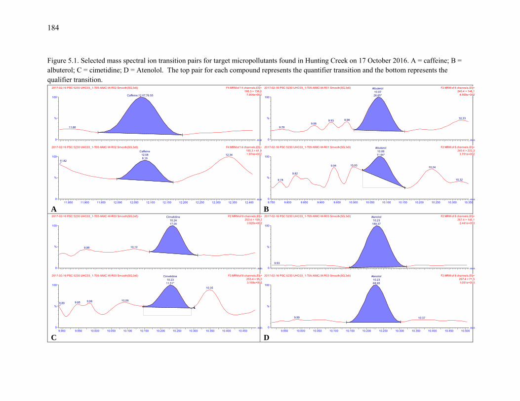
184

Figure 5.1. Selected mass spectral ion transition pairs for target micropollutants found in Hunting Creek on 17 October 2016. A = caffeine; B = albuterol; C = cimetidine; D = Atenolol. The top pair for each compound represents the quantifier transition and the bottom represents the qualifier transition.

A

B

C

D

min11.850 11.900 11.950 12.000 12.050 12.100 12.150 12.200 12.250 12.300 12.350 12.400

%

0

100

F4:MRM of 14 channels,ES+195.3 > 41.9

2017-02-16 PSC 5230 UHC03_1-T05-XAXC-W-R02 Smooth(SG,3x5)

1.974e+00212.34Caffeine

12.088.19

11.82

min

%

0

100



7.904e+002Caffeine;12.07;76.55

11.86

min9.750 9.800 9.850 9.900 9.950 10.000 10.050 10.100 10.150 10.200 10.250 10.300 10.350

%

0

100



3.751e+002

Albuterol10.0811.64*

10.009.94

9.82

9.78

10.24

10.32

min

%

0

100



4.569e+002

Albuterol10.0726.65*

9.989.939.88

9.78

10.33

min9.900 9.950 10.000 10.050 10.100 10.150 10.200 10.250 10.300 10.350 10.400 10.450

%

0

100



3.159e+002

Cimetidine10.2311.51*

10.099.989.959.89

10.35

min

%

0

100



3.920e+002

Cimetidine10.2417.04

10.129.98

min9.950 10.000 10.050 10.100 10.150 10.200 10.250 10.300 10.350 10.400 10.450 10.500

%

0

100



1.051e+003

Atenolol10.2368.95

9.99 10.37

min

%

0

100



2.441e+003

Atenolol10.23

189.37

9.93

185

Figure 5.2. Selected mass spectral ion transition pairs for target micropollutants found in Hunting Creek on 17 October 2016. A = oxycodone; B = hydrocodone; C = trimethoprim; D = triamterene. The top pair for each compound represents the quantifier transition and the bottom represents the qualifier transition.

A

B

C

D

min11.000 11.050 11.100 11.150 11.200 11.250 11.300 11.350 11.400 11.450 11.500 11.550 11.600

%

0

100



6.221e+002

Oxycodone11.3535.29

11.1811.00

min

%

0

100



1.308e+003

Oxycodone11.35

112.10

11.1211.00 11.50

min11.250 11.300 11.350 11.400 11.450 11.500 11.550 11.600 11.650 11.700 11.750 11.800

%

0

100



3.336e+002

Hydrocodone11.5917.89

11.38

11.25

11.76

min

%

0

100



4.985e+002

Hydrocodone11.5828.12

11.43

11.74

min11.400 11.450 11.500 11.550 11.600 11.650 11.700 11.750 11.800 11.850 11.900 11.950

%

-2

98



2.755e+003

Trimethoprim11.73

329.18

min

%

-0

100



2.330e+003

Trimethoprim11.73

285.16

11.50

min11.600 11.650 11.700 11.750 11.800 11.850 11.900 11.950 12.000 12.050 12.100 12.150 12.200

%

0

100



1.489e+003

Triamterene11.94

192.94

11.71

min

%

0

100



2.459e+003

Triamterene11.94

318.48

11.69

186

Figure 5.3. Selected mass spectral ion transition pairs for target micropollutants found in Hunting Creek on 17 October 2016. A = metoprolol; B = dextromethorpham; C = diphenhydramine; D = sulfamethoxazole. The top pair for each compound represents the quantifier transition and the bottom represents the qualifier transition.

A

B

C

D

min12.350 12.400 12.450 12.500 12.550 12.600 12.650 12.700 12.750 12.800 12.850 12.900

%

-1

99



1.688e+004

Metoprolol12.67

1168.18

min

%

-0

100



5.537e+003

Metoprolol12.67

374.80

min14.050 14.100 14.150 14.200 14.250 14.300 14.350 14.400 14.450 14.500

%

0

100



1.460e+003

Dextromethorphan14.28

138.03

14.11

min

%

0

100



1.512e+003

Dextromethorphan14.30

149.79

14.11

min14.250 14.300 14.350 14.400 14.450 14.500 14.550 14.600 14.650 14.700 14.750 14.800

%

0

100



1.720e+002

Diphenhydramine14.518.64

14.34

min

%

0

100



1.171e+003

Diphenhydramine14.51

124.94

14.28

min14.700 14.750 14.800 14.850 14.900 14.950 15.000 15.050 15.100 15.150 15.200 15.250

%

0

100



6.331e+003

Sulfamethoxazole14.96

474.75

min

%

0

100



9.580e+003

Sulfamethoxazole14.96

736.63

187

Surrogate recovery for the carbon 13 isotope-labeled pharmaceutical compound norsertraline-13C6 were acceptable with a mean and standard deviation (N= 53) of 70.1% ±16.1%. Carbon 13 isotope labels are more stable in water whereas deuterated compounds may dissociate a deuterium atom in aqueous solution. Selected micropollutants were spiked into duplicate samples for the 25 July 2016 trip on the Potomac. Three replicates at each site were spiked and three replicates were not spiked. The background levels of these micropollutants from the unspiked samples were subtracted from the total concentration of the spiked samples. Percent recoveries were calculated and are listed in Table 6. While the recoveries are somewhat below the acceptable levels, they are in the order of magnitude for sample concentrations. The likely cause for these results is matrix suppression of ionization in the electrospray probe of the mass spectrometer.

Table 6: Matrix spike recoveries for selected micropollutants spike

into Potomac River samples collected on 25 July 2016.

Trimethoprim 59.4% ±8.5% Caffeine 34.4% ±19.3% Sulfathiazole 32.5% ±7.6% Sulfamethazine 43.7% ±7.7% Dextromethorphan 53.1% ±10.9% Diphenhydramine 36.1% ±4.2% Sulfamethoxazole 52.9% ±11.8% Sulfaquinoxaline 67.8% ±10.1% Sulfadimethoxine 49.2% ±7.2%

The Supplemental Materials Table S2 shows the concentrations (ng/L) one standard deviations (N=3 replicates) of targeted Method PCP 5230 pharmaceutical and personal care products (PPCPs) target micropollutants found in water samples extracted by Strata XA-XC tandem solid-phase extraction cartridges and analyzed by the Waters LC-MS-MS system. Just as was the case for the 2015 study, the 2016 survey found the many of the same PPCP micropollutants including caffeine, acetaminophen, dextromethorphan and diphenhydramine. Table 7 summarizes the detection frequency, the mean concentration for the samples that had hits on a particular analyte and the maximum concentrations. The sulfonamide antibiotics sulfathiazole and sulfamethoxazole, the latter of which is most-frequently formulated with trimethoprim, were also found in many samples. Both caffeine and sulfamethoxazole were found in all samples and all replicates. Several commonly prescribed pharmaceutical compounds were added to the 2016 study. They include blood pressure medications metoprolol, atenolol, propanolol and triamterene. Two opioid pain medicines, oxycodone and hydrocodone were also added. Metoprolol was found in nearly every sample.

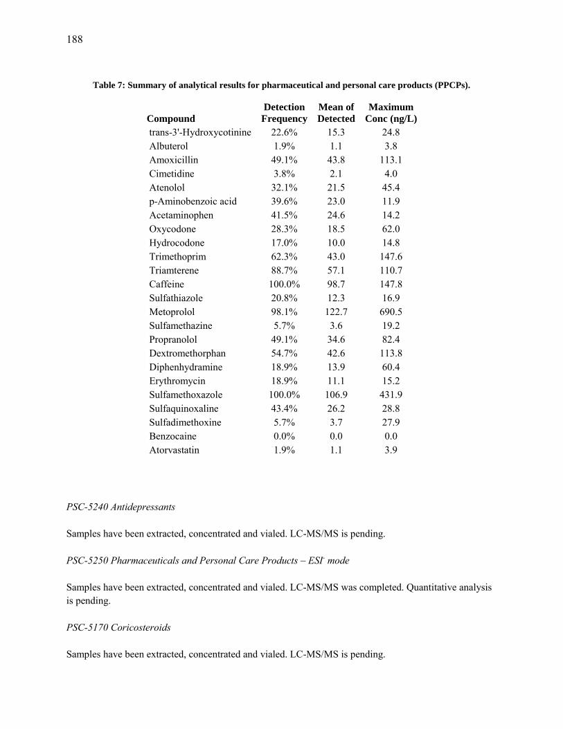
188

Table 7: Summary of analytical results for pharmaceutical and personal care products (PPCPs).

Compound

Detection

Frequency

Mean of

Detected

Maximum

Conc (ng/L)

trans-3'-Hydroxycotinine 22.6% 15.3 24.8 Albuterol 1.9% 1.1 3.8 Amoxicillin 49.1% 43.8 113.1 Cimetidine 3.8% 2.1 4.0 Atenolol 32.1% 21.5 45.4 p-Aminobenzoic acid 39.6% 23.0 11.9 Acetaminophen 41.5% 24.6 14.2 Oxycodone 28.3% 18.5 62.0 Hydrocodone 17.0% 10.0 14.8 Trimethoprim 62.3% 43.0 147.6 Triamterene 88.7% 57.1 110.7 Caffeine 100.0% 98.7 147.8 Sulfathiazole 20.8% 12.3 16.9 Metoprolol 98.1% 122.7 690.5 Sulfamethazine 5.7% 3.6 19.2 Propranolol 49.1% 34.6 82.4 Dextromethorphan 54.7% 42.6 113.8 Diphenhydramine 18.9% 13.9 60.4 Erythromycin 18.9% 11.1 15.2 Sulfamethoxazole 100.0% 106.9 431.9 Sulfaquinoxaline 43.4% 26.2 28.8 Sulfadimethoxine 5.7% 3.7 27.9 Benzocaine 0.0% 0.0 0.0 Atorvastatin 1.9% 1.1 3.9

PSC-5240 Antidepressants Samples have been extracted, concentrated and vialed. LC-MS/MS is pending. PSC-5250 Pharmaceuticals and Personal Care Products – ESI- mode Samples have been extracted, concentrated and vialed. LC-MS/MS was completed. Quantitative analysis is pending. PSC-5170 Coricosteroids Samples have been extracted, concentrated and vialed. LC-MS/MS is pending.

189

PSC-5130 Endocrine Disrupting Chemicals

Samples have been extracted, and solvent transference is being completed pending qualtitative GC-MS analysis for discovery and derivatization for GC-MS is pending.

Grad Student Work in Progress

The extraction and analysis of filtered suspended particles and sediments is being conducted by Monica Ahir for her Masters of Science degree thesis requirement in the Department of Chemistry and Biochemistry at George Mason University. Once complete, a clearer description of the partitioning of micropollutants in the aquatic ecosystem in and around Hunting Creek will emerge.

Acknowledgements

We are extremely grateful to Alexandria Renew Enterprises for providing financial support to the micropollutant study.

Appreciation is extended to Dr. Chris Jones and Laura Birsa of PEREC at George Mason University for their efforts in coordinating the collection of sediments and water which were integral to this study.

References

(1) Arnot, J. A.; Gobas, F. A. P. C. A food web bioaccumulation model for organic chemicals in aquatic ecosystems. Environmental Toxicology and Chemistry 2004, 23, 2343–2355.

(2) Crimmins, B. S.; Brown, P. D.; Kelso, D. P.; Foster, G. D. Bioaccumulation of PCBs in Aquatic Biota from a Tidal Freshwater Marsh Ecosystem. Archives of Environmental Contamination and Toxicology 2002, 42, 396–404.

(3) Nasuti, C.; Cantalamessa, F.; Daly, C. J.; McGrath, J. C. Alterations in rabbit aorta

induced by types I and II pyrethroids. Environmental Toxicology and Pharmacology 2007, 23, 250–253.

(4) Shala, L.; Foster, G. Surface Water concentrations and loading budgets of pharmaceuticals and other domestic use chemicals in an urban watershed (Washington DC). Archives of Environmental Contamination and Toxicology 2010, 58, 551-561

(5) Kawakami, T.; Isama, K.; Matsuoka, A. Analysis of phthalic acid diesters, monoester

and other plasticizers in polyvinyl chloride household products in Japan. Journal of Environmental Science and Health A 2011, 46, 855-864

190

Supplemental Material

Table S1. 2016 PSC-5230 Multiresidue Pharmaceuticals and Personal Care Products LC-MS-MS Parameters. CV = cone voltate, CE = collision energy.

MRM Group Analyte RT Precursor Product 1 CV1 CE 12 Product 2 CE 2

1 trans-3’-Hydroxycotinine 2.61 193.1 79.9 45 25 2 Albuterol 9.72 240.4 148.1 15 22 222.3 10 2 Amoxicillin 9.79 366.4 114.0 20 26 349.3 10 2 Cimetidine 9.87 253.4 95.0 20 24 159.2 16 2 Atenolol 9.88 267.4 71.5 30 26 145.1 30 3 p-Aminobenzoic acid 10.52 138.1 93.8 27 17 77.0 17 3 Acetaminophen 10.57 152.0 92.8 30 24 110.0 18 3 Oxycodone 11.05 316.4 241.2 25 36 298.3 22 3 Hydrocodone 11.30 300.4 171.1 40 46 199.2 34

4 Caffeine-13C3 IS 11.62 198.3 42.9 30 38 140.1 22 4 Caffeine 11.62 195.3 41.9 30 50 138.0 22 4 Triamterene 11.64 254.4 104.0 45 46 237.3 28 4 Trimethoprim 11.67 291.4 123.1 35 32 230.3 26 4 Oxytetracycline 11.68 461.5 426.3 20 22 443.8 16 4 Sulfathiazole 11.76 256.2 92.0 25 32 156.1 18 5 Metoprolol 12.45 268.5 71.6 30 24 74.5 24 5 Sulfamethazine 12.98 279.3 92.0 25 36 186.2 18 5 Propranolol 13.80 260.4 74.4 30 26 116.1 18 5 Trazadone 13.93 368.5 181.2 75 30 327.4 14 6 Sulfamethoxazole 14.45 254.3 92.1 25 28 156.1 18 6 Dextromethorphan 14.60 272.5 171.2 25 50 213.4 34 6 Diphenhydramine 14.75 256.5 152.1 15 44 167.2 12 7 Sulfaquinoxaline 15.43 301.4 92.2 30 34 156.2 16 7 Sulfadimethoxine 15.47 311.4 92.0 30 36 156.0 26 7 Benzocaine 15.95 166.3 76.9 25 28 138.1 16

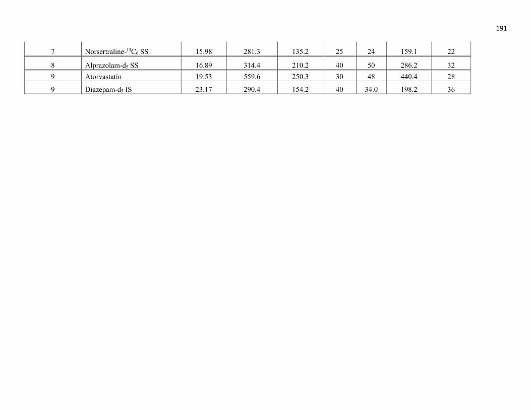
191

7 Norsertraline-13C6 SS 15.98 281.3 135.2 25 24 159.1 22

8 Alprazolam-d5 SS 16.89 314.4 210.2 40 50 286.2 32 9 Atorvastatin 19.53 559.6 250.3 30 48 440.4 28

9 Diazepam-d5 IS 23.17 290.4 154.2 40 34.0 198.2 36

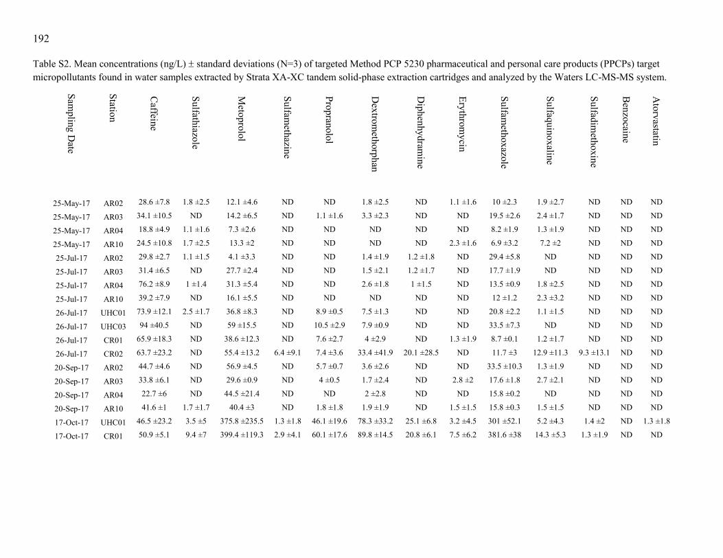
192

Table S2. Mean concentrations (ng/L) standard deviations (N=3) of targeted Method PCP 5230 pharmaceutical and personal care products (PPCPs) target micropollutants found in water samples extracted by Strata XA-XC tandem solid-phase extraction cartridges and analyzed by the Waters LC-MS-MS system.

Sampling D

ate

Station

Caffeine

Sulfathiazole

Metoprolol

Sulfamethazine

Propranolol

Dextrom

ethorphan

Diphenhydram

ine

Erythromycin

Sulfamethoxazole

Sulfaquinoxaline

Sulfadimethoxine

Benzocaine

Atorvastatin

25-May-17 AR02 28.6 ±7.8 1.8 ±2.5 12.1 ±4.6 ND ND 1.8 ±2.5 ND 1.1 ±1.6 10 ±2.3 1.9 ±2.7 ND ND ND

25-May-17 AR03 34.1 ±10.5 ND 14.2 ±6.5 ND 1.1 ±1.6 3.3 ±2.3 ND ND 19.5 ±2.6 2.4 ±1.7 ND ND ND

25-May-17 AR04 18.8 ±4.9 1.1 ±1.6 7.3 ±2.6 ND ND ND ND ND 8.2 ±1.9 1.3 ±1.9 ND ND ND

25-May-17 AR10 24.5 ±10.8 1.7 ±2.5 13.3 ±2 ND ND ND ND 2.3 ±1.6 6.9 ±3.2 7.2 ±2 ND ND ND

25-Jul-17 AR02 29.8 ±2.7 1.1 ±1.5 4.1 ±3.3 ND ND 1.4 ±1.9 1.2 ±1.8 ND 29.4 ±5.8 ND ND ND ND

25-Jul-17 AR03 31.4 ±6.5 ND 27.7 ±2.4 ND ND 1.5 ±2.1 1.2 ±1.7 ND 17.7 ±1.9 ND ND ND ND

25-Jul-17 AR04 76.2 ±8.9 1 ±1.4 31.3 ±5.4 ND ND 2.6 ±1.8 1 ±1.5 ND 13.5 ±0.9 1.8 ±2.5 ND ND ND

25-Jul-17 AR10 39.2 ±7.9 ND 16.1 ±5.5 ND ND ND ND ND 12 ±1.2 2.3 ±3.2 ND ND ND

26-Jul-17 UHC01 73.9 ±12.1 2.5 ±1.7 36.8 ±8.3 ND 8.9 ±0.5 7.5 ±1.3 ND ND 20.8 ±2.2 1.1 ±1.5 ND ND ND

26-Jul-17 UHC03 94 ±40.5 ND 59 ±15.5 ND 10.5 ±2.9 7.9 ±0.9 ND ND 33.5 ±7.3 ND ND ND ND

26-Jul-17 CR01 65.9 ±18.3 ND 38.6 ±12.3 ND 7.6 ±2.7 4 ±2.9 ND 1.3 ±1.9 8.7 ±0.1 1.2 ±1.7 ND ND ND

26-Jul-17 CR02 63.7 ±23.2 ND 55.4 ±13.2 6.4 ±9.1 7.4 ±3.6 33.4 ±41.9 20.1 ±28.5 ND 11.7 ±3 12.9 ±11.3 9.3 ±13.1 ND ND

20-Sep-17 AR02 44.7 ±4.6 ND 56.9 ±4.5 ND 5.7 ±0.7 3.6 ±2.6 ND ND 33.5 ±10.3 1.3 ±1.9 ND ND ND

20-Sep-17 AR03 33.8 ±6.1 ND 29.6 ±0.9 ND 4 ±0.5 1.7 ±2.4 ND 2.8 ±2 17.6 ±1.8 2.7 ±2.1 ND ND ND

20-Sep-17 AR04 22.7 ±6 ND 44.5 ±21.4 ND ND 2 ±2.8 ND ND 15.8 ±0.2 ND ND ND ND

20-Sep-17 AR10 41.6 ±1 1.7 ±1.7 40.4 ±3 ND 1.8 ±1.8 1.9 ±1.9 ND 1.5 ±1.5 15.8 ±0.3 1.5 ±1.5 ND ND ND

17-Oct-17 UHC01 46.5 ±23.2 3.5 ±5 375.8 ±235.5 1.3 ±1.8 46.1 ±19.6 78.3 ±33.2 25.1 ±6.8 3.2 ±4.5 301 ±52.1 5.2 ±4.3 1.4 ±2 ND 1.3 ±1.8

17-Oct-17 CR01 50.9 ±5.1 9.4 ±7 399.4 ±119.3 2.9 ±4.1 60.1 ±17.6 89.8 ±14.5 20.8 ±6.1 7.5 ±6.2 381.6 ±38 14.3 ±5.3 1.3 ±1.9 ND ND

193

Table S2. Continued.

Sampling D

ate

Station

trans-3'-Hydroxycotinine

Albuterol

Am

oxicillin

Cim

etidine

Atenolol

p-Am

inobenzoic acid

Acetam

inophen

Oxycodone

Hydrocodone

Trimethoprim

Triamterene

25-May-17 AR02 11.5 ±4.7 ND 85.9 ±21.1 ND 1.6 ±2.3 5.9 ±2.7 5.2 ±5.1 1.1 ±1.6 2.7 ±1.9 2.6 ±2 1.4 ±1.9

25-May-17 AR03 14.3 ±5.5 ND 65.9 ±29.1 ND 2.1 ±3 5.1 ±1.4 2 ±2.8 2.4 ±1.7 ND 5 ±4 7.8 ±1.4

25-May-17 AR04 20.3 ±3.9 ND 42.8 ±50.1 ND 4.7 ±1.9 1.1 ±1.6 6 ±2.2 ND 2.7 ±3.8 5.3 ±0.7 1.7 ±2.4

25-May-17 AR10 12.3 ±1.8 ND 65.3 ±17.5 ND ND 5.5 ±1.4 12.7 ±1.2 ND 1 ±1.4 1.6 ±2.3 3.3 ±2.3

25-Jul-17 AR02 ND ND 6.4 ±9.1 ND ND 5.1 ±5 1.3 ±1.8 ND 1.2 ±1.8 1 ±1.4 8.2 ±1.5

25-Jul-17 AR03 ND ND 10.2 ±6 ND ND 1.9 ±2.7 1.2 ±1.6 ND ND 1.3 ±1.8 5.8 ±0.7

25-Jul-17 AR04 ND ND ND ND ND ND ND ND ND 1.2 ±1.7 6.8 ±3

25-Jul-17 AR10 ND ND 3.8 ±5.3 ND ND 2.1 ±1.5 2.2 ±3.1 ND ND 3.1 ±2.3 5.2 ±1.5

26-Jul-17 UHC01 ND ND 4.2 ±5.9 ND ND ND 1.5 ±2.1 ND ND 5.3 ±2.4 11.1 ±4.4

26-Jul-17 UHC03 ND ND 9.3 ±8.8 ND 3.6 ±2.6 1.3 ±1.9 1.1 ±1.5 ND 1.4 ±2 10.6 ±6.3 10.6 ±3.7

26-Jul-17 CR01 ND ND 3.9 ±5.5 ND ND ND 1.1 ±1.6 1.3 ±1.8 ND 5.4 ±1.4 7 ±2.1

26-Jul-17 CR02 ND ND ND ND ND 1 ±1.5 2.5 ±1.8 3.6 ±0.3 ND 26.4 ±25 10.2 ±1.3

20-Sep-17 AR02 ND ND ND ND 3.9 ±0.5 1.4 ±2 ND ND ND 1.2 ±1.7 5.7 ±0.9

20-Sep-17 AR03 ND ND ND ND ND 1.4 ±1.9 ND ND ND 1.3 ±1.8 4.5 ±0.4

20-Sep-17 AR04 ND ND 4.1 ±3.9 ND ND ND 1.5 ±2.2 ND ND ND 3.3 ±2.5

20-Sep-17 AR10 ND ND ND ND 1.6 ±1.6 ND ND 4.1 ±0.8 ND ND 4.4 ±0.3

17-Oct-17 UHC01 ND 1.3 ±1.8 9.4 ±2.8 2.4 ±1.7 41.4 ±3.8 3.8 ±3.2 4.7 ±3.4 41.9 ±17.3 8.5 ±4.5 81 ±47.4 62.5 ±34.4

17-Oct-17 CR01 ND ND 3.1 ±4.4 ND 21.1 ±6.1 ND 2.7 ±2 9 ±1.8 ND 23.9 ±0.3 20.5 ±2.7

194

Table S3. PSC 5240 PPCP Antidepressants ESI+ LC-MS-MS Parameters. CV = cone voltate, CE = collision energy. MRM Group Analyte tR (min) Precursor Product 1 CV CE1 Product 2 CE2

1 Desmethylvenlafaxine 5.35 264.5 246.4 20 12 57.9 18 2 Venlafaxine 10.79 278.5 260.4 20 12 57.9 18 2 10,11-Carbamazepine epoxide 12.26 253.4 236.2 25 12 180.2 24 2 Citalopram 13.00 325.4 262.3 35 18 109.0 30 3 Paroxetine 13.84 330.4 192.3 30 20 69.9 32 3 Norfluoxetine 13.85 296.4 134.2 15 10 105.0 28 3 Carbamazepine 13.99 237.4 194.2 30 18 179.1 38 4 Fluoxetine-d5 IS 14.18 316.5 154.3 15 10 43.9 14 4 Fluoxetine 14.22 310.4 148.2 15 10 43.9 12 4 Nortriptyline 14.34 264.4 233.3 25 14 91.0 22 4 Oxazepam 14.37 287.4 269.2 30 14 241.2 26 4 Duloxatine 14.41 298.4 154.1 10 10 43.9 10 5 Norsertraline-13C6 SS 14.56 281.3 159.1 25 22 135.2 24 5 Norsertraline 14.57 292.4 275.2 10 12 159.8 32 5 Lorazepam 14.60 321.3 303.2 25 14 275.2 20 5 Nitrazepam 14.68 282.4 236.2 35 22 180.2 42 5 Amitriptyline 14.68 278.4 233.5 30 18 91.0 22 5 Nordiazepam 14.74 271.4 165.1 35 32 140.1 32 6 Sertraline 15.01 306.4 275.2 15 12 159.0 28 6 Clonazepam 15.35 316.3 270.2 35 24 214.2 40 6 Desmethylene Paroxetine 15.36 318.5 69.9 35 30 43.9 24 6 Alprazolam-d5 SS 15.45 314.4 286.2 40 32 210.2 50 6 Alprazolam 15.50 309.4 281.3 40 30 205.1 48 7 Temazepam 16.02 301.4 283.3 20 14 255.2 20 7 Flunitrazepam 16.40 314.4 268.3 40 30 239.3 36 7 Diazepam-d5 IS 16.83 290.4 198.2 40 36 154.2 34 7 Diazepam 16.92 285.4 257.2 35 16 154.1 30

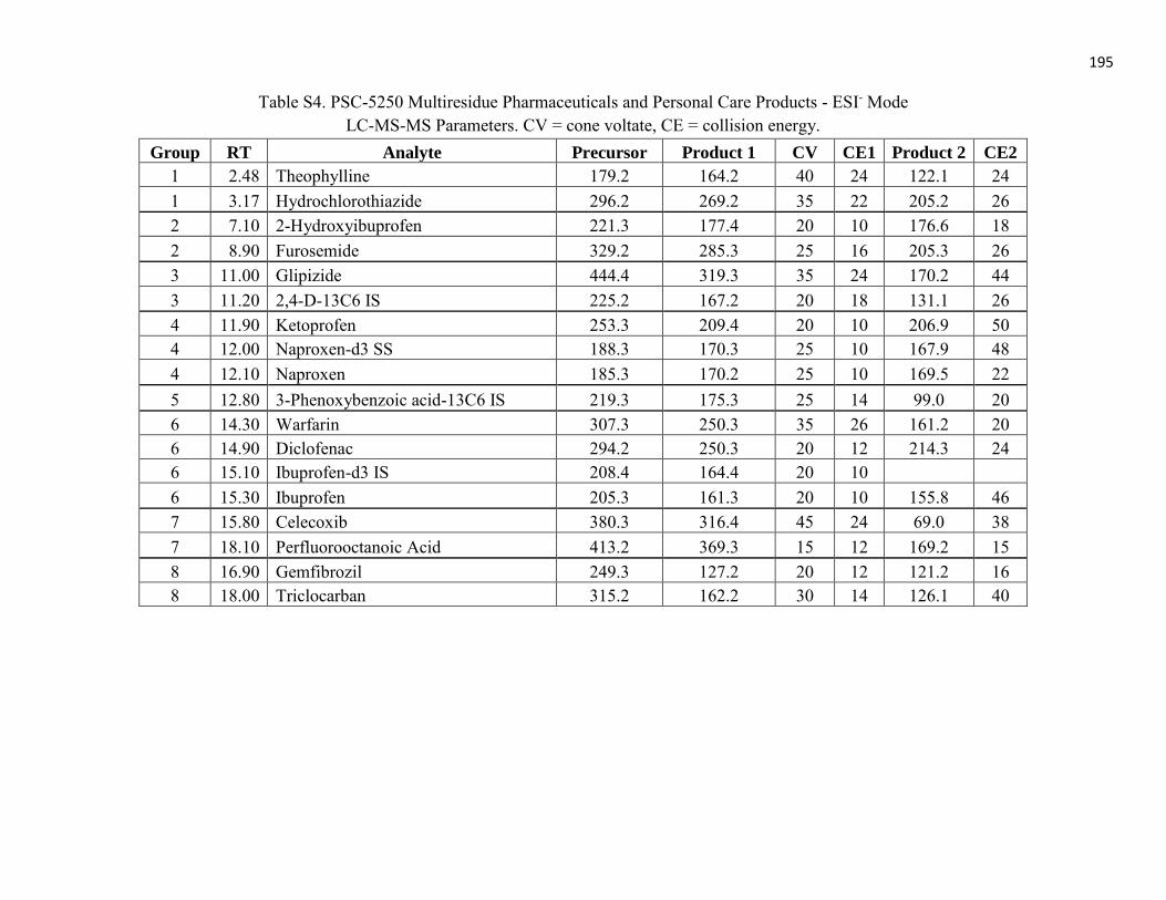
195

Table S4. PSC-5250 Multiresidue Pharmaceuticals and Personal Care Products - ESI- Mode LC-MS-MS Parameters. CV = cone voltate, CE = collision energy.

Group RT Analyte Precursor Product 1 CV CE1 Product 2 CE2

1 2.48 Theophylline 179.2 164.2 40 24 122.1 24 1 3.17 Hydrochlorothiazide 296.2 269.2 35 22 205.2 26 2 7.10 2-Hydroxyibuprofen 221.3 177.4 20 10 176.6 18 2 8.90 Furosemide 329.2 285.3 25 16 205.3 26 3 11.00 Glipizide 444.4 319.3 35 24 170.2 44 3 11.20 2,4-D-13C6 IS 225.2 167.2 20 18 131.1 26 4 11.90 Ketoprofen 253.3 209.4 20 10 206.9 50 4 12.00 Naproxen-d3 SS 188.3 170.3 25 10 167.9 48 4 12.10 Naproxen 185.3 170.2 25 10 169.5 22 5 12.80 3-Phenoxybenzoic acid-13C6 IS 219.3 175.3 25 14 99.0 20 6 14.30 Warfarin 307.3 250.3 35 26 161.2 20 6 14.90 Diclofenac 294.2 250.3 20 12 214.3 24 6 15.10 Ibuprofen-d3 IS 208.4 164.4 20 10 6 15.30 Ibuprofen 205.3 161.3 20 10 155.8 46 7 15.80 Celecoxib 380.3 316.4 45 24 69.0 38 7 18.10 Perfluorooctanoic Acid 413.2 369.3 15 12 169.2 15 8 16.90 Gemfibrozil 249.3 127.2 20 12 121.2 16 8 18.00 Triclocarban 315.2 162.2 30 14 126.1 40

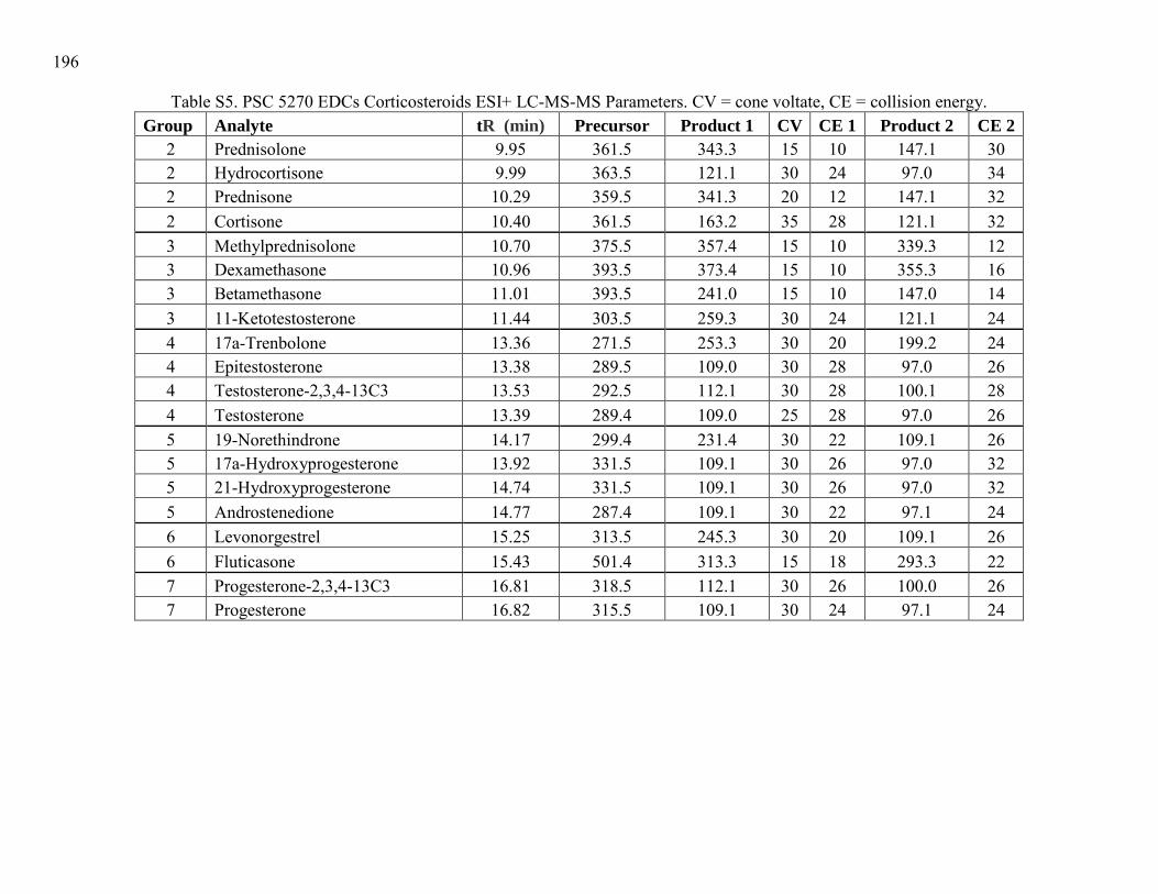
196

Table S5. PSC 5270 EDCs Corticosteroids ESI+ LC-MS-MS Parameters. CV = cone voltate, CE = collision energy. Group Analyte tR (min) Precursor Product 1 CV CE 1 Product 2 CE 2

2 Prednisolone 9.95 361.5 343.3 15 10 147.1 30 2 Hydrocortisone 9.99 363.5 121.1 30 24 97.0 34 2 Prednisone 10.29 359.5 341.3 20 12 147.1 32 2 Cortisone 10.40 361.5 163.2 35 28 121.1 32 3 Methylprednisolone 10.70 375.5 357.4 15 10 339.3 12 3 Dexamethasone 10.96 393.5 373.4 15 10 355.3 16 3 Betamethasone 11.01 393.5 241.0 15 10 147.0 14 3 11-Ketotestosterone 11.44 303.5 259.3 30 24 121.1 24 4 17a-Trenbolone 13.36 271.5 253.3 30 20 199.2 24 4 Epitestosterone 13.38 289.5 109.0 30 28 97.0 26 4 Testosterone-2,3,4-13C3 13.53 292.5 112.1 30 28 100.1 28 4 Testosterone 13.39 289.4 109.0 25 28 97.0 26 5 19-Norethindrone 14.17 299.4 231.4 30 22 109.1 26 5 17a-Hydroxyprogesterone 13.92 331.5 109.1 30 26 97.0 32 5 21-Hydroxyprogesterone 14.74 331.5 109.1 30 26 97.0 32 5 Androstenedione 14.77 287.4 109.1 30 22 97.1 24 6 Levonorgestrel 15.25 313.5 245.3 30 20 109.1 26 6 Fluticasone 15.43 501.4 313.3 15 18 293.3 22 7 Progesterone-2,3,4-13C3 16.81 318.5 112.1 30 26 100.0 26 7 Progesterone 16.82 315.5 109.1 30 24 97.1 24

197


198


199

Micropollutant Survey of Hunting Creek: Summary of Micropollutants in Water, Sediments and Fish

Gregory D Foster1 and Thomas B Huff2

1Department of Chemistry & Biochemistry, George Mason University, Fairfax, VA 22030 2Shared Research Instrumentation Facility, George Mason University, Manassas, VA, Introduction Micropollutants such as pharmaceutical chemicals, steroids and xenoestrogens have been frequently detected in surface waters over the past two decades, and the body of evidence has shown that measured concentrations are in the parts-per-trillion (ng/L) range in most cases.[1,2] The emission of micropollutants in urban centers is extensive and widespread, and as such this class of chemicals is primary concern to human and environmental health.[3] WTP discharge is becoming an increasing component of surface water runoff in urban centers. As an example, metropolitan Washington, DC maintains 37 WTPs, of which 18 are rated as high discharge capacity facilities (i.e., >7,500 m3 per day).[4] Most WTPs in metropolitan Washington, DC discharge directly into the Potomac River or adjoining tributaries, and many other WTPs outside of the DC metro region also discharge into the Potomac River. Withdrawal of the Potomac River water for public and domestic water supply, power plant cooling, industrial use and agriculture is estimated to be ~20% of the total flow.[5] Such a large degree of diversion alters the surface water chemistry and composition through the introduction of micropollutants. The toxicological implication of micropollutants in surface waters is largely unknown since very few of these chemicals are regulated, but fish reproductive abnormalities in rivers have been correlated with chemicals in WTP effluent,[6-8] including the Potomac River.[9]

The upstream tidal freshwater region of the Potomac River lies near the urban center of metropolitan Washington, DC. In this stretch of the Potomac River, the mainstem river channel expands into embayments, regions where the tidal tributaries widen into coves or small bays upon convergence with the mainstem river. These shoreline shoals and flats support submerged aquatic vegetation that provide abundant habitat for fish.[10] The embayments often occur a short distance downstream of the tributary fall-lines and are positioned in the most densely populated regions of the Potomac River watershed. An ongoing ecological field study in the Hunting Creek embayment, Alexandria (Virginia, USA) has been tasked with identifying the potential ecological impacts of wastewater treatment in the tidal freshwater Potomac River.[11] The goal of the ecological survey with respect to micropollutants has been to (i) identify potential spatial or source gradients and (ii) characterize occurrence in water, sediments and selected fish species in the vicinity of WTP discharge, such as Hunting Creek, (iii) compare the nature and concentrations of micropollutants in Hunting Creek to other regions of the Potomac River, and (iv) continue to develop, broaden and refine analytical methods to detect a greater number of chemicals for more comprehensive characterization. One of the most urgent goals is to introduce LC-MS/MS into the analytical arsenal since this instrumental technique is the industry standard in environmental analysis.

200

Matrix of Micropollutant Study in Hunting Creek Performed to Date

Year Matrices Sampleda Micropollutants Analyzed Method

2013 sediment & fish (15) water, sediment & fish (15)

PCBs (117 Congeners) PCSX (30 constituents)

GC-MS GC-MS

2014 water and sediment (27) fish (15)

PCSX (30 constituents) PCSX (dissertation research)

GC-MS GC-MS

2015 water (20) sediment (16)

PCSX (100 constituents) PCSX (30 constituents)

LC-MS GC-MS

2016 water (20) sediment (20, in progress)

PCSX (100 constituents) PCSX (50 constituents)

LC-MS/MS LC-MS/MS

aNumber of collected samples in parenthesis. PCSX = a mixture of pharmaceutical chemicals, steroids and xenoestrogens. Several micropollutant instrument schedules (chemical lists) are employed depending on the method of analysis. GC-MS = gas chromatography-mass spectrometry LC-MS = liquid chromatography-mass spectrometry LC-MS/MS = liquid chromatography-tandem mass spectrometry Summary of 2014 Results The goals of the 2014 study were to analyze water, sediments and fish from Hunting Creek for micropollutants to (i) establish a baseline of micropollutant concentrations in Hunting Creek in these matrices, (ii) identify any gradients or trajectories that could be related to the Alex WTP as a course, and (iii) characterize the distribution behavior of micropollutants between water, sediments and fish. A total of 30 micropollutants were analyzed in the samples collected in 2014 from

Hunting Creek as part of an ongoing ecological survey. The chemicals included in statistical analysis include those with an overall detection frequency of ≥50%. In water samples, 16 of the micropollutants were above 50% detection frequency in at least one of the four Hunting Creek sampling zones (Fig. 1). The largest concentrations in water were observed (in descending order) for 17-ethinylestradiol, norethindrone, mestranol and trimethoprim, with mean peak concentrations ranging from 450 (17-

Figure 1. Micropollutant concentrations in water. Mean

concentrations (+ 1 standard deviation) are provided for 2014

sampling in Cameron Run, Upper Hunting Creek, Lower Hunting

Creek and the Potomac River (reference site).

201

ethinylestradiol in lower Hunting Cr.) to 99 ng/L (testosterone in upper Hunting Cr.). The most commonly occurring micropollutants found above the detection frequency threshold in each of the four Hunting Creek sampling zones included atrazine, dextromethorphan, trimethoprim, testosterone, mestranol, norethindrone, norgestrel, 17-ethinylestradiol and estriol. The steroids as a chemical class were routinely observed. Both carbamazepine and gemfibrozil were also recurrently detected, but at relatively lower concentrations. Other minor micropollutants found in a least one of the sampling regions included 4-nonylphenol, triclosan, bisphenol A, diclofenac and progesterone. Many of the chemicals detected in Hunting Creek have been found in surface and WTP effluent discharge waters across the United States, [12-14] and it is clear that the assemblages of chemicals and their concentrations vary widely according to location. Micropollutant occurrence in surface waters is dependent on watershed population demographics, land use, WTP capacity and treatment technology, season, hydrology and aquatic geochemistry. Furthermore, it is often simply assumed that WTPs are indeed primary sources of Micropollutants in rivers and streams. It has been previously demonstrated in a small urban watershed that WTP effluent is not prerequisite for the detection of Micropollutants in stream water.[15] Further insight on sources would be extremely helpful in this regard. There were no geospatial gradients or trajectories that would pinpoint Alexandria Renew WTP as a primary source in Hunting Creek. It was apparent that upstream concentrations of the micropollutants in Cameron Run were significant for many of the chemicals. There were several examples where the upstream or downstream end-members represented the largest relative contribution of particular micropollutant concentrations in Hunting Creek, such as mestranol and norethindrone (Cameron Run) and 17-ethinylestradiol

and trimethoprim (Potomac River). The Blue Plains WTP, which is the largest WTP in the Washington, DC metropolitan region, discharges into the Potomac River 3 km upstream of Hunting Creek, and undoubtedly influences micropollutant concentrations in the mainstem Potomac River and its embayments. A total of 14 micropollutants were quantified in Hunting Creek sediments (Fig. 2).

Figure 2. Micropollutant concentrations in sediments. Mean

concentrations (+ 1 standard deviation) are provided for 2014 sampling in

Cameron Run, Upper Hunting Creek, Lower Hunting Creek and the

Potomac River (reference site).

202

The greatest concentrations were observed in lower Hunting Creek sediments for progesterone, 17-ethinylestradiol, 19-norethindrone, triclosan, acetaminophen, dextromethorphan and bisphenol A, with peak concentrations ranging from 253 to 44 ng/g dwt among these chemicals. In only one case was the largest relative concentration among the four zones found in the upstream end-member, which was escitalopram in Cameron Run sediments (16 ng/g dwt). A similar end-member maximum was observed for acetaminophen in Potomac River sediments (53 ng/g dwt). Seven Micropollutants were found in sediments from all four of the sampling zones of Hunting Creek, including 4-tert-octylphenol, atrazine, diphenhydramine, triclosan, dextromethorphan, bisphenol A, and escitalopram. The only example where WTP emissions could be correlated with sediment concentrations via spatial distribution was with progesterone, where the upstream (Cameron Run) and reference (Potomac River) concentrations were significantly less (ANOVA, p<0.05) than that observed in lower Hunting Creek (Fig. 3). Although caution in this conclusion must be emphasized because the upstream sediments had a much larger grain size and lower %TOC than lower Hunting Creek, which would influence sediment variability especially for lipophilic chemicals such as steroid hormones. As was the case with water, the steroids as a class were present at the greatest concentrations in sediments. There were 19 Micropollutants identified in banded killifish and 16 in white perch from Hunting Creek (Fig. 3), with 12 common in both species. Fish showed a moderate degree of exposure to the Micropollutants through bioaccumulation. The greatest concentrations were observed for progesterone, dextromethorphan, estrone (killifish only), bisphenol A and escitalopram. Progesterone is an endogenous human steroid and therapeutic progestogen sex hormone that is administered for birth control and to maintain hormone balance. In fish toxicology, exposure to exogenous progesterone at 63 ng/L was shown to elevate endogenous estrone in zebra fish.[16] Progesterone and estrone were both observed in banded killifish, but not

white perch, in Hunting Creek, thus, suggesting a potentially significant exposure of killifish to progesterone. Alternatively, significantly greater progesterone concentrations in adult killifish comparing the relative concentrations of the 3 chemicals among sediments and fish (Figs. 2 and 3). (Student’s-t, p<0.05) along

0

100

200

300

400

500

600

700

800

900

1000

1100

1200

1300

Ibup

rofe

nA

ceta

min

ophe

n4-

tert-

Oct

ylph

enol

Atra

zine

Caf

fein

eFl

uoxe

tine

Dip

henh

ydra

min

eV

incl

ozol

in4-

Non

ylph

enol

Gem

fibro

zil

Nap

roxe

nTr

iclo

san

Dex

trom

etho

rpha

nB

isphe

nol A

Car

bam

azap

ine

Dic

lofe

nac

Die

thyl

stilb

estro

lEs

cita

lopr

amTr

imet

hopr

imEs

trone

Equi

linEs

tradi

olTe

stoste

rone

Mes

trano

lN

oret

hind

rone

Nor

gestr

elEt

hiny

lestr

adio

lPr

oges

tero

neEs

triol

Wh

ole

Bo

dy C

on

cen

tra

tion

, n

g/g

ww

t

White PerchBanded Killifish

Figure 3. Micropollutant concentrations in white perch and killifish for

2014 sampling in Lower Hunting Creek.

203

with estrone may be linked to sexual maturation, which is a life cycle distinction relative to juvenile white perch. Dextromethorphan and bisphenol A were both enriched in fish relative to triclosan. Summary of 2015 Results The goals of the 2015 study were to (i) expand the number of micropollutants analyzed in water and sediments for better characterization, (ii) introduce LC-MS analysis of water samples to achieve an expanded list of micropollutants, (iii) continue the baseline characterization of micropollutants in water and sediments, and (iv) broaden our understanding of the distribution behavior of micropollutants in water and sediments. In the 2015 study, the analytical methods were upgraded to include a greatly expanded number of micropollutants. It has been estimated that there are >5,000 unique chemicals that fall under the classification of emerging micropollutants that may be discharged by WTP. One of the guiding objectives of our work is to develop new methods to detect and measure as many emerging micropollutants as possible, especially those which may pose the greatest risk to ecological and public health. LC-MS methods replaced many of the GC-MS methods in water analysis. LC-MS does not require chemical derivatization of the analytes prior to chemical analysis as does GC-MS. Further, many micropollutants are subject to thermal degradation via GC-MS that is not a factor in LC-MS. A total of 40 micropollutants were detected in water samples obtained from Hunting Creek (Fig. 4). The LC-MS method was successful in expanding the number of detected chemicals in water. The greatest concentrations in water were observed for sulfamethoxazole, naproxen, diclofenac, clonazepam, carbamazepine, paroxetine, norfluoxetine, duloxetine, bisphenol A, and prednisone, ranging from 700 to 50 ng/L. Geospatial correlations and trajectories with the Alex WTP were observed for a few of the chemicals, including sulfamethoxazone, paroxetine and prednisone, but for most of the micropollutants no geospatial gradients or trajectories were evident. Sediment analysis in 2015 continued with 13 of the original 30 micropollutants on the GC-MS analysis list included in the 2014 study. Because much less is known regarding micropollutants in sediments, the sediment aspect of the Hunting Creek study has been managed as a research thrust. Sediment analysis is being handled through Chemistry Master’s thesis projects. As a result, sediment methods development lags somewhat behind water analysis as water methods are tested and validated, and new chemicals of interest are identified. The MS student paired down the original list of 30 based on what was detected previously in 2014 and some analytical difficulties experienced with various analytes (poor derivatization efficiency, inconsistent calibration behavior (R2<0.90 in calibration curves), and low method recoveries), which prompted removal of chemicals from the list. Sediment is a much more complex matrix than water. Because further methods development is needed prior to switching to LC-MS for sediments, GC-MS is still used in the sediment analysis of micropollutants. The mean concentrations of the micropollutants detected in sediments in the 2015 study are shown in Fig. 5. As in 2014, the steroids were the most frequently detected and abundant micropollutants. The greatest concentrations observed were in excess of 4,000 ng/g dwt for mestranol and ethinylestradiol, and over 2,000 ng/g dwt for coprostanol. Other frequently detected micropollutants included bisphenol A, methyl triclosan, and vinclozolin. The least frequently detected micropollutants were nonylphenol, octylphenol and triclosan. The natural

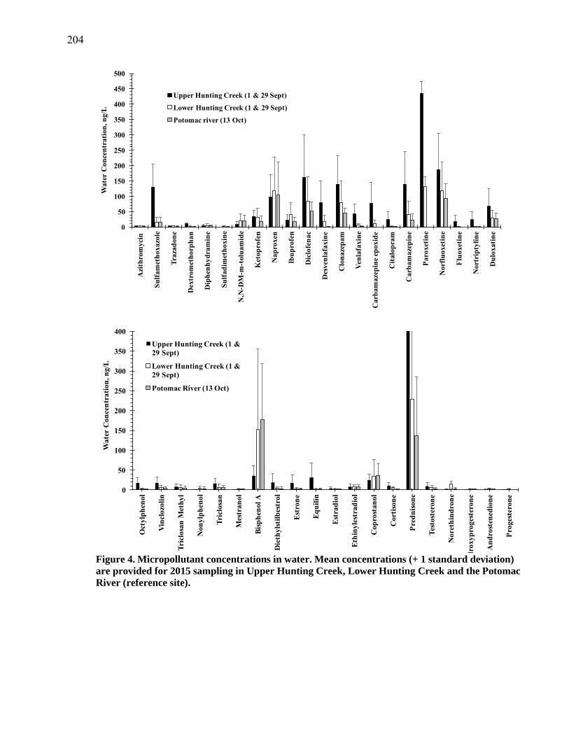
204

0

50

100

150

200

250

300

350

400

450

500

Azi

thro

my

cin

Su

lfam

eth

ox

azo

le

Tra

zad

on

e

Dex

tro

met

horp

ha

n

Dip

hen

hy

dra

min

e

Su

lfad

imet

ho

xin

e

N,N

-DM

-m-t

olu

am

ide

Ket

op

rofe

n

Nap

roxen

Ibu

pro

fen

Dic

lofe

nac

Des

ven

lafa

xin

e

Clo

na

zep

am

Ven

lafa

xin

e

Carb

am

aze

pin

e ep

ox

ide

Cit

alo

pra

m

Ca

rbam

aze

pin

e

Pa

roxet

ine

Norf

luo

xet

ine

Flu

ox

etin

e

No

rtri

pty

lin

e

Du

lox

ati

ne

Wa

ter

Co

nce

ntr

ati

on

, n

g/L

Upper Hunting Creek (1 & 29 Sept)

Lower Hunting Creek (1 & 29 Sept)

Potomac river (13 Oct)

0

50

100

150

200

250

300

350

400

Oct

ylp

hen

ol

Vin

clozo

lin

Tri

clo

san

Met

hyl

No

ny

lph

eno

l

Tri

closa

n

Mes

tra

no

l

Bis

ph

eno

l A

Die

thy

lsti

lbes

tro

l

Est

ron

e

Eq

uil

in

Est

rad

iol

Eth

inyle

stra

dio

l

Co

pro

sta

nol

Cort

ison

e

Pre

dn

iso

ne

Tes

tost

eron

e

No

reth

ind

ron

e

Hy

dro

xyp

rog

este

ron

e

An

dro

sten

edio

ne

Pro

ges

tero

ne

Wa

ter

Co

nce

ntr

ati

on

, n

g/L

Upper Hunting Creek (1 &

29 Sept)

Lower Hunting Creek (1 &

29 Sept)

Potomac River (13 Oct)

Figure 4. Micropollutant concentrations in water. Mean concentrations (+ 1 standard deviation)

are provided for 2015 sampling in Upper Hunting Creek, Lower Hunting Creek and the Potomac

River (reference site).

205

estrogens, estradiol and estrone, were found at much lower concentrations that the synthetic estrogens, EE2 and mestranol, used in human birth control and hormone replacement therapy. Coprostanol is a reduction-pathway derivative of cholesterol formed by gut microbes in the human digestive tract, and is considered a sewage marker steroid. Other xenoestrogens

(bisphenol A, nonyl- and octylphenol, and methyl triclosan) were present at much lower concentrations in sediments than the steroids.

Conclusions Micropollutants have been detected in water, sediments and fish at nanogram to microgram

per gram (or liter) concentrations. The most abundant micropollutants are the synthetic steroids (mestranol and ethinylestradiol)

and the sewage marker coprostanol. The signatures and occurrence of individual micropollutants differ across the matrices. Micropollutants tend to be present at higher concentrations in fish relative to sediments or

water. There is no geospatial correlation between micropollutant concentrations and WTP as a

primary source. We are continuing to replace GC-MS methods with LC-MS to allow a greater number of

micropollutants to be analyzed in water, sediments and fish. Future methods development includes replacing LC/-MS methods with LC-MS/MS methods

to achieve lower detection limits, a greater number of included analytes, and improved accuracy and precision in the chemical analysis.

Figure 5. Micropollutant concentrations in sediments. Mean

concentrations (+ 1 standard deviation) are provided for 2015 sampling in

Upper Hunting Creek, Lower Hunting Creek and the Potomac River

(reference site).

206

References

[1] Chiffre, A., Degiorgi, F., Bulete, A., Spinner, L. and Badot, P.-M. Occurrence of pharmaceuticals in WWTP effluents and their impact in a karstic rural catchment of Eastern France. Environ. Sci. Pollut. Res., 2016, 23, 25427-25441.

[2] Kaplan, S. Review: Pharmacological pollution in water. Crit. Rev. Environ. Sci. Technol., 2013, 43, 1074-1116.

[3] Schug, T.T., Johnson, A.F., Birnbaum, L.S., Colborn, T., Guillette, L.J., Crews, D.P., Collins, T., Soto, A.M., vom Saal, F.S., McLachlan, J.A., Sonnenschein, C. and Heindel, J.J. Minireview: Endocrine Disruptors: Past Lessons and Future Directions. Molecular Endocrinology, 2016, 30, 833-847.

[4] Governments, M.W.C.o. Metropolitan Washington Council of Governments; 1997. [5] Basin, I.C.o.t.P.R. [6] Lange, A., Paull, G.C., Hamilton, P.B., Iguchi, T. and Tyler, C.R. Implications of Persistent

Exposure to Treated Wastewater Effluent for Breeding in Wild Roach (Rutilus rutilus) Populations. Environmental Science & Technology, 2011, 45, 1673-1679.

[7] Niemuth, N.J. and Klaper, R.D. Emerging wastewater contaminant metformin causes intersex and reduced fecundity in fish. Chemosphere, 2015, 135, 38-45.

[8] Tetreault, G.R., Bennett, C.J., Shires, K., Knight, B., Servos, M.R. and McMaster, M.E. Intersex and reproductive impairment of wild fish exposed to multiple municipal wastewater discharges. Aquatic Toxicology, 2011, 104, 278-290.

[9] Iwanowicz, L.R., Blazer, V.S., Guy, C.P., Pinkney, A.E., Mullican, J.E. and Alvarez, D.A. Reproductive health of bass in the Potomac, USA, drainage: part 1. Exploring the effects of proximity to wastewater treatment plant discharge. Environ. Toxicol. Chem., 2009, 28, 1072-1083.

[10] Kraus, R.T. and Jones, R.C. Fish abundances in shoreline habitats and submerged aquatic vegetation in a tidal freshwater embayment of the Potomac River. Environmental Monitoring and Assessment, 2012, 184, 3341-3357.

[11] Jones, R.C., De Mutsert, K. and Huff, T.B., The Aquatic Monitoring Program for The Hunting Creek Area of The Tidal Freshwater Potomac River 2014 Report. Alexandria Renew Enterprises; Alexandria, VA; 2014.

[12] Bradley, P.M., Journey, C.A., Button, D.T., Carlisle, D.M., Clark, J.M., Mahler, B.J., Nakagaki, N., Qi, S.L., Waite, I.R. and VanMetre, P.C. Metformin and Other Pharmaceuticals Widespread in Wadeable Streams of the Southeastern United States. Environmental Science & Technology Letters, 2016.

[13] Kettler, T.A., Doran, J.W. and Gilbert, T.L. Simplified method for soil particle-size determination to accompany soil-quality analysis. Soil Science Society of America Journal, 2001, 65, 849-852.

[14] Kostich, M.S., Batt, A.L. and Lazorchak, J.M. Concentrations of prioritized pharmaceuticals in effluents from 50 large wastewater treatment plants in the US and implications for risk estimation. Environmental Pollution, 2014, 184, 354-359.

[15] Shala, L. and Foster, G.D. Surface Water Concentrations and Loading Budgets of Pharmaceuticals and Other Domestic-Use Chemicals in an Urban Watershed (Washington, DC, USA). Arch. Environ. Contam. Toxicol., 2010, 58, 551-561.

207

[16] Liang, Y.-Q., Huang, G.-Y., Liu, S.-S., Zhao, J.-L., Yang, Y.-Y., Chen, X.-W., Tian, F., Jiang, Y.-X. and Ying, G.-G. Long-term exposure to environmentally relevant concentrations of progesterone and norgestrel affects sex differentiation in zebrafish (Danio rerio). Aquatic Toxicology, 2015, 160, 172-179.

209

Micropollutants in Sediments from Hunting Creek: 2015 Samples

Gregory D. Foster,1,3 Thomas B. Huff,2,3 and Amanda Godfrey1

1Department of Chemistry and Biochemistry, George Mason University, Fairfax, VA 22030 3Shared Research Instrumentation Facility, George Mason University 2Potomac Environmental Research and Education Center (PEREC), George Mason University

20 February 2017

Introduction The Ecological Survey of Hunting Creek continued sediment sampling in 2015 with the

purpose of determining the identity, occurrence and environmental concentrations of selected

micropollutants. Organic micropollutants are known to be enriched in fluvial sediments in

relation to physical properties of the pollutants (e.g., water solubility and octanol/water partition

coefficient) and the geochemistry of the geosolids (e.g., grain size and organic matter content).

Sampling was conducted in 2015 in the Hunting Creek vicinity to provide a baseline of

micropollutant concentrations and to aid in identifying possible sources and impacts of

contaminants in the tidal freshwater Potomac River.

The embayments of the Potomac River that exist along the Virginia shoreline represent

important ecological habitats where the potential impacts of fluvial sources of micropollutants

may be the most readily observable. The embayments lie in densely populated areas, provide

high deposition zones for fluvial sediments and particles to be incorporated into the riverbed, and

support a diversity of aquatic life. An ongoing ecological field study in the Hunting Creek

embayment, Alexandria (Virginia, USA) has been tasked with identifying any potential

ecological impacts of wastewater treatment in the tidal freshwater Potomac River.[1] The goal of

the present investigation targeted micropollutant analysis with the intent of (i) characterizing the

presence of selected emerging (i.e., unregulated) micropollutants in sediments in the vicinity of

wastewater treatment plant discharge and (ii) identifying resolvable spatial distributions or

210

gradients that can be related to sources of any kind. The goal was to develop a greater ability to

predict the source and distribution of micropollutants in the tidal freshwater Potomac River.

Materials and methods Study Site

Hunting Creek is a tributary embayment of the Potomac River lying 8 km downstream of

Washington, DC, immediately south of the city of Alexandria, VA. Hunting Creek exists at the

stream confluence of Cameron Run and Hooff Run prior to discharging into the Potomac River.

The Cameron Run watershed, the largest of the two sub-sheds, is predominantly urban (95% of

landscape is developed) with an area of 114 km2, and the primary landscape is medium density

residential. Jones Point (Alexandria, VA) forms the northern boundary and Dyke Marsh (Fig. 1)

the southern boundary of Hunting Creek.[2] Alexandria Enterprises WTP is located north of the

shoreline of upper Hunting Creek,

and discharges an average of

150,000 m3 of wastewater daily.

Riverbed sediment were collected

in Hunting Creek for

micropollutant analysis.

Field Sampling

The Hunting Creek

sampling grid was divided into

three sub-regions based on the

location of the Alexandria Renew

WTP. The three sub-regions,

upper Hunting Creek (WTP

discharge zone), lower Hunting

Creek (downstream zone) and the

mainstem Potomac River.

Riverbed sediments

(N=11) from Hunting Creek and

the Potomac River were obtained

a

Hunting Creek 2015 Sampling

Sediment sampling locations

for 2015 Hunting Creek

Ecological Survey study

HuntingCreekMap.xlsx

All items

Lower

Hunting

Creek

Upper

Hunting Creek Potomac River

mainstem

WTP

Figure 1. Sampling sites in Hunting Creek for 2015 are shown by map pins for Lower Hunting Creek, Upper Hunting Creek and the mainstem Potomac River. Refer to Table 1 for letter designations.

(north)

(south)

a

b

a

c

d

e

f

g

211

by boat according to the same locations established for water sampling (Table 1). Sediments

were collected manually using a Petite Ponar grab sampler (Wildco, Saginaw, MI) tethered by

rope. Sediment obtained in the Ponar was carefully hauled into the boat to minimize disturbance

and expelled into a stainless steel tray, where approximately 10 g of the top 2-4 cm surficial layer

was removed and placed directly into a pre-cleaned amber glass jar using a stainless steel spoon.

The jar was sealed using a Teflon-lined lid and stored on ice for transportation to the laboratory,

whereupon the samples were stored at -20C until sample processing. The sediment sampling

sites are summarized in Fig. 1. Bulk property measurements of moisture and texture were

performed on sediments. Sediment moisture was determined by gravimetry upon drying to a

constant weight at 65 oC. Grain size was analyzed according to a reported wet sieving

technique.[3]

Table 1. Hunting Creek Sediment Sampling Dates and Locations.

Date Location Name DD Lat DD Long

9/1/15 Lower Hunting Creek (a) 38.7852500 77.0518000

Lower Hunting Creek (b) 38.7802167 77.0481167

Potomac River (north) 38.7975833 77.0390167

9/29/15 Lower Hunting Creek (c) 38.7853333 77.0495167

Lower Hunting Creek (d) 38.7822333 77.0489833

Potomac River (north) 38.7969833 77.0392333

Potomac River (south) 38.7806333 77.0364000

Potomac River (south) 38.7803000 77.0393833

10/13/15 Upper Hunting Creek (e) 38.7939500 77.0587000

Upper Hunting Creek (f) 38.7904667 77.0166667

Upper Hunting Creek (g) 38.7896833 77.0521833

Materials

Sodium sulfate (ACS grade) was supplied by VWR International Inc. (Bridgeport, NJ).

Florisil was purchased from J.T. Baker (Philipsburg, NJ). GCMS calibration standards for

quantitative analytes (Table 2) were acquired from AccuStandard (New Haven, VT). The

surrogate standards bisphenol A-d16 and atrazine-d5 were obtained from Cambridge Isotope

Laboratories (Tewksbury, MA). The internal injection standards (phenanthrene-d10 and

212

chrysene-d12) were acquired from C/D/N Isotopes Inc. (Quebec, Canada). Working standards

were prepared in acetonitrile while the surrogate standards are prepared in methanol. Final

dilutions of the GCMS calibration standards were made in toluene.

Table 2. Micropollutants Analyzed in Sediments.

Standards Phenanthrene-d10 (IS) Chrysene-d12 (IS) Atrazine-d5 (SS) Bisphenol-d16 (SS) Analytes 4-tert-Octylphenol Vinclozolin 4-Nonylphenol Triclosan Methyl Triclosan Mestranol Bisphenol A Diethylstilbestrol Estrone (E1) Equilin 17-Estradiol (E2) 17-Ethinylestradiol (EE2) Coprostanol IS, Internal injection standard; SS, surrogate standard.

Derivatization reagent, N-methyl-N-tert-butyldimethylsilyl-N-methyltrifluoroacetamide

(MtBSTFA), with 1% tert-butyldimethylchlorosilane, was purchased from Pierce (Rockford, IL)

in 1 mL ampoules. Ethyl acetate, dichloromethane, methanol and acetonitrile solvents were all

HPLC-grade and supplied by Fisher Scientific. Sample containers and all glassware used for

storage and sample preparation were cleaned by washing with soap, rinsing with distilled water

followed by double distilled water (DDW), and ashed at 400 oC overnight. DDW was produced

in the laboratory using a Corning Megapure quartz-element immersion still.

Sample Preparation

213

Sediment was initially thawed and centrifuged for 10 minutes at 1500 rpm (Du Pont

Sorval RC-5B, New Town, CT) to remove bulk water prior to extraction. Dewatered sediment (2

g) was weighed precisely (to the nearest 0.01 mg) and desiccated by mixing in a mortar and

pestle with 10 g of anhydrous sodium sulfate. The dry powder was spiked with 50-100 ng each

of the surrogate standards, transferred to a GreenChem (CEM, Matthews, NC) extraction vessel

and subjected to microwave assisted extraction (MAE) using 20 mL of 1:1:1

dichloromethane:ethyl acetate:methanol (DEM) for 15 min at 100 oC in a MARS-X microwave

extractor (CEM). The sediment analysis procedure is summarized in Fig. 2. Sediment extraction

was performed three times sequentially, the individual DEM extracts were combined in a 200

mL TurboVap cell, and the combined DEM extract was evaporated to 1 mL using a TurboVap

(Zymark, Hopkinton, MA) evaporator.

The DEM extracts were subjected to Florisil chromatography for cleanup. The Florisil

was packed in glass chromatography columns containing 6 g of 5% (wt/wt) water deactivated

Florisil between two layers (top and bottom) of 2 g of anhydrous sodium sulfate desiccant. The

columns were first conditioned with 50 mL of DEM solvent

(discarded) and the analytes were subsequently eluted with 75 mL

of DEM. The DEM solvent eluents were collected in a 200 mL

TurboVap tube and concentrated to 0.5 mL for gas

chromatography-mass spectrometry (GCMS) analysis. The eluent

was solvent-exchanged with acetonitrile during evaporation. The

final eluents were transferred to GCMS vials, and spiked with 50

µL of MtBSTFA. The mixture was heated in a vial heater block

for 30 minutes at 80 °C immediately prior to GCMS injections.

Quantified sediment concentrations of micropollutants were

expressed as ng/g dry weight (dwt).

GCMS Analysis

GCMS was performed using selected ion monitoring

(SIM) mode using an Agilent 7890A series gas chromatograph

(Agilent Technologies, Santa Clara, CA) interfaced to an Agilent

5975C mass-selective detector. Retention time locking, data

acquisition, processing, and instrumental control was performed

Sediment Sample

MAE

DEM Solvent

Florisil

Cleanup

MtBSTFA

GC-MS-SIM

Figure 2. Flow chart for sediment analysis.

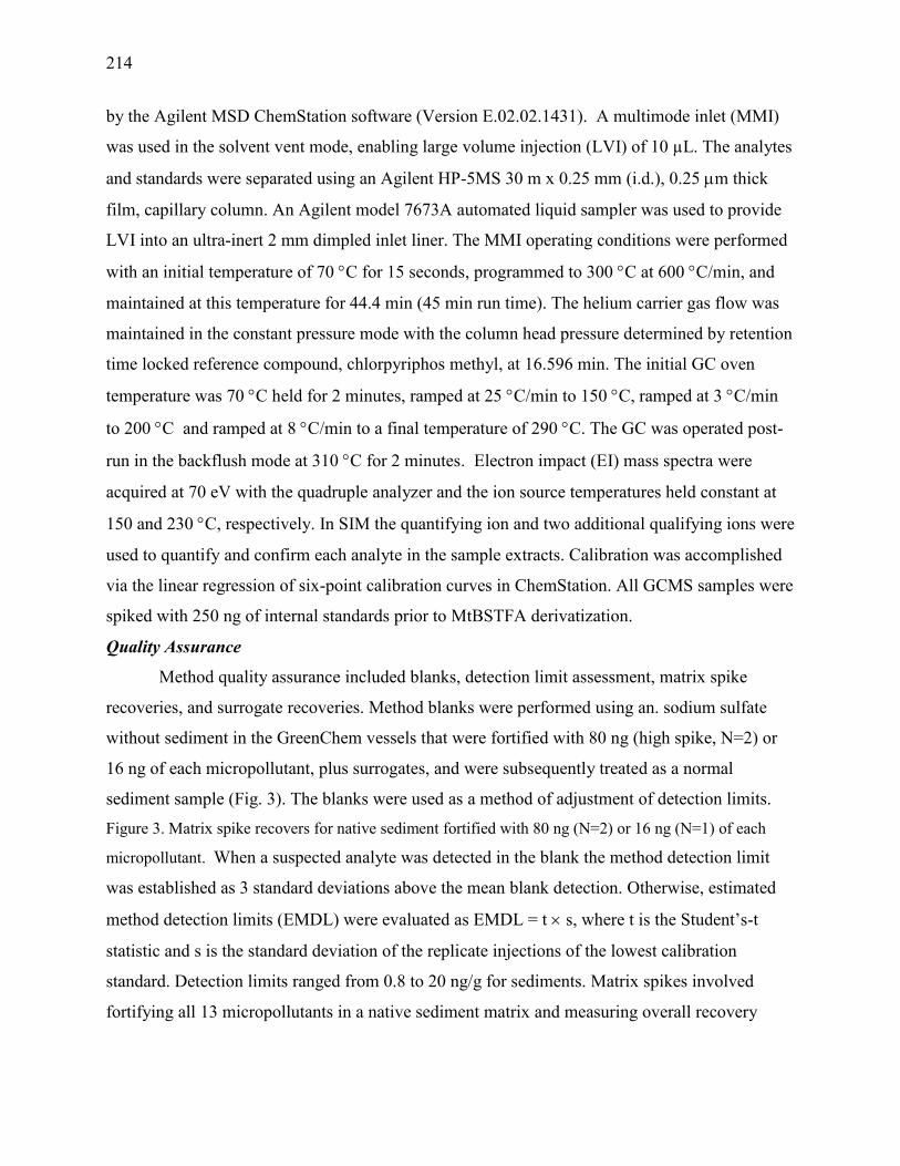
214

by the Agilent MSD ChemStation software (Version E.02.02.1431). A multimode inlet (MMI)

was used in the solvent vent mode, enabling large volume injection (LVI) of 10 µL. The analytes

and standards were separated using an Agilent HP-5MS 30 m x 0.25 mm (i.d.), 0.25 m thick

film, capillary column. An Agilent model 7673A automated liquid sampler was used to provide

LVI into an ultra-inert 2 mm dimpled inlet liner. The MMI operating conditions were performed

with an initial temperature of 70 C for 15 seconds, programmed to 300 C at 600 C/min, and

maintained at this temperature for 44.4 min (45 min run time). The helium carrier gas flow was

maintained in the constant pressure mode with the column head pressure determined by retention

time locked reference compound, chlorpyriphos methyl, at 16.596 min. The initial GC oven

temperature was 70 C held for 2 minutes, ramped at 25 C/min to 150 C, ramped at 3 C/min

to 200 C and ramped at 8 C/min to a final temperature of 290 C. The GC was operated post-

run in the backflush mode at 310 C for 2 minutes. Electron impact (EI) mass spectra were

acquired at 70 eV with the quadruple analyzer and the ion source temperatures held constant at

150 and 230 C, respectively. In SIM the quantifying ion and two additional qualifying ions were

used to quantify and confirm each analyte in the sample extracts. Calibration was accomplished

via the linear regression of six-point calibration curves in ChemStation. All GCMS samples were

spiked with 250 ng of internal standards prior to MtBSTFA derivatization.

Quality Assurance

Method quality assurance included blanks, detection limit assessment, matrix spike

recoveries, and surrogate recoveries. Method blanks were performed using an. sodium sulfate

without sediment in the GreenChem vessels that were fortified with 80 ng (high spike, N=2) or

16 ng of each micropollutant, plus surrogates, and were subsequently treated as a normal

sediment sample (Fig. 3). The blanks were used as a method of adjustment of detection limits.

Figure 3. Matrix spike recovers for native sediment fortified with 80 ng (N=2) or 16 ng (N=1) of each

micropollutant. When a suspected analyte was detected in the blank the method detection limit

was established as 3 standard deviations above the mean blank detection. Otherwise, estimated

method detection limits (EMDL) were evaluated as EMDL = t s, where t is the Student’s-t

statistic and s is the standard deviation of the replicate injections of the lowest calibration

standard. Detection limits ranged from 0.8 to 20 ng/g for sediments. Matrix spikes involved

fortifying all 13 micropollutants in a native sediment matrix and measuring overall recovery

215

through the method (Fig. 2). Matrix spike recoveries from sediment ranged from 45% (caffeine)

to 110% (bisphenol A), with a mean of 115% in the high spike and 103% in the low spike (Fig.

3). The mean surrogate recoveries in the sediment samples (± 1 standard deviation) were

6813% for bisphenol A-d16 was 8319% for atrazine-d6.

Results and Discussion The bulk sediment properties of %moisture and %silt/clay content are shown in Table 3.

Moisture was used to correct for the wet to dry weight sediment ratios for the determination of

the final sediment concentrations (ng/g dwt). Silt/clay content was completed to record sediment

grain size since it is known texture plays an important role is the sorption of micropollutants in

sediments. Sediment texture varied considerably, especially in Upper Hunting Creek where a

large percentage of sand is present. In the remaining sediments, texture varied between 55% to

95% in silt/clay content.

0

20

40

60

80

100

120

140

160

180

Oct

ylp

hen

ol

Vin

clozo

lin

Tri

clo

san

Met

hy

l

No

ny

lph

eno

l

Tri

closa

n

Mes

tran

ol

Bis

ph

enol

A

Die

thy

lsti

lbes

tro

l

Est

ron

e

Eq

uil

in

Est

rad

iol1

thy

ny

lest

rad

iol

Cop

rost

an

ol

% R

ecover

y o

f M

atr

ix S

pik

e

80 ng

16 ng

Figure 3. Matrix spike recoveries of micropollutants in native Potomac River sediment.

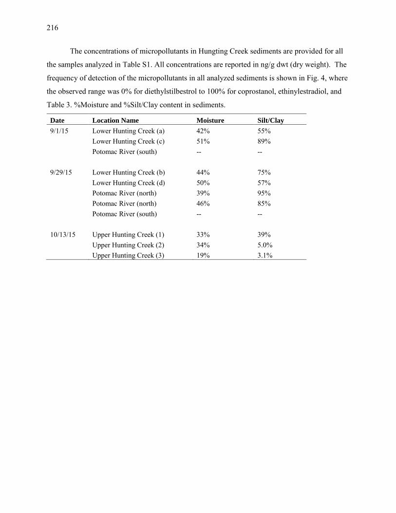
216

The concentrations of micropollutants in Hungting Creek sediments are provided for all

the samples analyzed in Table S1. All concentrations are reported in ng/g dwt (dry weight). The

frequency of detection of the micropollutants in all analyzed sediments is shown in Fig. 4, where

the observed range was 0% for diethylstilbestrol to 100% for coprostanol, ethinylestradiol, and

Table 3. %Moisture and %Silt/Clay content in sediments.

Date Location Name Moisture Silt/Clay

9/1/15 Lower Hunting Creek (a) 42% 55%

Lower Hunting Creek (c) 51% 89%

Potomac River (south) -- --

9/29/15 Lower Hunting Creek (b) 44% 75%

Lower Hunting Creek (d) 50% 57%

Potomac River (north) 39% 95%

Potomac River (north) 46% 85%

Potomac River (south) -- --

10/13/15 Upper Hunting Creek (1) 33% 39%

Upper Hunting Creek (2) 34% 5.0%

Upper Hunting Creek (3) 19% 3.1%

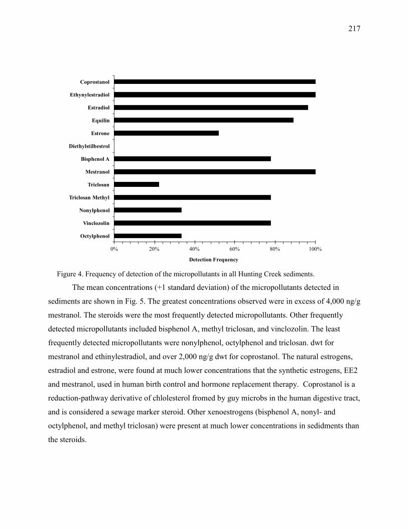
217

The mean concentrations (+1 standard deviation) of the micropollutants detected in

sediments are shown in Fig. 5. The greatest concentrations observed were in excess of 4,000 ng/g

mestranol. The steroids were the most frequently detected micropollutants. Other frequently

detected micropollutants included bisphenol A, methyl triclosan, and vinclozolin. The least

frequently detected micropollutants were nonylphenol, octylphenol and triclosan. dwt for

mestranol and ethinylestradiol, and over 2,000 ng/g dwt for coprostanol. The natural estrogens,

estradiol and estrone, were found at much lower concentrations that the synthetic estrogens, EE2

and mestranol, used in human birth control and hormone replacement therapy. Coprostanol is a

reduction-pathway derivative of chlolesterol fromed by guy microbs in the human digestive tract,

and is considered a sewage marker steroid. Other xenoestrogens (bisphenol A, nonyl- and

octylphenol, and methyl triclosan) were present at much lower concentrations in sedidments than

the steroids.

0% 20% 40% 60% 80% 100%

Octylphenol

Vinclozolin

Nonylphenol

Triclosan Methyl

Triclosan

Mestranol

Bisphenol A

Diethylstilbestrol

Estrone

Equilin

Estradiol

Ethynylestradiol

Coprostanol

Detection Frequency

Figure 4. Frequency of detection of the micropollutants in all Hunting Creek sediments.

218

Figure 5. Mean concentrations of the micropollutants in Hunting Creek sediments (+1 standard deviation).

The geospatial distribution of the micropollutants indicated there was no significant

difference among concentrations by sub-region in Hunting Creek (ANOVA, p<0.05). Upper and

Lower Hunting Creek, and Potomac River sediments all showed similar concentrations. The

apparently lower concentration of micropollutants in Upper Hunting Creek was undoubtedly

related to sediment texture (Table 3), with sand being an inert substrate for sorption and uptake

into geolsolids. Previous field studies have shown that it is more common for surfactant

chemicals to exceed steroid concentrations in water and sediments in the vicinity of WTPs.[4; 5]

The results of our study show the opposite trend. The steroid pharmaceutical chemicals found in

Hunting Creek substantially exceed the concentrations reported at other locations throughout the

world.[6; 7]

References

219

1. Jones, R.C., De Mutsert, K. and Huff, T.B. 2014 The Aquatic Monitoring Program for The Hunting Creek Area of The Tidal Freshwater Potomac River 2014 Report. Alexandria Renew Enterprises. Alexandria, VA.

2. Fairfax County Stormwater Planning Division. 2007 Cameron Run: Watershed Management Plan. http://www.fairfaxcounty.gov/dpwes/watersheds/publications/cr/ca_plan.pdf.

3. Kettler, T.A., Doran, J.W. and Gilbert, T.L. Simplified method for soil particle-size determination to accompany soil-quality analysis. Soil Sci. Soc. Am. J., 2001, 65, 849-852.

4. Langston, W.J., Burt, G.R., Chesman, B.S. and Vane, C.H. Partitioning, bioavailability and effects of oestrogens and xeno-oestrogens in the aquatic environment. J Mar Biol Assoc UK, 2005, 85, 1-31.

5. Cargouët, M., Perdiz, D., Mouatassim-Souali, A., Tamisier-Karolak, S. and Levi, Y. Assessment of river contamination by estrogenic compounds in Paris area (France). Sci. Total Environ., 2004, 324, 55-66.

6. Viganò, L., Benfenati, E., Cauwenberge, A.v., Eidem, J.K., Erratico, C., Goksøyr, A., Kloas, W., Maggioni, S., Mandich, A. and Urbatzka, R. Estrogenicity profile and estrogenic compounds determined in river sediments by chemical analysis, ELISA and yeast assays. Chemosphere, 2008, 73, 1078-1089.

7. Lei, B., Huang, S., Zhou, Y., Wang, D. and Wang, Z. Levels of six estrogens in water and sediment from three rivers in Tianjin area, China. Chemosphere, 2009, 76, 36-42.

http://www.fairfaxcounty.gov/dpwes/watersheds/publications/cr/ca_plan.pdf

220

Table S1. Concentrations of micropollutants in Hunting Creek Sediments. (Concentrations valid to 3 significant figures.)

Sample Name

2015-09-01

Lower

Hungting Cr

Site a Rep 1

2015-09-01

Lower

Hungting Cr

Site a Rep 2

2015-09-01

Lower

Hungting Cr

Site c Rep 1

2015-09-01

Lower

Hungting Cr

Site c Rep 2

2015-09-01

Lower

Hungting Cr

Site c Rep 3

2015-09-29

Lower

Hungting Cr

Site b Rep 1

2015-09-29

Lower

Hungting Cr

Site b Rep 2

2015-09-29

Lower

Hungting Cr

Site b Rep 3

2015-09-29

Lower

Hungting Cr

Site d Rep 1

2015-09-29

Lower

Hungting Cr

Site d Rep 2

2015-09-29

Lower

Hungting Cr

Site d Rep 3

Compound Name Conc. (ng/g) Conc. (ng/g) Conc. (ng/g) Conc. (ng/g) Conc. (ng/g) Conc. (ng/g) Conc. (ng/g) Conc. (ng/g) Conc. (ng/g) Conc. (ng/g) Conc. (ng/g)

Octylphenol 22.7 <16 <16 <16 <16 <16 <16 32.1 101.0 99.1 114.2

Vinclozolin 261.3 163.3 229.2 95.0 44.1 197.6 253.0 86.7 184.6 918.6 104.2

Nonylphenol 30.4 <16 <16 <16 <16 <16 21.5 38.9 55.2 75.9 113.0

Triclosan Methyl 92.5 54.1 31.5 44.7 50.2 67.7 94.5 71.4 66.3 62.1 80.0

Triclosan <16 <16 <16 <16 <16 0.0 0.0 24.4 19.5 19.0 57.6

Mestranol 4962.8 2884.8 2023.8 2063.7 511.5 2236.1 8549.9 1670.8 6629.5 9322.1 4395.0

Bisphenol A 39.3 <16 71.3 110.2 244.1 108.6 96.0 495.9 665.8 828.9 272.6

Diethylstilbestrol <16 <16 <16 <16 <16 <16 <16 <16 <16 <16 <16

Estrone 115.1 <16 17.1 16.8 17.8 <16 <16 37.0 29.4 22.5 23.9

Equilin 34.0 <16 33.3 17.7 16.7 33.3 <16 378.9 346.8 446.7 477.5

Estradiol 209.6 173.0 147.9 183.6 112.1 70.2 164.8 324.5 1460.5 1794.4 2609.3

Ethinylestradiol 1422.2 2028.3 6750.2 6728.2 3007.0 3992.9 4192.4 6435.5 2431.6 5112.6 5868.7

Coprostanol 1442.0 1668.2 6407.7 2518.7 2031.5 2901.0 2559.3 5017.8 744.8 1034.2 2864.4

Sample Name

2015-09-01

Potomac

River north

Rep 1a

2015-09-01

Potomac

River north

Rep 1b

2015-09-29

Potomac

River north

Rep 1a

2015-09-29

Potomac

River south

Rep 1a

2015-09-29

Potomac

River south

Rep 2a

2015-09-29

Potomac

River south

Rep 2b

Compound Name Conc. (ng/g) Conc. (ng/g) Conc. (ng/g) Conc. (ng/g) Conc. (ng/g) Conc. (ng/g)

Octylphenol <16 16.2 <16 31.8 <16 <16

Vinclozolin 193.2 188.4 354.3 686.1 97.1 37.4

Nonylphenol <16 24.1 22.0 79.0 <16 <16

Triclosan Methyl 57.7 19.7 104.8 55.4 38.3 <16

Triclosan <16 <16 <16 18.2 <16 <16

Mestranol 1289.0 3829.1 334.2 4375.2 1107.5 1350.7

Bisphenol A 39.6 117.7 118.0 914.8 143.3 <16

Diethylstilbestrol <16 <16 <16 <16 <16 <16

Estrone <16 <16 20.1 32.6 <16 <16

Equilin <16 278.0 17.3 353.5 191.0 175.9

Estradiol <16 147.5 71.7 155.4 171.9 141.7

Ethinylestradiol 638.0 2497.7 3258.9 7705.4 4805.2 4158.3

Coprostanol 401.4 1184.1 2467.1 2514.5 1321.8 2078.7

221

Table S1. cont.’

Sample Name

2015-10-15

Upper

Hunting

Creek Site f

Rep 1

2015-10-15

Upper

Hunting

Creek Site f

Rep 2

2015-10-15

Upper

Hunting

Creek Site f

Rep 3

2015-10-15

Upper

Hunting

Creek Site g

Rep 1

2015-10-15

Upper

Hunting

Creek Site g

Rep 2

2015-10-15

Upper

Hunting

Creek Site e

Rep 1

2015-10-15

Upper

Hunting

Creek Site e

Rep 2

2015-10-15

Upper

Hunting

Creek Site e

Rep 3

Compound Name Conc. (ng/g) Conc. (ng/g) Conc. (ng/g) Conc. (ng/g) Conc. (ng/g) Conc. (ng/g) Conc. (ng/g) Conc. (ng/g)

Octylphenol 26.7 <16 <16 <16 43.6 <16 <16 <16

Vinclozolin <16 110.0 69.1 63.6 <16 <16 <16 <16

Nonylphenol <16 <16 <16 <16 <16 <16 <16 <16

Triclosan Methyl <16 47.2 18.3 22.8 18.3 <16 <16 <16

Triclosan <16 29.0 <16 <16 <16 <16 <16 <16

Mestranol 1486.4 1611.6 1349.5 1755.7 1875.9 476.3 421.5 635.0

Bisphenol A 105.4 <16 <16 33.3 143.8 37.3 76.7 <16

Diethylstilbestrol <16 <16 <16 <16 <16 <16 <16 <16

Estrone <16 45.6 <16 <16 16.4 23.9 <16 20.8

Equilin 126.1 165.4 118.9 191.8 205.0 65.1 40.0 34.2

Estradiol 144.0 177.5 129.5 128.2 165.7 90.4 86.9 57.7

Ethinylestradiol 2275.7 1665.0 1489.6 2308.4 981.6 1179.2 688.1 227.1

Coprostanol 1297.5 1784.1 1088.1 2575.7 1478.9 509.3 314.7 344.8

an ecological study of hunting creek -...

Documents