an autonomous decentralized supply chain …cdn.intechweb.org/pdfs/434.pdfan autonomous...
TRANSCRIPT

801
28
An Autonomous Decentralized Supply Chain
Planning and Scheduling System
Tatsushi Nishi
1. Introduction
For manufacturing industries, the integration of business processes from cus-
tomer-order management to delivery 珙Supply Chain Management珩 has
widely been received much attention from the viewpoints of agile and lean
manufacturing. Supply chain planning concerns broad activities ranging net-
work-wide inventory management, forecasting, transportation, distribution
planning, production planning and scheduling, and so on (Jeremy, 2001;
Simon et al., 2000). Various supply chain models and solution approaches have
been extensively studied in previous literature (Vidal & Goetschalckx, 1997).
These models are often divided into the following three categories:
1. Integration of production planning among several companies (Mckay et
al., 2001)
2. Integration of production planning of multi-sites in a company (Bok et al.,
2000)
3. Integration of production planning and distribution at a site from the pro-
curement of raw materials, transportation to the distribution of intermedi-
ate or final products to the customers (Rupp et al., 2000).
The purpose of this work is to address an autonomous decentralized systems
approach for integrated optimization of planning and scheduling for multi-
stage production processes at a site with respect to material requirement plan-
ning, production scheduling and distribution planning. One conventional ap-
proach that has been used for planning and scheduling is a hierarchical de-
composition scheme (Bitran & Hax, 1977). Planning concerns decisions about
the amount of products to be produced over a given time so as to maximize
the total profit. Scheduling involves decisions relating to the timing and se-
quencing of operations in the production processes so as to satisfy the produc-
tion goal that is determined by the planning system. Tan (2001) developed a
Source: Manufacturing the Future, Concepts - Technologies - Visions , ISBN 3-86611-198-3, pp. 908, ARS/plV, Germany, July 2006, Edited by: Kordic, V.; Lazinica, A. & Merdan, M.
Ope
n A
cces
s D
atab
ase
ww
w.i-
tech
onlin
e.co
m

Manufacturing the Future: Concepts, Technologies & Visions 802
hierarchical supply chain planning approach and a method of performance
management.
Since in the hierarchical approach, there is practically no feedback loop from
the scheduling system to the planning system, the decision made by the
scheduling system does not affect the decision at the planning stage; however,
the decision made by the planning system must be treated as a constraint by
the scheduling system. Therefore, it becomes difficult to derive a production
plan taking the precise schedules into account for the hierarchical systems. It is
necessary to integrate the scheduling system and the planning system for
global optimization of the supply chain (Wei, 2000).
A simultaneous multi-period planning and scheduling model has been pro-
posed by Birewar & Grossmann (1990) where the scheduling decisions are in-
corporated at the planning level. It has been demonstrated that the planning
profit is significantly increased when planning and scheduling decisions are
optimized simultaneously. The disadvantage of their approach is that the
planning and sequencing model is restricted to a certain class of simple prob-
lems, because an extremely large number of binary variables are needed to
solve integrated planning and scheduling problems. Moreover, it is requested
that the models of subsystems comprising an SCM system need to be flexible
to deal with the dynamically changing environment in a practical SCM. The in-
tegrated large-scale models, however, often become increasingly complex. As
a result, it becomes very difficult to execute the new addition of constraints
and/or the modifications of the performance criterion so as to cope with un-
foreseen circumstances.
SCM systems must satisfy new requirements for scalability, adaptability, and
extendibility to adapt to various changes. If the decisions taken at each subsys-
tem are made individually while aiming to optimize the entire SCM system, it
is easy for each subsystem to modify its own model in response to various re-
quirement changes. Distributed planning and scheduling systems have been
proposed as an architecture for next-generation manufacturing systems
(NGMS). These architectures are often referred to as multi-agent systems,
wherein each agent creates each plan locally within the shop floor and each
agent autonomously resolves conflicts among plans of other agents in a dis-
tributed environment.
Hasebe et al. (1994) proposed an autonomous decentralized scheduling system
that has no supervisory system controlling the entire plant with regard to cre-
ating schedules for multi-stage production processes. The system comprises a
An Autonomous Decentralized Supply Chain Planning and Scheduling System 803
database for the entire plant and some scheduling subsystems belonging to the
respective production stages. Each subsystem independently generates a
schedule for its own production stage without considering the schedules of the
other production stages. However, a schedule obtained by simply combining
the schedules of all production stages is impracticable in most cases. Therefore,
the scheduling subsystem contacts the subsystems of the other production
stages and obtains the schedule information of those stages to generate a new
schedule. Schedules are generated at each stage and data are exchanged
among the subsystems until a feasible schedule for the entire plant is derived.
The effectiveness of the autonomous decentralized scheduling system for
flowshop and jobshop problems is discussed by Hasebe et al. (1994).
An autonomous decentralized supply chain optimization system comprising
three subsystems: material requirement planning subsystem, scheduling sub-
system and distribution planning subsystem has been developed. A near-
optimal plan for the entire supply chain is derived through the repeated opti-
mizing at each subsystem and exchanging data among the subsystems. In Sec-
tion 2 we briefly review distributed planning and scheduling approaches.
Supply chain planning problem is stated in Section 3. The model structure and
the optimization algorithm of the autonomous decentralized system are devel-
oped in Section 4. In Section 5 we compare the proposed method with a con-
ventional planning method for a multi-stage production process. Section 6
summarizes conclusion and future works.
2. Distributed planning and scheduling
There have been several distributed planning and scheduling approaches un-
der the international research program called Intelligent Manufacturing Sys-
tems (IMS). For example, the biological-oriented manufacturing system (BMS)
is an evolutionary approach that contains DNA-type information and BN-type
information acquired at each subsystem (Ohkuma & Ueda, 1996). For the
holonic manufacturing system (HMS), intelligent agents called “holons” have
a physical component as well as software for production planning and sched-
uling. A hierarchical structure is adopted to reduce complexity and to increase
modularity (Gou et al., 1998; Fisher, 1999).
These distributed planning and scheduling approaches can be classified into
hierarchical, non-heterogeneous, and heterogeneous algorithms according to
the structure of the distributed systems (Tharumarajah & Bemelman, 1997).

Manufacturing the Future: Concepts, Technologies & Visions 804
Distributed Asynchronous Scheduling (DAS) is organized by three hierarchi-
cal agents: operational, tactical, and strategic agents. The constraints are
propagated by the message passing through DAS schedulers (Burke & Prosser,
1990). The non-heterogeneous structure is used as a combination of distributed
agents and the conflict coordinator when the coordination between the subsys-
tems cannot be resolved. Maturana & Norrie (1997) addressed a mediator ar-
chitecture where coordination of subsystems is dynamically achieved by em-
ploying the virtual systems created as needed for coordination. On the other
hand, a heterogeneous structure resolves all conflicts among the subsystems
without any other subsystems. Smith (1980) proposed a contract net protocol
where each heterogeneous agent negotiates with another by receiving and
awarding bids.
The algorithms of distributed planning and scheduling approaches can be
classified into non-exhaustive or exhaustive approaches according to the con-
flict resolution and coordination method. In the non-exhaustive algorithm, the
number of attempts at coordination is limited to the number of trials required
for obtaining a feasible solution without consuming computational expenses
(Shaw, 1987). The exhaustive algorithm is founded on the iterative-search
based coordination method for obtaining a near-optimal solution, though the
solution may only produce a locally optimal solution. The approach employed
in this paper is an exhaustive approach with a heterogeneous structure having
no supervisory system. The supply chain planning problem for a single-stage
production system can be decomposed into a material requirement planning
subproblem, a scheduling subproblem and a distribution planning subprob-
lem following the principle of Lagrangian decomposition and coordination
approach based on the mathematical programming method (Nishi et al., 2003).
This method has been applied to planning and scheduling methods in many
previous studies (Gupta et al., 1999; Gou et al., 1998; Hoitomt et al., 1993).
The autonomous decentralized approach features the characteristic that each
subsystem has an optimization function for each subsystem based on the idea
of decomposition and coordination. Most of the conventional distributed ap-
proaches have a hierarchical structure, where a supervisory system or a coor-
dinator makes a decision by using the information obtained by the subsystem.
Even though the decisions are created by each subsystem, it is still necessary to
use some protocols for coordination. For conventional systems, it is necessary
to reconstruct these protocols when the new constraints or the performance
criterion is modified. By adopting the structure of the proposed system, the

An Autonomous Decentralized Supply Chain Planning and Scheduling System 805
proposed approach has a plenty of flexibility to accommodate various changes
such as modification of constraints or performance criteria in each subsystem.
In the following section, the supply chain optimization problem is stated.
Then, the mathematical formulation of the problems is described.
3. Supply chain planning problem
The multi-stage flowshop production process is divided into multiple produc-
tion stages by taking into account the technical and/or managerial relation-
ships in the plant shown in Figure 1. In this study, we assume that the plant
satisfies the following conditions.
1. Total planning period is divided into a set of time periods. For each time
period, the lower and the upper bound of the production demand of pro-
ducts are given. If the amount of delivery is lower than the lower bound,
some penalty must be paid to the customer.
2. Transportation time and transportation cost from supplier of raw material
to the plant, and from the plant to customers are negligible.
3. The lead-time at the supplier of raw material is negligible. However, the
ordered raw material arrives at the production process only on a pre-
specified date.
4. Production site has flowshop production line. Each production stage con-
sists of a single batch machine. The amount of product per batch and the
production time depend on the product type of the job, but they are fixed
for each product.
5. Changeover costs at each stage depend on the product type of the opera-
tion executed successively.
6. The capacity of the storage space for raw materials and final products is
restricted. Therefore, the amount of storage of each raw material or final
product must be lower than its upper bound. The storage cost is propor-
tional to the amount of stored material and the stored period.

Manufacturing the Future: Concepts, Technologies & Visions 806
Figure 1. Supply chain for a multi-stage production processes
The supply chain optimization problem for a multi-stage production process is
stated as:
The time horizon of planning and scheduling, the lower and upper bound of
demand for products, the price of raw materials, inventory holding cost for
raw materials, inventory holding cost for final products, the revenue of final
product to customer, penalty cost for violating the lower of demand, process-
ing time of operations for each products, changeover cost are given, the prob-
lem is to determine the arrival time and the amount of each raw material to
storage space for each raw material, the production sequence of operations
and their starting times at each production stage, the delivery time and the
amount of each product to customers from the storage space for final products
to optimize the objective function consisting of material cost, inventory hold-
ing cost for raw materials, sequence dependent changeover cost at the produc-
tion stage, inventory holding cost for final products, production cost, penalty
of production shortage.
To solve the above supply chain optimization problem, an autonomous decen-
tralized supply chain optimization system is developed. The details of the
proposed system are explained in the following section.
4. Autonomous decentralized supply chain planning and scheduling system
Supply chain optimization problems naturally involve the coordination of
production, distribution, suppliers of raw material, and customers. Clearly,
each of these sections has its own characteristic decision variables and an ob-
jective function relating to other sections. To achieve an efficient supply chain
Production
Stage 1
Storage space
for raw material
Storage space
for final products
Storage space for
Intermediate products
Supplier
Of raw
materialCustomer
Production
Stage 2Production
Stage 3
Production
Stage 1
Storage space
for raw material
Storage space
for final products
Storage space for
Intermediate products
Supplier
Of raw
materialCustomer
Production
Stage 2Production
Stage 3

An Autonomous Decentralized Supply Chain Planning and Scheduling System 807
management, a plan must be developed under the environment which each
section is allowed to make independent decisions to its operation so as to op-
timize its own objective function while satisfying constraints of other sections.
(Androulakis & Reklaitis, 1999). Taking this consideration into account, an
autonomous decentralized supply chain optimization system for multi-stage
production processes is developed. The supply chain planning problem is de-
composed into a material requirement planning subproblem, a scheduling
subproblem and a distribution planning subproblem when the material bal-
ancing constraints are relaxed following the principle of Lagrangian relaxation
method (Nishi et al., 2003). Each subproblem is solved by the subsystem.
4.1 System structure
The structure of the system is shown in Figure 2. The total system consists of a
database for the entire plant, a material requirement planning subsystem
(MRP) and some scheduling subsystems (SS) for respective production stage,
and a distribution planning subsystem (DP). The purpose of the MRP subsys-
tem is to decide the material order plan so as to minimize the sum of the mate-
rial costs and inventory holding costs of raw materials. The SS subsystem de-
termines the production sequence of operations and the starting times of
operations so as to minimize the changeover costs and due date penalties. The
purpose of the DP subsystem is to decide the delivery plan of each product so
as to maximize the profit including inventory costs for final products. The
model structure of the decentralized supply chain optimization system is
shown in Figure 3.
Figure 2. System structure of autonomous decentralized supply chain planning and scheduling
system
Scheduling
sub -system
for Stage 1
Scheduling
sub -system
for Stage M
(1) Preparation of initial data
Material
Resource
Planning
Sub -system
Order and
Supply
Planning sub -system
(3) Generation of a new solution
Step 2), 3) are repeated until a feasible solution
for the entire supply chain is derived.
(3)(3) (3)
Database for the entire plant
Scheduling
for Stage 1
Scheduling
for Stage M
(1) Preparation of initial data
Material Resource Planning
Sub-system
Warehouse
Planning Sub-system
(2) Reference of
each other’s data
(3) Generation of a new solution
Step 2), 3) are repeated until a feasible solution
for the entire supply chain is derived.
(2)
(3)(3) (3)
Sub-systemSub-system(2)Scheduling
sub -system
for Stage 1
Scheduling
sub -system
for Stage M
(1) Preparation of initial data
Material
Resource
Planning
Sub -system
Order and
Supply
Planning sub -system
(3) Generation of a new solution
Step 2), 3) are repeated until a feasible solution
for the entire supply chain is derived.
(3)(3) (3)
Database for the entire plant
Scheduling
for Stage 1
Scheduling
for Stage M
(1) Preparation of initial data
Material Resource Planning
Sub-system
Warehouse
Planning Sub-system
(2) Reference of
each other’s data
(3) Generation of a new solution
Step 2), 3) are repeated until a feasible solution
for the entire supply chain is derived.
(2)
(3)(3) (3)
Sub-systemSub-system(2)

Manufacturing the Future: Concepts, Technologies & Visions 808
Each sub-system has own local decision variables and an objective function.
The decision variable and the objective function at each sub-system are also
denoted in Figure 3.
Figure 3. Model structure of the autonomous decentralized supply chain planning
and scheduling system
Each subsystem generates a solution of own local optimization problem.
However, if the solutions generated at sub-systems are combined, the obtained
solutions are infeasible in most cases. To make the solution feasible, each
subsystem contacts the other subsystems and exchanges the data among the
sub-systems. The data exchanged between the subsystems is the amount of
products produced in each time period tiP , derived at each sub-system. The
superscripts MRP, SS and DP for tiP , indicate the data generated at the MRP
subsystem, the scheduling sub-system, and the DP subsystem respectively. For
the proposed system, both of data exchange and re-optimization at each
subsystem are repeated several times until a feasible solution for the entire
plant is derived. While repeating the data exchange and the re-optimization at
each subsystem, penalties for violating the constraints among the subsystems
are increased. If the solutions derived at subsystems satisfy feasible conditions
for the entire plant, the proposed system generates a total plan and a schedule
for the entire plant by combining the solution of all sub-systems. The detail of
each subsystem is explained in the following section.
{Pit}: Amount of production of product i in time
period t which is desirable for each sub-system
Material requirement planning subsystemThe timing of the arrival of materials, A production amount of
products at each period which is desirable for MRP subsystem
Objective function: Material cost, Inventory cost for raw material
Scheduling subsystemDecision variables: Production sequence of operations, starting times of operations
Distribution planning subsystemAmount of delivery for each products, delivery date of products
amount of Inventory for final products, A production amount of
products at each period which is desirable for DP subsystem
Objective function: Sum of changeover cost, due dates penalties
{PitMRP} {Pit
SS}
Production amount of products at each time period
Decision variables:
{PitSS} {Pit
DP}
Decision variables:
Objective function: profit, Inventory cost for final products, penalties of shortage

An Autonomous Decentralized Supply Chain Planning and Scheduling System 809
4.2 Material requirement planning subsystem
Material requirement planning subsystem determines the timing and amount
of raw material arrived at the production process in each time period. trM ,
represents the amount of raw material r arrived at the start of time period t ,
trC , represents the amount of inventory for raw material r at the end of time
period t , and MRP
tiP, represents the production amount of product i in time pe-
riod t which is calculated by MRP subsystem. trY , denotes the 0-1 variables in-
dicating whether material r is arriving at the start of time period t or not.
Therefore, the optimization problem at the MRP subsystem is formulated as
the following mixed integer linear programming problem (MILP).
(MRP) ⎟⎟⎠⎞⎜⎜⎝
⎛++∑ ∑ ∑
tr tr tititrtrtrtr PNCqMp
, , ,,,,,,min ρ
(1)
∑∈
− ∀∀−+=rUi
titrtrtr trPMCC ),(,,1,, (2)
),(,
max
,, trYMM trtrtr ∀∀⋅≤ (3)
),(,,, tiPPPN SS
ti
MRP
titi ∀∀−≥ (4)
),(max
,, trCC trtr ∀∀≤ (5)
∑ ∀≤t
rtr rmY )(, }1,0{, =trY ),( tr ∀∀
(6)
),,(0,,, ,,,, triPNPCM ti
MRP
titrtr ∀∀∀≥ (7)
where,
- rI : set of products produced from material r ,
- rm : maximum number of the arrivals of raw material r in the total time
horizon,

Manufacturing the Future: Concepts, Technologies & Visions 810
- trp , : price of the unit amount of raw material r from supplier to the pro
duction process at the start of time period t ,
- SS
tiP, : amount of product i produced in time period t , which is obtained
from the SS subsystem,
- tiPN , : penalty for infeasibility of the schedule between MRP
tiP, and SS
tiP, ,
- trq , : inventory holding cost of unit amount of raw material r for the dura
tion of time period t ,
- rU : set of products produced from material r ,
- ρ : weighting factor of the penalty for violating the schedule derived at
MRP subsystem and SS subsystem.
4.3 Scheduling subsystems
In this section, the scheduling algorithm of the SS subsystem is explained. The
flowshop scheduling problem for the SS subsystem is formulated as:
(SS) ⎟⎟⎠⎞
⎜⎜⎝⎛
−+−+ ∑∑ )(min,
,,,,
ti
DPti
SSti
SSti
MRPti
k
k PPPPCh ρ (8)
),,,( jikjisttstt ki
ki
kj
kj
kj
ki ≠∀∀∀≥−∨≥− (9)
Where
- kCh is the sequence dependent changeover cost at stage k ,
- k
is is the processing time of job i at stage k .
The second and third terms in Eq. (8) indicate the penalty for the infeasibility
of the schedule of SS subsystem with MRP subsystem, and with DP subsystem
respectively. Eq. (9) indicates the sequence constraints of operations. The
number of jobs for each product is not fixed in advance. Thus, at first, jobs are
created by using the production data: DP
tiP, obtained from DP subsystem. The
number of jobs for each product i is calculated by ∑ l
DP
ti VP /, , where lV is the
volume of the unit at the production stage l . The due date of each product is
calculated so that the production amount of each product satisfies its due date.
The earliest starting time of each job is calculated by MRP
tiP, in the same manner.

An Autonomous Decentralized Supply Chain Planning and Scheduling System 811
The above procedure makes it possible to adopt the conventional algorithms
for solving the scheduling problem. In this paper, the simulated annealing
method is used to solve the scheduling problem at each stage.
A scheduling subsystem belonging to each production stage generates a near-
optimal schedule for respective production stage in the following steps:
1. Preparation of an initial data
The scheduling subsystem contacts the database for the entire plant and
obtains the demand data, such as product name. By using these data, each
scheduling subsystem generates the list of jobs to be scheduled. Each job
has its earliest starting time and due date. Each job is divided into several
operations for each production stage. For each operation, the absolute lat-
est ending time of job j for stage k , represented by ALET: k
jF is calcu-
lated. Here, ALET is the ending time for the stage calculated under the
condition that the job arrived at the plant is processed without any wai-
ting time at each stage. ALET means the desired due date for each opera-
tion at each production stage.
2. Generation of an initial schedule
Each scheduling subsystem independently generates a schedule of its own
production stage without considering the schedules of other stages.
3. Data exchange among the subsystems
The scheduling subsystem contacts the DP subsystem and MRP subsys-
tem, and obtains DP
tiP, : the production amount of products which is desir-
able for DP subsystem and MRP
tiP, : the production amount of products
which is desirable for MRP subsystem. By using these data, each schedul-
ing subsystem modifies the list of jobs to be scheduled. Each job is di-
vided into several operations for each production stage.
The scheduling subsystem belonging to production stage contacts the
other scheduling subsystems and exchanges the following data.
a) The tentative earliest starting time (TEST) for each job j : k
je
The ending time of job j at the immediately preceding produc
tion stage
b) The tentative latest ending time (TLET) for each job j : k
jf
The starting time of job j at the immediately following produc
tion stage
Manufacturing the Future: Concepts, Technologies & Visions 812
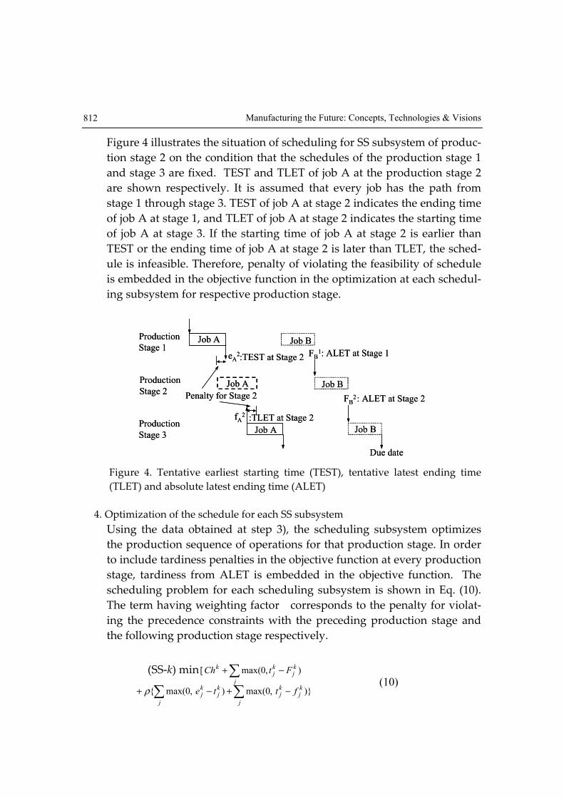
Figure 4 illustrates the situation of scheduling for SS subsystem of produc-
tion stage 2 on the condition that the schedules of the production stage 1
and stage 3 are fixed. TEST and TLET of job A at the production stage 2
are shown respectively. It is assumed that every job has the path from
stage 1 through stage 3. TEST of job A at stage 2 indicates the ending time
of job A at stage 1, and TLET of job A at stage 2 indicates the starting time
of job A at stage 3. If the starting time of job A at stage 2 is earlier than
TEST or the ending time of job A at stage 2 is later than TLET, the sched-
ule is infeasible. Therefore, penalty of violating the feasibility of schedule
is embedded in the objective function in the optimization at each schedul-
ing subsystem for respective production stage.
Figure 4. Tentative earliest starting time (TEST), tentative latest ending time
(TLET) and absolute latest ending time (ALET)
4. Optimization of the schedule for each SS subsystem
Using the data obtained at step 3), the scheduling subsystem optimizes
the production sequence of operations for that production stage. In order
to include tardiness penalties in the objective function at every production
stage, tardiness from ALET is embedded in the objective function. The
scheduling problem for each scheduling subsystem is shown in Eq. (10).
The term having weighting factor corresponds to the penalty for violat-
ing the precedence constraints with the preceding production stage and
the following production stage respectively.
(SS-k) min ∑ −+j
kj
kj
k FtCh ),0max([
∑ ∑ −+−+j j
kj
kj
kj
kj ftte )},0max(),0max({ρ
(10)
Production
Stage 1
Production
Stage 2
Production
Stage 3
Job A
Job A
eA2
Job A
fA2
Due date
FB2
FB1
Job B
Job B
Job B
:TEST at Stage 2
:TLET at Stage 2
: ALET at Stage 1
: ALET at Stage 2Penalty for Stage 2
Production
Stage 1
Production
Stage 2
Production
Stage 3
Job A
Job A
eA2
Job A
fA2
Due date
FB2
FB1
Job B
Job B
Job B
:TEST at Stage 2
:TLET at Stage 2
: ALET at Stage 1
: ALET at Stage 2Penalty for Stage 2

An Autonomous Decentralized Supply Chain Planning and Scheduling System 813
s.t. Eq. (9)
where,
- k
jt is the starting time of operation for job j at stage k .
The optimization problem (SS- k ) for each SS subsystem is solved by using
Simulated Annealing (SA) method combined with a neighbourhood search al-
gorithm (Nishi et al., 2000b). The outline of the scheduling algorithm is com-
posed of the following steps.
a) Generate an initial production sequence of operations and calculate the
starting times of operations, and calculate the objective function.
b) Select an operation randomly and insert the selected operation into a
randomly selected position, thereby change the processing order of op-
erations.
c) For a newly generated production sequence, calculate the starting times
of operations by the forward simulation and calculate the objective
function. And then decide whether the newly generated schedule is
adopted or not by using the criterion of simulated annealing method.
d) Repeat the procedure (b) to (c) for a predetermined number of times
( SN ) at the same temperature parameter ( SAT ), then the temperature pa-
rameter is reduced SASA TT η← , where η is annealing ratio. Then repeat
(b) to (d) for a predetermined number of times ( AN ).
A production schedule with a minimum objective function is regarded as the
current optimal sequence. From the results of production sequence obtained
by the simulated annealing method, the starting times of operations are calcu-
lated and the production amount of each products in each time period SS
tiP, is
calculated by using the schedule generated by the simulated annealing
method. In the proposed system, any scheduling model and any optimization
algorithm can be adopted in the scheduling subsystem. Therefore, the pro-
posed system can easily applicable to many types of scheduling problems such
as jobshop problem (Hasebe et al., 1994), flowshop problem with intermediate
storage constraints (Nishi et al., 2000c) by changing the algorithm of starting
time calculation.
Manufacturing the Future: Concepts, Technologies & Visions 814
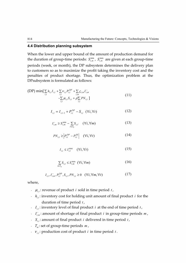
4.4 Distribution planning subsystem
When the lower and upper bound of the amount of production demand for
the duration of group-time periods: min
,miS , max
,miS are given at each group-time
periods (week, or month), the DP subsystem determines the delivery plan
to customers so as to maximize the profit taking the inventory cost and the
penalties of product shortage. Thus, the optimization problem at the
DPsubsystem is formulated as follows:
(DP) min[∑ ∑ ∑ −++ti ti mi
mimiDPtitititi IPIh
, , ,,,,,,, ςν
∑ ∑+−ti ti
tititi PNS, ,
,,, ρµ ] (11)
),(,,1,, tiSPII ti
DP
tititi ∀∀−+= − (12)
∑∈
− −≥kTt
timimi SSI'
',min,, ),( mi ∀∀ (13)
SSti
DPtiti PPPN ,,, −≥ ),( ti ∀∀ (14)
max,, titi II ≤ ),( ti ∀∀ (15)
∑∈
≤mTt
miti SS max,, ),( mi ∀∀ (16)
0,,,, ,,,,, ≥−titi
DPtimiti PNSPII ),,( tmi ∀∀∀ (17)
where,
- ti,µ : revenue of product i sold in time period t ,
- tih , : inventory cost for holding unit amount of final product i for the
duration of time period t ,
- tiI , : inventory level of final product i at the end of time period t ,
- −
miI , : amount of shortage of final product i in group-time periods m ,
- tiS , : amount of final product i delivered in time period t ,
- mT : set of group-time periods m ,
- ti,ν : production cost of product i in time period t .

An Autonomous Decentralized Supply Chain Planning and Scheduling System 815
Eq. (11) is the objective function of DP subsystem which is the sum of the
inventory holding cost for final products, production costs, penalty for
product shortage, revenue of products and penalty for violating the con-
straints with SS subsystem. Eq. (12) indicates a material balance equation
around the storage space for final product. Eq. (13) indicates the con-
straints on the minimum demand. Eq. (14) indicates the penalty value for
violating the constraints imposed by the scheduling subsystem. Eq. (15)
shows the capacity constraints of holding the final products in the storage
space. Eq. (16) denotes the constraint of maximum amount of delivery to
customer. Eq. (17) indicates the non-negative value constraints of all the
decision variables.
4.5 Overall optimization algorithm
The total subsystem derives a feasible schedule by the following steps.
Step 1. Preparation of the initial data.
Each subsystem contacts the database and obtains the data and
initializes the weighting factor of the penalty term, e.g. 0←ρ .
Step 2. Generation of an initial solution.
Each subsystem independently generates a solution without con-
sidering the other subsystems.
Step 3. Exchanging the data.
Each subsystem contacts the other sub-systems and exchanges the
amount of product data: MRP
tiP , , SS
tiP , , DP
tiP , .
Step 4. Judging whether the optimization at each subsystem is skipped or not.
To avoid cyclic generation of same solutions, each subsystem skips
Step 5 with a predetermined probability (see Hasebe et al., 1994).
Step 5. Optimization at each subsystem.
By using the data obtained at step 3, each subsystem executes the
optimization of each subproblem.
Step 6. Judging the convergence.
When the solutions of all subsystems satisfy both of the following
conditions, all of the subsystems stop the calculation, and the de-
rived solution is regarded as the final solution.
- The solution generated at Step 5 is the same as that generated at
Step 5 in the previous iteration.
Manufacturing the Future: Concepts, Technologies & Visions 816
- The value of the penalty function embedded in the objective
function is equal to zero.
Step 7. Updating the weighting factor.
If the value of penalty function is positive, the derived solution is
infeasible. Therefore, in order to reduce the degree of infeasibility,
the weighting factor of the penalty term is increased. The value of
weighting factor for penalty is updated by ρρρ Δ+← at each it-
eration. Then return to Step 3. The incremental value ρΔ is a con-
stant. If the value of ρΔ is larger, the performance index of solu-
tion derived by the proposed system becomes worse, on the other
hand, the total computation time becomes shorter. On the con-
trary, if the value of ρΔ is smaller, the total computation time is
increased while the value of performance index has been im-
proved. Our numerical studies show that when ρΔ is less than
0.5, the computation time becomes exponentially larger even
though the performance is not so improved. From these results,
we have determined 5.0=Δρ as shown in Table 8.
By taking the above algorithm, it is easy for the proposed system to intro-
duce the parallel processing system using multiple computers in which
each subsystem execute its optimization concurrently. Figure 5 is a diagram
showing the data exchange algorithm of the proposed system. Each square
in Figure 5 illustrates steps of the data exchange algorithm in the iteration
of the optimization at the subsystem and each arrow represents the flow of
data. The total number of the processors required for solving the supply
chain optimization problem is 5 processors for 3-stage production proc-
esses. The dotted arrow indicates the data of the production amount of
each product in each time period determined by the MRP subsystem and
DP subsystem. The thick arrow indicates the tentative earliest starting time
(TEST) and tentative latest starting time (TLET) which are exchanged a-
mong the SS subsystems. In each iteration step, the data of the amount of
products in each time period calculated in each subsystem are transmitted.
Then, the data of TEST and TLST are exchanged. Therefore, jobs are gener-
ated at each iteration in the proposed system. While repeating the data ex-
change among each subsystem, the number of jobs and the starting time of
operations are gradually satisfied with the constraints among each subsys-
tem.

An Autonomous Decentralized Supply Chain Planning and Scheduling System 817
Figure 5. Data exchange algorithm
5. Computational results
The proposed scheduling system is applied to a supply chain optimization
problem. The MRP subsystem and the DP subsystem is solved by a commer-
cial MILP solver (CPLEX8.0 iLOG©). The algorithm used in the scheduling
subsystem is coded by C++ language. Pentium IV (2.0AGHz) processor is used
for computation.
5.1 Example problem
A batch plant treated in the example problem consists of three production sta-
ges shown in Figure 6. In this example, it is assumed that the production
paths of all jobs are the same, meaning the each job is processed at stages 1
through 3. In this plant, four kinds of products are produced by each of two
kinds of raw materials. Product A or B is produced from material 1, and prod-
uct C and D is produced from material 2. The total planning horizon is 12
days, and it is divided into 12 time periods in the MRP subsystem and in the
DP subsystem. The shipping of raw material for each material is available only
two times in 4 days (1, 4, 7, 10). For each product, the lower bound and the
upper bound of the production demand for each 4 days are given as the ag-
SS
sub-systemWP
sub-system
MRP
sub-system
Iter
atio
n
1
2
{PitMRP} {Pit
OSP}
{PitSS}
{PitSS}
{PitSS}
{PitSS}
{PitMRP} {Pit
OSP}
SS
sub-systemWP
sub-system
MRP
sub-system
Iter
atio
n
1
2
{PitMRP} {Pit
OSP}
{PitSS}
{PitSS}
{PitSS}
{PitSS}
{PitMRP} {Pit
OSP}

Manufacturing the Future: Concepts, Technologies & Visions 818
gregated value for each product. Thus, the delivery date can be decided by the
DP subsystem. The plant is operated 24 hours/day. The available space for in-
ventory for raw material and final products are restricted. The tables 1 to 8
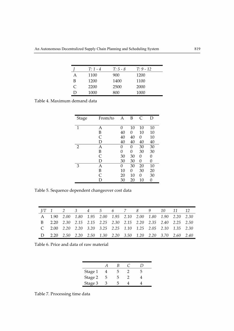
show the data and parameters used in the example problem.
Raw material 1
for A, B
A
B
C
DStorage space
for raw materialStorage space
for final products
Stage2 Stage3Stage1Raw material 2
for C, D
Raw material 1
for A, B
A
B
C
DStorage space
for raw materialStorage space
for final products
Stage2 Stage3Stage1Raw material 2
for C, D
Figure 6. 3-stage production process for the example problem
J/T 1 2 3 4 5 6 7 8 9 10 11 12
A 1.90 2.00 1.80 1.95 2.00 1.95 2.10 2.00 1.80 1.90 2.20 2.30
B 2.20 2.30 2.15 2.15 2.25 2.30 2.15 2.20 2.35 2.40 2.25 2.50
C 2.00 2.20 2.20 3.20 3.25 2.25 1.10 1.25 2.05 2.10 1.35 2.30
D 2.20 2.50 2.20 2.50 1.30 2.20 3.50 1.20 2.20 3.70 2.60 2.40
Table 1. Revenue of products at each time period
J T: 1 - 4 T: 5 - 8 T: 9 - 12
A 0.45 0.45 0.45
B 0.45 0.45 0.45
C 0.60 0.60 0.60
D 0.60 0.60 0.60
Table 2. Production costs
J T: 1 - 4 T: 5 - 8 T: 9 - 12
A 100 200 100
B 100 200 400
C 200 300 300
D 100 100 400
Table 3. Minimum demand data
An Autonomous Decentralized Supply Chain Planning and Scheduling System 819
J T: 1 - 4 T: 5 - 8 T: 9 - 12
A 1100 900 1200
B 1200 1400 1100
C 2200 2500 2000
D 1000 800 1000
Table 4. Maximum demand data
Stage
From/to A B C D
A 0 10 10 10 B 40 0 10 10 C 40 40 0 10
1
D 40 40 40 40 A 0 0 30 30 B 0 0 30 30 C 30 30 0 0
2
D 30 30 0 0 A 0 30 20 10 B 10 0 30 20 C 20 10 0 30
3
D 30 20 10 0
Table 5. Sequence dependent changeover cost data
J/T 1 2 3 4 5 6 7 8 9 10 11 12
A 1.90 2.00 1.80 1.95 2.00 1.95 2.10 2.00 1.80 1.90 2.20 2.30
B 2.20 2.30 2.15 2.15 2.25 2.30 2.15 2.20 2.35 2.40 2.25 2.50
C 2.00 2.20 2.20 3.20 3.25 2.25 1.10 1.25 2.05 2.10 1.35 2.30
D 2.20 2.50 2.20 2.50 1.30 2.20 3.50 1.20 2.20 3.70 2.60 2.40
Table 6. Price and data of raw material
A B C D
Stage 1 4 5 2 5
Stage 2 5 5 2 4
Stage 3 3 5 4 4
Table 7. Processing time data

Manufacturing the Future: Concepts, Technologies & Visions 820
Other data
Unit Volume (V1): 100, Cmax : 3000 , Imax: 300, Mmax:4000 Inventory holding cost for raw material: 0.001 Inventory holding cost for final product: 0.2 Penalty of product shortage: 4.0
Parameters for simulated annealing
Annealing times ( AN ): 400
Search times ( SN ): 200
Annealing Ratio: 0.97
Initial temperature: initial performance *0.1
Parameters for the proposed system
Skipping probability: 0.2%
Increment of weighting factor ( ρΔ ): 0.5
Table 8.Parameters used for computation
5.2 Results of coordination
Figure 7. Intermediate result after 10 times of data exchange
An Autonomous Decentralized Supply Chain Planning and Scheduling System 821
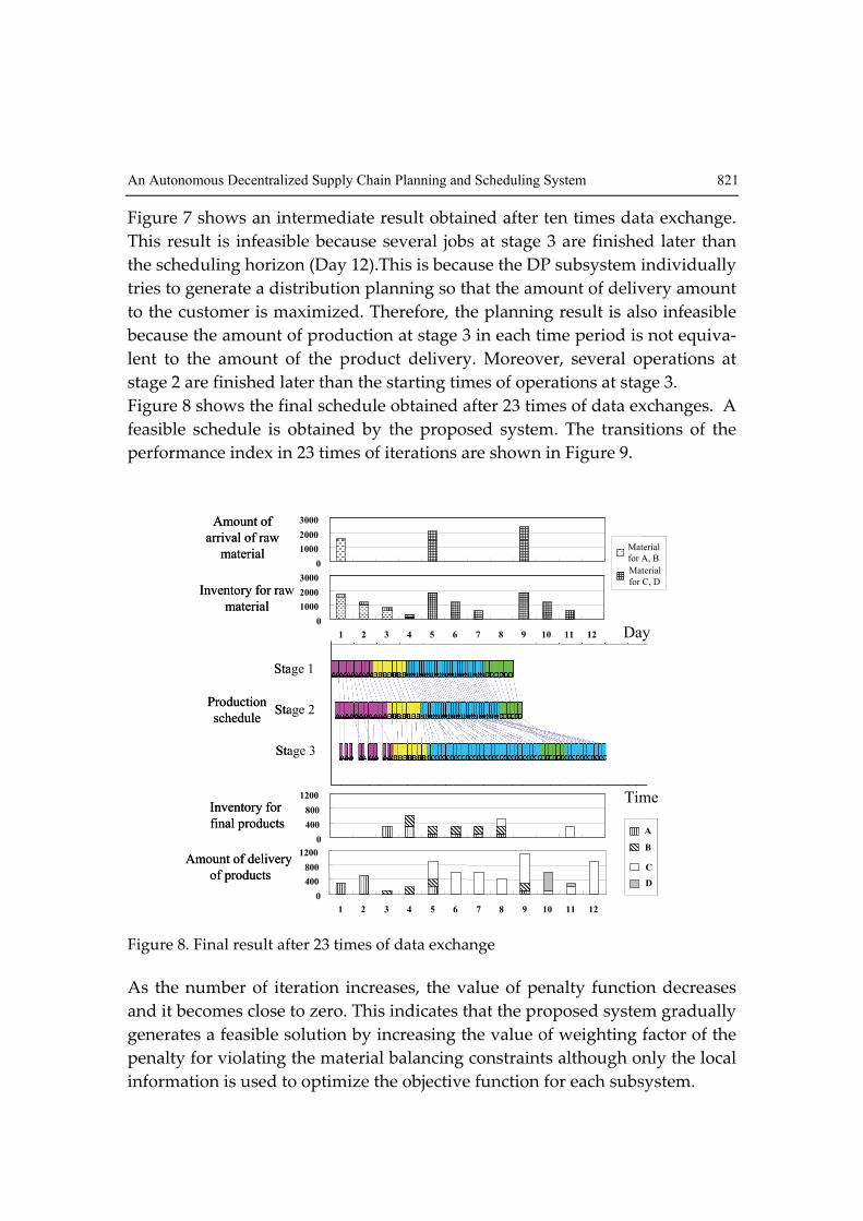
Figure 7 shows an intermediate result obtained after ten times data exchange.
This result is infeasible because several jobs at stage 3 are finished later than
the scheduling horizon (Day 12).This is because the DP subsystem individually
tries to generate a distribution planning so that the amount of delivery amount
to the customer is maximized. Therefore, the planning result is also infeasible
because the amount of production at stage 3 in each time period is not equiva-
lent to the amount of the product delivery. Moreover, several operations at
stage 2 are finished later than the starting times of operations at stage 3.
Figure 8 shows the final schedule obtained after 23 times of data exchanges. A
feasible schedule is obtained by the proposed system. The transitions of the
performance index in 23 times of iterations are shown in Figure 9.
0
1000
2000
3000
1 2 3 4 5 6 7 8 9 10 11 12
0
1000
2000
3000
1 2 3 4 5 6 7 8 9 10 11 12
Stage 1
Stage 2
Stage 3
Inventory for
final products
Amount of delivery
of products
Inventory for raw
material
Amount of
arrival of raw
material
Day
Material
for A, B
Material
for C, D
Production
schedule
0
400
800
1200
1 2 3 4 5 6 7 8 9 10 11 12
0
400
800
1200
1 2 3 4 5 6 7 8 9 10 11 12
D
C
B
A
Time
0
1000
2000
3000
1 2 3 4 5 6 7 8 9 10 11 12
0
1000
2000
3000
1 2 3 4 5 6 7 8 9 10 11 12
Stage 1
Stage 2
Stage 3
Inventory for
final products
Amount of delivery
of products
Inventory for raw
material
Amount of
arrival of raw
material
Day
Material
for A, B
Material
for C, D
Production
schedule
0
400
800
1200
1 2 3 4 5 6 7 8 9 10 11 12
0
400
800
1200
1 2 3 4 5 6 7 8 9 10 11 12
0
400
800
1200
1 2 3 4 5 6 7 8 9 10 11 12
0
400
800
1200
1 2 3 4 5 6 7 8 9 10 11 12
D
C
B
A
D
C
B
A
Time
Figure 8. Final result after 23 times of data exchange
As the number of iteration increases, the value of penalty function decreases
and it becomes close to zero. This indicates that the proposed system gradually
generates a feasible solution by increasing the value of weighting factor of the
penalty for violating the material balancing constraints although only the local
information is used to optimize the objective function for each subsystem.

Manufacturing the Future: Concepts, Technologies & Visions 822
0
5000
10000
15000
20000
25000
30000
35000
40000
1 11 21 31 41 51
Iteration [-]
Per
form
ance
in
dex
[-]
Material Cost
Changeover cost
Revenue of product
Production cost
Penalty function
Figure 9. The transitions of the performance index
5.3 Comparison of the proposed system and the conventional system
In order to evaluate the performance of the proposed system, a hierarchical
planning and scheduling system considering the entire plant is also developed.
The planning problem (HP) is formulated as MILP problem by using the mid-
term-planning model proposed by McDonald & Karimi (1997).
(HP) Zmin ∑ ∑ ∑++=tr tr ti
tititrtrtrtr PCqMpZ, , ,
,,,,,, ν
∑ ∑ ∑−++ −
ti mi tititimimititi SIIh
, , ,,,,,,, µς (18)
),(,,1,, trPMCC
rUi
titrtrtr ∀∀−+= ∑∈
− (19)
),(max,, tiCC titi ∀∀≤ (20)
∑ ∀≤t
rtr rmY )(, (21)
),(/, ltHVPs t
i
ltili ∀∀≤⋅∑ (22)

An Autonomous Decentralized Supply Chain Planning and Scheduling System 823
),(,,1,, tiSPII titititi ∀∀−+= − (23)
),(max,, tiII titi ∀∀≤ (24)
),('
',min,, miSSI
mTt
timimi ∀∀−≥ ∑∈
− (25)
),(0,,,,, ,,,,,, tiSIICMP titititititi ∀∀≥− (26)
),(}1,0{, tiY ti ∀∀∈ (27)
where,
- tH : amount of time available in the time period t ,
- mT : set of group-time period m ,
- tV : batch size of the machine at the production stage l .
For the hierarchical approach, the solution of the HP problem is transferred to
the scheduling subsystem as the production request. The jobs are created by
using the production amount: tiP , calculated in the planning system. The sche-
duling system obtains the amount of inventory for raw material, due dates for
each job. And then the scheduling system is executed. For the scheduling
system used in the hierarchical approach, a schedule considering the entire
production stages is successively generated improving an initial schedule. The
simulated annealing method is adopted so that the solution is not trapped in a
local optimal.
Ten times of calculations are made with different seed numbers for generating
random numbers in the simulated annealing method to compare the perform-
ance of the proposed system. The results of the performance index for the pro-
posed system (DSCM1) and the hierarchical planning and scheduling system
(CONV) are shown in Table 10. The average computation time for deriving a
feasible schedule of the proposed algorithm is 198 seconds. The performance
of the DSCM1 is lower than that of the hierarchical system (CONV). This is be-
cause some of the solutions of the schedule generated by each subsystem have
been entirely different from that derived by other subsystem, which makes
convergence of the proposed algorithm difficult. Thereby, the final solution of
the proposed system has been trapped into a bad local optimum. In order to
improve the efficiency of the proposed method, the capacity constraints for

Manufacturing the Future: Concepts, Technologies & Visions 824
each month are embedded into the DP subproblem. By adding the capacity
constraints to DP subproblem, the number of generating meaningless solutions
violating the constraints with the SS subsystem has been reduced. The results
of computation for the improved method (DSCM2) are shown in Table 10. The
profit of DSCM2 is successfully improved compared with that of DSCM1
without sacrificing the computational expenses. For DSCM2, the changeover
cost is lower than that of CONV, though the profit for final products is higher
than CONV. This is because both the changeover costs and the profit of the
product greatly depend on the production schedule, and it is very difficult for
CONV to determine the precise production schedule at the production plan-
ning level. It is demonstrated that the total profit of proposed system (DSCM2)
is higher than that of the conventional system (CONV). The proposed system
can generate a better solution than the conventional system even though only
local information is used to generate the solution of each subsystem.
6. Conclusion and future work
An autonomous decentralized supply chain optimization system for multi-
stage production processes has been proposed. The novel aspect of this paper
is that we provide a novel distributed optimization system for a supply chain
planning problem for multi-stage production processes comprising a material
requirement planning (MRP) subsystem, scheduling subsystems for each pro-
duction stage, and a distribution planning (DP) subsystem.
Methods DSCM1 DSCM2 CONV
Number of data exchange 18 21 1
Profit [-] 7,533 9,538 9,418
Number of jobs [-] 66 66 62
Total revenue [-] 14,353 15,759 15,460
Costs of raw material [-] 1,540 1,688 1,677
Inventory cost for raw materials [-] 18 21 26
Inventory holding cost for final products [-] 504 720 360
Production cost [-] 2,970 3,006 2,790
Penalty of product shortage [-] 1320 360 400
Sequence dependent changeover cost [-] 468 426 1,030
Table 10. Comparison of the autonomous decentralized supply chain planning
system (DSCM) and the conventional system (CONV)

An Autonomous Decentralized Supply Chain Planning and Scheduling System 825
Each subsystem includes an optimization function and repeats the generation
of solutions for each subproblem and data exchange among the subsystems.
The total system derives a feasible solution by gradually increasing the weight-
ing factor for violating the infeasibility of the solution through repeated opti-
mization at each subsystem and data exchanges among the subsystems. The
data exchanged among the subsystems are tentative production amount of
each product at each time period that is desirable for each subsystem. By
adopting such a structure, it is easy to modify the subsystem when a new con-
straint is added or when performance evaluation criteria changes. Thus, the
system can flexibly accommodate various unforeseen changes. he proposed
system is successfully applied to a multi-stage supply chain optimization prob-
lem. The results demonstrate that feasible solutions could be obtained by the
numerical examples. The performances of the proposed system are compared
with those of the schedule derived by the conventional system. It has been
shown that the proposed system can generate a better solution than the con-
ventional system without sacrificing flexibility and computational resources.
Future work should be investigated on how to optimize the entire supply
chain under several uncertainties.
7. Nomenclature
- trC , : amount of inventory of raw material r at the end of time period t,
- max
,trC : maximum amount of inventory for raw material r at the end of time
period t,
- kCh : sequence dependent changeover cost at stage k,
- k
je : tentative earliest starting time of job i at stage k,
- k
jf : tentative latest ending time of job i at stage k,
- k
jF : absolute latest ending time of job j at stage k ,
- tih , : inventory cost for holding unit amount of final product i for the du-
ration of time period t,
- tiI , : inventory level of final product i at the end of time period t,
- max
,tiI : maximum amount of inventory for final product i at the end of time
period t,
- −
miI , : amount of shortage of inventory for final product i in group-time
periods m,
- K : sufficiently large positive number,

Manufacturing the Future: Concepts, Technologies & Visions 826
- rm : maximum number of the arrival of raw material r ,
- trM , : amount of raw material r arrived from supplier at the start of time
period t,
- AN : annealing time for simulated annealing,
- SN : search times at the same temperature for simulated annealing,
- trp , : price of the unit amount of raw material r from supplier to the plant
at the start of time period t,
- MRP
tiP, tentative amount of production of product i in time period t, which
is derived at MRP subsystem,
- DP
tiP , : tentative amount of production of product i in time period t, which
is derived at DP subsystem,
- SS
tiP , : tentative amount of production of product i in time period t, which
is derived at DP subsystem,
- tiPN , : difference of production amount of product i in time period t,
- trq , : inventory holding cost of unit amount of raw material r for the
duration of time period t,
- k
is : processing time of operation for job j at stage k ,
- tiS , : amount of final product i delivered in time period t,
- k
jt : starting time of operation for job j at stage k ,
- mT : set of time in group-time periods m,
- availableT periods of time when the material arrival is available,
- SAT : annealing temperature for simulated annealing method,
- TEST tentative earliest starting time,
- TLET tentative latest ending time, rU : set of products produced
- from material r ,
- lV : batch size of the machine at the production stage l,
- trY , : binary variable indicating whether material r is arrived at the start
of time period t or not.
Greek Letters
- η : annealing ratio ( temperature reduction factor),
- ti,µ : revenue of of product i sold in time period t,
- ti,ν : production cost of product i in time period t,
- ρ : penalty parameter,
- mi,ς : penalty for unit amount of shortage of product in group-time
- periods m ,

An Autonomous Decentralized Supply Chain Planning and Scheduling System 827
8. References
Androulakis, I. and Reklaitis, G. (1999), Approaches to Asynchronous Decen-
tralized Decision Making, Computers and Chemical Engineering, Vol. 23, pp.
341-355.
Birewar, D. and Grossmann, I. (1990) Production Planning and Scheduling in
Multiproduct Batch Plants, Ind. Eng. Chem. Res., Vol. 29, 570-580.
Bitran, R., Hax, A. (1977) On the Design of Hierarchical Production Planning
Systems, Decision Sciences, Vol. 8, pp. 29-55.
Bok, J.K., Grossmann, I.E., Park, S. (2000) Supply Chain Optimization in Con-
tinuous Flexible Process, Ind. Eng. Chem. Res., Vol. 39, pp. 1279-1290.
Burke, P., Prosser, P., (1990) Distributed Asynchronous Scheduling, Applica-
tions of Artificial Intelligence in Engineering V, Vol. 2, pp. 503-522.
Gou, L., Luh, P.B. Luh, Kyoya, Y. (1998) Holonic manufacturing scheduling:
architecture, cooperation mechanism, and implementation, Computers in
Industry, Vol. 37, pp. 213-231.
Gupta, A., Maranas, C.D. (1999) Hierarchical Lagrangean Relaxation Procedure
for Solving Midterm Planning Problems, Ind. Eng. Chem. Res., Vol. 38,
pp. 1937-1947
Hasebe, S., Kitajima, T., Shiren, T., Murakami, Y. (1994) Autonomous Decen-
tralized Scheduling System for Single Production Line Processes, Pre-
sented at AIChE Annual Meeting, Paper 235c, USA.
Hoitomt, D.J., Luh, P.B., Pattipati, R. (1993) A Practical Approach to Job-Shop
Scheduling Problems, IEEE Trans. Robot. Automat., Vol. 9, pp. 1-13.
Jeremy, F. S. (2001) Modeling the Supply Chain, Thomson Learning.
Fischer, K. (1999) Agent-based design of holonic manufacturing systems, Ro-
botics and Autonomous Systems, Vol. 27, pp. 3-13.
Maturana, F.P., Norrie, D.H., (1997) Distributed decision-making using the
contract net within a mediator architecture, Decision Support Systems, Vol.
20, pp. 53-64.
McDonald, C. and Karimi, I. (1997), Planning and Scheduling of Parallel Semi-
continuous Processes. 1. Production Planning, Ind. Eng. Chem. Res., Vol.
36, pp. 2691-2700.
Mckay, A., Pennington, D., Barnes, C. (2001) A Web-based tool and a heuristic
method for cooperation of manufacturing supply chain decisions, Vol. 12,
pp. 433-453.

Manufacturing the Future: Concepts, Technologies & Visions 828
Nishi, T., Inoue, T., Yutaka, H., Taniguchi, S. (2000a) Development of a Decen-
tralized Supply Chain Optimization System, Proceedings of the Interna-
tional Symposium on PSE Asia, 141-146.
Nishi, T., Konishi, M., Hattori, Y., Hasebe, S. (2003) A Decentralized Supply
Chain Optimization Method for Single Stage Production Systems, Trans-
actions of the Institute of Systems, Control and Information Engineers, 16-12,
628-636 (in Japanese)
Nishi, T., Sakata, A., Hasebe, S., Hashimoto, I. (2000b), Autonomous Decentral-
ized Scheduling System for Just-in-Time Production, Computers and
Chemical Engineering, Vol. 24, pp. 345-351.
Nishi, T., Sakata, A., Hasebe, S., Hashimoto, I. (2000c), Autonomous Decentral-
ized Scheduling System for flowshop problems with storage cost and
due-date penalties, Kagaku Kogaku Ronbunshu, Vol. 26, pp. 661-668 (in
Japanese).
Ohkuma, K., Ueda, K., (1996) Solving Production Scheduling Problems with
a Simple Model of Biological-Oriented Manufacturing Systems, Nihon
Kikaigakkai Ronbunshu C, Vol. 62, pp. 429-435, 1996 (in Japanese).
Rupp, T.M., Ristic, M. (2000) Fine Planning for Supply Chains in Semiconduc-
tor Manufacture, Journal of Material Processing Technology, Vol. 107, pp.
390-397.
Shaw, M.J., (1987) A distributed scheduling method for computer integrated
manufacturing: the use of local area network in cellular systems, Int. J.
Prod. Res., Vol. 25, No. 9, pp. 1285-1303.
Simon, C., Pietro, R., Mihalis G. (2000) Supply chain management: an analytical
framework for critical literature review, European Journal of Purchasing&
Supply Management, Vol. 6, pp. 67-83.
Smith, R.G., (1980) The Contract Net Protocol: High-Level Communication
Control in a Distributed Problem Solver, IEEE Transactions on Computers,
Vol. 29, No.12, pp. 1104-1113.
Tan, M., (2001) Hierarchical Operations and Supply Chain Planning, Springer.
Tharumarajah, A., Bemelman, R., (1997) Approaches and issues in scheduling a
distributed shop-floor environment, Computers in Industry, Vol. 34, pp.
95-109.
Vidal, C.J. and Goetschalckx, M. (1997) Strategic production-distribution mod-
els: A critical review with emphasis on global supply chain models, Euro-
pean Journal of Operational Research, Vol. 98, pp. 1-18.
Wei, T., (2000) Integration of Process Planning and Scheduling - a Review,
Journal of Intelligent Manufacturing, Vol. 11, pp. 51-63.
Manufacturing the FutureEdited by Vedran Kordic, Aleksandar Lazinica and Munir Merdan
ISBN 3-86611-198-3Hard cover, 908 pagesPublisher Pro Literatur Verlag, Germany / ARS, Austria Published online 01, July, 2006Published in print edition July, 2006
InTech EuropeUniversity Campus STeP Ri Slavka Krautzeka 83/A 51000 Rijeka, Croatia Phone: +385 (51) 770 447 Fax: +385 (51) 686 166www.intechopen.com
InTech ChinaUnit 405, Office Block, Hotel Equatorial Shanghai No.65, Yan An Road (West), Shanghai, 200040, China
Phone: +86-21-62489820 Fax: +86-21-62489821
The primary goal of this book is to cover the state-of-the-art development and future directions in modernmanufacturing systems. This interdisciplinary and comprehensive volume, consisting of 30 chapters, covers asurvey of trends in distributed manufacturing, modern manufacturing equipment, product design process,rapid prototyping, quality assurance, from technological and organisational point of view and aspects of supplychain management.
How to referenceIn order to correctly reference this scholarly work, feel free to copy and paste the following:
Tatsushi Nishi (2006). An Autonomous Decentralized Supply Chain Planning and Scheduling System,Manufacturing the Future, Vedran Kordic, Aleksandar Lazinica and Munir Merdan (Ed.), ISBN: 3-86611-198-3,InTech, Available from:http://www.intechopen.com/books/manufacturing_the_future/an_autonomous_decentralized_supply_chain_planning_and_scheduling_system