An Attempt of Image Segmentation Based onBayesian Decision Rule and Maximum Likelihood

MethodJunyi Feng

School of Information Science and TechnologyShanghaitech University

Pudong, ShanghaiEmail: fengjy@shanghaitech.edu.cn

ID: 34590148

Abstract—In this article, an algorithm to solve image fore-ground and background matting is proposed. Different frompopular algorithms, a method that uses Bayesian Decision Rule,Maximum-likelihood estimation will be described. The algorithm-s will be discussed. Some tests will be shown and the performanceof this method will be discussed. What’s more, note that this workis the final project of EE251–Signal Estimation and Detectiontheory and this is the summary of the work.

Index Terms—Bayesian Decision Rule, Image Segmentation,Matting

I. INTRODUCTION

Nowadays, image segmentation, image matting technologieshas been well developed. This kind of technologies has beenwidely used in medical image processing, geographic imageprocessing, object proposal, detection and other related areas.There has been lot of excellent algorithms proposed by en-gineers and scientists in Computer Vision area, like K-meansClustering, Texture filters, Graph Cut, and CNN algorithms.While in this class, we’ve learnt a lot of methods that basedon probability(parameter-noise-observation) model, this is themotivation that I tried to model the images as signals, createthe observations and estimate/detect the parameters.

The algorithm aims to deal with a 2-segmentation problem.Given an input image, the algorithm should judge whethereach pixel belongs to foreground or background. For eachpixel, we choose its right-below(including itself) 8*8 sub-image as our observation. The DCT(discrete cosine transform)is performed, and the distribution of these 64 coefficients willbe trained, and the Bayesian detection(classification) methodswill be used to finish the segmentation.

II. INTRODUCTION TO ALGORITHM

This problem is indeed a 2-classification problem. Eachpixel in the intensity image I(i, j) has its type Y (0 or 1),which represents whether this pixel belongs to the backgroundor foreground, is what we want to estimate. We use the DCT

coefficients of its nearby 8*8 sub-figure to be the observationXij. The following part will describe the algorithm and showthe principle in detail.

A. Variable Construction

First, we define the type random variable Y as

Y =

{0, pixel ∈ background,1, pixel ∈ object (foreground)

Next, the observation should be modeled. To include thelocal information, the neighbor-region of each pixel should beconsidered, thus, the right-bottom 8*8 region is used. What’smore, we perform DTC (Discrete Cosine Transform) so thatthe frequency coefficients, which are more general to be viewas features, are calculated and used as our observation for eachpixel. The principle is shown in the following figure.

Fig. 1. Observation Construction

After the procedure, we will obtain a vector of size 64as the observation for each pixel. It’s reasonable that undereach type(background and object), the joint distribution of theobservation vectors are not the same, which are what we cantrain from the training image and the corresponding groundtruth mask images.

B. Generation of Training Data

A series of training images and the corresponding mask(ofobject) images will be used. For each training image, wescan all of its pixels and calculate the feature vector usingthe method in A. Then, use 2 matrices(Back features, Ob-j features) to store feature vectors according to the mask ofthe current pixel. The procedure is shown in Fig. 2.

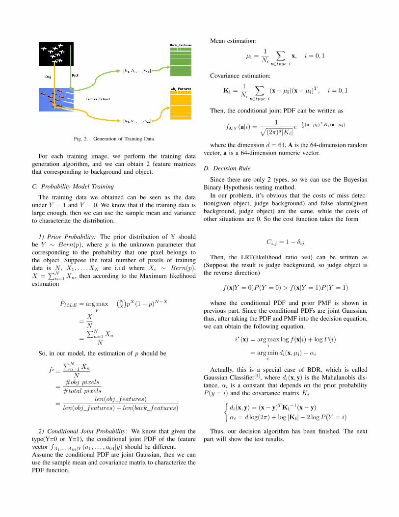
Fig. 2. Generation of Training Data

For each training image, we perform the training datageneration algorithm, and we can obtain 2 feature matricesthat corresponding to background and object.

C. Probability Model Training

The training data we obtained can be seen as the dataunder Y = 1 and Y = 0. We know that if the training data islarge enough, then we can use the sample mean and varianceto characterize the distribution.

1) Prior Probability: The prior distribution of Y shouldbe Y ∼ Bern(p), where p is the unknown parameter thatcorresponding to the probability that one pixel belongs tothe object. Suppose the total number of pixels of trainingdata is N , X1, . . . , XN are i.i.d where Xi ∼ Bern(p),X =

∑Nn=1Xn, then according to the Maximum likelihood

estimation

P̂MLE = argmaxp

(NX

)pX(1− p)N−X

=X

N

=

∑Nn=1Xn

N

So, in our model, the estimation of p should be

P̂ =

∑Nn=1Xn

N

=#obj pixels

#total pixels

=len(obj features)

len(obj features) + len(back features)

2) Conditional Joint Probability: We know that given thetype(Y=0 or Y=1), the conditional joint PDF of the featurevector fA1,...,A64|Y (a1, . . . , a64|y) should be different.Assume the conditional PDF are joint Gaussian, then we canuse the sample mean and covariance matrix to characterize thePDF function.

Mean estimation:

µi =1

Ni

∑x∈tpye i

x, i = 0, 1

Covariance estimation:

Ki =1

Ni

∑x∈tpye i

(x− µi)(x− µi)T , i = 0, 1

Then, the conditional joint PDF can be written as

fA|Y (a|i) =1√

(2π)d|Ki|e−

12 (a−µi)

TKi(a−µi)

where the dimension d = 64, A is the 64-dimension randomvector, a is a 64-dimension numeric vector.

D. Decision Rule

Since there are only 2 types, so we can use the BayesianBinary Hypothesis testing method.

In our problem, it’s obvious that the costs of miss detec-tion(given object, judge background) and false alarm(givenbackground, judge object) are the same, while the costs ofother situations are 0. So the cost function takes the form

Ci,j = 1− δij

Then, the LRT(likelihood ratio test) can be written as(Suppose the result is judge background, so judge object isthe reverse direction)

f(x|Y = 0)P (Y = 0) > f(x|Y = 1)P (Y = 1)

where the conditional PDF and prior PMF is shown inprevious part. Since the conditional PDFs are joint Gaussian,thus, after taking the PDF and PMF into the decision equation,we can obtain the following equation.

i∗(x) = argmaxi

log f(x|i) + logP (i)

= argmini

di(x, µi) + αi

Actually, this is a special case of BDR, which is calledGaussian Classifier[1], where di(x, y) is the Mahalanobis dis-tance, αi is a constant that depends on the prior probabilityP (y = i) and the covariance matrix Ki{

di(x, y) = (x− y)TKi−1(x− y)

αi = d log(2π) + log |Ki| − 2 logP (Y = i)

Thus, our decision algorithm has been finished. The nextpart will show the test results.

III. TEST AND RESULTS

The data set used is CMU Cornell iCoseg dataset[2],here an example of test will be shown. The images used inthis test are Airshow− Planes. Two of the images are usedfor training and one other image is used for testing.

The training images are shown in Fig. 3.

(a) Training image 1 (b) Training mask 1

(c) Training image 1 (d) Training mask 2

Fig. 3. Training images

A. Distribution estimation

After the training procedure, we obtain the conditional jointPDFs, since it’s 64-dimension, which is hard to plot, so herewill list the marginal distribution of each coefficients in thevector. Note that the the curves with red color corresponds tothe PDF of object, while blue color corresponds to PDF ofbackground.

Fig. 4. Conditional PDF 1-16

Fig. 5. Conditional PDF 17-32

Fig. 6. Conditional PDF 33-48

Fig. 7. Conditional PDF 49-64

B. Segmentation

After all of the previous work, the segmentation can beachieved, the test image is another plane figure, which isshown in Fig. 8.

Fig. 8. Test Image

The results of the algorithm compared with the ground truthis shown in Fig. 9.

(a) Algorithm output (b) Ground Truth

Fig. 9. Segmentation Result

The accuracy parameters are

P (False Alarm) = 0.0549

P (Miss Dectection) = 0.1003

P (Total Error) = 0.05744307

Here lists the result of another segmentation.

(a) Input image (b) Output Segmentation

Fig. 10. Segmentation Result

IV. CONCLUSION

According to the analysis of the performance of this BDRalgorithm, the method works well in many common cases.Especially in some cases where the object has a fixed kindof texture, and the background is not that complex. While forsome other cases where the frequency features are not thatdifferent between object and background, the algorithm mayperform not that well.

V. DISCUSSION

Here lists some limitations of the current algorithm, andsome of future works are proposed.

A. Scale-Variance

As the design of our feature descriptor, it contains thefrequency information of the local 8*8 region. This is notenough because in real cases, the scale-variant fact exists. Inthe test of Panda, the algorithm works really poor becausethere are not enough frequency-domain features in 8*8 region-s. To solve this problem, some of other feature descriptors likeSIFT[3], SURF[4] may help because of they are scale-invariant,while these kind of descriptors are more time-consuming tobe generated.

B. Uncertainty of Background

In our training step, the background could be limited, thismeans our training of background features may not work forthe situations where the background is completely differentfrom the training images. While it may work very well if thecamera is fixed in the scene, like in the monitoring system.

C. Wrong Prior

It’s possible that the real PMF is totally different fromthe prior that we calculate using the training data. The realphoto can differ a lot in terms of resolution. A method tofix this problem is to first use the prior, each time after thesegmentation, recalculate the a-posterior distribution and usethe new PMF to regenerate the segmentation, recursively runthe algorithm until the PMF converges.

D. Bad coefficients

From the marginal PDF figures we know not all thecoefficients are proper for this decision problem, for somecoefficients, its marginal PDF is almost independent of itstype. Therefore, we can first calculate the KL-Distance orTotal-Variance-Distance to measure the distance betweenthe conditional probabilities, choose the largest ones as thefeatures that will finally used.

ACKNOWLEDGMENT

The authors would like to thank to this class, it taught mea lot of method that can give me inspects when consideringmy task, even if the problem can’t be directly constructed bythe parameter-observation model. The power of probability,Bayesian model also impressed me a lot.

Although the work and method used in this project is not thesame as the latest research in computer vision, still, I learntto model the problem and see the real power of the theoryand calculation written in my homework. I really appreciateit to have the chance to design a model and see the expectedresults.

REFERENCES

[1] The Gaussian Classifier, http://www.svcl.ucsd.edu/courses/ece271A-F08/handouts/GC2.pdf

[2] D. Batra, A. Kowdle, D. Parikh, L. Jiebo, and C. Tsuhan. iCoseg:Interactive co-segmentation with intelligent scribble guidance. In CVPR,pages 3169 C3176, 2010.

[3] Lowe, David G. (1999). Object recognition from local scale-invariantfeatures. Proc. (ICCV’99) (Corfu, Greece): 1150-1157.

[4] Bay, Herbert; Tuytelaars, Tinne and van Gool, Luc (2006). SURF:Speeded up robust features. Proc. (ECCV’06) Springer Lecture Notesin Computer Science 3951: 404-417.