an assessment of plant community - ohiolink
TRANSCRIPT

AN ASSESSMENT OF PLANT COMMUNITY COMPOSITION AND STRUCTURE
OF FORESTED MITIGATION WETLANDS AND RELATIVELY UNDISTURBED
REFERENCE FORESTED WETLANDS IN OHIO
A Thesis
Presented in Partial Fulfillment of the Requirements for the Degree Master of Science in
the Graduate School of The Ohio State University
By
John Edward Reinier, B.S.
Graduate Program in Environment and Natural Resources
*****
The Ohio State University
2011
Master's Examination Committee:
Dr. David M. Hix, Advisor
Dr. Dawn R. Ferris
Dr. P. Charles Goebel

Copyrighted by
John Edward Reinier Jr.
2011

ii
ABSTRACT
The ecological functions provided by mature forested wetlands are continually
being lost through permitted impacts associated with residential, commercial and
agricultural development. In response, regulatory agencies require that forested wetlands
be restored, established, enhanced or preserved (i.e., wetland mitigation) to replace those
ecological functions. Assessments of wetland mitigation projects often focus on plant
community characteristics as indicators of ecological integrity. Using the Vegetation
Index of Biotic Integrity (VIBI) sampling protocol, we collected herbaceous and woody
plant community data as well as physical habitat attribute data at four forested mitigation
areas and four relatively undisturbed reference forested wetlands within the Erie/Ontario
Drift and Lake Plains and Eastern Corn Belt Plains ecoregions of Ohio. The objectives of
the study were to compare the plant community composition and structure of these areas
and to identify factors that may be influencing their development. Our analyses revealed
both compositional and structural differences between mitigation and reference areas and
indicated that certain physical habitat features (e.g., hummocks, macrotopographic
depressions and coarse woody debris) may influence plant community development. Past
land use, disturbance history and landscape setting also likely played an important role in
shaping the plant communities of the sampled areas. Mitigation areas supported fewer

iii
ecologically-conservative species than reference areas and lacked a subcanopy of native,
shade-tolerant wetland tree and shrub species. VIBI results indicated that reference areas
were characterized by the presence of seedless vascular plants, a high Floristic Quality
Assessment Index score, the importance of native, shade-tolerant species as well as high
percent cover of sensitive species, hydrophytes and bryophytes. Mitigation areas were
characterized by ecologically tolerant species, the importance of canopy tree species, and
many trees in small diameter classes. These results suggest that forested mitigation
wetlands may support plant communities dominated by species with a wide range of
ecological tolerance and may lack the structure that characterizes mature forested
wetlands. Assuming mitigation areas are on a desirable trajectory, several decades may
pass before areas currently used for forested wetland mitigation begin to resemble
relatively undisturbed areas in terms of plant community composition and structure. As
more and more forested wetlands are negatively impacted by residential, commercial and
agricultural development, there will likely be a continual decline in the functions
provided by mature forested wetlands throughout Ohio.

iv
ACKNOWLEDGMENTS
I owe a great deal of thanks to my family, particularly my wife, Abby, for their
support and patience throughout my academic career. I also want to thank my advisor,
Dr. David Hix for his helpful advice and encouragement over the last two and a half
years. My other two committee members, Dr. Charles Goebel and Dr. Dawn Ferris also
provided helpful comments that improved this research. While working at Ohio EPA, I
learned a great deal about wetland ecology from Mick Micacchion and Brian Gara. They
have both been instrumental in my academic and professional development. I greatly
appreciate all the assistance provided by the faculty and staff of the School of
Environment and Natural Resources. Finally, this research would not have been possible
without the SEEDS grant awarded to me by the Ohio Agricultural Research and
Development Center.
v
VITA
2008................................................................B.S. Conservation, Kent State University
2008 to 2010 .................................................Graduate Teaching Associate, School of
Environment and Natural Resources, The
Ohio State University
2010 to present ..............................................Biologist, U.S. Army Corps of Engineers,
Buffalo District - Orwell, Ohio Field Office
Fields of Study
Major Field: Environment and Natural Resources
Area of Specialization: Forest Science

vi
TABLE OF CONTENTS
Abstract ............................................................................................................................... ii Acknowledgments.............................................................................................................. iv
Vita ...................................................................................................................................... v
List of Tables .................................................................................................................... iix
List of Figures .................................................................................................................... xi Chapter 1: Introduction ....................................................................................................... 1
Chapter 2: Herbaceous Plant Community Compostion of Forested Mitigation Wetlands and Relatively Undisturbed Reference Forested Wetlands ............................................... 7
Introduction ..................................................................................................................... 8
Study Areas ................................................................................................................... 11
Physiography and Soils ............................................................................................. 12
Methods ......................................................................................................................... 13
Vegetation Data ......................................................................................................... 13
Soil Data .................................................................................................................... 14
Physical Habitat Attributes ........................................................................................ 15
Plant Species Relative Cover Values ......................................................................... 16
Statistical Analyses .................................................................................................... 16
Results ........................................................................................................................... 18
Cluster Analysis ......................................................................................................... 19
Multi Response Permutation Procedure .................................................................... 19
Nonmetric Multidimensional Scaling ........................................................................ 20
Soil Characteristics .................................................................................................... 21
Physical Habitat Attributes ........................................................................................ 21
Discussion ..................................................................................................................... 22

vii
Physical Habitat Attributes ........................................................................................ 22
Past Land Use and Disturbance History .................................................................... 24 Physiographic Factors and Landscape Position ......................................................... 24
Soil Characteristics .................................................................................................... 30
Conclusions ................................................................................................................... 30
Chapter 3: Woody Plant Community Composition and Structure of Forested Mitigation Wetlands and Relatively Undisturbed Reference Forested Wetlands .............................. 50
Introduction ................................................................................................................... 52
Study Areas ................................................................................................................... 54
Physiography and Soils ............................................................................................. 55
Methods ......................................................................................................................... 56
Vegetation Data ......................................................................................................... 56
Soil data ..................................................................................................................... 57
Physical Habitat Attributes ........................................................................................ 58
Vegetation Data Reduction and Metric Calculations ................................................ 58
Statistical Analyses .................................................................................................... 59
Results ........................................................................................................................... 62
Cluster Analysis ......................................................................................................... 63
Multi Response Permutation Procedure .................................................................... 63
Nonmetric Multidimensional Scaling ........................................................................ 63
Soil Characteristics .................................................................................................... 64
Physical Habitat Attributes ........................................................................................ 65
Discussion ..................................................................................................................... 65
Canopy Composition ................................................................................................. 65
Canopy Structure ....................................................................................................... 68
Subcanopy Composition ............................................................................................ 69
Subcanopy Structure .................................................................................................. 71
Standing Dead Trees .................................................................................................. 75
Soil Characteristics .................................................................................................... 76
Conclusions ................................................................................................................... 76
Chapter 4: Using the Vegetation Index of Biotic Integrity to Compare Forested Mitigation Wetlands and Relatively Undisturbed Reference Forested Wetlands ............ 97
Introduction ................................................................................................................... 98
viii
Study Area and Methods ............................................................................................. 100 Vegetation Data Reduction and Metric Calculations .............................................. 101
Statistical Analyses .................................................................................................. 101
Results ......................................................................................................................... 102
VIBI Metrics ............................................................................................................ 102
Nonmetric Multidimensional Scaling ...................................................................... 102
Discussion ................................................................................................................... 103
VIBI Scores ............................................................................................................. 103
Wetland Tiered Aquatic Life Use Designations ...................................................... 106
Conclusions ................................................................................................................. 107 Chapter 5: Applications and Limitations ........................................................................ 120
Bibliography ................................................................................................................... 123
Appendix A: Study Area Descriptions ........................................................................... 123

ix
LIST OF TABLES
Table Page
2.1 Summary information describing the four mitigation plots and the four relatively undisturbed reference plots………………………………………………………38
2.2 Mean (103) (± 1 standard error) relative cover values for herbaceous species in
mitigation and reference forested wetland plots. Nomenclature based on Andreas et al. (2004)……………………………………………………………………....39
2.3 Mean values of (± 1 standard error) soil characteristics from mitigation and
reference forested wetlands. An asterisk indicates a significant difference in the mean values between mitigation and reference sites (Mann-Whitney test; p < 0.05)………………………………………………………………...……………42
2.4 Mean values (± 1 standard error) of physical attributes from mitigation and
reference forested wetland plots. An asterisk indicates a significant difference in the mean values between mitigation and reference sites (Welch two-sample t-test; * p < 0.05)……………………………………………………………….……….42
3.1 Summary information describing the four mitigation plots and the four relatively
undisturbed reference plots………………………………………………………85 3.2 A description of the Vegetation Index of Biotic Integrity importance value metrics
used for forested wetland evaluation (Mack 2009)………………………………86 3.3 Mean (102) (± 1 standard error) importance values for woody plant species of
mitigation and reference forested wetland VIBI plots. Nomenclature follows Andreas et al. (2004)……………………………………………………….…….87
3.4 Total number of live trees in each diameter class in mitigation and in reference
plots. Plot abbreviations are provided in Table 3.1……………………………..88

x
3.5 Mean values (± 1 standard error) of soil characteristics from mitigation and
reference forested wetlands. An asterisk indicates a significant difference in the mean values between mitigation and reference plots (Mann-Whitney test; p < 0.05)………………………………………………………………….…………..89
3.6 Mean values (± 1 standard error) of physical attributes from mitigation and
reference forested wetland plots. An asterisk indicates a significant difference in the mean values between mitigation and reference plots (Welch two-sample t-test; * p < 0.05)…………………………………………………………………....…..89
4.1 Summary information describing the four mitigation plots and the four relatively
undisturbed reference plots…………………………………………………..…111 4.2 A summary of the VIBI-Forest metrics from Mack (2009)…………….....……112 4.3 A summary of the VIBI-Forest metric values for mitigation and reference plots.
An asterisk indicates a significant difference in the mean metric value between mitigation and reference plots (p < 0.05). A detailed description of the metrics is provided in Table 4.2 and study plot abbreviations are included in Table 4.1. …………………………………………………………………………………..113
4.4 Descriptions of the Wetland Tiered Aquatic Life Use categories (TALUs) from
Mack (2004)………………………………………………………………..….. 114 4.5 A summary of the VIBI-Forest scoring breakpoints for Wetland Tiered Aquatic
Life Use categories (TALUs). LQWLH = limited quality wetland habitat, RWLH = restorable wetland habitat, WLH = wetland habitat and SWLH = superior wetland habitat. A complete description of the TALUs is provided in Table 4.8…………………………………………………………………..……115
4.6 A summary of the ecoregion, VIBI-Forest score, study area type and Tiered
Aquatic Life Use categories that characterize the study plots. A complete description of the Tiered Aquatic Life Use categories is provided in Table 4.8 …………………………………………………………………………………..116

xi
LIST OF FIGURES
Figure Page
2.1 Locations of the four mitigation plots (black dots) and the four relatively undisturbed reference forested wetland plots (open circles)……….………….…32
2.2 A standard VIBI sampling plot (Mack 2007). The four intensively sampled
subplots (2, 3, 8, 9) are shaded. Small numbered squares in the subplot corners represent the location of nested quadrats used to sample herbaceous vegetation………………………………………………………………….……..33
2.3 Mean diversity values (± 1 standard error) for herbaceous plant species in
mitigation and reference forested wetland plots…………………………...…….34 2.4 Mean species richness (± 1 standard error) for herbaceous plant species in
mitigation and reference forested wetland plots………………….…….………..34 2.5 Dendrogram from a hierarchical cluster analysis using herbaceous plant species
relative cover values in mitigation (black dots) and reference (open circles) plots………………………………….………………………………..………….35
2.6 Nonmetric multidimensional scaling (NMDS) ordination of mitigation sites (black
dots) and reference sites (open circles). Environmental attributes represented by the vectors include: number of hummocks (# hummocks), number of tussocks (# tussocks), number of macrotopographic depressions (# macr. depr.), litter depth, water depth (H2O depth) and counts of coarse woody debris 12-40 cm. in diameter (cwd 12-40 cm) and greater than 40 cm (cwd > 40 cm)…………..…...36
2.7 Nonmetric multidimensional scaling (NMDS) ordination of herbaceous plant
species. Species abbreviations are provided in Table 2.2. Environmental attributes represented by the vectors include: number of hummocks (# hummocks), number of tussocks (# tussocks), number of macrotopographic depressions (# macr. depr.), litter depth, water depth (H2O depth) and counts of coarse woody debris 12-40 cm. in diameter (cwd 12-40 cm) and greater than 40 cm. (cwd > 40 cm)………………………………………………...……………..37

xii
3.1 Locations of the four forested wetland mitigation plots (black dots) and the four relatively undisturbed reference forested wetland plots (open circles)……….…79
3.2 Mean (± 1 standard error) diversity values for woody plant species of mitigation
and reference forested wetland plots……………………………………………..80 3.3 Mean (± 1 standard error) species richness for woody plant species of mitigation
and reference forested wetland plot……………..…………………………….…80 3.4 Mean (± 1 standard error) density of wetland shrubs (number per hectare) of
mitigation and reference plots. There was a significant difference between plot types (Welch two-sample t-test, p = 0.02)…………………………………..…...81
3.5 Mean (± 1 standard error) subcanopy IV metric value of mitigation and reference
plots. There was a significant difference between plot types (Welch two-sample t-test, p = 0.03)………………………………………………………...…………81
3.6 Mean (± 1 standard error) density of wetland trees (stems per hectare) of
mitigation and reference plots. There was no significant difference between plot types (Welch two-sample t-test, p = 0.20)……………………………………….82
3.7 Mean (± 1 standard error) canopy species IV metric value in mitigation and
reference plots. There was no significant difference between plot types (Welch two-sample t-test, p = 0.12)………………………………………………...……82
3.8 Dendrogram from a hierarchical cluster analysis using woody plant species
importance values from mitigation plots (black dots) and reference plots (open circles). The most important canopy tree species in each plot was added to the dendrogram to aid interpretation of the results………………………….……….83
3.9 Nonmetric multidimensional scaling (NMDS) ordination of mitigation plots
(black dots), reference plots (circles) and woody plant species (triangles). Species abbreviations are provided in Table 3.3. Environmental attributes represented by the vectors include: number of hummocks (# hummocks), number of tussocks (# tussocks), number of macrotopographic depressions (# macr. depr.), litter depth, water depth (H2O depth) and counts of coarse woody debris 12-40 cm. in diameter (cwd 12-40) and greater than 40 cm. (cwd > 40)……………….….…..84
4.1 Locations of the four forested wetland mitigation plots (black dots) and the four
relatively undisturbed reference forested wetland plots (open circles)………...108

xiii
4.2 Nonmetric multidimensional scaling ordinations of mitigation and reference
forested wetland plots based on (a) herbaceous species relative cover values and (b) woody plant species importance values. Vectors represent VIBI-Forest metric values. A complete description of the VIBI-Forest metrics is provided in Table 4.2…………………………………………………………………..………..….109
4.3 Mean (± 1 standard error) VIBI-Forest scores for mitigation and reference
forested wetland plots. Means of the two plot types were significantly different (p = 0.01)………………………………………………………………..……….110

1
CHAPTER 1
INTRODUCTION
To offset the loss of ecological functions resulting from impacts to aquatic
resources, the U.S. Army Corps of Engineers (USACE) and U.S. Environmental
Protection Agency (USEPA) require compensatory mitigation for discharges of dredged
or fill material into waters of the United States including wetlands (USACE and USEPA
2008). In response, wetlands must be restored, established, enhanced or preserved to
replace these ecosystem functions. Generally, approved mitigation projects must be
constructed within the same watershed as the impacted site and must be “in-kind,”
meaning that the hydrogeomorphic (Brinson 1993) and (or) ecological characteristics
(Cowardin et al. 1979) should be similar to the impacted site (USACE and USEPA
2008). Often, these requirements are not met (Brown and Veneman 2001, National
Research Council 2001, Cole and Shafer 2002, Kettlewell et al. 2008), resulting in
extended temporal or even permanent loss of wetland functions.
A particularly challenging type of wetland mitigation involves the restoration,
enhancement, or establishment of forested wetlands. Due to the time required to
establish woody vegetation, forested wetland mitigation is considered more challenging
than other types of compensatory wetland mitigation (Niswander and Mitsch 1995,

2
Brown and Veneman 1998, National Research Council 2001). The ecosystem functions
provided by forested wetlands (e.g., water quality enhancement and habitat for flora and
fauna) are directly influenced by the composition and structure of the plant communities.
Therefore, collecting and comparing plant community composition and structure data is
essential for understanding the factors influencing plant community development in both
natural and mitigation wetlands.
Most current research concerning wetland mitigation focuses primarily on the
establishment of wetland plant communities (Balcombe et al. 2005, Spieles 2005, Spieles
et al. 2006). Studies that assess vegetation establishment typically use percent cover of
hydrophytic vegetation, plant species richness and evenness, and percent cover of non-
native species for mitigation evaluation. In addition, floristic quality indices such as the
Floristic Quality Assessment Index for vascular plants and mosses for the State of Ohio
(Andreas et al. 2004), which incorporate the ecological tolerances of species into plant
community evaluation, have increasingly been used as a measure of overall success
(Mack and Micacchion 2006, Spieles et al. 2006). When forested wetlands are the focus,
the plant community attributes used to evaluate non-forested wetlands may not provide
accurate assessments. For example, using a diversity index as a measure of success may
not be appropriate for forested wetlands in Ohio because as Mack (2009) noted, forest
subcanopies tend to be low-energy systems, therefore significant differences in diversity
measures may not be expected. Furthermore, increases in diversity that may be desirable
for non-forested ecosystems are often indicative of significant disturbance in forests
(Mack 2009).

3
Results of mitigation assessments are mixed, but considerable data supports the
idea that wetland mitigation projects, particularly projects meant to restore, establish or
enhance forested wetlands, are not replacing the plant community composition and
structure lost following impacts (Brown and Veneman 2001, Cole and Shafer 2002,
Hoeltje and Cole 2007, 2009, Kettlewell et al. 2008). For instance, a study of mitigation
banks throughout the United States found significant variability in the development of
wetland vegetation but also identified a potential trend toward similarity with natural
wetlands (Spieles 2005). An ecological assessment of Ohio mitigation banks completed
by the Ohio Environmental Protection Agency (OEPA) found that of the 400 hectares
assessed, 25 percent was not wetland as defined in the U.S. Army Corps of Engineers
1987 Wetland Delineation Manual, and of the remaining wetland area, 25 percent was
considered “poor” quality (Mack and Micacchion 2006). In an Ohio study of the
effectiveness of compensatory mitigation in the Cuyahoga River watershed, forested
wetlands within the watershed were replaced at the lowest ratio among the wetland types
evaluated (Kettlewell et al. 2008). A similar trend was found by Cole and Shafer (2002)
in their study of wetland mitigation projects in Pennsylvania.
In Ohio, there is a pressing need to evaluate forested mitigation areas both as
components of mitigation banks and as individual projects. There is considerable interest
in learning both the current status of plant community development within these areas
and how mitigation designs can be improved in order to maintain important ecological
functions. The goal of this research was to gain a better understanding of the plant
community composition and structure of forested wetland mitigation areas in the

4
Erie/Ontario Drift and Lake Plains and Eastern Corn Belt Plains ecoregions of Ohio and
to describe how they differ from mature, natural, reference forested wetlands . For the
purposes of this study, reference forested wetlands are those that have developed in the
absence of direct human disturbance for many years and that are capable of supporting
and maintaining a high-quality plant community (Mack 2004). Additionally, we
investigated the role that certain physical habitat attributes may play in shaping the plant
communities of forested wetlands and discuss plant community development as it relates
to physiographic factors, past land use and disturbance history.
5
REFERENCES
Andreas, B. K., J. J. Mack and J. S. McCormac. 2004. Floristic quality assessment index (FQAI) for vascular plants and mosses for the state of Ohio. Ohio Environmental Protection Agency, Division of Surface Water, Wetland Ecology Group, Columbus, Ohio.
Balcombe, C.K., J.T. Anderson, R.H. Fortney, J.S. Rentch, W.N. Grafton and W.S. Kordek. 2005. A comparison of plant communities in mitigation and reference wetlands in the mid-Appalachians. Wetlands 25:130-142.
Brinson, M. M. 1993. A hydrogeomorphic classification for wetlands. U.S. Army Corps of Engineers Waterways Experiment Station. Wetlands Research Program Technical Report. WRP-DE-4.
Brown, S.C. and P.L.M. Veneman. 2001. Effectiveness of compensatory wetland mitigation in Massachusetts, USA. Wetlands 21:508-518.
Cole, C.A. and D. Shafer. 2002. Section 404 wetland mitigation and permit success criteria in Pennsylvania, USA, 1986-1999. Environmental Management. 30:508-515.
Cowardin, L. M., V. Carter, F. C. Golet and E. T. LaRoe. 1979. Classification of wetlands and deepwater habitats of the United States. Department of the Interior, Fish and Wildlife Service, Washington D.C.
Hoeltje, S.M. and C.A. Cole. 2007. Losing function through wetland mitigation in central Pennsylvania, USA. Environmental Management. 39:385-402.
Hoeltje, S.M. and C.A. Cole. 2009. Comparison of function of created wetlands of two age classes in central Pennsylvania. Environmental Management. 43:597-608.
Kettlewell, C.I., V. Bouchard, D. Porej, M. Micacchion, J.J. Mack, D. White and L. Fay. 2008. An assessment of wetland impacts and compensatory mitigation in the Cuyahoga River Watershed, Ohio, USA. Wetlands 28:57-67.
Mack, J.J. 2009. Development issues in extending plant-based IBIs to forested wetlands in the Midwestern United States. Wetlands Ecology and Management. 17:117-130.

6
Mack, J. J. and M. Micacchion. 2006. An ecological assessment of Ohio mitigation banks: vegetation, amphibians, hydrology, and soils. Ohio EPA Technical Report WET/2006-1. Ohio Environmental Protection Agency, Division of Surface, Wetland Ecology Group, Columbus, Ohio.
National Research Council. 2001. Compensating for Wetland Losses Under the Clean Water Act. National Academy Press, Washington D.C.
Niswander, S.F. and W.J. Mitsch. 1995. Functional analysis of a 2-year-old created in-stream wetland: Hydrology, phosphorus retention, and vegetation survival and growth. Wetlands 15:212-225.
Spieles, D.J. 2005. Vegetation development in created, restored, and enhanced mitigation wetland banks of the United States. Wetlands 25:51-63.
Spieles, D.J., M. Coneybeer and J. Horn 2006. Community structure and quality after 10 years in two central Ohio mitigation bank wetlands. Environmental Management. 38:837-852.
U.S. Army Corps of Engineers (USACE) and U.S. Environmental Protection Agency (USEPA). 2008. Compensatory Mitigation for Losses of Aquatic Resources; Final Rule. Federal Register 73.

7
CHAPTER 2
HERBACEOUS PLANT COMMUNITY COMPOSITION OF FORESTED
MITIGATION WETLANDS AND RELATIVELY UNDISTURBED REFERENCE
FORESTED WETLANDS
Abstract
Herbaceous understory plant species are important components of forest
ecosystems and can be used as indicators of the biological integrity of forested wetlands.
Understanding how herbaceous plant communities are currently developing in forested
mitigation wetlands is important for assessing the functions and values of these areas and
for developing improved forested wetland restoration, enhancement and establishment
techniques. We examined the herbaceous plant community compositions and physical
habitat attributes of four forested mitigation wetlands and four relatively undisturbed
reference forested wetlands in the Erie/Ontario Drift and Lake Plains and Eastern Corn
Belt Plains ecoregions of Ohio. Our objectives were to compare the herbaceous plant
communities of mitigation and reference forested wetlands and identify factors that may
be influencing plant community development in these areas. Multi-response permutation
procedure results indicated that the herbaceous plant community compositions of
mitigation and reference plots were significantly different (p = 0.03). Cluster analysis

8
and nonmetric multidimensional scaling ordination (NMDS) revealed greater similarity
in herbaceous species composition among reference plots than among mitigation plots.
NMDS also indicated that reference plots were positively associated with several
physical habitat attributes (e.g., hummocks, tussocks, coarse woody debris and
macrotopographic depressions). These associations suggest that the environmental
heterogeneity provided by certain physical habitat attributes may influence overall
herbaceous community composition in forested wetlands, and that incorporating physical
habitat features into mitigation designs may encourage the development of a herbaceous
plant community resembling that of relatively undisturbed forested wetlands.
Disturbance history, physiographic factors and landscape position also influence plant
community development and should be important considerations during the design of
wetland mitigation projects.
Introduction
Prior to European settlement, extensive tracts of forested wetlands were common
within the deciduous forests of Ohio. Within the Beech-Maple Forest Region of Ohio,
elm-ash-maple forests typically occupied depressions and intermorainal flats (Braun
1961, Gordon 1969, Andreas 1989). Following European settlement of the state, much of
the forest including forested wetlands was cleared to harvest timber, make the land
suitable for agriculture (Gordon 1969), and later, for commercial and residential
developments. Not only were forests subjected to human-induced, major disturbances
that resulted in the removal of many of the canopy trees, but environmental attributes
9
such as soil structure and hydrologic regime were drastically altered by plowing and
draining sites that were too wet for agriculture and urban development.
Ohio is now among a list of 22 states that have lost a majority of their wetland
resources (Dahl 1990). Although all of the historical impacts on Ohio’s forested
wetlands will likely never be mitigated, since 1972, efforts of state and federal regulatory
agencies have been focused on protecting the remaining wetland resources under Section
404 of the Clean Water Act. As compensation for wetland losses resulting from
permitted activities, The U.S. Army Corps of Engineers requires mitigation (i.e., the
restoration, establishment, enhancement or in some cases preservation of wetlands) as a
means of restoring and maintaining the chemical, physical and biological integrity of the
Nation’s waters, including wetlands (USACE and USEPA 2008). Wetland mitigation
focuses on the replacement of ecological functions (e.g., water quality enhancement and
habitat for flora and fauna) provided by wetland ecosystems (USACE and USEPA 2008).
However, the unique habitats provided by natural forested wetland ecosystems are often
not replaced due to mitigation that is not “in-kind,” meaning that the hydrogeomorphic
(Brinson 1993) and (or) ecological characteristics (Cowardin et al. 1979) are different
from the impacted wetlands they are meant to replace. Yet, forested wetlands continue to
be impacted at rates equal to or higher than other wetland types (Porej 2003). The result
is a net decrease in forested wetlands in Ohio and elsewhere.
Replacing forested wetlands with other wetland types does not adequately
compensate for the loss of habitat. In addition to concerns over sensitive faunal taxa that
inhabit forested wetlands in Ohio (e.g., amphibians (Pfingston 1998)), the declining

10
populations of many native herbaceous understory plants should be a serious concern for
anyone familiar with Ohio’s native plant communities. Herbaceous understory plant
species are responsible for much of the overall plant species diversity in temperate forest
landscapes (Gilliam and Roberts 2003), and the wetland components of these landscapes
offer a unique set of environmental conditions. As a result, many herbaceous plant
species unique to forested wetlands are considered threatened or endangered (Ohio
Department of Natural Resources 2011).
There continues to be discussion among regulators, scientists and others about
how to successfully mitigate impacts to Ohio’s forested wetlands and how to encourage
the development of plant communities similar to those found under natural, less disturbed
conditions. As residential and commercial development continues in areas that have
already lost much of their forest, there is an urgent need to understand the mechanisms
influencing the plant community composition of Ohio’s forested mitigation wetlands and
to develop sound techniques that can be used in designing future mitigation areas. To
address this need, we examined the herbaceous plant community composition and
physical habitat attributes (e.g. microtopographic features) of both relatively undisturbed
forested wetlands and mitigation areas in the Erie/Ontario Drift and Lake Plains and
Eastern Corn Belt Plains ecoregions (Woods et al. 1998) of Ohio. The relatively
undisturbed areas represent reference standards that are important for mitigation wetland
assessment (Brinson and Rheinhardt 1996). In this chapter, our objectives are to: 1)
compare the herbaceous plant community composition of forested mitigation wetlands
and relatively undisturbed forested wetlands and 2) identify factors that may be

11
influencing the current development of the herbaceous plant communities in both types of
forested wetlands.
Study Areas
A total of eight study areas (Figure 2.1, Table 2.1) were located within the
Erie/Ontario Drift and Lake Plains (EOLP) and Eastern Corn Belt Plains (ECBP)
ecoregions of Ohio (Woods et al. 1998). The study areas were confined to these
ecoregions to reduce the effect of major climatic and physiographic differences compared
with adjacent ecoregions. Both ecoregions fall within the Beech-Maple Forest Region
described by Braun (1950). The Wisconsinan glacial deposits of this region support a
variety of lakes, streams and wetlands, and forested wetland plant communities in the
region are typically dominated by the following canopy tree species and genera:
American elm (Ulmus americana), ash (Fraxinus spp.), silver maple (Acer saccharinum),
and red maple (Acer rubrum) (Braun 1950,1961, Gordon 1969, Andreas 1989).
Four study areas identified as representing relatively undisturbed reference
forested wetlands were randomly selected from a database provided by the Ohio
Environmental Protection Agency’s Wetland Ecology Group (OEPA). The four
reference plots were located in low-lying natural depressions. The four randomly
selected mitigation areas were in relatively flat areas or depressions where the restoration,
establishment or enhancement (USACE and USEPA 2008) of forested wetlands had
occurred. All eight study plots were classified as palustrine forested wetlands according
12
to the Classification of Wetlands and Deepwater Habitats of the United States (Cowardin
et al. 1979).
Three of the mitigation plots were located within approved mitigation banks and
the fourth is within a “consolidated” mitigation area that includes several individual
mitigation projects constructed according to Clean Water Act, Section 404 permits.
Banks are different from consolidated areas because they are large areas where wetland
restoration, establishment or enhancement activities are planned and approved by the
Interagency Review Team before being used for any specific compensatory mitigation
(USACE and USEPA 2008). Once approved, bank credits become available to anyone
needing to purchase mitigation acreage to compensate for permitted wetland impacts.
Currently, mitigation banks are the preferred mitigation option of federal regulatory
agencies (USACE and USEPA 2008).
Physiography and Soils
Six of the sample plots were located in the EOLP ecoregion that is characterized
as an area with a variety of lakes, streams and wetlands in locations where the land is flat
and soils are clayey (Woods et al. 1998). More specifically, two sample plots were
located in the Mosquito Creek/Pymatuning Lowlands sub-ecoregion that is characterized
by poorly drained soils and wet-mesic forests (Woods et al. 1998). The other four EOLP
plots were located in the Low Lime Drift Plain sub-ecoregion that is characterized by low
rolling hills and end moraines with scattered kettle lakes (Woods et al. 1998). The soil

13
map units associated with the sampling locations (Table 2.1) in the EOLP are in a range
of drainage classes from very poorly drained to well-drained (Soil Survey Staff 2011).
Two sample plots were located in the Eastern Corn Belt Plains (ECBP) ecoregion
that is characterized as a rolling till plain with local end moraines (Woods et al. 1998).
One ECBP plot (Alum Creek) was within the Loamy, High Lime Till Plains sub-
ecoregion which contains soils that developed from loamy, limy Wisconsinan glacial
deposits. The other ECBP plot (Big Island) was within the Clayey, High Lime Till Plains
sub-ecoregion with soils that contain more clay content than the adjacent Loamy, High
Lime Till Plains. The soil map units associated with these two sample plots (Table 2.1)
are described as somewhat poorly drained or very poorly drained (Soil Survey Staff
2011).
Methods
Vegetation Data
With the goal of comparing the herbaceous plant community compositions of
forested wetlands in Ohio, it was important to use a method that has been previously
applied for mitigation project evaluation (Mack and Micacchion 2006, Micacchion and
Gara 2008, Micacchion et al. 2010). To allow for direct comparisons, the Vegetation
Index of Biotic Integrity for Wetlands v1.4 (VIBI), a vegetation-based wetland
assessment tool developed by the OEPA (Mack 2007b) was used to characterize plant
communities. All vegetation data were collected between June 15 and September 15,

14
2009. The VIBI sampling method is based on the releve method for vegetation sampling
described by Peet et al. (1998).
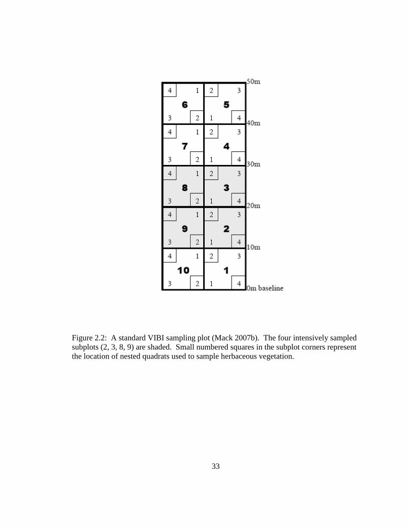
At each study area, a standard VIBI plot (Figure 2.2) was established. Each plot
was 20 meters wide by 50 meters long and divided using measuring tapes into 10-meter
by 10-meter subplots marked with stake flags. The compass bearing of the center line
was recorded and each plot corner was georeferenced using a Garmin 60 CSx handheld
GPS unit.
The percent cover of all plant species less than one meter tall was determined in
each of the four intensive subplots (2, 3, 8, and 9) (Figure 2.2). Any species encountered
in the six remaining subplots that did not occur in subplots 2, 3, 8, and 9 (i.e., new
species) was assigned a cover value based on the total area of the six subplots that were
not sampled intensively. Coverage was visually estimated using the following ten cover
classes: 1 (solitary/few), 2 (0-1% cover), 3 (1-2% cover), 4 (2-5% cover), 5 (5-10%
cover), 6 (10-25% cover), 7 (25-50% cover), 8 (50-75% cover), 9 (75-90% cover) and 10
(90-99% cover). Species level identification according to Voss (1971, 1985, 1996) was
recorded for most vascular plant species encountered. Mosses were identified only as
“bryophytes.” Any vascular plant that was not able to be confidently identified in the
field was collected, pressed, mounted on herbarium-grade paper and identified at a later
time. The complete methodology used to sample the vegetation in this study is described
in the Field Manual for the Vegetation Index of Biotic Integrity for Wetlands v1.4 (Mack
2007b).

15
Soil Data
A soil sample was taken to a depth of 12 cm, using a bucket auger, at the center of
each plot as stated in the VIBI field manual (Mack 2007b). The soil samples were placed
in bags, labeled and stored in a freezer until analyses could be conducted. The samples
were submitted to the Ohio State University’s Service Testing and Research (STAR)
Laboratory located at the Ohio Agricultural Research and Development Center (OARDC)
campus in Wooster, Ohio on October 30, 2009. Results of the analyses were received on
December 3, 2009. The samples were analyzed for soil reaction (pH), cation exchange
capacity (CEC), total phosphorus (P), total potassium (K), total calcium (Ca), total
magnesium (Mg), percent calcium (%Ca), percent magnesium (%Mg), percent potassium
(%K), percent nitrogen (%N), percent carbon (%C), and percent organic matter (%OM)
(STAR Lab 2011).
Physical Habitat Attributes
Physical habitat attribute data were collected in subplots 2, 3, 8 and 9. The
physical attributes recorded were: depth of standing surface water, litter depth, number of
tussocks, number of hummocks, number of macrotopographic depressions, a count of
coarse woody debris 12-40 cm in diameter, and a count of coarse woody debris greater
than 40 cm in diameter. Water and litter depth were determined using a measuring tape.

16
Plant Species Relative Cover Values
The relative cover of each plant species encountered in the sample plot was
calculated using an Excel spreadsheet designed specifically for VIBI data analysis (Mack
2007a). For each plot, the midpoints of the cover classes assigned to each species were
summed. Next, the total cover per species was summed to yield the total cover of all
species in the plot. Finally, the total cover of each species was divided by the total cover
of all species to yield the relative percent cover for each species. The formula used for
this calculation is:
Relative cover = ∑Ai / ∑Aij
where Ai = the cover class midpoints for a species, and Aij = the total cover of species Ai ,
Aj , etc. (Mack 2007b). A detailed description of the method used to calculate relative
cover is also provided in the VIBI field manual (Mack 2007b).
Statistical Analyses
Species richness, evenness (Pielou’s J) (Pielou 1969), Shannon-Weiner
index and Simpson’s index were calculated using the PC-ORD statistical software
program (McCune and Mefford 1999). Differences in the means of these diversity
measures between mitigation and reference plots were determined using Welch’s two-
sample t-test. A significance level of 0.05 was used to determine if differences between
groups were statistically significant.
In order to describe the similarity with respect to herbaceous plant communities,
an agglomerative hierarchical clustering technique based on a Euclidean dissimilarity

17
matrix was used to compare species cover values between mitigation and reference
forested wetland plots. Ward’s linkage method was used because of its compatibility
with Euclidean distances (McCune and Grace 2002). Cluster analysis is a useful way of
identifying groups when working with ecological data and has been used for many years
in community ecology (McCune and Grace 2002). The analysis was completed using the
PC-ORD statistical software program (McCune and Mefford 1999). The dendrogram
used to interpret the cluster analysis was scaled using Wishart’s (1969) objective function
which measures the amount of information lost at each step of the clustering procedure.
Multi-Response Permutation Procedure (MRPP) (Meilke and Berry 2001) was
used to test the null hypothesis of no significant differences between mitigation and
reference plots. A significance level of 0.05 was used to determine if the compositional
differences between groups were statistically significant. MRPP is a nonparametric
procedure that is useful for testing for significant differences between two or more
groups. It is an appropriate method to use with ecological community data that often do
not meet distributional assumptions required of parametric tests that address similar
questions (McCune and Grace 2002). Euclidean distance was used and groups were
defined based on classification as a mitigation plot or as a reference plot.
Nonmetric multidimensional scaling analysis (NMDS) was used to examine plant
community composition and species assemblages as they relate to physical environmental
attributes. NMDS is generally the most effective ordination method to use on ecological
data sets and its advantages include: (1) avoiding assumptions of linear relationships
among variables, (2) relieving the “zero truncation problem” associated with all

18
ordinations of community data sets, and (3) allowing the use of any distance measure or
relativation (McCune and Grace 2002). NMDS uses an iterative search to converge on a
solution that minimizes “stress” in the configuration. Stress is a function of a linear
monotone transformation of observed dissimilarities and ordination distances. The
NMDS procedure was performed using the VEGAN metaMDS function (Oksanen et al.
2010) in the R statistical computing program (R Development Core Team 2009). NMDS
allows for an indirect examination of how environmental factors may be influencing
community composition by fitting vectors representing environmental variables onto the
ordination using the envfit function (Oksanen et al. 2010).
Differences in soil chemical characteristics were examined using Mann-Whitney
nonparametric tests of group differences and a Welch two-sample t-tests were used to test
for significant group differences in physical habitat attributes. Methods of analysis were
chosen following Shapiro-Wilk tests for normality. A significance level of 0.05 was used
to evaluate if differences between groups were statistically significant.
Results
A total of 113 herbaceous species and genera were recorded in the sample plots
(Table 2.2). In mitigation plots, the most common herbaceous species based on mean
relative cover values included Lysimachia nummularia, Toxicodendron radicans, Bidens
frondosa, Lemna minor, Utricularia vulgaris and Carex lurida. The highest relative
covers in reference plots were recorded for Osmunda cinnamomea, moss spp., Osmunda
regalis and Glyceria striata. Welch’s two-sample t-tests indicated there were no

19
significant differences in species richness, evenness, Shannon-Wiener Index value or
Simpson diversity value between mitigation and reference plots (p > 0.05) (Figures 2.3
and 2.4).
Cluster Analysis
The cluster analysis dendrogram (Figure 2.5) shows that all four reference plots
were grouped together at distance 0.14 and before 15% percent of the available grouping
information was used. Trumbull Creek (TC) was grouped with the reference plots with
approximately 30% of the grouping information used. At distance 0.45 and with just
under 50% of the grouping information used, the Hale Road (HR) plot was added to the
group. The two remaining mitigation plots, Big Island (BI) and Columbia Station (CS),
were not grouped with the others until distance 0.94 and with almost 100% of the
grouping information used.
Multi Response Permutation Procedure
MRPP analysis indicated that there was a significant difference in herbaceous
species composition between mitigation and reference plots (p = 0.03). The chance-
corrected within group agreement (A), which is a description of the effect size that is
independent of the sample size, was 0.06. According to McCune and Grace (2002), A
values in community ecology are commonly below 0.1.
20
Nonmetric Multidimensional Scaling
Two convergent NMDS solutions were confirmed after three tries with a final
stress value of 5.98. Four of the environmental vectors that were fit to the ordination
(water depth, number of hummocks, number of tussocks, and number of
macrotopographic depressions) were statistically significant based on 999 permutations
of the data (p < 0.05) (Oksanen 2011). The vectors representing environmental gradients
(Figure 2.6) point in the direction of the most rapid change in each variable (Oksanen
2011).
The ordination plots depict site and species groupings (Figures 2.6 and 2.7).
Some species are grouped very closely near plot positions (Figures 2.6 and 2.7),
indicating that those species occurred either exclusively in particular plots or had very
high cover values relative to the corresponding values that were recorded for other plots.
For example, Trientalis borealis, Coptis trifolia, Rubus hispidus and Carex seorsa are all
very closely grouped near the position of Pallister State Nature Preserve (PA).
Additionally, Lysimachia nummularia, Apocynum cannabinum, Carex muskingumensis
and Asclepias incarnata are among species grouped near the position of the Big Island
(BI) mitigation plot. Species that occur in multiple plots and (or) have relatively
comparable cover values across different plots are located between plot locations in
ordination space. An example is Osmunda regalis which occurred commonly in both the
PA and Brown’s Lake Bog State Nature Preserve (BB) plots and is situated between the
two plot locations in ordination space (Figures 2.6 and 2.7).

21
All four reference plots and one mitigation plot (TC) were positively associated
with vectors representing the number of hummocks, number of tussocks, number of
macrotopographic depressions, litter depth, and counts of coarse woody debris greater
than 12 cm. (Figure 2.6). Three of the four mitigation plots were negatively associated
with these same vectors. One mitigation plot (HR) had a strong positive association with
water depth (Figure 2.6).
Soil Characteristics
The distributions of all soil characteristics were determined to be non-normal
using Shapiro-Wilk tests. Consequently, the mean value for each soil characteristic was
subjected to a Mann-Whitney nonparametric test of group differences. Mean values for
cation exchange capacity (p = 0.03) and total phosphorus (p = 0.03) were significantly
higher in the reference plots than in the mitigation plots (Table 2.3). There were no
significant differences found for any of the other soil characteristics.
Physical Habitat Attributes
The mean number of hummocks (p = 0.08), number of tussocks (p = 0.17),
number of macrotopographic depressions (p = 0.07), count of coarse woody debris > 40
cm in diameter (p = 0.19), litter depth (p = 0.23) and water depth (p = 0.39) were all
compared using Welch two-sample t-tests (Table 2.4). Only one attribute, the mean
count of coarse woody debris 12-40 cm in diameter, was significantly higher in reference
plots (p = 0.04).

22
Discussion
The results of this study highlight differences in the herbaceous plant community
composition of mitigation and reference forested wetlands in two ecoregions of Ohio and
revealed trends important for understanding wetland plant community development in
these ecoregions. MRPP analysis indicated that, overall, mitigation and reference plots
had significantly different herbaceous plant species compositions. Cluster analysis and
NMDS ordinations indicated a higher degree of similarity among reference plots than
among mitigation plots (Figures 2.5 and 2.6). Furthermore, ordination revealed several
tight species groupings which indicate that many species were unique to a single plot or
had a relatively high cover value in a particular plot (Figure 2.7). No significant
differences in species richness, evenness or diversity values were found, unlike the results
from other research comparing plant communities of non-forested natural and mitigation
wetlands (Balcombe et al. 2005). However, as noted by Mack (2009), forest subcanopies
tend to be low-energy systems compared with non-forested areas, therefore, significant
differences in diversity values may not be expected.
Physical Habitat Attributes
Many different factors may influence herbaceous plant community composition in
forest ecosystems including disturbance, physical factors (soil, microtopography),
biological processes (competition, colonization), and history (land use, successional age)
(Beatty 2003). In this study, we used the physical habitat attributes measured as part of
the VIBI protocol (Mack 2007b) as indicators of habitat complexity and
23
microtopographic heterogeneity. The importance of microtopography for plant
community development has been well-documented (Beatty 1984, Huenneke and Sharitz
1986, Titus 1990, Vivian-Smith 1997, Lee and Sturgess 2001, Anderson and Leopold
2002, Alsfeld et al. 2009, Duberstein and Conner 2009, Blood and Titus 2010).
In forested wetlands, there is often a wide variety of microsite types on the forest
floor including woody debris, tree trunks, litter- and moss-covered sediments and various
types of soil substrates (Ehrenfeld 1995). The presence and abundance of these
microsites has been shown to influence plant community development in forested
wetlands (Huenneke and Sharitz 1986, Blood and Titus 2010, Duberstein and Conner
2009). Consequently, microtopography has been a focus of several wetland restoration
projects (Rossell and Wells 1999, Bruland and Richardson 2005, Alsfeld et al. 2009,
Rossell et al. 2009).
The NMDS ordination revealed that all four undisturbed reference plots were
positively associated with hummocks, tussocks, macrotopographic depressions, coarse
woody debris and litter depth (Figure 2.6). These features were lacking in mitigation
plots (Figure 2.6, Table 2.4). This suggests that more mature, relatively undisturbed
forested wetlands may provide more microsites and therefore greater habitat complexity
which may favor the establishment and persistence of particular herbaceous plant species.
The physical attributes we measured may affect rates of litter accumulation, soil redox
potential, and soil moisture levels (Ehrenfeld 1995), and ultimately affect processes such
as seed accumulation, germination requirements and plant growth and mortality which
are critical to plant community development (Huenneke and Sharitz 1986). Some

24
physical habitat attributes may be critical for conservative plant species that have a
narrow range of ecological tolerances. Indeed, several ecologically conservative species
(e.g., Osmunda cinnamomea, Osmunda regalis, Glyceria septentrionalis) were associated
with physical habitat attributes that characterized reference plots (Figure 2.6) (Andreas et
al. 2004).
Past Land Use and Disturbance History
For both mitigation and reference plots, plant community composition and
physical habitat characteristics can be better understood by considering past land use and
disturbance history. Sampling for this study occurred in areas representing a range of
disturbance histories from relatively undisturbed areas to those recovering from recent
major disturbance (i.e., land clearing for agriculture). The BI and HR mitigation plots
were located in areas that were used for agricultural production just prior to wetland
restoration treatments (Envirotech Consultants, personal communication 2011; Vince
Messerly, personal communication 2011). Consequently, plant community development
in these areas has likely been affected by the lack of environmental heterogeneity that is
typical of post-agricultural landscapes (Beatty 2003, Flinn 2007).
Human-induced major disturbances often result in the removal of all native
vegetation and the elimination of the existing soil structure and microtopographic
features that are important for habitat heterogeneity. This reduction in environmental
heterogeneity and its effect on plant communities has been illustrated by the bryophyte
community compositions (Ross-Davis and Frego 2002) and fern recruitment (Flinn 2007)
25
found following human-induced disturbance. The development of microtopographic
features in heavily disturbed areas may only occur after a mature forest develops and then
experiences minor disturbances resulting in tree mortality and their eventual decay on the
forest floor. The resulting structure is a legacy of disturbance that lasts for hundreds of
years following the disturbance event itself (Lindenmayer and Franklin 2002, Beatty
2003). Furthermore, the formation of hummocks may require disturbance that creates
organically-derived structures (e.g., coarse woody debris and soil aggregates)
(Lindenmayer and Franklin 2002), followed by an accumulation of sediment and organic
material over the course of many years (Ehrenfeld 1995).
Several species adapted to full sun conditions (e.g., Scirpus cyperinus, Scirpus
atrovirens, Juncus effusus, Apocynum cannabinum, and Asclepias incarnata) (Mack
2007a) characterize the BI and HR mitigation plots (Figure 2.6 and 2.7). These species
may be biological legacies of the open, emergent or scrub-shrub wetlands that likely
occupied these plots in the relatively recent past. The presence of these early
successional species would be expected to decline over time as overall species diversity
changes in response to competition intensity, microclimate development, increases in
horizontal and vertical heterogeneity and sensitivity to disturbance (Gilliam and Roberts
2003). As these young forests transition from the stem exclusion stage to the understory
reinitiation stage of forest development (Oliver and Larson 1996), which takes several
decades, a herbaceous layer similar to those in the reference plots may begin to develop.
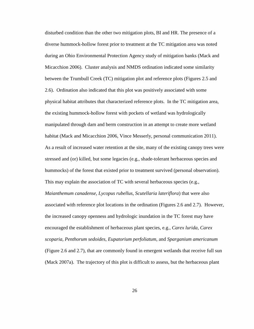
Two mitigation plots, TC and CS, were in mitigation areas with an existing,
relatively mature forest canopy at the time of treatment and may represent a less-
26
disturbed condition than the other two mitigation plots, BI and HR. The presence of a
diverse hummock-hollow forest prior to treatment at the TC mitigation area was noted
during an Ohio Environmental Protection Agency study of mitigation banks (Mack and
Micacchion 2006). Cluster analysis and NMDS ordination indicated some similarity
between the Trumbull Creek (TC) mitigation plot and reference plots (Figures 2.5 and
2.6). Ordination also indicated that this plot was positively associated with some
physical habitat attributes that characterized reference plots. In the TC mitigation area,
the existing hummock-hollow forest with pockets of wetland was hydrologically
manipulated through dam and berm construction in an attempt to create more wetland
habitat (Mack and Micacchion 2006, Vince Messerly, personal communication 2011).
As a result of increased water retention at the site, many of the existing canopy trees were
stressed and (or) killed, but some legacies (e.g., shade-tolerant herbaceous species and
hummocks) of the forest that existed prior to treatment survived (personal observation).
This may explain the association of TC with several herbaceous species (e.g.,
Maianthemum canadense, Lycopus rubellus, Scutellaria lateriflora) that were also
associated with reference plot locations in the ordination (Figures 2.6 and 2.7). However,
the increased canopy openness and hydrologic inundation in the TC forest may have
encouraged the establishment of herbaceous plant species, e.g., Carex lurida, Carex
scoparia, Penthorum sedoides, Eupatorium perfoliatum, and Sparganium americanum
(Figure 2.6 and 2.7), that are commonly found in emergent wetlands that receive full sun
(Mack 2007a). The trajectory of this plot is difficult to assess, but the herbaceous plant

27
community appears to be transitioning to one that is dominated by shade-intolerant
species.
Mack (2009) highlighted the difficulty in assessing forested wetland condition in
areas such as TC where disturbance affects the herbaceous plant community while the
canopy remains somewhat intact. Our result highlights the caution that must be used
when manipulating hydrology in mitigation wetlands and supports the conclusions of
other studies that found inundation to be greater in areas where hydrology was
manipulated for the purpose of creating wetlands (Cole et al. 2006, Gamble and Mitsch
2009). Additionally, our NMDS ordination indicated that the Hale Road (HR) plot was
highly associated with deeper water (Figure 2.6), and this result is corroborated by the
strong association of species that tolerate considerable inundation (e.g., Scirpus
atrovirens, Carex vulpinoidea, Lemna minor, Utricularia vulgaris) (personal
observation) with this plot (Figures 2.6 and 2.7). Our results further support the
suggestion that human manipulation of hydrology can have strong influences on the plant
community development of mitigation areas.
Neither cluster analysis nor NMDS ordination suggested that mitigation areas that
had a relatively mature canopy at the time of treatment were more similar to each other
than they were to young forested areas developing on post-agricultural land. Our results
illustrate considerable dissimilarity among mitigation areas and indicate that the
herbaceous understory communities of the young forests (BI and HR) were more similar
to mitigation plots with relatively mature trees (CS and TC) than they were to each other
(Figure 2.5).

28
The variability among mitigation plots may be suggestive of plant communities
that are adjusting to changing environmental conditions. The relatively similar
composition of reference plots (Figures 2.5 and 2.6) indicates that these forests are more
stable than those of mitigation plots. Also, ordination indicates that reference plots may
have well-established biological legacies (i.e., organically-derived structures
(Lindenmayer and Franklin 2002)) that may provide important habitat for some plant
species. These microsites may have provided the environmental conditions preferred by
ecologically conservative herbaceous understory plants (e.g., Carex bromoides, Carex
canescens, Carex tuckermanii, Dryopteris cristata, Coptis trifolia, Trientalis borealis)
(Andreas et al. 2004) that occurred exclusively in reference plots (Table 2.2).
Physiographic Factors and Landscape Position
It is likely that physiographic factors and landscape position affected the
herbaceous plant community composition of the sample plots. The TC mitigation plot
and PA reference plot were located in the northeasternmost county of Ohio (Ashtabula)
within the Mosquito Creek/Pymatuning Lowlands area of the EOLP ecoregion (Woods et
al. 1998). As a result of glacial influence, the Mosquito Creek/Pymatuning Lowlands
contain many areas with poorly drained soils that support relatively high numbers of
lakes, streams and wetlands (Woods et al. 1998). The poorly drained soils of this area
and its location in far northeastern Ohio, which is relatively cool and wet compared with
adjacent areas in the state, have encouraged the establishment of wetland plant species
that are more common in the Hemlock-White Pine-Northern Hardwoods Forest Region
29
than in the Beech-Maple Forest Region (Braun 1950, Andreas 1989). Notable
herbaceous species that occurred in these two plots and that are common in more
northern forests include: Maianthemum canadense, Dryopteris intermedia, Trientalis
borealis, Coptis trifolia, and Rubus hispidus (Figure 2.7). Also important is the observed
higher relative cover of moss, particularly Sphagnum spp. in these plots (personal
observation) which, as we suggested for vascular plants, may be related to the presence of
microtopographic features (Anderson et al. 2007) and physiographic factors.
The influence of physiographic conditions and landscape position was also
evident in the BB reference plot. This plot was located within the Low Lime Drift Plain
of the EOLP ecoregion characterized by scattered kettle lakes (Woods et al. 1998). The
sample plot itself was located in a depression near a kettle-hole bog (Brown’s Lake Bog
(The Nature Conservancy 2011)) and consequently supported many species associated
with “boggy forests” (e.g., Dryopteris cristata, Osmunda cinnamomea, Osmunda regalis,
Hydrocotyle americana, Circaea lutetiana) (Andreas 1989).
The CS mitigation plot was located in area of abandoned river channels (i.e.,
oxbows) associated with the West Branch of the Rocky River. It had relatively high
cover values for herbaceous species typically found in floodplains (e.g., Verbesina
alternifolia, Rudbeckia laciniata, Impatiens capensis) (Gordon 1969, Andreas 1989).
However, activities meant to restore hydrology in this area (i.e., ditch plugging and drain
tile destruction (Envirotech Consultants, personal communication 2011)) will presumably
influence the trajectory of the plant community. This hydrologic alteration will likely
encourage the establishment of herbaceous plant species adapted to more poorly drained

30
conditions rather than the well-drained conditions that characterize the soil map unit
associated with this plot (Table 2.1). The plant community may already be transitioning
given the association of shade-tolerant obligate wetland species such as Carex crinita var.
crinita and Glyceria striata with this plot (Figures 2.6 and 2.7).
Soil Characteristics
Soil samples from reference plots had significantly higher cation exchange
capacity and total phosphorus than those taken from mitigation plots; however, no
significant differences for any of the other soil characteristics were found. Other studies
have shown that soil properties vary among natural and mitigation wetlands (Moser et al.
2009). Furthermore, it has been suggested that microtopographic relief may also
influence soil properties in forested ecosystems (Beatty 1984, Ahn et al. 2009) and in
constructed depressional wetlands (Alsfeld et al. 2009). Since we collected a single soil
sample from the center of each plot, we were not able to investigate the variation in soil
characteristics in relation to plant community composition in these ecoregions. Given the
range of past land use intensity that characterized the mitigation plots in this study, future
investigations of soil characteristics at these sites may prove to be important for the
development of wetland mitigation techniques.
Conclusions
The techniques used to establish, restore and enhance forested wetlands result in
mitigation areas that represent a range of forest development stages that are inherently
31
different in their herbaceous plant community composition. This study suggests that
physical habitat attributes may influence herbaceous plant community development in
Ohio forested wetlands by providing a range of microsites that are available for plant
establishment. Mitigation areas may lack the microtopographic heterogeneity found in
relatively undisturbed forested wetlands and this feature can be attributed to past land
use, disturbance history, physiographic factors and landscape position. Furthermore,
wetland mitigation areas, particularly mitigation banks, are large, heterogeneous areas
that often support hundreds of acres of wetland in different stages of plant community
development. As forested wetlands currently used for mitigation continue to develop and
new mitigation projects are approved by regulatory agencies, more opportunities to study
herbaceous plant communities in these areas will arise. Nevertheless, our study provides
important insight into the current plant community development of some of Ohio’s
forested mitigation wetlands and represents a point from which additional research can be
conducted.

32
Figure 2.1: Locations of the four mitigation plots (black dots) and the four relatively undisturbed reference forested wetland plots (open circles).
33
Figure 2.2: A standard VIBI sampling plot (Mack 2007b). The four intensively sampled subplots (2, 3, 8, 9) are shaded. Small numbered squares in the subplot corners represent the location of nested quadrats used to sample herbaceous vegetation.

34
Figure 2.3: Mean diversity values (± 1 standard error) for herbaceous plant species in mitigation and reference forested wetland plots.
Figure 2.4: Mean species richness (± 1 standard error) for herbaceous plant species in mitigation and reference forested wetland plots.
mitigation reference
Spec
ies
Ric
hnes
s
0
10
20
30
40
50
mitigation reference0.0
0.5
1.0
1.5
2.0
2.5
3.0
Evenness (Pielou's J)Shannon-Weiner IndexSimpson's Index

Figure 2.5: Dendrogram from a hierarchical cluster analysis using herbaceous plant species relative cover values in mitigation (black dots) and reference (open circles) plots.
Reference Plots
35

Figure 2.6: Nonmetric multidimensional scaling (NMDS) ordination of mitigation plots (black dots) and reference plots (open circles). Environmental attributes represented by the vectors include: number of hummocks (# hummocks), number of tussocks (# tussocks), number of macrotopographic depressions (# macr. depr.), litter depth, water depth (H2O depth) and counts of coarse woody debris 12-40 cm in diameter (cwd 12-40 cm) and greater than 40 cm (cwd > 40 cm).
NMDS 1
-1.0 -0.8 -0.6 -0.4 -0.2 0.0 0.2 0.4 0.6 0.8
NM
DS
2
-1.0
-0.8
-0.6
-0.4
-0.2
0.0
0.2
0.4
0.6
mitigation reference
HR
TC
BI
CS
PA
BB
ACFW
H2O depth
# tussocks
litter depth
# macr. depr.
# hummocks
cwd >40 cm
cwd 12-40 cm
36

Figure 2.7: Nonmetric multidimensional scaling (NMDS) ordination of herbaceous plant species. Species abbreviations are provided in Table 2.2. Environmental attributes represented by the vectors include: number of hummocks (# hummocks), number of tussocks (# tussocks), number of macrotopographic depressions (# macr. depr.), litter depth, water depth (H2O depth) and counts of coarse woody debris 12-40 cm. in diameter (cwd 12-40 cm) and greater than 40 cm. (cwd > 40 cm).
NMDS 1
-1.0 -0.8 -0.6 -0.4 -0.2 0.0 0.2 0.4 0.6 0.8
NM
DS
2
-1.0
-0.8
-0.6
-0.4
-0.2
0.0
0.2
0.4
0.6
H2O depth
# tussocks
litter depth
# macr. depr.cwd >40
cwd 12-40
# hummocksEQUARVRUDLAC
VERALTCXAMPH
CICMACARIDRA
PLGPUN
CXGRAY ALLPETLYSCIL
THAPUB
ELYRIP
CINARUTOXRAD
APOCANLUDALTCXHYAL CXMUSK
ASCINC
RICNAT
LYSNUM
PARQUI
GEUCAN
PLGVIR
RANHISCIRLUT
LEEVIRAGRPAR
RICFLUCXSQUA
LEMMINCXVULP
SCICYPUTRVUL
VITRIPSCIATR
JUNEFF
ELEOBTALISUB
BIDCER
LYSTERPILPUM
IMPCAPCARSTI
CXCRINC
CXTRIB
BIDFRO
CXLUPL
GLYSTROSMCINDRYCRI
PANLAN PANCLA
SPIALB
HYDAMECXSWANCLEVIR
PILFON
SOLPATCXATLAA PLGCES
PHAARU
LEEORY PLGHYDGALTIN
LYCRUBSCULAT
MAICAN
PLGSAG
CXINTUCXGRAC
CXLURI
CXSCOP
POLPEN
LUDPAL ARITRI
PLGPERCUSGRO
HYPMUT
EUPPER
SPAAME
PENSEDTHENOV
CXSEOR
COPTRITRIBORSMIROT
RUBHISMITREP
LYCOBS
OSMREG
ONOSEN
DRYCAR
BIDCON
MOSS
BOECYL
GLYSEPJUNTEN
SANMAR
GALCIR
CXLUPFCRYCAN
OSMCLAEREHIE
GALAPACXBLAN
CXTUCK
CXBROM
SIUSUAAMBART
37

Table 2.1: Summary information describing the four mitigation plots and the four relatively undisturbed reference plots.
Plot name and
Symbol
Latitude Longitude Ecoregion Soil Map Unit Cowardin Classification
Plot Type Treatment Type
Alum Creek State Park
(AC)
40.20569
-82.94516
Eastern Corn Belt
Plains
Condit silt loam,
0-1 percent slopes (CnA)
palustrine, forested
reference
None
Brown’s Lake Bog SNP (BB)
40.68223 -82.06538 Erie/Ontario Drift and Lake
Plains
Carlisle muck (Ch)
palustrine, forested reference None
Fowler Woods SNP
(FW)
40.97188 -82.47080 Erie/Ontario Drift and Lake
Plains
Bennington silt loam, 0-2 percent
slopes (BnA)
palustrine, forested reference None
Pallister SNP (PA)
41.63452 -80.90465 Erie/Ontario Drift and Lake
Plains
Caneadea-Canadice silt
loam, 0-2 percent slopes (CeA)
palustrine, forested reference None
Big Island
(BI)
40.57825
-83.29400
Eastern Corn Belt
Plains
Latty silty clay
(La) and Paulding clay (Pa)
palustrine, forested
mitigation (bank)
hydrologic restoration
Columbia
Station (CS)
41.31612
-81.92192
Erie/Ontario
Drift and Lake Plains
Chagrin silt loam
(Ch)
palustrine, forested
mitigation
(consolidated)
hydrologic restoration
Hale Road
(HR)
41.28845
-82.16198
Erie/Ontario
Drift and Lake Plains
Mahoning silt
loam, 0-2 percent slopes (MgA)
palustrine, forested
mitigation (bank)
hydrologic restoration
Trumbull Creek (TC)
41.65917
-81.00477
Erie/Ontario Drift and Lake
Plains
Platea-Darien silt loams complex, 0-2 percent slopes
(PtA)
palustrine, forested
mitigation (bank)
hydrologic enhancement
38
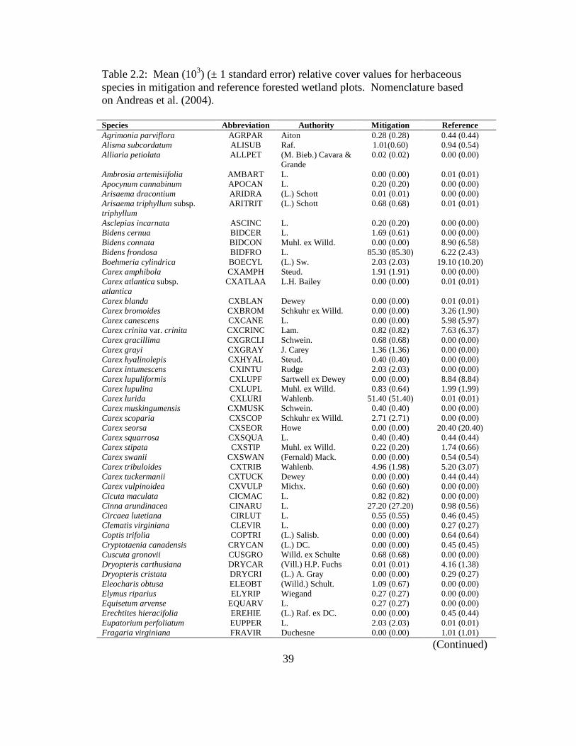
39
Table 2.2: Mean (103) (± 1 standard error) relative cover values for herbaceous species in mitigation and reference forested wetland plots. Nomenclature based on Andreas et al. (2004). Species Abbreviation Authority Mitigation Reference Agrimonia parviflora AGRPAR Aiton 0.28 (0.28) 0.44 (0.44) Alisma subcordatum ALISUB Raf. 1.01(0.60) 0.94 (0.54) Alliaria petiolata ALLPET (M. Bieb.) Cavara &
Grande 0.02 (0.02) 0.00 (0.00)
Ambrosia artemisiifolia AMBART L. 0.00 (0.00) 0.01 (0.01) Apocynum cannabinum APOCAN L. 0.20 (0.20) 0.00 (0.00) Arisaema dracontium ARIDRA (L.) Schott 0.01 (0.01) 0.00 (0.00) Arisaema triphyllum subsp. triphyllum
ARITRIT (L.) Schott 0.68 (0.68) 0.01 (0.01)
Asclepias incarnata ASCINC L. 0.20 (0.20) 0.00 (0.00) Bidens cernua BIDCER L. 1.69 (0.61) 0.00 (0.00) Bidens connata BIDCON Muhl. ex Willd. 0.00 (0.00) 8.90 (6.58) Bidens frondosa BIDFRO L. 85.30 (85.30) 6.22 (2.43) Boehmeria cylindrica BOECYL (L.) Sw. 2.03 (2.03) 19.10 (10.20) Carex amphibola CXAMPH Steud. 1.91 (1.91) 0.00 (0.00) Carex atlantica subsp. atlantica
CXATLAA L.H. Bailey 0.00 (0.00) 0.01 (0.01)
Carex blanda CXBLAN Dewey 0.00 (0.00) 0.01 (0.01) Carex bromoides CXBROM Schkuhr ex Willd. 0.00 (0.00) 3.26 (1.90) Carex canescens CXCANE L. 0.00 (0.00) 5.98 (5.97) Carex crinita var. crinita CXCRINC Lam. 0.82 (0.82) 7.63 (6.37) Carex gracillima CXGRCLI Schwein. 0.68 (0.68) 0.00 (0.00) Carex grayi CXGRAY J. Carey 1.36 (1.36) 0.00 (0.00) Carex hyalinolepis CXHYAL Steud. 0.40 (0.40) 0.00 (0.00) Carex intumescens CXINTU Rudge 2.03 (2.03) 0.00 (0.00) Carex lupuliformis CXLUPF Sartwell ex Dewey 0.00 (0.00) 8.84 (8.84) Carex lupulina CXLUPL Muhl. ex Willd. 0.83 (0.64) 1.99 (1.99) Carex lurida CXLURI Wahlenb. 51.40 (51.40) 0.01 (0.01) Carex muskingumensis CXMUSK Schwein. 0.40 (0.40) 0.00 (0.00) Carex scoparia CXSCOP Schkuhr ex Willd. 2.71 (2.71) 0.00 (0.00) Carex seorsa CXSEOR Howe 0.00 (0.00) 20.40 (20.40) Carex squarrosa CXSQUA L. 0.40 (0.40) 0.44 (0.44) Carex stipata CXSTIP Muhl. ex Willd. 0.22 (0.20) 1.74 (0.66) Carex swanii CXSWAN (Fernald) Mack. 0.00 (0.00) 0.54 (0.54) Carex tribuloides CXTRIB Wahlenb. 4.96 (1.98) 5.20 (3.07) Carex tuckermanii CXTUCK Dewey 0.00 (0.00) 0.44 (0.44) Carex vulpinoidea CXVULP Michx. 0.60 (0.60) 0.00 (0.00) Cicuta maculata CICMAC L. 0.82 (0.82) 0.00 (0.00) Cinna arundinacea CINARU L. 27.20 (27.20) 0.98 (0.56) Circaea lutetiana CIRLUT L. 0.55 (0.55) 0.46 (0.45) Clematis virginiana CLEVIR L. 0.00 (0.00) 0.27 (0.27) Coptis trifolia COPTRI (L.) Salisb. 0.00 (0.00) 0.64 (0.64) Cryptotaenia canadensis CRYCAN (L.) DC. 0.00 (0.00) 0.45 (0.45) Cuscuta gronovii CUSGRO Willd. ex Schulte 0.68 (0.68) 0.00 (0.00) Dryopteris carthusiana DRYCAR (Vill.) H.P. Fuchs 0.01 (0.01) 4.16 (1.38) Dryopteris cristata DRYCRI (L.) A. Gray 0.00 (0.00) 0.29 (0.27) Eleocharis obtusa ELEOBT (Willd.) Schult. 1.09 (0.67) 0.00 (0.00) Elymus riparius ELYRIP Wiegand 0.27 (0.27) 0.00 (0.00) Equisetum arvense EQUARV L. 0.27 (0.27) 0.00 (0.00) Erechtites hieracifolia EREHIE (L.) Raf. ex DC. 0.00 (0.00) 0.45 (0.44) Eupatorium perfoliatum EUPPER L. 2.03 (2.03) 0.01 (0.01) Fragaria virginiana FRAVIR Duchesne 0.00 (0.00) 1.01 (1.01) (Continued)

40
Table 2.2: Continued Galium aparine GALAPA L. 0.00 (0.00) 0.44 (0.44) Galium circaezans GALCIR Michx. 0.00 (0.00) 0.01 (0.01) Galium tinctorium GALTIN (L.) Scop. 4.37 (3.97) 3.43 (2.87) Geum canadense GEUCAN Jacq. 1.63 (1.63) 0.45 (0.44) Glyceria septentrionalis GLYSEP Hitchc. 0.00 (0.00) 14.20 (14.10) Glyceria striata GLYSTR (Lam.) Hitchc. 3.01 (1.99) 33.00 (27.70) Hydrocotyle americana HYDAME L. 0.00 (0.00) 1.61 (1.61) Hypericum mutilum HYPMUT L. 0.01 (0.01) 0.00 (0.00) Impatiens capensis IMPCAP Meerb. 5.44 (5.44) 25.70 (18.40) Juncus effusus JUNEFF L. 4.00 (3.16) 0.00 (0.00) Juncus tenuis JUNTEN Willd. 0.00 (0.00) 0.44 (0.44) Leersia oryzoides LEEORY (L.) Sw. 9.76 (7.64) 1.44 (0.95) Leersia virginica LEEVIR Willd. 2.90 (2.34) 2.39 (0.33) Lemna minor LEMMIN L. 75.40 (75.40) 1.57 (1.47) Ludwigia alternifolia LUDALT L. 0.61 (0.61) 0.00 (0.00) Ludwigia palustris LUDPAL (L.) Elliott 4.06 (4.06) 0.00 (0.00) Lycopodium obscurum LYCOBS L. 0.00 (0.00) 0.64 (0.64) Lycopus rubellus LYCRUB Moench 23.30 (22.90) 22.80 (8.06) Lysimachia ciliata LYSCIL L. 0.27 (0.27) 0.00 (0.00) Lysimachia nummularia LYSNUM L. 175.00 (129.00) 0.00 (0.00) Lysimachia terrestris LYSTER (L.) B.S.P. 0.54 (0.54) 2.49 (2.49) Maianthemum canadense MAICAN Desf. 2.71 (2.71) 2.56 (2.56) Mitchella repens MITREP L. 0.00 (0.00) 0.64 (0.64) Moss spp. MOSS N/A 20.10 (15.10) 91.30 (37.40) Onoclea sensibilis ONOSEN L. 4.06 (4.06) 3.71 (3.08) Osmorhiza claytonii OSMOCL (Michx.) C.B.
Clarke 0.00 (0.00) 0.44 (0.44)
Osmunda cinnamomea OSMCIN L. 0.00 (0.00) 101.00 (83.70) Osmunda regalis OSMREG L. 0.00 (0.00) 46.40 (30.40) Oxalis stricta OXASTR L. 0.00 (0.00) 0.50 (0.50) Panicum clandestinum PANCLA L. 0.00 (0.00) 0.27 (0.27) Panicum lanuginosum PANLAN Elliott 0.00 (0.00) 0.27 (0.27) Parthenocissus quinquefolia PARQUI (L.) Planch. 6.53 (6.53) 1.93 (0.74) Penthorum sedoides PENSED L. 2.88 (2.67) 0.00 (0.00) Phalaris arundinacea PHAARU L. 1.03 (0.59) 0.27 (0.27) Pilea fontana PILFON (Lunnell) Rydb. 0.00 (0.00) 0.01 (0.01) Pilea pumila PILPUM (L.) A. Gray 0.82 (0.82) 8.85 (7.18) Polygonum cespitosum PLGCES Blume 0.00 (0.00) 1.61 (1.61) Polygonum hydropiperoides PLGHPO Michx. 3.79 (3.27) 0.89 (0.89) Polygonum pensylvanicum PLGPEN L. 1.35 (1.35) 0.00 (0.00) Polygonum persicaria PLGPER L. 0.68 (0.68) 0.01 (0.01) Polygonum punctatum PLGPUN Elliott 0.27 (0.27) 0.00 (0.00) Polygonum sagittatum PLGSAG L. 0.68 (0.68) 0.28 (0.28) Polygonum virginianum PLGVIR L. 10.30 (10.30) 2.27 (1.67) Ranunculus hispidus RANHIS Michx. 0.54 (0.54) 0.44 (0.44) Riccia fluitans RICFLU L. 0.81 (0.81) 0.50 (0.50) Ricciocarpos natans RICNAT (L.) Corda 0.81 (0.81) 0.01 (0.01) Rubus hispidus RUBHIS L. 0.00 (0.00) 0.66 (0.66) Rudbeckia laciniata RUDLAC L. 0.01 (0.01) 0.00 (0.00) Sanicula marilandica SANIMA L. 0.00 (0.00) 0.88 (0.88) Scirpus atrovirens SCIATR Willd. 1.21 (1.21) 0.00 (0.00) Scirpus cyperinus SCICYP (L.) Kunth. 2.49 (1.71) 0.00 (0.00) Scutellaria lateriflora SCULAT L. 2.71 (2.71) 2.45 (1.88) Sium suave SIUSUA Walter 0.00 (0.00) 1.82 (1.25) Smilax rotundifolia SMXROT L. 0.00 (0.00) 0.64 (0.64) Solidago patula SOLPAT Muhl. ex Willd. 0.00 (0.00) 0.01 (0.01) Sparganium americanum SPAAME Nutt. 0.68 (0.68) 0.00 (0.00) (Continued)

41
Table 2.2: Continued Spiraea alba SPIALA Du Roi 0.00 (0.00) 0.27 (0.27) Thalictrum pubescens THAPUB Pursh 0.28 (0.28) 0.02 (0.02) Thelypteris noveboracensis THENOV (L.) Nieuwl. 0.68 (0.68) 0.00 (0.00) Toxicodendron radicans TOXRAD (L.) Kuntze 117.00 (113.00) 2.99 (0.98) Trientalis borealis TRIBOR Raf. 0.00 (0.00) 0.66 (0.66) Utricularia vulgaris UTRVUL L. 75.40 (75.40) 9.58 (9.58) Verbesina alternifolia VERALT (L.) Britton ex
Kearney 0.27 (0.27) 0.00 (0.00)
Vitis riparia VITRIP Michx. 0.16 (0.15) 0.00 (0.00)

42
Table 2.3: Mean values of (± 1 standard error) soil characteristics from mitigation and reference forested wetlands. An asterisk indicates a significant difference in the mean values between mitigation and reference sites (Mann-Whitney test; p < 0.05).
Soil Characteristic Mitigation Reference soil reaction (pH) 5.89 (0.41) 5.23 (0.13) total phosphorus (μg/g) 8.60 (0.93) 44.98 (29.96)* total potassium (μg/g) 165.76 (25.87) 179.62 (15.92) total calcium (μg/g) 2031.66 (462.50) 3793.69 (811.67) total magnesium (μg/g) 396.73 (68.47) 619.18 (82.09) cation exchange capacity 21.24 (2.36) 41.78 (6.58)* % calcium 51.08 (13.27) 44.00 (4.08) % magnesium 16.30 (0.39) 12.67 (1.41) % potassium 2.04 (0.27) 1.20 (0.25) % nitrogen 0.25 (0.04) 0.84 (0.45) % carbon 2.40 (0.61) 10.47 (6.31) % organic matter 4.85 (0.10) 23.85 (13.46)
Table 2.4: Mean values (± 1 standard error) of physical attributes from mitigation and reference forested wetland plots. An asterisk indicates a significant difference in the mean values between mitigation and reference sites (Welch two-sample t-test; * p < 0.05).
Attribute Mitigation Reference Depth of standing water 0.31 (0.31) 0.00 (0.00) Litter depth 0.57 (0.26) 1.25 (0.43) Number of tussocks 0.44 (0.36) 1.13 (0.24) Number of hummocks 0.81 (0.81) 3.69 (1.08) Number of macrotopographic depressions 2.25 (0.53) 3.75 (0.40) Coarse woody debris 12-40 cm diameter 0.19 (0.19) 4.81 (1.36)* Coarse woody debris >40 cm diameter 0.00 (0.00) 0.75 (0.45)

43
REFERENCES
Ahn, C., P.M. Gillevet, M. Sikaroodi and K.L. Wolf. 2009. An assessment of soil bacterial community structure and physicochemistry in two microtopographic locations of a palustrine forested wetland. Wetlands Ecology and Management 17:397-407.
Alsfeld, A.J., J.L. Bowman and A. Deller-Jacobs. 2009. Effects of woody debris, microtopography, and organic matter amendments on the biotic community of constructed depressional wetlands. Biological Conservation 142:247-255.
Anderson, H.M., R.G. Margaret, M.F. Jurgensen and C.C. Trettin. 2007. Vascular and non-vascular plant community response to silvicultural practices and resultant microtopography creation in a forested wetland. Wetlands 27:68-79.
Anderson, K.L. and D.J. Leopold. 2002. The role of canopy gaps in maintaining vascular plant diversity at a forested wetland in New York State. Journal of the Torrey Botanical Society 129:238-250.
Andreas, B. K.1989. The Vascular Flora of the Glaciated Allegheny Plateau Region of Ohio. Bulletin of the Ohio Biological Survey, Volume 8, Number 1. The Ohio State University, Columbus, Ohio.
Andreas, B. K., J. J. Mack and J. S. McCormac. 2004. Floristic quality assessment index (FQAI) for vascular plants and mosses for the state of Ohio. Ohio Environmental Protection Agency, Division of Surface Water, Wetland Ecology Group, Columbus, Ohio.
Balcombe, C.K., J.T. Anderson, R.H. Fortney, J.S. Rentch, W.N. Grafton and W.S. Kordek. 2005. A comparison of plant communities in mitigation and reference wetlands in the mid-Appalachians. Wetlands 25:130-142.
Battaglia, L.L., P.R. Minchin and D.W. Pritchett. 2002. Sixteen years of old-field succession and reestablishment of a bottomland hardwood forest in the Lower Mississippi Alluvial Valley. Wetlands 22:1-17.
Beatty, S.W. 1984. Influence of microtopography and canopy species on spatial patterns of forest understory plants. Ecology 65:1406-1419.
44
Beatty, S.W. 2003. Habitat heterogeneity and maintenance of species in understory communities. In: Gilliam, F. S. and M. R. Roberts (eds.). The Herbaceous Layer in Forests of Eastern North America. Oxford University Press, New York.
Blood, L.E. and J.H. Titus. 2010. Microsite effects on forest regeneration in a bottomland swamp in western New York. Journal of the Torrey Botanical Society 137:88-102.
Braun, E. L. 1950. Deciduous Forests of Eastern North America. Hafner Publishing Company Inc., New York.
Braun, E. L. 1961. The Woody Plants of Ohio. Ohio State University Press, Columbus, Ohio.
Brinson, M. M. 1993. A hydrogeomorphic classification for wetlands. U.S. Army Corps of Engineers Waterways Experiment Station. Wetlands Research Program Technical Report. WRP-DE-4.
Brinson, M.M. and R. Rheinhardt. 1996. The role of reference wetlands in functional assessment and mitigation. Ecological Applications 6:69-76.
Brown, S.C. and P.L.M. Veneman. 2001. Effectiveness of compensatory wetland mitigation in Massachusetts, USA. Wetlands 21:508-518.
Bruland, G.L. and C.J. Richardson. 2005. Hydrologic, edaphic, and vegetative responses to microtopographic reestablishment in a restored wetland. Restoration Ecology 13:515-523.
Cole, C.A. and D. Shafer. 2002. Section 404 wetland mitigation and permit success criteria in Pennsylvania, USA, 1986-1999. Environmental Management 30:508-515.
Cole, C.A., C.A. Urban, P. Russo, J. Murray, D. Hoyt and R.P. Brooks. 2006. Comparison of long-term water levels of created and natural reference wetlands in northern New York, USA. Ecological Engineering 27:166-172.
Cowardin, L. M., V. Carter, F. C. Golet and E. T. LaRoe. 1979. Classification of wetlands and deepwater habitats of the United States. Department of the Interior, Fish and Wildlife Service, Washington D.C.
Dahl, T. E. 1990. Wetland Losses in the United States, 1780's to 1980's. United States Department of the Interior, Fish and Wildlife Service, Washington D.C.
Duberstein, J.A. and W.H. Conner. 2009. Use of hummocks and hollows by trees in tidal freshwater forested wetlands along the Savannah River. Forest Ecology and Management 258:1613-1618.

45
Ehrenfeld, J.G. 1995. Microsite differences in surface substrate characteristics in Chamaecyparis swamps of the New Jersey Pinelands. Wetlands 15:183-189.
Envirotech Consultants. 2011. Personal communication.
Flinn, K.M. 2007. Microsite-limited recruitment controls fern colonization of post-agricultural forests. Ecology 88:3103-3114.
Gamble, D.L. and W.J. Mitsch. 2009. Hydroperiods of created and natural vernal pools in central Ohio: a comparison of depth and duration of inundation. Wetlands Ecology and Management 17:385-395.
Gilliam, F. S. and M. R. Roberts (Eds.). 2003. The Herbaceous Layer in Forests of Eastern North America. Oxford University Press, New York.
Gordon, R. B. 1969. Natural Vegetation of Ohio in Pioneer Days. The Ohio State University, Columbus, Ohio.
Hoeltje, S.M. and C.A. Cole. 2007. Losing function through wetland mitigation in central Pennsylvania, USA. Environmental Management 39:385-402.
Huenneke, L.F. and R.R. Sharitz. 1986. Microsite abundance and distribution of woody seedlings in a South-Carolina cypress-tupelo swamp. American Midland Naturalist 115:328-335.
Kettlewell, C.I., V. Bouchard, D. Porej, M. Micacchion, J.J. Mack, D. White and L. Fay. 2008. An assessment of wetland impacts and compensatory mitigation in the Cuyahoga River Watershed, Ohio, USA. Wetlands 28:57-67.
Kruse, B.S. and J.W. Groninger. 2003. Vegetative characteristics of recently reforested bottomlands in the lower Cache River watershed, Illinois, USA. Restoration Ecology 11:273-280.
Lee, P. and K. Sturgess. 2001. The effects of logs, stumps, and root throws on understory communities within 28-year-old aspen-dominated boreal forests. Canadian Journal of Botany 79:905-916.
Lindenmayer, D. B. and J. F. Franklin . 2002. Conserving Forest Biodiversity: A Comprehensive Multiscaled Approach. Island Press, Washington D.C.
Mack, J. J. 2004. Integrated wetland assessment program, part 4: vegetation index of biotic integrity (VIBI) and tiered aquatic life uses (TALUs) for Ohio wetlands. Ohio EPA Technical Report WET/2004-4. Ohio Environmental Protection Agency, Wetland Ecology Group, Division of Surface Water, Columbus, Ohio.
46
Mack, J. J. and M. Micacchion. 2006. An ecological assessment of Ohio mitigation banks: vegetation, amphibians, hydrology, and soils. Ohio EPA Technical Report WET/2006-1. Ohio Environmental Protection Agency, Division of Surface, Wetland Ecology Group, Columbus, Ohio.
Mack, J. J. 2007a. Automated spreadsheets for calculating and reporting the vegetation index of biotic integrity (VIBI) metrics and scores v. 1.0.1. Ohio Environmental Protection Agency, Wetland Ecology Group, Division of Surface Water, Columbus, Ohio.
Mack, J. J. 2007b. Integrated wetland assessment program, part 9: field manual for the vegetation index of biotic integrity for wetlands v. 1.4. Ohio EPA Technical Report WET/2007-6. Ohio Environmental Protection Agency, Wetland Ecology Group, Division of Surface Water, Columbus, Ohio.
Mack, J.J. 2009. Development issues in extending plant-based IBIs to forested wetlands in the Midwestern United States. Wetlands Ecology and Management 17:117-130.
McCune, B. and J. B. Grace . 2002. Analysis of Ecological Communities. MJM Software, Gleneden Beach, Oregon.
McCune, B. and M.J Mefford. 2006. PC-ORD. Multivariate analysis of ecological data. Version 5. MjM Software, Glenedon Beach, Oregon.
Messerly, V. 2011. Personal communication.
Mielke Paul W., J. and K. J. Berry. 2001. Permutation Methods: A Distance Function Approach. Springer Series in Statistics, New York, New York.
Mitsch, W. J. and J. G. Gosselink . 2007. Wetlands, 4th edition. John Wiley and Sons, New York, New York.
Moser, K.F., C. Ahn and G.B. Noe. 2009. The influence of microtopography on soil nutrients in created mitigation wetlands. Restoration Ecology 17:641-651.
National Research Council . 2001. Compensating for Wetland Losses Under the Clean Water Act. National Academy Press, Washington D.C.
Niswander, S.F. and W.J. Mitsch. 1995. Functional analysis of a 2-year-old created in-stream wetland: Hydrology, phosphorus retention, and vegetation survival and growth. Wetlands 15:212-225.

47
Ohio Department of Natural Resources. 2010. Rare Native Ohio Plants 2010-2011 Status List. Available online at http://www.ohiodnr.com/Home/Rare_Plants/20102011RareNativeOhioPlants/tabid/22557/Default.aspx. Accessed April 16, 2011.
Okland, R.H., K. Rydgren and T. Okland. 2008. Species richness in boreal swamp forests of SE Norway: The role of surface microtopography. Journal of Vegetation Science 19:67-74.
Oksanen, J., F. G. Blanchet, R. Kindt, P. Legendre, R. G. Ohara, G. L. Simpson, M. H. H. Stevens and H. Wagner 2010. vegan: Community ecology package. R package version 1.17-0. Available online at: http://CRAN.R-project.org/package=vegan. Accessed April 16, 2011.
Oliver, C.D. and Larson, B.C. 1996. Forest Stand Dynamics, Update Edition. John Wiley and Sons, Inc., New York.
Peet, R.K., T.R. Wentworth and P.S. White. 1998. A flexible, multipurpose method for recording vegetation composition and structure. Castanea 63:262-274.
Pfingston, R.A. 1998. Distribution of Ohio amphibians. In: Lanoo, M.J. (Ed.). Status and Conservation of Midwestern Amphibians. University of Iowa Press, Iowa City, Iowa.
Pielou, E. C. 1969. An Introduction to Mathematical Ecology. John Wiley and Sons, New York, New York.
Porej, D. 2003. Faunal aspects of wetland restoration. Ph.D. Dissertation. The Ohio State University, Columbus, Ohio.
Porej, D., M. Micacchion and T.E. Hetherington. 2004. Core terrestrial habitat for conservation of local populations of salamanders and wood frogs in agricultural landscapes. Biological Conservation 120:399-409.
R Development Core Team. 2009. R: a language and environment for statistical computing. R Foundation for Statistical Computing, Vienna, Austria. ISBN 3-900051-07-0. Available online AT: http://www.R-project.org. Accessed April 16, 2011.
Ross-Davis, A.L. and K.A. Frego. 2002. Comparison of plantations and naturally regenerated clearcuts in the Acadian Forest: forest floor bryophyte community and habitat features. Canadian Journal of Botany 80:21-33.

48
Rossell, I.M. and C.L. Wells. 1999. The seed banks of a southern Appalachian fen and an adjacent degraded wetland. Wetlands 19:365-371.
Rossell, I.M., K.K. Moorhead, H. Alvarado and Warren, Robert J., II. 2009. Succession of a southern Appalachian mountain wetland six years following hydrologic and microtopographic restoration. Restoration Ecology 17:205-214.
Soil Survey Staff, Natural Resources Conservation Service, United States Department of Agriculture. Soil survey geographic (SSURGO) database for Ashtabula, Delaware, Lorain, Marion, Richland and Wayne Counties, Ohio. Available online at http://soildatamart.nrcs.usda.gov. Accessed April 16, 2011.
Spieles, D.J. 2005. Vegetation development in created, restored, and enhanced mitigation wetland banks of the United States. Wetlands 25:51-63.
Spieles, D.J., M. Coneybeer and J. Horn 2006. Community structure and quality after 10 years in two central Ohio mitigation bank wetlands. Environmental Management 38:837-852.
The Nature Conservancy. 2011. Brown's Lake Bog Preserve. Available online at http://www.nature.org/ourinitiatives/regions/northamerica/unitedstates/ohio/placesweprotect/browns-lake-bog-preserve.xml. Accessed April 16, 2011.
The Ohio Agricultural Research and Development Center, Service Testing and Research Laboratory (STAR Lab). 2011. Methods and References. Available online at: http://oardc.osu.edu/starlab/references.asp. Accessed April 16, 2011.
Titus, H.J. 1990. Microtopography and woody plant regeneration in a hardwood floodplain swamp in Florida. Bulletin of the Torrey Botanical Club 117:429-437.
U.S. Army Corps of Engineers (USACE) and U.S. Environmental Protection Agency (USEPA). 2008. Compensatory Mitigation for Losses of Aquatic Resources; Final Rule. Federal Register 73.
Vivian-Smith, G. 1997. Microtopographic heterogeneity and floristic diversity in experimental wetland communities. Journal of Ecology 85: 71-82.
Voss, E. G.1996. Michigan Flora: a guide to the identification and occurrence of the native and naturalized seed-plants of the state, Part III, Dicots (Pyrolaceae - Compositae). Cranbrook Institute of Science Bulletin 61 and University of Michigan Herbarium, Ann Arbor, Michigan.

49
Voss, E. G.1985. Michigan Flora: a guide to the identification and occurrence of the native and naturalized seed-plants of the state, Part II, Dicots (Saururaceae - Cornaceae). Cranbrook Institute of Science Bulletin 59 and University of Michigan Herbarium, Ann Arbor, Michigan.
Voss, E. G. 1972. Michigan Flora: a guide to the identification and occurrence of the native and naturalized seed-plants of the state, Part I, Gymnosperms and Monocots. Cranbrook Institute of Science Bulletin 55 and University of Michigan Herbarium, Bloomfield Hills, Michigan.
Wishart, D. 1969. An algorithm for hierarchical classifications. Biometrics 25:165-170.
Woods, A. J., J. M. Omernik, C. S. Brockman, T. D. Gerber, W. D. Hosteter and S. H. Azevedo. 1998. Ecoregions of Indiana and Ohio, 1:1500000. Available at http://www.epa.gov/wed/pages/ecoregions/ohin_eco.htm. Accessed May 28, 2011.

50
CHAPTER 3
WOODY PLANT COMMUNITY COMPOSITION AND STRUCTURE OF
FORESTED MITIGATION WETLANDS AND RELATIVELY UNDISTURBED
REFERENCE FORESTED WETLANDS
Abstract
Compensatory mitigation for impacts to forested wetlands is a topic that has
generated considerable debate among scientists and regulators in recent years. There is
considerable uncertainty associated with the development of desirable woody plant
communities in forested mitigation areas, which is critical to the overall biological
integrity of forested wetlands. We examined woody plant community characteristics and
physical habitat attributes of four forested mitigation wetlands and four relatively
undisturbed reference forested wetlands within the Erie/Ontario Drift and Lake Plains
and Eastern Corn Belt Plains ecoregions of Ohio. Within the study areas we sampled
woody vegetation and physical habitat attributes using protocols established by the Ohio
Environmental Protection Agency for wetland assessment. Our objective was to compare
the woody plant community composition and structure of mitigation and reference
forested wetlands and identify factors that may be influencing woody plant community
development in these areas. Multi-response permutation procedure (MRPP) indicated
that woody plant composition was not significantly different between

51
mitigation and reference plots (p = 0.11). The compositions of both reference and
mitigation plots concurred with the general description of elm-ash-maple forests in Ohio.
Dominant canopy tree species in both plot types were Ulmus americana, Fraxinus
pennsylvanica, Acer saccharinum and Acer rubrum. However, our data suggests that
relatively undisturbed forests supported higher numbers of ecologically-conservative
species and species adapted to certain environmental conditions (e.g., shade and saturated
soil). Nonmetric multidimensional scaling (NMDS) ordination revealed that reference
plots were positively associated with several physical habitat attributes, e.g., hummocks,
macrotopographic depressions and coarse woody debris which were also associated with
several ecologically conservative species. Structurally, the density of wetland shrub
species (p = 0.02) and importance of native woody subcanopy species (p = 0.03) were
both significantly higher in reference plots than in mitigation plots. Activities meant to
restore, establish or enhance forested wetlands for use as compensatory mitigation result
in forests representing a range of disturbance histories and development stages. The
woody plant community characteristics of these mitigation areas are likely influenced by
several variables including disturbance history, physiographic factors and landscape
position. At a more local scale, physical habitat attributes such as hummocks,
macrotopographic depressions and coarse woody debris provide important microsites that
encourage the establishment and persistence of some woody species in forested
mitigation wetlands.
52
Introduction
Woody plants (i.e., trees, shrubs and vines) are important components of forested
wetland ecosystems. This structure is characterized by the physical and temporal
distribution of woody plants (Oliver and Larson 1996), and is closely associated with the
species composition at any given time during forest stand development. Understanding
the factors that influence woody plant community composition and structure can provide
insight into the capacity of a forested wetland to provide important ecological functions
(e.g., water quality enhancement and habitat for flora and fauna). The unique
hydroperiods and plant community structure of forested wetlands are important for
certain bird species (Kaminski et al. 1993, Riffell et al. 2006, Hoover 2009, Benson and
Bednarz 2010), amphibian species (Baldwin et al. 2006, Karraker and Gibbs 2009),
invertebrate species (Braccia and Batzer 2001, Batzer et al. 2005) and rare plant species
(Laidig et al. 2009, Scanga and Leopold 2010). Unfortunately, forested wetlands are
very difficult to restore, establish and (or) enhance (National Research Council 2003,
Mitsch and Gosselink 2007). Yet in Ohio, forested wetlands continue to be negatively
impacted at rates equal to or higher than those for other wetland types (Porej 2003).
Prior to European settlement, forested wetlands were common within the
deciduous forest that covered most of Ohio (Braun 1961, Gordon 1969, Andreas 1989).
Within the Beech-Maple Forest Region of Ohio, Braun (1961) describes extensive tracts
of elm-ash-maple forest that occupied depressions and intermorainal flats. Following
European settlement of the state, much of the forest including forested wetlands was
cleared to harvest timber, to make the land suitable for agriculture (Gordon 1969), and

53
later, for commercial and residential developments. In addition, environmental attributes
such as soil structure, hydrologic regime and microtopographic heterogeneity were
drastically altered by draining and plowing areas that were too wet for agriculture and
urban development.
The ecological value of undisturbed forested wetlands has been increasingly
realized and understanding the factors influencing forested wetland restoration is now a
priority for scientists (Schoenholtz et al. 2001, Allen et al. 2004). During the design of
wetland restoration, establishment and enhancement projects (i.e., wetland mitigation)
(USACE and USEPA 2008) meant to replace wetland functions following disturbance,
much attention is given to the establishment of woody plant communities similar to those
that characterize natural, undisturbed forested wetlands. To identify factors that may be
influencing forested wetland mitigation development, we investigated woody plant
community composition and structure in mitigation forested wetlands and relatively
undisturbed reference forested wetlands in Ohio. The relatively undisturbed areas
represent reference standards that are important for mitigation wetland assessment
(Brinson and Rheinhardt 1996). Specifically, the objectives of this chapter are to: 1)
compare the woody plant community composition and structure of forested mitigation
wetlands and relatively undisturbed reference forested wetlands, and 2) identify factors
that may be influencing the woody plant community composition and structure in both
types of forested wetlands.

54
Study Areas
A total of eight study areas (Figure 3.1, Table 3.1) were located within the
Erie/Ontario Drift and Lake Plains (EOLP) and Eastern Corn Belt Plains (ECBP)
ecoregions of Ohio (Woods et al. 1998). The study areas were confined to these
ecoregions to reduce the effect of major climatic and physiographic differences compared
with adjacent ecoregions. Both ecoregions fall within the Beech-Maple Forest Region
described by Braun (1950). The Wisconsinan glacial deposits of this region support a
variety of lakes, streams and wetlands, and forested wetland plant communities in the
region are typically dominated by the following canopy tree species and genera:
American elm (Ulmus americana), ash (Fraxinus spp.), silver maple (Acer saccharinum),
and red maple (Acer rubrum) (Braun 1950,1961, Gordon 1969, Andreas 1989).
Four study areas identified as representing relatively undisturbed reference
forested wetlands were randomly selected from a database provided by the Ohio
Environmental Protection Agency’s Wetland Ecology Group. The four reference plots
were located in low-lying natural depressions. The four randomly selected mitigation
areas were in relatively flat areas or depressions where the restoration, establishment and
(or) enhancement (USACE and USEPA 2008) of forested wetlands had occurred. All
eight study plots were located in areas classified as palustrine forested wetlands
according to the Classification of Wetlands and Deepwater Habitats of the United States
(Cowardin et al. 1979).
Three of the mitigation plots were located within approved mitigation banks and
the fourth was within a “consolidated” mitigation area that includes several individual

55
mitigation projects constructed according to Clean Water Act, Section 404 permits.
Banks are different from consolidated areas because they are large areas where wetland
restoration, establishment, enhancement and in some cases preservation activities are
planned and approved by the Interagency Review Team before being used for any
specific compensatory mitigation (USACE and USEPA 2008). Once approved, bank
credits become available to anyone needing to purchase mitigation acreage to compensate
for permitted wetland impacts. Currently, mitigation banks are the preferred mitigation
option of federal regulatory agencies (USACE and USEPA 2008).
Physiography and Soils
Six of the sample plots were located in the EOLP ecoregion that is characterized
as an area with a variety of lakes, streams and wetlands in locations where the land is flat
and soils are clayey (Woods et al. 1998). More specifically, two sample plots (Pallister
SNP and Trumbull Creek) were located in the Mosquito Creek/Pymatuning Lowlands
sub-ecoregion that is characterized by poorly drained soils and wet-mesic forests (Woods
et al. 1998). The other four EOLP plots (Brown’s Lake Bog SNP, Columbia Station,
Fowler Woods SNP and Hale Road) were located in the Low Lime Drift Plain sub-
ecoregion that is characterized by low rolling hills and end moraines with scattered kettle
lakes (Woods et al. 1998). The soil map units associated with the sampling locations
(Table 3.1) in the EOLP are in a range of drainage classes from very poorly drained to
well-drained (Soil Survey Staff 2011).

56
Two sample plots and were located in the Eastern Corn Belt Plains (ECBP)
ecoregion that is characterized as a rolling till plain with local end moraines (Woods et al.
1998). One ECBP plot (Alum Creek State Park) was within the Loamy, High Lime Till
Plains sub-ecoregion which contains soils that developed from loamy, limy Wisconsinan
glacial deposits. The other ECBP plot (Big Island) was within the Clayey, High Lime
Till Plains sub-ecoregion with soils that contain more clay content than the adjacent
Loamy, High Lime Till Plains. The soil map units associated with these two sample plots
(Table 3.1) are described as somewhat poorly drained or very poorly drained (Soil Survey
Staff 2011).
Methods
Vegetation Data
With the objective of comparing woody plant community composition and
structure at forested wetland mitigation areas in Ohio, it was important to use methods
that have been previously applied for mitigation project evaluation (Mack and
Micacchion 2006, Micacchion and Gara 2008, Micacchion et al. 2010). To allow for
direct comparison, the Vegetation Index of Biotic Integrity for Wetlands v1.4 (VIBI), a
vegetation-based wetland assessment tool developed by Mack (2007b) was used to
characterize woody plant communities. All vegetation data were collected between June
15 and September 15, 2009. The VIBI sampling method is based on the releve method
for vegetation sampling described by Peet et al. (1998).

57
At each study area, a standard VIBI plot (Figure 3.2) was established. Each plot
was 20 meters wide by 50 meters long and divided using measuring tapes into 10-meter
by 10-meter subplots marked with stake flags. The compass bearing of the center line
was recorded and each plot corner was georeferenced using a Garmin 60 CSx handheld
GPS unit.
In each of the ten subplots, species-level identification according to Braun (1961)
was recorded for every woody plant greater than one meter tall. Any woody plant that
was not able to be confidently identified in the field was collected, pressed, mounted on
herbarium-grade paper and identified at a later time. The diameter at breast height (dbh)
was taken at a height of 1.37 meters for each individual woody plant with the exception
of multi-stemmed shrubs (e.g., Cephalanthus occidentalis) which were classified as
“shrub clumps.” The dbh measurement of each woody plant that was not a multi-
stemmed shrub was placed in one of the following classes: 1 (0 - < 1cm), 2 (1 - <2.5 cm),
3 (2.5 - <5 cm), 4 (5 - <10 cm), 5 (10 - <15 cm), 6 (15 - <20 cm), 7 (20 - <25 cm), 8 (25 -
<30 cm), 9 (30 - <35 cm) and 10 (35 - <40 cm). Any dbh measurement greater than 40
cm was recorded individually to the nearest tenth of a centimeter. The complete
methodology used to sample the woody vegetation in this study is described in the Field
Manual for the Vegetation Index of Biotic Integrity for Wetlands v1.4 (Mack 2007b).
Soil data
A soil sample was taken to a depth of 12 cm, using a bucket auger, at the center of
each plot as stated in the VIBI field manual (Mack 2007b). The soil samples were placed

58
in bags, labeled and stored in a freezer until analyses could be conducted. The samples
were submitted to the Ohio State University’s Service Testing and Research (STAR)
Laboratory located at the Ohio Agricultural Research and Development Center (OARDC)
campus in Wooster, Ohio on October 30, 2009. Results of the analyses were received on
December 3, 2009. The samples were analyzed for soil reaction (pH), cation exchange
capacity (CEC), total phosphorus (P), total potassium (K), total calcium (Ca), total
magnesium (Mg), percent calcium (%Ca), percent magnesium (%Mg), percent potassium
(%K), percent nitrogen (%N), percent carbon (%C), and percent organic matter (% OM)
(STAR Lab 2011).
Physical Habitat Attributes
Physical habitat attribute data were collected in subplots 2, 3, 8 and 9. The
physical attributes recorded were: depth of standing water, litter depth, number of
tussocks, number of hummocks, number of macrotopographic depressions, a count of
coarse woody debris 12-40 cm in diameter, and a count of coarse woody debris greater
than 40 cm in diameter. Water depth and litter depth were determined using a measuring
tape.
Vegetation Data Reduction and Metric Calculations
To calculate species importance values (the average of the relative frequency,
relative density and relative dominance of a species) and VIBI metric values, a series of
data reductions were necessary as outlined in the VIBI field manual (Mack 2007b). For

59
calculations that consider only wetland species, the wetland indicator statuses according
to the National List of Plant Species That Occur in Wetlands (Reed 1988) were used to
separate wetland species from non-wetland species. Those statuses are: obligate wetland
(OBL), facultative wetland (FACW), facultative (FAC), facultative upland (FACU) and
obligate upland (UPL) (Reed 1988). To calculate the density of wetland shrubs and
wetland trees, only species with a FACW or OBL indicator status were used in the
calculation (Mack 2007a). Data reduction calculations were completed using a Microsoft
Excel spreadsheet created by OEPA specifically for VIBI data analysis (Mack 2007a).
Statistical Analyses
Species richness, evenness (Pielou’s J) (Pielou 1969), Shannon-Weiner
index values and Simpson diversity values were calculated using the PC-ORD statistical
software program (McCune and Mefford 2006). Differences in the means of these
diversity measures between mitigation and reference plots were determined using
Welch’s two-sample t-test. A significance level of 0.05 was used to evaluate if
differences between groups were statistically significant.
To characterize woody plant community structure, differences in mean density
(number of stems per hectare) of wetland tree species (i.e., species coded as “native
wetland tree” by Mack (2007a)) and mean importance value of canopy tree species (i.e.,
those that would occupy the upper canopy at maturity (Mack 2007b, 2009)) (Table 3.2)
between mitigation and reference plots were evaluated using Mann-Whitney
nonparametric tests for group differences. Additionally, Welch two-sample t-tests were

60
used to evaluate differences in mean density (number of shrub clumps per hectare) of
wetland shrub species and subcanopy IV metric values (Table 3.2). Shapiro-Wilk tests
for normality were used to determine the appropriate tests for significant group
differences in these structural measures between mitigation and reference plots. A
significance level of 0.05 was used to evaluate if differences between groups were
statistically significant.
In order to describe the similarity with respect to woody plant community
composition, an agglomerative hierarchical clustering technique based on a Euclidean
dissimilarity matrix was used to compare the woody plant species importance values
between mitigation and reference forested wetland plots. Ward’s linkage method was
used because of its compatibility with Euclidean distances (McCune and Grace 2002).
Cluster analysis is a useful way of identifying groups when working with ecological data
and has been used for many years in community ecology (McCune and Grace 2002). The
analysis was completed using the PC-ORD statistical software program (McCune and
Mefford 2006). The dendrogram used to interpret the cluster analysis was scaled using
Wishart’s (1969) objective function which measures the amount of information lost at
each step of the clustering procedure.
Multi-Response Permutation Procedure (MRPP) (Meilke and Berry 2001) was
used to test for a significant difference in woody plant species composition between
mitigation and reference plots. MRPP is a nonparametric procedure that is useful for
testing for a significant difference between two or more groups. It is an appropriate
method to use with ecological community data that often do not meet distributional
61
assumptions required of parametric tests that address similar questions (McCune and
Grace 2002). Euclidean distance was used and groups were defined based on
classification as a mitigation plot or as a reference plot. Statistical significance of the
results was evaluated using a significance level of 0.05.
Nonmetric multidimensional scaling analysis (NMDS) was used to examine
woody plant community compositions as they relate to physical habitat attributes.
NMDS is an effective ordination method to use on ecological data sets and its advantages
include: (1) avoiding assumptions of linear relationships among variables, (2) relieving
the “zero truncation problem” associated with all ordinations of community data sets, and
(3) allowing the use of any distance measure or relativation (McCune and Grace 2002).
NMDS uses an iterative search to converge on a solution that minimizes “stress” in the
configuration. Stress is a function of a linear monotone transformation of observed
dissimilarities and ordination distances. The NMDS procedure was performed using the
VEGAN metaMDS function (Oksanen et al. 2010) in the R statistical computing program
(R Development Core Team 2009). NMDS allows for an indirect examination of how
environmental factors may be influencing community composition by fitting vectors
representing environmental variables onto the ordination using the envfit function
(Oksanen et al. 2010).
Differences in soil chemical characteristics were examined using Mann-Whitney
nonparametric tests of group differences, and Welch two-sample t-tests were used to test
for significant group differences in physical habitat attributes. Methods of analysis were

62
chosen following Shapiro-Wilk tests for normality. A significance level of 0.05 was used
to evaluate if differences between groups were statistically significant.
Results
A total of forty-eight woody plant species greater than one meter tall were found
in the sample plots (Table 3.3). The results from Welch’s two-sample t-tests indicated
that there were no significant differences in species richness, evenness (Pielou’s J),
Shannon-Wiener index values or Simpson diversity values between mitigation and
reference plots (p > 0.05) (Figures 3.2 and 3.3). In mitigation plots, the most important
species were Fraxinus pennsylvanica, Acer saccharinum, Acer rubrum and Ulmus
americana. The highest mean importance values in reference plots were calculated for
Acer saccharinum, Acer rubrum, Ulmus americana, Nyssa sylvatica, Cephalanthus
occidentalis and Quercus bicolor. Standing dead trees had high mean importance values
in both mitigation and reference plots. The tests for group differences in structural
measures found a significantly higher density of wetland shrub species (p = 0.02) (Figure
3.4) and significantly higher mean subcanopy IV metric value at mitigation sites (p =
0.03) (Figure 3.5), but no significant difference for mean density of wetland trees (p =
0.20) or mean canopy IV metric values (p = 0.12) (Figures 3.6 and 3.7). Two mitigation
plots had considerably higher stem densities in smaller diameter classes than the other six
plots (Table 3.4).

63
Cluster Analysis
Two reference plots, Fowler Woods (FW) and Alum Creek (AC) grouped
together very early in the clustering procedure at distance 0.063. At distance 0.13, two
mitigation plots, Big Island (BI) and Hale Road (HR) grouped together. Trumbull Creek
(TC) grouped with Pallister State Nature Preserve (PA) at distance 0.24 followed by the
grouping of Columbia Station (CS) with FW and AC at distance 0.38, and Brown’s Lake
Bog (BB) was added to that group at 0.56. Finally, BI and HR were grouped with CS,
FW, and AC at distance 1.20 and TC and PA were added at 2.03 to complete the
dendrogram (Figure 3.8).
Multi Response Permutation Procedure
MRPP indicated that there was no significant difference in woody plant species
composition between mitigation and reference plots (p = 0.11). The chance-corrected
within group agreement (A), which is a description of the effect size that is independent
of the sample size, was 0.07. A values in community ecology are commonly below 0.1
(McCune and Grace 2002).
Nonmetric Multidimensional Scaling
NMDS analysis of woody plant importance values converged on a stable solution
after five tries with a final stress value of 3.53. The ordination diagram depicts the
relationships among the sample plots and species, and provides an indirect examination
of physical habitat attribute influences using vectors (Figure 3.9). The number of
64
tussocks and depth of litter were both strongly associated with NMDS axis 1. Coarse
woody debris 12-40 cm in diameter and greater than 40 cm in diameter were associated
with NMDS axis 2. The number of hummocks, number of macrotopographic depressions
and water depth were associated with both axes.
The ordination plot depicts plot and species groupings (Figure 3.9). Some species
are grouped very closely near plot positions, indicating that those species occurred either
exclusively in particular plots or had high importance values relative to the corresponding
values that were recorded for other plots. For example, Betula alleghaniensis, Carpinus
caroliniana, Fraxinus nigra and Pinus strobus are species grouped very closely near the
PA plot position. Also, Acer negundo, Platanus occidentalis, Quercus macrocarpa, and
Viburnum lentago are species that are strongly associated with the CS plot in ordination
space. Species that occur in multiple plots and (or) have comparable importance values
across several plots are located between plot locations in ordination space. An example
is Ulmus americana, an important species in several plots that is not strongly associated
with any single plot position in ordination space.
Soil Characteristics
The distributions of all the soil characteristics were determined to be non-normal
using Shapiro-Wilk tests. Consequently, the mean values for soil characteristics were
subjected to Mann-Whitney nonparametric tests for group differences. Mean values for
cation exchange capacity (CEC) (p = 0.03) and total phosphorus (P) (p = 0.03) were
significantly higher for reference plots than for mitigation plots (Table3.5).

65
Physical Habitat Attributes
The mean number of hummocks (p = 0.08), number of tussocks (p = 0.17),
number of macrotopographic depressions (p = 0.07), count of coarse woody debris > 40
cm in diameter (p = 0.19), litter depth (p = 0.23) and water depth (p = 0.39) were all
compared using Welch two-sample t-tests (Table 2.4). Only one attribute, the mean
count of coarse woody debris 12-40 cm in diameter, was significantly higher in reference
plots (p = 0.04).
Discussion
Canopy Composition
The composition of canopy tree species (i.e., those that would occupy the upper
canopy at maturity (Mack 2007b, 2009)) in all plots concurred with the general
description of the elm-ash-maple forests known to occur in Ohio (Braun 1950, 1961;
Gordon 1969, Andreas 1989). Dominant canopy tree species in both plot types were
Ulmus americana, Fraxinus pennsylvanica, Acer saccharinum and Acer rubrum. Given
the low number of tree species that occurred in the sample plots, MRPP results did not
indicate a significant compositional difference between mitigation and reference plots.
When the most important canopy species in each plot were used for interpretation,
cluster analysis revealed three distinct groups (Figure 3.8). Two young mitigation plots,
BI and HR, in the stem exclusion stage of forest development (Oliver and Larson 1996)
were very similar and were characterized by the dominance of one species, Fraxinus
pennsylvanica (Figure 3.8). This is not surprising given the lightweight seeds of this

66
species and its documented dominance of restored, 5 to 7 year old forested wetlands
(Kruse and Groninger 2003, Ruzicka et al. 2010) and disturbed forested wetlands in Ohio
(Mack 2004). Acer rubrum and Acer saccharinum characterized the canopies of the
reference plots as well as the TC and CS mitigation plots which both had existing,
relatively mature canopies prior to restoration or enhancement treatment (Figure 3.8).
Acer spp. may be important components of more mature forested wetlands and may
become more important in the BI and HR plots during later stages of forest development.
Diversity index values were similar for the two plot types (Figures 3.2 and 3.3);
however, several canopy species that are considered to be ecologically-conservative
(Andreas et al. 2004) were strongly associated with reference plots (Figure 3.9). Those
species include: Quercus bicolor, Quercus rubra, Quercus alba, Nyssa sylvatica,
Fraxinus nigra, Fraxinus profunda, Betula alleghaniensis and Pinus strobus (Table 3.3).
Only one conservative canopy species, Quercus macrocarpa, occurred in mitigation plots
but not reference plots (Table 3.3).
NMDS ordination indicates that conservative canopy species in reference plots
may be associated with physical habitat attributes that increase microtopographic
heterogeneity (Figure 3.9). The establishment of canopy species that prefer upland
habitats (e.g., Quercus rubra, Quercus alba, Fagus grandifolia, Liriodendron tulipifera)
(Reed 1988) may have been encouraged by the greater abundance of elevated microsites
such as hummocks, tussocks and coarse woody debris that characterized the reference
plots (Table 3.6). Conservative wetland species (e.g., Quercus bicolor, Nyssa sylvatica)

67
which can tolerate saturated soil conditions, may prefer the range of hydrologic
conditions offered by the more microtopographically diverse reference plots.
Physiographic factors and landscape position were likely very important in
shaping the canopy composition of some plots. The PA reference plot and TC mitigation
plot were more similar to each other than to other plots as indicated by the cluster
dendrogram (Figure 3.8), and both were located in the Mosquito Creek/Pymatuning
Lowlands described by Woods et al. (1998) as a poorly drained area containing many
wetlands. This sub-ecoregion extends into the far northeastern part of Ohio, where Braun
(1950, 1961) describes a transition zone within the Beech-Maple Forest Region where
species typically found in the Hemlock-White Pine-Northern Hardwoods Forest Region
become more common. NMDS ordination shows that species associated with the
Hemlock-White Pine-Northern Hardwoods Forest Region (e.g., Betula alleghaniensis,
Pinus strobus) were strongly associated with the PA plot (Figure 3.9). Also, the
dominance of Acer rubrum in the PA and TC plots (Figure 3.8) is not surprising given the
importance of this species in forests of northeastern Ohio where soils tend to be poorly
drained (Widmann et al. 2009).
Landscape position was likely very important for the canopy development of the
CS mitigation plot. This plot was located in an area of abandoned river channels (i.e.,
oxbows) associated with the West Branch of the Rocky River. Consequently, species
typically associated with floodplains (e.g., Acer negundo, Platanus occidentalis and
Populus deltoides (Braun 1961, Gordon 1969, Andreas 1989)) were associated with this
plot (Figure 3.9). Drain tile destruction and ditch plugging characterized the restoration

68
treatment in this area (Envirotech consultants, personal communication 2011). As a
result of increased soil saturation and (or) inundation, the floodplain species associated
with this plot may be replaced with species that can tolerate poorly drained soil
conditions.
Canopy Structure
Although not statistically significant, mitigation plots had a higher mean stem
density of wetland trees than reference plots (Figure 3.6). This was primarily driven by
the high stem densities of the BI and HR plots (Table 3.4) that are in the stem exclusion
stage of forest development. It is very important to consider that the canopy structure of
these two plots may change drastically within the next several years. Mortality of
Fraxinus pennsylvanica, which dominates these two plots, is expected to increase
throughout Ohio due to emerald ash borer (Agrilus planipennis) infestation (Widmann et
al. 2009). As a result, forested wetlands dominated by Fraxinus pennsylvanica may
develop large canopy openings (i.e., gaps) which will have implications for both
overstory and understory plant community development in these areas.
The TC and CS mitigation plots supported canopy tree species in a broader range
of diameter classes than the BI and HR plots (Table 3.4), which is suggestive of the
understory reinitiation development stage and greater structural complexity (Oliver and
Larson 1996). This trend highlights one advantage of restoring, establishing or
enhancing wetlands in areas that are already forested: desired vertical structure may
already exist. However, manipulating areas that already support mature trees can have

69
negative effects on the long-term development of forested wetlands. This has been well-
documented in studies of “greentree reservoirs” in the Lower Mississippi Alluvial Valley
(LMAV). The impoundment of bottomland hardwood forests in the LMAV has been
shown to affect forest composition, tree mortality and recruitment (King et al. 1998,
Ervin et al. 2006).
In this study, we were able to identify some structural characteristics of the
sampled areas based on tree stem densities and the distributions of stems among diameter
classes. However, a more in-depth analysis of canopy structure that considers crown
dimensions and the relative positions of tree crowns in the canopy is needed to fully
understand how the canopies of mitigation and reference forested wetlands compare to
one another.
Subcanopy Composition
The subcanopy communities of the reference plots were generally dominated by
shrub and small tree species considered to be ecologically conservative, e.g., Vaccinium
corymbosum, Ilex verticillata, Amelanchier arborea, Hamamelis virginiana and
Cephalanthus occidentalis (Andreas et al. 2004). Subcanopy species composition in the
mitigation plots was characterized by the presence and relative importance of non-native
and invasive species (e.g., Rhamnus frangula and Rosa multiflora) and species that are
not shade-tolerant (e.g., Cornus amomum, Rosa palustris) (Mack 2007a) (Figure 3.9,
Table 3.3). Differences in disturbance history and forest development stage may partly
explain these compositional differences.

70
During the stem exclusion phase of forest development very few plants are able to
successfully establish in the understory (Peet and Christensen 1987, Oliver and Larson
1996). This exclusion of new understory plants may be responsible for the absence of
shade-tolerant shrub and small tree species in the BI and HR plots, and indicates that
shrub species persisting in these plots represent biological legacies of the early
successional emergent or scrub-shrub wetland communities that once occupied the
sampled areas. Furthermore, certain physical habitat attributes (e.g., coarse woody debris
and hummocks) that may favor the establishment of some woody species by creating
elevated microsites (Huenneke and Sharitz 1986, Titus 1990, Blood and Titus 2010) are
lacking in the BI and HR plots (Figure 3.9). Physical habitat attributes that are legacies
of disturbance may not develop in these forests until the canopy trees mature, die and fall
to the forest floor (Lindenmayer and Franklin 2002).
Several shade-tolerant and shade-facultative wetland shrub species (e.g., Ilex
verticillata, Cephalanthus occidentalis, Lindera benzoin, Vaccinium corymbosum) were
strongly associated with reference plots (Figure 3.9). In addition, ecologically
conservative species (e.g., Ilex verticillata, Cephalanthus occidentalis, Vaccinium
corymbosum, Amelanchier arborea, Hamamelis virginiana) (Andreas et al. 2004) were
also associated with reference plots (Figure 3.9). Our ordination suggests that the
presence of certain physical habitat attributes may be partly responsible for the
establishment and persistence of these shrub species (Figure 3.9). The processes through
which physical habitat attributes may promote woody plant establishment are discussed
later in this chapter.

71
As we suggested for the canopy tree composition, landscape position may have
influenced subcanopy species composition. The BB reference plot was located near a
kettle-hole bog (Brown’s Lake Bog (The Nature Conservancy 2011)) and Vaccinium
corymbosum, a dominant shrub of bogs in Ohio (Andreas 1989), was an important
species in this plot. It is likely that this species was able to persist in the sampled area
following canopy closure over what was once an open bog community. Vaccinium
corymbosum is known to occur in the understory of swamp forests of northeastern Ohio
(Braun 1961).
Although mitigation plots generally lacked hummocks, tussocks, coarse woody
debris and had shallower litter layers (Table 3.6), the TC mitigation plot was positively
associated with some of these features (Figure 3.9). The presence of these features in the
TC plot may represent a legacy of the mature hummock-hollow forest that characterized
this area prior to hydrologic enhancement (Mack and Micacchion 2006), and helps
explain the presence of Hamamelis virginiana, a conservative shrub species that occurred
exclusively on remnant hummocks in this plot (personal observation).
Subcanopy Structure
Our results indicate that reference forested wetlands had a significantly higher
density of wetland shrub species and significantly higher subcanopy species importance
values (IV) than mitigation areas (Figures 3.4 and 3.5). The density of wetland shrubs
reflects the abundance of native shrub species with a facultative wetland or obligate
wetland (Reed 1988) indicator status. The subcanopy IV metric is a measure of the

72
importance of native shrub or small tree species that tolerate at least partial shade
regardless of their wetland indicator status (Table 3.2) (Mack 2007b, 2009). Both of
these measures were significantly higher in reference plots indicating that they have more
complex vertical and horizontal subcanopy structure than mitigation plots. Shrub species
that characterize mitigation plot subcanopies (e.g., Cornus amomum, Rosa palustris,
Rosa multiflora) (Figure 3.9) may not survive in these forests due to either intolerance of
shade or a preference for drier habitats (Reed 1988, Mack 2007a).
The lower density of shade-tolerant wetland shrubs in mitigation plots can be
better understood by considering disturbance history and forest development stage. Two
mitigation plots, BI and HR, are young forests developing on post-agricultural land and
are still in the stem exclusion stage of development which is characterized by self-
thinning and a lack of new woody plant establishment in the understory (Peet and
Christensen 1987, Oliver and Larson 1996). The young dense canopies of these plots
likely have not experienced gap-forming disturbances that temporarily increase available
light and encourage the establishment and growth of woody understory plants (Peet and
Christensen 1987). In young even-aged forests, canopy gaps resulting from tree mortality
are quickly occupied by expansion of the crowns of neighboring trees (Oliver and Larson
1996). Even in the absence of canopy gaps, the lack of light penetration through the
young dense canopy may discourage woody subcanopy species establishment which has
been strongly correlated with increased light levels (Van Pelt and Franklin 2000).
Minor disturbances also often leave structural legacies (i.e., pits, mounds and
coarse woody debris) (Lindenmayer and Franklin 2002) on the forest floor. These

73
legacies influence environmental conditions such as the spatial variability of hydrologic
conditions, and soil nutrient and soil oxygen heterogeneity which affect plant growth and
establishment (Vivian-Smith 1997, Neatrour et al. 2005, 2007). Furthermore, elevated
microsites associated with physical legacies may provide “safe sites” or “windows of
opportunity” that allow shrub and small tree species to become established (Huenneke
and Sharitz 1986, Jordan and Hartman 1995, Eriksson and Froborg 1996). Although
first-year woody plant seedlings have been found to be most abundant in wet depressions
in forested wetlands (Blood and Titus 2010), flooding may ultimately inhibit their
survivorship and growth (Kozlowski 1984, Anderson et al. 2009), and seedlings that
survive longer than one year likely established on elevated microsites (Titus 1990, Blood
and Titus 2010).
Following establishment, the presence of some shrub species in deeply shaded
forest understories may be maintained through vegetative reproduction rather than sexual
reproduction (Kanno and Seiwa 2004, Matlaga and Horvitz 2009). Vegetative
reproduction presumably favors shrub species in forests because new stems are able to
rely on stored carbohydrates from their parents until gap formation allows rapid growth
in the presence of increased light (Kanno and Seiwa 2004). Additionally, the physical
connection to parent plants prevents stems from being easily uprooted by flooding
disturbance (Huenneke and Sharitz 1986).
In this study, many native shade-tolerant and shade-facultative shrub and small
tree species were associated with physical habitat attributes that characterized the
reference plots (Figure 3.9). This suggests that certain habitat characteristics of relatively
74
undisturbed forested wetlands may promote the establishment of native subcanopy
species that will be long-term structural components due to their tolerance of shaded
conditions. This is consistent with other research that investigated understory vegetation
as it relates to forest maturity, structural complexity and microhabitat heterogeneity
(D’Amato et al. 2009). Many of the shrub species associated with mitigation plots (e.g.,
Cornus amomum, Rosa palustris, Rubus allegheniensis) are shade-intolerant species that
represent biological legacies of the open emergent or scrub-shrub wetland communities
that likely occupied these sites prior to canopy closure. These species would not be
expected to persist as forest development progresses.
Barring any major disturbance, the subcanopy strata of the CS and TC mitigation
plots may begin to resemble those of the reference plots sooner than BI and HR given
their more advanced development stage. The stem exclusion stage that characterized the
young BI and HR plots may last for several decades before a stratum of shade-tolerant
shrubs becomes established (Oliver and Larson 1996). The forests of CS and TC will
likely be influenced by minor disturbances in the near future that create gaps and leave
physical legacies that encourage the establishment of native, shade-tolerant shrub and
small tree species. NMDS ordination indicated that the TC plot may already have some
physical habitat attributes similar to those of the reference plots (Figure 3.9). However,
the manipulation of hydrology (i.e., dam and berm construction) in the TC mitigation
area which has already caused canopy tree mortality and encouraged the dominance of
species adapted to full sun conditions (Chapter 2), may inhibit the establishment of
shade-tolerant subcanopy species for many years.

75
Standing Dead Trees
Standing dead trees were important structural components of both the mitigation
plots and the reference plots. However, the processes responsible for tree mortality may
differ between the plot types. The standing dead trees in the BI and HR mitigation plots
were likely casualties of the intense competition for canopy space that characterizes self-
thinning and the stem exclusion development stage (Peet and Christensen 1987, Oliver
and Larson 1996). Tree mortality in the reference plots may be more influenced by
disturbance (e.g., windthrow, impacts from falling trees, and disease) which have been
documented as important causes of tree mortality in mature forests (Larson and Franklin
2010). Natural processes may also have contributed to the presence of standing dead
trees in the TC and CS mitigation plots that had existing, relatively mature canopies at the
time of treatment. However, the aforementioned hydrologic disturbance in the TC plot is
likely responsible for the high importance of standing dead trees in that plot which was
highlighted in an Ohio EPA study of wetland mitigation banks (Mack and Micacchion
2006). Additionally, increased water retention resulting from hydrologic manipulation in
the CS mitigation area (Envirotech Consultants, personal communication 2011) may have
contributed to the deaths of some trees adapted to the well-drained conditions that
characterize the soil map unit in that area (Soil Survey Staff 2011) (Table 3.1). It is
difficult to predict the long-term response of canopy trees in the CS mitigation plot to the
hydrologic manipulation. Certainly, any area with a mature canopy that is subjected to
hydrologic manipulation should be monitored closely.
76
Soil Characteristics
Soil characteristics likely play a role in shaping woody plant communities in the
sample plots. Soils in the reference plots have a significantly higher mean cation
exchange capacity and total phosphorus than those of mitigation plots, but no significant
differences were found in any of the other soil characteristics. Other researchers have
shown that soil properties vary among natural and mitigation wetlands (Moser et al.
2009), and that microtopographic relief may influence soil properties in forested
ecosystems (Beatty 1984, Ahn et al. 2009) and plant community development in
constructed depressional wetlands (Alsfeld et al. 2009). Since we collected a single soil
sample from each plot, we were not able to investigate the role soil characteristics may
have in shaping woody plant community composition especially as it relates to
microtopographic variation. Future studies of the effects of microtopographic
heterogeneity on soil characteristics in forested wetlands are needed to fully understand
the role soils play in shaping woody plant communities in Ohio’s forested mitigation
wetlands.
Conclusions
The results of this study indicate that both relatively undisturbed forested
wetlands and mitigation forested wetlands in northern Ohio are dominated by species that
characterize the elm-ash-maple forests known to occur in the state. However, a closer
examination reveals that young mitigation plots were characterized by the dominance of
Fraxinus pennsylvanica while more mature mitigation areas and reference plots had
77
canopies dominated by Acer spp. As the young forests mature, Acer spp. may become
more important in the canopies of these areas.
The undisturbed conditions of reference forested wetlands may provide more
suitable habitat for some ecologically conservative tree and shrub species that are adapted
to wet, shaded conditions. Our analyses suggest that the diversity of physical habitat
attributes that characterized reference plots in this study may be important for the
establishment of these conservative woody plants. We suggest that the development of
physical habitat features that increase microtopographic heterogeneity should be
incorporated into future forested mitigation wetland designs.
The techniques currently used to restore, establish and enhance forested wetlands
for the purpose of mitigation have resulted in forests representing a range of disturbance
histories and developmental stages with inherently different structural characteristics.
Although mitigation plots sampled for this study did support some shrub species, many of
these species are more typical of open, emergent or scrub-shrub wetlands than forested
wetland subcanopies. Structural complexity associated with native, shade-tolerant
wetland subcanopy species may not develop in mitigation wetlands for several decades.
The result may be a temporal shift in forested wetland structure across Ohio’s landscape.
As forested wetlands currently used for mitigation develop and new mitigation projects
are approved by regulatory agencies, more opportunities to study woody plant
community development in these areas will arise. Nevertheless, our study provides
important insight into the current status of plant community development of Ohio’s

78
forested mitigation wetlands and represents a point from which research can be
continued.

79
Figure 3.1: Locations of the four forested wetland mitigation plots (black dots) and the four relatively undisturbed reference forested wetland plots (open circles).

80
Figure 3.2: Mean (± 1 standard error) diversity values for woody plant species of mitigation and reference forested wetland plots.
Figure 3.3: Mean (± 1 standard error) species richness for woody plant species of mitigation and reference forested wetland plot
mitigation reference0.0
0.5
1.0
1.5
2.0
2.5
3.0
Evenness (Pielou's J)Shannon-Wiener IndexSimpson's Index
mitigation reference
Spec
ies
Ric
hnes
s
0
5
10
15
20
25

81
mitigation reference
Num
ber o
f wet
land
shr
ubs
per h
ecta
re
0
200
400
600
800
1000
Figure 3.4: Mean (± 1 standard error) density of wetland shrubs (number per hectare) of mitigation and reference plots. There was a significant difference between plot types (Welch two-sample t-test, p = 0.02).
Figure 3.5: Mean (± 1 standard error) subcanopy IV metric value of mitigation and reference plots. There was a significant difference between plot types (Welch two-sample t-test, p = 0.03).
mitigation reference
Subc
anop
y IV
met
ric v
alue
0.00
0.02
0.04
0.06
0.08
0.10
0.12
0.14
0.16
0.18

82
Figure 3.6: Mean (± 1 standard error) density of wetland trees (stems per hectare) of mitigation and reference plots. There was no significant difference between plot types (Welch two-sample t-test, p = 0.20).
Figure 3.7: Mean (± 1 standard error) canopy species IV metric value in mitigation and reference plots. There was no significant difference between plot types (Welch two-sample t-test, p = 0.12).
mitigation reference
Num
ber o
f wet
land
tree
s pe
r hec
tare
0
2000
4000
6000
8000
10000
mitigation reference
Cano
py IV
met
ric v
alue
0.00
0.05
0.10
0.15
0.20
0.25
0.30

Figure 3.8: Dendrogram from a hierarchical cluster analysis using woody plant species importance values from mitigation plots (black dots) and reference plots (open circles). The most important canopy tree species in each plot was added to the dendrogram to aid interpretation of the results.
Acer saccharinum
Fraxinus pennsylvanica
Acer rubrum
83

Figure 3.9: Nonmetric multidimensional scaling (NMDS) ordination of mitigation plots (black dots), reference plots (circles) and woody plant species (triangles). Species abbreviations are provided in Table 3.3. Environmental attributes represented by the vectors include: number of hummocks (# hummocks), number of tussocks (# tussocks), number of macrotopographic depressions (# macr. depr.), litter depth, water depth (H2O depth) and counts of coarse woody debris 12-40 cm in diameter (cwd 12-40) and greater than 40 cm (cwd > 40).
NMDS 1
-1.0 -0.5 0.0 0.5 1.0 1.5
NM
DS
2
-1.5
-1.0
-0.5
0.0
0.5
1.0
1.5
speciesmitigation reference
PRUSER
QUEIMB
ILEVER
VACCOR
QUERUB
ACERUBNYSSYL
FAGGRA
FRANIGPINSTR
QUEALBSMIROTHAMVIR CRPCAR
BETALLAMEARB
STADEA
CAROVT
FRAPROLIRTUL
LINBENTOXRAD
VIBREC
CEPOCC
QUEBICULMAME
ACESACCARLACPARQUI
ROSMUL
ACENEGQUEMACVIBLEN
RIBAME
VIBDENCATBIGPOPDEL
PLAOCCRUBALL
QUEPAL
FRAPEN
GLETRI
ROSPAL
CORAMO
ROSSETVITRIP
RHAFRA
BB
PA
FW
AC
TCHR
BI
CS
cwd >40
cwd 12-40
# macr. depr.
# hummocks
# tussocks
litter depth
H2O depth84
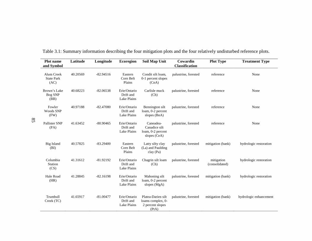
Table 3.1: Summary information describing the four mitigation plots and the four relatively undisturbed reference plots.
Plot name and Symbol
Latitude Longitude Ecoregion Soil Map Unit Cowardin Classification
Plot Type Treatment Type
Alum Creek State Park
(AC)
40.20569
-82.94516
Eastern
Corn Belt Plains
Condit silt loam,
0-1 percent slopes (CnA)
palustrine, forested
reference
None
Brown’s Lake Bog SNP
(BB)
40.68223 -82.06538 Erie/Ontario Drift and
Lake Plains
Carlisle muck (Ch)
palustrine, forested reference None
Fowler Woods SNP
(FW)
40.97188 -82.47080 Erie/Ontario Drift and
Lake Plains
Bennington silt loam, 0-2 percent
slopes (BnA)
palustrine, forested reference None
Pallister SNP (PA)
41.63452 -80.90465 Erie/Ontario Drift and
Lake Plains
Caneadea-Canadice silt
loam, 0-2 percent slopes (CeA)
palustrine, forested reference None
Big Island
(BI)
40.57825
-83.29400
Eastern
Corn Belt Plains
Latty silty clay
(La) and Paulding clay (Pa)
palustrine, forested
mitigation (bank)
hydrologic restoration
Columbia
Station (CS)
41.31612
-81.92192
Erie/Ontario
Drift and Lake Plains
Chagrin silt loam
(Ch)
palustrine, forested
mitigation
(consolidated)
hydrologic restoration
Hale Road
(HR)
41.28845
-82.16198
Erie/Ontario
Drift and Lake Plains
Mahoning silt
loam, 0-2 percent slopes (MgA)
palustrine, forested
mitigation (bank)
hydrologic restoration
Trumbull Creek (TC)
41.65917
-81.00477
Erie/Ontario Drift and
Lake Plains
Platea-Darien silt loams complex, 0-2 percent slopes
(PtA)
palustrine, forested
mitigation (bank)
hydrologic enhancement
85

Table 3.2: A description of the Vegetation Index of Biotic Integrity importance value metrics used for forested wetland evaluation (Mack 2009).
Metric Abbreviation Type Description Subcanopy IV
Importance value
The sum of the mean importance values for native shade-tolerant subcanopy species plus the mean importance value of facultative shade subcanopy species
Canopy IV Importance value The mean importance value of canopy species (species which at maturity will occupy the upper canopy of the forest even if at the time of sampling they are growing in the subcanopy
86
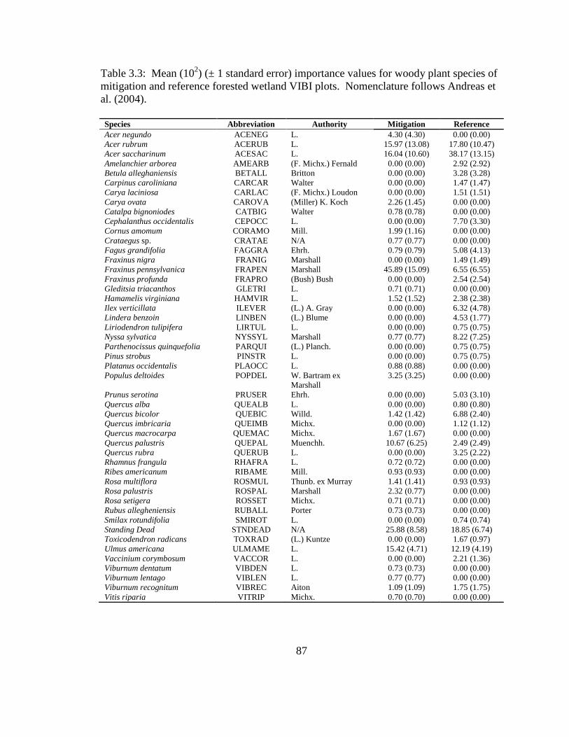
87
Table 3.3: Mean (102) (± 1 standard error) importance values for woody plant species of mitigation and reference forested wetland VIBI plots. Nomenclature follows Andreas et al. (2004). Species Abbreviation Authority Mitigation Reference Acer negundo ACENEG L. 4.30 (4.30) 0.00 (0.00) Acer rubrum ACERUB L. 15.97 (13.08) 17.80 (10.47) Acer saccharinum ACESAC L. 16.04 (10.60) 38.17 (13.15) Amelanchier arborea AMEARB (F. Michx.) Fernald 0.00 (0.00) 2.92 (2.92) Betula alleghaniensis BETALL Britton 0.00 (0.00) 3.28 (3.28) Carpinus caroliniana CARCAR Walter 0.00 (0.00) 1.47 (1.47) Carya laciniosa CARLAC (F. Michx.) Loudon 0.00 (0.00) 1.51 (1.51) Carya ovata CAROVA (Miller) K. Koch 2.26 (1.45) 0.00 (0.00) Catalpa bignoniodes CATBIG Walter 0.78 (0.78) 0.00 (0.00) Cephalanthus occidentalis CEPOCC L. 0.00 (0.00) 7.70 (3.30) Cornus amomum CORAMO Mill. 1.99 (1.16) 0.00 (0.00) Crataegus sp. CRATAE N/A 0.77 (0.77) 0.00 (0.00) Fagus grandifolia FAGGRA Ehrh. 0.79 (0.79) 5.08 (4.13) Fraxinus nigra FRANIG Marshall 0.00 (0.00) 1.49 (1.49) Fraxinus pennsylvanica FRAPEN Marshall 45.89 (15.09) 6.55 (6.55) Fraxinus profunda FRAPRO (Bush) Bush 0.00 (0.00) 2.54 (2.54) Gleditsia triacanthos GLETRI L. 0.71 (0.71) 0.00 (0.00) Hamamelis virginiana HAMVIR L. 1.52 (1.52) 2.38 (2.38) Ilex verticillata ILEVER (L.) A. Gray 0.00 (0.00) 6.32 (4.78) Lindera benzoin LINBEN (L.) Blume 0.00 (0.00) 4.53 (1.77) Liriodendron tulipifera LIRTUL L. 0.00 (0.00) 0.75 (0.75) Nyssa sylvatica NYSSYL Marshall 0.77 (0.77) 8.22 (7.25) Parthenocissus quinquefolia PARQUI (L.) Planch. 0.00 (0.00) 0.75 (0.75) Pinus strobus PINSTR L. 0.00 (0.00) 0.75 (0.75) Platanus occidentalis PLAOCC L. 0.88 (0.88) 0.00 (0.00) Populus deltoides POPDEL W. Bartram ex
Marshall 3.25 (3.25) 0.00 (0.00)
Prunus serotina PRUSER Ehrh. 0.00 (0.00) 5.03 (3.10) Quercus alba QUEALB L. 0.00 (0.00) 0.80 (0.80) Quercus bicolor QUEBIC Willd. 1.42 (1.42) 6.88 (2.40) Quercus imbricaria QUEIMB Michx. 0.00 (0.00) 1.12 (1.12) Quercus macrocarpa QUEMAC Michx. 1.67 (1.67) 0.00 (0.00) Quercus palustris QUEPAL Muenchh. 10.67 (6.25) 2.49 (2.49) Quercus rubra QUERUB L. 0.00 (0.00) 3.25 (2.22) Rhamnus frangula RHAFRA L. 0.72 (0.72) 0.00 (0.00) Ribes americanum RIBAME Mill. 0.93 (0.93) 0.00 (0.00) Rosa multiflora ROSMUL Thunb. ex Murray 1.41 (1.41) 0.93 (0.93) Rosa palustris ROSPAL Marshall 2.32 (0.77) 0.00 (0.00) Rosa setigera ROSSET Michx. 0.71 (0.71) 0.00 (0.00) Rubus allegheniensis RUBALL Porter 0.73 (0.73) 0.00 (0.00) Smilax rotundifolia SMIROT L. 0.00 (0.00) 0.74 (0.74) Standing Dead STNDEAD N/A 25.88 (8.58) 18.85 (6.74) Toxicodendron radicans TOXRAD (L.) Kuntze 0.00 (0.00) 1.67 (0.97) Ulmus americana ULMAME L. 15.42 (4.71) 12.19 (4.19) Vaccinium corymbosum VACCOR L. 0.00 (0.00) 2.21 (1.36) Viburnum dentatum VIBDEN L. 0.73 (0.73) 0.00 (0.00) Viburnum lentago VIBLEN L. 0.77 (0.77) 0.00 (0.00) Viburnum recognitum VIBREC Aiton 1.09 (1.09) 1.75 (1.75) Vitis riparia VITRIP Michx. 0.70 (0.70) 0.00 (0.00)

88
Table 3.4: Total number of live trees in each diameter class in mitigation and in reference plots. Plot abbreviations are provided in Table 3.1. Diameter Class (cm) Mitigation Plots Reference Plots BI CS HR TC AC BB FW PA 0 - < 1 41 4 49 1 0 0 0 8 1 - < 2.5 60 16 256 1 1 0 5 20 2.5 - < 5 87 38 300 1 9 4 14 30 5 - < 10 114 29 181 3 12 3 13 16 10 - < 15 83 17 34 4 13 6 11 2 15 - < 20 30 5 1 11 9 5 4 2 20 - < 25 0 14 0 6 4 5 0 1 25 - < 30 1 6 0 12 8 3 3 5 30 - < 35 0 5 0 10 3 8 5 1 35 - < 40 0 4 0 2 3 4 4 4 > 40 0 5 0 0 6 3 15 7

89
Table 3.5: Mean values (± 1 standard error) of soil characteristics from mitigation and reference forested wetlands. An asterisk indicates a significant difference in the mean values between mitigation and reference plots (Mann-Whitney test; p < 0.05).
Soil Characteristic Mitigation Reference soil reaction (pH) 5.89 (0.41) 5.23 (0.13) total phosphorus (μg/g) 8.60 (0.93) 44.98 (29.96)* total potassium (μg/g) 165.76 (25.87) 179.62 (15.92) total calcium (μg/g) 2031.66 (462.50) 3793.69 (811.67) total magnesium (μg/g) 396.73 (68.47) 619.18 (82.09) cation exchange capacity 21.24 (2.36) 41.78 (6.58)* % calcium 51.08 (13.27) 44.00 (4.08) % magnesium 16.30 (0.39) 12.67 (1.41) % potassium 2.04 (0.27) 1.20 (0.25) % nitrogen 0.25 (0.04) 0.84 (0.45) % carbon 2.40 (0.61) 10.47 (6.31) % organic matter 4.85 (0.10) 23.85 (13.46)
Table 3.6: Mean values (± 1 standard error) of physical attributes from mitigation and reference forested wetland plots. An asterisk indicates a significant difference in the mean values between mitigation and reference plots (Welch two-sample t-test; * p < 0.05).
Attribute Mitigation Reference depth of standing water 0.31 (0.31) 0.00 (0.00) litter depth 0.57 (0.26) 1.25 (0.43) number of tussocks 0.44 (0.36) 1.13 (0.24) number of hummocks 0.81 (0.81) 3.69 (1.08) number of macrotopographic depressions 2.25 (0.53) 3.75 (0.40) coarse woody debris 12-40 cm diameter 0.19 (0.19) 4.81 (1.36)* coarse woody debris >40 cm diameter 0.00 (0.00) 0.75 (0.45)

90
REFERENCES
Ahn, C., P.M. Gillevet, M. Sikaroodi and K.L. Wolf. 2009. An assessment of soil bacterial community structure and physicochemistry in two microtopographic locations of a palustrine forested wetland. Wetlands Ecology and Management 17:397-407.
Allen, J. A., B. D. Keeland, J. A. Stanturf, A. F. Clewell and H. E. Kennedy Jr. 2001. A Guide to Bottomland Hardwood Restoration: US Geological Survey, Biological Resources Division Information and Technology Report USGS/BRD/ITR-2000-0011, U.S. Department of Agriculture, Forest Service, Southern Research Station, General Technical Report SRS-40.
Alsfeld, A.J., J.L. Bowman and A. Deller-Jacobs. 2009. Effects of woody debris, microtopography, and organic matter amendments on the biotic community of constructed depressional wetlands. Biological Conservation 142:247-255.
Anderson, J.T., A.A. Landi and P.L. Marks. 2009. Limited flooding tolerance of juveniles restricts the distribution of adults in an understory shrub (Itea Virginica; Iteaceae). American Journal of Botany 96:1603-1611.
Andreas, B. K. 1989. The Vascular Flora of the Glaciated Allegheny Plateau Region of Ohio. Bulletin of the Ohio Biological Survey, Volume 8, Number 1. The Ohio State University, Columbus, Ohio.
Andreas, B. K., J. J. Mack and J. S. McCormac. 2004. Floristic quality assessment index (FQAI) for vascular plants and mosses for the state of Ohio. Ohio Environmental Protection Agency, Division of Surface Water, Wetland Ecology Group, Columbus, Ohio.
Baldwin, R.F., A.J.K. Calhoun and P.G. deMaynadier. 2006. Conservation planning for amphibian species with complex habitat requirements: A case study using movements and habitat selection of the Wood Frog (Rana sylvatica). Journal of Herpetology 40:442-453.

91
Batzer, D.P., S.E. Dietz-Brantley, B.E. Taylor and A.E. DeBiase. 2005. Evaluating regional differences in macroinvertebrate communities from forested depressional wetlands across eastern and central North America. Journal of the North American Benthological Society 24:403-414.
Benson, T.J. and J.C. Bednarz. 2010. Short-term effects of flooding on understory habitat and presence of Swainson's warblers. Wetlands 30:29-37.
Blood, L.E. and J.H. Titus. 2010. Microsite effects on forest regeneration in a bottomland swamp in western New York. Journal of the Torrey Botanical Society 137:88-102.
Braccia, A. and D.P. Batzer. 2001. Invertebrates associated with woody debris in a southeastern US forested floodplain wetland. Wetlands 21:18-31.
Braun, E. L. 1961. The Woody Plants of Ohio. Ohio State University Press, Columbus, Ohio.
Braun, E. L. 1950. Deciduous Forests of Eastern North America. Hafner Publishing Company Inc., New York, New York.
Brinson, M.M. and R. Rheinhardt. 1996. The role of reference wetlands in functional assessment and mitigation. Ecological Applications 6:69-76.
Cowardin, L. M., V. Carter, F. C. Golet and E. T. LaRoe. 1979. Classification of wetlands and deepwater habitats of the United States. Department of the Interior, Fish and Wildlife Service, Washington D.C.
D'Amato, A.W., D.A. Orwig and D.R. Foster. 2009. Understory vegetation in old-growth and second-growth Tsuga canadensis forests in western Massachusetts. Forest Ecology and Management 257:1043-1052.
Eriksson, O. and H. Froborg. 1996. ''Windows of opportunity'' for recruitment in long-lived clonal plants: Experimental studies of seedling establishment in Vaccinium shrubs. Canadian Journal of Botany 74:1369-1374.
Ervin, G.N., L.C. Majure and J.T. Bried. 2006. Influence of long-term greentree reservoir impoundment on stand structure, species composition, and hydrophytic indicators. Journal of the Torrey Botanical Society 133:468-481.
Gordon, R. B. 1969. Natural Vegetation of Ohio in Pioneer Days. Bulletin of the Ohio Biological Survey, Volume 3, Number 2. The Ohio State University, Columbus, Ohio.

92
Hoover, J.P. 2009. Effects of hydrologic restoration on birds breeding in forested wetlands. Wetlands 29:563-573.
Huenneke, L.F. and R.R. Sharitz. 1986. Microsite abundance and distribution of woody seedlings in a South-Carolina cypress-tupelo swamp. American Midland Naturalist 115:328-335.
Jordan, R.A. and J.M. Hartman. 1995. Safe sites and the regeneration of Clethra alnifolia L (Clethraceae) in wetland forests of central New-Jersey. American Midland Naturalist 133:112-123.
Kaminski, R.M., R.W. Alexander and B.D. Leopold. 1993. Wood duck and mallard winter microhabitats in Mississippi hardwood bottomlands. Journal of Wildlife Management 57:562-570.
Kanno, H. and K. Seiwa. 2004. Sexual vs. vegetative reproduction in relation to forest dynamics in the understory shrub, Hydrangea paniculata (Saxifragaceae). Plant Ecology 170:43-53.
Karraker, N.E. and J.P. Gibbs. 2009. Amphibian production in forested landscapes in relation to wetland hydroperiod: A case study of vernal pools and beaver ponds. Biological Conservation 142:2293-2302.
Kettlewell, C.I., V. Bouchard, D. Porej, M. Micacchion, J.J. Mack, D. White and L. Fay. 2008. An assessment of wetland impacts and compensatory mitigation in the Cuyahoga River Watershed, Ohio, USA. Wetlands 28:57-67.
King, S.L., J.A. Allen and J.W. McCoy. 1998. Long-term effects of a lock and dam and greentree reservoir management on a bottomland hardwood forest. Forest Ecology and Management 112:213-226.
Kozlowski, T.T. 1984. Plant responses to flooding of soil. Bioscience 34:162-167.
Kruse, B.S. and J.W. Groninger. 2003. Vegetative characteristics of recently reforested bottomlands in the lower Cache River Watershed, Illinois, USA. Restoration Ecology 11:273-280.
Laidig, K.J., R.A. Zampella and C. Popolizio. 2009. Hydrologic regimes associated with Helonias bullata L. (swamp pink) and the potential impact of simulated water-level reductions. Journal of the Torrey Botanical Society 136:221-232.
Larson, A.J. and J.F. Franklin. 2010. The tree mortality regime in temperate old-growth coniferous forests: the role of physical damage. Canadian Journal of Forest Research 40:2091-2103.

93
Lindenmayer, D. B. and J. F. Franklin. 2002. Conserving Forest Biodiversity: A Comprehensive Multiscaled Approach. Island Press, Washington D.C.
Mack, J. J. and M. Micacchion. 2006. An ecological assessment of Ohio mitigation banks: vegetation, amphibians, hydrology, and soils. Ohio EPA Technical Report WET/2007-2. Ohio Environmental Protection Agency, Division of Surface, Wetland Ecology Group, Columbus, Ohio.
Mack, J. J. 2007a. Automated spreadsheets for calculating and reporting the Vegetation Index of Biotic Integrity (VIBI) metrics and scores v. 1.0.1. Ohio EPA Technical Report WET/2006-1. Ohio Environmental Protection Agency, Wetland Ecology Group, Division of Surface Water, Columbus, Ohio.
Mack, J. J. 2007b. Integrated wetland assessment program, part 9: field manual for the Vegetation Index of Biotic Integrity for Wetlands v. 1.4. Ohio EPA Technical Report WET/2007-6. Ohio Environmental Protection Agency, Wetland Ecology Group, Division of Surface Water, Columbus, Ohio.
Mack, J.J. 2009. Development issues in extending plant-based IBIs to forested wetlands in the Midwestern United States. Wetlands Ecology and Management. 17:117-130.
Matlaga, D.P. and C.C. Horvitz. 2009. Growth and survival across a gap-understory gradient: contrast in performance of sexually vs. clonally produced offspring. American Journal of Botany 96:439-447.
McCune, B. and J. B. Grace . 2002. Analysis of Ecological Communities. MJM Software, Gleneden Beach, Oregon.
McCune, B. and M.J. Mefford. 2006. PC-ORD. Multivariate analysis of ecological data. Version 5. MjM Software, Glenedon Beach, Oregon.
Micacchion, M. and B.D. Gara. 2008. An ecological and functional assessment of urban wetlands in central Ohio, volume 3: comparisons of the amphibian communities of urban and reference wetlands using level 1, 2 and 3 assessment tools. Ohio EPA Technical Report WET/2008-1. Ohio Environmental Protection Agency, Wetland Ecology Group, Division of Surface Water, Columbus, Ohio.
Micacchion, M., B. D. Gara and J. J. Mack. 2010. Assessment of wetland mitigation projects in Ohio,volume 1: an ecological assessment of Ohio individual wetland mitigation projects. Ohio EPA Technical Report WET/2010-1A. Ohio Environmental Protection Agency, Wetland Ecology Group, Division of Surface Water, Columbus, Ohio.
94
Mielke Paul W., J. and K. J. Berry . 2001. Permutation Methods: A Distance Function Approach. Springer Series in Statistics, New York, New York.
Mitsch, W. J. and J. G. Gosselink. 2007. Wetlands, 4th edition. John Wiley and Sons, New York.
Moser, K.F., C. Ahn and G.B. Noe. 2009. The influence of microtopography on soil nutrients in created mitigation wetlands. Restoration Ecology 17:641-651.
National Research Council. 2001. Compensating for Wetland Losses Under the Clean Water Act. National Academy Press, Washington D.C.
Neatrour, M.A., R.H. Jones and S.W. Golladay. 2005. Correlations between soil nutrient availability and fine-root biomass at two spatial scales in forested wetlands with contrasting hydrological regimes. Canadian Journal of Forest Research 35:2934-2941.
Neatrour, M.A., R.H. Jones and S.W. Golladay. 2007. Response of three floodplain tree species to spatial heterogeneity in soil oxygen and nutrients. Journal of Ecology 95:1274-1283.
Oksanen, J., F. G. Blanchet, R. Kindt, P. Legendre, R. G. Ohara, G. L. Simpson, M. H. H. Stevens and H. Wagner 2010. vegan: Community ecology package. R package version 1.17-0. Available online at: http://CRAN.R-project.org/package=vegan. Accessed April 16, 2011.
Oliver, C.D. and Larson, B.C. 1996. Forest Stand Dynamics, Update Edition. John Wiley and Sons, Inc., New York.
Peet, R.K. and N.L. Christensen. 1987. Competition and tree death. Bioscience 37:586-595.
Peet, R.K., T.R. Wentworth and P.S. White. 1998. A flexible, multipurpose method for recording vegetation composition and structure. Castanea 63: 262-274.
Porej, D. 2003. Faunal aspects of wetland restoration. Ph.D. Dissertation. The Ohio State University, Columbus, Ohio.
Porej, D., M. Micacchion and T.E. Hetherington. 2004. Core terrestrial habitat for conservation of local populations of salamanders and wood frogs in agricultural landscapes. Biological Conservation 120:399-409.

95
R Development Core Team. 2009. R: a language and environment for statistical computing. R Foundation for Statistical Computing, Vienna, Austria. ISBN 3-900051-07-0. Available online AT: http://www.R-project.org. Accessed April 16, 2011.
Reed, P. B. J. 1988. National list of plant species that occur in wetlands: national summary. Department of the Interior, Fish and Wildlife Service, Washington D.C.
Riffell, S., T. Burton and M. Murphy. 2006. Birds in depressional forested wetlands: area and habitat requirements and model uncertainty. Wetlands 26:107-118.
Ruzicka, K.J., J.W. Groninger and J.J. Zaczek. 2010. Deer browsing, forest edge effects, and vegetation dynamics following bottomland forest restoration. Restoration Ecology 18:702-710.
Scanga, S.E. and D.J. Leopold. 2010. Population vigor of a rare, wetland, understory herb in relation to light and hydrology. Journal of the Torrey Botanical Society 137:297-311.
Schoenholtz, S.H., J.P. James, R.M. Kaminski, B.D. Leopold and A.W. Ezell. 2001. Afforestation of bottomland hardwoods in the Lower Mississippi Alluvial Valley: status and trends. Wetlands 21:602-613.
Soil Survey Staff, Natural Resources Conservation Service, United States Department of Agriculture. Soil survey geographic (SSURGO) database for Ashtabula, Delaware, Lorain, Marion, Richland and Wayne Counties, Ohio. Available online at http://soildatamart.nrcs.usda.gov. Accessed April 16, 2011.
The Nature Conservancy. 2011. Brown's Lake Bog Preserve. Available online at http://www.nature.org/ourinitiatives/regions/northamerica/unitedstates/ohio/placesweprotect/browns-lake-bog-preserve.xml. Accessed April 16, 2011.
The Ohio Agricultural Research and Development Center, Service Testing and Research Laboratory (STAR Lab). 2011. Methods and References. Available online at: http://oardc.osu.edu/starlab/references.asp. Accessed April 16, 2011.
Titus, H.J. 1990. Microtopography and woody plant regeneration in a hardwood floodplain swamp in Florida. Bulletin of the Torrey Botanical Club 117:429-437.
Van Pelt, R. and J.F. Franklin. 2000. Influence of canopy structure on the understory environment in tall, old-growth, conifer forests. Canadian Journal of Forest Research 30:1231-1245.

96
Vivian-Smith, G. 1997. Microtopographic heterogeneity and floristic diversity in experimental wetland communities. Journal of Ecology 85: 71-82.
Woods, A. J., J. M. Omernik, C. S. Brockman, T. D. Gerber, W. D. Hosteter and S. H. Azevedo 1998. Ecoregions of Indiana and Ohio, 1:1500000. Available at http://www.epa.gov/wed/pages/ecoregions/ohin_eco.htm. Accessed May 28, 2011.

97
CHAPTER 4
USING THE VEGETATION INDEX OF BIOTIC INTEGRITY TO COMPARE
FORESTED MITIGATION WETLANDS AND RELATIVELY UNDISTURBED
REFERENCE FORESTED WETLANDS
Abstract
The Vegetation Index of Biotic Integrity (VIBI) is currently used by regulatory
agencies in Ohio to assess wetland quality. It uses several plant community metrics,
tailored to specific wetland types, to quantitatively characterize wetland plant
communities for regulatory purposes. We utilized the VIBI for forested wetlands (VIBI-
Forest) to compare the plant communities of four mitigation forested wetlands with four
relatively undisturbed reference forested wetlands within the Erie/Ontario Drift and Lake
Plains and Eastern Corn Belt Plains ecoregions of Ohio. Mean values for VIBI-Forest
score (p = 0.01), Floristic Quality Assessment Index (FQAI) score (p = 0.03), percent
cover of sensitive species (p = 0.03), and importance values of subcanopy species (p =
0.03) were all significantly higher for reference plots compared to values calculated for
mitigation plots. NMDS ordinations indicated that reference plots were positively
associated with metrics related to FQAI score, number of seedless vascular plants,
number of plants that tolerate at least partial shade, importance of woody subcanopy

98
species, and percent cover of bryophytes, hydrophytes and sensitive plant species. The
ordinations also indicated an association between mitigation plots and metrics that reflect
the importance of woody canopy species, percent cover of plants with a wide range of
ecological tolerances and density of small trees. All four reference wetlands were
classified as Superior Quality Wetland Habitat based on Wetland Tiered Aquatic Life
Use categories. Three mitigation plots produced scores in the range of Restorable
Wetland Habitat and one qualified as Limited Quality Wetland Habitat. Our results were
consistent with those from other studies that used the VIBI for forested wetland
evaluation, and they provide additional support for the use of the VIBI-Forest for forested
wetland assessments in Ohio.
Introduction
Quantitative biological assessment methods have become important for regulatory
agencies responsible for characterizing ecosystems. Many of the methods currently in
use can be classified as indices of biotic integrity (IBIs) which use several metrics that,
when combined, characterize overall biotic integrity (Karr 1991). Some of the earliest
applications of IBIs focused on the assessment of fish and macroinvertebrate
communities (Karr 1981, Fausch et al. 1984, Kerans and Karr 1994). More recently, IBIs
were developed for use with other taxa including birds (O’Connell et al. 2000, DeLuca et
al. 2004), periphyton (Hill et al. 2000) and zooplankton (Lougheed and Chow-Fraser
2002). However, few IBIs have been developed that consider plant community
characteristics.

99
Beginning in 1996, ecologists at the Ohio Environmental Protection Agency
focused on developing biological assessment methods for wetlands. The goal was to
develop quantitative techniques that could be used by the regulatory community to assess
the biological integrity of wetlands. The Vegetation Index of Biotic Integrity for
Wetlands (VIBI) was first presented in the literature in 2000 (Mack et al. 2000), and
since that time it has been regularly used to assess wetland condition in Ohio (Mack and
Micacchion 2006, Micacchion and Gara 2008, Micacchion et al. 2010). Since the initial
protocol was published, additional testing iterations with larger datasets have resulted in
refined VIBI metrics and expanded applications to specific wetland types (Mack 2001,
Mack et al. 2008, Mack 2009). Furthermore, Wetland Tiered Aquatic Life Use
categories were developed that allow VIBI scores to be translated into specific designated
uses for wetlands (Mack 2004).
Applying the VIBI to forested wetlands in Ohio was particularly challenging
because: (1) forest canopies may remain intact even after the herb and shrub strata are
significantly disturbed, and (2) increases in diversity may be undesirable in forested
wetlands if the increase is due to the establishment of shade-intolerant species following
disturbance (Mack 2009). However, continued evaluation and revision of the plant
community metrics used in the VIBI for forested wetlands (VIBI-Forest) resulted in a set
of ten metrics that characterize forested wetland condition. Additionally, the modified set
of VIBI-Forest metrics corrected problems that plagued previous versions, most notably
the sensitivity of metrics to increases in diversity following disturbance (Mack 2004,
2009).

100
The VIBI is currently used by both federal and state regulatory agencies to
evaluate the condition of wetlands in Ohio. The most consistent use has been for the
assessment of wetland mitigation bank performance. The Interagency Review Team,
which consists of representatives from the U.S. Army Corps of Engineers, U.S. Fish and
Wildlife Service, U.S. Environmental Protection Agency, Ohio Department of Natural
Resources, Natural Resources Conservation Service and the Ohio Environmental
Protection Agency, uses VIBI data to assess the plant community characteristics of
mitigation banks and determine appropriate credit release schedules (U.S. Army Corps of
Engineers, personal communication 2011). Given the importance of the VIBI for
wetland assessment in Ohio, we used the VIBI-Forest to characterize both forested
mitigation wetlands and relatively undisturbed reference forested wetlands in Ohio. The
objective of this chapter is to characterize and compare mitigation and reference forested
wetlands using results from the VIBI-Forest.
Study Area and Methods
Chapters 2 and 3 of this thesis provide detailed descriptions of the four mitigation
study areas and the four relatively undisturbed reference study areas (Figure 4.1). Table
4.1 summarizes the characteristics of the eight study area locations. Detailed descriptions
of the methods used to collect herbaceous vegetation data (Chapter 2), woody vegetation
data (Chapter 3) and soil and physical attribute data (Chapters 2 and 3) are provided in
earlier chapters. A complete description of the VIBI data collection protocol which was
followed for this study is provided in the VIBI field manual (Mack 2007b).

101
Vegetation Data Reduction and Metric Calculations
To calculate a VIBI-Forest score for each plot, a series of data reductions and
metric calculations were necessary as outlined in the VIBI field manual (Mack 2007b).
Data reduction calculations were completed using the Microsoft Excel spreadsheet
created by Mack (2007a) specifically for VIBI data analysis. Detailed descriptions of the
metrics used to produce VIBI-Forest scores are included in Table 4.2.
Statistical Analyses
Differences in the mean values of overall VIBI-Forest scores and individual
metric values were determined using Welch’s two-sample t-tests and Mann-Whitney
nonparametric tests for group differences. Prior to testing for significant group
differences, a Shapiro-Wilk test for normality was used to determine whether a
parametric or nonparametric procedure was most appropriate for each analysis. A
significance level of 0.05 was used to evaluate if differences between groups were
statistically significant.
Nonmetric multidimensional scaling analysis (NMDS) was used to examine
herbaceous and woody plant community composition in relation to the VIBI-Forest
metric scores (Figure 4.2). NMDS is generally the most effective ordination method to
use on ecological data sets and its advantages include: (1) avoiding assumptions of linear
relationships among variables, (2) relieving the “zero truncation problem” associated
with all ordinations of community data sets, and (3) allowing the use of any distance
measure or relativation (McCune and Grace 2002). NMDS uses an iterative search to

102
converge on a solution that minimizes “stress” in the configuration. Stress is a function
of a linear monotone transformation of observed dissimilarities and ordination distances.
The NMDS procedure was performed using the VEGAN metaMDS function (Oksanen et
al. 2010) in the R statistical computing program (R Development Core Team 2009). The
relationship between plant community composition and the VIBI-Forest metric values
was examined by fitting vectors representing the ten VIBI-Forest metrics to the
ordinations (Figure 4.2).
Results
VIBI Metrics
The results of the tests of group differences indicated that there are significant
differences between mitigation and reference plots in overall VIBI-Forest score (p =
0.01), FQAI score (p = 0.03), percent cover of sensitive plant species (p = 0.03), and the
importance of woody subcanopy species (p = 0.03) (Figure 4.3, Table 4.3).
Nonmetric Multidimensional Scaling
The NMDS analysis of herbaceous plant species relative cover values converged
on a stable solution after five tries with a final stress value of 5.98. The NMDS analysis
of woody plant species importance values converged on a stable solution after one try
with a final stress value of 3.53. The ordination plots depict sample plot positions
relative to vectors representing VIBI-Forest metric values (Figure 4.2). The vectors point
in the direction of the most rapid change in the metric value scores. The ordination of

103
herbaceous plant species relative covers (Figure 4.2a) and the ordination of woody plant
species importance values (Figure 4.2b) showed similar trends. In both ordinations,
reference plots were generally associated with metrics related to the occurrence of shade-
tolerant species (shade), FQAI score (FQAI), importance of subcanopy species
(subcanopy IV), relative cover of seedless vascular plants (SVP), and percent cover
values for bryophytes (% bryophyte), hydrophytes (% hydrophyte) and sensitive species
(% sensitive). Mitigation plots were generally associated with metrics related to the stem
density of small trees (small tree), percent cover of species with a wide range of
ecological tolerances (% tolerant) and the importance of canopy tree species (canopy IV)
(Figure 4.2). A detailed description of the metrics is provided in Table 4.2.
Discussion
VIBI Scores
Our results indicate that the metrics developed for these study areas using VIBI-
Forest are accurate indicators of forested wetland biological integrity. The significantly
higher mean VIBI-Forest score for reference wetlands (Figure 4.3) compared with the
score for mitigation wetlands agrees with the results from other studies that used the VIBI
to compare natural and mitigation wetlands in Ohio (Mack and Micacchion 2006,
Micacchion and Gara 2008, Micacchion et al. 2010,). Additionally, the significantly
higher values of FQAI, SVP and % sensitive metrics for reference plots suggests that
reference plots may provide habitat that favors the establishment of seedless vascular
plants (i.e., ferns and fern allies) and plants thought to have a narrow range of ecological

104
tolerances (Andreas et al. 2004). Though not statistically significant, mean values for
shade, % bryophyte and % hydrophyte metrics were higher for reference plots. This
trend suggests that conditions in reference forested wetlands may be more favorable to
the establishment and persistence of shade-tolerant plants, mosses and some liverworts,
and plants adapted to wet environments than conditions in mitigation plots.
Mitigation plots had higher mean values for the % tolerant, small tree and canopy
IV metrics. These higher values indicate a tendency for mitigation forested wetlands to
support more species believed to have a wide range of ecological tolerances (Andreas et
al. 2004) and more trees in smaller diameter classes. The higher mean canopy IV metric
value indicates that tree species that would be dominant canopy species at maturity are
more important in mitigation plots than in reference plots. As we discussed in Chapters 2
and 3, two of the mitigation plots, Hale Road (HR) and Big Island (BI) are young forests
in the stem exclusion stage of forest development. This stage is characterized by many
young trees competing for position in the canopy (Peet and Christensen 1987, Oliver and
Larson 1996). The canopies of these two plots are dominated by Fraxinus
pennsylvanica. The dominance of this species and the corresponding high canopy IV
metric value that characterizes young, disturbed forested wetlands has been noted by
Mack (2004, 2009).
In Chapters 2 and 3, we discussed how physical attributes, physiographic factors
and landscape position may have influenced plant community composition and structure
of the sample plots. Given that the VIBI-Forest metric values are directly influenced by
plant community composition and structure, the same plot characteristics we discussed in

105
the earlier chapters (e.g., forest development stage and physical habitat attributes) likely
influenced the VIBI-Forest metric scores. The significantly higher number of seedless
vascular plants in reference plots can be attributed to the availability of suitable
microsites (e.g., coarse woody debris and hummocks) that are important for fern
colonization in forests and can be lacking in areas recovering from agricultural land use
(Flinn 2007). In addition, the presence of physical attributes that provide elevated
microsites may help explain the significantly higher subcanopy IV metric values of
reference plots. Other authors have documented the influence of microsites on woody
plant establishment in forested wetlands (Huenneke and Sharitz 1986, Titus 1990, Blood
and Titus 2010), and this topic is discussed in detail in Chapter 3 of this thesis.
The NMDS ordinations of herbaceous plant species relative covers and woody
plant species importance values (Figure 4.3) show the relationship between the species
compositions of sample plots and the VIBI-Forest metric scores. Several of the metrics
(shade, FQAI, % hydrophyte, % sensitive and % tolerant) are influenced by both
herbaceous and woody plant species while others like small tree, subcanopy IV and
canopy IV capture important aspects of woody plant community structure. Both
ordinations generally illustrate the same trend: reference plots were associated with
higher shade, SVP, % bryophyte, % hydrophyte, % sensitive and subcanopy IV metric
values, and mitigation plots were associated with small tree, % tolerant and canopy IV
metric values (Figure 4.2). These ordinations support results reported by Mack (2009)
who showed that high quality forested wetlands were associated with shade, FQAI, %
106
hydrophyte, % sensitive, SVP metrics and subcanopy IV metrics and that low quality
wetlands were associated with small tree, % tolerant and canopy IV metrics.
Wetland Tiered Aquatic Life Use Designations
One goal that drove the development of quantitative wetland assessment methods
for Ohio wetlands was the desire to relate biological integrity to specific uses for
wetlands (Mack 2001, 2004). In response, Mack (2004) published Tiered Aquatic Life
Use (TALU) categories for Ohio wetlands. The wetland TALU categories were proposed
using plant community, landscape position and ecoregional considerations (Mack 2004).
The general categories are: Superior Wetland Habitat (SWLH), Wetland Habitat (WLH),
Restorable Wetland Habitat (RWLH) and Limited Quality Wetland Habitat (LQWLH)
(Table 4.4). These categories correspond to wetland antidegradation categories (i.e.,
Category 1, 2 or 3) as specified by Ohio Administrative Code 3745-1-54 (Mack 2004).
Table 4.5 provides depressional forested wetland VIBI scoring breaks for the TALU
categories. Scoring breaks for all other wetland types are provided by Mack (2004, Table
11). It is important to note that wetlands within the Erie/Ontario Drift ad Lake Plains
(EOLP) ecoregion are held to higher scoring standards than wetlands within all other
ecoregions. This is due to the significantly higher VIBI scores found for EOLP wetlands
when compared with wetlands from other ecoregions (Mack 2004). All four reference
forested wetland plots in this study produced overall VIBI-Forest scores within the
scoring range of SWLH. One mitigation plot (BI) produced a VIBI-Forest score in the
range of LQWLH while the other three were categorized as RWLH (Table 4.6). The

107
very low score for BI (9) was likely driven by the dominance of the invasive, non-native
plant Lysimachia nummularia in the herbaceous layer. Our results are consistent with
those from a study of Ohio wetland mitigation banks in which more than 90% of the
wetland areas evaluated were categorized as either LQWLH or RWLH and none of the
sampled mitigation wetlands produced scores in the range of SWLH (Mack and
Micacchion 2006).
Conclusions
Our results provide support for the use of the VIBI-Forest in assessing biological
integrity of forested wetlands in Ohio. The ten metrics presented by Mack (2009)
characterize plant community attributes associated with forest understories as well as
forest canopies and appeared to separate relatively undisturbed forested wetlands from
those that have been disturbed or manipulated by humans. To reiterate our conclusions
from the previous chapters, the techniques used to restore, establish and (or) enhance
forested wetlands for use as wetland mitigation generally result in plant communities in a
range of development stages that have inherently different compositions and structures.
As the plant communities of forested mitigation wetlands continue to develop and new
mitigation projects are completed, there will be increased opportunity to study plant
community development in these areas. Nevertheless, the results presented in this
chapter provide support for the VIBI-Forest as a way of assessing the plant communities
of forested wetlands in Ohio and represents a point from which additional research can be
conducted.

108
Figure 4.1: Locations of the four forested wetland mitigation plots (black dots) and the four relatively undisturbed reference forested wetland plots (open circles).

109
(a)
(b)
Figure 4.2: Nonmetric multidimensional scaling ordinations of mitigation and reference forested wetland plots based on (a) herbaceous species relative cover values and (b) woody plant species importance values. Vectors represent VIBI-Forest metric values. A complete description of the VIBI-Forest metrics is provided in Table 4.2.
NMDS 1
-0.8 -0.6 -0.4 -0.2 0.0 0.2 0.4 0.6 0.8
NM
DS
2
-1.0
-0.8
-0.6
-0.4
-0.2
0.0
0.2
0.4
0.6
0.8
mitigation reference
TC
PA
HR
BI
CS
FW
AC
BB
can IV
% tolsmall tree
% bry% sen
SVP
sub IVFQAI % hydshade
NMDS 1
-0.8 -0.6 -0.4 -0.2 0.0 0.2 0.4 0.6 0.8 1.0 1.2
NM
DS
2
-1.0
-0.8
-0.6
-0.4
-0.2
0.0
0.2
0.4
0.6
0.8
mitigation reference
TC
PA
HR
BI
CS
AC
FW BB
can IV
% tol
small tree
shade
% bry
% hydr% sen
sub IV
FQAI
SVP

110
Figure 4.3: Mean (± 1 standard error) VIBI-Forest scores for mitigation and reference forested wetland plots. Means of the two plot types were significantly different (p = 0.01).
mitigation reference
Mea
n VI
BI-F
ores
t Sco
re
0
20
40
60
80
100

Table 4.1: Summary information describing the four mitigation plots and the four relatively undisturbed reference plots.
Plot name and Symbol
Latitude Longitude Ecoregion Soil Map Unit Cowardin Classification
Plot Type Treatment Type
Alum Creek State Park
(AC)
40.20569
-82.94516
Eastern Corn Belt
Plains
Condit silt loam, 0-1
percent slopes (CnA)
palustrine, forested
reference
None
Brown’s Lake Bog SNP
(BB)
40.68223 -82.06538 Erie/Ontario Drift and Lake Plains
Carlisle muck (Ch) palustrine, forested reference None
Fowler Woods SNP
(FW)
40.97188 -82.47080 Erie/Ontario Drift and Lake Plains
Bennington silt loam, 0-2 percent
slopes (BnA)
palustrine, forested reference None
Pallister SNP
(PA)
41.63452
-80.90465
Erie/Ontario Drift and Lake Plains
Caneadea-Canadice
silt loam, 0-2 percent slopes
(CeA)
palustrine, forested
reference
None
Big Island
(BI)
40.57825
-83.29400
Eastern Corn Belt
Plains
Latty silty clay (La) and Paulding clay
(Pa)
palustrine, forested
mitigation (bank)
hydrologic restoration
Columbia
Station (CS)
41.31612
-81.92192
Erie/Ontario Drift and Lake Plains
Chagrin silt loam
(Ch)
palustrine, forested
mitigation
(consolidated)
hydrologic restoration
Hale Road
(HR)
41.28845
-82.16198
Erie/Ontario Drift and Lake Plains
Mahoning silt loam, 0-2 percent slopes
(MgA)
palustrine, forested
mitigation (bank)
hydrologic restoration
Trumbull Creek (TC)
41.65917
-81.00477
Erie/Ontario Drift and Lake Plains
Platea-Darien silt loams complex, 0-2 percent slopes (PtA)
palustrine, forested
mitigation (bank)
hydrologic enhancement
111
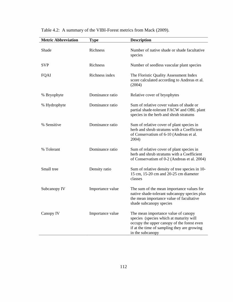
112
Table 4.2: A summary of the VIBI-Forest metrics from Mack (2009).
Metric Abbreviation Type Description Shade
Richness
Number of native shade or shade facultative species
SVP Richness Number of seedless vascular plant species
FQAI Richness index The Floristic Quality Assessment Index score calculated according to Andreas et al. (2004)
% Bryophyte Dominance ratio Relative cover of bryophytes
% Hydrophyte Dominance ratio Sum of relative cover values of shade or partial shade-tolerant FACW and OBL plant species in the herb and shrub stratums
% Sensitive Dominance ratio Sum of relative cover of plant species in herb and shrub stratums with a Coefficient of Conservatism of 6-10 (Andreas et al. 2004)
% Tolerant Dominance ratio Sum of relative cover of plant species in herb and shrub stratums with a Coefficient of Conservatism of 0-2 (Andreas et al. 2004)
Small tree Density ratio Sum of relative density of tree species in 10-15 cm, 15-20 cm and 20-25 cm diameter classes
Subcanopy IV Importance value The sum of the mean importance values for native shade-tolerant subcanopy species plus the mean importance value of facultative shade subcanopy species
Canopy IV Importance value The mean importance value of canopy species (species which at maturity will occupy the upper canopy of the forest even if at the time of sampling they are growing in the subcanopy

Table 4.3: A summary of the VIBI-Forest metric values for mitigation and reference plots. An asterisk indicates a significant difference in the mean metric value between mitigation and reference plots (p < 0.05). A detailed description of the metrics is provided in Table 4.2 and study plot abbreviations are included in Table 4.1.
VIBI-Forest Metrics Mitigation Plots Reference Plots BI CS HR TC mean AC BB FW PA mean Shade 6.00 26.00 10.00 17.00 14.80 35.00 28.00 21.00 22.00 26.50 SVP 0.00 1.00 0.00 3.00 1.00 1.00 5.00 2.00 5.00 3.25 FQAI 17.10 23.00 15.10 22.10 19.33 25.10 25.30 24.20 31.60 26.55* % Bryophyte 0.02 0.00 0.01 0.07 0.03 0.08 0.03 0.20 0.05 0.09 % Hydrophyte 0.01 0.20 0.01 0.15 0.09 0.45 0.90 0.12 0.50 0.49 % Sensitive 0.01 0.02 0.30 0.04 0.09 0.38 0.64 0.60 0.83 0.61* % Tolerant 0.59 0.72 0.06 0.46 0.46 0.24 0.28 0.05 0.01 0.15 Small Tree 0.24 0.2 0.03 0.25 0.18 0.19 0.13 0.11 0.04 0.12 Subcanopy IV 0.00 0.04 0.00 0.06 0.03 0.07 0.17 0.08 0.14 0.12* Canopy IV 0.22 0.16 0.26 0.19 0.21 0.16 0.16 0.16 0.16 0.16
113

114
Table 4.4: Descriptions of the Wetland Tiered Aquatic Life Use categories (TALUs) from Mack (2004)
Designation Code Definition
Superior Wetland Habitat
SWLH Wetlands that are capable of supporting and maintaining a high quality community with species composition, diversity, and functional organization comparable to the vegetation IBI score of at least 83% (five-sixths) of the 95th percentile for the appropriate wetland type and region.
Wetland Habitat WLH Wetlands that are capable of supporting and maintaining a balanced, integrated, adaptive community having a species composition, diversity, and functional organization comparable to the vegetation IBI score of at least 66% (two-thirds) of the 95th percentile for the appropriate wetland type and region.
Restorable Wetland Habitat RWLH Wetlands which are degraded but have a reasonable potential for regaining the capability of supporting and maintaining a balanced, integrated, adaptive community of vascular plants having a species composition, diversity, and functional organization comparable to the vegetation IBI score of at least 33% (one-third) of the 95th percentile distribution for the appropriate wetland type and region.
Limited Quality Wetland Habitat
LQWLH Wetlands which are seriously degraded and which do not have a reasonable potential for regaining the capability of supporting and maintaining a balanced, integrated, adaptive community having a species composition, diversity, and functional organization comparable to the vegetation IBI score of less 33% (one-third) of the 95th percentile for the appropriate wetland type and region.
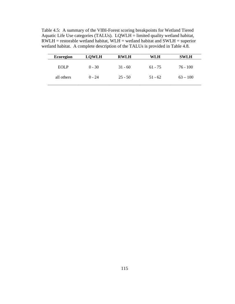
115
Table 4.5: A summary of the VIBI-Forest scoring breakpoints for Wetland Tiered Aquatic Life Use categories (TALUs). LQWLH = limited quality wetland habitat, RWLH = restorable wetland habitat, WLH = wetland habitat and SWLH = superior wetland habitat. A complete description of the TALUs is provided in Table 4.8.
Ecoregion LQWLH RWLH WLH SWLH
EOLP
0 - 30
31 - 60
61 - 75
76 - 100
all others 0 - 24 25 - 50 51 - 62 63 – 100
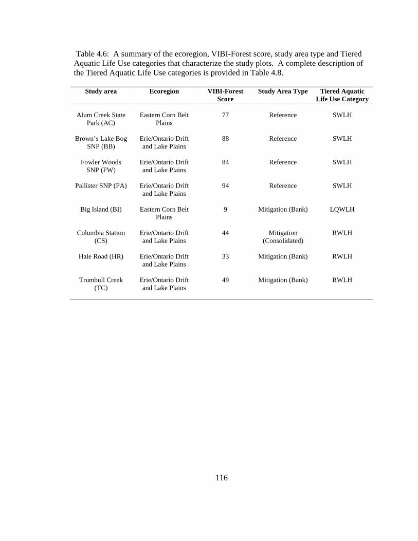
116
Table 4.6: A summary of the ecoregion, VIBI-Forest score, study area type and Tiered Aquatic Life Use categories that characterize the study plots. A complete description of the Tiered Aquatic Life Use categories is provided in Table 4.8.
Study area Ecoregion VIBI-Forest Score
Study Area Type Tiered Aquatic Life Use Category
Alum Creek State
Park (AC)
Eastern Corn Belt
Plains
77
Reference
SWLH
Brown’s Lake Bog SNP (BB)
Erie/Ontario Drift and Lake Plains
88 Reference SWLH
Fowler Woods SNP (FW)
Erie/Ontario Drift and Lake Plains
84 Reference SWLH
Pallister SNP (PA) Erie/Ontario Drift and Lake Plains
94 Reference SWLH
Big Island (BI)
Eastern Corn Belt Plains
9 Mitigation (Bank) LQWLH
Columbia Station (CS)
Erie/Ontario Drift and Lake Plains
44 Mitigation (Consolidated)
RWLH
Hale Road (HR) Erie/Ontario Drift and Lake Plains
33 Mitigation (Bank) RWLH
Trumbull Creek (TC)
Erie/Ontario Drift and Lake Plains
49 Mitigation (Bank) RWLH

117
REFERENCES
Andreas, B. K., J. J. Mack and J. S. McCormac. 2004. Floristic quality assessment index (FQAI) for vascular plants and mosses for the state of Ohio. Ohio Environmental Protection Agency, Division of Surface Water, Wetland Ecology Group, Columbus, Ohio.
Blood, L.E. and J.H. Titus. 2010. Microsite effects on forest regeneration in a bottomland swamp in western New York. Journal of the Torrey Botanical Society 137:88-102.
DeLuca, W.V., C.E. Studds, L.L. Rockwood and P.P. Marra. 2004. Influence of land use on the integrity of marsh bird communities of Chesapeake Bay, USA. Wetlands 24:837-847.
Fausch, K.D., J.R. Karr and P.R. Yant. 1984. Regional application of an index of biotic integrity based on stream fish communities. Transactions of the American Fisheries Society 113:39-55.
Flinn, K.M. 2007. Microsite-limited recruitment controls fern colonization of post-agricultural forests. Ecology 88:3103-3114.
Hill, B.H., A.T. Herlihy, P.R. Kaufmann, R.J. Stevenson, F.H. McCormick and C.B. Johnson. 2000. Use of periphyton assemblage data as an index of biotic integrity. Journal of the North American Benthological Society 19:50-67.
Huenneke, L.F. and R.R. Sharitz. 1986. Microsite abundance and distribution of woody seedlings in a South-Carolina cypress-tupelo swamp. American Midland Naturalist 115:328-335.
Karr, J.R. 1991. Biological integrity - a long-neglected aspect of water resource management. Ecological Applications 1:66-84.
Kerans, B.L. and J.R. Karr. 1994. A benthic index of biotic integrity (B-IBI) for river of the Tennessee Valley. Ecological Applications 4:768-785.
Lougheed, V.L. and P. Chow-Fraser. 2002. Development and use of a zooplankton index of wetland quality in the Laurentian Great Lakes basin. Ecological Applications 12:474-486.

118
Mack, J. J. 2001. Vegetation index of biotic integrity (VIBI) for wetlands: ecoregional, hydrogeomorphic, and plant community comparisons with preliminary wetland aquatic life use designations. Final Report, U.S. EPA Grant No. CD985875-01, Volume 1. Ohio Environmental Protection Agency, Division of Surface, Wetland Ecology Group, Columbus, Ohio.
Mack, J. J. 2007a. Automated spreadsheets for calculating and reporting the vegetation index of biotic integrity (VIBI) metrics and scores v. 1.0.1. Ohio EPA Technical Report WET/2007-2. Ohio Environmental Protection Agency, Wetland Ecology Group, Division of Surface Water, Columbus, Ohio.
Mack, J. J. 2007b. Integrated wetland assessment program, part 9: field manual for the vegetation index of biotic integrity for wetlands v. 1.4. Ohio EPA Technical Report WET/2007-6. Ohio Environmental Protection Agency, Wetland Ecology Group, Division of Surface Water, Columbus, Ohio.
Mack, J.J. 2009. Development issues in extending plant-based IBIs to forested wetlands in the Midwestern United States. Wetlands Ecology and Management 17:117-130.
Mack, J. J., L. J. Augusta, M. Micacchion and G. R. Sablak. 2000. Vegetation indices of biotic integrity (VIBI) for wetlands and calibration of the Ohio rapid assessment method for wetlands v. 5.0. Final Report, U.S. EPA Grant No. CD985276, Interim Report, U.S. EPA Grant No. CD985875,Volume 1. Ohio Environmental Protection Agency, Division of Surface, Wetland Ecology Group, Columbus, Ohio.
Mack, J. J. and M. Micacchion. 2006. An ecological assessment of Ohio mitigation banks: vegetation, amphibians, hydrology, and soils. Ohio EPA Technical Report WET/2006-1. Ohio Environmental Protection Agency, Division of Surface, Wetland Ecology Group, Columbus, Ohio.
Mack, J.J., N.H. Avdis, E.C. Braig and D.L. Johnson. 2008. Application of a vegetation-based index of biotic integrity for Lake Erie coastal marshes in Ohio. Aquatic Ecosystem Health and Management 11:91-104.
McCune, B. and J. B. Grace. 2002. Analysis of Ecological Communities. MJM Software Design, Gleneden Beach, Oregon.
Micacchion, M. and B. Gara. 2008. An ecological and functional assessment of urban wetlands in central Ohio,volume 3: comparisons of the amphibian communities of urban and reference wetlands using level 1, 2 and 3 assessment tools. Ohio EPA Technical Report WET/2008-1. Ohio Environmental Protection Agency, Wetland Ecology Group, Division of Surface Water, Columbus, Ohio.

119
Micacchion, M., B. D. Gara and J. J. Mack. 2010. Assessment of wetland mitigation projects in Ohio,volume 1: an ecological assessment of Ohio individual wetland mitigation projects. Ohio EPA Technical Report WET/2010-1A. Ohio Environmental Protection Agency, Wetland Ecology Group, Division of Surface Water, Columbus, Ohio.
O'Connell, T.J., L.E. Jackson and R.P. Brooks. 2000. Bird guilds as indicators of ecological condition in the central Appalachians. Ecological Applications 10:1706-1721.
Oksanen, J., F. G. Blanchet, R. Kindt, P. Legendre, R. G. Ohara, G. L. Simpson, M. H. H. Stevens and H. Wagner. 2010. vegan: community ecology package. R package version 1.17-0. Available online at: http://CRAN.R-project.org/package=vegan. Accessed April 16, 2011.
Oliver, C.D. and Larson, B.C. 1996. Forest Stand Dynamics, Update Edition. John Wiley and Sons, Inc., New York.
Peet, R.K. and N.L. Christensen. 1987. Competition and tree death. Bioscience 37:586-595.
R Development Core Team. 2009. R: a language and environment for statistical computing. R Foundation for Statistical Computing, Vienna, Austria. ISBN 3-900051-07-0. Available online AT: http://www.R-project.org. Accessed April 16, 2011.
Titus, H.J. 1990. Microtopography and woody plant regeneration in a hardwood floodplain swamp in Florida. Bulletin of the Torrey Botanical Club 117:429-437.
U.S. Army Corps of Engineers. 2011. Personal communication.

120
CHAPTER 5
APPLICATIONS AND LIMITATIONS
The results of this study may aid the understanding of how plant community
characteristics differ between relatively undisturbed reference forested wetlands and
those that have been restored, established or enhanced to mitigate impacts to natural
wetlands. The plant community and physical habitat differences between the two study
area types can be used by regulatory agencies, policy makers and scientists to develop
ecological targets for future mitigation projects. Specifically, the results may be used to
identify species that characterize reference sites and that may be desirable additions to
forested wetland mitigation areas. Furthermore, the association of particular species with
certain physical habitat attributes may prove to be important for encouraging desirable
plant community development in forested mitigation areas and for better assessing the
loss of functions that accompanies wetland impacts. Plant community composition and
structure that more closely resembles those of relatively undisturbed areas could lead to
more efficient replacement of ecological functions and greater confidence in the wetland
mitigation process.
Although much useful information has been generated from this study, it certainly
has limitations that must be addressed. First, our sample consisted of eight forested
121
wetlands. This small sample size represents only a fraction of the variability in plant
community composition and structure that exists among forested wetlands throughout the
two ecoregions in which we sampled. Even within individual ecoregions, slight
differences in environmental conditions may result in unique plant species assemblages.
However, the sample size also highlights a very important consideration: there are
currently very few forested wetland mitigation areas in northern Ohio. In addition,
wetland mitigation areas, particularly mitigation banks, can be very large heterogeneous
areas. The data collected for this study may not be representative of other wetlands
within the mitigation areas that are currently used for forested wetland mitigation. Given
the limited sample size of this study, the results must be used cautiously during the
assessment and design of both natural and mitigation forested wetlands in Ohio and
elsewhere.
Another important limitation to consider is that we collected data during a single
growing season. Both plant community characteristics and physical habitat attributes
(e.g., depth of standing surface water), particularly in mitigation areas that have been
subjected to human manipulation, are likely to change in response to changing
environmental conditions and management activities. Collecting and analyzing data
across several growing season would provide the additional information needed to fully
understand the trajectories of the sampled areas.
Finally, we recognize the limits associated with only comparing mitigation areas
to mature, high-quality forested wetlands. Given the long history of landscape
disturbance throughout Ohio resulting from agricultural, residential and commercial

122
development, there is now a wide range of “natural” conditions associated with forested
wetlands in the state. High-quality reference forested wetlands certainly provide
ecological targets for restoration, but comparisons against natural wetlands across a range
of disturbance classes may be more useful.
The most important contribution of this study is the basis it provides for future
research on forested wetland mitigation. Despite the limitations, the results do provide
insight into the current ecological condition of some of Ohio’s forested mitigation
wetlands. As opportunities to collect data from a larger sample of mitigation areas
increase, our understanding of the plant community development of these areas will
improve.

123
BIBLIOGRAPHY
Ahn, C., P.M. Gillevet, M. Sikaroodi and K.L. Wolf. 2009. An assessment of soil bacterial community structure and physicochemistry in two microtopographic locations of a palustrine forested wetland. Wetlands Ecology and Management 17:397-407.
Allen, J. A., B. D. Keeland, J. A. Stanturf, A. F. Clewell and H. E. Kennedy Jr. 2001. A Guide to Bottomland Hardwood Restoration: US Geological Survey, Biological Resources Division Information and Technology Report USGS/BRD/ITR-2000-0011, U.S. Department of Agriculture, Forest Service, Southern Research Station, General Technical Report SRS-40.
Alsfeld, A.J., J.L. Bowman and A. Deller-Jacobs. 2009. Effects of woody debris, microtopography, and organic matter amendments on the biotic community of constructed depressional wetlands. Biological Conservation 142:247-255.
Anderson, H.M., R.G. Margaret, M.F. Jurgensen and C.C. Trettin. 2007. Vascular and non-vascular plant community response to silvicultural practices and resultant microtopography creation in a forested wetland. Wetlands 27:68-79.
Anderson, J.T., A.A. Landi and P.L. Marks. 2009. Limited flooding tolerance of juveniles restricts the distribution of adults in an understory shrub (Itea Virginica; Iteaceae). American Journal of Botany 96:1603-1611.
Anderson, K.L. and D.J. Leopold. 2002. The role of canopy gaps in maintaining vascular plant diversity at a forested wetland in New York State. Journal of the Torrey Botanical Society 129:238-250.
Andreas, B. K. 1989. The Vascular Flora of the Glaciated Allegheny Plateau Region of Ohio. Bulletin of the Ohio Biological Survey, Volume 8, Number 1. The Ohio State University, Columbus, Ohio.
Andreas, B. K., J. J. Mack and J. S. McCormac. 2004. Floristic quality assessment index (FQAI) for vascular plants and mosses for the state of Ohio. Ohio Environmental Protection Agency, Division of Surface Water, Wetland Ecology Group, Columbus, Ohio.

124
Baldwin, R.F., A.J.K. Calhoun and P.G. deMaynadier. 2006. Conservation planning for amphibian species with complex habitat requirements: a case study using movements and habitat selection of the wood frog (Rana sylvatica). Journal of Herpetology 40:442-453.
Balcombe, C.K., J.T. Anderson, R.H. Fortney, J.S. Rentch, W.N. Grafton and W.S. Kordek. 2005. A comparison of plant communities in mitigation and reference wetlands in the mid-Appalachians. Wetlands 25:130-142.
Battaglia, L.L., P.R. Minchin and D.W. Pritchett. 2002. Sixteen years of old-field succession and reestablishment of a bottomland hardwood forest in the Lower Mississippi Alluvial Valley. Wetlands 22:1-17.
Batzer, D.P., S.E. Dietz-Brantley, B.E. Taylor and A.E. DeBiase. 2005. Evaluating regional differences in macroinvertebrate communities from forested depressional wetlands across eastern and central North America. Journal of the North American Benthological Society 24:403-414.
Beatty, S.W. 1984. Influence of microtopography and canopy species on spatial patterns of forest understory plants. Ecology 65:1406-1419.
Beatty, S.W. 2003. Habitat heterogeneity and maintenance of species in understory communities. In: Gilliam, F. S. and M. R. Roberts (Eds.). The Herbaceous Layer in Forests of Eastern North America. Oxford University Press, New York.
Benson, T.J. and J.C. Bednarz. 2010. Short-term effects of flooding on understory habitat and presence of Swainson's warblers. Wetlands 30:29-37.
Blood, L.E. and J.H. Titus. 2010. Microsite effects on forest regeneration in a bottomland swamp in western New York. Journal of the Torrey Botanical Society 137:88-102.
Braccia, A. and D.P. Batzer. 2001. Invertebrates associated with woody debris in a southeastern US forested floodplain wetland. Wetlands 21:18-31.
Braun, E. L. 1961. The Woody Plants of Ohio. Ohio State University Press, Columbus, Ohio.
Braun, E. L. 1950. Deciduous Forests of Eastern North America. Hafner Publishing Company Inc., New York.
Brinson, M. M. 1993. A hydrogeomorphic classification for wetlands. U.S. Army Corps of Engineers Waterways Experiment Station. Wetlands Research Program Technical Report. WRP-DE-4.

125
Brinson, M.M. and R. Rheinhardt. 1996. The role of reference wetlands in functional assessment and mitigation. Ecological Applications 6:69-76.
Brown, S.C. and P.L.M. Veneman. 2001. Effectiveness of compensatory wetland mitigation in Massachusetts, USA. Wetlands 21:508-518.
Bruland, G.L. and C.J. Richardson. 2005. Hydrologic, edaphic, and vegetative responses to microtopographic reestablishment in a restored wetland. Restoration Ecology 13:515-523.
Cole, C.A. and D. Shafer. 2002. Section 404 wetland mitigation and permit success criteria in Pennsylvania, USA, 1986-1999. Environmental Management 30:508-515.
Cowardin, L. M., V. Carter, F. C. Golet and E. T. LaRoe. 1979. Classification of wetlands and deepwater habitats of the United States. Department of the Interior, Fish and Wildlife Service, Washington D.C.
D'Amato, A.W., D.A. Orwig and D.R. Foster. 2009. Understory vegetation in old-growth and second-growth Tsuga canadensis forests in western Massachusetts. Forest Ecology and Management 257:1043-1052.
Dahl, T. E. 1990. Wetland Losses in the United States, 1780's to 1980's. United States Department of the Interior, Fish and Wildlife Service, Washinton D.C.
DeLuca, W.V., C.E. Studds, L.L. Rockwood and P.P. Marra. 2004. Influence of land use on the integrity of marsh bird communities of Chesapeake Bay, USA. Wetlands 24:837-847.
Duberstein, J.A. and W.H. Conner. 2009. Use of hummocks and hollows by trees in tidal freshwater forested wetlands along the Savannah River. Forest Ecology and Management 258:1613-1618.
Ehrenfeld, J.G. 1995. Microsite differences in surface substrate characteristics in Chamaecyparis swamps of the New Jersey Pinelands. Wetlands 15:183-189.
Eriksson, O. and H. Froborg. 1996. ''Windows of opportunity'' for recruitment in long-lived clonal plants: Experimental studies of seedling establishment in Vaccinium shrubs. Canadian Journal of Botany 74:1369-1374.
Ervin, G.N., L.C. Majure and J.T. Bried. 2006. Influence of long-term greentree reservoir impoundment on stand structure, species composition, and hydrophytic indicators. Journal of the Torrey Botanical Society 133:468-481.
Envirotech Consultants. 2011. Personal communication.
126
Fausch, K.D., J.R. Karr and P.R. Yant. 1984. Regional application of an index of biotic integrity based on stream fish communities. Transactions of the American Fisheries Society 113:39-55.
Flinn, K.M. 2007. Microsite-limited recruitment controls fern colonization of post-agricultural forests. Ecology 88:3103-3114.
Gamble, D.L. and W.J. Mitsch. 2009. Hydroperiods of created and natural vernal pools in central Ohio: A comparison of depth and duration of inundation. Wetlands Ecology and Management 17:385-395.
Gilliam, F. S. and M. R. Roberts (eds.). 2003. The Herbaceous Layer in Forests of Eastern North America. Oxford University Press, New York.
Gordon, R. B. 1969. Natural Vegetation of Ohio in Pioneer Days. Bulletin of the Ohio Biological Survey, Volume 3, Number 2. The Ohio State University, Columbus, Ohio.
Hill, B.H., A.T. Herlihy, P.R. Kaufmann, R.J. Stevenson, F.H. McCormick and C.B. Johnson. 2000. Use of periphyton assemblage data as an index of biotic integrity. Journal of the North American Benthological Society 19:50-67.
Hoeltje, S.M. and C.A. Cole. 2007. Losing function through wetland mitigation in central Pennsylvania, USA. Environmental Management 39:385-402.
Hoeltje, S.M. and C.A. Cole. 2009. Comparison of function of created wetlands of two age classes in central Pennsylvania. Environmental Management 43:597-608.
Hoover, J.P. 2009. Effects of hydrologic restoration on birds breeding in forested wetlands. Wetlands 29:563-573.
Huenneke, L.F. and R.R. Sharitz. 1986. Microsite abundance and distribution of woody seedlings in a South-Carolina cypress-tupelo swamp. American Midland Naturalist 115:328-335.
Jordan, R.A. and J.M. Hartman. 1995. Safe sites and the regeneration of Clethra alnifolia L (Clethraceae) in wetland forests of central New-Jersey. American Midland Naturalist 133:112-123.
Kaminski, R.M., R.W. Alexander and B.D. Leopold. 1993. Wood duck and mallard winter microhabitats in Mississippi hardwood bottomlands. Journal of Wildlife Management 57:562-570.
127
Kanno, H. and K. Seiwa. 2004. Sexual vs. vegetative reproduction in relation to forest dynamics in the understory shrub, Hydrangea paniculata (Saxifragaceae). Plant Ecology 170:43-53.
Karr, J.R. 1991. Biological integrity - a long-neglected aspect of water resource management. Ecological Applications 1:66-84.
Karraker, N.E. and J.P. Gibbs. 2009. Amphibian production in forested landscapes in relation to wetland hydroperiod: A case study of vernal pools and beaver ponds. Biological Conservation 142:2293-2302.
Kerans, B.L. and J.R. Karr. 1994. A benthic index of biotic integrity (B-IBI) for river of the Tennessee Valley. Ecological Applications 4:768-785.
Kettlewell, C.I., V. Bouchard, D. Porej, M. Micacchion, J.J. Mack, D. White and L. Fay. 2008. An assessment of wetland impacts and compensatory mitigation in the Cuyahoga River watershed, Ohio, USA. Wetlands 28:57-67.
King, S.L., J.A. Allen and J.W. McCoy. 1998. Long-term effects of a lock and dam and greentree reservoir management on a bottomland hardwood forest. Forest Ecology and Management 112:213-226.
Kozlowski, T.T. 1984. Plant responses to flooding of soil. Bioscience 34:162-167.
Kruse, B.S. and J.W. Groninger. 2003. Vegetative characteristics of recently reforested bottomlands in the lower Cache River watershed, Illinois, USA. Restoration Ecology 11:273-280.
Laidig, K.J., R.A. Zampella and C. Popolizio. 2009. Hydrologic regimes associated with Helonias bullata L. (swamp pink) and the potential impact of simulated water-level reductions. Journal of the Torrey Botanical Society 136:221-232.
Larson, A.J. and J.F. Franklin. 2010. The tree mortality regime in temperate old-growth coniferous forests: the role of physical damage. Canadian Journal of Forest Research 40:2091-2103.
Lee, P. and K. Sturgess. 2001. The effects of logs, stumps, and root throws on understory communities within 28-year-old aspen-dominated boreal forests. Canadian Journal of Botany 79:905-916.
Lindenmayer, D. B. and J. F. Franklin. 2002. Conserving Forest Biodiversity: A Comprehensive Multiscaled Approach. Island Press, Washington D.C.

128
Lougheed, V.L. and P. Chow-Fraser 2002. Development and use of a zooplankton index of wetland quality in the Laurentian Great Lakes basin. Ecological Applications 12:474-486.
Mack, J. J. 2001. Vegetation index of biotic integrity (VIBI) for wetlands: ecoregional, hydrogeomorphic, and plant community comparisons with preliminary wetland aquatic life use designations. Final Report, U.S. EPA Grant No. CD985875-01, Volume 1. Ohio Environmental Protection Agency, Division of Surface, Wetland Ecology Group, Columbus, Ohio.
Mack, J. J. 2004. Integrated wetland assessment program, part 4: vegetation index of biotic integrity (VIBI) and tiered aquatic life uses (TALUs) for Ohio wetlands. Ohio EPA Technical Report WET/2004-4. Ohio Environmental Protection Agency, Wetland Ecology Group, Division of Surface Water, Columbus, Ohio.
Mack, J. J. 2007a. Automated spreadsheets for calculating and reporting the vegetation index of biotic integrity (VIBI) metrics and scores v. 1.0.1. Ohio EPA Technical Report WET/2007-2. Ohio Environmental Protection Agency, Wetland Ecology Group, Division of Surface Water, Columbus, Ohio.
Mack, J. J. 2007b. Integrated wetland assessment program, part 9: field manual for the vegetation index of biotic integrity for wetlands v. 1.4. Ohio EPA Technical Report WET/2007-6. Ohio Environmental Protection Agency, Wetland Ecology Group, Division of Surface Water, Columbus, Ohio.
Mack, J.J. 2009. Development issues in extending plant-based IBIs to forested wetlands in the Midwestern United States. Wetlands Ecology and Management. 17:117-130.
Mack, J. J., L. J. Augusta, M. Micacchion and G. R. Sablak. 2000. Vegetation indices of biotic integrity (VIBI) for wetlands and calibration of the Ohio rapid assessment method for wetlands v. 5.0. Final Report, U.S. EPA Grant No. CD985276, Interim Report, U.S. EPA Grant No. CD985875, Volume 1. Ohio Environmental Protection Agency, Division of Surface, Wetland Ecology Group, Columbus, Ohio.
Mack, J. J. and M. Micacchion. 2006. An ecological assessment of Ohio mitigation banks: vegetation, amphibians, hydrology, and soils. Ohio EPA Technical Report WET/2006-1. Ohio Environmental Protection Agency, Division of Surface, Wetland Ecology Group, Columbus, Ohio.
Mack, J.J., N.H. Avdis, E.C. Braig and D.L. Johnson. 2008. Application of a vegetation-based index of biotic integrity for Lake Erie coastal marshes in Ohio. Aquatic Ecosystem Health and Management 11:91-104.
129
Matlaga, D.P. and C.C. Horvitz. 2009. Growth and survival across a gap-understory gradient: contrast in performance of sexually vs. clonally produced offspring. American Journal of Botany 96:439-447.
McCune, B. and J. B. Grace. 2002. Analysis of Ecological Communities. MJM Software Design, Gleneden Beach, Oregon.
McCune, B. and M.J. Mefford. 2006. PC-ORD. Multivariate analysis of ecological data. Version 5. MjM Software, Glenedon Beach, Oregon.
Messerly, V. 2011. Personal communication.
Micacchion, M., B. D. Gara. 2008. An ecological and functional assessment of urban wetlands in central Ohio,volume 3: comparisons of the amphibian communities of urban and reference wetlands using level 1, 2 and 3 assessment tools. Ohio EPA Technical Report WET/2008-1. Ohio Environmental Protection Agency, Wetland Ecology Group, Division of Surface Water, Columbus, Ohio.
Micacchion, M., B. D. Gara and J. J. Mack. 2010. Assessment of wetland mitigation projects in Ohio,volume 1: an ecological assessment of Ohio individual wetland mitigation projects. Ohio EPA Technical Report WET/2010-1A. Ohio Environmental Protection Agency, Wetland Ecology Group, Division of Surface Water, Columbus, Ohio.
Mielke Paul W., J. and K. J. Berry. 2001. Permutation Methods: A Distance Function Approach. Springer Series in Statistics, New York.
Mitsch, W. J. and J. G. Gosselink. 2007. Wetlands, 4th edition. John Wiley and Sons, New York.
Moser, K.F., C. Ahn and G.B. Noe. 2009. The influence of microtopography on soil nutrients in created mitigation wetlands. Restoration Ecology 17:641-651.
National Research Council. 2001. Compensating for Wetland Losses Under the Clean Water Act. National Academy Press, Washington D.C.
Neatrour, M.A., R.H. Jones and S.W. Golladay. 2005. Correlations between soil nutrient availability and fine-root biomass at two spatial scales in forested wetlands with contrasting hydrological regimes. Canadian Journal of Forest Research 35:2934-2941.
Neatrour, M.A., R.H. Jones and S.W. Golladay. 2007. Response of three floodplain tree species to spatial heterogeneity in soil oxygen and nutrients. Journal of Ecology 95:1274-1283.

130
Niswander, S.F. and W.J. Mitsch. 1995. Functional analysis of a 2-year-old created in-stream wetland: hydrology, phosphorus retention, and vegetation survival and growth. Wetlands 15:212-225.
O'Connell, T.J., L.E. Jackson and R.P. Brooks. 2000. Bird guilds as indicators of ecological condition in the central Appalachians. Ecological Applications 10:1706-1721.
Ohio Department of Natural Resources. 2010. Rare Native Ohio Plants 2010-2011 Status List. Available online at http://www.ohiodnr.com/Home/Rare_Plants/20102011RareNativeOhioPlants/tabid/22557/Default.aspx. Accessed April 16, 2010.
Oksanen, J., F. G. Blanchet, R. Kindt, P. Legendre, R. G. Ohara, G. L. Simpson, M. H. H. Stevens and H. Wagner. 2010. vegan: community ecology package. R package version 1.17-0. Available online at: http://CRAN.R-project.org/package=vegan. Accessed April 16, 2011.
Oliver, C.D. and Larson, B.C. 1996. Forest Stand Dynamics, Update Edition. John Wiley and Sons, Inc., New York.
Peet, R.K. and N.L. Christensen. 1987. Competition and tree death. Bioscience 37:586-595.
Peet, R.K., T.R. Wentworth and P.S. White. 1998. A flexible, multipurpose method for recording vegetation composition and structure. Castanea 63: 262-274.
Pfingston, R.A. 1998. Distribution of Ohio amphibians. In: Lanoo, M.J. (Ed.). Status and Conservation of Midwestern Amphibians. University of Iowa Press, Iowa City, Iowa.
Pielou, E. C. 1969. An Introduction to Mathematical Ecology. John Wiley and Sons, New York.
Porej, D. 2003. Faunal aspects of wetland restoration. Ph.D. Dissertation. The Ohio State University, Columbus, Ohio.
Porej, D., M. Micacchion and T.E. Hetherington. 2004. Core terrestrial habitat for conservation of local populations of salamanders and wood frogs in agricultural landscapes. Biological Conservation 120:399-409.
131
R Development Core Team. 2009. R: a language and environment for statistical computing. R Foundation for Statistical Computing, Vienna, Austria. ISBN 3-900051-07-0. Available online AT: http://www.R-project.org. Accessed April 16, 2011
Reed, P. B. J. 1988. National list of plant species that occur in wetlands: national summary. Department of the Interior, Fish and Wildlife Service, Washington D.C.
Riffell, S., T. Burton and M. Murphy. 2006. Birds in depressional forested wetlands: area and habitat requirements and model uncertainty. Wetlands 26:107-118.
Ross-Davis, A.L. and K.A. Frego. 2002. Comparison of plantations and naturally regenerated clearcuts in the Acadian Forest: forest floor bryophyte community and habitat features. Canadian Journal of Botany 80:21-33.
Rossell, I.M. and C.L. Wells. 1999. The seed banks of a southern Appalachian fen and an adjacent degraded wetland. Wetlands 19:365-371.
Rossell, I.M., K.K. Moorhead, H. Alvarado and Warren, Robert J., II. 2009. Succession of a southern Appalachian mountain wetland six years following hydrologic and microtopographic restoration. Restoration Ecology 17:205-214.
Ruzicka, K.J., J.W. Groninger and J.J. Zaczek. 2010. Deer browsing, forest edge effects, and vegetation dynamics following bottomland forest restoration. Restoration Ecology 18:702-710.
Scanga, S.E. and D.J. Leopold. 2010. Population vigor of a rare, wetland, understory herb in relation to light and hydrology. Journal of the Torrey Botanical Society 137:297-311.
Schoenholtz, S.H., J.P. James, R.M. Kaminski, B.D. Leopold and A.W. Ezell. 2001. Afforestation of bottomland hardwoods in the Lower Mississippi Alluvial Valley: status and trends. Wetlands 21:602-613.
Soil Survey Staff, Natural Resources Conservation Service, United States Department of Agriculture. Soil survey geographic (SSURGO) database for Ashtabula, Delaware, Lorain, Marion, Richland and Wayne Counties, Ohio. Available online at http://soildatamart.nrcs.usda.gov. Accessed April 16, 2011.
Spieles, D.J. 2005. Vegetation development in created, restored, and enhanced mitigation wetland banks of the United States. Wetlands 25:51-63.
132
Spieles, D.J., M. Coneybeer and J. Horn. 2006. Community structure and quality after 10 years in two central Ohio mitigation bank wetlands. Environmental Management 38:837-852.
The Nature Conservancy. 2011. Brown's Lake Bog Preserve. Available online at http://www.nature.org/ourinitiatives/regions/northamerica/unitedstates/ohio/placesweprotect/browns-lake-bog-preserve.xml. Accessed April 16, 2011.
The Ohio Agricultural Research and Development Center, Service Testing and Research Laboratory (STAR Lab). 2011. Methods and References. Available online at: http://oardc.osu.edu/starlab/references.asp. Accessed April 16, 2011.
Titus, H.J. 1990. Microtopography and woody plant regeneration in a hardwood floodplain swamp in Florida. Bulletin of the Torrey Botanical Club 117:429-437.
U.S. Army Corps of Engineers. 2011. Personal communication.
U.S. Army Corps of Engineers (USACE) and U.S. Environmental Protection Agency (USEPA). 2008. Compensatory Mitigation for Losses of Aquatic Resources; Final Rule. Federal Register 73.
Van Pelt, R. and J.F. Franklin. 2000. Influence of canopy structure on the understory environment in tall, old-growth, conifer forests. Canadian Journal of Forest Research 30:1231-1245.
Vivian-Smith, G. 1997. Microtopographic heterogeneity and floristic diversity in experimental wetland communities. Journal of Ecology 85: 71-82.
Voss, E. G.1996. Michigan Flora: a guide to the identification and occurrence of the native and naturalized seed-plants of the state, Part III, Dicots (Pyrolaceae - Compositae). Cranbrook Institute of Science Bulletin 61, Ann Arbor, Michigan.
Voss, E. G.1985. Michigan Flora: a guide to the identification and occurrence of the native and naturalized seed-plants of the state, Part II, Dicots (Saururaceae - Cornaceae). Cranbrook Institute of Science Bulletin 59, Ann Arbor, Michigan.
Voss, E. G. 1972. Michigan Flora: a guide to the identification and occurrence of the native and naturalized seed-plants of the state, Part I, Gymnosperms and Monocots. Cranbrook Institute of Science Bulletin 55, Bloomfield Hills, Michigan.
Wishart, D. 1969. An algorithm for hierarchical classifications. Biometrics 25:165-170.

133
Woods, A. J., J. M. Omernik, C. S. Brockman, T. D. Gerber, W. D. Hosteter and S. H. Azevedo 1998. Ecoregions of Indiana and Ohio, 1:1500000. Available at http://www.epa.gov/wed/pages/ecoregions/ohin_eco.htm. Accessed May 28, 2011.

134
Appendix A: Study Area Descriptions
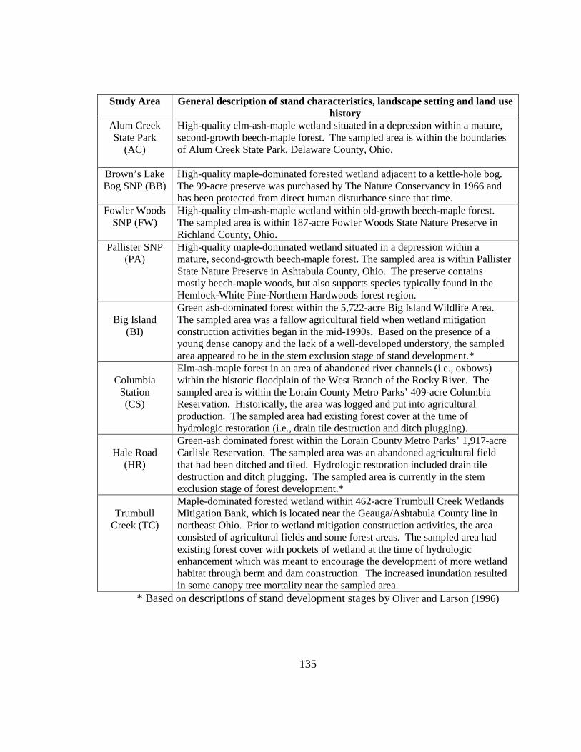
135
Study Area General description of stand characteristics, landscape setting and land use history
Alum Creek State Park
(AC)
High-quality elm-ash-maple wetland situated in a depression within a mature, second-growth beech-maple forest. The sampled area is within the boundaries of Alum Creek State Park, Delaware County, Ohio.
Brown’s Lake Bog SNP (BB)
High-quality maple-dominated forested wetland adjacent to a kettle-hole bog. The 99-acre preserve was purchased by The Nature Conservancy in 1966 and has been protected from direct human disturbance since that time.
Fowler Woods SNP (FW)
High-quality elm-ash-maple wetland within old-growth beech-maple forest. The sampled area is within 187-acre Fowler Woods State Nature Preserve in Richland County, Ohio.
Pallister SNP (PA)
High-quality maple-dominated wetland situated in a depression within a mature, second-growth beech-maple forest. The sampled area is within Pallister State Nature Preserve in Ashtabula County, Ohio. The preserve contains mostly beech-maple woods, but also supports species typically found in the Hemlock-White Pine-Northern Hardwoods forest region.
Big Island
(BI)
Green ash-dominated forest within the 5,722-acre Big Island Wildlife Area. The sampled area was a fallow agricultural field when wetland mitigation construction activities began in the mid-1990s. Based on the presence of a young dense canopy and the lack of a well-developed understory, the sampled area appeared to be in the stem exclusion stage of stand development.*
Columbia
Station (CS)
Elm-ash-maple forest in an area of abandoned river channels (i.e., oxbows) within the historic floodplain of the West Branch of the Rocky River. The sampled area is within the Lorain County Metro Parks’ 409-acre Columbia Reservation. Historically, the area was logged and put into agricultural production. The sampled area had existing forest cover at the time of hydrologic restoration (i.e., drain tile destruction and ditch plugging).
Hale Road
(HR)
Green-ash dominated forest within the Lorain County Metro Parks’ 1,917-acre Carlisle Reservation. The sampled area was an abandoned agricultural field that had been ditched and tiled. Hydrologic restoration included drain tile destruction and ditch plugging. The sampled area is currently in the stem exclusion stage of forest development.*
Trumbull
Creek (TC)
Maple-dominated forested wetland within 462-acre Trumbull Creek Wetlands Mitigation Bank, which is located near the Geauga/Ashtabula County line in northeast Ohio. Prior to wetland mitigation construction activities, the area consisted of agricultural fields and some forest areas. The sampled area had existing forest cover with pockets of wetland at the time of hydrologic enhancement which was meant to encourage the development of more wetland habitat through berm and dam construction. The increased inundation resulted in some canopy tree mortality near the sampled area.
* Based on descriptions of stand development stages by Oliver and Larson (1996)