Krishnakumar Rajagopalan

Gerard C. Nihous1

e-mail: nihous@hawaii.edu

Department of Ocean and

Resources Engineering,

University of Hawaii,

Honolulu, HI 96822

An Assessment of GlobalOcean Thermal EnergyConversion Resources Witha High-Resolution OceanGeneral Circulation ModelGlobal rates of ocean thermal energy conversion (OTEC) are assessed with a high-resolution (1 deg� 1 deg) ocean general circulation model (OGCM). In numerically in-tensive simulations, the OTEC process is represented by a pair of sinks and a source ofspecified strengths placed at selected water depths across the oceanic region favorablefor OTEC. Results broadly confirm earlier estimates obtained with a coarse(4 deg� 4 deg) OGCM, but with the greater resolution and more elaborate description ofkey physical oceanic mechanisms in the present case, the massive deployment of OTECsystems appears to affect the global environment to a relatively greater extent. The maxi-mum global OTEC power production drops to 14 TW, or about half of previously esti-mated levels, but it would be achieved with only one-third as many OTEC systems.Environmental effects at maximum OTEC power production are generally similar in bothsets of simulations. The oceanic surface layer would cool down in tropical OTEC regionswith a compensating warming trend elsewhere. Some heat would penetrate the ocean in-terior until the environment reaches a new steady state. A significant boost of the oceanicthermohaline circulation (THC) would occur. Although all simulations with given OTECflow singularities were run for 1000 years to ensure stabilization of the system, conver-gence to a new equilibrium was generally achieved much faster, i.e., roughly within acentury. With more limited OTEC scenarios, a global OTEC power production of theorder of 7 TW could still be achieved without much effect on ocean temperatures. [DOI:10.1115/1.4023868]

Keywords: ocean thermal energy conversion (OTEC), ocean general circulation model

1 Introduction

Ocean thermal energy conversion has long held the promise ofproviding mankind with vast amounts of renewable electricalpower [1,2]. The concept is based on a heat engine operatingbetween a warm reservoir consisting of surface seawater and acold reservoir consisting of deep seawater. Obviously, OTECwould work in areas with a strong and stable thermal stratificationof the oceanic water column, i.e., generally within tropicallatitudes. While the idea is simple enough, practical seawater tem-perature differences are not great (�20 �C) so that OTEC cyclesrequire relatively large seawater flow rates, of the order of severalcubic meters per second per megawatt of net electricity produced.This and other difficulties typical of deepwater marine environ-ments have prevented OTEC from being commercially imple-mented so far. A growing worldwide energy demand coupled withthe prospect of declining fossil fuel reserves and serious concernsabout climate change could, however, make this technology com-petitive in a not too distant future. More details regarding OTECcan easily be found in the technical literature [3].

With past efforts focused on practical engineering challenges,the size of the global OTEC resource understandably has not beenan urgent concern. This has led to a wide range of estimates given,more often than not, with little justification and a tendency to

exaggerate [4]. A key issue highlighted in a series of early model-ing studies [4–6] is whether or not OTEC seawater flow ratescould affect the thermal stratification of the ocean on which theprocess depends. Since OTEC net power production is a very sen-sitive function of the available thermal resource, of the order of15% per 1 �C, a very dense deployment of OTEC systems mightbe self-limiting. Under this scenario, OTEC resources wouldactually have a maximum. This was shown in simple one-dimensional models of the water column with OTEC [4–6], whereit was also suggested that the environmental rate of deep waterformation was a natural scale for cold seawater globally used inOTEC plants.

More recently, the question of global OTEC resource wastackled for the first time with state-of-the-art ocean general circu-lation models [7]. A relatively coarse numerical grid was adoptedto limit the numerical burden of the proposed simulations, i.e.,(4 deg� 4 deg) horizontally with 15 vertical layers including a50 m thick surface layer. The existence of a maximum for globalOTEC net power production was confirmed. At 30 TW, thismaximum would be about ten times that predicted in earlier one-dimensional studies [4,5]. Such a result demonstrated the impor-tance of fast horizontal transport phenomena, not accounted for inone-dimensional models, in slowing the local erosion of the watercolumn’s thermal stratification as OTEC flow intensity increases.It was also revealed that a cooling of the surface layer in theOTEC region could be sustained as long as warming occurs else-where [7]. Although this work represents an important step tomore accurately assess interactions between the environment anda very large number of OTEC systems deployed throughout the

1Corresponding author.Contributed by the Advanced Energy Systems Division of ASME for publication

in the JOURNAL OF ENERGY RESOURCES TECHNOLOGY. Manuscript received January 1,2013; final manuscript received February 12, 2013; published online May 31, 2013.Assoc. Editor: Kau-Fui Wong.

Journal of Energy Resources Technology DECEMBER 2013, Vol. 135 / 041202-1Copyright VC 2013 by ASME

Downloaded From: http://energyresources.asmedigitalcollection.asme.org/ on 07/01/2013 Terms of Use: http://asme.org/terms

tropical seas, significant improvements in OGCM computationaland physical resolutions are proposed in the present study. Thesimulation procedure is described in the next section before resultsare presented and discussed.

2 Methodology

2.1 Description of Ocean General Circulation Model. Theocean general circulation model MITgcm was selected for thisstudy [8,9]. This open-source numerical code was also adopted inprevious coarse-resolution simulations of global OTEC resources[7]. Discretized transport equations for momentum, potentialtemperature, and salinity are solved using a finite-volume tech-nique. A key capability of recent versions of MITgcm, in order torepresent OTEC processes, is an option to imbed fluid sources inthe domain, as explained in Sec. 2.3 below. Necessary butstraightforward modifications to allow fluid sinks were imple-mented as well [7]. A detailed description of MITgcm is beyondthe scope of this article and is available elsewhere [8,9].

The numerical resolution targeted in this study is 1 deg� 1 deghorizontally with 23 vertical layers of thicknesses, starting fromthe top, in meters: 10, 10, 15, 20, 20, 25, 35, 50, 75, 100, 150,200, 275, 350, 415, 450, 500, 500, 500, 500, 500, 500, and 500.The choice of thinner layers toward the surface allows a betterrepresentation of enhanced vertical stratification in the upper partof the water column. Model setup generally follows that of Forget[10]. In particular, the time step is one hour for the tracer equa-tions (temperature and salinity), and 10 min for the momentumequations (staggered baroclinic time stepping). In the presentstudy, sea ice is not explicitly modeled and ice covered regionsare considered as land. Seawater temperature is not allowed todrop below the ice point (��2 �C), however, and this condition isenforced through compensating heat fluxes. Some key input fileslike bathymetry and initial tracer fields were also available fromthe ECCO (Estimating the Circulation and the Climate of theOcean) Group2.

The model is forced with several monthly averaged fluxesspecified at the ocean-atmosphere boundary. Meridional and zonalwind-stress fields were obtained from a well-known data base[11]. The other input consists of heat, short-wave radiation, andfreshwater fluxes. Their specification required a delicate two-stepprocess. At first, essential flux components were either directlyfound or determined from extensive parameterizations [11–13];these include the short-wave radiation, long-wave radiation, latentheat, sensible heat, evaporation, and precipitation fluxes. Some in-termediate fields were available elsewhere, such as the short-waveradiation under clear skies3 and the surface albedo4. In our simula-tions, two important constraints had to be satisfied for the OGCMto run properly: that the annual averages of the heat and fresh-water fluxes integrated over the entire ocean surface both be zero.Simply using available or calculated data generally fails toapproximate such constraints to an acceptable degree. In theabsence of continuous data assimilation, small inaccuracies in sur-face input fluxes can lead to large drifts in calculated fields overlong enough simulation times, a point discussed in Sec. 2.2. Themethodology adopted here was to multiply key terms in the heatand freshwater fluxes by unknown tuning parameters (of orderone) [11]. The seven selected parameters were then determined byminimizing the normalized sum of the yearly averaged heat andfreshwater fluxes integrated over the entire ocean surface. Thisoperation was performed with a standard multidimensionaldownhill simplex method implemented in the MATLAB

VR

functionfminsearch. A low threshold of 0.9 was also imposed on the tun-ing parameters, which ended up ranging from 0.91 to 1.09.

Coupling between the atmosphere and the ocean is accom-plished using local relaxation terms. In this simple formalism, the

atmosphere itself is not modeled and the ocean linearly respondsto perturbations expressed as deviations of calculated oceansurface values (temperature or salinity) from set references. Thereference fields were chosen from data [11] at the same depth asthe middle of the first model layer. In the case of temperature, therelaxation proportionality coefficients were evaluated from first-order analytical expansions of the surface heat fluxes around thereference values [14]. There is no such physical justification inthe case of salinity since salinity relaxation is only a convenientbut necessary computational artifact. It prevents the calculatedsalinity field from excessive drift due to inaccuracies in the pre-cipitation forcing [15]. A relaxation time scale of one month waschosen from a comparable model setup [16]. It must be empha-sized that a cure for problems arising with ocean-atmosphere cou-pling in OGCMs would be to run fully coupled ocean-atmospheresimulations. This represents a difficult task, but it might be worthattempting in the future when considering global OTEC scenarioswhere heat exchange at the ocean-atmosphere plays a key role.

2.2 Basic OGCM Calibration Tests. MITgcm as describedearlier was run for 1000 model years to ensure an adequatestabilization of calculated fields (i.e., a quasi steady state of yearlyaveraged variables and a reproduction of seasonal variability). Itwas first verified that the global heat and salt budgets were closed,i.e., that cumulative external additions matched the net cumulativechange in the ocean interior. External additions include boundaryfluxes as well as the heat added to seawater to prevent it fromcooling below the ice point.

Next, the issue of temperature and salinity drift was considered.To this effect, globally-integrated yearly-averaged temperatureand salinity were tracked as a function of time (global integrationin the fluid domain uses the volumes of computational cells asweights). The coordinated ocean-ice reference experiments(COREs) model inter-comparison study was used as a benchmark[15]. After 500 years, global temperature drifted from an initialvalue of 3.65 �C to 3.42 �C. More importantly, it leveled off after200 years or so. Among the predictions from the seven OGCMSdiscussed in COREs, only two sets exhibit better global tempera-ture drift characteristics than the present simulations [15]. At theend of the 1000 year spin-up time, the global temperature drift inthe (1 deg� 1 deg) calculations was more than three times smallerthan with the (4 deg� 4 deg) model setup [7]. Global salinityexhibited a small linear trend of 0.006 psu per century (i.e., lessthan 0.02% per century) but with no sign of better stabilization atthe end of the spin-up period. Surprisingly, the coarser model hadfared better with global salinity reaching a plateau after 200 yearsor so, at a level comparable to the value reached after 400 years(but growing) in the higher-resolution simulations. Among theCOREs predictions, five out of seven sets display better global sa-linity drift characteristics than the present simulations. Overall,however, the stability of predictions from MITgcm as configuredfor this study is excellent. It compares well with the performanceof other state-of-the-art OGCMs [15] and provides a more stabletemperature field than its coarser predecessor [7].

A meaningful test often used by ocean modelers concerns theglobal thermohaline circulation (THC), more accurately referredto as meridional overturning circulation (MOC) since mechanicalforcing (e.g., from wind stress) cannot be separated from thermo-haline effects (density differences). The THC represents the net-work of slow planetary currents, which effectively transports deepwater, formed at a few selected high-latitude spots, throughoutmost ocean basins. Coincidentally, the THC makes OTEC possi-ble in tropical regions by supplying and replenishing deep coldseawater there. Following a typical methodology [17], a parallelin the North Atlantic is selected, e.g., 26 deg N, across which ve-locity is integrated across all meridians in each vertical layer. Thisyields zonal integrals (in units of volume flow rate) correspondingto each layer. Yearly-averaged results from such calculations areshown in Fig. 1 for the present model setup at the end of the 1000

2For more information, visit http://www.ecco-group.org/products.htm.3For more information, visit http://eosweb.larc.nasa.gov/sse/.4For more information, visit http://www-cave.larc.nasa.gov/cave/avg/.

041202-2 / Vol. 135, DECEMBER 2013 Transactions of the ASME

Downloaded From: http://energyresources.asmedigitalcollection.asme.org/ on 07/01/2013 Terms of Use: http://asme.org/terms

year spin-up time; also displayed are published time-mean OGCMpredictions using 12 year historical forcing (1992–2004) and dataassimilation [17]. By convention, northward flow is positive.Overall, predicted zonal-integral profiles have the same shape.The synoptic MITgcm predictions appear shifted slightly upward,but a one-to-one comparison would be difficult since there aresignificant differences between simulation protocols. One metricfor the THC strength can be obtained by adding the upper-oceanpositive values of the zonal integrals. This yields 11.4 Sv versus13.2 Sv in Wunsch and Heimbach [17], where an uncertainty of61.8 Sv is suggested (1 Sv¼ 106 m3 s�1). The same procedurefrom coarser (4 deg� 4 deg) resolution MITgcm simulationsyielded 14.9 Sv [7]. Other published studies based on hydro-graphic data and models using inverse methods report estimatesof about 16 6 2 Sv at about the same latitude [18,19]. Althoughthe THC strength estimated from (1 deg� 1 deg) resolutionMITgcm predictions seems a little low, it remains well within ac-ceptable uncertainties when comparing the performance of differ-ent OGCMs [15].

2.3 OTEC Simulations. The OTEC region is defined wheremonthly average seawater temperature differences between 20 mand 1000 m water depths never drop below 18 �C. Essentiallylocated between 30�N and 30�S, it covers an area of about114� 106 square kilometers or roughly one-third of the ocean.The reference data base is the quarter-degree World Ocean Atlas2005 [20]. Due to the high cost of large submarine power cablesover long distances, the potential development of remote offshoreOTEC resources has often been linked to the emergence of futurehydrogen based economies [21].

At a given location, the OTEC net power area density Pnet canbe calculated from the following simple formulas adapted fromearlier studies [4,5]:

Pnet ¼ wcw3qcpetgc

16ð1þ cÞðDTÞ2

T� Ppump (1)

Ppump ¼ wcw0:30qcpetgc

4ð1þ cÞ (2)

In Eq. (1), wcw is the volume flow rate of the deep seawater intakeper unit (latitude-longitude) area and has the dimension of avelocity. c is the flow rate ratio of the surface seawater intake overthe deep seawater intake; it is fixed throughout this study andequal to 1.5, a value typical of optimized floating OTEC systems.T is the absolute temperature of the OTEC surface seawaterintake, and DT is the temperature difference between surface and

deep seawater intakes. The pumping power density defined inEq. (2) corresponds to 30% of the first term in the right-hand-sideof Eq. (1) (gross power density) taken at standard conditionsDT¼ 20 �C and T¼ 300 K. The average seawater density q istaken as 1025 kg m�3, the seawater specific enthalpy cp as4000 J kg�1 K�1, and the OTEC combined turbo-generator effi-ciency etg as 0.75. Despite their simplicity, the proposed powerformulas capture the basic behavior of OTEC systems based onpure-fluid, low temperature Rankine cycles, with thermodynamicefficiencies approximately half the Carnot limit of DT over T. Ifmore complex cycles were considered, e.g., of the Kalina type[22], Eqs. (1) and (2) should be modified accordingly.

Each OTEC simulation (scenario) is defined by a fixed valueof wcw. Multiplying wcw by the horizontal areas of MITgcmnumerical grid cells throughout the OTEC region defines a field ofdeep seawater fluid sinks Qcw located in the 14th vertical layer, ata water depth of 1160 m (cell midpoint). The OTEC surface sea-water sinks Qww, simply equal to c times Qcw, are placed in the 3rd

vertical layer at a water depth of 27.5 m (cell midpoint). A sourceof strength (QwwþQcw) represents the mixed effluents of theOTEC process. Because of the very small conversion rate of ther-mal energy in OTEC systems, the effluent temperature iscalculated from those of the two intakes with a simple mixingrule. The same procedure is adopted to determine effluent salinity.Following earlier modeling protocols [4–7], the vertical locationof the effluent source is selected where it would be neutrally buoy-ant just before OTEC flow singularities are turned on in themodel. Given limitations from the numerical discretization of thewater column, this yields discharge water depths of the order of50–250 m throughout the OTEC region, i.e., generally greaterthan in actual systems for which economical constraints would bestrong. The rationale for this arbitrary choice is to minimize thebuoyant mixing and sinking of heavier (colder) effluents beforethey reach a level of neutral buoyancy.

It must be emphasized that a global (1 deg� 1 deg) oceanmodel with 23 vertical layers remains too coarse if one were inter-ested in detailed simulations, for example, involving mesoscaleoceanic eddies. Pushing this thought further, the OTEC scenariosdefined here are too crude to allow the realistic simulations ofphenomena taking place at very small subgrid scales. This moti-vates the present lack of focus on the buoyancy-driven settling ofOTEC effluents. It also justifies running MITgcm in its simpler,numerically more efficient hydrostatic formulation, where theequation of conservation of vertical momentum is reduced to ahydrostatic pressure balance, and vertical velocities are deter-mined from mass conservation. Accordingly, no momentum isassigned to the OTEC effluent source.

OTEC net power is determined from Eqs. (1) and (2) usingseawater temperatures predicted by MITgcm for given OTEC sce-narios. Even though the present model setup produces limitedtemperature drift, as discussed in Sec. 2.2, the sensitivity ofOTEC power to temperature (and the whole emphasis of thisstudy) requires particular care. Therefore, temperatures in Eq. (1)are equal to their initial values augmented by the calculated tem-perature changes from the end of model spin-up (1000 years) toany given time following the onset of OTEC operations.

3 Results and Discussion

Figure 2 shows the long-term yearly averaged global OTECpower as a function of OTEC flow intensity wcw (m yr�1), after1000 years of OTEC operations. The zero-feedback curves aresteep straight lines that reflect the linearity of power as a functionof wcw, embodied in Eqs. (1) and (2), if ocean temperatures didnot change; the very slight differences for different horizontal-grid resolutions stem from minor area adjustments of the OTECregion to conform to either numerical grid. With the high-resolution OGCM, global OTEC power is predicted to reach amaximum of 14 TW when wcw¼ 20 m yr�1. This contrasts sharplywith earlier estimates from the coarser model. The revised OTEC

Fig. 1 26�N zonal integrals of the North Atlantic velocityfields multiplied by the appropriate layer thicknesses (Sv) as afunction of depth (m): MITgcm calculations are yearly averagesafter 1000-year spin-up (this work); other results are 1992–2004time means under data constraints [17]

Journal of Energy Resources Technology DECEMBER 2013, Vol. 135 / 041202-3

Downloaded From: http://energyresources.asmedigitalcollection.asme.org/ on 07/01/2013 Terms of Use: http://asme.org/terms

power limit is roughly half the previous value, but it is achievedwith an OTEC flow intensity only one-third as large. In truth, thisdoes not mean that OTEC systems are predicted to be more“efficient” in higher-resolution simulations; instead, it reflects thefact that in all simulations, OTEC systems experience less adverseseawater temperature feedback at lower values of wcw. The overallOTEC flow rates involved are considerable, and of the same orderof magnitude as large components of the global oceanic circula-tion (wcw¼ 20 m yr�1 corresponds to 72 Sv).

To get a sense of the number of actual OTEC plants that wouldcorrespond to a given OTEC flow intensity wcw, the simplest waywould be to divide the corresponding zero-feedback power inFig. 2 by a nominal plant size (100 MW is broadly considered to bea single-unit commercial target given technological limitations onthe deep cold seawater pipe size). Since power production withgiven hardware is dependent on local conditions, however, it wouldbe more consistent to assign the nominal commercial plant a givendeep seawater flow rate. One would then multiply wcw by the areaof the OTEC region and divide this overall deep seawater intakeflow rate by the reference value, such as 300 m3 s�1 per 100 MWsystem (rated at typical, fixed seawater temperatures). For example,with wcw¼ 20 m yr�1 when long-term global OTEC power produc-tion would peak, the first method would yield 330,000 plantswhereas the second would correspond to 240,000 plants. On the av-erage, though, it can be said that if deployed together, those systemswould effectively lose about half of their power rating from adversefeedback on the seawater temperature field.

Given the significant differences between simulationsattempted at two different numerical resolutions with the sameOGCM, in previous work [7] and in the present study, it is legiti-mate to wonder whether results from the higher-resolution versionhave numerically converged. A definite answer would requiresimulations to be performed at resolutions greater than(1 deg� 1 deg) horizontally, with more than the 23 vertical layerscurrently selected. This could be done in the future but is not easy.To be consistent, reliable input forcing files (wind stress, surfaceheat, etc.) would have to be produced at a resolution compatiblewith the improved numerical grid. Adequate computing capabil-ities would then be required. In the present study, a single OTECsimulation over 1000 years takes about 1 week on 64 parallel pro-cessors (CPUs). Just doubling the overall grid resolution (horizon-tally and vertically) would increase the number of numerical cellsby a factor of 8. In doing so, however, the time step also wouldhave to be reduced to ensure numerical stability. To give a senseof the task, the published calculations performed with the 15-layer, (4 deg� 4 deg) MITgcm setup were more than 100 timesfaster than those presented here [7]. There is more to distinguishthe two model versions than numerical resolution, however. Someimportant physical features are represented in the high-resolutionversion, such as the Mediterranean Sea, which has a significant

influence on the temperature and salinity fields of the NorthAtlantic. With several thinner surface layers instead of a single50 m thick top layer, the K-profile parameterization (KPP) optionof Large et al. [23] is used here to better describe the surfaceboundary layer and determine vertical mixing in the criticaltopmost section of the water column. In particular, the input ofshort-wave solar radiation at the ocean surface and subsequentabsorption in the topmost layers are explicitly treated. Hence, thepresent calculations should be considered better than earlier esti-mates from both numerical and physical points of view. Also, it isvery unlikely that greater-resolution results would get close to the1D predictions also shown in Fig. 2 [5]. Horizontal transport phe-nomena are orders of magnitude faster in the ocean (in reality,and as modeled in OGCMs). It is, therefore, reasonable to expectOTEC feedbacks on the temperature structure of the water columnto be substantially amplified in a 1D model where horizontaladvection and diffusion are not included.

Even though the OTEC scenarios implemented in this study aremerely numerical experiments, the response of the environment insuch simulations provides valuable information. It is important,for example, to get a sense of the time scales involved in the tran-sition between an ocean without OTEC and an ocean that hasreached a new equilibrium for a given OTEC scenario. Figure 3shows how the yearly averaged global OTEC power evolves forvarious OTEC flow intensities (only up to wcw¼ 40 m yr�1 forreadability). A noticeable feature of all curves is a steep initialdrop in power output over a period as short as about five years.This effect prevails over the entire range of simulated OTEC flowintensities wcw, from 5 m yr�1 to 80 m yr�1. In fact, a drop ofabout 0.6% to 0.7% per (m yr�1) is consistently predicted. Such arapid and general phenomenon could only involve fast mecha-nisms that respond somewhat proportionately to the stepwiseonset of OTEC flows. Hence, modifications of the global oceancirculation as well as any heat input that would affect the OTECdeep seawater intake temperature have to be ruled out as causallinks. The temperature across the ocean surface layers respondslocally and quickly wherever OTEC operations are included, apoint that was apparent even in earlier one-dimensional analyses[5]. It is, therefore, the local cooling effect of OTEC operations inthe upper layer of the ocean that induces the initial drop in pre-dicted OTEC power. What follows is slower and more complex,but eventually results in a warming of the OTEC deep seawaterintake layer. Overall, all scenarios practically reach a new equilib-rium within a century or so. As OTEC flow intensities wcw

increase above 20 m yr�1, long-term global OTEC power outputsdecrease as shown in Fig. 2. It is clear, then, that the more massiveOTEC scenarios would cause dramatic changes in the oceanicenvironment; in turn, this would cause corresponding OTEC

Fig. 2 Long-term (1000 year) yearly averaged global OTECpower as a function of OTEC flow intensity wcw (m yr21)

Fig. 3 Yearly averaged global OTEC power as a function oftime for different OTEC flow intensities wcw (m yr21)

041202-4 / Vol. 135, DECEMBER 2013 Transactions of the ASME

Downloaded From: http://energyresources.asmedigitalcollection.asme.org/ on 07/01/2013 Terms of Use: http://asme.org/terms

power production to plummet from high zero-interaction values todismal levels.

The potential erosion of OTEC resources with the implementa-tion of widespread massive OTEC operations is geographicallyvariable, too. Figure 4, plotted with the Ocean Data View software[24], gives selected time plots of OTEC net power density whenglobal output is maximal (wcw¼ 20 m yr�1). Some areas appear to

fare relatively worse than others, e.g., in the Indian Ocean andalong the Equator. In some locations, net power production wouldessentially cease. When the new equilibrium is reached, the high-est OTEC net power density is seen off of Brazil rather than in thetropical Western Pacific.

More generally, OTEC flows can impact oceanic regions thatlie outside of the OTEC zone. For example, an ocean surface

Fig. 4 Variation of yearly averaged OTEC power density (kW m22) when wcw 5 20 m yr21. (a) Initial field (no feedback from OTECplants), (b) 5 year feedback, (c) 25-year feedback, (d) 50 year feedback, (e) 100 year feedback, and (f) 200 year (nearly asymptotic)feedback.

Journal of Energy Resources Technology DECEMBER 2013, Vol. 135 / 041202-5

Downloaded From: http://energyresources.asmedigitalcollection.asme.org/ on 07/01/2013 Terms of Use: http://asme.org/terms

cooling in areas of large-scale OTEC deployment has long beenpostulated [25,26]. It was later demonstrated in simple one-dimensional models [4–6], but only as a transient phenomenon.An important difference between such limited analyses and three-dimensional simulations was highlighted with OGCM coarse-gridcalculations [7]: the long-term (equilibrium) temperature of theocean surface layer is not constrained to its pre-OTEC value. In

other words, an OTEC-induced cooling of the surface layer in theOTEC region can be sustained as long as some warming occurselsewhere, such that the overall heat flux between the ocean andthe atmosphere eventually returns to zero (since there is no“elsewhere” in a one-dimensional model, an equilibrium heat fluxof zero at the top of the water column becomes a temperaturerequirement). Figures 5 and 6, plotted with the Ocean Data View

Fig. 4 Variation of yearly averaged OTEC power density (kW m22) when wcw 5 20 m yr21. (a) Initial field (no feedback from OTECplants), (b) 5 year feedback, (c) 25-year feedback, (d) 50 year feedback, (e) 100 year feedback, and (f) 200 year (nearly asymptotic)feedback.

041202-6 / Vol. 135, DECEMBER 2013 Transactions of the ASME

Downloaded From: http://energyresources.asmedigitalcollection.asme.org/ on 07/01/2013 Terms of Use: http://asme.org/terms

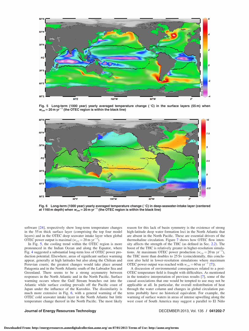
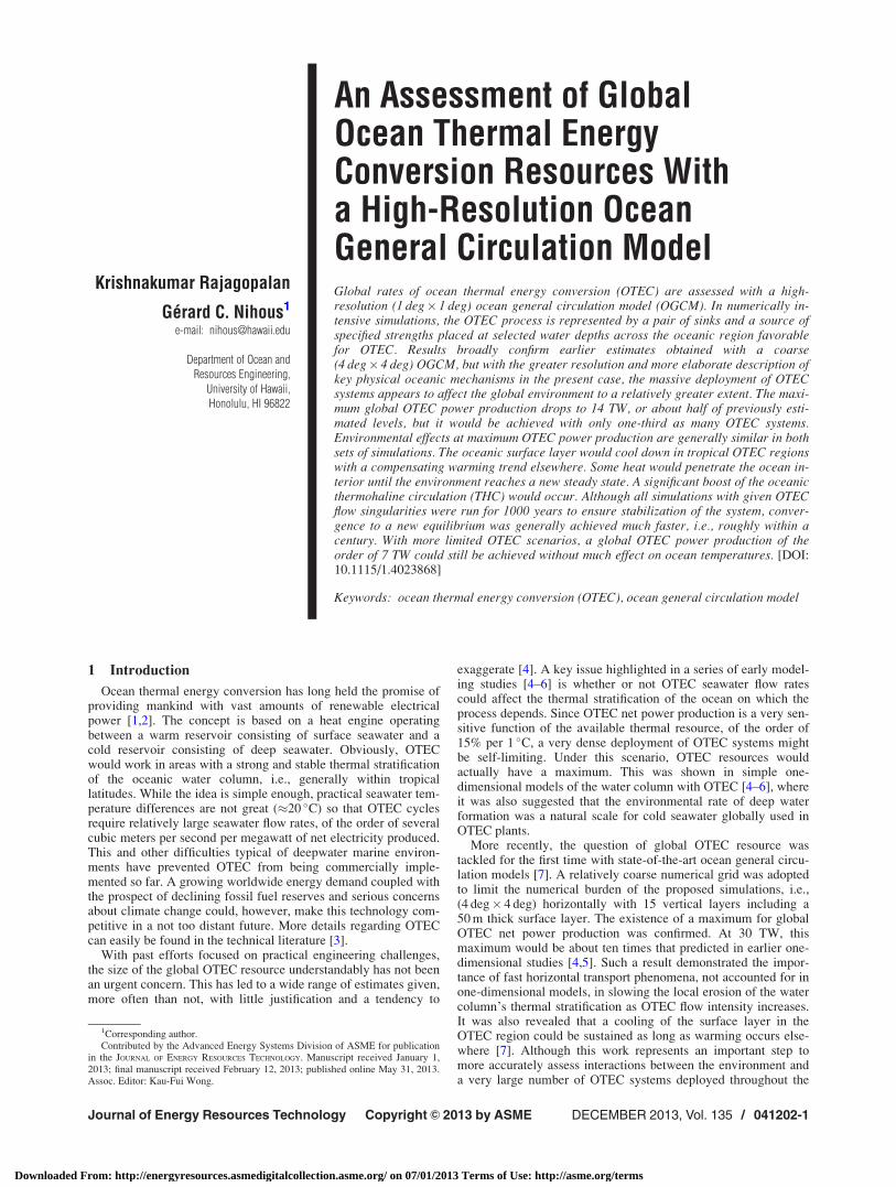
software [24], respectively show long-term temperature changesin the 55 m thick surface layer (comprising the top four modellayers) and in the OTEC deep seawater intake layer when globalOTEC power output is maximal (wcw¼ 20 m yr�1).

In Fig. 5, the cooling trend within the OTEC region is morepronounced in the Indian Ocean and along the Equator, whereFig. 4 suggested a substantial long-term loss of OTEC power pro-duction potential. Elsewhere, areas of significant surface warmingappear, generally at high latitudes but also along the Chilean andPeruvian coasts; the greatest changes would take place aroundPatagonia and in the North Atlantic south of the Labrador Sea andGreenland. There seems to be a strong asymmetry betweenresponses in the North Atlantic and in the North Pacific. Surfacewarming occurs where the Gulf Stream branches out into theAtlantic while surface cooling prevails off the Pacific coast ofJapan under the influence of the Kuroshio. The dissimilarity ismuch more extensive in Fig. 6, with a general warming of theOTEC cold seawater intake layer in the North Atlantic but littletemperature change thereof in the North Pacific. The most likely

reason for this lack of basin symmetry is the existence of stronghigh-latitude deep water formation loci in the North Atlantic thatare absent in the North Pacific. These are essential drivers of thethermohaline circulation. Figure 7 shows how OTEC flow inten-sity affects the strength of the THC (as defined in Sec. 2.2). Theboost of the THC is relatively greater in higher-resolution simula-tions. At maximum OTEC power production (wcw¼ 20 m yr�1),the THC more than doubles to 25 Sv (coincidentally, this conclu-sion also held in lower-resolution simulations where maximumOTEC power output was reached with wcw¼ 60 m yr�1 [7]).

A discussion of environmental consequences related to a post-OTEC temperature field is fraught with difficulties. As mentionedin the tentative interpretation of previous results [7], some of thecausal associations that one would be tempted to use may not beapplicable at all. In particular, the overall redistribution of heatthrough the water column and changes in global circulation pat-terns probably have no historical equivalent. For example, thewarming of surface waters in areas of intense upwelling along thewest coast of South America may suggest a parallel to El Nino

Fig. 5 Long-term (1000 year) yearly averaged temperature change ( �C) in the surface layers (55 m) whenwcw 5 20 m yr21 (the OTEC region is within the black line)

Fig. 6 Long-term (1000 year) yearly averaged temperature change ( �C) in deep-seawater-intake layer (centeredat 1160 m depth) when wcw 5 20 m yr21 (the OTEC region is within the black line)

Journal of Energy Resources Technology DECEMBER 2013, Vol. 135 / 041202-7

Downloaded From: http://energyresources.asmedigitalcollection.asme.org/ on 07/01/2013 Terms of Use: http://asme.org/terms

events, but the mechanisms involved are very different. Importantmodel limitations also invite care to avoid over-interpretation. Toinfer any conclusion of a climatic nature, modeling of the atmos-phere with a full coupling to the ocean would be warranted. If onewere to adopt a precautionary principle, however, an ocean sur-face warming of several degrees south of Greenland would not bewelcome given current concerns about climate change. Eventhough large OTEC scenarios implemented stepwise have essen-tially no chance to take place (except in numerical experiments),one could use the predicted ocean surface warming at a criticallocation to suggest some OTEC power production threshold. Onthe basis of Fig. 8, a previous argument that an overall globalOTEC power output of the order of 7 TW achieved withwcw¼ 5 m yr�1 would be acceptable from an environmental per-spective [7] seems to hold, despite the greater sensitivity of theresults in higher-resolution calculations. Finally, it must be men-tioned that all OTEC simulations are reversible. When turning offthe prescribed OTEC sources and sinks in the model, the environ-ment is shown to relax to its pre-OTEC condition. The time scalesfor both reverse and direct processes are similar (e.g., as shown inFig. 4 when wcw¼ 20 m yr�1).

4 Conclusions

Global rates of ocean thermal energy conversion were esti-mated with a high-resolution configuration of the ocean generalcirculation model MITgcm. The (1 deg� 1 deg) horizontal globalgrid with 23 vertical layers resulted in numerically intensive simu-lations but allowed a better representation of important physicalphenomena (e.g., Mediterranean outflow, mixed layer scheme[23]). As in previous studies [4–7], the OTEC process wasreduced to a pair of intake sinks and an effluent source of specifiedstrengths placed at selected water depths across the oceanic regionfavorable for OTEC.

Results broadly confirmed earlier estimates obtained with acoarse (4 deg� 4 deg), 15-layer OGCM [7]. In the present case,however, the massive deployment of OTEC systems appeared toaffect the global environment to a relatively greater extent. Thepredicted maximum global OTEC power production reached 14TW or about half of previously estimated levels [7]. Such anoutput remains comparable to mankind’s current consumption ofprimary energy. It would be achieved with only one-third as manyOTEC systems (wcw¼ 20 m yr�1) as previously estimated [7].This apparent efficiency improvement merely reflects the fact that

Fig. 8 Long-term (1000 year) yearly averaged temperature change (�C) in thesurface layers (50 or 55 m) at 58�N, 46�W as a function of OTEC flow intensity wcw

(m yr21)

Fig. 7 Long-term (1000 year) yearly averaged strength of the Atlantic thermoha-line circulation (Sv) as a function of OTEC flow intensity wcw (m yr21)

041202-8 / Vol. 135, DECEMBER 2013 Transactions of the ASME

Downloaded From: http://energyresources.asmedigitalcollection.asme.org/ on 07/01/2013 Terms of Use: http://asme.org/terms

in all simulations, less adverse seawater temperature feedbackoccurs when fewer plants are deployed (lower values of wcw). Theoverall OTEC flow rates under consideration remain very signifi-cant, since wcw¼ 20 m yr�1 is equivalent to 72 Sv. This typicallywould correspond to the operation of a quarter million largeOTEC plants (rated at 100 MW in standard conditions). Withmore limited OTEC scenarios, a global OTEC power productionof the order of 7 TW could still be achieved without much effecton ocean temperatures.

Although all simulations with given OTEC flow singularitieswere run for 1000 years to ensure stabilization of the system, con-vergence to a new equilibrium was generally achieved muchfaster, i.e., roughly within a century. Environmental effects atmaximum OTEC power production were qualitatively similar to,but quantitatively more acute than, those reported earlier [7]. Theoceanic surface layer was shown to cool down in tropical OTECregions, with a compensating warming trend elsewhere. Someheat would penetrate the ocean interior until the environmentreaches a new steady state. A significant boost of the oceanic ther-mohaline circulation would occur.

Although the use of OGCMs clearly is a method of choice toestimate global OTEC resources, much work remains to be doneto gain confidence in the results obtained so far. This is high-lighted by notable differences between the present study andearlier work [7]. It is debatable whether numerically costlyimprovements in grid resolution should be attempted first. Instead,a better physical representation of the coupling between the oceanand the atmosphere may yield more valuable insights, although itwould also involve a significant effort. A crude definition of wide-spread, abruptly implemented OTEC scenarios lends itself torefinements as well, perhaps with some practical OTEC deploy-ment roadmap as a basis. Whether and how the development ofOTEC proceeds, however, may depend on a paradigm shift in theevaluation of all power production systems [27].

Acknowledgment

This research was funded by a grant from the U.S. Departmentof Energy through the Hawaii National Marine Renewable EnergyCenter{FundingSource} (Hawaii Natural Energy Institute, Uni-versity of Hawaii). Computer simulations were done, in part andfree of charge, at the Hawaii Open Supercomputing Center(HOSC) operated by the Maui High Performance Computing Cen-ter (MHPCC).

References[1] d’Arsonval, A., 1881, “Utilisation des forces naturelles. Avenir de l’Electricite,”

Rev. Sci., 17, pp. 370–372, in French, available at: http://gallica.bnf.fr/ark:/12148/bpt6k215097r

[2] Claude, G., 1930, “Power From the Tropical Seas,” Mech. Eng., 52(12), pp.1039–1044.

[3] Avery, W. H., and Wu, C., 1994, Renewable Energy From the Ocean—A Guideto OTEC, Johns Hopkins University Applied Physics Laboratory Series inScience and Engineering, J. R. Apel, ed., Oxford University Press, New York,p. 446.

[4] Nihous, G. C., 2005, “An Order-Of-Magnitude Estimate of Ocean ThermalEnergy Conversion Resources,” ASME J. Energy Res. Technol., 127, pp.328–333.

[5] Nihous, G. C., 2007, “A Preliminary Assessment of Ocean Thermal EnergyConversion (OTEC) Resources,” ASME J. Energy Res. Technol., 129, pp.10–17.

[6] Nihous, G. C., 2007, “An Estimate of Atlantic Ocean Thermal Energy Conver-sion (OTEC) Resources,” Ocean Eng., 34, pp. 2210–2221.

[7] Rajagopalan, K., and Nihous, G. C., 2013, “Estimates of Global Ocean ThermalEnergy Conversion (OTEC) Resources Using an Ocean General CirculationModel,” Renewable Energy, 50, pp. 532–540.

[8] Marshall, J., Adcroft, A., Hill, C., Perelman, L., and Heisey, C., 1997, “AFinite-Volume, Incompressible Navier-Stokes Model for Studies of the Oceanon Parallel Computers,” J. Geophys. Res., 102(C3), pp. 5753–5766.

[9] Adcroft, A., Hill, C., Campin, J.-M., Marshall, J., and Heimbach, P., 2004,“Overview of the Formulation and Numerics of the MITgcm,” Proceedings ofthe ECMWF Seminar Series on Numerical Methods, Recent Developments inNumerical Methods for Atmosphere and Ocean Modeling, pp. 139–149, http://mitgcm.org/pdfs/ ECMWF2004-Adcroft.pdf

[10] Forget, G., 2010, “Mapping Ocean Observations in a Dynamical Framework: A2004-06 Ocean Atlas,” J. Phys. Oceanogr., 40, pp. 1201–1221.

[11] da Silva, A., Young, A. C., and Levitus, S., 1994, “Atlas of Surface MarineData 1994 Vol. 1: Algorithms and Procedures,” NOAA Atlas NESDIS 6, U.S.Government Printing Office, Washington, D.C.

[12] Rosati, A., and Miyakoda, K., 1988, “A General Circulation Model for UpperOcean Simulation,” J. Phys. Oceanogr., 18, pp. 1601–1626.

[13] Josey, S. A., Oakley D., and Pascal, R. W., 1997, “On Estimating the Atmos-pheric Longwave Flux at the Ocean Surface From Ship MeteorologicalReports,” J. Geophys. Res.: Oceans, 102(C13), pp. 27,961–27,972.

[14] Barnier, B., Siefridt, L., and Marchesiello, P., 1995, “Thermal Forcing for aGlobal Ocean Circulation Model Using a Three-Year-Climatology of ECMWFAnalysis,” J. Mar. Syst., 6, pp. 363–380.

[15] Griffies, S. M., Biastoch, A., Boning, C., Bryan, F., Danabasoglu, G.,Chassignet, E. P., England, M. H., Gerdes, R., Haak, H., Hallberg, R. W.,Hazeler, W., Jungclaus, J., Large, W. G., Madec, G., Pirani, A., Samuels, B. L.,Scheinert, M., Gupta, A. S., Severijns, C. A., Simmons, H. L., Treguier, A. M.,Winton, M., Yeager, S., and Yin, J., 2009, “Coordinated Ocean-Ice ReferenceExperiments (COREs),” Ocean Model., 26, pp. 1–46.

[16] Stammer, D., Wunsch, C., Giering, R., Eckert, C., Heimbach, P., Marotzke, J.,Adcroft, A., Hill, C. N., and Marshall, J., 2002, “Global Ocean CirculationDuring 1992-1997, Estimated From Ocean Observations and a General Circula-tion Model,” J. Geophys. Res.: Oceans, 107(C9), pp. 1–27.

[17] Wunsch, C., and Heimbach, P., 2006, “Estimated Decadal Changes in the NorthAtlantic Meridional Overturning Circulation and Heat Flux 1993-2004,”J. Phys. Oceanogr., 36, pp. 2012–2024.

[18] Lumpkin, R., and Speer, K., 2003, “Large-Scale Vertical and Horizontal Circu-lation in the North Atlantic Ocean,” J. Phys. Oceanogr., 33(9), pp. 1902–1920.

[19] Ganachaud, A., and Wunsch, C., 2000, “Improved Estimates of Global OceanCirculation, Heat Transport and Mixing From Hydrographic Data,” Nature,408, pp. 453–456.

[20] Locarnini, R. A., Mishonov, A. V., Antonov, J. I., Boyer, T. P., and Garcia, H.E., 2006, “World Ocean Atlas 2005, Volume 1: Temperature,” S. Levitus, ed.,NOAA Atlas NESDIS 61, U.S. Government Printing Office, Washington, D.C.,p. 182.

[21] Berry, G. D., and Aceves, S. M., 2005, “The Case for Hydrogen in a CarbonConstrained World,” ASME J. Energy Res. Technol., 127, pp. 89–94.

[22] Hettiarachchi, H. D. M., Golubovic, M., Worek, W. M., and Ikegami, Y., 2007,“The Performance of the Kalina Cycle System 11 (KCS-11) With Low-Temperature Heat Sources,” ASME J. Energy Res. Technol., 129, pp. 243–247.

[23] Large, W. G., McWilliams, J., and Doney, S., 1994, “Oceanic Vertical Mixing:A Review and a Model With Nonlocal Boundary Layer Parameterization,”Rev. Geophys., 32, pp. 363–403.

[24] Schlitzer, R., 2009, “Ocean Data View,” http://odv.awi.de[25] Zener, C., 1973, “Solar Sea Power,” Phys. Today, 26, pp. 48–53.[26] Zener, C., 1977, “The OTEC Answer to OPEC: Solar Sea Power,” Mech. Eng.,

99(12), pp. 26–29.[27] Franco, A., and Vazquez, A. R. D., 2006, “A Thermodynamic Based Approach

for the Multicriteria Assessment of Energy Conversion Systems,” ASME J.Energy Res. Technol., 128, pp. 346–351.

Journal of Energy Resources Technology DECEMBER 2013, Vol. 135 / 041202-9

Downloaded From: http://energyresources.asmedigitalcollection.asme.org/ on 07/01/2013 Terms of Use: http://asme.org/terms