an assessment and modeling of copper plumbing pipe ... · probabilistic modeling, corrosion...
TRANSCRIPT

An Assessment and Modeling of Copper Plumbing pipe
Failures due to Pinhole Leaks
Owais E. Farooqi
Thesis submitted to the Faculty of the
Virginia Polytechnic Institute and State University
in partial fulfillment of the requirements for the degree of
Master of Science
in
Civil Engineering
Dr. G.V.Loganathan, Chair
Dr. Darrell Bosch
Dr. Tamim Younos
May 19, 2006
Blacksburg, Virginia.
Keywords: Pinhole leaks, copper pitting, home plumbing, spatial and temporal patterns,
water quality, causality factors, goal programming, scoring system, optimal replacement,
probabilistic modeling, corrosion modeling.

An Assessment and Modeling of Copper Plumbing pipe Failures due to
Pinhole Leaks
Owais E. Farooqi
ABSTRACT
Pinhole leaks in copper plumbing pipes are a big concern for the homeowners. The
problem is spread across the nation and remains a threat to plumbing systems of all ages.
Due to the absence of a single acceptable mechanistic theory no preventive measure is
available to date. Most of the present mechanistic theories are based on analysis of failed
pipe samples however an objective comparison with other pipes that did not fail is
seldom made. The variability in hydraulic and water quality parameters has made the
problem complex and unquantifiable in terms of plumbing susceptibility to pinhole leaks.
The present work determines the spatial and temporal spread of pinhole leaks
across United States. The hotspot communities are identified based on repair histories
and surveys. An assessment of variability in water quality is presented based on
nationwide water quality data. A synthesis of causal factors is presented and a scoring
system for copper pitting is developed using goal programming. A probabilistic model is
presented to evaluate optimal replacement time for plumbing systems. Methodologies for
mechanistic modeling based on corrosion thermodynamics and kinetics are presented.

iii
ACKNOWLEGMENTS
I am thankful to my advisor, Dr. Loganathan, for being kind and supportive to me at all
times. His support and guidance helped to overcome some very difficult moments during
my stay in Virginia Tech. I would like to thank Dr. Bosch and Dr. Younos for their
valuable suggestions and advices which helped me to learn new things from other
disciplines. I would like to extend a special word of thanks to Dr. Marc Edwards and Dr.
Paolo Scardina for being constant source of motivation and learning.
I am also thankful to all the faculty members and the students from my research group,
especially Mr. Juneseok Lee for his superb ideas and suggestions. I feel obliged to
American Water Works Association Research Foundation (AWWARF), Copper
Development Association (CDA) and Virginia Tech Survey Research Center for
providing valuable data and survey results.
Last but not the least I am thankful to my family and friends for providing me constant
moral support and making me comfortable during crucial moments.

iv
TABLE OF CONTENTS
ABSTRACT ii ACKNOWLEGMENTS iii TABLE OF CONTENTS iv LIST OF TABLES viii LIST OF FIGURES x
CHAPTER-1 SPATIAL AND TEMPORAL DISTRIBUTION OF PINHOLE LEAKS 1
INTRODUCTION 1 DATABASES AND SURVEYS 6 AWWARF/ AWWA UTILITY SURVEY 6 COPPER DEVELOPMENT ASSOCIATION (CDA) DATABASE 7 PLUMBER SURVEY- I 7 EXPERT OPINION SURVEY 8 HOME OWNER SURVEY 8 ANALYSIS OF THE CDA DATABASE 9 PROTOCOL OF TESTS AND RESULTS AS DEFINED IN CDA REPORTS 10 Physical Examination 11 Chemical Examination 13 DISTRIBUTION OF PINHOLE LEAK FAILURES BASED ON CDA REPORTS (1975~ 2004) 19 Distribution of pinhole leak failures by various pipe functions 19 Distribution of pinhole leak failures by various failure mechanisms 20 Cold water category 21 Hot water category 22 Other or unknown pipe category 23 Distribution of pinhole leak failures by pipe characteristics 24 Leak types 24 Pipe type 24 Pipe Orientation 25 Pipe size 25 Source of water 25 COMMENTS ON CDA ANALYSIS 26 SPATIAL PATTERNS OF PINHOLE LEAKS 27 METHODOLOGY 27 RESULTS AND DISCUSSIONS 28 PLUMBER SURVEY-I 28 Survey Method 29 Survey Results 29 Comments on Plumber-I survey 30 TEMPORAL PATTERNS OF PINHOLE LEAKS 34 METHODOLOGY 34 RESULTS 34 CONCLUSIONS 39 FACTORS DETERMINING COPPER PIPE SELECTION 40 REFERENCES 45

v
APPENDIX A-1 TEMPORAL PATTERNS OF PINHOLE LEAK DUE TO VARIOUS CORROSION MECHANISMS 46 APPENDIX B-1 TEMPORAL PATTERNS OF PINHOLE LEAKS BY PIPE CHARACTERISTICS 67
CHAPTER-2 CAUSAL ANALYSIS OF PINHOLE LEAKS 71
INTRODUCTION 71 OVERVIEW OF WATER QUALITY 73 AWWARF/AWWA UTILITY SURVEY 78 FACTORS AFFECTING COPPER PITTING 85 PHYSICAL PARAMETERS 86 Pressure and Velocity 86 Temperature 91 Anthropogenic effects 94 CHEMICAL PARAMETERS 96 Review of Copper Chemistry 96 pH 102 Alkalinity and DIC (dissolved Inorganic Carbon) 104 Hardness and TDS (total dissolved solids) 109 Dissolved Oxygen (DO) 116 Corrosion Inhibitors (Phosphates, Orthophosphates and Silicates) 119 MECHANISMS FOR COPPER PITTING FROM LITERATURE 126 IDENTIFYING MECHANISMS 127 ALLOCATING SCIENTIFIC CERTAINTY TO MECHANISMS 136 Need of a numerical scale 139 Developing numerical scale 141 Obtaining individual scores for the attributes 142 RESULTS AND DISCUSSIONS 147 CONCLUSIONS 151 REFERENCES 152 APPENDIX A-2 TYPES OF CORROSION OF COPPER 156 General corrosion 157 Galvanic Corrosion 158 Pitting Corrosion 160 Impingement 161 Fretting 162 Inter-granular Corrosion 163 De-alloying Corrosion 163 Corrosion Fatigue 164 Stress-Corrosion Cracking 164 Microbiologically induced corrosion 165 APPENDIX B-2 CHEMICAL PARAMETERS AFFECTING COPPER PITTING (CONTD. FROM CHAPTER-2) 166 Nitrate 167 Hydrogen Sulfide 168 Chloride, Chlorine and Chloramines 170 Sulfate 177

vi
Iron, Zinc, Manganese 180 Aluminum 183 Natural organic matter (NOM) 184 APPENDIX C-2 SUMMARY OF VARIOUS CORROSION MECHANISMS FROM LITERATURE 188 APPENDIX D-2 FORMULATION OF GOAL PROGRAM 195 CONSTRAINTS 204 Additional Constraints 207 Constraints created from grouping 208 Constraint due to Carbon dioxide concentration 209 Constraint due to Sulfate concentration 209 Sulfate to bi carbonate & high Sulfate to Chloride 209 Constraint due to Chlorine concentration 210 Constraint due to DO concentration 210 Constraint due to Stagnation of water 211 Other Constraints (hierarchy in attributes not pH dependant) 211
CHAPTER-3 PROBABILISTIC MODEL FOR REPLACEMENT OF PLUMBING PIPES 212
AVAILABLE DATA 215 CDA DATABASE 215 WSSC DATABASE 219 HOMEOWNER SURVEY 223 THE MODEL 225 DATA PRUNING 227 NHPP SIMULATION 229 CALIBRATION OF LEAK RATE CURVE 233 REPLACEMENT CRITERIA 236 REPAIR COSTS 237 REPLACEMENT COST 241 CONCLUSIONS 243 REFERENCES 244 APPENDIX A-3 LEAK TIME STATISTICS AND DISTRIBUTIONS FROM CDA DATA BASE 246 APPENDIX B-3 FREQUENCY DISTRIBUTION OF LEAK TIMES FROM NON-HOMOGENOUS POISSON PROCESS SIMULATIONS 251 APPENDIX C-3 DISCUSSION ON NOMINAL AND REAL INTEREST RATES 255
CHAPTER-4 PINHOLE LEAKS- MECHANISTIC MODELLING 261
CORROSION THERMODYNAMICS 261 CORROSION AND ELECTROCHEMISTRY 264 CORROSION KINETICS 270 CORROSION KINETICS: LINEAR POLARIZATION APPROACH 278

vii
EXAMPLES 282 EXAMPLE1 282 EXAMPLE 2 291 FURTHER DISCUSSION ON LINEAR POLARIZATION 297 CONCLUSIONS 304 REFERENCES 305
VITA 307

viii
LIST OF TABLES CHAPTER-1 Table 1 Causes of copper pitting as determined by CDA based on their forensic
examination of failed pipe samples ...................................................................15 Table 2 City wise results from Plumber’s Survey about the extent of pinhole
leaks ................................................................................................................32 Table 3 List of questions for the Plumber Survey ..........................................................32 Table 4 Causes of pinhole leaks enumerated by plumbers .............................................33 Table 5 Details of the labor rates for repairing pinhole leaks .........................................34 Table 6 Analysis for decadal patterns of pinhole leaks, based on CDA data
(1975~2004) ....................................................................................................35 Table A-1.1 Annual breakup of failures categorized by pipe types, CDA data
(1975~2004) ....................................................................................................57 Table A-1.2 Annual break up for failure for All category pipes by failure causes,
CDA data (1975~2004) ....................................................................................59 Table A-1.3 Breakup of failures causes for Cold water category, CDA data
(1975~2004) ....................................................................................................61 Table A-1.4 Breakup of failure causes for Hot water category, CDA data
(1975~2004) ....................................................................................................63 Table A-1.5 Breakup of failure causes for others/ unknown category, CDA data
(1975~2004) ....................................................................................................65 Table B-1.1 Types of dwelling units and leaks, CDA (1998 ~ 2004) ....................................68 Table B-1.2 Types of pipes and pipe orientation, CDA (1998~2004) ...................................69 Table B-1.3 Source of water and pipe sizes, CDA (1998~2004)...........................................70 CHAPTER-2 Table 1 Secondary maximum contaminant level (source USEPA) .................................76 Table 2 Finished Ground Water Quality based on AWWA Utility Survey 1996 ............81 Table 3 Finished Surface Water Quality based on AWWA Utility Survey 1996 ............82 Table 4 Distribution Water Quality based on AWWA Utility Survey 1996....................83 Table 5 Summary of physical and chemical parameters that influence copper
pitting. ...........................................................................................................121 Table 6 Compiled causes of copper pitting in cold water, hot water pipes and hot
water recirculation systems.............................................................................132 Table 7 Score ranges for scientific certainties..............................................................148 Table 8 Attribute scores categorized by corrosiveness, based on the scores .................149 Table A-2.1 Galvanic series of metals and alloys (source NASA) .......................................159 Table C-2.1 Summary of mechanisms of copper pitting from the literature ........................189 CHAPTER-3 Table 1 Descriptive Statistics of time to first leak (years) distribution from CDA
reports............................................................................................................217 Table 2 Descriptive Statistics of the time to first leak and age of homes
distribution from WSSC data..........................................................................221 Table 3 Upper bounds of leak rates used for data pruning............................................228 Table 4 Sample calculations for NHPP simulations .....................................................232 Table 5 Summary of results for various leak times from NHPP simulations.................236 Table A-3.1 Descriptive Statistics for time to first leak in cold water pipes categorized
by failure causes.............................................................................................248 Table A-3.2 Descriptive Statistics for time to first leak in hot water pipes categorized
by failure causes.............................................................................................248

ix
Table A-3.3 Descriptive statistics for time to first leak in cold water and hot water pipes after data pruning ..................................................................................249
Table A-3.4 Calculations for exponential fit -CDA first leak time ......................................249 CHAPTER-4 Table 1 Electrochemical series Standard Reduction Potential ......................................266 Table 2 Data from consultant’s research......................................................................283 Table 3 Corrosion data provided by the builder ...........................................................292

x
LIST OF FIGURES
CHAPTER-1 Figure 1 Nationwide pinhole leaks during 1998~2004 based on CDA failure reports and
Experts’ opinion survey.................................................................................................. 1 Figure 2 Average percent failures by pipe categories .................................................................. 19 Figure 3 Average percent distribution causes of failures for all categories of pipe ....................... 20 Figure 4 Average percent distribution causes of failures for cold water category......................... 22 Figure 5 Average percent distribution causes of failures for hot water category........................... 23 Figure 6 Average percent distribution causes of failures for other/ unknown category................. 24 Figure 7 A three tier nationwide classification based on CDA reports (1995~2004) .................... 37 Figure 8 A three tier nationwide classification based on CDA reports (1985~1994) .................... 37 Figure 9 A three tier nationwide classification based on CDA reports (1975~1984) .................... 38 Figure 10 Spatial shift of leak patterns between (1995~2004) and (1975~1984)............................ 38 Figure 11 Spatial shift of leak patterns between (1995~2004) and (1985~1994)............................ 39 Figure A-1.1 Variation in annual percentage of failures due to Chloride over (1975~2004)............... 47 Figure A-1.2 Variation in annual percentage of failures due to Oxygen-Differential over
(1975~2004)................................................................................................................. 47 Figure A-1.3 Variation in annual percentage of failures due to Excessive heating over
(1975~2004)................................................................................................................. 48 Figure A-1.4 Variation in annual percentage of failures due to External failures over
(1975~2004)................................................................................................................. 48 Figure A-1.5 Variation in annual percentage of failures due to Aggressive water over
(1975~2004)................................................................................................................. 49 Figure A-1.6 Variation in annual percentage of failures due to Erosion Corrosion over
(1975~2004)................................................................................................................. 49 Figure A-1.7 Variation in annual percentage of failures due to No corrosion/ not known over
(1975~2004)................................................................................................................. 50 Figure A-1.8 Variation in annual percentage of failures due to Sulfide over (1975~2004) .................. 50 Figure A-1.9 Variation in annual percentage of failures due to Microbiological over
(1975~2004)................................................................................................................. 51 Figure A-1.10 Variation in annual percentage of failures due to Poor workmanship over
(1975~2004)................................................................................................................. 51 Figure A-1.11 Variation in annual percentage of failures for cold water category due to
chloride/ chlorine ......................................................................................................... 52 Figure A-1.12 Variation in annual percentage of failures for cold water category due to oxygen-
differential.................................................................................................................... 52 Figure A-1.13 Variation in annual percentage of failures for cold water category due to
aggressive water ........................................................................................................... 53 Figure A-1.14 Variation in annual percentage of failures for cold water category due to external
failures ......................................................................................................................... 53 Figure A-1.15 Variation in annual percentage of failures for cold water category due to minor
causes........................................................................................................................... 54 Figure A-1.16 Variation in annual percentage of failures for hot water category due to erosion
corrosion ...................................................................................................................... 54 Figure A-1.17 Variation in annual percentage of failures for hot water category due to excessive
heating ......................................................................................................................... 55 Figure A-1.18 Variation in annual percentage of failures for hot water category due to chlorine/
chloride ........................................................................................................................ 55

xi
Figure A-1.19 Variation in annual percentage of failures for hot water category due to external failure........................................................................................................................... 56
Figure A-1.20 Variation in annual percentage of failures for hot water category due to minor causes .......................................................................................................................... 56
CHAPTER-2 Figure 1 A schematic view of the linguistic scale, showing zones of verbal intensities. ............. 139 Figure 2 A schematic view of the numerical scale, used in the present study. ............................ 141 CHAPTER-3 Figure 1 Variation of failure rate with age- a typical bath tub curve .......................................... 212 Figure 2 Frequency distribution for time to first leak in hot water and cold water pipes
from CDA data........................................................................................................... 216 Figure 3 Fitted Exponential distribution for time to first leak. ................................................... 218 Figure 4 Frequency distribution for time to first leak in cold and hot water pipes from
WSSC data................................................................................................................. 220 Figure 5 Relative Frequency distribution for the age of homes in WSSC area. .......................... 221 Figure 6 Average leak rates distribution with age of homes in WSSC area. ............................... 222 Figure 7 Frequency distribution for time to first leak from homeowner survey data................... 224 Figure 8 Average leak rates distribution with age of homes from homeowner survey. ............... 225 Figure 9 Average leak rates distribution with age after data pruning.......................................... 229 Figure 10 Calibrated leak rate curve for NHPP simulation .......................................................... 235 Figure 11 Analysis of damages due to pinhole leaks, based on 45 respondents from the
survey. ....................................................................................................................... 238 Figure 12 Analysis of repair cost incurred to homeowners for repair of pinhole leaks. ................ 239 Figure 13 Analysis of stress experienced by homeowners in dealing with pinhole leaks .............. 239 Figure 14 Analysis of personal time spent on repairs by homeowners in dealing with
pinhole leaks .............................................................................................................. 240 Figure A-3.1 Frequency distribution for time to first leak in cold water pipes from CDA data.......... 247 Figure A-3.2 Frequency distribution for time to first leak in hot water pipes form CDA data ........... 247 Figure B-3.1 Frequency distribution for time to first leak from NHPP simulations........................... 252 Figure B-3.2 Frequency distribution for time to second leak from NHPP simulations………………252 Figure B-3.3 Frequency distribution for time to third leak from NHPP simulations………………...253 Figure B-3.4 Frequency distribution for time to fourth leak from NHPP simulations.………………253 Figure B-3.5 Frequency distribution for time to fifth leak from NHPP simulations. ......................... 254 CHAPTER-4 Figure 1 Schematic diagram showing Energy profile of metal and its corrosion products .......... 262 Figure 2 Schematic diagram showing activation energy of corrosion mechanism ...................... 274 Figure 3 Typical polarization curve, showing linear zone between polarization and current
density........................................................................................................................ 279 Figure 4 Distribution of corrosion current with age of the plumbing for first leak...................... 303 Figure 5 Distribution of polarization resistance with age of the plumbing for first leak.............. 303

1
CHAPTER-1
SPATIAL AND TEMPORAL DISTRIBUTION OF PINHOLE LEAKS
Introduction
Pinhole leaks in copper plumbing pipes have been a concern for manufacturers, water
utilities and the consumers for the past few decades. Figure 1, shows the spread of pinhole leaks
on a nationwide scale. The figure is created based on number leak incidents reported to Copper
Development Association (CDA) during 1998~2004 and the results of the Experts opinion
survey (2004).
Figure 1 Nationwide pinhole leaks during 1998~2004 based on CDA failure reports and Experts’ opinion survey

2
Figure 1 is created in GIS (Arc Map) using the number of leak incidents from CDA
database and the Expert opinion survey. Each dot in Figure 1 corresponds to a location (city/
county) from where the leak is reported during 1998~2004 period. Larger dots indicate more
leak incidents during the period. The smallest dot size represents locations with three or lesser
leaks, the largest size represents locations with seven or more leaks, and the intermediate size
represents locations that have reported four to six leaks. Certain areas of the country such as
Washington Suburban Sanitary Commission (WSSC) area (Maryland), some parts of Ohio,
Florida and California clearly show more pinhole leak incidents. Since, a large percentage of
pinhole leaks may remain un-reported (Edwards et al. 2004), it can be inferred that the extent of
the problem is much larger than what is reflected in Figure 1. The major concerns due to pinhole
leaks include damages to houses, increased cost of home insurance, denial of insurance claims,
undesirable growth of mold and mildew which sometimes decreases the resale value of the
house, loss of water resources due to undetected leaks and mental stress.
(http://www.toolbase.org/tertiaryT.asp?TrackID=&CategoryID=1495&DocumentID=4847 )
Repair of the pinhole leaks is usually a lengthy process. Since the plumbing pipes are
hidden behind dry walls, under the floor or above the ceiling, the leaks remain undetected until
significant damage is caused to structural elements and other valuable assets. Even after the
effects of the leaks are seen, it requires significant effort to trace the location of the leak.
Typically an acoustic detector is used to locate the leak location. The homeowner may have to
engage multiple contractors for leak detection, repair of plumbing, repair of structural members
and finishing that increases the financial burden significantly.
3
Importantly, a repair does not ensure a cure for future leaks. The data seems to suggest
that once pinhole leaks arrive, the home becomes susceptible to more leaks in future (WSSC
data). The duration before the next leak occurs is random. To re-plumb a home with copper pipe
is a major decision for a homeowner as it does not guarantee safeguard against future pinhole
occurrences. If a homeowner does not choose copper, the choice of material becomes a crucial
issue, as the options lead to plastics PVC/ CPVC and PEX or Stainless steel. The use of PEX is
banned in some localities in California due to possible leaching of chemicals and its reaction
with chlorine (http://www.plumbingsupply.com/pex.html). Other disadvantages of plastic pipes
include microbial growth inside the pipes, weak fire resistance properties, cracking, and
taste/odor issues. Stainless steel is costly and may not be readily available at all locations, as the
use of stainless steel is mostly limited to industrial applications.
Copper is the most widely used plumbing material over the past few decades. Due to its
little or no reactivity and affordability copper pipes are commonly used in commercial,
institutional and residential establishments. Several other desirable properties of copper include
durability, availability, affordability, little or no health hazards, better fire resistance,
recyclability, and less maintenance cost. Copper pipes used for plumbing in United States
conform to American Society of Testing and Materials (ASTM B 88) standards which ensure the
composition of the pipes contains at least 99.9 % copper and pure silver combined. Three types
of pipes K, L & M, are generally used for plumbing installations. The thickness of the pipe wall
differs depending upon the diameter, and the type of pipe (K, L or M). For a given diameter of
the pipe, K-type copper has the maximum wall thickness while M-type has the minimum wall
thickness. For example, for a ½ inch nominal diameter, the thicknesses of K, L and M type pipes

4
are 0.049 inches, 0.040 inches and 0.028 inches respectively, the thickness increases with
increase in diameter. Types K and L are available as hard and soft seamless copper tubes, while
Type M is available as hard piping only. The details about the pipe thickness, pipe
characteristics, installation and soldering guidelines are provided in the handbook from Copper
Development Association. The handbook can be accessed on
http://copper.org/applications/plumbing/techref/cth/cth_main.htm.
Copper corrosion, in potable water pipes may initiate from its external or internal
surfaces. External corrosion is common in underground pipe lines or service lines that are
typically embedded in soil. The failure generally occurs due to the presence of corrosive
environment which includes presence of moisture and oxygen. The external corrosion is
excluded from the scope of this study. Internal corrosion of copper pipes may broadly be
classified into uniform and non- uniform corrosion. The uniform corrosion involves corrosion
attack on the total surface of the pipe wall almost uniformly. Such type of corrosion may not
necessarily produce tube failures but it can cause high copper levels in tap water and is often
referred to as cuprosolvency. The problem is also identified as blue / green water, and may cause
other problems such as staining of plumbing fixtures and metallic taste in water. The rate of
metal loss in uniform corrosion is high but the loss is spread uniformly over the entire surface
causing thinning of pipe wall with age. The USEPA lead-copper rule (1991) restricts the levels
of dissolved copper to 1.3 mg/L at the tap and therefore, curtailing uniform corrosion is crucial.
The non uniform corrosion is localized in nature, it does not involve considerable loss of
metal but due to its localized nature it produces a localized incision in the pipe. This type of

5
corrosion is also known as pitting. The rest of the surface is generally unaffected by corrosion.
When pitting becomes severe, the incision can cause a perforation in the pipe wall producing a
leak. Due to its small size, it is known as pinhole leak. The rate of the pitting is much faster as
compared to uniform corrosion and is capable of creating a perforation in the pipe wall as fast as
within few months of installation. However, anecdotal evidences suggest large variability in the
time to leak hence, the pitting rate varies considerably. The variability in rate of pitting is
dependant on several parameters that include water quality parameters, hydraulic parameters
(pressure and velocity), age of plumbing, soldering and flux material, and to some extent the
history of pinhole leaks of the home and neighboring community.
This study synthesizes various physical and chemical factors that can lead to pinhole leaks
in copper home plumbing. The objectives of the study are:
i. Determine the current patterns of pinhole leaks both spatially and temporally based on
repair histories.
ii. Assess trends in rate of occurrence and causality factors of pinhole leaks in terms of
hydraulic, water quality and water treatment characteristics.
iii. Assess the factors that determine selection of copper for home and commercial plumbing.
Chapter-I presents the spatial and temporal distributions of pinhole leaks in United States.
The analyses of failure reports from Copper Development Association (CDA) for 30 year period
are presented. The temporal patterns for the failure causes are also given. A summary of the
surveys, databases and other resources utilized in this study is presented. Chapter-II presents the
6
synthesis of pinhole leaks with respect to physical and chemical parameters. The chapter presents
a detailed literature review of the copper pitting and its causes that have been reported in the
literature to date. The causal mechanisms in terms of the water quality and hydraulic parameters
are identified and highlighted in terms of the likelihood of corrosion. Chapter-III presents a
probabilistic methodology for determining the optimal replacement time for the home plumbing
system. The leak patterns are obtained using the data from Copper Development Association
(CDA) and the Homeowners’ Survey. Chapter-IV presents details on the chemical nature of
corrosion, a methodology for estimating time to failure is presented based on the mechanistic
approach.
Databases and Surveys
Following databases and surveys are used in the present study to assess the spatial and
temporal distribution of pinhole leaks.
AWWARF/ AWWA utility survey
The AWWARF/ AWWA utility survey is available in the form of a database
“WATER:\STATS”. It consists of survey information from AWWA member utilities. The last
survey was conducted in the year 1996 with 898 utilities responding to the survey out of a total
of 3200 AWWA member utilities. The database includes information on financial and revenue
records, water treatment and disposal practices, finished water quality parameters at the plant,
pipe material and water quality information in the distribution system. The data provides
information only about the pipe material used in service laterals in the respondent utilities.
7
Therefore, the database could not be used for studying spatial and temporal patterns of pinhole
leaks inside a house.
Copper Development Association (CDA) database
Copper Development Association (CDA) has shared its database consisting of 38 years
(1966 ~ 2004) of failure reports. These failure reports are based on the analysis of failed pipe
samples that are voluntarily sent to CDA. Typically, a failure report consists of location (state,
city) of dwelling unit, description of, type of failure, size of pipe, source of water , and a set of
findings based on the physical and chemical analyses conducted by the CDA or other
laboratories using the failed specimen. Since, each CDA report typically provides information
about the city and state from where the sample was collected, the CDA database is extensively
used for determining spatial and temporal patterns of the pinhole leaks. The analyses followed by
CDA are discussed in detail along with summaries of the findings that are presented in form of
tables and charts in Appendixes A-1 and B-1.
Plumber Survey- I
The objective of the Plumber Survey-I, is to verify the results obtained from preliminary
spatial analysis. An initial analysis based on 5 years (2000 ~ 2004) of the CDA reports and the
results from the Expert Opinion Survey (explained later in the chapter) concluded the absence of
pinhole leak incidents in five states namely Delaware, Louisiana, Mississippi, North Dakota and
New Hampshire. Additionally, four of the five heavily populated cities, namely, Austin (TX),
Columbus (OH), Detroit (MI) and Memphis (TN) did not surface in the preliminary spatial
analysis that was based on the 5 years of CDA reports and the Expert Opinion Survey. Hence, a

8
total of nine cities, namely New Orleans (LA), Wilmington (DE), Jackson (MS), Manchester
(NH), Bismarck (ND), Austin (TX), Columbus (OH), Detroit (MI) and Memphis (TN) were
considered for the survey. The survey was conducted through telephone by contacting plumbers
in these cities. The results of the survey for 55 respondents out of 242 calls are summarized and
discussed in detail later in the chapter.
Expert Opinion Survey
This survey was conducted electronically via email in October 2004. The survey was
conducted by social and economic group working on this project. The group includes faculty and
students from Agriculture and Economics department, Civil and Environmental Engineering
department and Community Heath department at Virginia Tech, Blacksburg. The survey was
targeted to gather expert opinion and study the spatial and causal factors of pinhole leaks. A total
of twelve experts responded to the survey, the experts were from academia, government and
industry. The experts identified 107 locations in 32 states (including Washington DC) that have
been affected by pinhole leaks. The survey results are used later in the chapter for the spatial
analysis.
Home Owner Survey
A telephone survey was conducted on a national scale by the Virginia Tech Survey
Center in summer 2005. The center also has conducted a Phase II-Plumber survey in spring
2006. The objective of the homeowner survey is to assess the homeowner reaction to pinhole
leaks. The survey had questions on the extent of the problem, the interaction of homeowners
with other stakeholders like plumbers, contractors and insurance companies, frequency of leaks
9
with the age of the plumbing, and costs. Three hot spot areas namely, selected communities in
Ohio, Florida and some parts of California were the major thrust regions with 100 completions
each, while 420 completions were spread randomly over the rest of the United States. Out of 720
completions 83 respondents reported to have experienced pinhole leak in their plumbing system.
The data from the homeowner survey is utilized to simulate leak time distributions and
subsequently in analysis of the optimal replacement criteria in Chapter-3.
Analysis of the CDA Database
The Copper Development Association (CDA) advises consumers to send failed pipes to
them for a laboratory analysis. If there is a manufacturing defect a claim can be made
(http://www.plumbingsupply.com/cuinfo.html). Typically failed pipes of a few inches in length are
sent to a regional manager of the CDA who in turn sends the pipe specimen to their New York
office for laboratory examination. Based on the test results, a failure report is generated. For this
study, a total of 1313 reports from 1975 to 2004 have been analyzed. Each report typically
contains the following information as the background:
1) Regional manager who sent in the sample
2) Establishment/home from which the specimen was obtained
3) Type K, L, and M of copper pipe
4) Diameter of pipe
5) Orientation of pipe (horizontal/vertical)
6) Type of system: Plumbing pipe for cold or hot water; service lateral; hydronic heating
system; refrigeration; and heat pump

10
7) Year of installation of the system
8) Year in which failures started occurring
9) Name of utility supplying the water
10) Indication of surface or groundwater if that information is available
11) Note on availability of data on temperature for hot water, pressure, velocity if hot water
is circulated and water quality.
The CDA reports contain pipe failures pertaining to pipe internal corrosion, soil corrosion,
mechanical damage or external corrosion.
Protocol of Tests and Results as defined in CDA reports
Each specimen submitted to CDA is tested in accordance to the protocol defined in the
subsequent paragraphs. The causes and the factors that led to the failure are ascertained by CDA
based on the physical and chemical examination. While the CDA database contains useful
information, there are some limitations that should be noted. First, each analysis was based upon
the current level of understanding of mechanisms leading to of copper failures at that time.
Recently, there have been profound advances in the science of copper pitting, but many
unknowns still persist. There are undoubtedly some conclusions in the CDA databases that
would be questionable, if not deemed incorrect. For example, many now consider there to be an
over-characterization of fluxed induced failures in the database.
Secondly, addresses in the database can be used to construct a map of potential copper
pipe failures. Locations of leaks are not uniformly represented for the following reasons. Many
homeowners, who were unaware of this service, did not send their pipe specimens to CDA

11
(under-representation). Certain regional managers were also more active in collecting pipes in
their area (over-representation). The net result is that some locations may have a
disproportionately high occurrence of leaks, while other areas will seem to be leak free.
In the following sections pertaining to the CDA databases, these authors are not
confirming or validating their methodology or conclusion, but rather are only reporting and
summarizing these databases. In addition, no experiments were conducted to validate the CDA
findings. Even considering the potential limitations of the CDA, the information in these reports
still has value and will be presented.
Physical Examination
Each pipe specimen is physically examined with a stereomicroscope for perforations on
the pipe whether they are on the outside or from the inside. Subsequently, the specimens are
sectioned lengthwise in order to examine the inside surfaces. Examination of the inside surfaces
confirms whether the pinhole perforations through the tube walls occurred from the inside or not.
The inside pipe walls of the sections are examined for localized areas of corrosion attack
and erosion corrosion. Narrow bands of pits running longitudinally along the pipe are typically
attributed to soldering flux runs (typically termed as the “ghosts” of flux). U-shaped pits and
undercutting wavelet formation is typically reported due to erosion-corrosion. Water pressure
greater than 80 psi (gage) and velocities greater than 4 to 5 feet per second are reasoned to
promote erosion corrosion. For hot water, a temperature in excess of 160 degrees Fahrenheit is
very often attributed to cause erosion corrosion. In general, erosion corrosion has been attributed

12
to waters that are soft with near zero hardness and especially containing dissolved oxygen or
carbon dioxide.
The isolated perforation sites associated with pinholes are examined for characteristics of
the tubercles. The diameter of the pit formation is examined at the surface and through the tube
wall. Typically, it is reported that the size of the tubercle is proportional to the depth and extent
of the underlying pit. The corrosion products are subject to chemical analysis.
In addition to ascertaining whether corrosion was from the inside or from the outside,
physical examination includes identification of longitudinal and circumferential cracks. Most of
the reports associate the cracks to stresses and fatigue. Cracks are also associated with local
brittleness of the normally ductile copper pipe. For copper pipes the specific environment which
is usually associated with stress corrosion cracking is the presence of ammonia containing
species. In addition, presence of oxygen, moisture, and surface tensile stresses are very often
reported as essential for cracking.
The inside pipe wall is also examined for possible poor workmanship based on the nature
of the cuts joining the tubes. If the tube is not squarely cut and reamed properly prior to
soldering, the resulting protrusions and irregularities are associated as the cause of the localized
turbulence followed by erosion corrosion downstream.
Pointed-micrometer wall thickness measurements in the unpitted areas after removing the
deposits from the water are taken to check against the American Society of Testing Materials

13
(ASTM) standard specification for seamless copper water tube of the appropriate type (K, L, M)
and diameter. The conformance of the wall thickness to the ASTM standards is reported.
Chemical Examination
The chemical examination includes Energy dispersive spectroscopy (EDS) and
microchemical analysis (MCA) to determine the chemical constituents present in the corrosion
products. Constituents that are typically reported include major amounts of copper, oxygen,
semi-major quantities of carbonate, minor amounts of aluminum, silicon, sulfur, and chloride,
and semi-minor quantities of carbon. Often the tubercles are reported to consist of copper
carbonate [malachite CuCO3.Cu(OH)2]. The unpitted areas are examined for cupric oxide (CuO,
tenorite). All the constituents may not be reported in every failure report.
The specimen testing procedure is also accompanied by a request from the CDA to the
concerned utility for the historical water quality data. Sometimes, the data pertaining to water
quality is obtained through other sources like a private testing laboratory. Upon completion of
the specimen testing, CDA ascertains the possible causes of the failure using the water quality
parameters and the observations from the laboratory tests. Based on the findings, CDA provides
a set of conclusions and recommendations.
The presence of chloride in the pits has been attributed to flux runs or oxidizing
chemicals used for disinfection (typically chlorine, sodium hypochlorite, calcium hypochlorite
and chlorinated cyanurates) resulting in localized pits. It is typically reported that the fluxes
commonly contain activating chlorides such as ammonium chloride, zinc chloride, tin chloride,

14
and hydrochloric acid. The unaffected areas (no localized pitting) are examined for protective
tarnish film of reddish-brown cuprous oxide. The cuprous oxide is typically reported to overlay a
thin, friable layer of deposits including greenish-colored products associated with pitting of
copper upstream.
Certain major pitting activity is attributed to silicon containing material (silica) deposited
on the copper surface which is reported to promote pitting with aluminum sulfate coagulant. The
differential deposition of silica that forms highly localized anodic sites along with low dissolved
oxygen content of the water is usually associated to promote pitting attack of oxygen differential
type- concentration cell corrosion. Excessive heating of water containing aluminum (greater than
0.1 mg/l) is usually attributed to permit deposition of aluminum hydroxide on hot copper surface;
if iron is present, hydrated hematite deposits are reported to promote microgalvanic corrosion.
Near stagnant water are associated with increased bacterial activity. The reports identify
patches of bacterial colonies that result in microbial corrosion in the form of patches of
corrosion pits.
The analysis results of the CDA database can be grouped into three categories, namely, the
causes identified by CDA based on the forensic examination of the failed pipe samples, the
spatial patterns of pinhole leak, and the temporal patterns of pinhole leak.
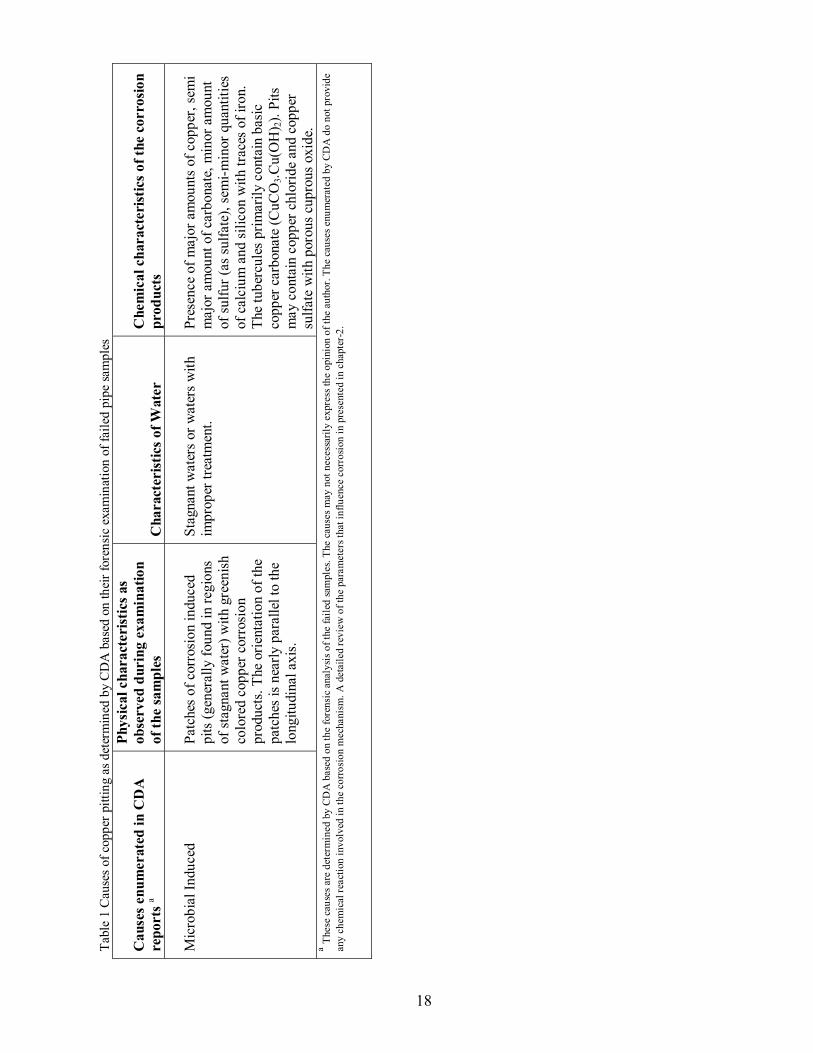
Table 1 provides a summary of various causes of failures and the associated
characteristics as identified by CDA.

Tabl
e 1
Cau
ses o
f cop
per p
ittin
g as
det
erm
ined
by
CD
A b
ased
on
thei
r for
ensi
c ex
amin
atio
n of
faile
d pi
pe sa
mpl
es
Cau
ses e
num
erat
ed in
CD
A
repo
rts a
Phys
ical
cha
ract
erist
ics a
s ob
serv
ed d
urin
g ex
amin
atio
n of
the
sam
ples
C
hara
cter
istic
s of W
ater
C
hem
ical
cha
ract
erist
ics o
f the
cor
rosio
n pr
oduc
ts
Chl
orid
e/ C
hlor
ine
indu
ced
pitti
ng. (
Poss
ible
sou
rce
sold
erin
g flu
x or
disi
nfec
tant
)
Nar
row
ban
ds o
f pits
runn
ing
long
itudi
nally
alo
ng th
e pi
pe.
Pits
are
gen
eral
ly lo
caliz
ed.
Pres
ence
of g
reen
ish
copp
er
corr
osio
n pr
oduc
ts th
at m
ay
have
bro
ken
loos
e fr
om la
rger
tu
berc
ules
.
If th
ere
is no
sold
erin
g flu
x us
ed
for t
he in
stal
latio
n, th
en th
e po
ssib
le so
urce
of c
hlor
ide/
ch
lorin
e m
ay b
e st
rong
ox
idiz
ing
chem
ical
whi
ch a
re
used
for d
isin
fect
ion
(som
e of
th
e ch
emic
als i
nclu
de so
dium
hy
poch
lorit
e, c
alci
um
hypo
chlo
rite
and
chlo
rinat
ed
cyan
urat
es).
If th
e co
rros
ion
is in
duce
d du
e to
sold
erin
g flu
x th
en it
may
be
due
to
amm
oniu
m c
hlor
ide,
zin
c ch
lorid
e, ti
n ch
lorid
e an
d/ o
r hy
droc
hlor
ic a
cid
that
are
ty
pica
lly p
rese
nt in
the
flux.
Pres
ence
of r
eddi
sh b
row
n co
pper
oxi
de
alon
g w
ith m
ajor
am
ount
s of c
oppe
r, ox
ygen
and
chl
orid
e, m
inor
qua
ntiti
es o
f sil
icon
, alu
min
um a
nd c
alci
um a
nd se
mi-
min
or a
mou
nts o
f iro
n, su
lfur a
nd
pota
ssiu
m. P
rese
nce
of c
hlor
ides
in m
ajor
qu
antit
ies,
typi
cally
the
gree
nish
col
ored
pr
oduc
ts c
onta
in c
oppe
r chl
orid
e w
hich
m
ay c
oexi
st w
ith p
orou
s cup
rous
oxi
de.
The
tube
rcul
es c
onta
in p
rimar
ily b
asic
co
pper
car
bona
te (C
uCO
3.Cu(
OH
) 2)
Pitti
ng o
ccur
red
by o
xyge
n-di
ffer
entia
l -ty
pe, c
once
ntra
tion-
cell
corr
osio
n.
Dep
ositi
on o
f sili
ca in
pre
senc
e of
alu
min
um, I
ron
or su
lfate
. Pr
esen
ce o
f tub
ercu
les
of
gree
nish
col
or c
oppe
r cor
rosi
on
prod
ucts
.
Alu
min
um o
r Iro
n >
0.1
mg/
L w
ith a
ppre
ciab
le a
mou
nts o
f sil
ica
and
pres
ence
of d
issol
ved
oxyg
en.
Pres
ence
of m
ajor
am
ount
s of c
oppe
r, iro
n,
silic
a an
d ox
ygen
alo
ng w
ith le
sser
am
ount
s of a
lum
inum
, sem
i maj
or a
mou
nt
of c
alci
um a
nd s
emi m
inor
am
ount
s of
phos
phor
ous a
nd su
lfur.
The
tube
rcul
es
prim
arily
of b
asic
cop
per c
arbo
nate
(C
uCO
3.Cu(
OH
) 2) o
r bas
ic c
oppe
r sul
fate
(C
uSO
4.3C
u(O
H) 2)
or b
oth.
Sig
nific
ant
amou
nt o
f cop
per o
xide
(Cu 2
O) w
ith le
sser
qu
antit
ies
of c
hlor
ide
and
phos
phor
us.
Dep
osits
may
incl
ude
hem
atite
(Fe 2
O3),
and
sil
ica
diox
ide
(SiO
2).
15

Tabl
e 1
Cau
ses o
f cop
per p
ittin
g as
det
erm
ined
by
CD
A b
ased
on
thei
r for
ensi
c ex
amin
atio
n of
faile
d pi
pe sa
mpl
es
Cau
ses e
num
erat
ed in
CD
A
repo
rts a
Phys
ical
cha
ract
erist
ics a
s ob
serv
ed d
urin
g ex
amin
atio
n of
the
sam
ples
C
hara
cter
istic
s of W
ater
C
hem
ical
cha
ract
erist
ics o
f the
cor
rosio
n pr
oduc
ts
Hea
ting
of w
ater
con
tain
ing
appr
ecia
ble
amou
nt o
f iro
n,
Alu
min
um o
r Sili
con
Pres
ence
of L
ocal
ized
pitt
ing
with
por
ous r
eddi
sh b
row
n cu
prou
s oxi
de o
verla
id w
ith
gree
nish
col
ored
cor
rosi
on
prod
ucts
.
Wat
er w
ith a
ppre
ciab
le a
mou
nt
of ir
on o
r iro
n ox
ides
OR
Wat
er
with
sign
ifica
nt a
mou
nt o
f sili
ca
(as S
iO2)
OR
Wat
er w
ith
alum
inum
> 0
.1 m
g/L
Pres
ence
of m
ajor
am
ount
s of c
oppe
r, ox
ygen
and
car
bona
tes,
min
or a
mou
nts o
f su
lfur (
as su
lfate
), se
mi m
inor
am
ount
s of
alum
inum
and
silic
on. T
he g
reen
ish
colo
red
prod
ucts
prim
arily
con
sist
of b
asic
cop
per
carb
onat
e (C
uCO
3.Cu(
OH
) 2) w
hich
may
be
adm
ixed
with
som
e de
posi
ts o
f cup
rous
ox
ide.
Pre
senc
e of
cup
ric o
xide
(CuO
) is
com
mon
whe
re th
e te
mpe
ratu
re e
xcee
d 16
0 F
Failu
re in
itiat
ed fr
om o
uter
side
of
the
pipe
(Pos
sible
reas
ons
incl
ude
soil
corr
osio
n,
mec
hani
cal c
rack
etc
)
The
depo
sits
may
hav
e va
ried
phys
ical
des
crip
tion
depe
ndin
g on
the
soil
com
posi
tion.
Pr
esen
ce o
f lon
gitu
dina
l or
circ
umfe
rent
ial c
rack
s in
case
of
stre
ss c
orro
sion.
Gen
eral
ly th
e st
ress
cra
cks a
re
asso
ciat
ed w
ith h
igh
pres
sure
80
psi (
gage
)
Gre
enish
col
ored
pro
duct
s prim
arily
co
nsist
ing
copp
er c
hlor
ide.
The
cor
rosi
on
prod
ucts
may
incl
ude
maj
or a
mou
nts o
f co
pper
, oxy
gen
and
chlo
ride
and
less
er
amou
nt o
f Alu
min
um, s
ilico
n,
phos
phor
ous,
pota
ssiu
m, c
arbo
n an
d iro
n de
pend
ing
upon
the
soil
com
posi
tion.
Er
osio
n/ c
orro
sion
due
to h
ighe
r ve
loci
ties o
r Loc
aliz
ed tu
rbul
ent
flow
U-s
hape
d pi
ts a
nd u
nder
cut
ting
wav
elet
form
atio
n. S
igni
fican
t re
duct
ion
in tu
be w
all,
abse
nce
of a
ny c
orro
sion
prod
ucts
at t
he
loca
tion
of p
inho
le.
Soft
wat
er o
r wat
er w
ith z
ero
hard
ness
and
esp
ecia
lly
cont
aini
ng d
issol
ved
oxyg
en o
r ca
rbon
dio
xide
. Or w
ater
gre
ater
th
an 8
0 ps
i (ga
ge) a
nd v
eloc
ities
gr
eate
r tha
n 4
to 5
feet
per
se
cond
. For
hot
wat
er, a
te
mpe
ratu
re g
reat
er th
an 1
60 F
.
Cup
ric o
xide
(CuO
) may
be
pres
ent i
n ho
t w
ater
pip
es w
here
tem
pera
ture
exc
eeds
160
F
No
corr
osio
n or
no
reas
on
esta
blish
ed.
One
or m
ore
cond
ition
s fro
m a
ll th
e re
ason
s cite
d ab
ove
that
may
be
sim
ulta
neou
sly
occu
rrin
g to
geth
er.
16

Tabl
e 1
Cau
ses o
f cop
per p
ittin
g as
det
erm
ined
by
CD
A b
ased
on
thei
r for
ensi
c ex
amin
atio
n of
faile
d pi
pe sa
mpl
es
Cau
ses e
num
erat
ed in
CD
A
repo
rts a
Phys
ical
cha
ract
erist
ics a
s ob
serv
ed d
urin
g ex
amin
atio
n of
the
sam
ples
C
hara
cter
istic
s of W
ater
C
hem
ical
cha
ract
erist
ics o
f the
cor
rosio
n pr
oduc
ts
Poor
wor
kman
ship
. Jo
inin
g tu
bes
not s
quar
ely
cut
and
ream
ed p
rope
rly p
rior t
o so
lder
ing.
Glo
bule
of s
olde
r may
be
pre
sent
. Lea
k m
ay in
itiat
e at
jo
ints
or m
ay b
e tri
gger
ed ju
st
dow
nstre
am o
f the
sold
er jo
int
that
is im
prop
erly
cut
fini
shed
NA
Th
e lo
osel
y fr
iabl
e gr
eeni
sh m
ater
ial
cont
ains
pro
duct
s hav
ing
carb
onat
e.
Sulfi
de in
duce
d pi
tting
. Pr
esen
ce o
f loc
aliz
ed p
its
cove
red
with
rela
tivel
y la
rger
tu
berc
ules
of f
riabl
e co
pper
co
rros
ion
prod
ucts
. The
size
of
the
tube
rcul
e pr
opor
tiona
l to
the
dept
h of
the
perf
orat
ion.
Sulfi
de >
0.0
2 m
g/L
Pres
ence
of m
ajor
am
ount
s of C
oppe
r and
ox
ygen
, sem
i maj
or q
uant
ities
of s
ilico
n an
d m
inor
am
ount
s of s
ulfu
r, ca
rbon
ate
and
phos
phor
ous.
Pres
ence
of c
oppe
r car
bona
te
(CuC
O3.C
u(O
H) 2)
and
cop
per s
ulfa
te, s
ome
of w
hich
in th
e fo
rm o
f bro
chan
tite
(CuS
O4.3
Cu(
OH
) 2).
Agg
ress
ive
wat
er
Pres
ence
of v
olum
inou
s tu
berc
ules
of g
reen
col
ored
co
pper
cor
rosi
on p
rodu
cts.
The
corr
osio
n in
duce
d pi
ts u
nder
the
tube
rcul
es c
onta
in re
ddis
h br
own
cupr
ous o
xide
(Cu 2
O).
Car
bon
diox
ide
exce
edin
g 25
m
g/ L
and
app
reci
able
su
spen
ded
solid
s in
form
of
silic
a.
Maj
or a
mou
nts o
f cop
per,
silic
on a
nd
oxyg
en, w
ith s
emi m
ajor
am
ount
s of
carb
onat
es a
nd se
mi-
min
or to
min
or
quan
titie
s of
iron
, mag
nesi
um, a
lum
inum
, m
anga
nese
and
cal
cium
. The
tube
rcul
es
prim
arily
con
tain
bas
ic c
oppe
r car
bona
te
(CuC
O3.C
u(O
H) 2)
that
may
be
mix
ed w
ith
varie
ty o
f pro
duct
s lik
e hy
drat
ed h
emat
ite,
silic
a an
d ca
lciu
m c
arbo
nate
.
17
Tabl
e 1
Cau
ses o
f cop
per p
ittin
g as
det
erm
ined
by
CD
A b
ased
on
thei
r for
ensi
c ex
amin
atio
n of
faile
d pi
pe sa
mpl
es
Cau
ses e
num
erat
ed in
CD
A
repo
rts a
Phys
ical
cha
ract
erist
ics a
s ob
serv
ed d
urin
g ex
amin
atio
n of
the
sam
ples
C
hara
cter
istic
s of W
ater
C
hem
ical
cha
ract
erist
ics o
f the
cor
rosio
n pr
oduc
ts
Mic
robi
al In
duce
d Pa
tche
s of c
orro
sion
indu
ced
pits
(gen
eral
ly fo
und
in re
gion
s of
stag
nant
wat
er) w
ith g
reen
ish
colo
red
copp
er c
orro
sion
pr
oduc
ts. T
he o
rient
atio
n of
the
patc
hes i
s nea
rly p
aral
lel t
o th
e lo
ngitu
dina
l axi
s.
Stag
nant
wat
ers o
r wat
ers w
ith
impr
oper
trea
tmen
t.
Pres
ence
of m
ajor
am
ount
s of c
oppe
r, se
mi
maj
or a
mou
nt o
f car
bona
te, m
inor
am
ount
of
sulfu
r (as
sulfa
te),
sem
i-min
or q
uant
ities
of
cal
cium
and
silic
on w
ith tr
aces
of i
ron.
Th
e tu
berc
ules
prim
arily
con
tain
bas
ic
copp
er c
arbo
nate
(CuC
O3.C
u(O
H) 2)
. Pits
m
ay c
onta
in c
oppe
r chl
orid
e an
d co
pper
su
lfate
with
por
ous c
upro
us o
xide
. a T
hese
cau
ses a
re d
eter
min
ed b
y C
DA
bas
ed o
n th
e fo
rens
ic a
naly
sis o
f the
faile
d sa
mpl
es. T
he c
ause
s may
not
nec
essa
rily
expr
ess t
he o
pini
on o
f the
aut
hor.
The
caus
es e
num
erat
ed b
y C
DA
do
not p
rovi
de
any
chem
ical
reac
tion
invo
lved
in th
e co
rros
ion
mec
hani
sm. A
det
aile
d re
view
of t
he p
aram
eter
s tha
t inf
luen
ce c
orro
sion
in p
rese
nted
in c
hapt
er-2
.
18

19
Distribution of pinhole leak failures based on CDA reports (1975~ 2004) Distribution of pinhole leak failures by various pipe functions
Most of the pipe failures were in cold water pipes with about forty-two percent,
seventeen percent of the leaks were in hot water pipes, and sixteen percent failures were in
hydronic system which circulates hotwater continuously. It is pointed out that this constant
circulation results in turbulence and possible high velocities leading to erosion corrosion. The
distribution of the failure reports based on the pipe category is presented in Figure 2. The details
of the annual breakup for each category of pipe are presented in Table A-1.1 (Appendix A-1).
Service Lines7.96%
Others/ Not known14.11%
Cold Water42.04%
Hot Water17.15%
Hydronic15.85%
Fire Supression2.89%
Figure 2 Average percent failures by pipe categories

20
Distribution of pinhole leak failures by various failure mechanisms
Figure 3 shows the averaged percent distribution of causes of failures. Chloride induced
pitting constituted thirty percent of the leaks; seventeen percent erosion corrosion; thirteen
percent due to external corrosion or mechanical damage; eleven percent due to oxygen-
differential type - concentration cell corrosion; ten percent due to aggressive water; eight percent
due to excessive heating of water that contains iron or salts of iron; and eleven percent due to
poor workmanship, sulfide and microbial corrosion. In most cases where the chloride induced
pitting has taken place, soldering flux or improper soldering are identified as the sources of
chloride. Other identified sources of chloride include chlorine or other oxidizing agents used for
disinfection these include sodium hypochlorite, calcium hypochlorite and chlorinated cyanurates.
Chloride/ Chlorine, 29.86%
Erosion-Corrosion, 17.06%
Failure initiated outside, 13.10%
Oxygen-Differential, 10.97%
Excessive heating of w ater, 8.38%
Aggressive Water, 9.75%
All other (Sulfide, Poor Workmanship, Microbial
and other or No leak reported), 10.89%
Figure 3 Average percent distribution causes of failures for all categories of pipe

21
The temporal patterns based on the failure causal mechanisms over a 30 year period (1975 ~
2004) are presented in Figures A-1.1 through A-1.10 (Appendix A-1). Chloride induced pitting,
Oxygen differential type pitting and pitting due to Excessive heating of water show an increasing
trend, while failures due to Erosion corrosion and Aggressive water show a decreasing trend over
a thirty year period. Other causes do not show either increasing or decreasing trend over the
stated period. The annual break down for the failure causal mechanisms is presented in Table A-
1.2 (Appendix A-1). The failure causes are further segregated based on the pipe category (cold
water, hot water, and unknown). The cold water category consists of failure reports from cold
water pipes, service laterals and fire suppression system. The hot water category consists of
failure reports from hot water pipes and hot water recirculation system. The others/ unknown
category consists of failure reports for which the pipe category is not defined in the CDA reports.
Cold water category
A total of 731 reports fall into this category. Figure 4 shows the averaged percent
distribution of causes of failure. On an average, chloride/ chlorine induced pitting constituted
forty-three percent of the failures; aggressive water fifteen percent; oxygen-differential twelve
percent; external failures twelve percent; and eighteen percent due to erosion-corrosion, poor
workmanship, sulfide, microbiological and no leak or no corrosion. The temporal patterns of
failure mechanisms for cold water category are presented in Figure A-1.11 through A-1.15
(Appendix A-1). The annual breakup of the failure mechanisms for this category is presented in
Table A-1.3 (Appendix A-1).

22
Other (include Erosion-Corrosion, Poor
w orkmaship, Sulfide and No corrosion/ No leak/ Other, 17.92%
Aggressive Water, 14.64%
Failure initiated from outside, 12.31%
Oxygen-Differential, 12.45%
Chloride/ Chlorine, 42.68%
Figure 4 Average percent distribution causes of failures for cold water category
Hot water category
A total of 456 reports fall into this category. The averaged percent breakup of the failure
causes for this category is shown in Figure 5. On an average, erosion-corrosion constitutes thirty-
four percent of the failures; excessive heating of water twenty three percent; chloride eleven
percent; external failures eleven percent; and twenty one percent constitutes oxygen differential
type, aggressive water, poor workmanship, sulfide, microbiological and no corrosion/ no cause
established. The temporal patterns of failure mechanisms for hot water category are presented in
Figures A-1.16 through A-1.20 (Appendix A-1). The annual breakup of failure mechanism for
this category is presented in Table A-1.4 (Appendix A-1).

23
Erosion-Corrosion, 33.99%
Excessive Heating of w ater, 23.03%Chloride/ Chlorine,
11.18%
Failure initiated from outside, 10.53%
All Others (includes Oxygen-Dif ferential, Poor w orkmanship, Sulfide, Microbial
induced, No corrosion/ No leak / other,
21.27%
Figure 5 Average percent distribution causes of failures for hot water category
Other or unknown pipe category
A total of 195 reports fall into this category. The averaged percent breakup of the failure
causes for this category is shown in Figure 6. On an average, externally initiated failure
constitutes twenty percent of this category; chloride nineteen percent; no corrosion/ no cause
established fifteen percent; erosion corrosion thirteen percent; and thirty one percent includes,
oxygen-differential type, sulfide induced, aggressive water, poor workmanship and excessive
heating of water. The annual breakup of failure mechanism for this category is presented in
Table A-1.5 (Appendix A-1).

24
Chloride/ Chlorine, 19.49%
Others (Include Oxygen Differential, Sulf ide,
Aggressive w ater, Poor w orkmanship,
Excessive Heating of w ater), 31.28%
Erosion-Corrosion, 13.33%
No Corrosion/ No leak/ Other, 15.38%
Failure initiated outside, 20.51%
Figure 6 Average percent distribution causes of failures for other/ unknown category
Distribution of pinhole leak failures by pipe characteristics
The analysis results for 476 reports from 1998~ 2004, are presented in Tables B-1.1
through B-1.3 (Appendix B-1).
Leak types
On an average, seventy-one percent of the reports were for pinhole type pipe failures,
twenty-nine percent reports contained information about other types of failures. The annual
breakup for both these categories of failures is presented in Table B-1.1 (Appendix B-1).
Pipe type
Most of the leaks occurred in the M and L type of copper pipes with, forty-four percent
for L-type, and forty-three percent for M-type, nine percent for K-type, and three percent were

25
left unclassified. The lesser number of leak incidents in K type pipe is understood as K type
pipes have more thickness as compared to M and L type pipes. The annual breakup for each
category of pipes is presented in Table B-1.2 (Appendix B-1).
Pipe Orientation
Most of the reported failures were in the horizontal pipes, on an average, forty-four
percent of the reported failures were in horizontal pipes, ten percent were in vertical pipes and
forty six percent reports did not contain information about the leak location. The annual breakup
for the leak location is included in Table B-1.2 (Appendix B-1).
Pipe size
Majority of failure reports were constituted by half inch (0.5 in) and three quarter inch
(0.75 in) pipe sizes, with thirty-seven percent of the failure reports are for half an inch pipe, and
thirty-nine percent for three quarter inch pipe, and ten percent for one inch pipe and fourteen
percent are for non-plumbing systems including refrigerant systems, heat pumps, and service
laterals. The annual breakup of failure reports for different pipe sizes in shown in Table B-1.3
(Appendix B-1).
Source of water
Most of the reported failures are from dwelling units that are having a well water supply
with forty-six percent of failures, nineteen percent for Surface/ River/ Lake water supply and
thirty-five percent with unknown supply source. The annual breakup of various sources of water
supply is included in Table B-1.3 (Appendix B-1).
26
Comments on CDA analysis
To summarize the temporal trends of the failure mechanisms suggest a significant
decrease in the failures due to aggressive water. Aggressive water is a generic term used by
CDA, some of the definitions of aggressive water from CDA reports include, water with higher
(> 25 mg/L) carbon dioxide concentration, and / or with high sulfate to bicarbonate ratio and / or
high sulfate to chloride ratio. The role of carbon dioxide in copper corrosion is not clearly
defined in literature. Some of the failure causes enumerated by CDA do not define a supporting
mechanism based on water chemistry; hence a firm opinion on the exact cause of failure cannot
be formed. Most often when chloride was cited as the cause of the failure, the source of chloride
was identified as the soldering flux or disinfectants, although the CDA reports do not explain the
possible reaction or kinetics that could have been involved in such a reaction. Importantly, the
role of chloride ion is questionable with respect to the present understanding of copper pitting, on
many instances chloride is identified as a species that initiates pitting (Warraky et al. 2004) while
some scientists have reported that chloride inhibits pitting in long term (Edwards et al. 1994).
The failure causes were identified based on the failed specimen; however the pipes that did not
fail in the same home were not tested for an objective comparison. Hence, any firm conclusion
on the causes of failure cannot be made based on the CDA findings. A detailed review of the
physical and chemical parameters that influence pitting is provided in chapter-2.
Analysis of the CDA database suggests that majority of the failures are in horizontal cold
water pipes that are ½” and ¾” type M or L copper tubes. The data shows majority of failures for
homes that have ground water supply.

27
Spatial patterns of pinhole leaks
Methodology
The spatial distribution of the pinhole leaks is studied using the CDA data base and the
Expert Opinion survey. The results of the analysis from the CDA data base and the Expert
opinion survey were verified by the Plumber Survey-I. For the present analysis, spatial
information about pinhole leak occurrence is obtained from Expert Opinion Survey and CDA
database. Since, the analysis of CDA database was done progressively with time, five years
(2000~ 2004) of CDA data is used for this analysis. The objectives behind studying the spatial
patterns are to identify hotspots as well as areas that are relatively free of pinhole leak incidents.
A weighted count system is used to obtain a preliminary classification on a city and state level.
The preliminary classification is then tested for pinhole leak incidents for the areas that do not
surface in the preliminary analysis.
The weighted count is assigned by assessing the information parameters provided by that
particular database/ survey. Some of the crucial information parameter used for assigning the
weighted count are, information related to the location (address), type of dwelling unit, water
quality parameters, pipe size, hot or cold water pipe, horizontal or vertical pipe, type of copper
pipe (K, L or M), time of installation and time of first leak, any hydraulic parameter (pressure
and velocity). Each year of CDA database was treated as a single data set. Since, the CDA
reports contain most of the information parameters that identifies each pinhole failure in spatial
and temporal terms hence every failure report from CDA database was assigned a weight of “1”.
For example year 1999 and year 2000 are treated as two different data sets. Also, if a city
appears more than once in a particular year, it is counted that many times because each data point

28
in CDA corresponds to a different dwelling unit. The Expert Opinion Survey, provided names of
the affected communities and states where pinhole leak were reported at least once. Moreover,
the survey does not provide specific information parameters that could identify every leak in
terms of spatial and temporal coordinates. There was also a chance of multiple references could
have been made for a single incident. Hence, a weight of “1” is assigned to any city or state
irrespective of the number of times it appears in the survey results.
Results and Discussions
The weighted count analysis was performed for city and state, separately. The top five
states with maximum number of counts are California, Maryland, Ohio, Florida and
Pennsylvania. Interestingly, five states, namely, Delaware, Louisiana, Mississippi, North Dakota,
and New Hampshire do not appear in the preliminary classification. Amongst, the top fifteen
heavily populated cities, four cities are absent in the preliminary classification, these cities are
Austin (TX), Columbus (OH), Detroit (MI) and Memphis (TN).
Plumber Survey-I
As a verification of the preliminary classification, a telephone survey was conducted by
calling plumbers in the nine locations. The description of the Plumber Survey-I is presented in
the following section. As mentioned earlier, five states were not referenced in the previous CDA
reports namely or from any of the previous expert or initial surveys: Louisiana, Delaware,
Mississippi, New Hampshire, and North Dakota. A survey was conducted to confirm whether
copper pitting is occurring in these states. Plumbers in the major city of each state were

29
interviewed via telephone. In addition, four of the top fifteen heavily populated cities namely,
Austin (TX), Columbus (OH), Detroit (MI) and Memphis (TN) were also included in this survey.
Survey Method
The names, addresses and telephone numbers of the plumbers were selected, randomly
from telephone directory yellow pages. The survey was conducted from July 7th 2005 through
August 8th 2005. Due to difficulties in contacting plumbers on the phone, the survey was
conducted at different times of the day. Despite spreading the call- schedule, the success rate for
the survey was fairly low as shown in Table 2. Most calls ended up with no response. The
successful calls, that did reach the plumbers, were rather short due to their busy schedules.
Because of these reasons, all the questions listed in Table 3 could not be asked to a single
plumber, instead the questions were asked in decreasing order of priority. First priority was
given to the set of questions that relate to the extent of the pinhole leaks in that particular area.
These included questions on the possible causes of the pinhole leaks. Second priority was given
to the questions related to the cost of repair, cost of re- plumbing, and questions related to the
process of repair and pipe materials.
Survey Results
A total of two hundred forty-two calls were attempted, and fifty-five calls were
successful (22% success rate). Out of fifty-five plumbers surveyed, twenty-two responded with
a definite yes about the existence of the pinhole leaks, twenty-five stated that it is not a common
problem, and eight stated that the problem does not exist. The city-wise results from the survey

30
about the extent of pinhole leaks are tabulated in Table 2. There were several factors enumerated
by the plumbers that could lead to pinhole leaks (Table 4).
All of the plumbers stated that they do the repairs on an hourly basis, with the material
cost added to the labor cost. They also stated that fixing the dry wall is not a part of the plumbing
job and the homeowner has to engage a separate general contractor for drywall fixing and
finishing. The labor rate for repair jobs varied from city to city, generally the labor rate for the
repairs varies between $ 45 and $ 75 (Table 5). Data regarding the cost of a complete re-
plumbing was obtained for only two of the cities. The cost of re-plumbing for a two bath, two
story house in Austin (TX) varied between $ 2500 ~ $ 3500, while in Columbus (OH) the cost of
re plumb varied between $ 3000 ~ $ 4000. Most of the plumbers in other cities either refused to
give prices on phone or they expressed their inability to answer questions related to costs.
Comments on Plumber-I survey
Although, these cities/ states were not referenced by any of the sources used for
preliminary spatial classification, but the survey results have verified the occurrence of pinhole
leaks by at least one plumber in all these areas except Detroit. However, in an earlier survey of
plumbers by Dr Marc Edwards, the plumbers in Detroit had reported pinhole leaks. Hence, the
discrepancy in the present results may be due to small sample of plumbers considered during the
survey. Among the causes enumerated by the plumbers, the most cited reasons include the age of
the plumbing, intrusions in pipe, well water and soldering flux. Interestingly, the first three
causes (namely, Age of the pipe, Intrusions or weak spots inside pipes and well water) have
never been cited in the CDA database.

31
Based on the plumber survey, it is established that even the locations that are not cited by
the Experts and the CDA database, have been confirmed for pinhole incident by at least one
plumber. Interestingly, there is no leak incident reported from Delaware in the entire 38 years
period (1966~ 2004), however, 7 out of 9 plumbers in Wilmington confirmed the pinhole leak
incidents in the city. Hence, it is concluded that the pinhole leak is a wide spread problem and
even with the best available resources the spread of pinhole leak could not be ascertained.
The spatial patterns based on the CDA reports are shown in Figure 1, in the beginning of
the chapter. Additional data for 1998 and 1999 was added to create Figure 1. Certain hot spots
emerge very clearly from Figure 1, these include communities in Ohio and Florida and certain
parts of California. Although, the data used for the creation of Figure 1 is not complete
representative of the spatial spread of pinhole leaks, but even with the limited data, the spread of
the pinhole leak is evident on a nationwide scale.

32
Table 2 City wise results from Plumber’s Survey about the extent of pinhole leaks
# of response on Pinhole Leaks
S.no City State
Total # of calls made
Total # of successful calls Yes
Not a common problem No
1 Austin TX 30 4 1 3 02 Columbus OH 23 6 2 4 03 Detroit MI 25 6 0 1 54 Memphis TN 35 4 1 2 15 New Orleans LA 36 6 1 4 16 Wilmington DE 24 9 7 2 07 Jackson MS 33 5 1 4 08 Manchester NH 17 7 6 1 09 Bismarck ND 19 8 2 5 1
Table 3 List of questions for the Plumber Survey Questions Remarks
Do you have pinhole leaks in copper plumbing in your area? Priority-1
How often do you get complaints of pinhole leaks? Is it a common problem? Priority-1
By your experience what are the factors that cause pinhole leaks? Priority-1
How much does it costs to repair a pinhole leak? Priority-2
What is the cost of re plumbing a 2 BR, two storey house with 2 bathrooms? Priority-2
Is the dry wall removal & fixing cost included in the above costs? Priority-2
Do you remove the old pipes or leave them in place when you re plumb a house? Priority-2
By your experience which pipe material works out best for the home plumbing
system?
Priority-2
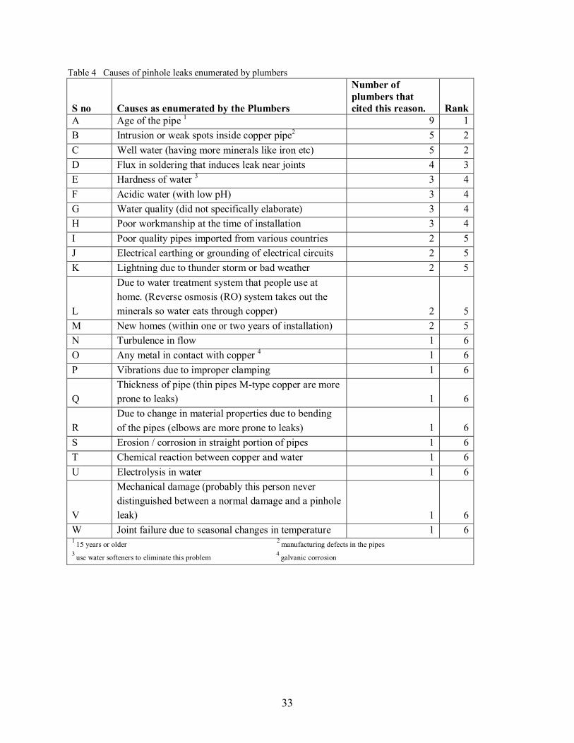
33
Table 4 Causes of pinhole leaks enumerated by plumbers
S no Causes as enumerated by the Plumbers
Number of plumbers that cited this reason. Rank
A Age of the pipe 1 9 1B Intrusion or weak spots inside copper pipe2 5 2C Well water (having more minerals like iron etc) 5 2D Flux in soldering that induces leak near joints 4 3E Hardness of water 3 3 4F Acidic water (with low pH) 3 4G Water quality (did not specifically elaborate) 3 4H Poor workmanship at the time of installation 3 4I Poor quality pipes imported from various countries 2 5J Electrical earthing or grounding of electrical circuits 2 5K Lightning due to thunder storm or bad weather 2 5
L
Due to water treatment system that people use at home. (Reverse osmosis (RO) system takes out the minerals so water eats through copper) 2 5
M New homes (within one or two years of installation) 2 5N Turbulence in flow 1 6O Any metal in contact with copper 4 1 6P Vibrations due to improper clamping 1 6
Q Thickness of pipe (thin pipes M-type copper are more prone to leaks) 1 6
R Due to change in material properties due to bending of the pipes (elbows are more prone to leaks) 1 6
S Erosion / corrosion in straight portion of pipes 1 6T Chemical reaction between copper and water 1 6U Electrolysis in water 1 6
V
Mechanical damage (probably this person never distinguished between a normal damage and a pinhole leak) 1 6
W Joint failure due to seasonal changes in temperature 1 61 15 years or older 2 manufacturing defects in the pipes 3 use water softeners to eliminate this problem 4 galvanic corrosion
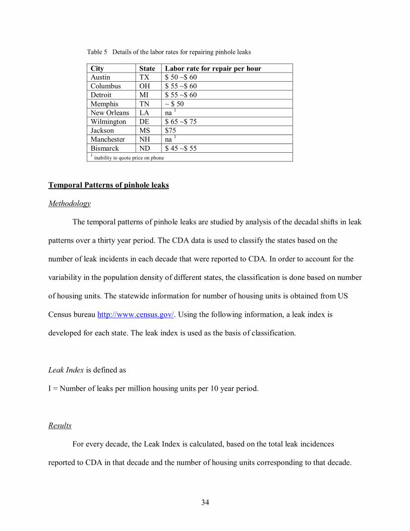
34
Table 5 Details of the labor rates for repairing pinhole leaks
City State Labor rate for repair per hour Austin TX $ 50 ~$ 60 Columbus OH $ 55 ~$ 60 Detroit MI $ 55 ~$ 60 Memphis TN ~ $ 50 New Orleans LA na 1 Wilmington DE $ 65 ~$ 75 Jackson MS $75 Manchester NH na 1 Bismarck ND $ 45 ~$ 55 1 inability to quote price on phone
Temporal Patterns of pinhole leaks
Methodology
The temporal patterns of pinhole leaks are studied by analysis of the decadal shifts in leak
patterns over a thirty year period. The CDA data is used to classify the states based on the
number of leak incidents in each decade that were reported to CDA. In order to account for the
variability in the population density of different states, the classification is done based on number
of housing units. The statewide information for number of housing units is obtained from US
Census bureau http://www.census.gov/. Using the following information, a leak index is
developed for each state. The leak index is used as the basis of classification.
Leak Index is defined as
I = Number of leaks per million housing units per 10 year period.
Results
For every decade, the Leak Index is calculated, based on the total leak incidences
reported to CDA in that decade and the number of housing units corresponding to that decade.

35
The decades are considered in reverse chronological order for the analysis. These are namely,
first decade (1995~2004), second decade (1985~1994) and third decade (1975~1984). An
increase or decrease in the “Leak Index” is considered as an indicator of the shift in trend of
pinhole leaks in that state. The classification based on the leak index for the three decades is
presented in Figure 7 through 9. The temporal shifts in leak patterns between the decades are
presented in Figure 10 and 11. The results of the analysis are presented in Table 6.
Table 6 Analysis for decadal patterns of pinhole leaks, based on CDA data (1975~2004)
Leak Index = Total Leaks per million housing units
Trend based on change in Leaks Index
States Decade 1 (1995~2004)
Decade 2 (1985~1994)
Decade 3 (1975~1984) Decade 1~2 Decade 1~3
Alaska 15.07 12.90 6.14 Increase Increase Alabama 3.47 2.39 2.73 Increase Increase Arkansas 4.16 2.00 1.11 Increase Increase Arizona 7.30 13.26 16.22 Decrease Decrease California 7.68 5.81 6.47 Increase Increase Colorado 3.11 7.45 25.12 Decrease Decrease Connecticut 15.68 1.51 1.73 Increase Increase Delaware 0.00 0.00 0.00 No change No change Florida 5.12 6.72 5.02 Decrease Increase Georgia 2.01 1.14 3.94 Increase Decrease Hawaii 6.38 28.22 2.99 Decrease Increase Iowa 3.18 1.75 6.19 Increase Decrease Idaho 1.81 4.84 10.66 Decrease Decrease Illinois 2.01 2.88 1.62 Decrease Increase Indiana 9.18 2.23 0.96 Increase Increase Kansas 5.18 2.87 2.09 Increase Increase Kentucky 3.90 0.00 0.00 Increase Increase Louisiana 0.53 0.58 1.29 Decrease Decrease Massachusetts 6.79 5.26 4.08 Increase Increase Maryland 17.30 2.11 3.82 Increase Increase Maine 1.50 0.00 1.99 Increase Decrease Michigan 1.62 1.56 0.56 Increase Increase Minnesota 5.16 3.25 3.72 Increase Increase Missouri 3.60 0.91 1.01 Increase Increase Mississippi 0.00 0.00 0.00 No change No change

36
Table 6 Analysis for decadal patterns of pinhole leaks, based on CDA data (1975~2004)
Leak Index = Total Leaks per million housing units
Trend based on change in Leaks Index
States Decade 1 (1995~2004)
Decade 2 (1985~1994)
Decade 3 (1975~1984) Decade 1~2 Decade 1~3
Montana 7.19 5.54 18.27 Increase Decrease North Carolina 1.62 0.35 0.44 Increase Increase North Dakota 0.00 18.09 15.46 Decrease Decrease Nebraska 8.12 0.00 16.00 Increase Decrease New Hampshire 0.00 0.00 7.76 No change Decrease New Jersey 4.45 5.20 5.41 Decrease Decrease New Mexico 11.18 4.75 19.69 Increase Decrease Nevada 8.87 3.85 5.88 Increase Increase New York 2.84 3.18 1.75 Decrease Increase Ohio 7.79 1.60 3.89 Increase Increase Oklahoma 3.24 0.71 3.23 Increase Increase Oregon 6.02 5.86 0.00 Increase Increase Pennsylvania 8.82 2.03 1.96 Increase Increase Rhode Island 4.51 4.82 0.00 Decrease Increase South Carolina 5.48 0.00 0.87 Increase Increase South Dakota 3.01 13.68 3.61 Decrease Decrease Tennessee 0.40 1.48 1.72 Decrease Decrease Texas 2.47 1.43 3.97 Increase Decrease Utah 9.89 8.36 67.35 Increase Decrease Virginia 5.32 2.40 1.48 Increase Increase Vermont 6.68 0.00 0.00 Increase Increase Washington 3.56 0.98 0.59 Increase Increase Wisconsin 12.15 1.95 3.22 Increase Increase West Virginia 2.35 0.00 0.00 Increase Increase Wyoming 0.00 0.00 10.63 No change Decrease District of Columbia 7.34 3.59 10.82 Increase Decrease US (Total) 5.15 3.28 4.12 Increase Increase

37
Figure 7 A three tier nationwide classification based on CDA reports (1995~2004)
Figure 8 A three tier nationwide classification based on CDA reports (1985~1994)

38
Figure 9 A three tier nationwide classification based on CDA reports (1975~1984)
Figure 10 Spatial shift of leak patterns between (1995~2004) and (1975~1984)

39
Figure 11 Spatial shift of leak patterns between (1995~2004) and (1985~1994)
Conclusions
Based on the leak index the states namely, Arizona, Colorado, Idaho, Louisiana, North
Dakota, New Jersey, South Dakota and Tennessee show a decreasing trend between first and
second decade and also between first and third decade. The states that do not show any change in
the leak index in all the three decades are Delaware and Mississippi; it is because these states do
not contain any report in the CDA database. Interestingly, the total US figures show an
increasing trend over the three decades consistently.
Maryland, California and Ohio show increasing trend, which is in agreement with the present
information on certain hotspots in these states. Interestingly, Florida shows a decreasing trend
when compared with the previous decade (1985~1994), although there have been many leak
incidents in one community in the present decade (1995~2004) and it has emerged as a hotspot

40
for pinhole leaks. Overall, considering the 30 years span of failures, copper has been a relatively
good plumbing material, except in a few hot spots that have experienced a high frequency of
failures. It has been either determined or assumed that a particular mechanism has caused or is
causing the premature copper failures. Factors that can lead to potentially aggressive copper
corrosion are discussed in the next chapter.
The present analysis shows some states with no change in leak incidents, it is primarily due to
absence of reported failures from these states. Because of this reason, the calculated leak index is
zero (Table 6). Since, the CDA reports are based on voluntary submission of failed samples, the
leak index based analysis remains inconclusive. The results should be treated as preliminary.
The actual spatial shift in patterns with time cannot be established based on CDA database alone
even though that is the well documented one.
Factors Determining Copper Pipe Selection
There are numerous factors that influence consumer’s decision in selection of a particular
pipe material. These factors encompass a spectrum of issues including durability, affordability,
resistance to corrosion, performance (taste, odor and color), safety against possible health
hazards, fire resistance, serviceability during extreme weather conditions, cost, added value to
house/ dwelling unit, willingness to pay, willingness to take risk, magnitude and type of risk,
consumers’ perception, past experience, loss of revenue (for commercial) and to some extent the
local regulations and neighborhood’s experience. For instance the use of PEX pipe is banned in
certain areas of California, although its use is approved in all the other 49 states, like wise in

41
some parts of Florida, the use of copper pipe is less preferred due to acuteness of pinhole leak
problems.
From manufacturing perspective, the characteristics that are generally desirable in the raw
materials are ductility and malleability. Since most of the metals and plastics (including modified
polymers) are intrinsically ductile and malleable, plumbing pipes are generally manufactured out
of metal, metal alloys and plastics. In general the options available to the consumer in terms of
pipe materials include Galvanized iron, Copper, Plastics (CPVC, PVC, PEX, Polybutylene) and
Stainless steel. Galvanized iron pipes are still used but their use is not very frequent especially in
residential establishments (http://www.nsf.org/consumer/plumbing/index.asp). The major
concern with galvanized iron includes build up of rust over a period of time. The rusting inside
the galvanized iron pipe may cause loss of hydraulic conductivity and may leach rust particles in
water causing red water problems.
PVC and CPVC are cost effective options however, PVC pipes tend to be more brittle and often
crack when exposed to weather; due to this CPVC is often a chosen over PVC. CPVC pipes are
corrosion resistant and can withstand high pressures, and due to their ease in installation they are
often preferred by plumbers. The concerns with CPVC pipe include microbial growth, cracking
in the event of an earthquake, plastic taste and melting in the event of fire. The solvents used for
joining these pipes may leach volatile organic compounds (VOCs). Additional concerns with
CPVC include leaching of vinyl chloride monomer (VCM), the extended exposure to VCM can
lead to neurological and liver disorders as well as cancer. The health issues related to CPVC
pipes are subjected to controversies

42
(http://www.builderswebsource.com/techbriefs/cpvccopper.htm#Benefits%20CPVC). It is
important to note that the magnitude of potential risk associated with the leaching of VCM (in
CPVC pipes) is not known hence the issues related to health concerns remain questionable.
Additionally, PVC and CPVC pipe are approved for use in United States, and these pipes comply
with NSF/ ANSI health requirements. The plastic pipes for potable water supply, bear “NSF-
PW” or “NS-61” mark, which shows that the product complies with the health requirements set
by NSF/ ANSI. (http://www.nsf.org/consumer/plumbing/index.asp). The PVC and CPVC pipes
are tested twice annually in accordance with NSF standards to ensure that the VCM level
remains below the maximum allowable limits, also the products with “NSF-PW” mark are tested
at regular interval to ensure compliance for all other properties including properties related to
health. (http://www.builderswebsource.com/techbriefs/cpvccopper.htm#Introduction).
PEX (polyethylene cross linked) pipes are flexible pipes (like electrical cables), these pipes
require different plumbing design altogether, instead of a branch and main arrangement, these
pipes require individual pipe lengths for every fixture which is connected to a common manifold.
This design increases the number of pipes and the total pipe length required for a house. But due
to lower unit price the overall cost almost equals the cost of plumbing with any other plastic
pipe. The main advantage is that each pipe is free of joints and therefore less prone to any kind of
leak. PEX pipes are also available in form for a composite pipe material, where a layer of
aluminum is sandwiched between two layers of PEX (polyethylene cross linked) material. The
use of PEX is banned in some parts of California due to potential risk of leaching MTBE (methyl
tertiary butyl ether) and benzene into drinking water, and due to its ability to spread fire rapidly.

43
(http://www.prnewswire.com/cgi-bin/stories.pl?ACCT=109&STORY=/www/story/11-18-
2004/0002464315&EDATE=). However, its use is approved in all other 49 states, and
importantly PEX pipes comply with the health requirement set by NSF/ ANSI. The plastic pipes
for potable water supply, bear “NSF-PW” or “NS-61” mark, which shows that the product
complies with the health requirements set by NSF/ ANSI.
(http://www.nsf.org/consumer/plumbing/index.asp).
Polybutylene (PB) is flexible pipe which can be easily bent, cut and easily installed at a lower
price. The material was introduced in 1970’s and has been used in about six million homes in
United States. (http://accuspec.biz/PB Plumbing.htm ). Due to leak problems associated with PB
pipes, there have been several lawsuits against the PB manufacturers. The law suit settlement
was administered by Consumer Plumbing Recovery Center (CPRC) and some of the consumers
were offered a free replacement of the entire plumbing under this settlement.
(http://www.pbpipe.com/index1.htm).
Stainless steel pipes are mainly used in industrial applications. Stainless steel provides excellent
resistance to corrosion, due to presence of chromium that forms 17~20% of stainless steel. The
stainless steel is expensive due to which its use is limited to specialized industries for conveying
chemicals or other such applications. The concern with stainless steel pipes include leaching of
chromium. However, the stainless steel pipe is approved for use in United States, and complies
with NSF/ ANSI health requirements.
(http://www.nsf.org/business/newsroom/press_release.asp?p_id=12241).

44
Copper is the most widely used material in residential and commercial plumbing. The
advantages of using copper include affordability, fire resistance, little or no health hazards, and
durability. However, due to pinhole leak incidents consumers often prefer plastic pipes over
copper. If copper pipes are used in potable waters with lower pH (< 6.5), the problems of copper
leaching may increase. The USEPA lead copper rule (1991) regulates the concentration of
copper in drinking water to a maximum contaminant limit of 1.3 mg/ L. Additional concerns
with copper pipes include metal taste especially with long stagnation periods and increased
consumption of residual disinfectant by the pipe walls.
In summary the selection of pipe material is subjective to consumers’ perception and
choice. In general, for residential establishments, cost, performance (taste, color and odor),
resistance to corrosion, affordability, durability, added value to house and health effects are
expected to be more dominant among the various factors. For commercial establishments, the
decision matrix is expected to be governed by cost and fire resistance as compared to other
parameters. The issues related to health are expected to be of lesser importance in case of
commercial establishments. Although, the selection of pipe material is highly subjective to ones’
preferences and may change from one consumer to another, hence a generic statement for the
selection criteria for either residential or commercial establishments cannot be made. Other
secondary factors which may influence consumer’s decision are consumer’s access to
information, attractive marketing strategies, special discount offers or purchase incentives and
advise from others (plumbers, consultants, architects, neighbors etc). Thus the actual decision
matrix of a consumer is complex however it is expected that the decision is likely to be
influenced by many of the factors discussed above.

45
References
1. Edwards M., Rushing J.C., Kvech S., Reiber S., Assessing copper pinhole leaks in
residential plumbing. Water Science and Technology 49 (2), 83-90.
2. Copper Development Association (CDA), Failure reports 1975~2004.
3. Washington Suburban Sanitary Commission (WSSC), pinhole leak database.
4. American Water Works Association (AWWA) and American Water Works Association
Research Foundation (AWWARF), Utility Survey- Water Stats (1996).
5. Virginia Tech Survey Research Center, Homeowner Pinhole Leak and Drinking Water
Survey (2005).
6. Bosch Darrell, Expert Opinion Survey- Virginia Tech (2004).
7. Loganathan G.V., Lee Juneseok, Farooqi Owais, Plumber Survey-I (2005).
8. Virginia Tech Survey Research Center, Plumber Survey-II (2006).
Website References
9. http://www.toolbase.org
10. http://www.plumbingsupply.com
11. http://copper.org
12. http://www.census.gov
13. http://www.nsf.org
14. http://www.builderswebsource.com
15. http://www.prnewswire.com
16. http://accuspec.biz
17. http://www.pbpipe.com

Appendix A-1
46
APPENDIX A-1
Temporal Patterns of Pinhole Leak due to various Corrosion Mechanisms
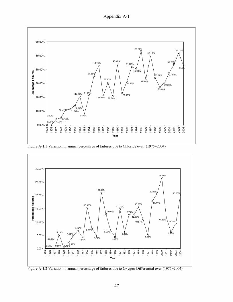
Appendix A-1
47
33.87%
27.59%
35.00%
10.71%
0.00% 4.00%
0.00%
20.45%
8.16%
11.36%
42.86%
21.05%
30.43%
20.69%
43.48%
22.95%
31.25%
41.82%
53.13%
50.00%
32.61%
5.13%
13.95%
21.15%
40.63%
43.75%
42.50%
37.68%
30.38%
52.00%
0.00%
10.00%
20.00%
30.00%
40.00%
50.00%
60.00%
1975
1976
1977
1978
1979
1980
1981
1982
1983
1984
1985
1986
1987
1988
1989
1990
1991
1992
1993
1994
1995
1996
1997
1998
1999
2000
2001
2002
2003
2004
Year
Perc
enta
ge F
ailu
res
Figure A-1.1 Variation in annual percentage of failures due to Chloride over (1975~2004)
9.33%
6.25%
11.59%
20.00%
26.58%
10.87%
5.00%
15.63%
12.73%
6.25%
14.75%
4.35%
6.90%
13.04%
21.05%
4.76%
2.27%
4.08%
6.82%
0.00%
0.00%
0.00% 0.00%
7.50%
20.69%
17.74%
5.13%
15.38%
12.50%
4.65%
0.00%
5.00%
10.00%
15.00%
20.00%
25.00%
30.00%
1975
1976
1977
1978
1979
1980
1981
1982
1983
1984
1985
1986
1987
1988
1989
1990
1991
1992
1993
1994
1995
1996
1997
1998
1999
2000
2001
2002
2003
2004
Year
Perc
enta
ge F
ailu
res
Figure A-1.2 Variation in annual percentage of failures due to Oxygen-Differential over (1975~2004)

Appendix A-1
48
25.00%
13.33%
10.00%
14.49%
11.39%
9.68%
16.09%15.00%
0.00%0.00% 0.00%
4.76%
0.00%
4.08%
0.00%
9.52%
0.00% 0.00%
3.45%
8.70%
6.56%
0.00%
7.27%
0.00%
15.00%
10.87%
0.00%
2.56%
1.92%
9.38%
0.00%
5.00%
10.00%
15.00%
20.00%
25.00%
30.00%
1975
1976
1977
1978
1979
1980
1981
1982
1983
1984
1985
1986
1987
1988
1989
1990
1991
1992
1993
1994
1995
1996
1997
1998
1999
2000
2001
2002
2003
2004
Year
Perc
enta
ge F
ailu
res
Figure A-1.3 Variation in annual percentage of failures due to Excessive heating over (1975~2004)
10.14%
10.13%
7.81%
12.50%
17.33%
26.09%
15.00%
9.38%9.09%
25.00%
9.84%
13.04%
27.59%
8.70%
10.53%
19.05%
11.36%10.20%
13.64%
9.52%
16.00%
15.79%
7.14% 7.50%
16.09%
22.58%
15.38%
6.98%
5.77% 6.25%
0.00%
5.00%
10.00%
15.00%
20.00%
25.00%
30.00%
1975
1976
1977
1978
1979
1980
1981
1982
1983
1984
1985
1986
1987
1988
1989
1990
1991
1992
1993
1994
1995
1996
1997
1998
1999
2000
2001
2002
2003
2004
Year
Perc
enta
ge F
ailu
res
Figure A-1.4 Variation in annual percentage of failures due to External failures over (1975~2004)
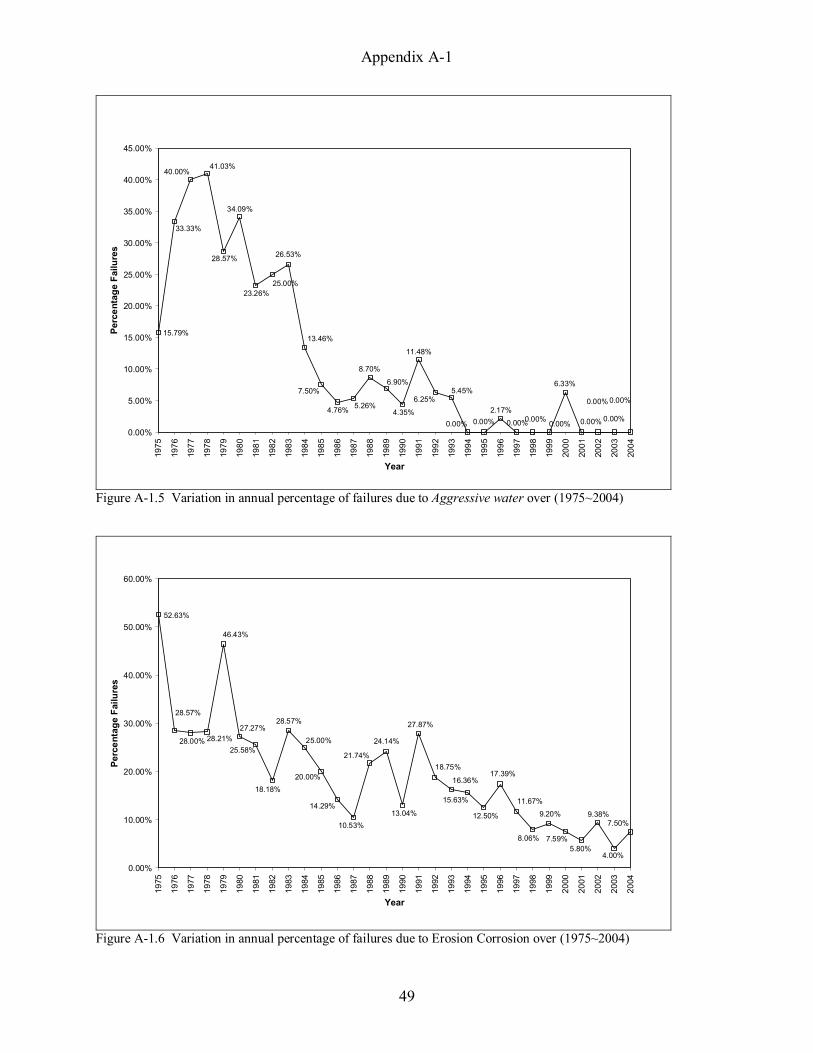
Appendix A-1
49
0.00%
0.00%
0.00%
0.00%
6.33%
13.46%
0.00% 0.00%
7.50%
28.57%
15.79%
40.00%
33.33%
25.00%
26.53%
34.09%
4.76% 5.26%
8.70%
6.90%
4.35%
11.48%
6.25%5.45%
0.00% 0.00%
2.17%
23.26%
41.03%
0.00%0.00%
5.00%
10.00%
15.00%
20.00%
25.00%
30.00%
35.00%
40.00%
45.00%19
75
1976
1977
1978
1979
1980
1981
1982
1983
1984
1985
1986
1987
1988
1989
1990
1991
1992
1993
1994
1995
1996
1997
1998
1999
2000
2001
2002
2003
2004
Year
Perc
enta
ge F
ailu
res
Figure A-1.5 Variation in annual percentage of failures due to Aggressive water over (1975~2004)
7.50%
4.00%
9.38%
5.80%7.59%
15.63%
25.00%25.58%
28.21%
8.06%
9.20%
20.00%
46.43%
52.63%
28.00%
28.57%
18.18%
28.57%27.27%
14.29%
10.53%
21.74%
24.14%
13.04%
27.87%
18.75%
16.36%
12.50%
11.67%
17.39%
0.00%
10.00%
20.00%
30.00%
40.00%
50.00%
60.00%
1975
1976
1977
1978
1979
1980
1981
1982
1983
1984
1985
1986
1987
1988
1989
1990
1991
1992
1993
1994
1995
1996
1997
1998
1999
2000
2001
2002
2003
2004
Year
Perc
enta
ge F
ailu
res
Figure A-1.6 Variation in annual percentage of failures due to Erosion Corrosion over (1975~2004)
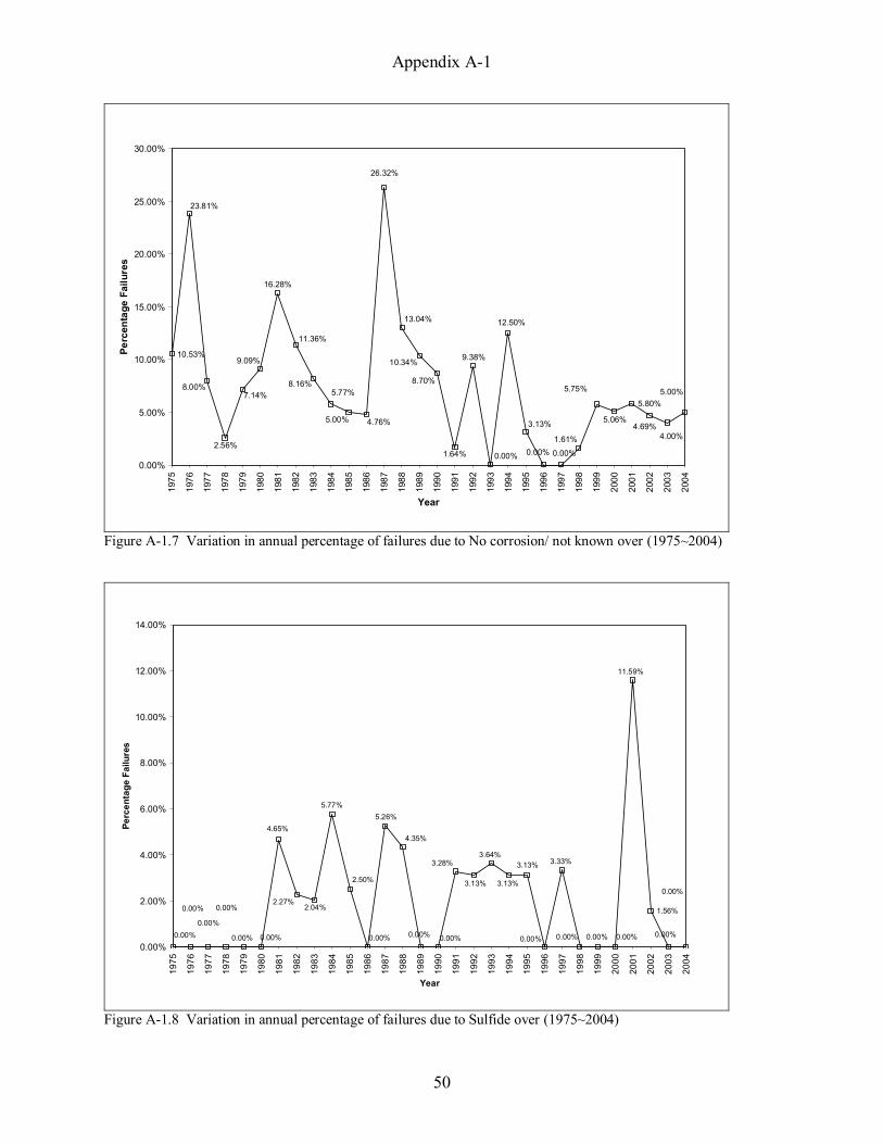
Appendix A-1
50
5.80%5.00%
4.00%4.69%
5.06%
5.77%
16.28%
2.56%1.61%
5.75%
5.00%
7.14%
10.53%
8.00%
23.81%
11.36%
8.16%
9.09%
4.76%
26.32%
13.04%
10.34%
8.70%
1.64%
9.38%
0.00%
3.13%
0.00%0.00%
12.50%
0.00%
5.00%
10.00%
15.00%
20.00%
25.00%
30.00%
1975
1976
1977
1978
1979
1980
1981
1982
1983
1984
1985
1986
1987
1988
1989
1990
1991
1992
1993
1994
1995
1996
1997
1998
1999
2000
2001
2002
2003
2004
Year
Perc
enta
ge F
ailu
res
Figure A-1.7 Variation in annual percentage of failures due to No corrosion/ not known over (1975~2004)
1.56%
3.13%
0.00%
3.33%3.13%3.64%
3.13%
3.28%
0.00%0.00%
4.35%
5.26%
0.00%0.00%
2.04%2.27%
0.00%
0.00%0.00% 0.00%
2.50%
0.00% 0.00%
0.00%
4.65%
5.77%
0.00%
11.59%
0.00%
0.00%
0.00%
2.00%
4.00%
6.00%
8.00%
10.00%
12.00%
14.00%
1975
1976
1977
1978
1979
1980
1981
1982
1983
1984
1985
1986
1987
1988
1989
1990
1991
1992
1993
1994
1995
1996
1997
1998
1999
2000
2001
2002
2003
2004
Year
Perc
enta
ge F
ailu
res
Figure A-1.8 Variation in annual percentage of failures due to Sulfide over (1975~2004)

Appendix A-1
51
0.00%
0.00%
0.00%
0.00%
1.27%
0.00%
0.00%
3.13%
0.00%0.00%
1.64%
4.35%
0.00%0.00%
0.00%
0.00%0.00%
0.00%
0.00%
0.00%
0.00%0.00%
0.00%0.00%
0.00%
0.00%
0.00%0.00%0.00%
0.00%
0.00%
0.50%
1.00%
1.50%
2.00%
2.50%
3.00%
3.50%
4.00%
4.50%
5.00%19
75
1976
1977
1978
1979
1980
1981
1982
1983
1984
1985
1986
1987
1988
1989
1990
1991
1992
1993
1994
1995
1996
1997
1998
1999
2000
2001
2002
2003
2004
Year
Perc
enta
ge F
ailu
res
Figure A-1.9 Variation in annual percentage of failures due to Microbiological over (1975~2004)
5.77%
0.00%
4.65%
0.00%
6.45%
4.60%
0.00%0.00%
5.26%
4.00%
0.00%
2.27%
8.16%
4.55%
0.00%
0.00%
0.00%
0.00%
0.00%
0.00% 0.00%
3.64%
0.00%
0.00%0.00%
1.27%
2.90%
1.56%
2.50%
0.00%0.00%
1.00%
2.00%
3.00%
4.00%
5.00%
6.00%
7.00%
8.00%
9.00%
1975
1976
1977
1978
1979
1980
1981
1982
1983
1984
1985
1986
1987
1988
1989
1990
1991
1992
1993
1994
1995
1996
1997
1998
1999
2000
2001
2002
2003
2004
Year
Perc
enta
ge F
ailu
res
Figure A-1.10 Variation in annual percentage of failures due to Poor workmanship over (1975~2004)

Appendix A-1
52
64.00%
56.52%
58.54%
54.76%
33.33%
4.17%
61.11%
34.38%
14.29%
41.67%
36.36%
63.16%
6.67%0.00% 0.00%
0.00%
33.33%
7.69%
19.05%
50.00%
42.86%
44.44%
36.36%
63.64%
40.00%
80.00%
55.17%
63.64%
73.68%
61.90%
0.00%
10.00%
20.00%
30.00%
40.00%
50.00%
60.00%
70.00%
80.00%
90.00%19
75
1976
1977
1978
1979
1980
1981
1982
1983
1984
1985
1986
1987
1988
1989
1990
1991
1992
1993
1994
1995
1996
1997
1998
1999
2000
2001
2002
2003
2004
Year
Perc
enta
ge F
ailu
res
Figure A-1.11 Variation in annual percentage of failures for cold water category due to chloride/ chlorine
19.05%
35.09%
10.00%
4.88%
13.04%
4.17%
14.29%
2.63%
9.09%
20.69%
0.00%
20.00%
0.00%
9.09%
11.11%
14.29%
0.00%0.00%
7.69%
4.17%0.00%0.00%
0.00%
0.00%
5.26%
27.27%
16.67%
4.76%
9.38%
16.67%
0.00%
5.00%
10.00%
15.00%
20.00%
25.00%
30.00%
35.00%
40.00%
1975
1976
1977
1978
1979
1980
1981
1982
1983
1984
1985
1986
1987
1988
1989
1990
1991
1992
1993
1994
1995
1996
1997
1998
1999
2000
2001
2002
2003
2004
Year
Perc
enta
ge F
ailu
res
Figure A-1.12 Variation in annual percentage of failures for cold water category due to oxygen-differential

Appendix A-1
53
0.00%
0.00%
0.00%
0.00%
8.77%
58.33%
0.00%
18.75%
38.10%
0.00%
0.00%
15.79%
53.33%
28.57%
53.33%
60.00%
45.83% 46.15%52.38%
8.33%
14.29%
11.11%
9.09%
0.00%
24.00%
10.00%
3.45% 0.00%0.00%
4.76%
0.00%
10.00%
20.00%
30.00%
40.00%
50.00%
60.00%
70.00%
1975
1976
1977
1978
1979
1980
1981
1982
1983
1984
1985
1986
1987
1988
1989
1990
1991
1992
1993
1994
1995
1996
1997
1998
1999
2000
2001
2002
2003
2004
Year
Perc
enta
ge F
ailu
res
Figure A-1.13 Variation in annual percentage of failures for cold water category due to aggressive water
7.32%
18.00%
13.04%
16.67%
12.28%
8.33%
19.05%
13.16%
9.09%
6.90%
10.00%
0.00%0.00%
27.27%
11.11%
0.00%
33.33%
4.76%
15.38%
8.33%
0.00%
20.00%
0.00%
0.00% 0.00%
23.64%
27.78%
14.29%
3.13%
0.00%0.00%
5.00%
10.00%
15.00%
20.00%
25.00%
30.00%
35.00%
1975
1976
1977
1978
1979
1980
1981
1982
1983
1984
1985
1986
1987
1988
1989
1990
1991
1992
1993
1994
1995
1996
1997
1998
1999
2000
2001
2002
2003
2004
Year
Perc
enta
ge F
ailu
res
Figure A-1.14 Variation in annual percentage of failures for cold water category due to external failures

Appendix A-1
54
29.27%
17.39%
8.00%9.52%10.53%
22.22%
34.38%
28.57%
13.89%12.73%15.79%
40.00%
71.43%
26.67%
40.00%
8.33%
23.08%23.81%
8.33%
28.57%
22.22%
18.18%
36.36%
16.00%
0.00%
13.79%
18.18%
10.53%
0.00%
25.00%
0.00%
10.00%
20.00%
30.00%
40.00%
50.00%
60.00%
70.00%
80.00%
1975
1976
1977
1978
1979
1980
1981
1982
1983
1984
1985
1986
1987
1988
1989
1990
1991
1992
1993
1994
1995
1996
1997
1998
1999
2000
2001
2002
2003
2004
Year
Perc
enta
ge F
ailu
res
Figure A-1.15 Variation in annual percentage of failures for cold water category due to minor causes
6.67%
5.56%4.17%
15.00%
21.05%
36.84%
27.78%
33.33%
37.50%
50.00%
56.00%
20.00%
36.36%
22.22%25.00%
50.00%52.94%
61.90%
38.46%
44.44%
37.50%
71.43% 71.43%
33.33%
21.43%
20.00%
50.00%
34.78%
36.36%
53.85%
0.00%
10.00%
20.00%
30.00%
40.00%
50.00%
60.00%
70.00%
80.00%
1975
1976
1977
1978
1979
1980
1981
1982
1983
1984
1985
1986
1987
1988
1989
1990
1991
1992
1993
1994
1995
1996
1997
1998
1999
2000
2001
2002
2003
2004
Year
Perc
enta
ge F
ailu
res
Figure A-1.16 Variation in annual percentage of failures for hot water category due to erosion corrosion
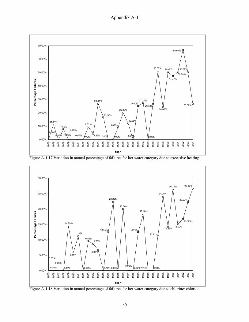
Appendix A-1
55
66.67%
26.67%
50.00%
50.00%
47.37%
27.27%
4.35%0.00%
24.00%
50.00%
26.67%
0.00%0.00%
0.00%
11.11%
0.00%
9.52%
0.00%
16.67%
0.00% 0.00%
9.09%
20.00%
12.00%
0.00%
25.00%
0.00%
50.00%
26.32%
7.69%
0.00%
10.00%
20.00%
30.00%
40.00%
50.00%
60.00%
70.00%19
75
1976
1977
1978
1979
1980
1981
1982
1983
1984
1985
1986
1987
1988
1989
1990
1991
1992
1993
1994
1995
1996
1997
1998
1999
2000
2001
2002
2003
2004
Year
Perc
enta
ge F
ailu
res
Figure A-1.17 Variation in annual percentage of failures for hot water category due to excessive heating
26.67%
22.22%
16.67%
15.00%
26.32%
18.18%
8.70%
11.11%
24.00%
14.29%
6.67%
14.29%
0.00%
0.00%
0.00% 0.00%
9.52%
5.88%
0.00%
12.50%
22.22%
0.00%
20.00%
0.00%0.00%
12.50%
0.00%
11.11%
0.00%0.00%0.00%
5.00%
10.00%
15.00%
20.00%
25.00%
30.00%
1975
1976
1977
1978
1979
1980
1981
1982
1983
1984
1985
1986
1987
1988
1989
1990
1991
1992
1993
1994
1995
1996
1997
1998
1999
2000
2001
2002
2003
2004
Year
Perc
enta
ge F
ailu
res
Figure A-1.18 Variation in annual percentage of failures for hot water category due to chlorine/ chloride

Appendix A-1
56
6.67%
11.11%
8.33%
10.00%
0.00%0.00%
8.70%
0.00%
12.00%
3.57%
13.33%14.29%
14.29%
0.00%
22.22%
15.38%
0.00%
11.76%
0.00%
12.50%
11.11%
27.27%
10.00%
16.00%
30.00%
12.50%
0.00%
11.11%
21.05%
23.08%
0.00%
5.00%
10.00%
15.00%
20.00%
25.00%
30.00%
35.00%19
75
1976
1977
1978
1979
1980
1981
1982
1983
1984
1985
1986
1987
1988
1989
1990
1991
1992
1993
1994
1995
1996
1997
1998
1999
2000
2001
2002
2003
2004
Year
Perc
enta
ge F
ailu
res
Figure A-1.19 Variation in annual percentage of failures for hot water category due to external failure
33.33%
11.11%
4.17%
10.00%
5.26%
18.18%
43.48%
38.89%
20.00%
10.71%
20.00%
0.00%
14.29%
62.50%
22.22%
46.15%
19.05%
29.41% 33.33%
50.00%
44.44%
27.27%
30.00%
16.00%
20.00%
12.50%
66.67%
0.00%
15.79%
15.38%
0.00%
10.00%
20.00%
30.00%
40.00%
50.00%
60.00%
70.00%
1975
1976
1977
1978
1979
1980
1981
1982
1983
1984
1985
1986
1987
1988
1989
1990
1991
1992
1993
1994
1995
1996
1997
1998
1999
2000
2001
2002
2003
2004
Year
Perc
enta
ge F
ailu
res
Figure A-1.20 Variation in annual percentage of failures for hot water category due to minor causes

Appendix A-1
57
Table A-1.1 Annual breakup of failures categorized by pipe types, CDA data (1975~2004) Pipe Type
Year
Number of reports
Cold Water
Hot Water Hydronic
Service Lines
Fire Suppression
Others/ Not known a
2004 40 19 13 2 4 0 3 46.34 31.71 4.88 9.76 0.00 7.32
2003 75 43 13 5 7 0 8 56.58 17.11 6.58 9.21 0.00 10.53
2002 64 31 19 5 8 2 4 44.93 27.54 7.25 11.59 2.90 5.80
2001 69 35 16 4 6 1 14 46.05 21.05 5.26 7.89 1.32 18.42
2000 79 50 15 4 6 1 7 60.24 18.07 4.82 7.23 1.20 8.43
1999 87 48 19 9 5 2 5 54.55 21.59 10.23 5.68 2.27 5.68
1998 62 22 19 6 13 1 4 33.85 29.23 9.23 20.00 1.54 6.15
1997 60 32 3 15 4 2 5 52.46 4.92 24.59 6.56 3.28 8.20
1996 46 17 7 12 2 2 7 36.17 14.89 25.53 4.26 4.26 14.89
1995 32 18 3 3 2 2 5 54.55 9.09 9.09 6.06 6.06 15.15
1994 32 13 5 6 2 3 3 40.63 15.63 18.75 6.25 9.38 9.38
1993 55 21 6 10 2 6 11 37.50 10.71 17.86 3.57 10.71 19.64
1992 32 5 4 6 4 1 12 15.63 12.50 18.75 12.50 3.13 37.50
1991 61 20 13 12 2 3 15 30.77 20.00 18.46 3.08 4.62 23.08
1990 23 10 5 5 1 0 5 38.46 19.23 19.23 3.85 0.00 19.23
1989 29 6 6 5 3 2 8 20.00 20.00 16.67 10.00 6.67 26.67
1988 23 6 3 6 1 2 6 25.00 12.50 25.00 4.17 8.33 25.00
Table continues on the next page

Appendix A-1
58
Table A-1.1 Annual breakup of failures categorized by pipe types, CDA data (1975~2004) Pipe Type
Year
Number of reports
Cold Water
Hot Water Hydronic
Service Lines
Fire Suppression
Others/ Not known a
1987 19 4 4 4 0 3 6 19.05 19.05 19.05 0.00 14.29 28.57
1986 21 8 3 3 1 3 5 34.78 13.04 13.04 4.35 13.04 21.74
1985 40 11 8 7 6 2 8 26.19 19.05 16.67 14.29 4.76 19.05
1984 52 26 14 9 6 0 9 40.63 21.88 14.06 9.38 0.00 14.06
1983 49 19 4 17 6 1 4 37.25 7.84 33.33 11.76 1.96 7.84
1982 44 18 2 11 6 0 8 40.00 4.44 24.44 13.33 0.00 17.78
1981 43 16 4 14 4 1 8 34.04 8.51 29.79 8.51 2.13 17.02
1980 44 18 2 15 3 0 7 40.00 4.44 33.33 6.67 0.00 15.56
1979 28 15 5 9 0 0 2 48.39 16.13 29.03 0.00 0.00 6.45
1978 39 22 5 8 2 0 4 53.66 12.20 19.51 4.88 0.00 9.76
1977 25 13 4 4 2 0 3 50.00 15.38 15.38 7.69 0.00 11.54
1976 21 10 8 1 0 0 4 43.48 34.78 4.35 0.00 0.00 17.39
1975 19 5 5 2 2 0 5 26.32 26.32 10.53 10.53 0.00 26.32
Total 1313 b 581 237 219 110 40 195Overall Average 42.04 17.15 15.85 7.96 2.89 14.11 The numbers in italics represent the percentage of the said attribute for that particular year. a These include the reports that did not contain any information about the pipe type, also this attribute includes cases from refrigerant pipes, drain pipes, solar heating systems. b The total number of reports is 1313, but the sum of the individual attributes will be more than this number as some reports contained failure reports for more than one type of pipes., such cases are counted twice (once for each attribute)
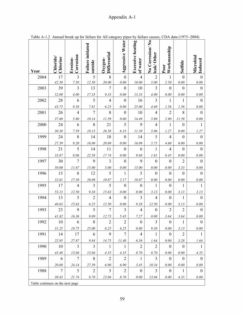
Appendix A-1
59
Table A-1.2 Annual break up for failure for All category pipes by failure causes, CDA data (1975~2004)
Year Chl
orid
e/
Chl
orin
e
Ero
sion
-C
orro
sion
Failu
re in
itiat
ed
outs
ide
Oxy
gen-
Diff
eren
tial
Agg
ress
ive
Wat
er
Exc
essi
ve h
eatin
g of
wat
er
No
Cor
rosi
on/ N
o le
ak/ O
ther
Poor
W
orkm
ansh
ip
Sulfi
de
Mic
robi
al
Indu
ced
2004 17 3 5 8 0 4 2 1 0 0 42.50 7.50 12.50 20.00 0.00 10.00 5.00 2.50 0.00 0.00
2003 39 3 13 7 0 10 3 0 0 0 52.00 4.00 17.33 9.33 0.00 13.33 4.00 0.00 0.00 0.00
2002 28 6 5 4 0 16 3 1 1 0 43.75 9.38 7.81 6.25 0.00 25.00 4.69 1.56 1.56 0.00
2001 26 4 7 8 0 10 4 2 8 0 37.68 5.80 10.14 11.59 0.00 14.49 5.80 2.90 11.59 0.00
2000 24 6 8 21 5 9 4 1 0 1 30.38 7.59 10.13 26.58 6.33 11.39 5.06 1.27 0.00 1.27
1999 24 8 14 18 0 14 5 4 0 0 27.59 9.20 16.09 20.69 0.00 16.09 5.75 4.60 0.00 0.00
1998 21 5 14 11 0 6 1 4 0 0 33.87 8.06 22.58 17.74 0.00 9.68 1.61 6.45 0.00 0.00
1997 30 7 9 3 0 9 0 0 2 0 50.00 11.67 15.00 5.00 0.00 15.00 0.00 0.00 3.33 0.00
1996 15 8 12 5 1 5 0 0 0 0 32.61 17.39 26.09 10.87 2.17 10.87 0.00 0.00 0.00 0.00
1995 17 4 3 5 0 0 1 0 1 1 53.13 12.50 9.38 15.63 0.00 0.00 3.13 0.00 3.13 3.13
1994 13 5 2 4 0 3 4 0 1 0 40.63 15.63 6.25 12.50 0.00 9.38 12.50 0.00 3.13 0.00
1993 23 9 5 7 3 4 0 2 2 0 41.82 16.36 9.09 12.73 5.45 7.27 0.00 3.64 3.64 0.00
1992 10 6 8 2 2 0 3 0 1 0 31.25 18.75 25.00 6.25 6.25 0.00 9.38 0.00 3.13 0.00
1991 14 17 6 9 7 4 1 0 2 1 22.95 27.87 9.84 14.75 11.48 6.56 1.64 0.00 3.28 1.64
1990 10 3 3 1 1 2 2 0 0 1 43.48 13.04 13.04 4.35 4.35 8.70 8.70 0.00 0.00 4.35
1989 6 7 8 2 2 1 3 0 0 0 20.69 24.14 27.59 6.90 6.90 3.45 10.34 0.00 0.00 0.00
1988 7 5 2 3 2 0 3 0 1 0 30.43 21.74 8.70 13.04 8.70 0.00 13.04 0.00 4.35 0.00
Table continues on the next page

Appendix A-1
60
Table A-1.2 Annual break up for failure for All category pipes by failure causes, CDA data (1975~2004)
Year Chl
orid
e/
Chl
orin
e
Ero
sion
-C
orro
sion
Failu
re in
itiat
ed
outs
ide
Oxy
gen-
Diff
eren
tial
Agg
ress
ive
Wat
er
Exc
essi
ve h
eatin
g of
wat
er
No
Cor
rosi
on/ N
o le
ak/ O
ther
Poor
W
orkm
ansh
ip
Sulfi
de
Mic
robi
al
Indu
ced
1987 4 2 2 4 1 0 5 0 1 0 21.05 10.53 10.53 21.05 5.26 0.00 26.32 0.00 5.26 0.00
1986 9 3 4 1 1 2 1 0 0 0 42.86 14.29 19.05 4.76 4.76 9.52 4.76 0.00 0.00 0.00
1985 14 8 3 3 3 6 2 0 1 0 35.00 20.00 7.50 7.50 7.50 15.00 5.00 0.00 2.50 0.00
1984 11 13 3 8 7 1 3 3 3 0 21.15 25.00 5.77 15.38 13.46 1.92 5.77 5.77 5.77 0.00
1983 4 14 5 2 13 2 4 4 1 0 8.16 28.57 10.20 4.08 26.53 4.08 8.16 8.16 2.04 0.00
1982 9 8 6 3 11 0 5 1 1 0 20.45 18.18 13.64 6.82 25.00 0.00 11.36 2.27 2.27 0.00
1981 6 11 3 2 10 0 7 2 2 0 13.95 25.58 6.98 4.65 23.26 0.00 16.28 4.65 4.65 0.00
1980 5 12 5 1 15 0 4 2 0 0 11.36 27.27 11.36 2.27 34.09 0.00 9.09 4.55 0.00 0.00
1979 3 13 2 0 8 0 2 0 0 0 10.71 46.43 7.14 0.00 28.57 0.00 7.14 0.00 0.00 0.00
1978 2 11 6 2 16 1 1 0 0 0 5.13 28.21 15.38 5.13 41.03 2.56 2.56 0.00 0.00 0.00
1977 1 7 4 0 10 0 2 1 0 0 4.00 28.00 16.00 0.00 40.00 0.00 8.00 4.00 0.00 0.00
1976 0 6 2 0 7 1 5 0 0 0 0.00 28.57 9.52 0.00 33.33 4.76 23.81 0.00 0.00 0.00
1975 0 10 3 0 3 0 2 1 0 0 0.00 52.63 15.79 0.00 15.79 0.00 10.53 5.26 0.00 0.00 Total = 1313 392 224 172 144 128 110 82 c 29 28 4Overall Average 29.86 17.06 13.10 10.97 9.75 8.38 6.25 2.21 2.13 0.30 The numbers in italics represent the percentage of the said attribute for that particular year. The data presented contain the reports for all categories of pipe (hot water, hydronic, cold water, service lines, fire suppression and all pipes under unknown category). The segregation based on pipe categories is presented in subsequent tables. c The number includes cases in which the failure cause was not established, or when the sample of pipe was drawn to study complaints about “Blue water” but there was no leak in the pipe. The data is presented in figures 4 through 13.
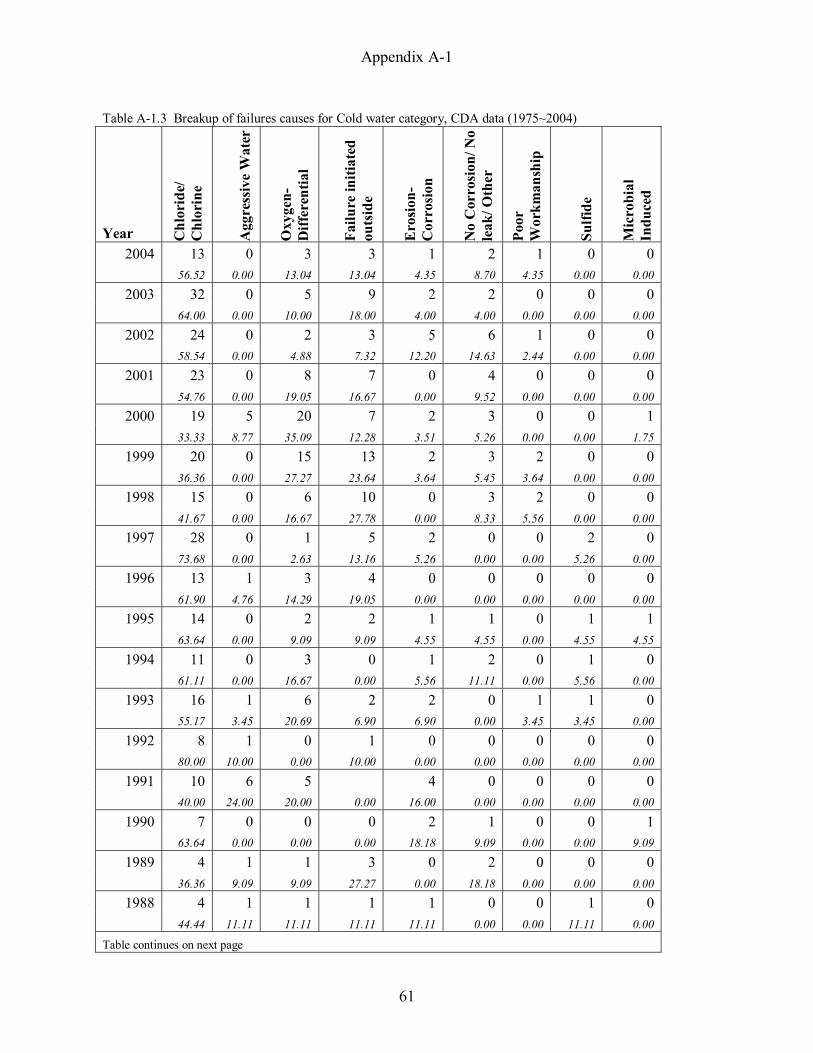
Appendix A-1
61
Table A-1.3 Breakup of failures causes for Cold water category, CDA data (1975~2004)
Year Chl
orid
e/
Chl
orin
e
Agg
ress
ive
Wat
er
Oxy
gen-
Diff
eren
tial
Failu
re in
itiat
ed
outs
ide
Ero
sion
-C
orro
sion
No
Cor
rosi
on/ N
o le
ak/ O
ther
Poor
W
orkm
ansh
ip
Sulfi
de
Mic
robi
al
Indu
ced
2004 13 0 3 3 1 2 1 0 0 56.52 0.00 13.04 13.04 4.35 8.70 4.35 0.00 0.00
2003 32 0 5 9 2 2 0 0 0 64.00 0.00 10.00 18.00 4.00 4.00 0.00 0.00 0.00
2002 24 0 2 3 5 6 1 0 0 58.54 0.00 4.88 7.32 12.20 14.63 2.44 0.00 0.00
2001 23 0 8 7 0 4 0 0 0 54.76 0.00 19.05 16.67 0.00 9.52 0.00 0.00 0.00
2000 19 5 20 7 2 3 0 0 1 33.33 8.77 35.09 12.28 3.51 5.26 0.00 0.00 1.75
1999 20 0 15 13 2 3 2 0 0 36.36 0.00 27.27 23.64 3.64 5.45 3.64 0.00 0.00
1998 15 0 6 10 0 3 2 0 0 41.67 0.00 16.67 27.78 0.00 8.33 5.56 0.00 0.00
1997 28 0 1 5 2 0 0 2 0 73.68 0.00 2.63 13.16 5.26 0.00 0.00 5.26 0.00
1996 13 1 3 4 0 0 0 0 0 61.90 4.76 14.29 19.05 0.00 0.00 0.00 0.00 0.00
1995 14 0 2 2 1 1 0 1 1 63.64 0.00 9.09 9.09 4.55 4.55 0.00 4.55 4.55
1994 11 0 3 0 1 2 0 1 0 61.11 0.00 16.67 0.00 5.56 11.11 0.00 5.56 0.00
1993 16 1 6 2 2 0 1 1 0 55.17 3.45 20.69 6.90 6.90 0.00 3.45 3.45 0.00
1992 8 1 0 1 0 0 0 0 0 80.00 10.00 0.00 10.00 0.00 0.00 0.00 0.00 0.00
1991 10 6 5 4 0 0 0 0 40.00 24.00 20.00 0.00 16.00 0.00 0.00 0.00 0.00
1990 7 0 0 0 2 1 0 0 1 63.64 0.00 0.00 0.00 18.18 9.09 0.00 0.00 9.09
1989 4 1 1 3 0 2 0 0 0 36.36 9.09 9.09 27.27 0.00 18.18 0.00 0.00 0.00
1988 4 1 1 1 1 0 0 1 0 44.44 11.11 11.11 11.11 11.11 0.00 0.00 11.11 0.00
Table continues on next page

Appendix A-1
62
Table A-1.3 Breakup of failures causes for Cold water category, CDA data (1975~2004)
Year Chl
orid
e/
Chl
orin
e
Agg
ress
ive
Wat
er
Oxy
gen-
Diff
eren
tial
Failu
re in
itiat
ed
outs
ide
Ero
sion
-C
orro
sion
No
Cor
rosi
on/ N
o le
ak/ O
ther
Poor
W
orkm
ansh
ip
Sulfi
de
Mic
robi
al
Indu
ced
1987 3 1 1 0 1 1 0 0 0 42.86 14.29 14.29 0.00 14.29 14.29 0.00 0.00 0.00
1986 6 1 0 4 1 0 0 0 0 50.00 8.33 0.00 33.33 8.33 0.00 0.00 0.00 0.00
1985 12 3 1 0 2 1 0 0 0 63.16 15.79 5.26 0.00 10.53 5.26 0.00 0.00 0.00
1984 11 6 3 1 6 2 2 1 0 34.38 18.75 9.38 3.13 18.75 6.25 6.25 3.13 0.00
1983 2 12 2 4 2 2 1 1 0 7.69 46.15 7.69 15.38 7.69 7.69 3.85 3.85 0.00
1982 8 11 1 2 0 0 1 1 0 33.33 45.83 4.17 8.33 0.00 0.00 4.17 4.17 0.00
1981 3 8 1 3 3 1 1 1 0 14.29 38.10 4.76 14.29 14.29 4.76 4.76 4.76 0.00
1980 4 11 1 2 3 0 0 0 19.05 52.38 0.00 4.76 9.52 14.29 0.00 0.00 0.00
1979 1 8 0 0 5 1 0 0 0 6.67 53.33 0.00 0.00 33.33 6.67 0.00 0.00 0.00
1978 1 14 1 2 5 1 0 0 0 4.17 58.33 4.17 8.33 20.83 4.17 0.00 0.00 0.00
1977 0 8 0 3 4 0 0 0 0 0.00 53.33 0.00 20.00 26.67 0.00 0.00 0.00 0.00
1976 0 6 0 0 2 2 0 0 0 0.00 60.00 0.00 0.00 20.00 20.00 0.00 0.00 0.00
1975 0 2 0 0 3 1 1 0 0 0.00 28.57 0.00 0.00 42.86 14.29 14.29 0.00 0.00 Total =731 312 107 91 90 61 d 44 d 13 d 10 d 3 d
Overall Average 42.68 14.64 12.45 12.31 8.34 6.02 1.78 1.37 0.41 The numbers in italics represent the percentage of the said attribute for that particular year. d These attributes are categorized as minor causes and are shown together in figures. The data is presented in figures

Appendix A-1
63
Table A-1.4 Breakup of failure causes for Hot water category, CDA data (1975~2004)
Year Ero
sion
-C
orro
sion
Exc
essi
ve h
eatin
g of
wat
er
Chl
orid
e/
Chl
orin
e
Failu
re in
itiat
ed
outs
ide
Oxy
gen-
Diff
eren
tial
No
Cor
rosi
on/ N
o le
ak/ O
ther
Agg
ress
ive
Wat
er
Poor
W
orkm
ansh
ip
Sulfi
de
Mic
robi
al
Indu
ced
2004 1 4 4 1 4 1 0 0 0 0 6.67 26.67 26.67 6.67 26.67 6.67 0.00 0.00 0.00 0.00
2003 1 9 4 2 1 1 0 0 0 0 5.56 50.00 22.22 11.11 5.56 5.56 0.00 0.00 0.00 0.00
2002 1 16 4 2 1 0 0 0 0 0 4.17 66.67 16.67 8.33 4.17 0.00 0.00 0.00 0.00 0.00
2001 3 10 3 2 0 1 0 1 0 0 15.00 50.00 15.00 10.00 0.00 5.00 0.00 5.00 0.00 0.00
2000 4 9 5 0 0 0 0 1 0 0 21.05 47.37 26.32 0.00 0.00 0.00 0.00 5.26 0.00 0.00
1999 6 14 4 1 0 3 0 0 0 0 21.43 50.00 14.29 3.57 0.00 10.71 0.00 0.00 0.00 0.00
1998 5 6 6 3 3 0 0 2 0 0 20.00 24.00 24.00 12.00 12.00 0.00 0.00 8.00 0.00 0.00
1997 5 9 2 2 0 0 0 0 0 0 27.78 50.00 11.11 11.11 0.00 0.00 0.00 0.00 0.00 0.00
1996 7 5 0 4 3 0 0 0 0 0 36.84 26.32 0.00 21.05 15.79 0.00 0.00 0.00 0.00 0.00
1995 2 0 0 0 4 0 0 0 0 0 33.33 0.00 0.00 0.00 66.67 0.00 0.00 0.00 0.00 0.00
1994 4 3 2 0 1 1 0 0 0 0 36.36 27.27 18.18 0.00 9.09 9.09 0.00 0.00 0.00 0.00
1993 6 4 2 2 1 0 0 1 0 0 37.50 25.00 12.50 12.50 6.25 0.00 0.00 6.25 0.00 0.00
1992 5 0 3 1 1 0 0 0 0 50.00 0.00 0.00 30.00 10.00 10.00 0.00 0.00 0.00 0.00
1991 14 3 0 4 3 0 0 0 0 1 56.00 12.00 0.00 16.00 12.00 0.00 0.00 0.00 0.00 4.00
1990 2 2 2 1 1 2 0 0 0 0 20.00 20.00 20.00 10.00 10.00 20.00 0.00 0.00 0.00 0.00
1989 4 1 0 3 1 1 1 0 0 0 36.36 9.09 0.00 27.27 9.09 9.09 9.09 0.00 0.00 0.00
1988 2 0 2 1 2 2 0 0 0 0 22.22 0.00 22.22 11.11 22.22 22.22 0.00 0.00 0.00 0.00
Table continues on the next page
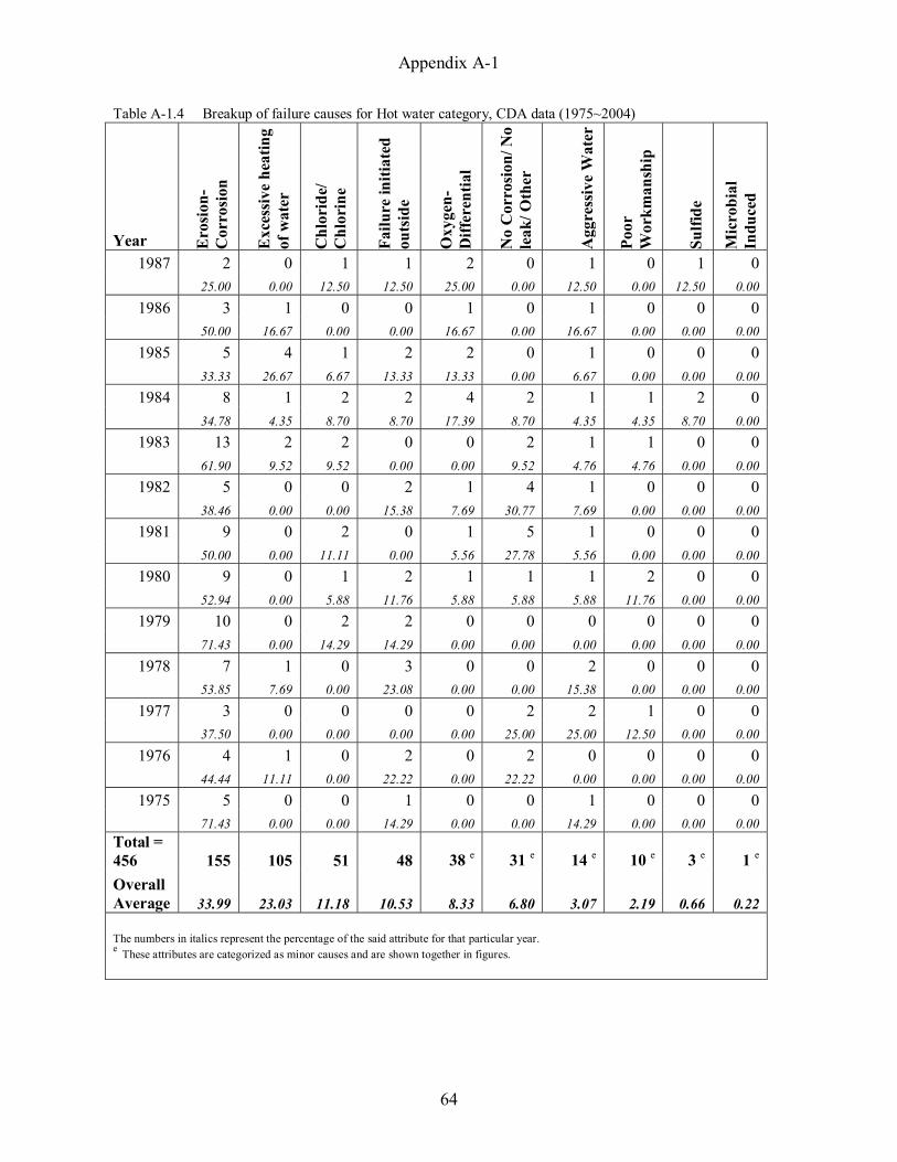
Appendix A-1
64
Table A-1.4 Breakup of failure causes for Hot water category, CDA data (1975~2004)
Year Ero
sion
-C
orro
sion
Exc
essi
ve h
eatin
g of
wat
er
Chl
orid
e/
Chl
orin
e
Failu
re in
itiat
ed
outs
ide
Oxy
gen-
Diff
eren
tial
No
Cor
rosi
on/ N
o le
ak/ O
ther
Agg
ress
ive
Wat
er
Poor
W
orkm
ansh
ip
Sulfi
de
Mic
robi
al
Indu
ced
1987 2 0 1 1 2 0 1 0 1 0 25.00 0.00 12.50 12.50 25.00 0.00 12.50 0.00 12.50 0.00
1986 3 1 0 0 1 0 1 0 0 0 50.00 16.67 0.00 0.00 16.67 0.00 16.67 0.00 0.00 0.00
1985 5 4 1 2 2 0 1 0 0 0 33.33 26.67 6.67 13.33 13.33 0.00 6.67 0.00 0.00 0.00
1984 8 1 2 2 4 2 1 1 2 0 34.78 4.35 8.70 8.70 17.39 8.70 4.35 4.35 8.70 0.00
1983 13 2 2 0 0 2 1 1 0 0 61.90 9.52 9.52 0.00 0.00 9.52 4.76 4.76 0.00 0.00
1982 5 0 0 2 1 4 1 0 0 0 38.46 0.00 0.00 15.38 7.69 30.77 7.69 0.00 0.00 0.00
1981 9 0 2 0 1 5 1 0 0 0 50.00 0.00 11.11 0.00 5.56 27.78 5.56 0.00 0.00 0.00
1980 9 0 1 2 1 1 1 2 0 0 52.94 0.00 5.88 11.76 5.88 5.88 5.88 11.76 0.00 0.00
1979 10 0 2 2 0 0 0 0 0 0 71.43 0.00 14.29 14.29 0.00 0.00 0.00 0.00 0.00 0.00
1978 7 1 0 3 0 0 2 0 0 0 53.85 7.69 0.00 23.08 0.00 0.00 15.38 0.00 0.00 0.00
1977 3 0 0 0 0 2 2 1 0 0 37.50 0.00 0.00 0.00 0.00 25.00 25.00 12.50 0.00 0.00
1976 4 1 0 2 0 2 0 0 0 0 44.44 11.11 0.00 22.22 0.00 22.22 0.00 0.00 0.00 0.00
1975 5 0 0 1 0 0 1 0 0 0 71.43 0.00 0.00 14.29 0.00 0.00 14.29 0.00 0.00 0.00 Total = 456 155 105 51 48 38 e 31 e 14 e 10 e 3 e 1 e
Overall Average 33.99 23.03 11.18 10.53 8.33 6.80 3.07 2.19 0.66 0.22 The numbers in italics represent the percentage of the said attribute for that particular year. e These attributes are categorized as minor causes and are shown together in figures.

Appendix A-1
65
Table A-1.5 Breakup of failure causes for others/ unknown category, CDA data (1975~2004)
Year Failu
re in
itiat
ed
outs
ide
Chl
orid
e/
Chl
orin
e
No
Cor
rosi
on/
No
leak
/ Oth
er
Ero
sion
-C
orro
sion
Oxy
gen-
Diff
eren
tial
Sulfi
de
Agg
ress
ive
Wat
er
Poor
W
orkm
ansh
ip
Exc
essi
ve
heat
ing
of w
ater
2004 1 0 0 1 1 0 0 0 0 33.33 0.00 0.00 33.33 33.33 0.00 0.00 0.00 0.00
2003 2 3 1 0 1 0 0 0 1 25.00 37.50 12.50 0.00 12.50 0.00 0.00 0.00 12.50
2002 0 0 2 0 1 1 0 0 0 0.00 0.00 50.00 0.00 25.00 25.00 0.00 0.00 0.00
2001 1 0 3 1 0 8 0 1 0 7.14 0.00 21.43 7.14 0.00 57.14 0.00 7.14 0.00
2000 3 0 3 0 1 0 0 0 0 42.86 0.00 42.86 0.00 14.29 0.00 0.00 0.00 0.00
1999 0 0 0 0 3 0 0 2 0 0.00 0.00 0.00 0.00 60.00 0.00 0.00 40.00 0.00
1998 1 0 1 0 2 0 0 0 0 25.00 0.00 25.00 0.00 50.00 0.00 0.00 0.00 0.00
1997 2 1 0 0 2 0 0 0 0 40.00 20.00 0.00 0.00 40.00 0.00 0.00 0.00 0.00
1996 4 2 0 1 0 0 0 0 0 57.14 28.57 0.00 14.29 0.00 0.00 0.00 0.00 0.00
1995 1 3 0 1 0 0 0 0 0 20.00 60.00 0.00 20.00 0.00 0.00 0.00 0.00 0.00
1994 2 0 1 0 0 0 0 0 0 66.67 0.00 33.33 0.00 0.00 0.00 0.00 0.00 0.00
1993 1 6 0 1 0 1 2 0 0 9.09 54.55 0.00 9.09 0.00 9.09 18.18 0.00 0.00
1992 4 2 2 1 1 1 1 0 0 33.33 16.67 16.67 8.33 8.33 8.33 8.33 0.00 0.00
1991 2 4 1 2 2 2 1 0 1 13.33 26.67 6.67 13.33 13.33 13.33 6.67 0.00 6.67
1990 2 2 0 0 0 0 1 0 0 40.00 40.00 0.00 0.00 0.00 0.00 20.00 0.00 0.00
1989 2 2 0 3 0 0 1 0 0 25.00 25.00 0.00 37.50 0.00 0.00 12.50 0.00 0.00
1988 0 2 1 2 0 0 1 0 0 0.00 33.33 16.67 33.33 0.00 0.00 16.67 0.00 0.00
Table continues on next page
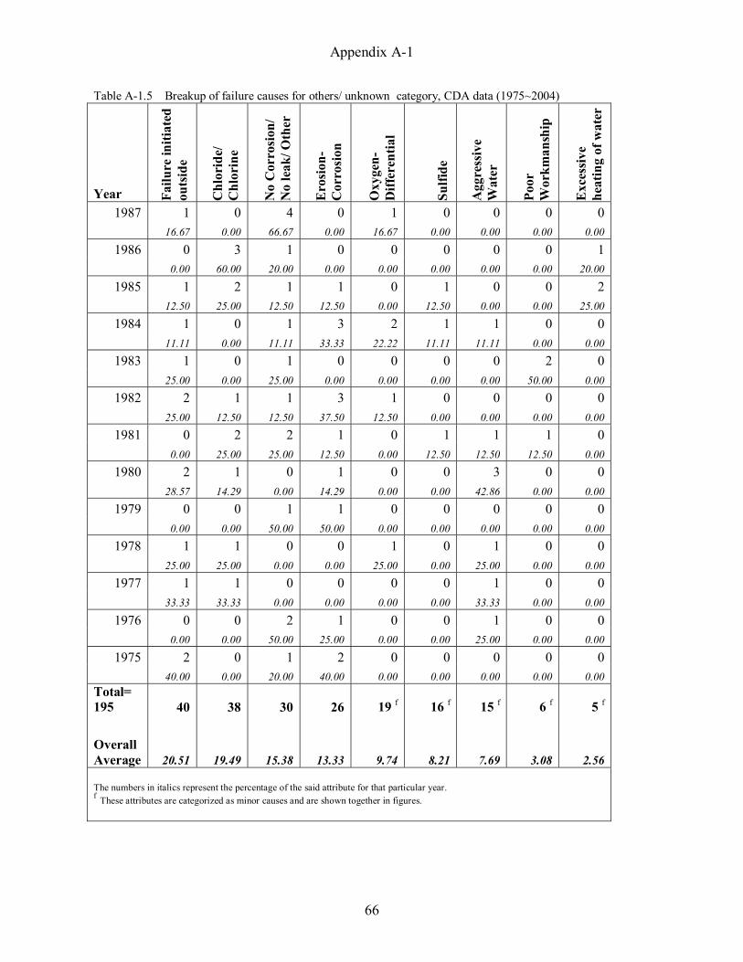
Appendix A-1
66
Table A-1.5 Breakup of failure causes for others/ unknown category, CDA data (1975~2004)
Year Failu
re in
itiat
ed
outs
ide
Chl
orid
e/
Chl
orin
e
No
Cor
rosi
on/
No
leak
/ Oth
er
Ero
sion
-C
orro
sion
Oxy
gen-
Diff
eren
tial
Sulfi
de
Agg
ress
ive
Wat
er
Poor
W
orkm
ansh
ip
Exc
essi
ve
heat
ing
of w
ater
1987 1 0 4 0 1 0 0 0 0 16.67 0.00 66.67 0.00 16.67 0.00 0.00 0.00 0.00
1986 0 3 1 0 0 0 0 0 1 0.00 60.00 20.00 0.00 0.00 0.00 0.00 0.00 20.00
1985 1 2 1 1 0 1 0 0 2 12.50 25.00 12.50 12.50 0.00 12.50 0.00 0.00 25.00
1984 1 0 1 3 2 1 1 0 0 11.11 0.00 11.11 33.33 22.22 11.11 11.11 0.00 0.00
1983 1 0 1 0 0 0 0 2 0 25.00 0.00 25.00 0.00 0.00 0.00 0.00 50.00 0.00
1982 2 1 1 3 1 0 0 0 0 25.00 12.50 12.50 37.50 12.50 0.00 0.00 0.00 0.00
1981 0 2 2 1 0 1 1 1 0 0.00 25.00 25.00 12.50 0.00 12.50 12.50 12.50 0.00
1980 2 1 0 1 0 0 3 0 0 28.57 14.29 0.00 14.29 0.00 0.00 42.86 0.00 0.00
1979 0 0 1 1 0 0 0 0 0 0.00 0.00 50.00 50.00 0.00 0.00 0.00 0.00 0.00
1978 1 1 0 0 1 0 1 0 0 25.00 25.00 0.00 0.00 25.00 0.00 25.00 0.00 0.00
1977 1 1 0 0 0 0 1 0 0 33.33 33.33 0.00 0.00 0.00 0.00 33.33 0.00 0.00
1976 0 0 2 1 0 0 1 0 0 0.00 0.00 50.00 25.00 0.00 0.00 25.00 0.00 0.00
1975 2 0 1 2 0 0 0 0 0 40.00 0.00 20.00 40.00 0.00 0.00 0.00 0.00 0.00 Total= 195 40 38 30 26 19 f 16 f 15 f 6 f 5 f
Overall Average 20.51 19.49 15.38 13.33 9.74 8.21 7.69 3.08 2.56 The numbers in italics represent the percentage of the said attribute for that particular year. f These attributes are categorized as minor causes and are shown together in figures.

Appendix B-1
67
APPENDIX B-1
Temporal Patterns of Pinhole Leaks by Pipe Characteristics
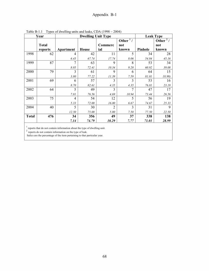
Appendix B-1
68
Table B-1.1 Types of dwelling units and leaks, CDA (1998 ~ 2004)
Year Dwelling Unit Type Leak Type
Total reports Apartment House
Commercial
Other 1 / not known Pinhole
Other 2 / not known
62 4 42 11 5 34 281998 6.45 67.74 17.74 8.06 54.84 45.16
87 7 63 9 8 53 341999 8.05 72.41 10.34 9.20 60.92 39.08
79 3 61 9 6 64 152000 3.80 77.22 11.39 7.59 81.01 18.99)
69 6 57 3 3 53 162001 8.70 82.61 4.35 4.35 76.81 23.19
64 5 49 3 7 47 172002 7.81 76.56 4.69 10.94 73.44 26.56
75 4 54 12 5 56 192003 5.33 72.00 16.00 6.67 74.67 25.33
40 5 30 2 3 31 92004 12.50 75.00 5.00 7.50 77.50 22.50
476 34 356 49 37 338 138Total 7.14 74.79 10.29 7.77 71.01 28.99
1 reports that do not contain information about the type of dwelling unit. 2 reports do not contain information on the type of leak. Italics are the percentage of the item pertaining to that particular year.

Appendix B-1
69
Table B-1.2 Types of pipes and pipe orientation, CDA (1998~2004) Year Pipe Type Pipe Orientation
K-type L-type M-type
Other / not known 3 Horizontal Vertical
Not Known
9 30 23 2 25 5 331998 14.06 46.88 35.94 3.13 39.68 7.94 52.38
7 41 39 3 46 12 321999 7.78 45.56 43.33 3.33 51.11 13.33 35.56
6 31 44 3 42 9 322000 7.14 36.90 52.38 3.57 50.60 10.84 38.55
6 30 31 3 22 5 422001 8.57 42.86 44.29 4.29 31.88 7.25 60.87
6 29 29 1 31 4 292002 9.23 44.62 44.62 1.54 48.44 6.25 45.31
6 37 31 3 30 8 372003 7.79 48.05 40.26 3.90 40.00 10.67 49.33
5 20 15 1 19 6 162004 12.20 48.78 36.59 2.44 46.34 14.63 39.02
Total 4 45 218 212 16 215 49 221 9.16 44.40 43.18 3.26 44.33 10.10 45.57
3 pipe category other than plumbing pipe or not reported. 4 total may vary from the total number of CDA reports due to multiple items reported in some reports. Some reports have both M
and L types of failure and such cases are counted twice. Italics are the percentage of the item pertaining to that particular year.

Appendix B-1
70
Table B-1.3 Source of water and pipe sizes, CDA (1998~2004) Pipe Size (nominal diameter-inches) Source of Water
Year 0.5 0.75 1 Other 5 Ground water
Surface water
Other / not known
21 31 8 12 23 5 34 1998 29.17 43.06 11.11 16.67 37.10 8.06 54.84
40 30 12 13 45 15 34 1999 42.11 31.58 12.63 13.68 47.87 15.96 36.17
25 43 6 11 42 16 23 2000 29.41 50.59 7.06 12.94 51.85 19.75 28.40
32 25 7 10 33 19 18 2001 43.24 33.78 9.46 13.51 47.14 27.14 25.71
25 29 10 10 34 7 23 2002 33.78 39.19 13.51 13.51 53.13 10.94 35.94
32 30 7 10 34 22 22 2003 40.51 37.97 8.86 12.66 43.59 28.21 28.21
17 16 4 5 13 10 19 2004 40.48 38.10 9.52 11.90 30.95 23.81 45.24 Total 6 192 204 54 71 224 94 173 36.85 39.16 10.36 13.63 45.62 19.14 35.23
5 other pipe sizes and pipes are from heating systems, refrigerant systems etc. 6 total may vary from the total number of CDA reports due to multiple items reported. Some reports contain multiple sizes of failed pipes, such cases are counted twice. Italics contain the percentage of the item pertaining to the particular year.

71
CHAPTER-2
CAUSAL ANALYSIS OF PINHOLE LEAKS
Introduction
Corrosion is an electrochemical process; by definition it requires the presence of four
basic ingredients, an anode, a cathode, an electrolyte and a physical connection. All these four
ingredients facilitate an electrochemical reaction in which the anode is consumed due to loss of
metal whereas deposition occurs at cathode. By means of corrosion, the metals achieve higher
oxidation states that are thermodynamically more stable. Copper metal is oxidized to the cuprous
(+1) and cupric (+2) oxidation states in corrosion. A detailed overview of the thermodynamics
and kinetics of the corrosion phenomenon is presented in Chapter 4. The nature and type of
corrosion is highly dependant on the conditions of exposure and the environment. A summary of
the different types of corrosion of copper is given in Appendix A-2.
In general, when metals are exposed to oxygen, they tend to form a protective oxide film.
The film thus formed is usually thin and may not be visible to naked eye. The role of film is
particularly important in corrosion mechanism as it virtually forms a physical barrier between the
bare metal and the environment. However, the formation of the protective film does not
guarantee protection against corrosion, but it at least slows down the corrosion mechanism. The
extent to which the film may provide protection to the metal is highly dependent on its
conditions of exposure, for instance, the protective film may become soluble under certain
conditions thus leaving the metal unprotected.
72
In addition to the protective oxide film, other deposits may form on the surface of the metal.
These deposits or scales are primarily metal salts, and are the direct result of the reaction of the
metal with the constituents of its environment. The scales thus formed on the metal surface may
be protective, non protective or even corrosive depending upon the morphology, anions in the
solution and other environmental conditions including pH, temperature, alkalinity, velocity,
pressure etc. The role of the scales is extremely important in understanding corrosion
phenomenon; especially the scale seems to have a dominant role in copper pitting in home
plumbing systems.
The chapter synthesizes various physical, chemical factors that can lead to pinhole leaks in
copper home plumbing. The objectives of the chapter are:
i. Assess the variability in water quality based on nationwide water quality data from
AWWARF/ AWWA utilities.
ii. Identify and summarize physical and chemical parameters that influence copper pitting in
home plumbing systems.
iii. Identify the causal mechanisms in terms of the water quality and hydraulic parameters and
quantify these parameters based on the likelihood of copper pitting.
iv. Develop a scoring system for water quality and hydraulic parameters that influence pinhole
leak.

73
Overview of Water Quality
Almost all the home plumbing systems withdraw water from large municipal distribution
systems. These large distributions systems are managed and operated by public or private
utilities. The utilities withdraw water either from surface water bodies (i.e. lakes, springs and
rivers) or from ground water aquifers or a combination of both. The water obtained from either
surface or ground source is called raw water, it is then passed through a set of treatment stages at
the treatment plant before it is sent into the distribution system. The treatment plants are
generally located at or near the water source bodies and are typically far from residential
establishments. The treated water or the finished water is then pumped into the bigger
distribution system where it is conveyed through a system of pipe network. The branched
network extends to street and service laterals that finally get connected to the home plumbing
systems.
The quality of the raw water is dependant on the source from where it is withdrawn. In
general, surface waters are more turbid as compared to ground waters (Tchobanoglous, 1985).
Surface waters also have more organic contaminants and contain urban pollutants that reach the
surface water bodies with surface runoff. Ground waters on the other hand, have higher TDS
(total dissolved solids) because of mineral pickup from soil and rocks (Tchobanoglous, 1985).
Ground waters may have dissolved gases like carbon dioxide [CO2], ammonia [NH3], hydrogen
sulfide [H2S] and sometimes iron and manganese.

74
In general, raw water contains impurities that are to be removed during the treatment
process. These impurities may be classified into organic and inorganic impurities. Organic
impurities include impurities due to the decay of natural vegetative and animal matter; these
impurities are often found in surface water, where these are brought into with the surface runoff.
The impurities include organic contaminant from urban and industrial establishments. The most
common problems associated with the organic impurities include color formation, taste and odor
issues, interference with water treatment process and formation of halogenated compounds
during chlorination (Tchobanoglous, 1985). The amount of organic impurities present in most of
the natural water is low (Tchobanoglous, 1985). The inorganic impurities can be classified into
ionic and non ionic species. The principal ionic species typically found in waters are Calcium
[Ca2+], Magnesium [Mg2+], Sodium [Na+], Potassium [K+] (as cations) and Bicarbonate [HCO3-],
Sulfate [SO42-], Chloride [Cl-] and Nitrate [NO3
-] (as anions). The most abundant compounds are
Bicarbonate, Sulfate and Chlorides of Calcium, Magnesium and Sodium (Tchobanoglous, 1985).
The non ionic inorganic impurity present in most of the water is Silica, which is usually present
as Silicon Dioxide [SiO2]. These organic and inorganic impurities need treatment prior to
sending the water in distribution system. The USEPA has set primary and secondary standards
for the finished water, to which the utilities should comply before supplying the water.
The national primary and secondary standards for drinking water are available on
http://www.epa.gov/safewater/mcl.html. The national primary standards are legally enforceable
standards, these consist of the list of contaminants that may have ill effects on public health, the
standards define permissible limits for these contaminants in public water systems, and these
limits are termed as maximum contaminant level (MCL). The principal categories identified

75
under primary standards include microorganisms, disinfection byproducts, disinfectants,
inorganic chemicals, organic chemicals and radionuclides. Interestingly, the primary standards
identify residual disinfectants as a contaminant that can affect public health. The standards set
permissible limits for maximum residual disinfectant level (MRDL), which is the highest level of
residual disinfectant in water.
The secondary standards are not legally enforceable standards. These standards consist
of the list of contaminants that may cause cosmetic hazards (skin or tooth discoloration), or may
have aesthetics ill effects (taste, color and odor issues) in drinking water. These standards are
recommendations by the USEPA, and are not enforced on public water systems. However, the
states may choose to make these standards as legally enforceable. The secondary contaminant list
with the possible ill effects is reproduced in Table 1.
In addition to primary and secondary standards, USEPA also identifies certain
contaminants that are presently not subjected to any regulation but are anticipated to occur in
public water systems and may require regulations under safe drinking water act (SDWA). These
contaminants are identified under unregulated category (http://www.epa.gov/safewater/mcl.html)

76
Table 1 Secondary maximum contaminant level (source USEPA) Contaminant Secondary MCL Noticeable Effects above the
Secondary MCL
Aluminum 0.05 to 0.2 mg/L* colored water Chloride 250 mg/L salty taste Color 15 color units visible tint Copper 1.0 mg/L metallic taste; blue-green staining Corrosivity Non-corrosive metallic taste; corroded pipes/ fixtures
staining Fluoride 2.0 mg/L tooth discoloration Foaming agents 0.5 mg/L frothy, cloudy; bitter taste; odor Iron 0.3 mg/L rusty color; sediment; metallic taste;
reddish or orange staining Manganese 0.05 mg/L black to brown color; black staining;
bitter metallic taste Odor 3 TON (threshold odor number) "rotten-egg", musty or chemical smell pH
6.5 - 8.5
low pH: bitter metallic taste; corrosion high pH: slippery feel; soda taste; deposits
Silver 0.1 mg/L skin discoloration; graying of the white part of the eye
Sulfate 250 mg/L salty taste Total Dissolved
Solids 500 mg/L hardness; deposits; colored water; staining; salty taste
Zinc 5 mg/L metallic taste * mg/L is milligrams of substance per liter of water
Interestingly, some of the contaminants in the secondary list are often considered
responsible for copper pitting, these include, Aluminum, Chloride, Sulfate, pH, Iron and
Manganese. A detailed discussion about the effect of these parameters on copper pitting is
presented later in the chapter. Since the secondary standards are not legally enforceable, it is
expected that there should be considerable variability in these parameters across different
utilities.

77
The finished water from the plant has to travel considerable distance through the
distribution system before entering the home plumbing systems. The distribution system
generally is comprised of pipes of various materials (e.g. Cast Iron, Reinforced Concrete,
Plastics etc), these pipes can have several kinds of deposits on their inner surfaces. The deposits
may be due to corrosion of these pipes, settling of silt or both. These deposits not only reduce the
hydraulic efficiency of the distribution system but can also shield microorganisms from
disinfectants. In order to check the unwanted growth of microorganism in the distribution
system, certain utilities provide disinfectant booster doses at suitable locations (booster stations)
in the bigger distribution system. Additionally, the pipes in distribution system can leach
chemicals into water thus changing the water chemistry. For instance, leaching of Aluminum and
Silica compounds from reinforced concrete pipes is a common concern. Considering the
complexity and nature of the interaction of finished water within the distribution system it may
be safer to assume that water entering the home plumbing system is different from the finished
water.
Hence, the actual variability in the quality parameters of the water that reach the home
plumbing system is expected to be much more than the variability in water quality of the finished
water. A review of the water quality data for 898 AWWA utilities demonstrates considerable
variability in water quality parameters for finished water on a nationwide scale. The summary of
the analysis of water quality data from AWWARF/AWWA utility survey (WATER:\STATS 1996
survey) is presented.

78
AWWARF/AWWA Utility Survey
WATER:\STATS is a joint cooperative effort between American Water Works Association
(AWWA) and American Water Works Association Research Foundation (AWWARF). It
consists of survey information from AWWA member utilities. The last survey was conducted in
the year 1996, 898 utilities responded to the survey out of a total of 3200 AWWA member
utilities. The database includes information about financial and revenue records, water treatment
and disposal practices, finished water quality parameters at the plant, and water quality
information in the distribution system. The database is available on payment on
http://www.awwa.org/Communications/h20stats/PriceTab.cfm.
Out of 898 water utilities that responded to the survey, (370) three hundred seventy are
ground water utilities, (284) two hundred eighty four are surface water utilities, (140) one
hundred forty are combined surface and ground water utilities, and (104) one hundred four are
the utilities that responded to the survey but did not provide any information for either ground
water or surface water. The database is segregated into six different spreadsheets; each
spreadsheet consists of number of worksheets that typically contain information for the
respondent utilities designated by an (R) in the title and all utilities designated by an (A) in the
title. The respondent utilities are the ones that responded to each question of the survey, while all
utilities contain all of the utilities that participated in the survey, even if they did not answer the
corresponding question for that worksheet. Each utility is identified with a unique identification
number in the database. Additionally, surface water utilities are also assigned a unique plant
identification number for different treatment plants (if more than one) under the same utility
79
identification number. For ground water utilities, the data is averaged across all the wells and
hence, no separate plant identification number is assigned.
The first spreadsheet contains revenue information of the utilities. It includes information
about the population served, service area, future water demand, ownership category (public/
private), ownership type (Municipal / investor/ State or Water District etc), present budgetary
conditions (asset / liability), average day production, other services provided etc. The
information is further segregated for ground and surface water utilities. The data in the
spreadsheet is helpful for business planning and analysis purposes; hence it is not included in the
present study.
The second spreadsheet contains data related to treatment practices, residuals and residual
disposal for water utilities. The data includes information about the present and planned
treatment practices for various treatment stages like raw storage, aeration, pre disinfection
oxidation, coagulation & flocculation, filtration, disinfection, corrosion control, finished water
storage etc for each utility. The data is segregated for ground and surface water utilities. The data
may be of interest from water treatment and waste disposal perspective, hence it is not included
in the present study.
The third spreadsheet contains data about the pipe materials for service lines and fire
lines for the utilities. The pipe material data for the water mains and year wise number of
breakages for the last five year is also provided. The database does not provide any information
about the pipe materials in the home plumbing. Initially, it was perceived that the data could help

80
in identifying hotspots for pinhole leaks based on the usage patterns of copper at various
locations, but since the data does not have any information about the materials in home plumbing
systems, any substantial conclusion could not be drawn from the analysis. For the present study
the said data is thus excluded.
The spreadsheets four, five and six contain water quality data for finished ground water
quality, finished surface water quality and distribution water quality, respectively. The data
provides minimum, average and maximum values for each water quality parameter mentioned
therein. A summary of the data from these spreadsheets is presented in Table 2, Table 3 and
Table 4. Since, the available data is represented by three different values (minimum, maximum
and average) for any parameter, the analysis for these values are done separately. The variation
in minimum, maximum and average values is presented in Tables 2, Table 3 and Table 4 in three
separate groups.

Tabl
e 2
Fini
shed
Gro
und
Wat
er Q
ualit
y ba
sed
on A
WW
A U
tility
Sur
vey
1996
Pa
ram
eter
Av
erag
e M
inim
um
Max
imum
Min
M
ax
Mea
n M
ode
Med
ian
Min
M
ax
Mea
n M
ode
Med
ian
Min
M
ax
Mea
n M
ode
Med
ian
Tem
pera
ture
C
4 28
16
.42
13
16
1 25
14
14
14
6
38
19.4
9 22
19
.49
pH
6.1
9.6
7.7
7.5
7.6
5.5
9.5
7.4
7 7.
3 6.
2 10
8.
08
7.8
8 TD
S (m
g/L)
0
2000
30
9 35
0 27
0 12
16
00
229
120
190
60
2000
42
1 45
0 36
0 To
tal A
lkal
inity
(m
g/L
CaC
O3)
0
420
137.
5 50
12
8 0
392
106
40
95
0 51
0 16
3.5
220
154
Tota
l Har
dnes
s (m
g/L
CaC
O3)
0
685
167.
6 50
13
7 0
650
124
110
100
2 11
00
223.
2 90
17
4 N
itrat
e (m
g/L)
0
54
2.49
0
0.5
0 40
1.
08
0 1.
72
0 81
6.
01
0 1.
72
Iron
(mg/
L)
0 4
0.09
0
0.02
0
2.36
0.
04
0 0
0 7
0.34
0
0.09
M
anga
nese
(mg/
L)
0 19
0.
099
0 0.
001
0 4
0.03
0
0 0
9 0.
108
0 0.
02
True
Col
or (u
nits
) 0
25
2.65
0
1 0
10
1.43
0
0 0
60
6.22
0
3 Tu
rbid
ity (n
tu)
0 26
0.
492
0 0.
18
0 20
0.
22
0 0.
07
0 57
.1
1.63
0
0.4
Tota
l par
ticle
s (#
ml)
0 12
2 20
.9
0 12
0
25
8.57
4
4 2
256
91.3
N
A
35
Tota
l Col
iform
(m
onth
ly sa
mpl
es)
0 10
40
49.8
1 10
25
0
900
54.6
4
28
0 12
00
67.4
7 10
31
To
tal C
olifo
rm
(mon
thly
pos
itive
) 0
8 0.
12
0 0
0 2
0.02
0
0 0
20
0.64
0
0 To
tal O
rgan
ic
Car
bon
(mg/
l) 0
8 1.
472
0 0.
8 0
6 1.
02
0 0.
5 0
12
2.5
0 1.
64
Free
Chl
orin
e (m
g/L)
0
6.4
0.79
7 1
0.67
5 0
3.8
0.52
0.
2 0.
4 0
7 1.
286
1 1.
1 C
ombi
ned
Chl
orin
e (m
g/L)
0
6.6
1.38
0
1 0
4 1.
02
0 0.
75
0 7.
4 1.
93
0.2
1.7
Tota
l TH
M
0 10
3 15
.38
0 6
0 10
0 9.
7 0
2 0
168
27.0
3 0
15.5
*
Zero
val
ues i
nclu
de th
e ca
ses w
here
the
said
par
amet
er w
as b
elow
det
ectio
n le
vel
81

Tabl
e 3
Fini
shed
Sur
face
Wat
er Q
ualit
y ba
sed
on A
WW
A U
tility
Sur
vey
1996
Pa
ram
eter
A
vera
ge
Min
imum
M
axim
um
M
in
Max
M
ean
Mod
e M
edia
n M
in
Max
M
ean
Mod
e M
edia
n M
in
Max
M
ean
Mod
e M
edia
n Te
mpe
ratu
re C
3
29
14.9
13
15
0
23
5.9
1 5
8 37
24
.4
27
25
pH
6.3
10
7.82
7.
8 7.
7 5.
4 9.
8 7.
45
7 7.
4 6.
9 10
.6
8.22
7.
8 8.
1 TD
S (m
g/L)
17
15
64
229.
6 16
0 18
6 1
1188
18
0 20
0 15
0 24
26
45
322.
4 18
0 25
8 To
tal A
lkal
inity
(m
g/L
CaC
O3)
2
700
73
20
60
0 18
4 53
.6
20
41
8 35
0 94
40
89
.5
Tota
l Har
dnes
s (m
g/L
CaC
O3)
2
596
114.
9 14
0 10
8 0
460
89.2
13
0 79
6
867
149
150
142
Nitr
ate
(mg/
L)
0 11
.5
0.85
0
0.3
0 8.
6 0.
42
0 0.
12
0 25
1.
88
0 0.
77
Iron
(mg/
L)
0 1.
8 0.
03
0 0.
01
0 0.
32
0.01
0
0 0
6.8
0.10
3 0
0.03
M
anga
nese
(m
g/L)
0
1.2
0.01
0
0 0
0.4
0.00
4 0
0 0
0.9
0.04
2 0
0.01
2 Tr
ue C
olor
(u
nits
) 0
35
1.8
0 1
0 10
0.
8 0
0 0
110
4.91
0
3 Tu
rbid
ity (n
tu)
0 1.
13
0.12
5 0.
05
0.09
0
0.6
0.06
0.
02
0.04
0.
02
12
0.43
0.
1 0.
24
Tota
l par
ticle
s (#
ml)
0 15
00 0 38
3 0
24.5
0
4000
92
.8
0 5
0 27
00 0 94
7.5
0 90
To
tal C
olifo
rm
(mon
thly
sa
mpl
es)
0 67
9 67
.96
30
31
0 57
6 67
.7
28
30
0 73
1 80
.64
31
40
Tota
l Col
iform
(m
onth
ly
posit
ive)
0
5 0.
051
0 0
0 1
0.01
0
0 0
16
0.47
0
0 To
tal O
rgan
ic
Car
bon
(mg/
l) 0
16
2.49
3
2.19
0
12.6
1.
76
0 1.
56
0 29
3.
84
5 3.
18
Free
Chl
orin
e (m
g/L)
0
6 1.
21
1 1.
1 0
4.8
0.87
1
0.8
0 7
1.68
1.
5 1.
5 C
ombi
ned
Chl
orin
e (m
g/L)
0
7 1.
72
0.2
1.58
0
5.7
1.32
0
1.3
0 7.
9 2.
23
3 2.
2 To
tal T
HM
0
100
40.0
3 50
40
0
70
23.5
0
22
0 19
8 67
.04
100
61
* Ze
ro v
alue
s inc
lude
the
case
s whe
re th
e sa
id p
aram
eter
was
bel
ow d
etec
tion
leve
l
82
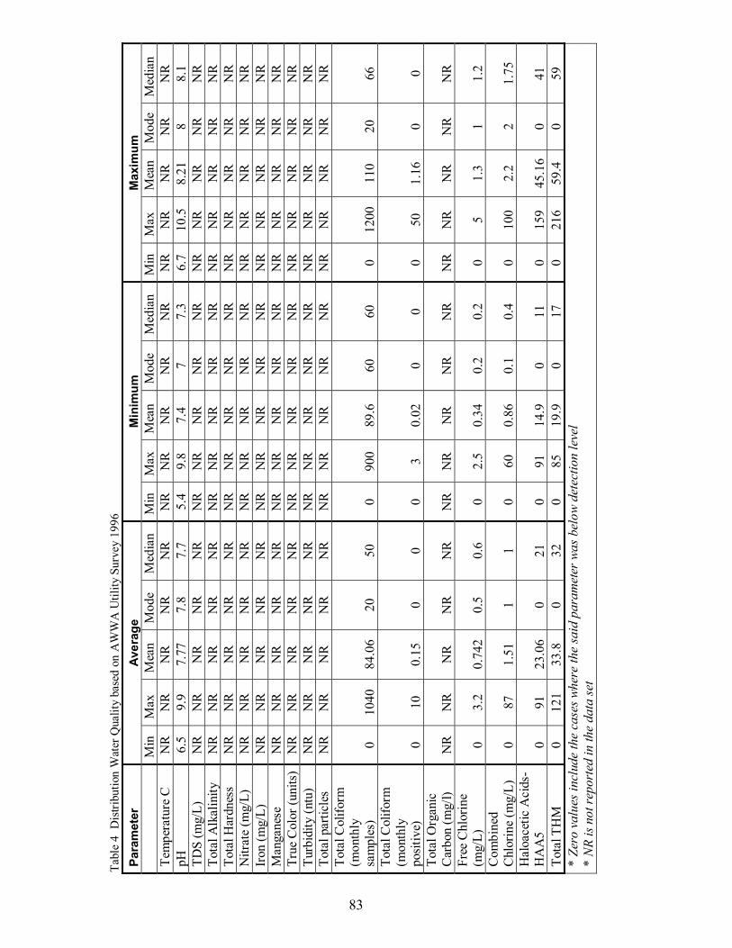
Tabl
e 4
Dis
tribu
tion
Wat
er Q
ualit
y ba
sed
on A
WW
A U
tility
Sur
vey
1996
Pa
ram
eter
Av
erag
e M
inim
um
Max
imum
Min
M
ax
Mea
n M
ode
Med
ian
Min
M
ax
Mea
n M
ode
Med
ian
Min
M
ax
Mea
n M
ode
Med
ian
Tem
pera
ture
C
NR
N
R
NR
N
R
NR
N
R
NR
N
R
NR
N
R
NR
N
R
NR
N
R
NR
pH
6.
5 9.
9 7.
77
7.8
7.7
5.4
9.8
7.4
7 7.
3 6.
7 10
.5
8.21
8
8.1
TDS
(mg/
L)
NR
N
R
NR
N
R
NR
N
R
NR
N
R
NR
N
R
NR
N
R
NR
N
R
NR
To
tal A
lkal
inity
N
R
NR
N
R
NR
N
R
NR
N
R
NR
N
R
NR
N
R
NR
N
R
NR
N
R
Tota
l Har
dnes
s N
R
NR
N
R
NR
N
R
NR
N
R
NR
N
R
NR
N
R
NR
N
R
NR
N
R
Nitr
ate
(mg/
L)
NR
N
R
NR
N
R
NR
N
R
NR
N
R
NR
N
R
NR
N
R
NR
N
R
NR
Ir
on (m
g/L)
N
R
NR
N
R
NR
N
R
NR
N
R
NR
N
R
NR
N
R
NR
N
R
NR
N
R
Man
gane
se
NR
N
R
NR
N
R
NR
N
R
NR
N
R
NR
N
R
NR
N
R
NR
N
R
NR
Tr
ue C
olor
(uni
ts)
NR
N
R
NR
N
R
NR
N
R
NR
N
R
NR
N
R
NR
N
R
NR
N
R
NR
Tu
rbid
ity (n
tu)
NR
N
R
NR
N
R
NR
N
R
NR
N
R
NR
N
R
NR
N
R
NR
N
R
NR
To
tal p
artic
les
NR
N
R
NR
N
R
NR
N
R
NR
N
R
NR
N
R
NR
N
R
NR
N
R
NR
To
tal C
olifo
rm
(mon
thly
sa
mpl
es)
0 10
40
84.0
6 20
50
0
900
89.6
60
60
0
1200
11
0 20
66
To
tal C
olifo
rm
(mon
thly
po
sitiv
e)
0 10
0.
15
0 0
0 3
0.02
0
0 0
50
1.16
0
0 To
tal O
rgan
ic
Car
bon
(mg/
l) N
R
NR
N
R
NR
N
R
NR
N
R
NR
N
R
NR
N
R
NR
N
R
NR
N
R
Free
Chl
orin
e (m
g/L)
0
3.2
0.74
2 0.
5 0.
6 0
2.5
0.34
0.
2 0.
2 0
5 1.
3 1
1.2
Com
bine
d C
hlor
ine
(mg/
L)
0 87
1.
51
1 1
0 60
0.
86
0.1
0.4
0 10
0 2.
2 2
1.75
H
aloa
cetic
Aci
ds-
HA
A5
0 91
23
.06
0 21
0
91
14.9
0
11
0 15
9 45
.16
0 41
To
tal T
HM
0
121
33.8
0
32
0 85
19
.9
0 17
0
216
59.4
0
59
* Ze
ro v
alue
s inc
lude
the
case
s whe
re th
e sa
id p
aram
eter
was
bel
ow d
etec
tion
leve
l *
NR
is no
t rep
orte
d in
the
data
set
83
84
Table 2 and Table 3 present the summary of the finished water quality for ground
water and surface water utilities respectively. Even if modal values are considered, the
parameters in Table 2 and Table 3 show a fair degree of variability. The summary of the
water quality parameters in distribution system is given in Table 4. The variability in
values of pH, Chlorine, total hardness, total alkalinity, total dissolved solids and turbidity
in Table 2 through 4 is of interest, as discussed later in the chapter these parameters have
a dominant role in copper pitting.
Interestingly, the maximum of the average values for finished water for certain
parameters in Table 2 and Table 3, exceed the maximum limit suggested by USEPA
secondary standards. These parameters include pH, total dissolved solids, iron and
manganese. Similarly, the maximum of the average concentrations for free chlorine and
combined chlorine are about 6~7 mg/ L for finished water, which is above the maximum
residual disinfectant level (MRDL) of 4.0 mg/ L as mandated by USEPA primary
standards. The maximum of the average nitrate concentrations for both ground and
surface water exceed the maximum contaminant limit (MCL) of 10 mg/L as mandated by
USEPA primary standards. The reason for deviation from primary standards by these
utilities is not explained in the data. A possible explanation may be because the data
pertains to 1996 whereas the Disinfection / Disinfection byproduct rule-I was
promulgated in 1998.
Some of the parameters like Sulfate, Carbon Dioxide, and Dissolved Oxygen are
not reported in the database, it is very likely that these parameters were not measured.
85
These parameters have been very often identified as the principal causes for copper
failures, although, their absence does not guarantee non occurrence of pitting. The
database does not provide anionic breakdown for parameters like hardness, alkalinity,
total dissolved solids, and turbidity, hence conclusions regarding pitting susceptibility of
houses in specific utilities could not be made. Most of the parameters for distribution
system water quality (Table 4) are either not measured or not reported in the database,
thus the variability between the quality of finished water and quality of water in
distribution system could not be assessed directly.
In summary the analysis suggests that the water quality parameters have fair degree
of variability across different utilities and also within the distribution system. The
variability in pH, chlorine, total hardness, total alkalinity, total dissolved solids and
turbidity in finished water and in distribution system is of interest. Due to absence of
complete anionic breakdown an objective comparison between the finished water quality
and the distribution system water quality is difficult. Certain other parameters like,
Dissolved Oxygen and Carbon Dioxide are not reported in the database. Based on the
above data, the factors affecting the copper pitting are discussed with respect to the
present literature.
Factors affecting copper pitting
The following text is based upon a review of a number of sources concerning copper
corrosion. Since we did not conduct any experiments or studies, mechanisms or details
as published by other sources are only reported and summarized herein, and these authors

86
are not validating or confirming their conclusions. All attempts have been made to
represent the current understanding of copper plumbing corrosion as accurately as
possible. The factors that influence copper pitting may be broadly classified into two
categories, namely physical and chemical parameters. Most of the corrosion problems are
due to the complex synergy between these parameters (Schock, 1999). In general most of
these parameters are dictated by the parameters of the major distribution system, where
the variability in these parameters is much larger as compared to the variability of these
parameters within the home plumbing system. A detailed discussion on the effect of these
parameters is presented.
Physical parameters
The physical parameters include pressure, velocity, temperature and
anthropogenic effects. While the pressure and velocity are proportional, certain devices
such as valves, low flow faucets can affect the flow and hence the velocities.
Temperature becomes a variable, when we consider cold water pipes, hot water pipes and
hot water recirculation system. Many aspects of water chemistry like ionic dissociation
and degasification of gases are related to temperature and pressure of water.
Anthropogenic effects include poor workmanship, improper design, improper flushing
after installation etc. The physical parameters and their effects are discussed in detail.
Pressure and Velocity
All home plumbing systems are pressurized systems. The pressure ( ip ) and
velocity ( iv ) in any pipe in home plumbing system are highly dependent on the street
87
level pressure ( streetP ). The street level pressure is the pressure measured in the street
lateral that connects to the home plumbing system with a service line. Thus hydraulically,
the street level pressure becomes a boundary condition for the home plumbing system. If
the effects due to transience and compressibility are ignored, then the street level pressure
( streetP ) can be expressed in terms of pressure ( ip ), velocity ( iv ) and elevation ( ih ) of
any pipe using the energy equation.
water
streetLossesi
i
water
i PHh
gvp
γγ=+++
2
2
(1)
Where,
ip is the pressure in any pipe ( i ) in home plumbing system
iv is the velocity in pipe ( i )
ih is the difference in elevation between the street lateral and the point of measurement
g is the acceleration due gravity
waterγ is the unit weight of water (considering constant density)
LossesH is the sum of minor and friction losses from the street lateral to the point of
measurement
Hence, any change in the street level pressure ( streetP ) would affect the velocity
and pressure in the home plumbing system. Thus the street level pressure ( streetP ) defines
the boundary condition for any home plumbing system. Interestingly, the street level

88
pressure is subjected to change with positioning of the house with respect to the pumping
station. There may be high pressure and low pressure zones within the big distribution
system, the behavior of a plumbing system in these zones would be markedly different
from one another due to the change in the boundary condition. Additionally, the street
level pressure may drop significantly during peak hours due to simultaneous withdrawal,
causing much lower velocities ( iv ) and pressure ( ip ) as compared to the velocities and
pressure in the non peak hours. The complexities and the variations of street level
pressure itself is a subject of research.
The phenomenon of erosion corrosion is associated with higher flow rates. Due to
impingement of water on the pipe wall the protective coating or the scale on the pipe wall
gets damaged mechanically. This causes non uniform wearing of pipe wall locally,
eventually causing a leak. A combination of high velocities, low pH and high DIC
(dissolved inorganic copper) is extremely aggressive towards copper (Schock, 1999).
Flow velocities ( iv ) above 4~6 feet per second or pressure ( ip ) above 80 psi are
considered high (CDA reports). In general, the desirable velocity in plumbing system is
between 4 and 6 feet per second (Woodson, 2002). Although, the threshold values of
pressure ( ip ) and velocity ( iv ) which may cause pinhole formation are difficult to
establish. In general, the threshold values will depend on several parameters including
pipe diameter, water chemistry, flow constrictions, extent of faucet opening, presence of
scale etc. Hence, the values ascertained by CDA reports can be considered as
preliminary, the actual threshold values of pressure ( ip ) and velocity ( iv ) are not
available in present literature.

89
On the other hand, higher velocities may increase the diffusion rates of protective
species within the pipe, thereby helping in preventing corrosion (Schock, 1999). For
instance, the formation of protective oxide film is dependant on the transport rate of
dissolved oxygen, which is limited by the flow velocity. This can be mathematically
modeled by assuming the pipe to behave like a plug flow reactor, and first order decay
for oxygen in bulk solution,
0).(),()(),( =+∂
∂+∂
∂ txkcx
txctut
txc (2)
Where,
),( txc is the concentration of any protecting species at a time t and distance .x
)(tu is the flow velocity at time t .
k is the first order decay constant for the species in bulk solution.
However, in general the higher velocities are considered deleterious and should be
kept within reasonable range. The cause of higher velocities may be high street level
pressure or flow constrictions. The flow constrictions in the pipes may be due to sharp
bends where the flow separates from the pipe boundary or may be due to presence of
gaseous cavities at any cross section. These cavities are formed due to drop in pressure,
which decreases the solubility of gases. The solubility of any gas in water is dependent on
pressure and temperature hence the gases that are dissolved in water at higher pressure
tend to strip out of water at lower pressure, if temperature is considered constant. The
phenomenon can be explained considering water to be a homogenous two phased liquid.

90
The gases (oxygen, chlorine or other) are present in water in dissolved states.
Considering water as a bubbly homogeneous mixture of these gases, and using Henry’s
law,
0pp
SVV sg ≈ (3)
Where,
S is the solubility coefficient.
gV is the volume of dissolved gas.
V is the volume of water.
sp is the saturation pressure of the dissolved gas (absolute).
0p is the standard pressure (absolute).
The left hand term of Eqn (3) is the void ratio of the gas and is pressure
dependent. Hence, for any change in pressure the volume of dissolved gas should change
for a given volume of water. This gives rise to the degasification of water at low
pressures. It can be inferred that if the pressure is reduced to some other value p , then the
volume of gas evolved per unit volume of liquid is given by 0/)( pppS s − . The values
of S , are known for various gases at standard pressure conditions. If the release of gases
or the degasification is assumed a one way phenomenon, then these gases once released
should accumulate as isolated gaseous cavities at the highest elevation (being lighter than
water). These isolated gaseous cavities may either combine to form bigger cavities and
eventually reduce the net area of flow or these cavities may collapse at the pipe wall

91
creating high pressure. In former case, the result is the higher flow velocities at the cross
section which may cause erosion corrosion, while in later case, the effects may include
damages due to gaseous impingement or vibrations or rattling of pipes. Both these effects
may cause wear and tear at the pipe wall and in the protective scale. Velocity has been
found to contribute to aluminum catalyzed pitting of copper at high pH and in the
presence of chlorine. A recent masters’ thesis (Nguyen, 2005) determined that this type
of pitting did not occur if velocity was too low. Thus, there is a possibility that high
velocities are a necessary precondition for certain types of pitting attack, even if
excessive velocity alone is not the sole cause.
In summary, the effects of flow velocities and pressure are complex and may give
rise to multiple phenomenons that could cause wear and tear in the pipe. Excessive
velocities, high and low pressure should be checked to avoid problems related to gaseous
cavitation and erosion corrosion.
Temperature
Temperature plays a significant role in copper corrosion. The effects of
temperature are complex and are often misunderstood (Schock, 1999). The change in
temperature can affect solubility of solids, influence formation of complex ions, influence
diffusion rates of dissolved gases and solution species and influence formation of certain
scales on the copper surface. Sometimes, the changes in temperature influence multiple
phenomenons and hence make the situation complex (Schock, 1999). The solubility of
gases is decreased markedly by increase in temperature. Hence, in hot water pipes and

92
hot water recirculation systems, the degasification of the water can lead to formation of
gaseous cavities and hence increased velocities at certain cross sections leading to erosion
corrosion. This fact is supported by the anecdotal evidence in CDA reports, wherein
majority of failures in hot water pipes and hot water circulation system are due to erosion
corrosion. Due to entrapment of gases and continuous flow conditions, the erosion
corrosion is likely to affect hot water recirculation systems more than hot water pipes.
Due to increase in temperature, most of the gases are expected to be released in hot water
pipes and hot water recirculation system, hence water in these pipes is likely to have
lesser dissolved oxygen, therefore the mechanism like oxygen differential cell corrosion
and gaseous cavitation are less likely in these pipes as compared to cold water pipes.
However, the occasional occurrence of these mechanisms in hot water pipes and hot
water recirculation system is not ruled out.
The solubility of certain chemical species in water is also highly dependent on
temperature. The solubility of Calcium Carbonate [CaCO3] is decreased with increase in
temperature (Schock, 1999). Hence, at higher temperatures, Calcium Carbonate tends to
come out of water and form a scale on the pipe wall. The Calcium Carbonate scale is a
protective scale. Hence in hot water pipes and hot water recirculation systems
temperature may have beneficial effects with respect to scale formation. However,
excessive scale may sometime decrease the hydraulic conductivity of the water lines and
in the worst case may cause clogging of hot water lines.

93
The effects of temperature are also important with respect to pH changes, these
effects are illustrated further. The dissolved inorganic carbon (DIC) is defined as a
function of Carbonate species [CO32-], Bicarbonate species [HCO3
-] and [H2CO3*]
Carbon dioxide gas and Carbonic acid molecules (Schock, 1999).
DIC= [H2CO3*] + [HCO3-] + [CO3
2-] (4)
Where,
[CO32-] is the concentration of Carbonate species in mol/ L
[HCO3-] is the concentration of Bicarbonate species in mol/ L
[H2CO3*] is the sum of dissolved Carbon dioxide and Carbonic acid molecules.
The increase in temperature increases the dissociation constant for water, thereby
producing more H+ and OH- ions, which tends to decrease the pH of water, however, this
phenomenon is accompanied by increase in dissociation of Carbonic acid [H2CO3], which
increases H+ and HCO3- ions in water, the Bicarbonate ions [HCO3
-] provide buffer
against change in pH. However, due to deposition of Calcium Carbonate scale, the DIC is
reduced, thereby reducing the buffering effect provided by the Bicarbonate ions. For
waters with low alkalinity (< 50 mg/L of CaCO3), the overall effect may be reduction of
pH at higher temperatures (Schock, 1999). Thus high temperatures in water with low
alkalinity may bring down the pH of water significantly.
94
The role of temperature is also important with respect to the type of scale that
forms on the copper surface. Edwards et al. (1994) state that brochantite
[Cu4(OH)6(SO4)], a scale that supposedly catalyses pitting, is more stable at higher
temperatures. Also, malachite [Cu2(OH)2CO3], a protective scale is comparative less
stable at these temperature ranges. The higher frequencies of failures in hot water pipes is
due to the formation of brochantite [Cu4(OH)6(SO4)] where temperatures are much higher
and closer to 100o C (Edwards et al. 1994).
Overall, the effects of temperature are complex and may be deleterious to copper
in both cold and hot water pipes. However, these effects are highly subjective to water
chemistry like pH, alkalinity and concentration of other anions. For instance, the
brochantite scale may not form in hot water with higher pH, since the solubility of
brochantite is increased at higher pH (> 7.4), also the increase in concentration of
bicarbonate at a lower pH (<7.4) may result in formation of malachite scale. Hence, the
effect of increase in temperature is highly subjective to water chemistry.
Anthropogenic effects
These effects include the factors that are introduced due to human errors in the
process of commissioning or installation of the home plumbing systems. The effects also
include poor practices during or after the installation that can induce copper pitting. Poor
workmanship is perhaps the most important cause and can induce pitting failures in less
than a year of installation. The CDA reports define poor workmanship as improper
cutting of pipes (pipes that are not squarely cut and not reamed), excessive soldering flux

95
and improper joining of pipes. Poor workmanship may be a result of accelerated
construction period, human negligence or under qualified plumbing technicians deployed
during the installation. This category of failures is categorized as soldering flux induced
failures in CDA reports. Soldering flux induced failures may be avoided by ensuring that
the plumbing technicians use the industry standard material and practices when installing
copper tube systems (Myers and Cohen, 2005). The fluxes should comply with ASTM
B813 and soldering connections should be made in accordance to ASTM B 828 (Myers
and Cohen, 2005). Ellis II, (2000) elaborates that excessive soldering flux reacts with
cupric oxide to produce hydrochloric acid, which increases the rate of pitting by
supplying chloride ions. Flux induced leaks, once started are difficult to stop, typically it
requires re plumb after four or five leaks (Myers and Cohen, 2005).
In addition to the poor installation practices, sometimes post construction
activities can cause pitting in home plumbing systems. If the copper pipes are not flushed
properly, the debris accumulated at the bottom of the horizontal pipes may induce pitting
due to oxygen differential mechanism (Rossum 1985). Long stagnation periods between
installation and usage, may cause complete decay of the residual disinfectant which may
induce copper pitting due microbiological growth. The period between the installation
(when the water enters the copper pipes) and usage should not exceed two months
(Rossum 1985).
All the above cited reasons are more of practical nature and are directly related to
the practices during and after installation. To certain extent the above reasons are of

96
human control and are a matter of embracing certain practices that can save pitting
problems due to the aforesaid reasons.
Chemical parameters
Most of the theory and practical experiences suggest that the causes of pitting
revolve around water chemistry. The nature of certain anion species (Chloride and
Sulfate) seems to show variable character in different water chemistries. Some
researchers have identified the role of pH and dissolved carbon dioxide as the dominating
factor in copper pitting. However, there is no direct correlation of carbon dioxide
concentration and its role in any corrosion mechanism (Schock, 1999). The nature of
interaction of any anionic species in water with the copper is highly subjective to pH and
pressure conditions. The review of chemical parameters affecting copper pitting is
presented with respect to copper chemistry.
Review of Copper Chemistry
Copper metal is oxidized to the cuprous (+1) and cupric (+2) oxidation states in
corrosion. Under strong oxidizing conditions, higher oxidation states of (+3) and (+4) for
copper are also known but those are not important in plumbing corrosion (AWWA 1996).
When copper corrodes to (+1) or (+2) oxidation states, it may form insoluble precipitates
or soluble complexes. The soluble complexes contribute to copper concentrations in
drinking water. The precipitates may form passivating film, cuprite [Cu2O] or cupric
species [CuO] or may be present in water in form of blue or green turbid suspensions.
The formation of such scale (cuprite or cupric) plays a key role in reducing the rate of the

97
corrosion (Edwards et al. 1994). The type of scale that forms on the copper surface is
highly dependant on water chemistry. The type of scale not only depends on the anions
present in water, but it also depends on other conditions like their relative concentration,
pH and temperature. The common anions that may form solid scales are chloride, sulfate,
nitrate and bicarbonate (Edwards et al. 1994). The scale thus formed may be soluble or
precipitate as solids depending upon the pH and temperature of the water. Based on the
Pourbaix diagram of copper, it can be inferred that the cuprite [Cu2O] is stable on a
narrow range of pE values, and tenorite [CuO] is stable at alkaline pH values for water at
equilibrium with atmospheric oxygen (AWWA 1996).
Thus, in drinking water pipes it is hypothesized that the copper oxidizes to
cuprous (+1) state by losing an electron in the first step, this process is facilitated by the
electron acceptor species; generally aqueous chlorine ,dissolve oxygen or hydrogen ion.
The anodic reaction is given by,
−+ +→ eCuCu metal )( (5)
++ +→+ HOCuOHCu solid 22 )(22 (6)
Cuprite [Cu2O], often known as cuprous oxide is brownish red and is often found
as thin and continuous film on the pipe wall. Cuprite, being stable in a narrow range of
pE, may be further oxidized to tenorite [CuO] at alkaline pH values in the second step.
The reactions require an electron acceptor, which is generally aqueous chlorine, dissolved

98
oxygen or hydrogen ions. Tenorite [CuO] is black in color and is more stable in alkaline
pH range. The anodic reaction is given by,
−−+ ++→+ eOHCuOHOCu solid2
2)(2 21
21 (7)
++ +→+ HCuOOHCu solid 2)(22 (8)
The corresponding cathodic reaction for both the steps may occur in three
possible ways. If the water contains aqueous chlorine, it shall dominantly participate in
the cathodic reaction as compared to hydrogen ions or dissolved oxygen; this is because
chlorine has high electron affinity. The reaction takes place in two steps; the first step
involves dissolution of gaseous chlorine in water forming Hypochlorous acid [HOCl].
The Hypochlorous acid ionizes in the second step, yielding hydrogen ion [H+] and
hypochlorite ion [OCl-] (Viessman, 1993). The equations are given by,
−+ ++⇔+ ClHHOClOHCl 22 (9)
+− +⇔ HOClHOCl (10)
The dissociation of Hypochlorous acid [HOCl] to hypochlorite ion [OCl-] is rapid, so that
equilibrium is maintained even if the former is being continuously consumed. At pH
around 7.5, both the species [HOCl] and [OCl-] occur almost in equal concentration
(Viessman, 1993). At higher pH values (> 7.5) the dissociation rate of Hypochlorous acid
increases, due to which Hypochlorite ion exists in abundance as compared to

99
Hypochlorous acid. The phenomenon is completely reversed at lower pH values (< 7.5 ).
Hence, at lower pH values (<7.5), Hypochlorous acid [HOCl] becomes the dominant
species that accepts electrons and facilitates cathodic reaction and at higher pH values (>
7.5), Hypochlorite ions [OCl-] facilitates the cathodic reaction. The corresponding
equations are given by,
For pH < 7.5
OHCleHHOCl 22 +→++ −−+ (11)
For pH > 7.5
OHCleHOCl 222 +→++ −−+− (12)
In case free chlorine is not present, the cathodic reaction is facilitated by reduction of
dissolved oxygen, the reaction is given by
−− ⇔++ OHeOHO 442 22 (13)
If even dissolved oxygen is not present, the cathodic reaction is facilitated by reduction of
hydrogen ion to hydrogen. The reaction is given by

100
222 HeH ⇔+ −+ (14)
Irrespective of which reaction takes place at cathode, there is an increase in pH either due
to consumption of hydrogen ions or due to production of hydroxyl ions. This drop in pH
is localized and is different than the pH in bulk solution (Schock, 1999).
Another form of copper scale commonly found is copper carbonate or malachite
[Cu2(OH)2CO3]. Edwards et al. (1994), state that over a pH range of 5.5~9.5, tenorite
[CuO] and malachite [Cu2(OH)2CO3] are predicted to be dominant cupric solids. The
presence of either of these solids depends on the bicarbonate concentration and the pH of
water. For pH below 7.7 and high bicarbonate concentrations, malachite [Cu2(OH)2CO3]
is favored, whereas for higher pH values and high bicarbonate concentrations tenorite
[CuO] is favored. For low bicarbonate concentrations, tenorite [CuO] is favored at all pH
values above 6.5. Edwards et al. (1994) illustrate that the solubility of the tenorite [CuO]
is increased at higher bicarbonate concentrations, hence water with high pH and high
bicarbonate concentration is not expected to form a malachite [Cu2(OH)2CO3] scale,
additionally it would increase the solubility of the protective tenorite [CuO] film.
Since, the solubility of other copper solids like copper hydroxide, copper chloride,
cupric nitrate is more than malachite [Cu2(OH)2CO3] and tenorite [CuO], their presence
on the scale in plumbing systems is very unlikely (Edwards et al. 1994). The other copper
salt that is commonly present on pipe surface is brochantite [Cu4(OH)6(SO4)], due to
better stability at higher temperature, it is commonly found in hot water pipes or hot
101
water recirculation system (Edwards et al.1994). However, the formation of the
brochantite is subjective to the concentration of bicarbonates and pH conditions. Hence,
for waters with high sulfate to bicarbonate ratio, pitting is likely in hot waters due to the
formation of brochantite. In cold water pipes, the formation of brochantite formation is
favored at high sulfate to bicarbonate ratio and high sulfate to chloride ratio. Brochantite
formation is like to increase pitting in the waters that have undergone softening (Edwards
et al. 1994).
To summarize, the formation of scale on the pipe surface is highly dependent on water
chemistry, relative concentration of anions, alkalinity, temperature, pH etc. The scale thus
formed may be protective or non protective depending upon the water chemistry. The
most common scales that can form in copper water pipes are malachite [Cu2(OH)2CO3],
tenorite [CuO] and brochantite [Cu4(OH)6(SO4)], other copper solids formed are
generally soluble at the pH range of interest.
The following section elaborates the role of water quality parameters that can
influence copper pitting. The influence of all the known parameters is discussed in detail.
The role of some of the chemical parameters like, pH, total alkalinity (TALK), dissolved
inorganic carbon (DIC), hardness, total dissolved solids (TDS), dissolved oxygen and
corrosion inhibitors is presented in the following section. The role of other parameters,
namely, nitrate, chloride, chlorine, chloramines, hydrogen sulfide, sulfate, Iron, zinc,
manganese, aluminum and natural organic matter (NOM) is described in Appendix B-2.
102
pH
pH is a measure of the activity of hydrogen ions, H+, present in water (Schock,
1999). For pure water the pH value is 7, which is considered as a value for neutral
solutions. For acidic conditions pH ranged between 1 and 7, while for basic solutions the
pH ranges between 7 and 14. Due to the presence of other species in potable waters the
pH is generally not neutral. During corrosion, the metal corrodes and losses electrons, in
order to facilitate this reaction the H+ ions accept electrons (Schock, 1999). For pitting
corrosion, pH is an important parameter, in the absence of protecting film, pitting is
likely to occur between pH 5 and 9 (Schock, 1999). If pH is too low, uniform corrosion is
expected (Edwards et al.1994). Uniform corrosion rapidly increases with decrease in pH,
it is significant in acidic waters (pH< 6), and may cause high soluble copper
concentrations (> 1.3 mg/L) without the evidence of “green or blue” water (AWWA
1996). At higher pH (> 7), the rate of the uniform corrosion is very small, mostly at pH
exceeding 7, the copper corrosion is considered to be non uniform (AWWA 1996).
pH is also important in formation of scales on pipe walls (Edwards et al.1994). As
discussed earlier with respect to copper chemistry, the role of pH is crucial for tenorite
[CuO] and malachite [Cu2(OH)2CO3] formation, as these scales are considered protective
to copper. For pH below 7.7 and high bicarbonate concentrations, malachite
[Cu2(OH)2CO3] is favored, whereas for higher pH values and high bicarbonate
concentrations tenorite [CuO] is favored. For low bicarbonate concentrations, tenorite
[CuO] is favored at all pH values above 6.5 (Edwards et al. 1994).

103
Edwards et al. (1994) illustrate that the solubility of the tenorite [CuO] is
increased at higher bicarbonate concentrations, hence water with high pH is not expected
to form a malachite [Cu2(OH)2CO3] scale, additionally it would increase the solubility of
the protective tenorite [CuO] film if it has higher bicarbonate concentrations. The role of
pH also affects the behavior of Sulfate [SO42-] and Chloride [Cl-] ions, a detailed
discussion on the role of pH for these anionic species is provided later when these species
are discussed. The adjustment of pH is usually done at the treatment plant as a part of
corrosion control measure (Schock, 1999). pH control is also used for balancing certain
chemical reactions (Maryland Task Force, 2004). The optimal pH required to prevent
corrosion depends on several factors including the pipe material in distribution system,
however, corrosion inhibitors like Orthophosphates require a narrow pH range for
maximum effectiveness (Schock, 1999). The pH is generally brought at or above neutral
levels (pH ≥ 7), by injecting chemicals such as Calcium Oxide or quick lime [CaO],
Calcium Bicarbonate [Ca (HCO3)2], hydrated lime [Ca (OH)2], or soda ash [Na2CO3] in
finished water (Maryland Task Force, 2004).
Altogether, pH plays a dominant role not only in dictating the type of corrosion
but also in formation or dissolution of certain scales that are important for copper pitting.
The measures to adjust the pH in the treatment plants depends on various factors
including the pipe material in the distribution system, nevertheless it is one of the reasons
of large variability in pH across various utilities.
104
From AWWARF utility survey, presented earlier, it is evident that the finished
water has considerable variation in pH values. The pH ranges between 5.5 to 10 for
finished ground waters and 5.4 to 10.6 for finished surface waters. The pH in distribution
system is also in similar range.
Alkalinity and DIC (dissolved Inorganic Carbon)
Alkalinity is a measure of the ability of water to neutralize acids and bases
(Schock, 1999). The dissolved inorganic carbon (DIC) is defined as a function of
Carbonate species [CO32-], Bicarbonate species [HCO3
-] and [H2CO3*] Carbon dioxide
gas and Carbonic acid molecules (Schock, 1999). Hence, mathematically,
DIC= [H2CO3*] + [HCO3-] + [CO3
2-] (4-rewritten)
TALK = 2[CO32-] + [HCO3
-] + [OH-] - [H+] (15)
Where,
DIC is expressed in mg C/L
[CO32-] is the concentration of Carbonate species in mol/ L
[HCO3-] is the concentration of Bicarbonate species in mol/ L
[H2CO3*] is the sum of dissolved Carbon dioxide and Carbonic acid molecules.
[OH-] is the concentration of hydroxyl ions in mol/ L.
[H+] is the concentration of hydrogen ions in mol/ L.
TALK is total alkalinity in equivalents/ L.
105
The dissolved inorganic carbon (DIC) has carbon dioxide as one of its component
(Eqn 4). The role of carbon dioxide in copper corrosion is in “considerable disagreement”
(AWWA, 1996). Although, some researchers have identified carbon dioxide as the major
culprit that causes copper pitting in presence of dissolved oxygen. In many of the CDA
reports, carbon dioxide concentrations exceeding 25 mg/ L in presence of dissolved
oxygen is associated with copper failures. The higher the dissolved concentration of
carbon dioxide, the greater the potential of pitting related to cold water (Myers and
Cohen, 2005; Cohen and Myers, 1984). Myers and Cohen, (2005), illustrate that the
concentration of the dissolved carbon dioxide can be lowered by increasing the pH, by
the following relationship.
)(05.0)()88.0( 2COLogpHTALKLogKILog =−++÷ (16)
Where
)88.0( KILog ÷ is the temperature factor, which is 6.35 at 55F.
Sobue et al. (2003) presented a possible correlation between the carbon dioxide
and copper pitting. The authors of the paper have themselves shown reservations towards
the hypothesis, and have expressed the need of further investigation. The possible
reactions presented by Sobue et al. (2003) are,
106
)(2)(2 aqg COCO → (17)
322)(2 COHOHCO aq →+ (18)
+− +→ HHCOHCO 33 (19)
The authors of the paper have further suggested that the last step (Eqn 19) may possibly
facilitate reduction of oxygen at cathode by supplying the hydrogen ion.
OHeHO 22 244 →++ −+ (20)
Since, the reduction of oxygen, is coupled with oxidation of copper at anode, the reaction
will precede causing corrosion of copper. Nevertheless, the role of carbon dioxide
remains unclear.
From Eqns (4) and (15), it is clear that there is a strong relationship between DIC
and TALK. The concentration of Bicarbonate and Carbonate ions is directly related to pH
of water (Schock, 1999). For a given pH and temperature, total alkalinity and DIC follow
a straight line relationship. The slope of the line increases with increase in pH. Hence, for
a given pH and temperature, an increase in DIC will increase the total alkalinity, while
for a given DIC concentration and temperature a reduction in pH will cause a reduction in
total alkalinity (Schock, 1999). The total alkalinity is usually expressed in mg CaCO3/ L,
it is calculated by alkalinity titration as carbonic acid equivalence point. When bases
other than CO32-, HCO3
- and OH- are present in water, the definition of the total alkalinity
should include the concentration of all proton consuming species, with proper corrections

107
for their respective dissociations (Schock, 1999). Schock, (1999) defines a general
equation for total alkalinity, in waters containing orthophosphate, hypochlorite, ammonia,
silica, and some singly charged organic species as,
TALK = 2[CO32-]+[HCO3
-]+[OCl-]+[HPO42-]
+[OA-] +[NH3]+[H3SiO4-]+[OH-]-[H+] (21)
Where,
[OCL-] is the concentration of hypochlorite in mol/ L.
[HPO42-] is the concentration of orthophosphate in mol/ L.
[OA-] is the concentration of singly charged organic species in mol/ L
[NH3] is the concentration of ammonia in mol/ L
[H3SiO4-] is the concentration of silicate in mol/ L
The above equation is based on the assumption that the concentrations of species
like PO43- and H2SiO4
2- will be low due to small dissociation constants in the normal
potable waters. The dissociation constants for these species increase markedly with
increase in pH, thereby supporting the notion that increase in pH leads to increase in total
alkalinity. Some of these species (orthophosphate and silicates) are used as corrosion
inhibitors it is possibly due to this reason that pH adjustment becomes almost a necessary
measure at the treatment plant. The increase in pH not only increases the dissociation of
these species but it also strips carbon dioxide from water. As stated earlier, while
108
adjusting the pH in the treatment, the alkalinity of the water is increased by increasing the
carbonate, bicarbonate and hydroxyl species.
As discussed in copper chemistry, the oxidation of copper is facilitated by
electron accepting species at cathode. The cathodic reaction is facilitated by the reduction
of either hypochlorite [OCl-], hypochlorous acid [HOCL] or hydrogen ion [H+]. refer
Eqn (11) ~(14). And, the reaction at cathode is followed by a localized reduction in pH,
which is different than pH in bulk solution (Schock, 1999). The rate of the cathodic
reaction may be affected if the water resists such a change in pH. The ability of the water
to resist such a change in pH is defined as its buffer intensity. Importantly, the DIC
(dissolved inorganic carbon) plays a key role in providing buffer against the pH changes.
The buffer intensity of water against an increase or decrease in pH is a function of
alkalinity, DIC concentration, and pH of water (Schock, 1999). An increase in DIC
provides higher buffer intensity to water for all pH ranges. For a particular DIC
concentration, the buffer intensity changes with pH, the behavior is almost sinusoidal.
The buffer intensity is maximum at about pH~7, any increase in pH decreases the buffer
intensity and brings it to a minimum at about pH~ 8, higher values of pH causes an
increase in buffer intensity. Interestingly, by increasing the alkalinity, the behavior of the
buffer intensity does not change, additions of corrosion inhibiting species like
orthophosphate, silicate does not increase the buffering ability of water at pH values till ~
9 (Schock, 1999). Thus the carbonate and the bicarbonate system are primarily
responsible for providing buffer.
109
This concludes that addition of carbonates and bicarbonates may provide
beneficial effects at certain pH ranges with respect to buffer intensity, while at pH closer
to ~8, the buffering effect of the carbonates and the bicarbonates is minimal and hence
adding these species to water may not yield any substantive gain in terms buffering
effects at the said pH range. Also, the addition of bicarbonate is generally believed to
have beneficial effects and an increase in bicarbonate concentration increases the
likelihood of formation of passivating scales (Edwards et al. 1994).
The AWWARF/ AWWA utility survey data presented earlier provides the range
for alkalinity values (Table 2 & 3) for finished ground and surface waters, respectively.
The total alkalinity for finished ground waters ranges between 0 and 510 mg/ L of
CaCO3. The total alkalinity range for surface waters is 0 to 700 mg/ L of CaCO3. The
breakdown of the anionic species that constitutes the total alkalinity values is not
provided, hence, any conclusions could not be made regarding the dissolved inorganic
carbon (DIC) and the buffer intensities of these waters.
Hardness and TDS (total dissolved solids)
Hardness is defined as the sum of Calcium [Ca2+] and Magnesium [Mg2+]
concentrations and is expressed in equivalents of CaCO3 (Tchobanoglous, 1985). The
hardness can be further classified into carbonate hardness and non carbonate hardness.
The carbonate hardness is associated with bicarbonate [HCO3-] and carbonate [CO3
2-]
species of magnesium and calcium, while non carbonate hardness is associated with other
anions, mainly, chloride [Cl-] and sulfate [SO42-]. The type of hardness is extremely

110
important from the perspective of scale formation. The formation of scale is highly
dependant on the concentration of calcium carbonate in bulk solution.
Hence, waters with high carbonate hardness (and low non carbonate hardness),
will have more carbonates and bicarbonates in bulk solutions, and hence more likely to
form carbonate scale. Since, the alkalinity of water is dependent on carbonate and
bicarbonate concentrations, such waters will have more alkalinity. On the other hand,
hard waters with more non carbonate hardness (and less carbonate hardness), will have
more sulfate or chloride anions as compared to carbonate and bicarbonate ions in the bulk
solution. These waters are therefore less likely to form carbonate scale. Since, these
waters have less carbonate and bicarbonate in bulk solution; they are lower in alkalinity
as compared to the former case.
Hard waters are in general are less corrosive than soft waters, if sufficient
alkalinity is present (Schock, 1999). The stress on alkalinity necessarily illustrates the
type of hardness (carbonate or non carbonate) as explained above. The effects of
temperature are important with respect to alkalinity. For instance, at high temperatures (in
hot water pipe or hot water recirculation systems), the calcium carbonate scale is formed
due to decrease in solubility of calcium carbonate. The scale thus formed is protective
and hence beneficial from pitting perspective. In coldwater pipes, in general, the calcium
carbonate scale does not form, exceptions to this rule may be found in systems where
water is softened with lime or soda lime by making the water super saturated with

111
Calcium carbonate (Schock, 1999). The above discussion has led us to the definition of
Type-I pitting.
Type I pitting is likely to occur in hard, cold, well waters with high sulfate
concentration relative to chloride and bicarbonate and with high carbon dioxide in
between pH 7~ 7.8 (Edwards et al. 1994). The conditions defined for Type-I pitting may
be explained with respect to the previous discussion. If water has high sulfates relative to
bicarbonates and chlorides, it follows that it is low in alkalinity, also almost all the
hardness present in the water is sulfate (non carbonate hardness), now since the water is
cold, the calcium carbonate scale should not form (as water is low in carbonates), hence
leaving the surface of pipe exposed to sulfate anions that cause corrosion. The role of
carbon dioxide is not clearly explained in the publication. The most likely explanation
can be attributed to the increase in conductivity of the solution due to dissociation of
carbonic acid, as explained in Eqn (18). This type of pitting is generally associated with
cold water pipes; however, their occasional occurrence in hot waters is also reported
(Edwards et al. 1994).
The reason of the occurrence of Type-I pitting in hot waters is attributed to the
lack of comprehensive theory with respect to water quality (Edwards et al. 1994).
However, this can be explained on the lines of above discussion. With increase in
temperature, the solubility of the calcium carbonate should decrease and it would be
expected that the calcium carbonate scale will form, however, another phenomenon
dominates. Since, the water is low in carbonates and bicarbonates, it necessarily has

112
lower DIC (dissolved inorganic carbon) and low alkalinity, because of lower DIC the
water has poor buffer intensity against pH changes. In hot water pipes or hot water
recirculation systems, initially, the higher temperatures cause a decrease in solubility of
calcium carbonate, however, the net effect due to higher temperatures and low alkalinity
is the reduction in pH (Schock, 1999). The decrease in pH increases the solubility of
calcium carbonate thus preventing the scale formation, and leaving the pipe surface
exposed to sulfate ions. It follows from the above discussion that alkalinity plays a
significant role in Type-I pitting.
Type-II pitting may occur in hot water pipes with low pH (< 7.2) and high sulfate
concentration relative to bicarbonate, with occasion deposits of manganese (Edwards et
al. 1994). The possible explanation to this type of pitting is as follows. Since, there is no
mention about the amount of calcium carbonate in the water, two possibilities arise. One,
water has significant calcium carbonate almost equal to or nearly saturation level. Two,
the calcium carbonate content in water is significantly low. The explanation for both
these cases is presented. Since the pH and the bicarbonate concentration are low, the
alkalinity of the water is determined by the concentration of carbonates (present as
calcium carbonate). If the concentration of calcium carbonate is significant, then water
would be highly alkaline and moderate DIC level. In hot water pipes, the likelihood of
calcium carbonate scale formation is fairly high, as the DIC provides a buffer against the
change in pH and the rise in temperature decreases the solubility of calcium carbonate
without affecting the pH. Under these conditions the pitting is not likely. However, if the
calcium carbonate concentration is low, then due to lower DIC the said water has poor

113
buffer intensity against the pH change. With increase in temperature, there will be a
further drop in pH which further increases the solubility of calcium carbonate. The
calcium carbonate scale will not form. Hence, pitting is very likely. Importantly, from the
above explanation, this type of pitting can also occur in cold water pipes, since calcium
carbonate scale formation is less likely (carbonate is present in low concentration). The
role of manganese in Type-II pitting is not very clear. There have been instances when
hot water pitting is observed without manganese deposits (Edwards et al. 1994).
Nevertheless, the type of hardness is important from copper pitting perspective, if
the hardness is present as carbonate hardness, then it may have some beneficial effects
with respect to alkalinity and DIC, however, if the hardness is non carbonate hardness
then water will have lower DIC and less buffer. The role of sulfate and chloride will be
explained later in the chapter.
Soft waters on the other hand, are more prone to corrosion (Schock, 1999). This is
primarily due to the absence of protection that is usually obtained from bicarbonate and
carbonate ions. Due to little or no bicarbonate and carbonate ions, the alkalinity of the
water is fairly low. Additionally, due to low DIC, these waters have very little buffer
intensity. Pipes in these waters have very little protection against anionic species that are
aggressive to copper because of the poor ability to aid the formation of either malachite
or calcium carbonate scale. These waters provide little protection to copper surface
against impingement of water or gases on pipe wall. The erosion corrosion can be severe
in these waters specially if accompanied by formation of gaseous cavities. These

114
conditions can be easily met in hot water recirculation systems provided these waters are
significantly saturated with dissolved gases like dissolved oxygen or carbon dioxide
(Myers and Cohen, 2005).
Another type of pitting associated with soft waters is Type-III pitting. This may
occur in soft waters with low conductivity, low alkalinity and high pH (~8.2) in cold
water pipes (Edwards et al. 1994). This type of pit may not cause failure and is
characterized by voluminous release of insoluble corrosion products (Edwards et al.
1994). Since, the mechanism seldom causes any failure in copper pipes, it is not
considered in the scope of present study.
Total dissolved solid (TDS) is the measure of the dissolved organic and inorganic
species in water. Inorganic dissolved substances may include minerals, metals and gases.
Organic dissolved substances include decay products of vegetation, from organic
compounds (Peavy, 1985). The TDS is usually measured as milligrams per liter on a dry
mass basis. The dissolved inorganic species may further be classified as ionic and non
ionic species. The ionic species are mainly important from corrosion perspective. USEPA
enlists total dissolved solids in national secondary standards. TDS concentration
exceeding 500 mg/ L may have cause hardness in water, deposition in pipes or fixtures,
colored water, staining and impart salty taste to water.
The dissolved ionic species in water increases the conductivity of water, which
increases the corrosion current (Schock, 1999). Since the rate of corrosion is directly
115
proportional to the corrosion current, it follows that more ionic species in dissolved form
facilitates corrosion process. The extent to which these ionic species would affect the
corrosion is highly dependant of the plumbing material as well as the type of ions. If the
high TDS is mainly due to the bicarbonate and hardness ions, it is highly corrosive
towards copper (Schock, 1999).
Most of the ground waters have higher TDS concentrations as compared to the
surface waters (Tchobanoglous, 1985). Ground water consists of ionic species often in
the form of sulfates, nitrates, chlorides, bicarbonates and carbonates. These anions if not
removed will be associated with higher conductivity of water. This may be one of the
reasons why copper pitting is often associated with ground waters. However, in the
absence of relevant water quality data, these conclusions are mere rule of the thumb.
The AWWARF/ AWWA utility survey data provides a range of hardness for
finished ground and surface waters. The hardness for finished ground water varies
between 0 and 1100 mg/ L of CaCO3, the corresponding TDS ranges between 0 and 2000
mg/ L. The hardness for finished surface water ranges between 0 and 867 mg/L, the
corresponding TDS ranges between 1 and 2645 mg/L. In the absence of ionic breakdown
of species that constitute this hardness and TDS, any inference related to conductivity and
carbonate or non carbonate component of hardness cannot be made.

116
Dissolved Oxygen (DO)
Oxygen is present in aqueous solution as dissolved oxygen. The role of dissolved
oxygen is often misunderstood with respect to corrosion (Schock, 1999). Actually, the
presence of oxygen in environment is detrimental for any metal. Dissolved oxygen reacts
with copper to form cuprous [Cu+] and cupric [Cu2+] species, depending upon the amount
of oxygen present in water (Schock, 1999). The detrimental effects of dissolved oxygen
for copper are strongly supported by CDA forensic analysis, where the presence of
dissolved oxygen has been identified as the cause for pit propagation. This is coherent
with the current literature, wherein the propagation of pitting is associated with oxygen
reduction at the site of pit formation (Edwards et al. 1994). The presence of cuprous and
cupric oxide under laying the tubercules (CDA reports) proves the direct reaction of
dissolved oxygen with copper metal.
In order to trace back the source of dissolved oxygen, it is necessary to analyze
the source and treatment of raw water. The dissolved oxygen is present in all the surface
waters. The presence of dissolved oxygen is essential for aquatic life and aesthetic quality
of water (Tchobanoglous, 1985). The oxygen demand for the aquatic life and for the
oxidation of organic matter present in these surface water bodies is continuously met by
atmospheric oxygen through diffusion. If seasonal changes due to temperature effects are
ignored, then it may be assumed that the dissolved oxygen content in these surface waters
is well maintained around some average value. Hence, when surface water is the source
of raw water, it follows that dissolved oxygen exists in the water by default. The

117
concentration of the dissolved oxygen in finished water is dependant on the concentration
of the dissolved oxygen in raw water.
On the other hand, ground waters have lesser dissolved oxygen and sometimes
may not have dissolved oxygen. Additionally, these waters may contain undesirable
gases like carbon dioxide and hydrogen sulfide. Carbon dioxide is the result of bacterial
decomposition of organic matter in soil. Apart from the questionable role of carbon
dioxide in copper corrosion, it can interfere in treatment processes (Tchobanoglous,
1985). Hydrogen sulfide is the by product of reduction of sulfur in mineral deposits.
Hydrogen sulfide imparts bad taste and odor in drinking water. The solubility of these
gases at atmospheric pressure is small, but these gases tend to be more soluble under high
pressures that are commonly found in deep aquifers. Ground waters can often contain
small quantities of iron or manganese that are soluble in the absence of oxidizing agents.
The removal of carbon dioxide, hydrogen sulfide, iron and manganese is obtained
through aeration. During aeration, the iron and manganese are oxidized to higher
oxidized states due to formation of non ionic compounds that are not soluble in water
(Tchobanoglous, 1985). The aeration also helps in removal of carbon dioxide and
hydrogen sulfide by helping in release of these gases from water under atmospheric
conditions. In context of the aforesaid discussion, aeration is the treatment step where
dissolved oxygen gets added to water; hence finished ground waters are expected to have
significant level of dissolved oxygen.

118
From the above discussion, it can be inferred that the presence of dissolved
oxygen is almost certain in all the finished waters. When the water is sent into the
distribution system, the concentration of dissolved oxygen can decrease due to the
consumption of dissolved oxygen or remain the same depending on conditions and nature
of interaction inside the distribution system. For instance, dissolved oxygen can help in
speciation of new microorganisms that are present in the distribution system (Schock,
1999). These microorganisms may shield themselves underneath the deposits or
corrosion products that are accumulated in the distribution system. The dissolved oxygen
may also get consumed in the event of bacterial decomposition of organic matter inside
the distribution system. However, the presence of microorganisms or organic matter
inside the distribution system is not desirable, as it has its own disadvantages. The nature
of interaction of dissolved oxygen with pipe surface in the distribution system, its
consumption based on chemical or biological reactions and its effect on water quality
inside the distribution system is quiet complex and may not be important from the
perspective of the present study.
The AWWARF/ AWWA utility survey does not provide any data for the
dissolved oxygen in finished water or in distribution system. Nevertheless, the presence
of dissolved oxygen is certain in these waters. It would be interesting to study the
possible relationship between high dissolved oxygen zones in the distribution system and
regions of pinhole occurrence.

119
Corrosion Inhibitors (Phosphates, Orthophosphates and Silicates)
Inhibitors are the chemical substances that are added to water to prevent
corrosion. The inhibitors in general may either form a protective film at the pipe surface
or may change the nature of corrosion (Schock, 1999). Three principal types of corrosion
inhibitors are silicates [H3SiO4-], orthophosphates [HPO4
2-] and polyphosphates. The
selection of an inhibitor may depend on several parameters, including the water quality
parameters (pH, alkalinity, DIC etc), the type of corrosion for which it is selected, the
material to be protected etc. An overview of the corrosion inhibitors is provided.
Silicates [H3SiO4-] form a protective film and thus form a physical barrier
between the pipe wall and its environment. These are highly basic compounds, and their
dissociation causes an increase in pH and subsequently the alkalinity of water (refer Eqn
20). The silicates react with corrosion by products on the pipe surface and form a more
protective scale (Schock, 1999). The effect of silicate anion has not been studied in great
detail with respect to copper corrosion. Studies have shown that it is effective in
providing inhibition at higher pH (Schock, 1999).
The performance of Orthophosphates [HPO42-] with respect to copper has been
somewhat unsatisfactory. It inhibits copper corrosion at near neutral pH, but at higher pH
seem to have counterproductive effects (Schock, 1999). This is because it seems to
interfere with the formation of protective film at higher pH. Zhe and Pehkonen, (2004)
have shown that orthophosphate can provide effective protection to copper against
chloride attack by formation of cuprous or cupric oxide scale that becomes smooth after

120
extended period of exposure. Interestingly, for copper pitting orthophosphates have
seemingly performed well, the Washington Suburban Sanitary Commision (WSSC)
found an appreciable decrease in pinhole incidences within one year of using
orthophosphates (Maryland Task force, 2004).
Polyphosphates have been found effective for treating localized or pitting
corrosion by changing it to more uniform corrosion. This may cause increase in copper
levels and increased metal loss, however, the overall life cycle of the pipe is increased
since the corrosion becomes more uniform (Schock, 1999). Additionaly, polyphosphates
may interfere with the precipitation of calcium carbonate or other calcium species. This is
primarily because of change in alkalinity due to their addition (refer Eqn 21). An
increased alkalinity increases the solubility of calcium carbonate at same pH (Schock,
1999). However, under these conditions the Langlier Saturation Index (LSI) will yield
erratic results. Polyphosphates are sometimes used with orthophosphates to yield optimal
benefits.
The role of other parameters, namely, nitrate, chloride, chlorine, chloramines, hydrogen
sulfide, sulfate, Iron, zinc, manganese, aluminum and natural organic matter (NOM) is
described in Appendix B-2.
A summary of the physical and chemical parameters that influence copper pitting is
presented in Table 5.

Tabl
e 5
S
umm
ary
of p
hysi
cal a
nd c
hem
ical
par
amet
ers t
hat i
nflu
ence
cop
per p
ittin
g.
Para
met
er
Sour
ce
Effe
cts o
n co
pper
pitt
ing
Syne
rget
ic e
ffect
s R
elat
ed M
echa
nism
s Pr
essu
re
Intri
nsic
pro
perty
of
plum
bing
syst
em. S
treet
leve
l pr
essu
re is
the
boun
dary
co
nditi
on.
Pres
sure
and
vel
ocity
insi
de
the
plum
bing
syst
em (i
n an
y pi
pe) a
re c
ompl
imen
tary
to
each
oth
er a
nd a
re d
epen
dent
on
stre
et le
vel p
ress
ure.
Low
pre
ssur
e in
side
plu
mbi
ng
syst
em m
ay c
ause
de
gasif
icat
ion
of w
ater
whi
ch
may
lead
to g
aseo
us
impi
ngem
ent o
r cav
ity
form
atio
n.
May
pro
duce
adv
erse
ef
fect
s with
oth
er
para
met
ers l
ike
tem
pera
ture
, alk
alin
ity, p
H
and
diss
olve
d in
orga
nic
carb
on (D
IC).
Gas
eous
Cav
itatio
n
Vel
ocity
In
trins
ic p
rope
rty o
f pl
umbi
ng sy
stem
. Stre
et le
vel
pres
sure
is th
e bo
unda
ry
cond
ition
. Pr
essu
re a
nd v
eloc
ity in
side
th
e pl
umbi
ng sy
stem
(in
any
pipe
) are
com
plim
enta
ry to
ea
ch o
ther
and
are
dep
ende
nt
on st
reet
leve
l pre
ssur
e.
Exce
ssiv
e ve
loci
ties
may
cau
se
loca
lized
wea
ring
of p
rote
ctiv
e sc
ale
or p
ipe
wal
l. Lo
ng st
agna
tion
perio
ds m
ay
caus
e de
cay
of re
sidu
al
disi
nfec
tant
whi
ch m
ay in
duce
m
icro
biol
ogic
al c
orro
sion
.
May
pro
duce
adv
erse
ef
fect
s with
oth
er
para
met
ers l
ike
tem
pera
ture
, alk
alin
ity, p
H
and
diss
olve
d in
orga
nic
carb
on (D
IC).
Eros
ion-
corr
osio
n
Tem
pera
ture
In
trins
ic p
rope
rty.
G
over
ns th
e co
nditi
ons f
or
scal
e fo
rmat
ion.
M
ay c
ause
deg
asifi
catio
n of
w
ater
, dec
reas
e in
pH
(in
poor
ly
buff
ered
wat
ers)
. Hig
her
tem
pera
ture
s are
usu
ally
de
lete
rious
for c
oppe
r.
May
faci
litat
e m
ultip
le
phen
omen
ons,
e.g.
cha
nge
in so
lubi
lity,
pre
cipi
tatio
n of
cal
cium
car
bona
te,
mal
achi
te o
r bro
chan
tite.
Th
e ef
fect
s cou
pled
with
pH
, tem
pera
ture
and
oth
er
anio
ns m
ay p
rodu
ce
com
plex
eff
ects
.
Hig
her t
empe
ratu
res c
an
prom
ote
Type
-II p
ittin
g in
ha
rd w
ater
s, ca
n ca
use
low
erin
g of
pH
in p
oorly
bu
ffer
ed w
ater
s, ca
n di
ssol
ve m
alac
hite
, and
can
ca
use
dega
sific
atio
n of
w
ater
. Ben
efic
ial e
ffec
ts o
f hi
gher
tem
pera
ture
s inc
lude
pr
ecip
itatio
n of
car
bona
te
scal
e in
hot
wat
er p
ipes
. C
arbo
nate
scal
e do
es n
ot
form
in c
old
wat
er c
oppe
r pi
pes.
a
121

Tabl
e 5
S
umm
ary
of p
hysi
cal a
nd c
hem
ical
par
amet
ers t
hat i
nflu
ence
cop
per p
ittin
g.
Para
met
er
Sour
ce
Effe
cts o
n co
pper
pitt
ing
Syne
rget
ic e
ffect
s R
elat
ed M
echa
nism
s A
nthr
opog
enic
ef
fect
s Po
or w
orkm
ansh
ip, p
oor
qual
ity fl
uxes
use
d in
so
lder
ing
and
impr
oper
flu
shin
g of
pip
es a
fter
inst
alla
tion.
May
cau
se fa
ilure
in a
shor
t tim
e pe
riod.
Im
prop
er fl
ushi
ng o
f pip
es
may
resu
lt in
dep
ositi
on o
f de
bris
that
may
indu
ce
pitti
ng d
ue to
pre
senc
e of
di
ssol
ved
oxyg
en.
Sold
erin
g flu
x in
duce
d
&
Oxy
gen
diffe
rent
ial p
ittin
g.
pH
Intri
nsic
pro
perty
. D
omin
ates
seve
ral p
aram
eter
s in
clud
ing,
solu
bilit
y of
CO
2, fo
rmat
ion
of sc
ale,
diss
ocia
tion
of o
rthop
hosp
hate
s and
so
lubi
lity
of v
ario
us a
nion
ic
spec
ies.
Dom
inat
es m
any
mec
hani
sms,
espe
cial
ly th
e ro
le o
f var
ious
ani
onic
sp
ecie
s (Su
lfate
and
C
hlor
ide)
. C
ombi
ned
effe
cts w
ith
pres
sure
and
tem
pera
ture
ar
e co
mpl
ex.
Pitti
ng u
sual
ly o
ccur
s at p
H
> 6.
5. U
nifo
rm c
orro
sion
at
pH <
6.5
. It c
ontro
ls th
e ty
pe o
f sca
le th
at fo
rms o
n pi
pe su
rfac
e. T
he st
abili
ty
of sc
ales
like
mal
achi
te,
teno
rite
and
broc
hant
ite is
hi
ghly
dep
ende
nt o
n pH
an
d te
mpe
ratu
re. a
Tota
l Alk
alin
ity
(TA
LK)
and
Diss
olve
d in
orga
nic
Car
bon
(DIC
)
Mea
sure
of c
arbo
nate
, bi
carb
onat
e an
d hy
drox
yl
ions
. Bic
arbo
nate
and
ca
rbon
ate
may
be
pres
ent a
s ha
rdne
ss. C
arbo
nate
may
be
adde
d du
ring
softe
ning
or p
H
adju
stm
ent.
Car
bona
te a
nd b
icar
bona
te fo
rm
prot
ectiv
e sc
ale.
DIC
pro
vide
s bu
ffer
aga
inst
pH
cha
nges
. Low
al
kalin
ity a
nd/ o
r low
DIC
de
lete
rious
for c
oppe
r.
Alk
alin
ity a
nd D
IC a
re
affe
cted
by
pH a
nd
tem
pera
ture
cha
nges
.
Low
er a
lkal
inity
and
poo
rly
buff
ered
wat
ers a
re
subj
ecte
d to
pH
cha
nges
m
ore
easi
ly. T
he ty
pe o
f an
ion
cont
ribut
ing
to
alka
linity
is im
porta
nt. a
Har
dnes
s and
TD
S M
easu
re o
f car
bona
te,
bica
rbon
ate,
sulfa
te a
nd
chlo
ride
anio
ns. M
ostly
pr
esen
t in
wel
l wat
ers.
Car
bona
te m
ay b
e ad
ded
durin
g so
fteni
ng o
r pH
ad
just
men
t.
The
type
of h
ardn
ess (
carb
onat
e or
non
car
bona
te) i
s im
porta
nt.
If no
n ca
rbon
ate
hard
ness
(s
ulfa
te a
nd c
hlor
ide)
is m
ore
then
del
eter
ious
for c
oppe
r. H
ighe
r TD
S (io
nic
spec
ies)
in
crea
se c
ondu
ctiv
ity a
nd h
ence
co
rros
ion.
Rel
ated
to a
lkal
inity
and
D
IC. S
oft w
ater
s mor
e pr
one
to c
hang
es in
pH
due
to
lack
of b
uffe
r.
Type
-I, T
ype-
II
and
Type
-III
pitti
ng.
122

Tabl
e 5
S
umm
ary
of p
hysi
cal a
nd c
hem
ical
par
amet
ers t
hat i
nflu
ence
cop
per p
ittin
g.
Para
met
er
Sour
ce
Effe
cts o
n co
pper
pitt
ing
Syne
rget
ic e
ffect
s R
elat
ed M
echa
nism
s D
issol
ved
Oxy
gen
Nat
ural
ly p
rese
nt in
surf
ace
wat
ers.
In g
roun
d w
ater
s ox
ygen
get
s add
ed d
urin
g ae
ratio
n.
Hel
ps in
pro
paga
tion
of p
it by
fa
cilit
atin
g th
e ca
thod
ic
reac
tion.
Gen
eral
ly, d
elet
erio
us
for c
oppe
r, ho
wev
er, m
ay
hind
er c
orro
sion
due
to
form
atio
n of
teno
rite
scal
e.
Can
hel
p in
spec
iatio
n of
ne
w m
icro
orga
nism
in
dist
ribut
ion
syst
em.
Hel
ps
the
grow
th o
f nitr
ifyin
g ba
cter
ia a
nd h
ence
m
icro
biol
ogic
al c
orro
sion
. M
ay c
ause
con
cent
ratio
n ce
ll co
rros
ion
unde
r deb
ris
accu
mul
ated
at t
he p
ipe
wal
l.
Mos
tly re
spon
sible
for p
it pr
opag
atio
n by
faci
litat
ing
cath
odic
reac
tion.
Pre
senc
e of
diss
olve
d ox
ygen
can
ca
use
spec
iatio
n of
new
m
icro
org
anis
ms.
Abs
ence
of
oxy
gen
allo
ws S
RBs
to
thriv
e. a
Nitr
ate
Con
tam
inan
t cla
ssifi
ed b
y U
SEPA
prim
ary
stan
dard
s (1
0 m
g/ L
). M
ay b
e pr
esen
t in
surf
ace
and
wel
l wat
ers.
The
prin
cipa
l sou
rces
of n
itrat
es
incl
ude
ferti
lizer
s use
d fo
r ho
rticu
lture
/ agr
icul
tura
l pu
rpos
es a
nd a
nim
al w
aste
.
Nitr
ate
conc
entra
tions
ex
ceed
ing
40 m
g/ L
are
ex
pect
ed to
incr
ease
pitt
ing
freq
uenc
y. H
owev
er, t
hese
co
ncen
tratio
ns a
re fa
r bey
ond
EPA
max
imum
con
tam
inan
t lim
it (1
0 m
g/ L
).
Not
kno
wn
Not
kno
wn
Hyd
roge
n Su
lfide
W
ell w
ater
s may
con
tain
di
ssol
ved
H2S
or s
ulfa
te
redu
cing
bac
teria
.
Ver
y de
lete
rious
to c
oppe
r. Th
e pi
tting
is a
lmos
t cer
tain
and
on
ce st
arte
d it
is di
ffic
ult t
o m
itiga
te.
Su
lfide
indu
ced
pitti
ng
Free
Chl
orin
e/
Chl
orid
e G
ets a
dded
dur
ing
disi
nfec
tion
as g
aseo
us
chlo
rine
or so
dium
/ ca
lciu
m
hypo
chlo
rite.
A
dditi
onal
sour
ce o
f chl
orid
e io
n m
ay b
e ex
cess
ive
sold
erin
g flu
x at
join
ts in
co
pper
pip
es.
Free
chl
orin
e w
ith h
igh
pH m
ay
prod
uce
pitti
ng. I
n pr
esen
ce o
f hi
gh p
H, h
igh
chlo
rine
and
alum
inum
, pitt
ing
is ce
rtain
. C
hlor
ide
ion
seem
s to
have
a
dual
eff
ect.
In lo
ng te
rm
chlo
ride
miti
gate
s pitt
ing.
Free
chl
orin
e w
ith h
igh
pH
and
alum
inum
dep
osits
is
extre
mel
y le
thal
to c
oppe
r. Pi
tting
is c
erta
in if
thes
e co
nditi
ons a
re m
et.
Hig
h pH
-Hig
h ch
lori
ne- A
l. &
H
igh
pH-H
igh
chlo
rine
123

Tabl
e 5
S
umm
ary
of p
hysi
cal a
nd c
hem
ical
par
amet
ers t
hat i
nflu
ence
cop
per p
ittin
g.
Para
met
er
Sour
ce
Effe
cts o
n co
pper
pitt
ing
Syne
rget
ic e
ffect
s R
elat
ed M
echa
nism
s C
hlor
amin
es
Prod
uct o
f dis
infe
ctan
t ch
lorin
e an
d am
mon
ia. A
dded
in
disi
nfec
tion
proc
ess.
Not
kno
wn
Not
kno
wn
Not
kno
wn
Sulfa
te
May
be
pres
ent a
s har
dnes
s an
ion
or m
ay g
et a
dded
du
ring
coag
ulat
ion
in fo
rm o
f al
umin
um su
lfate
and
ferr
ous
sulfa
te.
Cau
ses p
ittin
g du
e to
form
atio
n of
bro
chan
tite
scal
e at
pH
< 7
.8
(typi
cally
). A
t hig
her p
H,
broc
hant
ite is
solu
ble,
hen
ce
pitti
ng m
ay n
ot o
ccur
.
Hig
hly
depe
nden
t on
pH
and
tem
pera
ture
. Hig
her
tem
pera
ture
s and
low
er p
H
idea
l for
bro
chan
tite
stab
ility
. The
form
atio
n of
br
ocha
ntite
is d
epen
dant
on
sulfa
te to
bic
arbo
nate
and
su
lfate
to c
hlor
ide
ratio
.
Type
-I, T
ype-
II
And
Typ
e-II
I pitt
ing.
Iron
, Zin
c an
d
Man
gane
se
Iron
and
man
gane
se m
ay b
e pr
esen
t in
wel
l wat
ers.
Zinc
is
not a
nat
ural
con
stitu
ent,
may
ge
t add
ed in
raw
wat
er a
s ur
ban
pollu
tant
s. Ir
on m
ay b
e ad
ded
as fe
rrou
s con
tain
ing
coag
ulan
ts in
coa
gula
tion
proc
ess.
Zinc
chl
orid
e or
zin
c ph
osph
ate
may
be
adde
d as
in
hibi
tor.
No
dele
terio
us e
ffec
ts re
porte
d or
exp
lain
ed in
lite
ratu
re. T
he
pres
ence
of m
anga
nese
in h
ot
wat
er p
ittin
g is
ofte
n m
arke
d bu
t its
role
is n
ot e
xpla
ined
in
liter
atur
e.
Non
e / N
ot k
now
n N
one/
Not
kno
wn.
Alu
min
um
May
get
add
ed in
form
of
alum
inum
con
tain
ing
coag
ulan
ts o
r may
get
add
ed
in d
istrib
utio
n sy
stem
due
to
leac
hing
eff
ects
of c
emen
t pi
pes.
Alu
min
um it
self
not c
orro
sive
to
cop
per.
In
pre
senc
e of
hig
h ch
lorin
e an
d hi
gh p
H, a
lum
inum
sy
nerg
izes
the
pitti
ng
mec
hani
sm.
Hig
h pH
-Hig
h ch
lorin
e-A
l.
NO
M
Pres
ent a
s org
anic
impu
ritie
s in
raw
wat
er.
Scie
ntist
s bel
ieve
the
NO
M
have
ben
efic
ial e
ffec
ts fr
om
pitti
ng p
ersp
ectiv
e. M
ay h
elp
in
mai
ntai
ning
pH
con
ditio
ns th
at
The
exac
t mec
hani
sms t
hat
may
con
tribu
te in
pr
even
tion
of c
orro
sion
are
no
t est
ablis
hed.
Not
kno
wn
124

Tabl
e 5
S
umm
ary
of p
hysi
cal a
nd c
hem
ical
par
amet
ers t
hat i
nflu
ence
cop
per p
ittin
g.
Para
met
er
Sour
ce
Effe
cts o
n co
pper
pitt
ing
Syne
rget
ic e
ffect
s R
elat
ed M
echa
nism
s pr
even
t stri
ppin
g of
cal
cium
ca
rbon
ate.
Oth
er b
enef
its
incl
ude
inhi
bitio
n of
cat
hodi
c an
d an
odic
reac
tions
by
sorp
tion.
Th
e ex
act m
echa
nism
of
pass
ivat
ion
is no
t wel
l es
tabl
ished
.
Oth
er e
ffec
ts in
clud
e fo
rmat
ion
of d
isin
fect
ion
bypr
oduc
ts th
at h
ave
harm
ful e
ffec
ts o
n hu
man
he
alth
.
Cor
rosio
n In
hibi
tors
A
dded
at t
reat
men
t pla
nt to
co
ntro
l cor
rosio
n in
di
strib
utio
n an
d ho
me
plum
bing
syst
ems.
The
com
mon
spec
ies u
sed
are
silic
ates
, pho
spha
tes,
orth
opho
spha
tes a
nd
poly
phos
phat
es.
Inhi
bit c
orro
sion
by
form
atio
n of
com
plex
es w
ith m
etal
and
th
us fo
rmin
g a
phys
ical
bar
rier.
The
effe
ctiv
enes
s of
inhi
bito
rs is
dep
ende
nt o
n pH
rang
e. O
rthop
hosp
hate
s ar
e ef
fect
ive
at a
nar
row
pH
ra
nge.
Po
lyph
osph
ate
may
be
very
ef
fect
ive
in c
hang
ing
the
natu
re o
f cor
rosi
on (f
rom
pi
tting
to u
nifo
rm)
NA
a A d
etai
led
revi
ew is
ava
ilabl
e in
Sch
ock
M.R
. (19
99),
Inte
rnal
Cor
rosi
on a
nd D
epos
ition
Con
trol (
Wat
er Q
ualit
y an
d Tr
eatm
ent-
AW
WA
(199
9), C
hapt
er-1
7
and
Edw
ards
et a
l.(19
94),
The
Pitti
ng C
orro
sion
of C
oppe
r (Jo
urna
l of A
WW
A, 7
4-90
)
125
126
Mechanisms for copper pitting from literature
Extensive research has been done in the past few decades to study the causes of
the copper pitting in home plumbing systems. A comprehensive unified theory that can
explain all the mechanisms is still lacking. It may be attributed to the lack of simulation
capabilities in the laboratories that can capture the long term variability in water quality
and hydraulic parameters and their effects on copper pitting. Scientists have tried to
explain the causes of failure for the failed pipe samples based on certain hypothesis, but
their hypothesis do not answer the questions like why the other pipes did not fail under
similar circumstances. This has left us with several discrete theories, each acknowledging
only a part of the pitting phenomenon. Additionally, each of these theories leave behind a
degree of uncertainty for the occurrence of pitting under the conditions defined in each of
them, due to which, the pitting phenomenon, has been unquantifiable in terms of system
parameters.
The following work is focused on developing a scoring system for copper pitting
in home plumbing. All the mechanisms reported in the literature to date are compiled
along with their reported recipes. Each recipe typically consists of a set of parameters that
were reported to have caused failure. The parameters generally consist of water quality
and hydraulic parameters within some range, or any other condition that is reported as
necessary for the particular failure to occur. The scores for these parameters are obtained
based on the uncertainty, which is expressed as scientific certainty, for the reported
mechanisms.

127
The forthcoming sections are organized as follows. First, the mechanisms from
various sources are identified and compiled. These mechanisms are then assigned
scientific certainties based on likelihood of pitting. Second, a numerical scale for the
assigned scientific certainties is developed, in terms of unknown variables for each
scientific certainty. Third, a set of mathematical inequalities and constraints is formulated
based on the score ranges and the scientific certainties from the preceding steps. The
mathematical inequalities are solved simultaneously, to obtain the scores for individual
attributes and unknown variables of the numerical scale.
Identifying mechanisms
The analysis protocol followed by Copper Development Association was
presented earlier in the Chapter 1. The CDA reports identify several pitting mechanisms
based on the results from the physical examination (by stereomicroscope) and chemical
analysis (using Energy dispersive spectroscopy (EDS) and micro-chemical analysis
(MCA)) of the failed pipe samples. Each mechanism identified in the reports, typically
contain a set of constituents (water quality or hydraulic parameters) that should co exist
within a specified range for pitting to occur. CDA reports (1975~2004) categorize the
failures into nine different mechanisms, namely, Chlorine/ chloride (or flux) induced,
Oxygen differential, Excessive heating of water, Externally initiated failure, Erosion
corrosion, Sulfide induced, Microbial, Aggressive water, Poor workmanship and Blue
water or no failure.
128
The Aggressive water is a generic term used by CDA; it covers waters with different
chemistries. The handbook on copper by ASM international (2001), provides a set of
conditions under which water may be termed as aggressive and may cause pitting in
copper tubes. The original publication (Cohen and Lyman, 1972), where the table is
originally published is not readily available for reference. The publication is a part of
research publications from CDA. An abbreviated version of the paper, that could be
obtained, explains that the table is based on independent analysis of 65 different waters
from different communities throughout United States. Most of the mechanism identified
by Cohen and Lyman, (1972) underline the role of non carbonate hardness in water as the
major cause of copper pitting. Among the various recipes, lower bicarbonate to sulfate,
lower chloride to sulfate and high concentrations of carbon dioxide are identified as the
principal causes of copper pitting.
CDA, in its later publication (Cohen and Myers, 1984), refined the causes for the
cold water pitting, and presented a different analysis that is based on time to leak (TTL).
The analysis results in the paper are based on a computer program (Automatic Interaction
Diagram-AID), and are based on 118 domestic cold water failures in United Kingdom.
The paper identifies ten different mechanisms based on the analysis of water quality data.
The analysis involved creating hierarchies among the water quality parameters. A
bifurcation is made at each hierarchy based on characteristic of water. The time to leak
(TTL) at each bifurcation is provided based on the statistical data. Necessarily, the
bifurcation is based on the minimum common parameters identified in a group of failed
pipes. The bifurcation suggests that at low pH (< 7.8) high carbon dioxide, high dissolved

129
oxygen and high sulfate hardness is most deleterious to copper. The underlying
mechanisms are not explained in the paper. For high pH (> 7.8), the time to failure is
considerably high, which suggests that high pH conditions inhibit corrosion. The role of
some species like potassium and silicon dioxide is not explained, although their presence
is reported to influence the time to leak and hence the rate of corrosion.
Rossum, 1985, proposed that pitting in copper tube may initiate if the pipes are
not flushed properly after the installation. He proposed that the lag time between the pipe
installation and its usage should be minimized as a preventive measure. The causes
identified by Rossum were mainly related to practices in the post installation phase, he
further related these practices with possible pitting mechanisms. The causes of these
mechanisms were deposits due to dirt, debris or flux residuals that are left in the pipes
due to lack of proper flushing after the installation. Oxygen differential pitting is
explained as the underlying mechanism due to accumulation of dirt and debris. The effect
of this debris was reported to worsen if the stagnation period between installation and
usage were long.
Edwards et al. (1994), provide a comprehensive review of the copper pitting and
water chemistry, and broadly categorized copper pitting into Type-I, Type-II and Type-
III. The Type-I and Type-II pitting are associated with sulfate hardness, especially if the
bicarbonate hardness is relatively low. Although, Type-I and Type-II pitting are generally
referred as cold water and hot water pitting, but occasional occurrence of either type in
cold water and hot water pipes is reported. Edwards et al. (1994) provide a detailed
130
review of anionic species that may cause pitting. Among the major anionic species
identified in the paper, are namely, chloride, sulfate, bicarbonate and nitrate. The paper
identified the role of these anionic species with respect to the scale formation. The
deleterious role of brochantite [Cu4(OH)6(SO4)] scale, its solubility and its relevance to
hot water and soft water pipe failure is emphasized. The paper defines the pitting
mechanism as a two step process, involving pit initiation and pit propagation. The dual
nature of chloride anion and its long term passivating effect on copper pitting is
emphasized.
Ellis II, (2000) criticizes the AID analysis from CDA (Cohen and Myers, 1984),
and propose that the causes of copper pitting are not related to water chemistry but are
rather of “anthropogenic” nature. Ellis II, (2000) suggests that the anthropogenic element
in the pitting is mainly due to soldering flux that reacts in aqueous conditions to produce
acidic environment. Ellis II, (2000) illustrates that these acidic conditions are mainly the
cause of copper tube failures and supported this assumption with the location of the
failure, which is very often near the pipe joint.
Myers and Cohen, (2005) identify seven sources of copper corrosion based on
more than 1500 investigations conducted over 25 years. These causes are similar to the
causes identified in CDA reports. Although carbon dioxide is among the major corrosive
elements but its involvement in the mechanism is unexplained.
Based on personal communications with Dr Marc Edwards, a list of possible
mechanisms for copper pitting is obtained. These causes are also listed in research
131
proposal for the project funded by AWWARF. Among the various causes, a combination
of high pH, high chlorine and aluminum deposits is considered most corrosive. The
mechanism is similar to the one that was observed in WSSC area. Other causes include
sulfide/ sulfate reducing bacteria, gaseous cavitation, erosion-corrosion, concentration
cell corrosion and microbial corrosion. Dr Edwards identify scientific certainty of each
of these mechanism based on the experimental studies and physical evidences.
A summary of the mechanisms identified from the literature is given in Table C-2.1
(Appendix C-2). Interestingly, none of the sources in the literature identified all the
causes together at a single instance. Due to this reason the causes reported by different
sources are included for analysis. All the mechanisms along with the reported recipes are
combined to obtain a holistic view; these causes are presented in Table 6. The causes
reported from more than one sources are combined / merged.

Tabl
e 6
C
ompi
led
caus
es o
f cop
per p
ittin
g in
col
d w
ater
, hot
wat
er p
ipes
and
hot
wat
er re
circ
ulat
ion
syst
ems.
M
echa
nism
s 1
=j
2=j
3
=j
4=j
Sc
ient
ific
Cer
tain
ty
1=i
C
l 2-Al
-Hig
h pH
R
ef [1
] pH
≥ 7
.8
Col
d W
ater
C
hlor
ine
≥2.
5 pp
m
Alu
min
um d
epos
its
100%
2=i
Hig
h Cl
2-Hig
h pH
R
ef [1
,2,3
]
pH >
8.5
C
old
Wat
er
Chl
orin
e ≥
0.5
ppm
Stro
ngly
Sus
pect
ed
3=i
C
hlor
amin
e-AL
R
ef [1
] pH
≥ 7
.8
Hot
wat
er R
e-ci
rcul
atin
g sy
stem
s C
hlor
amin
e ≥
2.5
ppm
A
lum
inum
dep
osits
St
rong
ly S
uspe
cted
a
4=i
C
hlor
amin
e-AL
R
ef [1
] pH
≥ 7
.8
Hot
wat
er
Chl
oram
ine
≥2.
5 pp
m
Alu
min
um d
epos
its
Susp
ecte
d
5=i
C
hlor
amin
e-AL
R
ef [1
] pH
≥ 7
.8
Col
d W
ater
C
hlor
amin
e ≥
2.5
ppm
A
lum
inum
dep
osits
Su
spec
ted
6=i
Aggr
essi
ve
Wat
er
Ref
[2,4
]
pH ≥
7.8
C
old
Wat
er
Bica
rbon
ate
< 40
ppm
Susp
ecte
d b
7=i
Aggr
essi
ve
Wat
er
Ref
[2,4
]
pH ≥
7.8
C
old
Wat
er
CO
2 ≥
4.8
Bi
carb
onat
e ≥
54.
6 pp
m
Belo
w Su
spec
ted
b
8=i
Aggr
essi
ve
Wat
er
Ref
[2,4
]
pH ≥
7.8
C
old
Wat
er
CO
2 <
4.8
ppm
Bi
carb
onat
e ≥
54.
6 pp
m
Belo
w Su
spec
ted
b
132

Tabl
e 6
C
ompi
led
caus
es o
f cop
per p
ittin
g in
col
d w
ater
, hot
wat
er p
ipes
and
hot
wat
er re
circ
ulat
ion
syst
ems.
M
echa
nism
s 1
=j
2=j
3
=j
4=j
Sc
ient
ific
Cer
tain
ty
9=i
Ag
gres
sive
W
ater
R
ef [2
,4]
pH <
7.8
C
old
Wat
er
CO
2 ≥
25
ppm
D
O ≥
7.8
ppm
St
rong
ly S
uspe
cted
b
10=i
Aggr
essi
ve
Wat
er
Ref
[2,4
]
pH <
7.8
C
old
Wat
er
CO
2 ≥
25
ppm
D
O <
7.8
ppm
S
uspe
cted
b
11=i
Su
lfate
/
(Typ
e-I)
R
ef [2
,4,5
]
pH <
7.8
C
old
Wat
er
Sulfa
te ≥
17
ppm
and
C
O2 <
25
ppm
Sulfa
te: C
hlor
ide
≥ 3
.3
and
Hig
h Su
lfate
: Bi
carb
onat
e ra
tio
Stro
ngly
Sus
pect
ed b
12=i
Su
lfate
/
(Typ
e-I)
R
ef [2
,4,5
]
pH <
7.8
H
ot W
ater
Su
lfate
≥ 1
7 pp
m a
nd
CO
2 < 2
5 pp
m
Sulfa
te: C
hlor
ide
≥ 3
.3
and
Hig
h Su
lfate
: Bi
carb
onat
e ra
tio
Susp
ecte
d b
13=i
Su
lfate
R
ef [4
] pH
< 7
.8
Col
d W
ater
Su
lfate
≥ 1
7 pp
m a
nd
CO
2 < 2
5 pp
m
Sulfa
te: C
hlor
ide
< 3.
3 an
d Po
tass
ium
≥ 5
ppm
Be
low
Susp
ecte
d b
14=i
Sulfa
te
Ref
[4]
pH <
7.8
C
old
Wat
er
Sulfa
te ≥
17
ppm
and
C
O2 <
25
ppm
Sulfa
te: C
hlor
ide
< 3.
3,
and
Pota
ssiu
m <
4.2
pp
m a
nd S
ilica
dio
xide
≥
26.
2 pp
m
Stro
ngly
Sus
pect
ed b
15=i
Sulfa
te
Ref
[4]
pH <
7.8
C
old
Wat
er
Sulfa
te ≥
17
ppm
and
C
O2 <
25
ppm
Sulfa
te: C
hlor
ide
< 3.
3 an
d Po
tass
ium
< 4
.2
ppm
and
Sili
ca d
ioxi
de
< 26
.2 p
pm
Susp
ecte
d b
16=i
Aggr
essi
ve
Wat
er
Ref
[2,4
]
pH <
7.8
C
old
Wat
er
Sulfa
te <
17
ppm
an
d C
O2 <
25
ppm
Belo
w Su
spec
ted
b
133
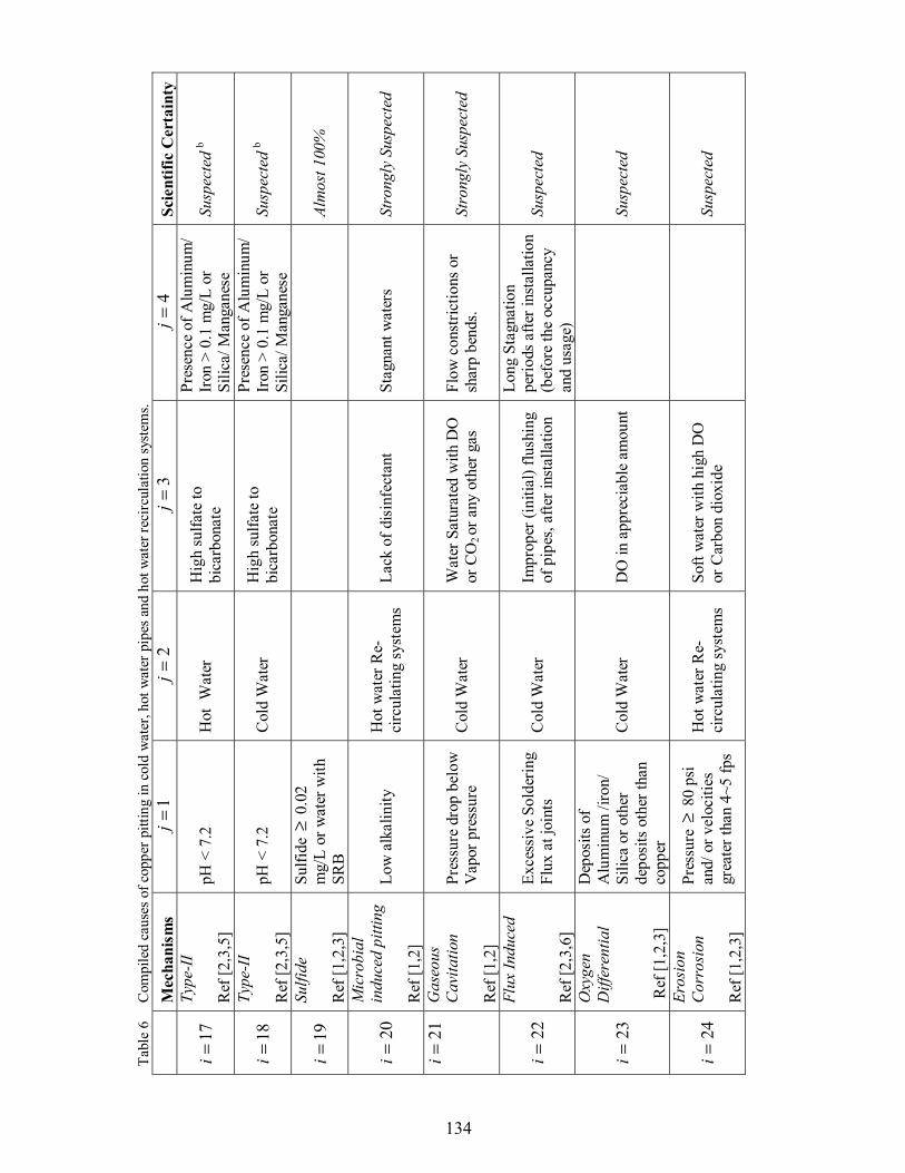
Tabl
e 6
C
ompi
led
caus
es o
f cop
per p
ittin
g in
col
d w
ater
, hot
wat
er p
ipes
and
hot
wat
er re
circ
ulat
ion
syst
ems.
M
echa
nism
s 1
=j
2=j
3
=j
4=j
Sc
ient
ific
Cer
tain
ty
17=i
Ty
pe-II
R
ef [2
,3,5
] pH
< 7
.2
Hot
Wat
er
Hig
h su
lfate
to
bica
rbon
ate
Pres
ence
of A
lum
inum
/ Ir
on >
0.1
mg/
L or
Si
lica/
Man
gane
se
Susp
ecte
d b
18=i
Ty
pe-II
R
ef [2
,3,5
] pH
< 7
.2
Col
d W
ater
H
igh
sulfa
te to
bi
carb
onat
e
Pres
ence
of A
lum
inum
/ Ir
on >
0.1
mg/
L or
Si
lica/
Man
gane
se
Susp
ecte
d b
19=i
Su
lfide
R
ef [1
,2,3
]
Sulfi
de ≥
0.0
2 m
g/L
or w
ater
with
SR
B
Alm
ost 1
00%
20=i
Mic
robi
al
indu
ced
pitti
ng
Ref
[1,2
]
Low
alk
alin
ity
Hot
wat
er R
e-ci
rcul
atin
g sy
stem
s La
ck o
f dis
infe
ctan
t St
agna
nt w
ater
s St
rong
ly S
uspe
cted
21=i
G
aseo
us
Cav
itatio
n R
ef [1
,2]
Pres
sure
dro
p be
low
V
apor
pre
ssur
e C
old
Wat
er
Wat
er S
atur
ated
with
DO
or
CO
2 or
any
oth
er g
as
Flow
con
stric
tions
or
shar
p be
nds.
Stro
ngly
Sus
pect
ed
22=i
Flux
Indu
ced
Ref
[2,3
,6]
Exce
ssiv
e So
lder
ing
Flux
at j
oint
s C
old
Wat
er
Impr
oper
(ini
tial)
flush
ing
of p
ipes
, afte
r ins
talla
tion
Long
Sta
gnat
ion
perio
ds a
fter i
nsta
llatio
n (b
efor
e th
e oc
cupa
ncy
and
usag
e)
Susp
ecte
d
23=i
Oxy
gen
Diff
eren
tial
Ref
[1,2
,3]
Dep
osits
of
Alu
min
um /i
ron/
Si
lica
or o
ther
de
posi
ts o
ther
than
co
pper
Col
d W
ater
D
O in
app
reci
able
am
ount
Susp
ecte
d
24=i
Eros
ion
Cor
rosi
on
Ref
[1,2
,3]
Pres
sure
≥ 8
0 ps
i an
d/ o
r vel
ociti
es
grea
ter t
han
4~5
fps
Hot
wat
er R
e-ci
rcul
atin
g sy
stem
s So
ft w
ater
with
hig
h D
O
or C
arbo
n di
oxid
e
Susp
ecte
d
134
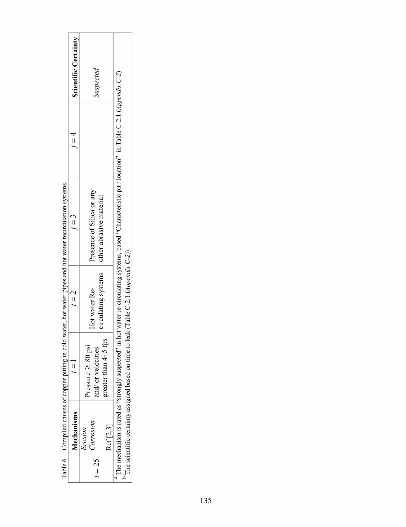
Tabl
e 6
C
ompi
led
caus
es o
f cop
per p
ittin
g in
col
d w
ater
, hot
wat
er p
ipes
and
hot
wat
er re
circ
ulat
ion
syst
ems.
M
echa
nism
s 1
=j
2=j
3
=j
4=j
Sc
ient
ific
Cer
tain
ty
25=i
Eros
ion
Cor
rosi
on
Ref
[2,3
]
Pres
sure
≥ 8
0 ps
i an
d/ o
r vel
ociti
es
grea
ter t
han
4~5
fps
Hot
wat
er R
e-ci
rcul
atin
g sy
stem
s Pr
esen
ce o
f Sili
ca o
r any
ot
her a
bras
ive
mat
eria
l
Susp
ecte
d
a Th
e m
echa
nism
is ra
ted
as “
stro
ngly
susp
ecte
d” in
hot
wat
er re
-circ
ulat
ing
syst
ems,
base
d “C
hara
cter
istic
pit
/ loc
atio
n” i
n Ta
ble
C-2
.1 (A
ppen
dix
C-2
) b
The
scie
ntifi
c ce
rtain
ty a
ssig
ned
base
d on
tim
e to
leak
(Tab
le C
-2.1
(App
endi
x C
-2))
135

136
Table 6 contains 25 mechanisms, these mechanisms and their attributes are
presented in form of a matrix ( i & j ) values. Each mechanism is identified with a
distinct i value that ranges from 1 through 25. The attributes for each mechanism are
identified with j values in the corresponding row; the j values range between 1 and 4.
The mechanisms presented in Table 6 are broadly grouped in three categories, namely,
with pH ≥ 7.8 ( =i 1 to 8), with pH < 7.8 ( =i 9 to 18) and mechanisms not dependant on
pH ( =i 19 to 25). The mechanisms ( =i 19 to 25) are either totally independent of pH or
their correlation with pH has not been reported. From Table 6, it can be inferred that for
each mechanism to occur, a set of constituents (corresponding =j 1 to 4) should co exist,
in a certain range. Since, the threshold values are not available in the literature, the
minimum value that is reported to have caused a failure is enlisted.
Hence, any jiX , or “attribute” (as used from now on) of the matrix in Table 6,
would define a particular parameter with a specified range / value, that forms a part of
recipe of the thi mechanism. Also all the pitting mechanisms require the co existence of
specific set of attributes. Hence, the “co existence” of a specific set of attributes becomes
a necessary condition for a particular mechanism.
Allocating scientific certainty to mechanisms
Although, the co-existence of a specific set of attributes becomes a necessary
condition for pitting to occur, but it is not essential that pitting would occur if this criteria
is met. This is established by the fact that there are other pipes that did not fail under the
same set of attributes. Hence, there exists a degree of uncertainty whether or not the

137
pitting will occur, even if all the required set of attribute coexists. This is expressed as
scientific certainty which is assigned on a linguistic scale in Table 6. The mechanisms in
Table 6, have been accumulated from more than one source where such a classification
may not have been made, hence following procedure was adopted to assign the scientific
certainties:
• The mechanisms identified in Table C-2.1 (Appendix C-2) (Dr Edwards personal
communication), already contain the scientific certainty assigned to each of them.
However, a separate mechanism ( 3=i in Table 6) is formulated for hot water
recirculation system with a scientific certainty “Strongly Suspected”, this was
based on the comments enlisted in “characteristic pit location” in Table C-2.1
(Appendix C-2). These comments elaborate that the mechanism is more severe in
hot water recirculation systems; hence a separate case with a stronger scientific
certainty is formulated.
• The mechanisms from Cohen and Myers, (1984) have been assigned the scientific
certainty based on the average time to leak (TTL) values. For all the mechanism
having a TTL less than 5 years are assigned “Strongly Suspected” category, for
mechanisms with TTL greater than 5 years and less than 20 years are assigned
“Suspected” category, all the mechanisms with TTL greater than 20 years are
assigned “Below Suspected” category.
• All the other mechanisms are assigned “Suspected” category.

138
An interpretation of these scientific certainties is explained as follows. The
maximum scientific certainty that can be assigned to any mechanism is “100%”, which
means that by following the recipe from Table 6, a pit can be artificially induced in the
laboratory. There is only one mechanism ( 1=i ) with a “100%” scientific certainty.
An “almost 100%” scientific certainty indicates that pitting with this recipe is
almost sure to occur, although none of the sources have reported to have verified the
recipe in a laboratory test to an extent of inducing a pinhole leak. Although, all the
sources have unanimously agreed that the recipe is extremely corrosive to copper. There
is only one mechanism ( 19=i ) with a “almost 100%” scientific certainty
The other scientific certainties include “Strongly Suspected”, “Suspected” and
“Below Suspected” categories, and these terms express likelihood of copper pitting on a
linguistic scale. These are mainly assigned based on time to leak, as explained previously.
The Scientific certainties of all the mechanisms are expressed in the last column of Table
6. These values or linguistic intensities will be utilized subsequently to obtain the scores
for each attribute.
To summarize, every row of matrix in Table 6 defines a particular pitting
mechanism, the attributes listed in the thi row ( =j 1 to 4) are the minimum number of
attributes that should co-exist as a necessary condition for the pitting to occur. Even if, all
the attributes of the thi row co-exist, the chances of pitting to occur will be the scientific
certainty expressed in last column of thi row.

139
Need of a numerical scale
The scientific certainties expressed in Table 6, are based on a linguistic scale of
verbal intensities. These certainties are linguistic hierarchies, which define the system
susceptibility in terms of the attributes. These intensities are not only subjected to ones’
interpretation but are also difficult to quantify in physical sense. It may be noted that the
terms used (such as “Suspected”) in a linguistic scale cover a range and are not mere
points on the intensity line (Figure 1). Although, the extents of the terms used in
linguistic scale (such as “Suspected” and “Strongly suspected”) may have well
demarcated boundaries in literal meaning but the boundaries for each term is not well
defined and quantifiable on an intensity line for the end user. This leaves zones of
overlap, where it becomes extremely difficult for the user to quantify the extent of the
problem in physical sense.
Figure 1 A schematic view of the linguistic scale, showing zones of verbal intensities.
Zones ofoverlap
Suspected Strongly Suspected
Nearly 100% 100%
Increasing Verbal Intensity
140
In real time situations, one or more attributes of a particular recipe may not be
present; the extent to which the system susceptibility to pitting would change becomes
totally unquantifiable in such situations. Thus, it becomes imperative to correlate these
pitting recipes and develop a scoring system for attributes that may be used with a
numerical scale and can provide quantifiable results to the user.
The advantage with the numerical scale is that the zones of overlap are
automatically eliminated. Although, to interpret results from a numerical scale, a
linguistic scale is almost necessary. Hence, an ideal situation will be a scoring system that
works on a numerical scale and that can yield quantifiable results which can ultimately be
correlated with the linguistic scale.
The following section presents a methodology of developing a scoring system for
attributes and a numerical scale, using the information from Table 6. The task to develop
a scoring system that incorporates the relative intensities of the attributes and which is
also consistent with the scientific certainties of each mechanism is divided into three
steps. First, a numerical scale is developed by defining ranges for scientific certainties on
a numerical scale with some unknown variables; these values are restricted by
formulating a set of mathematical constraints. Second, by using the relative intensities of
the attributes in Table 6, a set of mathematical constraints are formulated in terms of the
score ranges of the numerical scale, developed in first step. In the third step, the
mathematical constraints formed in the first and second step are solved simultaneously as
a goal program to achieve the scale parameters and the scores of the attributes.

141
Developing numerical scale
The purpose of developing a numerical scale is to provide a quantifiable basis for
scoring each attribute. As mentioned earlier, the numerical scale automatically eliminates
the zones of overlap between the two consecutive terms of linguistic scale. An example
of the numerical scale is shown in Figure 2.
Figure 2 A schematic view of the numerical scale, used in the present study.
Figure 2, is based on the assumption that the attributes shall assume only integral
scores. In order to avoid any overlap between the two consecutive terms on linguistic
scale a difference of unity is maintained. This line of demarcation (by unity) between the
two categories can only be maintained if all the attributes take integral values. If this
assumption is not made, the decimal values of the attributes would be obtained. As the
ultimate goal is to correlate the final scores of each mechanism with the linguistic scale,
the decimal values may not add any significant benefit. On the other hand, integral values
are easy to use; thus, the above assumption of integral values is adopted for developing
the numerical scale.
Increasing Score
b5 b3b7 b6
SuspectedStrongly Suspected 100%
b4
Below Suspected
b1
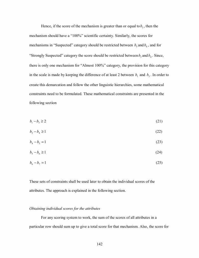
142
Hence, if the score of the mechanism is greater than or equal to 1b , then the
mechanism should have a “100%” scientific certainty. Similarly, the scores for
mechanisms in “Suspected” category should be restricted between 5b and 6b , and for
“Strongly Suspected” category the score should be restricted between 3b and 4b . Since,
there is only one mechanism for “Almost 100%” category, the provision for this category
in the scale is made by keeping the difference of at least 2 between 1b and 3b . In order to
create this demarcation and follow the other linguistic hierarchies, some mathematical
constraints need to be formulated. These mathematical constraints are presented in the
following section
231 ≥− bb (21)
143 ≥− bb (22)
154 =− bb (23)
165 ≥− bb (24)
176 =− bb (25)
These sets of constraints shall be used later to obtain the individual scores of the
attributes. The approach is explained in the following section.
Obtaining individual scores for the attributes
For any scoring system to work, the sum of the scores of all attributes in a
particular row should sum up to give a total score for that mechanism. Also, the score for

143
each mechanism should correspond to the value range of its scientific certainty on the
numerical scale. Hence, the total score obtained for any mechanism should be restricted
to a value range according to its scientific certainty. From Table 6, each attribute can be
identified by a set of ji & values. If the score corresponding to an attribute in thi row and
thj column is designated by jiX , , then the sum of the scores of the attribute in thi row
(designated by iS ) should be restricted to the value ranges in the numerical scale (Figure
2). This will lead to a system of inequalities that can be solved simultaneously to obtain
individual jiX , . These inequalities can be converted into equations using deviational
variables, and can be solved simultaneously using goal programming techniques.
The formulation of these inequalities using the score ranges of the numerical scale is
explained in Appendix D-2. Two formulations are shown below.
For 1=i (Cl2-Al-High pH)
The scientific certainty for the mechanism is “100 %”, hence the score 11 bS ≥ ,
14,13,12,11,1 bXXXX ≥+++ (26)
Using deviational variable, the inequality is converted into an equation. If 1d is a
deviational variable, then it can be expressed as the difference of two positive numbers,
hence
−+ −= 111 ddd (27)
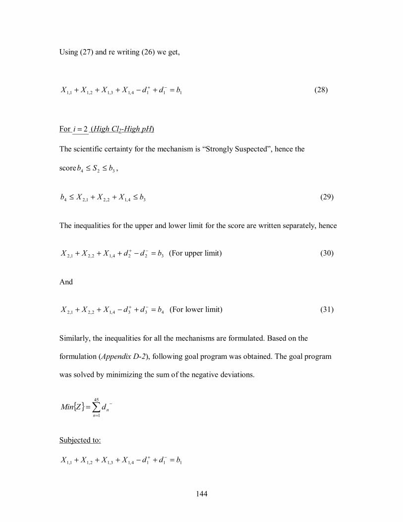
144
Using (27) and re writing (26) we get,
1114,13,12,11,1 bddXXXX =+−+++ −+ (28)
For 2=i (High Cl2-High pH)
The scientific certainty for the mechanism is “Strongly Suspected”, hence the
score 324 bSb ≤≤ ,
34,12,21,24 bXXXb ≤++≤ (29)
The inequalities for the upper and lower limit for the score are written separately, hence
3224,12,21,2 bddXXX =−+++ −+ (For upper limit) (30)
And
4334,12,21,2 bddXXX =+−++ −+ (For lower limit) (31)
Similarly, the inequalities for all the mechanisms are formulated. Based on the
formulation (Appendix D-2), following goal program was obtained. The goal program
was solved by minimizing the sum of the negative deviations.
∑=
−=45
1nndZMin
Subjected to:
1114,13,12,11,1 bddXXXX =+−+++ −+

145
4223,22,21,2 bddXXX =+−++ −+
3333,22,21,2 bddXXX =−+++ −+
4444,33,32,31,3 bddXXXX =+−+++ −+
3554,33,32,31,3 bddXXXX =−++++ −+
6664,43,42,41,4 bddXXXX =+−+++ −+
5774,43,42,41,4 bddXXXX =−++++ −+
6884,53,52,51,5 bddXXXX =+−+++ −+
5994,53,52,51,5 bddXXXX =−++++ −+
510103,62,61,6 bddXXX =−+++ −+
611113,62,61,6 bddXXX =+−++ −+
712124,73,72,71,7 bddXXXX =−++++ −+
713134,83,82,81,8 bddXXXX =−++++ −+
314144,93,92,91,9 bddXXXX =−++++ −+
415154,93,92,91,9 bddXXXX =+−+++ −+
616164,103,102,101,10 bddXXXX =+−+++ −+
517174,103,102,101,10 bddXXXX =−++++ −+
318184,113,112,111,11 bddXXXX =−++++ −+
419194,113,112,111,11 bddXXXX =+−+++ −+
521214,123,122,121,12 bddXXXX =−++++ −+
621214,123,122,121,12 bddXXXX =+−+++ −+
722224,133,132,131,13 bddXXXX =−++++ −+
323234,143,142,141,14 bddXXXX =−++++ −+
424244,143,142,141,14 bddXXXX =+−+++ −+
525254,153,152,151,15 bddXXXX =−++++ −+
626264,153,152,151,15 bddXXXX =+−+++ −+
727273,162,161,16 bddXXX =−+++ −+
528284,173,172,171,17 bddXXXX =−++++ −+
629294,173,172,171,17 bddXXXX =+−+++ −+
530304,183,182,181,18 bddXXXX =−++++ −+
631314,183,182,181,18 bddXXXX =+−+++ −+
1332321,19 +=+− −+ bddX 1133331,19 −=−+ −+ bddX
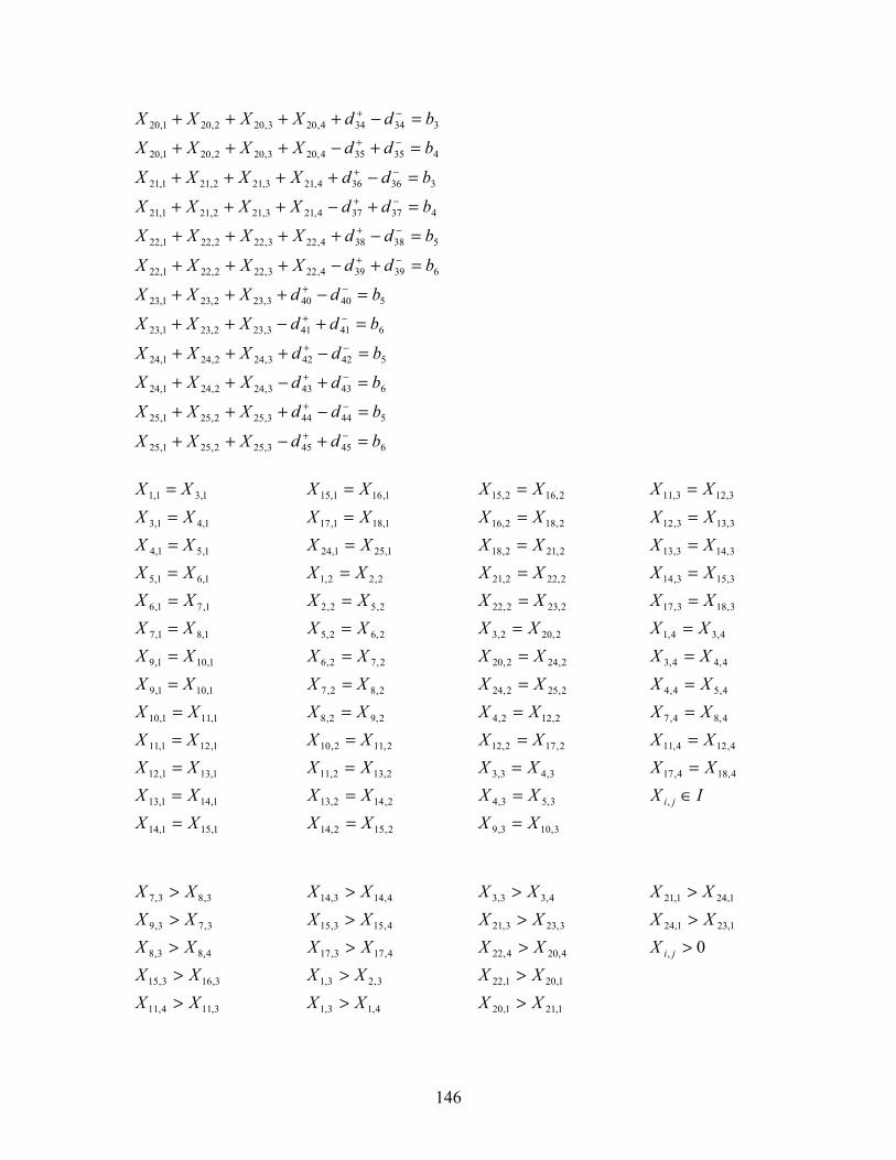
146
334344,203,202,201,20 bddXXXX =−++++ −+
435354,203,202,201,20 bddXXXX =+−+++ −+
336364,213,212,211,21 bddXXXX =−++++ −+
437374,213,212,211,21 bddXXXX =+−+++ −+
538384,223,222,221,22 bddXXXX =−++++ −+
639394,223,222,221,22 bddXXXX =+−+++ −+
540403,232,231,23 bddXXX =−+++ −+
641413,232,231,23 bddXXX =+−++ −+
542423,242,241,24 bddXXX =−+++ −+
643433,242,241,24 bddXXX =+−++ −+
544443,252,251,25 bddXXX =−+++ −+
645453,252,251,25 bddXXX =+−++ −+
1,31,1 XX = 1,41,3 XX = 1,51,4 XX = 1,61,5 XX = 1,71,6 XX = 1,81,7 XX = 1,101,9 XX = 1,101,9 XX = 1,111,10 XX = 1,121,11 XX = 1,131,12 XX = 1,141,13 XX = 1,151,14 XX =
1,161,15 XX = 1,181,17 XX = 1,251,24 XX =
2,22,1 XX = 2,52,2 XX = 2,62,5 XX = 2,72,6 XX = 2,82,7 XX = 2,92,8 XX =
2,112,10 XX = 2,132,11 XX = 2,142,13 XX = 2,152,14 XX =
2,162,15 XX = 2,182,16 XX = 2,212,18 XX = 2,222,21 XX = 2,232,22 XX =
2,202,3 XX = 2,242,20 XX = 2,252,24 XX =
2,122,4 XX = 2,172,12 XX =
3,43,3 XX = 3,53,4 XX = 3,103,9 XX =
3,123,11 XX = 3,133,12 XX = 3,143,13 XX = 3,153,14 XX = 3,183,17 XX =
4,34,1 XX = 4,44,3 XX = 4,54,4 XX = 4,84,7 XX =
4,124,11 XX = 4,184,17 XX =
IX ji ∈,
3,83,7 XX > 3,73,9 XX > 4,83,8 XX >
3,163,15 XX > 3,114,11 XX >
4,143,14 XX > 4,153,15 XX > 4,173,17 XX >
3,23,1 XX > 4,13,1 XX >
4,33,3 XX > 3,233,21 XX > 4,204,22 XX >
1,201,22 XX > 1,211,20 XX >
1,241,21 XX > 1,231,24 XX >
0, >jiX

147
231 ≥− bb 143 ≥− bb
154 =− bb 165 ≥− bb
176 =− bb Ibi ∈
3,24,13,1 XXX >+ 4,33,33,2 XXX +> 3,64,33,3 XXX >+ 4,73,73,6 XXX +>
4,83,84,73,7 XXXX +>+ 4,93,94,113,11 XXXX +>+
4,143,144,93,9 XXXX +>+ 4,103,104,143,14 XXXX +>+ 4,153,154,103,10 XXXX +>+ 4,173,174,153,15 XXXX +>+ 4,133,134,173,17 XXXX +>+
3,164,133,13 XXX >+
The above goal program is solved using software “LP solve”, the program is available for
download on http://www.statslab.cam.ac.uk/~rrw1/opt/lp_solve/.
Results and Discussions
The summary of results is presented in Table 7 and Table 8. The values of the deviational
variables are,
Deviational variables
0=−id , For all ]45,1[∈i
37816212527283138404244 ============ ++++++++++++ dddddddddddd ,
22419233436 ====== ++++++ dddddd ,
113142215 ==== ++++ dddd
0242629303233353739414345 ============ ++++++++++++ dddddddddddd
0135610111239171820 =========== +++++++++++ ddddddddddd

148
Scale parameters
241 =b , 223 =b , 204 =b , 195 =b , 166 =b , 157 =b
Table 7 Score ranges for scientific certainties.
Scoring Criteria Scientific Certainty
15≤Sum Below Suspected 1916 ≤≤ Sum Suspected
2220 ≤≤ Sum Strongly Suspected 23=Sum Almost 100% 24≥Sum 100%
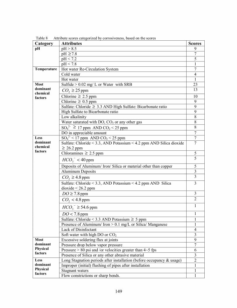
149
Table 8 Attribute scores categorized by corrosiveness, based on the scores Category Attributes Scores
pH > 8.5 9 pH ≥ 7.8 7 pH < 7.2 5
pH
pH < 7.8 1 Hot water Re-Circulation System 7 Cold water 4
Temperature
Hot water 1 Sulfide > 0.02 mg/ L or Water with SRB 23
252 ≥CO ppm 13 Chlorine ≥ 2.5 ppm 10 Chlorine ≥ 0.5 ppm 9 Sulfate: Chloride ≥ 3.3 AND High Sulfate: Bicarbonate ratio 9 High Sulfate to Bicarbonate ratio 9 Low alkalinity 8 Water saturated with DO, CO2 or any other gas 8 SO4
2- ≥ 17 ppm AND CO2 < 25 ppm 8
Most dominant chemical factors
DO in appreciable amount 7 SO4
2- < 17 ppm AND CO2 < 25 ppm 7 Sulfate: Chloride < 3.3, AND Potassium < 4.2 ppm AND Silica dioxide ≥ 26.2 ppm
7
Chloramines ≥ 2.5 ppm 5 403 <−HCO ppm 5
Deposits of Aluminum/ Iron/ Silica or material other than copper 5 Aluminum Deposits 3
8.42 ≥CO ppm 3 Sulfate: Chloride < 3.3, AND Potassium < 4.2 ppm AND Silica dioxide < 26.2 ppm
3
8.7≥DO ppm 3 8.42 <CO ppm 2
6.543 ≥−HCO ppm 1
8.7<DO ppm 1 Sulfate: Chloride < 3.3 AND Potassium ≥ 5 ppm 1 Presence of Aluminum/ Iron > 0.1 mg/L or Silica/ Manganese 1 Lack of Disinfectant 4
Less dominant chemical factors
Soft water with high DO or CO2 3 Excessive soldering flux at joints 9 Pressure drop below vapor pressure 7 Pressure > 80 psi and /or velocities greater than 4~5 fps 6
Most dominant Physical factors Presence of Silica or any other abrasive material 3
Long Stagnation periods after installation (before occupancy & usage) 2 Improper (initial) flushing of pipes after installation 1 Stagnant waters 1
Less dominant Physical factors Flow constrictions or sharp bends. 1

150
Based on the scores, each attribute is classified into most dominating or less
dominating category. Thus the scoring system helps in broader classification of the
chemical and physical parameters. Although, certain lesser dominant factors can produce
adverse affects in combination with pH, temperature or other attributes from most
dominant category.
The interpretation of the scores should be done based on Table 6, 7 and 8. The
present scoring system works on the minimum number of attributes. This is because each
mechanism in Table 6 is defined based on minimum number of attributes that are
required to produce a pinhole leak failure. Hence, the scores in Table 8 should be
combined only for specific mechanisms that are defined in Table 6.
Formulations based on maximum number of attributes were attempted, but since
some of the attribute change behavior with pH and temperature, such scoring system
could not be formed. The inconsistency in the attempted formulation was mainly due to
the behavior of sulfate and chlorine. Since, sulfate is dominant in pH < 7.8 range, and it
does not contribute in pitting at pH 8.7≥ range. This is primarily because increased
solubility of brochantite scale at high pH values.
Similarly, chlorine is corrosive at high pH values (> 7.8) especially if aluminum
deposits are present the synergy between aluminum and chlorine produces most corrosive
combination. However at low pH (< 7.8) range none of the sources in the literature have
reported any failure due to chlorine and aluminum. Most importantly, the role of sulfate
151
is highly dependant on relative concentration between sulfate and chloride, the three
zones of synergy were explained previously in the chapter. Hence, for a sulfate
concentration of about 17 ppm, and sulfate the chloride ratio of about 3.3, the chloride
concentration work out to be 5.65 ppm, which needs to be constrained as not corrosive
under low pH concentration during the formulation. Due to this anomaly, the scoring
system in the above problem is constrained and hence the use of Table 6 becomes
necessary with Table 7 and Table 8.
Conclusions
The study concludes in identifying the chemical and physical parameters that are
mainly responsible for causing copper failures in home plumbing. The role of water
chemistry seems dominant in copper pitting but there are other hydraulic and physical
parameters that can act in synergy to produce adverse effects. The exact causal
mechanism of the copper pitting is not clear; this is due to lack of a unified theory. In the
absence of such a mechanistic theory, the parameters that are responsible for copper
pitting may be classified into dominant and lesser dominant categories based on the
scoring system.
Due to variability in water chemistry the system susceptibility should be gauged
based on the water quality at the tap. The scoring system can be used to gauge the system
susceptibility. The system susceptibility should be gauged based on the mechanism that
provides the maximum score for a particular plumbing system. For the homes where the
pinhole leak has not occurred in past, the scoring system should be used only for advisory

152
purposes. However, for the homes that have a previous history of pinhole leaks, the
scoring system can provide good quantifiable results. The scoring system can identify the
most critical mechanism for a particular plumbing system, and hence can be used to
device suitable preventive action against future pinhole leaks. The combination of the
scores should be done based on Table 6; other combinations should not be used for
evaluation.
References
1. Personal communication with Dr Marc Edwards (Professor Civil and
Environmental Engineering Department, Virginia Tech, Blacksburg- VA 24061)
2. Copper Development Association (CDA), Failure reports 1975~2004.
3. Myers J and Cohen A (2005) Copper-tube Corrosion in Domestic Water Systems.
Boiler systems engineering (American Boiler Manufacturer’s Association).
4. Cohen A. and J R Myers, (1984) Mitigation of Copper tube Cold water pitting by
Water Treatment, Corrosion, NACE International, Houston, TX.
5. Edwards M., Ferguson J.F., Reiber S.H.(1994) The Pitting Corrosion of Copper.
Journal of AWWA 74-90
6. Rossum J.R (1985), Pitting in Copper Water Tubing, Journal of the AWWA,
October, 1985, 70-73.
7. Handbook on copper by ASM International (2001), 154-155, 385-415.
8. Internal corrosion of water distribution system, AWWA 1996, 1-27, 231-268.

153
9. Handbook of Corrosion Engineering, Roberge P.R., 2000, 331-369.
10. Edwards M. and Jacobs S. (2000) Sulfide Scale Catalysis of Copper Corrosion.
Water Resources Research 34, 2798-2808.
11. Edwards M, and Rushing J C (2004) Effect of aluminum solids and chlorine on
cold water pitting of copper. Corrosion Science 46, 3069-3088.
12. Duthil J.P., Giusti A. and Mankowski G.(1997) The pit Morphology on Copper in
Chloride and Sulfate Containing Solutions. Corrosion Science 39, 27-42.
13. Duthil J.P., Giusti A. and Mankowski G.(1996) The Synergetic Effect of Chloride
and Sulfate on Pitting Corrosion of Copper. Corrosion Science 38, 1839-1849.
14. Sobue K., Sugahara A., Nakata T., Imai H., Magaino S.(2003) Effect of Carbon
Dioxide on Corrosion Behavior of Copper in Simulated Water. Surface and
Coatings Technology 169-170, 662-665.
15. Warakky A. El, Shayeb H.A.El, Sherif E.M.(2004) Pitting Corrosion of Copper in
Chloride Solutions. Anti Corrosion Methods and Materials 51 (1), 52-61.
16. Ellis II Peter F. (2000) Pitting Corrosion in Domestic Copper Plumbing- The Rise
and Fall of the “Pitting Water” Theory. NACE Corrosion (# 00652)
17. Edwards M., Rehring J., Meyer T. (1994), Inorganic Anions and Copper Pitting.
NACE Corrosion, 50 (5), 366-372.
18. Schock M.R. (1999), Internal Corrosion and Deposition Control. Water Quality
and Treatment- AWWA (1999), Chapter 17.
154
19. Cohn P.D., Cox M., Berger B. S. (1999), Health and Aesthetic Aspects of Water
Quality. Water Quality and Treatment- AWWA (1999), Chapter 2.
20. Letterman R.D., Amirtharajah A., O’Melia C.R.(1999), Coagulation and
Flocculation. Water Quality and Treatment- AWWA (1999), Chapter 6.
21. Haas C.N. (1999), Disinfection. Water Quality and Treatment- AWWA (1999),
Chapter 14.
22. Sulfur Bacteria, Manual for Water Supply Practices M 7. AWWA (2003) 17-22.
23. Cohen A., Lyman S, (1972), Service Experience with Copper Plumbing Tube.
Materials Protection and Performance 11 (2), 48-53.
24. Edwards M., Rushing J.C., Kvech S., Reiber S., Assessing copper pinhole leaks in
residential plumbing. Water Science and Technology 49 (2), 83-90.
25. Peavy H.S., Rowe D.R., Tchobanoglous G. (1985). Environmental Engineering-
McGraw Hill Book Co. 1-45, 109-204.
26. Tchobanoglous G., Schroeder E.D., (1985). Water Quality-Addison Wesley
Publishing Co. 43- 179.
27. Viessman, W. Jr., Hammer M. J (1993). Water Supply and Pollution Control-
HarperCollins College Pub. 396-455
28. Zhe Y., Pehkonen S.O., (2004). Copper Corrosion Kinetics and Mechanisms in
the presence of Chlorine and Orthophosphate. Water Science and Technology- 49
(2). 73-81.
29. Maryland Task Force Study, Final Report (2004).

155
30. Nguyen, C.K. 2005. Interactions Between Copper and Chlorine Disinfectants:
Chlorine Decay, Chloramine Decay and Copper Pitting. Masters’ Thesis,
Virginia Tech.
31. American Water Works Association (AWWA) and American Water Works
Association Research Foundation (AWWARF), Utility Survey- Water Stats
(1996).
Website References
32. http://www.epa.gov
33. http://www.awwa.org
34. http://www.statslab.cam.ac.uk
35. http://corrosion.ksc.nasa.gov

Appendix A-2
156
APPENDIX A-2
Types of corrosion of copper

Appendix A-2
157
Types of corrosion
The handbook on copper metal published by ASM International (2001) contains
comprehensive details about metallurgical properties of copper and its uses in various
applications. It identifies nine types of corrosive attacks that can cause corrosion in
copper. An overview of these types of corrosive attacks is presented.
General corrosion
This type of attack occurs over the entire surface at almost a uniform rate, hence it
is often known as uniform corrosion. It results due to prolonged contact of the metal
surface with its environment. The associated rate of corrosion is generally low and hence,
this type of corrosion is considered least damaging to copper. In drinking water pipes,
this type of corrosion seldom causes any failure, however, if severe, it may lead to high
levels of leaching of copper, typically causing “Blue-water” or “Green-water” problems.
Uniform corrosion rapidly increases with decrease in pH, it is significant in acidic waters
(pH< 6), and may cause high soluble copper concentrations (> 1.3 mg/L) without the
evidence of “green or blue” water (AWWA 1996). At higher pH (> 7), the rate of the
uniform corrosion is very small, mostly at pH exceeding 7, the copper corrosion is
considered to be non uniform (AWWA 1996). Soft waters in pH range 6 to 7 may cause
uniform corrosion, often the phenomenon is associated to the high concentration of
carbon dioxide in the said pH range, however, there is “considerable disagreement” on
the role of carbon dioxide in copper corrosion (AWWA 1996). The present work is
related to the non uniform corrosion of copper; hence uniform corrosion will not be
discussed henceforth.

Appendix A-2
158
Galvanic Corrosion
This type of corrosion occurs when two dissimilar metals are connected and
immersed in a conductive solution. This is due to the formation of an electrochemical cell
because of the differences in electrode potential. The metal that is nobler becomes the
cathode and the less noble metal becomes the anode and gets consumed in the
electrochemical reaction. The surface area ratio of the anode and the cathode is important
(Roberge 2000), if the surface area ratio of anode to cathode is small, he corrosion
current may be concentrated over a small anodic area, hence may cause dissolution from
that small area. The galvanic series of the metals from National Aeronautics and Space
Administration (NASA) is available on http://corrosion.ksc.nasa.gov/galcorr.htm . The
series id presented in Table A-2.1.
Copper in general is noble (cathodic) to most of the other metals used in the water
distribution system and hence less likely to corrode. However, in certain specific
conditions the metals like stainless steel exhibit variable behavior, that is, it may be
anodic or cathodic to copper, depending upon the conditions of its exposure (ASM
Handbook 2001). Hence, under these circumstances copper may become anodic to
stainless steel and thus undergo corrosion. In general, galvanic corrosion is not very
common in copper pipes that are used in home plumbing; however, it is generally
recommended that the contact between the copper pipe and the other metal should be
avoided.

Appendix A-2
159
Table A-2.1 Galvanic series of metals and alloys (source NASA) Platinum Gold Graphite Silver 18-8-3 Stainless steel, type 316 (passive) 18-8 Stainless steel, type 304 (passive) Titanium 13 percent chromium stainless steel, type 410 (passive) 7NI-33Cu alloy 75NI-16Cr-7Fe alloy (passive) Nickel (passive) Silver solder M-Bronze G-Bronze 70-30 cupro-nickel Silicon bronze Copper Red brass Aluminum bronze Admiralty brass Yellow brass 76NI-16Cr-7Fe alloy (active) Nickel (active) Naval brass Manganese bronze Muntz metal Tin Lead 18-8-3 Stainless steel, type 316 (active) 18-8 Stainless steel, type 304 (active) 13 percent chromium stainless steel, type 410 (active) Cast iron Mild steel Aluminum 2024 Cadmium Alclad Aluminum 6053 Galvanized steel Zinc Magnesium alloys Magnesium
Corroded end (anodic or least noble)
Non-corroded end (cathodic, or most noble)

Appendix A-2
160
Pitting Corrosion
Like other metals, copper undergoes pitting when exposed to certain conditions.
The pitting corrosion may be localized or may be spread over the entire area. When
spread over a large area, it roughens the surface and makes it irregular; in addition it may
cause significant weight loss of the metal from the surface. However, localized pitting is
considered to be the most dangerous form of corrosion, it is generally confined to a
smaller area with pits of various shape and sizes. The weight loss due to localized pitting
may not be significant but it may cause failures in a shorter time frame. Copper metal is
susceptible to pitting mainly due to surface non-uniformity (metallurgical reasons) and
due to environmental factors.
The pitting corrosion of copper is not completely understood with respect to
environmental conditions. Even today, the pitting is considered somewhat random in
terms of its occurrence and location. Copper pitting is a major concern in home plumbing
systems. It has been reported in United States, Canada, Germany and other European
countries. Despite of significant research, copper pitting is not completely understood. A
detailed overview of the causes of the pitting that are reported in the literature is
presented later in the section.
Crevice Corrosion is another form of localized corrosion which occurs near the
crevice formed by two metals (copper and any other) or between the crevice formed by
copper and any non metal. The attack is similar to pitting attack in terms of its
unpredictable nature with respect to the location of its occurrence. Crevice corrosion may

Appendix A-2
161
also result due to accumulation of foreign objects (dirt, vegetation or debris) on the
surface of the metal. In home plumbing systems, it is often termed or water line attack or
oxygen differential cell corrosion. In copper water lines, the attack generally occurs
below the silica, aluminum or deposits of foreign material (other than copper) due to the
differential in the oxygen concentration. The layer below the debris or the deposits is
oxygen deficient with respect to the surface of the debris on the water side. This results in
different electrochemical potential on two sides of the debris (AWWA 1996), the
corrosion occurs to equalize the two potentials. The part of metal with high oxygen
concentration acts as cathode, while the metal in contact with lower oxygen concentration
becomes the anode (AWWA 1996). Since, the oxygen is not produced at either anode of
cathode, the corrosion proceeds in such a way that the higher oxygen concentration is
reduced (Uhlig 1938), if the pH is same on both the sides. Due to the resistance in
diffusion of oxygen because of the debris or distance of transport, the differential in
oxygen between the two layers is maintained; this continues the corrosion attack at low
oxygen sites, leading to deepening of crevice in form of pitting (AWWA 1996).
Impingement
This type of attack occurs when the liquid, vapors or gases impinge the copper
surface with high velocities. This attack is related to the flow conditions (velocity,
pressure and temperature) of water. It is also dependant on the flow geometry
(constrictions in flow, sharp bends in flows etc). It may be sub classified into Gaseous
Cavitation and Erosion Corrosion. Gaseous Cavitation occurs due to impingement of
bubbles (gases) on the inner pipe wall. Water may be assumed to be a two phase liquid,

Appendix A-2
162
the gases (chlorine, oxygen etc) are dissolved in water and remain in equilibrium based
on Henry’s Law. The equilibrium concentrations of these dissolved gases are dependant
on the pressure and temperature of the water. Due to increase in flow velocities (or drop
in pressure) these gases may leave the liquid phase which results in degasification of
water. The gases escape in form of bubbles that subsequently collapse after hitting the
pipe walls. The pressure developed under the conditions of bubble collapse is extremely
high and destroys the protective film of copper. The phenomenon is more prominent near
sharp bends and flow constrictions. At higher temperatures, the capacity of the water to
retain these gases decreases substantially.
Erosion Corrosion occurs when the flow velocities are higher than 4~5 fps,
typically these conditions can occur under high street level pressures (greater than 80
psi), sharp irregularities at joints (due to poor workmanship or unreamed edges) or at
flow constrictions, where the liquid jet constantly hits the pipe wall and damages the
protective layer of copper. The phenomenon may be aggravated due to presence of
dissolved oxygen and carbon dioxide due to the removal of protecting film and formation
of concentration cells that subsequently form anodic sites, locally. Impingement is a
common cause of copper tube failures in hot water recirculation systems; however
incidences in cold water pipes are also reported in the literature.
Fretting
This form of attack appears in the form of pits or grooves marked by presence of
corrosion products. This attack is associated with the surfaces that are subjected to
Appendix A-2
163
repetitive (sliding) motion with other surface and the interface is subjected to some
external load in presence of oxygen and moisture. All the three conditions, that is,
relative motion between surfaces, external load, moisture and oxygen are necessary
conditions for fretting corrosion to occur. Fretting is not a common type of corrosion in
copper and copper alloys. In copper home plumbing systems, it is not of significance due
to the absence of at least one of the necessary conditions.
Inter-granular Corrosion
This type of corrosion is associated with the metals that are subjected to exposure
to high pressure steam. The corrosion occurs such that it penetrates the metal surface
often to the depth of metal grains. This attack is associated with the chemical segregation
effects (impurities present in the metal surface) (Roberge 2000). The form of corrosion is
not relevant to home plumbing systems, hence it will be kept out of the scope of the
present study.
De-alloying Corrosion
It is the process of removal of more active metal selectively from an alloy. This
leaves behind a weak deposit of the more noble metal. It is generally observed in alloys
like brass (dezincification of brass), aluminum and nickel. In general, the attack is more
common in alloys having a significant proportion of more active (cathodic) metal. Since,
the copper tubes used in home plumbing have more than 99.9% copper, these tubes are
not susceptible to de-alloying attack.
Appendix A-2
164
Corrosion Fatigue
The combined action of corrosion (usually pitting) and cyclic stress may cause
corrosion fatigue. This results in cracking of the metal, usually at right angles to the
applied tensile stress. This type of failure usually involves more than one parallel cracks
resulting into a failure of the metal. These cracks generally, originate from corrosion pits
and may be finer and invisible to naked eye. These cracks are distinctly different from the
cracks originated solely due to stress or cyclic stress cracks, as the latter generally does
not involve more than one crack. Copper and copper alloys are fairly resistant to
corrosion fatigue, and hence this type of failure is not considered in detail in the present
study.
Stress-Corrosion Cracking
This type of corrosion occurs when the metal is subjected to combined effects of
sustained stress and certain chemical substances. These chemical substances include
ammonia, in presence of oxygen or carbon dioxide and moisture. These conditions are
often met by underground copper service lines that corrode due to presence of the said
chemicals and moisture in the soil. Since, the nature of these failures related to home
plumbing is limited to failures that initiate from the outer side of the pipes; these failures
are not considered in detail in the present work.
Another class of corrosion that is not defined in ASM handbook is microbiologically
induced corrosion. An overview of microbiologically induced carrion is presented.

Appendix A-2
165
Microbiologically induced corrosion
This is a general class of corrosion, due to the result of bacterial and microbial
interaction of the pipe wall. Microbiological induced corrosion (MIC) may cause
degradation of pipe wall and problems like taste and odor issues. The growth (algae or
fungi) may cause corrosion by influencing several parameters like pH, dissolved oxygen
(Schock, 1999). The areas in the vicinity of pipe wall may contain different families of
bacteria or microorganism species that are often shielded by the deposits or tubercules of
corrosion products and find protection against the disinfectants or dissolved oxygen. The
stagnant waters, dead ends in pipes and lower level of disinfectant residuals sometimes
provide ideal breading ground for these species. The nature of the attack due to these
bacteria and microbial activities sometimes necessitates mechanical cleaning before
substantial control can be achieved through residual disinfectant (Schock, 1999). There
are number of ways in which the bacteria can cause corrosion. The nitrifying bacteria can
consume dissolved oxygen, cause oxygen concentration cells that produce lower pH and
eventually causing localized or pitting corrosion (Schock, 1999).
Appendix B-2
166
APPENDIX B-2
Chemical parameters affecting copper pitting (Contd. from Chapter-2)

Appendix B-2
167
Chemical parameters affecting copper pitting
The following discussion is a continuation of the chemical parameters discussed in
Chapter-2.
Nitrate
Nitrate ion [NO3-] is generally not aggressive to copper (Edwards et al. 1994).
Importantly, nitrate is a contaminant and is regulated by USEPA national primary
drinking water standards. The maximum contaminant level (MCL) for nitrate set by
USEPA is 10 mg/ L. The consumption of nitrate above the MCL can pose serious health
hazards to infants below the age of six months, the illness may be fatal if not treated
(USEPA).The symptoms include shortness of breath and blue-baby syndrome.
From copper corrosion perspective, low levels of nitrates decrease the pitting
frequency, while higher levels (> 40 mg/ L) of nitrate may increase the pitting frequency
(Edwards et. al 1994). Since, such higher levels (> 40 mg/ L) are well beyond the
maximum contaminant limit (< 10 mg/ L), these concentrations are not expected in
finished drinking water. Pitting failures due to nitrates are rarely known, the CDA reports
have never identified nitrates as the cause of the failure.
The AWWARF/ AWWA utility survey provides a range for nitrate concentration
for finished ground and surface waters. The nitrate concentration for finished grond water
varies 0 and 81 mg/L. The nitrate concentration for finished surface water varies between
0 and 25 mg/L. The range exceeds the maximum contaminant limit of 10 mg/L, enforced

Appendix B-2
168
by USEPA primary standards. The cause of such higher concentrations of nitrates is not
explained in the data.
Hydrogen Sulfide
Hydrogen sulfide is one of the most severe corrosive agents for copper. Sulfide is
a natural constituent in well waters, resulting from the bacterial decomposition of sulfur
in soil or in bed rocks. The process of reduction is facilitated by a class of bacteria known
as sulfate reducing bacteria (SRB). The sulfate reducing bacteria grow by using large
quantities of sulfur, sulfates and / or other forms of oxidized sulfur to generate hydrogen
sulfide gas (AWWA, 2003). The presence of hydrogen sulfide or SRB in waters is often
marked by bad odor “rotten eggs”; however, this smell is not typical as this smell is often
associated with other bacteria, including many coliforms (AWWA, 2003). These bacteria,
generally grow in anaerobic conditions, and vent hydrogen sulfide in water in the absence
of dissolved oxygen (AWWA, 2003). A possible remedy to remove hydrogen sulfide and
/ or SRB is to increase dissolved oxygen (AWWA, 2003).
It can thus be inferred that the presence of hydrogen sulfide and/ or sulfate
reducing bacteria can be very lethal from pitting perspective. This could lead to sulfide
attack that could suddenly become severe (Schock, 1999). Copper failures in some parts
of Florida are mainly due to the presence of sulfide in ground water. As the water in these
utilities is withdrawn from deep aquifers, it is understandable that it provides ideal
anaerobic conditions for SRB to flourish.
Appendix B-2
169
The attack by hydrogen sulfide is complex, very often the attack is not apparent
for months and then it suddenly becomes severe (Schock, 1999). Interestingly, all the
sources in the literature as well as the CDA reports have unanimously identified sulfide
as the species that can cause copper failures almost single handedly. The sulfide attack is
generally multi pronged, the presence of sulfide catalyzes the rate of corrosion in copper
by about 1 ~2 orders at wide pH ranges (6.5 and 9.2) (Jacobs and Edwards, 2000),
additionally, it prevents the formation of protective scale on copper surface. In presence
of sulfide, the scale formed is thick, black and poorly adheres to copper surface (Jacobs
and Edwards, 2000). The scale may contain cuprous sulfide [Cu2S] or cupric sulfide
[CuS] or other non stoichiometric species of copper sulfide (McNeil et al. (1993) and
(1991)).
It is due to these factors that sulfide poses the greatest threat to copper as
compared to other water quality parameters like chlorine, alkalinity, pH (Jacobs and
Edwards, 2000). The threshold concentrations that can cause copper failure are not
known but concentrations as low as 0.02 mg/ L are found to induce a leak in copper tubes
(Myers and Cohen, 2005). The copper sulfide attack is often accompanied by “black
water” problems; it is mainly due to the loosely attached sulfide scale on the copper
surface.
The AWWARF/ AWWA utility survey does not provide any data for sulfide in finished
ground or surface waters.

Appendix B-2
170
Chloride, Chlorine and Chloramines
Chlorine is a strong oxidizing agent; it is widely used for disinfection in utilities
irrespective of the source of water. During the disinfection process, chlorine is either
added in gaseous form or it is added as solids i.e. sodium or calcium hypochlorite (Peavy,
1985).The following equations described the formation of hypochlorous acid and
hypochlorite ion,
−+ ++⇔+ ClHHOClOHCl 22 (B1)
+− +⇔ HOClHOCl (B2)
If chlorination involves addition of solid sodium or calcium hypochlorite, then the
equations are,
−+ +→ OClNaNaOCl (B3)
( ) −+ +→ OClCaOClCa 222 (B4)
OHCleHOCl 222 +→++ −−+− (B5)
The relative amount of chlorine present in chlorine gas or hypochlorite (of
calcium or sodium) is expressed in terms of available chlorine (Haas, 1999). The
concentration of hypochlorite may be determined by calculating electrochemical
equivalent amount of Cl2 to that compound. For example,
−− ⇔+ CleCl 222 (B6)

Appendix B-2
171
From Eqn (B6), one mole of elemental chlorine reacts with two electrons to form
chloride, Eqn (B5) shows that one mole of hypochlorite will react with two electrons to
form chloride ion, hence, one mole of hypochlorite is electrochemically equivalent to one
mole of elemental chlorine and it can be said to have 70.91 g of available chlorine (Haas,
1999). Hence, calcium hypochlorite contains two moles of elemental chlorine, i.e. 141.8
g of available chlorine. If the available chlorine is divided by the molecular weights of
calcium hypochlorite (143 g/ mol) and sodium hypochlorite (74.5 g/ mol), it shall yield
the percentage of free chlorine in the compound. Hence, available chlorine for calcium
hypochlorite is 99.2 percent and for sodium hypochlorite available chlorine is 95.8
percent by weight.
The dissociation of hypochlorous acid (Eqn B2) is primarily dependent on pH and
temperature. The formation of hypochlorous brings down the pH of the solution, which
restricts the formation of hypochlorite ion after one point (Peavy, 1985). When chlorine
is added in solid form, the dissociation of hypochlorite ion (Eqn B5) causes rise in pH
(Peavy, 1985). However, the change in pH in both these conditions is highly dependant
on the buffer intensity and pH of the water. If water has sufficient dissolved inorganic
carbon (DIC), it is like to provide a buffer against change in pH, with exceptions to pH
near 8, where the buffer intensity is the minimum.
The sum of the hypochlorous acid and the hypochlorite ion is called free chlorine
residual. And the sum of molecular chlorine (Cl2), hypochlorous acid and hypochlorite

Appendix B-2
172
ion is generally called free available chlorine. The combined available chlorine residual
is the residual existing in chemical combination with ammonia or organic nitrogen
compounds (Viessman, 1993).
USEPA regulates the maximum disinfectant residual levels to 4.0 mg/ L
(measured as Cl2), the item is in the national primary standards and hence legally
enforceable. Increase chlorine residuals in water may pose health hazards that include
eye/ nose irritation and stomach discomfort (USEPA). Chlorine gas is highly toxic to
humans, since it is heavier than air it spreads slowly at ground level. Due to this reason,
sometimes use of hypochlorites is mandated, especially if the treatment plant is located
nearly populated areas (Peavy, 1985). Chlorine is a strong oxidizing agent, during the
process of disinfection sometimes it reacts with natural organic matter to produce certain
products that are not desirable and are carcinogenic to humans. These products are called
disinfection byproducts (DBP). The main DBPs are Trihalomethanes (measured as total
trihalomethane) TTHM and Haloacetic acid five (HAA5). USEPA, enforced the
disinfection byproduct rules (stage-I) in the year 1998, the rule required the reduction of
specific percentage of organic matter from finished water, in addition the rule enforced
new limits on total trihalomethans and haloacetic acid.
Due to the enforcement of the D/ DBP rule, many utilities changed the
disinfectant from chlorine to chloramines. Chloramines are the product of hypochlorous
acids and ammonia. Chloramines primarily consist of three forms, monochloramine

Appendix B-2
173
[NH2Cl], dichloramine [NHCl2] and nitrogen tetrachloride or trichloramine [NCl3]. The
equations leading to formation of chloramines are,
OHClNHHOClNH 223 +→+ (B7)
OHNHClHOClClNH 222 +→+ (B8)
OHNClHOClNHCl 232 +→+ (B9)
The chloramines residual is an identified contaminant in drinking water and is
regulated in national primary standard. In most of the drinking water, the primary
chloramines species is monochloramine (Cohn, 1999). The adverse health effects due to
the consumption of chloramines have been limited to hemodialysis patient (Cohn, 1999).
In the background of the disinfection process, the role of chloride, chlorine and
chloramines is examined with respect to copper pitting. The formation of chloride [Cl-] is
the direct result of addition of either gaseous or solid chlorine in water. Other than the
disinfection process, the possible source of chloride could be dissolved inorganic ionic
compounds of [Cl-] anion. These solids may ionize in aqueous solution providing
chloride ions. USEPA has enlisted chloride in the national secondary standards. Chloride
concentration exceeding 250 mg/ L is likely to cause salty taste in drinking water.
Researchers have repeatedly identified chloride as the major culprit leading to copper
pitting; this hypothesis is overwhelmingly supported by the CDA reports where chloride
induced pitting emerged as the largest cause of failure in cold water pipes. The sources of
chloride identified by CDA are primarily the soldering flux and/ or the strong oxidizing
agents used in disinfection, namely, gaseous chlorine, sodium hypochlorite, calcium

Appendix B-2
174
hypochlorite and chlorinated cyanurates. The CDA reports identify chloride as the cause
for pit initiation, while the propagation of pitting is attributed to the dissolved oxygen
present in water. This hypothesis is supported by the pitting theory presented by Edwards
et al. (1994).
Edwards et al. (1994), present a detailed overview of copper pitting, the
mechanism leading to pitting is defined as a two step process, namely pit initiation and
pit propagation. The pit initiation is followed by the formation of cuprous chloride film
as soon as the copper comes in contact with aqueous solution containing chloride ion.
The cuprous chloride is normally removed from the surface by number of possible
reactions that include hydrolysis to cuprite [Cu2O], dissolution into bulk solution and / or
oxidation and formation of cupric salts. The above reactions lead to formation of
passavating scale on the copper surface. Under certain conditions not clearly understood
according to this theory, the rate of formation of cuprous chloride exceeds the rate of its
loss, due to which the pitting initiates. The pit propagation is explained based on the
Lucey’s pitting theory, the theory states that the propagation of the pit is followed by the
reduction of oxygen on the scale just above the pit, thus suggesting oxidation and
reduction on the opposite side of the cuprite scale.
In summary the pitting of copper is described as a two step process, chloride [Cl-]
helps in pit initiation and dissolved oxygen is responsible for pit propagation. It follows
from the above discussion that pit initiation and pit propagation are two different stages
of copper pitting, the pits that are initiated by chloride [Cl-] due to formation of cuprous

Appendix B-2
175
chloride [CuCl], are highly subjective to propagation, a step governed by the reduction of
oxygen. Further, the formation of cuprous oxide layer is essential for initiation and
propagation of pitting. The hypothesis in the CDA reports is coherent with findings of
Myers and Cohen, (2005). Warraky et al.(2004), have verified the role of chloride in pit
initiation by laboratory tests. Warraky et al.(2004), tested that oxygen does not play a
significant role in pit initiation and is rather responsible for propagation of pits.
However, there are contradictory opinions that suggest that chloride actually
provides passivity to copper pitting in long term (Edwards et al. 1994). The authors of the
paper, have supported this argument with long term laboratory tests over wide pH range,
the results of the test demonstrate the dual nature of chloride in long and short term. The
contradiction has not only questioned the present theory of copper pitting, but it has left
the role of chloride in ambiguity.
The most viable explanation to the above anomaly could be explained based on
the fact that the test carried by Edwards et al. (1994) were conducted in the absence of
other anionic or cationic species and using de-ionized water. Thus, it may have not
simulated the actual complexities that would have occurred due to mutual interaction of
anion. However, by enlarge if both the opinions are put together, the role of chloride in
copper pitting becomes hazy.
Rushing and Edwards, (2004) have established that high free chlorine in
combination with high pH could enhance pitting rates, interestingly, when high free
Appendix B-2
176
chlorine is present with aluminum and high pH, the rates of the corrosion are increased
further. There seems to be a synergetic effect between free chlorine and aluminum solids
that increases non uniform corrosion of copper (Rushing and Edwards, 2004; Maryland
Task force, 2004).
Not much literature is available on the role of chloramines in copper pitting. The
chloramines primarily contain nitrogen atom which is considered as a nutrient. There
have been concerns that the presence of nitrogen could cause bacterial growth within the
distribution system, since bacteria thrive in the presence of nutrient. There are increasing
concerns amongst the scientist that the possible bacterial growth can create taste and odor
issues in drinking water. However, since the transition to chloramines is recent, adequate
data is not available to validate the aforesaid concerns.
The increase in bacterial growth in the distribution system may possibly increase
the chances of microbial induced pitting. The problem is more likely to hit the hot water
recirculation system, since anaerobic conditions in these systems coupled with higher
temperatures may provide an ideal incubation ground for bacteria. The CDA reports do
not contain any failure due to chloramines.
The AWWARF/ AWWA utility survey provides a range of values for free
chlorine and combined chlorine. In finished ground water, the free chlorine concentration
ranges between 0 and 7 mg/L, the corresponding combined chlorine ranges between 0
and 7.4 mg/L. In finished surface water, the free chlorine concentration ranges between 0

Appendix B-2
177
and 7 mg/L, the corresponding combined chlorine ranges between 0 and 7.9 mg/L. In
distribution system, free chlorine concentration ranges between 0 and 5 mg/L, the
corresponding combined chlorine ranges between 0 and 100 mg/L.
The high values for free chlorine and combined chlorine in distribution system are
due to the data of one particular utility in California. The utility is a ground water utility,
interestingly, the pH reported by the utility for the finished water quality also varies
significantly with the one reported for the distribution system, the causes for these high
deviations between the finished water quality and the distribution water quality are not
reported in the database.
Sulfate
Sulfate is considered to be one of the most aggressive anionic species that could
lead to copper pitting. The possible sources of sulfate in finished water are the sulfate
coagulants (e.g. alum) and coagulant aids used during coagulation and/ or dissolved
inorganic ionic compounds containing sulfate anion in raw waters. The coagulation is
adopted typically for the treatment of surface waters, hence for well waters; the primary
source of sulfate would be the hardness ions typically Magnesium sulfate and Calcium
sulfate. Sulfate is a contaminant enlisted in national secondary standards by USEPA.
Sulfate concentration exceeding 250 mg/ L can add salty taste to water (USEPA).
A detailed overview of Type-I, Type-II and Type-III pitting was provided with
respect to alkalinity, hardness, DIC, pH and temperature, previously in the chapter.
Appendix B-2
178
Sulfate is the anionic species responsible for Type-I and Type-II pitting. The following
section illustrates the role of sulfate in copper pitting.
The manner in which the sulfate causes corrosion in copper is markedly different
than that of other anionic species. Sulfate cause copper pitting due to the formation of
brochantite scale [Cu4 (OH)6(SO4)]. The formation of the scale causes the corrosion of
copper (Edwards et al. 1994). Importantly, the interaction of sulfate with copper is
controlled by its relative concentration to chloride and bicarbonate. The background of
this important conclusion was probably, the notion that the waters that support pitting
have more concentration of sulfates than chlorides (Cohen and Lyman, 1972). In the
same paper, a sulfate to bicarbonate ratio > 1 is identified as the mechanism copper
pitting.
Cohen and Myers, (1984) supports this fact with time to leak analysis of the failed
pipes samples, the paper shows that the time to leak for high sulfate to chloride ratio
(>3.3) was smaller than time to leak for samples with lower sulfate to chloride ratio. This
was later supported by Edwards et al. (1994), while describing Type-I and Type-II
pitting. Hence, the role of relative concentration of sulfate with chloride and bicarbonates
is identified by several sources. These hypotheses are validated experimentally by
Mankowski et al. (1997) and Duthil et al. (1996).
Mankowski et al. (1997), experimentally identify three regions that define the
synergy between the sulfate and chloride ions. Based on the pit morphology and the

Appendix B-2
179
corrosion rates Mankowski et al. (1997) conclude that at lower sulfate to chloride ratio,
chloride is the dominant species, at higher sulfate to chloride ratio, sulfate is the dominant
species while at intermediate sulfate to chloride ratio, the interaction is very complex. In
similar work, Duthil et al. (1996), determine that the sulfate is more aggressive to copper
than chloride.
Hence, it may be concluded that sulfate is more aggressive than chloride; further
the relative concentration of sulfate and chloride determines the dominant anionic
species. If sulfate dominates, then it would lead to formation of brochantite scale, which
will eventually cause pitting. Edwards et al. (1994) provided a comprehensive review of
the role of brochantite scale [Cu4 (OH)6(SO4)] with respect to pH and temperature. A
discussion about the influence of pH and temperature on the formation of bronchatite is
provided. The solubility of the brochantite is highly dependent on pH of water. The
solubility increases with increase in pH (>7.4). Hence, the presence of brochantite is not
expected at higher pH values (Edwards et al. 1994). From pitting perspective, since
brochantite scale is essential, it follows that water with high pH should not pit even if
sulfate is the dominant anionic species. This is in agreement with the work of Cohen and
Myers, (1984), that identified sulfate as the dominating species only at lower pH (<7.8).
However, the corrosion of copper may still occur, but the form of the corrosion will be
different than pitting. Interestingly, at lower pH the malachite formation is also favored,
however, malachite formation is limited by the availability of bicarbonate ions in the
solution. Hence, if water has higher sulfate relative to bicarbonate, it should favor
brochantite formation at lower pH, and water with high bicarbonate relative to sulfate

Appendix B-2
180
should favor malachite formation at lower pH. The effect of temperature is important for
stability of malachite and brochantite.
The stability of brochantite increases with increase in temperature, at higher
temperatures brochantite is more stable than malachite (Edwards et al. 1994). Hence, in
hot water pipes and hot water recirculation system, the presence of brochantite is very
likely, as malachite is not stable at higher temperatures. However, as discussed
previously, at higher temperatures there is an increased likelihood of formation of
calcium carbonate scale at higher temperatures, due to decrease in solubility of calcium
carbonate and especially if water has sufficient buffer intensity. A discussion about the
implications of DIC, alkalinity and pH was provided previously.
The AWWARF/ AWWA utility survey does not distinctly provide the concentration of
sulfates in finished water quality data.
Iron, Zinc, Manganese
The metals iron, zinc and manganese are anodic to copper, hence the chances of
galvanic corrosion are ruled out. Iron and manganese are the natural constituents of raw
waters. The iron and manganese are often present in well waters. Zinc is not a natural
constituent of raw water it may be added to raw water sources (ground and surface) due
to human intervention that includes urban or industrial pollutants. Occasionally, iron and
zinc compounds are added during the treatment of water. Ferrous compounds including
ferrous sulfate and ferric chloride are often used as coagulant in treatment of surface
Appendix B-2
181
water (Viessman, 1993). Zinc chloride and zinc phosphate are sometimes used to reduce
corrosion, these compounds react in water to form hard coatings of zinc carbonate or zinc
sulfate (Schock, 1999).
All these metals are not desirable in drinking water and may have bad cosmetic
and aesthetic effects (Table 1). USEPA has enlisted these metals in the national
secondary standards. Iron concentration exceeding 0.3 mg/ L can affect the aesthetic
quality of water by imparting rusty color, increased sediment, imparting metallic taste
and reddish or orange staining in water. Zinc concentration exceeding 5 mg/ L may
impart metallic taste to water. Manganese concentration exceeding 0.05 mg/ L may
impart black to brown color, can cause black staining and add bitter metallic taste to
water (USEPA).
The literature does not provide any evidence that any of these metals could cause
copper pitting. Although, the presence of some of these metals has been occasionally
reported in pits of the failed pipe samples, there is no evidence to correlate the direct
effect of these metals on the corrosion of copper. The CDA reports have identified the
presence of hydrated hematite [Fe2O3] and/ or manganese dioxide [MnO2] with other
corrosion products on many occasions; however, their presence was never identified as
the cause of failure. The presence of iron or manganese exceeding 0.1 mg/L accompanied
by higher temperatures could lead to initiation of pitting in copper hot water pipes (CDA
reports). The same is in agreement with (Myers and Cohen, 2005). However, the
mechanism leading to pitting is not explained in any of the above sources.
Appendix B-2
182
It may be of interest to mention that the deposits like hydrated hematite,
manganese dioxide along with silicon dioxide [SiO2] may form a layer of debris on the
pipe surface. This debris may typically accumulate at the bottom of the horizontal pipes,
in varied thicknesses. Under this debris, the concentration of oxygen is low as relative to
the bulk solution. Also, thicker layers are relatively more devoid of oxygen than the
thinner layers. This develops a difference in potential between the layers having different
concentration of dissolved oxygen, eventually leading to pitting. The mechanism is
usually described as concentration cell corrosion or oxygen differential corrosion. The
phenomenon may be more expected in cold water pipes, since the dissolved oxygen
content in hot water pipes and hot water recirculation system will be low and may not
favor the phenomenon. The CDA reports have identified pitting failures due to the above
phenomenon on many instances.
In summary, the effect of these metals may be categorized as suspicious if not neutral
with respect to copper pitting. Although, some of the sources in the literature have
reported their presence in failed pipes but the underlying mechanisms of pitting is not
substantiated with any viable chemical reaction.
The AWWARF/ AWWA utility survey provides data for iron and manganese in finished
ground and surface waters. In finished ground water, the concentration of Iron ranges
between 0 to 7 mg/L, the corresponding concentration of manganese ranges between 0 to
19 mg/ L. In finished surface water, the concentration of Iron ranges between 0 to 6.8
mg/L, the corresponding concentration of manganese ranges between 0 to 1.2 mg/ L.

Appendix B-2
183
Aluminum
Aluminum is more anodic to copper and by itself not corrosive to copper. In raw
waters aluminum is typically not present; however, sometimes small quantities of
aluminum may be present in the form ionic compounds in that are dissolved in water.
Aluminum may get added to water either during the treatment or distribution of water.
For surface waters undergoing coagulation, the possible source of aluminum could be
aluminum coagulants (e.g. alum) and/ or coagulant aids.
Other than the treatment, there is a high possibility of aluminum getting added in
the distribution system, it is due to the leaching of aluminum from cement pipes. The
Portland cement that constitutes the pipes contains aluminum in the forms of tricalcium
aluminate (i.e., 3Ca•Al2O3) and tetra calcium aluminoferrite (i.e., 4CaO•Al2O3•Fe2O3)
(CDA reports). Leaching can occur both in surface and ground waters, although the pH
adjustments measures are taken at the treatment plant to keep it to a minimum level.
USEPA enlists aluminum in national secondary standards. Aluminum concentrations
exceeding 0.2 mg/L could have problems like colored water (USEPA).
Aluminum deposits are often found on copper pipe surfaces, even at low
concentrations of aluminum in influent waters (Schock, 1999). The CDA reports have
identified the presence of aluminum, at many instances in minor and major quantities
based on results of Energy dispersive spectroscopy (EDS) of failed pipe samples. The
presence of aluminum exceeding 0.1 mg/L accompanied by higher temperatures could
lead to initiation of pitting in copper hot water pipes (CDA reports). The same is in
Appendix B-2
184
agreement with (Myers and Cohen, 2005). Although, the sources do not explain any
mechanism that aluminum could have caused.
Interestingly, aluminum has a synergetic effect when it is present with high chlorine at
higher pH (Rushing and Edwards, 2004). This effect was due to the present of aluminum
deposits. Although, the conclusions of the paper could not identify a possible mechanism
for the synergetic effect of aluminum and chlorine, but it may be due to catalyses of the
cathodic reaction between copper and chlorine (Maryland task force, 2004).
To summarize, aluminum by itself is not corrosive to copper, however, in the
presence of certain conditions it can have a synergetic effect with other species to
enhance the corrosion rates. More investigations are needed to establish the relationship
of this synergy with variations of other parameters like pH (Rushing and Edwards, 2004).
The AWWARF/ AWWA utility survey does not provide any data for aluminum in
finished water or in distribution system.
Natural organic matter (NOM)
NOM contains a large group of molecules with different molecular properties.
The humic substances are the major component of the NOM. The humic substances are
generally produced by different chemical and biological process such as decay of
vegetation (Letterman, 1999). The humic substances can be divided into more soluble
group (fulvic acid) and the less soluble group (humic acids) (Letterman, 1999). In

Appendix B-2
185
broader terms, NOM consists of humic and fulvic acids, compounds with high molecular
weights that contain negative charge, oxygenation functional groups (like carboxyl and
carbonyls), hydroxyl, aromatic, carbohydrate and aliphatic derived groups (Edwards et al.
1994).
The NOM in drinking water is either produced within the water bodies through
biological and chemical processes or it is derived into these water bodies through soil
(Letterman, 1999). In general, the source of NOM is raw water; it can be surface water or
ground waters that are under the influence of surface waters. It is measured as total
organic carbon (TOC) in mg/ L. NOM reacts with the disinfectants in the drinking water
forming disinfection byproducts (DBP), these DBP may have severe effect on human
health and some of them are carcinogenic to humans (USEPA).
USEPA regulated the permissible limit of NOM in drinking water system, it also
restricted the maximum disinfection residuals in the distribution system by the
Disinfectants and Disinfection byproduct rule (D/ DBP), (Stage-I). The rule was
promulgated by USEPA in 1998 and all the utilities that withdraw water either from
surface water sources or from ground water sources (under the influence of surface
water) are suppose to comply with the rule. The D/ DBP rule lowered the permissible
concentrations of total trihalomethanes (TTM) and haloacetic acid five (HAA5) and
imposed a new limit of maximum disinfectant residual (MDRL). The consumption of
haloacetic acids 5 (HAA5) and trihalomethanes (THM) may be carcinogenic to humans,

Appendix B-2
186
while trihalomethanes (THM) may additional cause liver, kidney and nervous system
disorders.
Implications of these rules include enhanced coagulation or enhanced softening
unless a system meets an alternative criterion (Maryland Task force, 2004). For relatively
large water suppliers these changes were minor, while small suppliers may have ended up
increasing the coagulant dose, hence increasing aluminum (Maryland Task force, 2004).
In the background of these proceedings the role of NOM is discussed with respect to
copper pitting. The behavior of NOM is complex with respect to copper pitting.
The NOM inhibitor seems to control corrosion by controlling the scale formation.
In addition, humic and fulvic acids are thought to have indirect beneficial effects with
respect to copper corrosion as these species maintained higher pH in some waters that
prevented calcium carbonate precipitation (Edwards et al. 1994). Several other beneficial
effects of NOM with respect to copper pitting includes, inhibition of cathodic or anodic
reaction by sorbtion of organic molecules and altering the nature and structure of solids
there by providing passivity to the copper (Edwards et al. 1994).
In addition to the above benefits, the NOM may create environments that are
deleterious to copper metal. The NOM may serve as food for organisms in the
distribution system. Since these organisms often shield themselves behind or underneath
the corrosion products or other deposits, they often survive the disinfectant doses present

Appendix B-2
187
in the distribution system. This microorganism when attack the surface of copper pipe
may induce microbial induced pitting.
Although the groups that help in formation of the compounds or complexes are
not known, but in general, the role of NOM is complex and may have a set of beneficial
and deleterious effects on copper corrosion. Since, the above situations are beyond
control to certain extent hence use of NOM for corrosion control is not recommended
(Schock, 1999). Some of the scientists believe that the increase in incidents of pinhole
leaks was synchronous with the decrease in the NOM in the distribution system;
however, no direct correlation has been made in literature, possibly the effects of NOM
reduction would take sometime to surface to be noticed amongst literal circles.
The AWWARF/ AWWA utility survey provides the total organic content for
finished ground water and surface water utilities. The TOC for finished ground water
ranges between 0 and 12 mg/L. The TOC for finished surface water ranges between 0 and
29 mg/L.

Appendix C-2
188
APPENDIX C-2
Summary of various Corrosion Mechanisms from literature

App
endi
x C
-2
Tabl
e C
-2.1
Sum
mar
y of
mec
hani
sms o
f cop
per p
ittin
g fr
om th
e lit
erat
ure
Mec
hani
sm
Con
stitu
ents
(wat
er q
ualit
y or
hy
drau
lic p
aram
eter
s)
Cha
ract
erist
ic p
it /
loca
tion
Scie
ntifi
c ce
rtai
nty/
T
ime
to le
ak (y
ears
) So
urce
Chl
orid
e/ C
hlor
ine
Sold
erin
g flu
x, o
r stro
ng o
xidi
zing
ch
emic
al u
sed
for d
isinf
ectio
n (s
ome
of
the
chem
ical
s inc
lude
sodi
um
hypo
chlo
rite,
cal
cium
hyp
ochl
orite
and
ch
lorin
ated
cya
nura
tes)
.
Ver
y of
ten
near
the
vici
nity
of j
oint
s. 6.
38 y
ears
/ 26
0 *
CD
A re
ports
(197
5~20
04)
Oxy
gen-
diff
eren
tial
type
D
epos
its o
f sili
con
diox
ide,
iron
, al
umin
um o
r any
oth
er d
epos
its o
ther
th
an c
oppe
r. Pr
esen
ce o
f diss
olve
d ox
ygen
.
Hor
izon
tal p
ipes
(ty
pica
lly)
13.9
5 ye
ars/
67 *
C
DA
repo
rts (1
975~
2004
)
Exce
ssiv
e he
atin
g of
w
ater
W
ater
with
app
reci
able
am
ount
of i
ron
or ir
on o
xide
s OR
Wat
er w
ith
signi
fican
t am
ount
of s
ilica
(as S
iO2)
OR
Wat
er w
ith a
lum
inum
> 0
.1 m
g/L.
Te
mpe
ratu
re e
xcee
ding
160
F.
13
.18
year
s/ 64
*
CD
A re
ports
(197
5~20
04)
Exte
rnal
ly in
itiat
ed
failu
res
Pres
ence
of m
oist
ure,
am
mon
ia o
r oth
er
corr
osiv
e sp
ecie
s in
soil.
Pi
pes b
urie
d un
der
the
soil
(typi
cally
se
rvic
e lin
es)
5.6
year
s/ 1
07 *
C
DA
repo
rts (1
975~
2004
)
Eros
ion
corr
osio
n So
ft w
ater
or w
ater
with
zer
o ha
rdne
ss
and
espe
cial
ly c
onta
inin
g di
ssol
ved
oxyg
en o
r car
bon
diox
ide.
Or w
ater
gr
eate
r tha
n 80
psi
(gag
e) a
nd v
eloc
ities
gr
eate
r tha
n 4
to 5
feet
per
seco
nd. F
or
hot w
ater
, a te
mpe
ratu
re g
reat
er th
an
160
F.
6.
78 y
ears
/ 127
*
CD
A re
ports
(197
5~20
04)
Poor
wor
kman
ship
Jo
inin
g tu
bes
not s
quar
ely
cut a
nd
ream
ed p
rope
rly p
rior t
o so
lder
ing.
G
lobu
le o
f sol
der m
ay b
e pr
esen
t. Le
ak
may
initi
ate
at jo
ints
or m
ay b
e tri
gger
ed ju
st d
owns
tream
of t
he s
olde
r jo
int t
hat i
s im
prop
erly
cut
fini
shed
CD
A re
ports
(197
5~20
04)
189
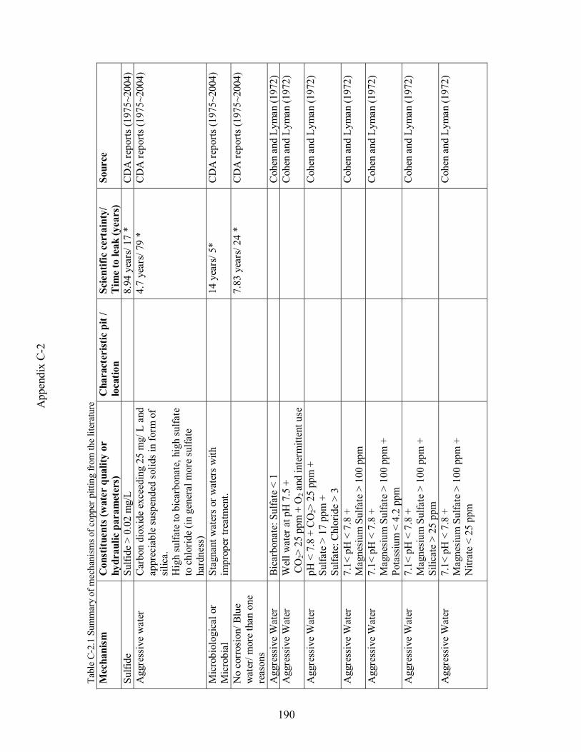
App
endi
x C
-2
Tabl
e C
-2.1
Sum
mar
y of
mec
hani
sms o
f cop
per p
ittin
g fr
om th
e lit
erat
ure
Mec
hani
sm
Con
stitu
ents
(wat
er q
ualit
y or
hy
drau
lic p
aram
eter
s)
Cha
ract
erist
ic p
it /
loca
tion
Scie
ntifi
c ce
rtai
nty/
T
ime
to le
ak (y
ears
) So
urce
Sulfi
de
Sulfi
de >
0.0
2 m
g/L
8.
94 y
ears
/ 17
* C
DA
repo
rts (1
975~
2004
) A
ggre
ssiv
e w
ater
C
arbo
n di
oxid
e ex
ceed
ing
25 m
g/ L
and
ap
prec
iabl
e su
spen
ded
solid
s in
form
of
silic
a.
Hig
h su
lfate
to b
icar
bona
te, h
igh
sulfa
te
to c
hlor
ide
(in g
ener
al m
ore
sulfa
te
hard
ness
)
4.
7 ye
ars/
79
* C
DA
repo
rts (1
975~
2004
)
Mic
robi
olog
ical
or
Mic
robi
al
Stag
nant
wat
ers o
r wat
ers w
ith
impr
oper
trea
tmen
t.
14 y
ears
/ 5*
CD
A re
ports
(197
5~20
04)
No
corr
osio
n/ B
lue
wat
er/ m
ore
than
one
re
ason
s
7.83
yea
rs/ 2
4 *
CD
A re
ports
(197
5~20
04)
Agg
ress
ive
Wat
er
Bica
rbon
ate:
Sul
fate
< 1
C
ohen
and
Lym
an (1
972)
A
ggre
ssiv
e W
ater
W
ell w
ater
at p
H 7
.5 +
C
O2>
25
ppm
+ O
2 and
inte
rmitt
ent u
se
Coh
en a
nd L
yman
(197
2)
Agg
ress
ive
Wat
er
pH <
7.8
+ C
O2>
25
ppm
+
Sulfa
te >
17
ppm
+
Sulfa
te: C
hlor
ide
> 3
Coh
en a
nd L
yman
(197
2)
Agg
ress
ive
Wat
er
7.1<
pH
< 7
.8 +
M
agne
sium
Sul
fate
> 1
00 p
pm
Coh
en a
nd L
yman
(197
2)
Agg
ress
ive
Wat
er
7.1<
pH
< 7
.8 +
M
agne
sium
Sul
fate
> 1
00 p
pm +
Po
tass
ium
< 4
.2 p
pm
Coh
en a
nd L
yman
(197
2)
Agg
ress
ive
Wat
er
7.1<
pH
< 7
.8 +
M
agne
sium
Sul
fate
> 1
00 p
pm +
Si
licat
e >
25 p
pm
Coh
en a
nd L
yman
(197
2)
Agg
ress
ive
Wat
er
7.1<
pH
< 7
.8 +
M
agne
sium
Sul
fate
> 1
00 p
pm +
N
itrat
e <
25 p
pm
Coh
en a
nd L
yman
(197
2)
190

App
endi
x C
-2
Tabl
e C
-2.1
Sum
mar
y of
mec
hani
sms o
f cop
per p
ittin
g fr
om th
e lit
erat
ure
Mec
hani
sm
Con
stitu
ents
(wat
er q
ualit
y or
hy
drau
lic p
aram
eter
s)
Cha
ract
erist
ic p
it /
loca
tion
Scie
ntifi
c ce
rtai
nty/
T
ime
to le
ak (y
ears
) So
urce
Agg
ress
ive
Wat
er
Soft
wat
er w
ith p
H <
6.5
+
10 p
pm <
CO
2 < 5
0 pp
m +
Lo
w in
chl
orid
e, su
lfate
, nitr
ate
ions
+
hot w
ater
syst
em
Coh
en a
nd L
yman
(197
2)
Agg
ress
ive
Wat
er
pH >
7.8
+ c
old
wat
er +
bi
carb
onat
e <
40 p
pm
19
.3 y
ears
/ 6 *
* C
ohen
and
Mye
rs (1
984)
Agg
ress
ive
Wat
er
pH >
7.8
+ c
old
wat
er +
bi
carb
onat
e >
54.6
ppm
+
CO
2 > 4
.8 p
pm
37
.7 y
ears
/ 9 *
* C
ohen
and
Mye
rs (1
984)
Agg
ress
ive
Wat
er
pH >
7.8
+ c
old
wat
er +
bi
carb
onat
e >
54.6
ppm
+
CO
2< 4
.8 p
pm
50
yea
rs/ 1
1 **
C
ohen
and
Mye
rs (1
984)
Agg
ress
ive
Wat
er
pH <
7.8
+ c
old
wat
er +
+
CO
2 > 2
5 pp
m +
D
issol
ved
oxyg
en >
7.8
ppm
2.
6 ye
ars/
34
**
Coh
en a
nd M
yers
(198
4)
Agg
ress
ive
Wat
er
pH <
7.8
+ c
old
wat
er +
+
CO
2 > 2
5 pp
m +
D
issol
ved
oxyg
en <
7.8
ppm
9.
4 ye
ars/
18
**
Coh
en a
nd M
yers
(198
4)
Agg
ress
ive
Wat
er
pH <
7.8
+ c
old
wat
er +
+
CO
2 < 2
5 pp
m +
Sul
fate
> 1
7 pp
m +
Su
lfate
: C
hlor
ide
> 3:
3
2.
4 ye
ars/
8 *
* C
ohen
and
Mye
rs (1
984)
Agg
ress
ive
Wat
er
pH <
7.8
+ c
old
wat
er +
+
CO
2 < 2
5 pp
m +
Sul
fate
> 1
7 pp
m +
Su
lfate
: C
hlor
ide
< 3:
3 +
Pota
ssiu
m >
5
ppm
32
.8 y
ears
/ 8 *
* C
ohen
and
Mye
rs (1
984)
Agg
ress
ive
Wat
er
pH <
7.8
+ c
old
wat
er +
+
CO
2 < 2
5 pp
m +
Sul
fate
> 1
7 pp
m +
Su
lfate
: C
hlor
ide
< 3:
3 +
Pota
ssiu
m <
4.2
ppm
+
Silic
on d
ioxi
de >
26.
2 pp
m
3.
6 ye
ars/
8 *
* C
ohen
and
Mye
rs (1
984)
191
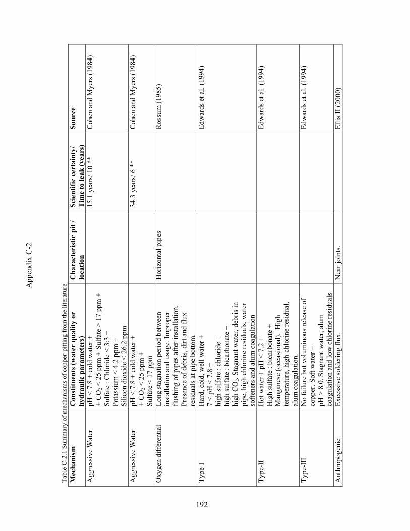
App
endi
x C
-2
Tabl
e C
-2.1
Sum
mar
y of
mec
hani
sms o
f cop
per p
ittin
g fr
om th
e lit
erat
ure
Mec
hani
sm
Con
stitu
ents
(wat
er q
ualit
y or
hy
drau
lic p
aram
eter
s)
Cha
ract
erist
ic p
it /
loca
tion
Scie
ntifi
c ce
rtai
nty/
T
ime
to le
ak (y
ears
) So
urce
Agg
ress
ive
Wat
er
pH <
7.8
+ c
old
wat
er +
+
CO
2 < 2
5 pp
m +
Sul
fate
> 1
7 pp
m +
Su
lfate
: C
hlor
ide
< 3:
3 +
Pota
ssiu
m <
4.2
ppm
+
Silic
on d
ioxi
de <
26.
2 pp
m
15
.1 y
ears
/ 10
**
Coh
en a
nd M
yers
(198
4)
Agg
ress
ive
Wat
er
pH <
7.8
+ c
old
wat
er +
+
CO
2 < 2
5 pp
m +
Su
lfate
< 1
7 pp
m
34
.3 y
ears
/ 6 *
* C
ohen
and
Mye
rs (1
984)
Oxy
gen
diff
eren
tial
Long
stag
natio
n pe
riod
betw
een
inst
alla
tion
and
usag
e. Im
prop
er
flush
ing
of p
ipes
afte
r ins
talla
tion.
Pr
esen
ce o
f deb
ris, d
irt a
nd fl
ux
resi
dual
s at p
ipe
botto
m.
Hor
izon
tal p
ipes
Ros
sum
(198
5)
Type
-I
Har
d, c
old,
wel
l wat
er +
7
< pH
< 7
.8 +
hi
gh su
lfate
: ch
lorid
e +
high
sulfa
te :
bica
rbon
ate
+ hi
gh C
O2.
Stag
nant
wat
er, d
ebris
in
pipe
, hig
h ch
lorin
e re
sidu
als,
wat
er
softe
ners
and
alu
m c
oagu
latio
n
Edw
ards
et a
l. (1
994)
Type
-II
Hot
wat
er +
pH
< 7
.2 +
H
igh
sulfa
te :
bica
rbon
ate
+
Man
gane
se (o
ccas
iona
l). H
igh
tem
pera
ture
, hig
h ch
lorin
e re
sidu
al,
alum
coa
gula
tion.
Edw
ards
et a
l. (1
994)
Type
-III
No
failu
re b
ut v
olum
inou
s rel
ease
of
copp
er. S
oft w
ater
+
pH >
8.0
. Sta
gnan
t wat
er, a
lum
co
agul
atio
n an
d lo
w c
hlor
ine
resi
dual
s
Edw
ards
et a
l. (1
994)
Ant
hrop
ogen
ic
Exce
ssiv
e so
lder
ing
flux.
N
ear j
oint
s.
Ellis
II (2
000)
192

App
endi
x C
-2
Tabl
e C
-2.1
Sum
mar
y of
mec
hani
sms o
f cop
per p
ittin
g fr
om th
e lit
erat
ure
Mec
hani
sm
Con
stitu
ents
(wat
er q
ualit
y or
hy
drau
lic p
aram
eter
s)
Cha
ract
erist
ic p
it /
loca
tion
Scie
ntifi
c ce
rtai
nty/
T
ime
to le
ak (y
ears
) So
urce
Sold
erin
g flu
x Im
prop
er o
r exc
essi
ve u
se o
f sol
derin
g flu
x, p
oor w
orkm
ansh
ip o
r Flu
xes n
ot
conf
orm
ing
to A
STM
B81
3 sta
ndar
ds.
Mye
rs a
nd C
ohen
(200
5)
Hyd
roge
n Su
lfide
Su
lfide
> 0
.02
mg/
L, o
r wel
l wat
ers
with
Sul
fate
redu
cing
bac
teria
.
M
yers
and
Coh
en (2
005)
Eros
ion
corr
osio
n V
eloc
ities
exc
eedi
ng 4
~5 fp
s or
pres
sure
exc
eedi
ng 8
0 ps
i, sh
oddy
w
orkm
ansh
ip, S
oft w
ater
with
nea
rly
zero
har
dnes
s and
wat
er c
onta
inin
g ap
prec
iabl
e am
ount
s of d
issol
ved
oxyg
en a
nd c
arbo
n di
oxid
e. (h
ot w
ater
re
circ
ulat
ion
syst
ems
wor
st im
pact
ed)
Mye
rs a
nd C
ohen
(200
5)
Cup
roso
lven
cy
Soft
wat
er w
ith n
ear z
ero
hard
ness
, pH
le
ss th
an 7
and
low
alk
alin
ity. I
n ge
nera
l due
to p
rese
nce
of C
O2.
Con
cent
ratio
n ce
ll C
orro
sion
Dep
osits
of i
ron
oxid
es a
nd/ S
ilica
/ sa
nd, p
rese
nce
of d
issol
ved
oxyg
en in
w
ater
.
Che
mist
ry re
late
d to
C
old-
wat
er p
ittin
g Lo
w p
H, h
igh
alka
linity
, wel
l wat
er o
r a
com
bina
tion
of w
ell a
nd su
rfac
e w
ater
. C
orro
sive
age
nt is
CO
2.
Che
mist
ry re
late
d to
H
ot-w
ater
pitt
ing
Pres
ence
of i
ron,
man
gane
se, a
nd/ o
r al
umin
um a
nd o
ften
silic
a co
ntai
ning
co
nstit
uent
. The
con
cent
ratio
ns re
quire
to
initi
ate
pitti
ng b
e ar
ound
0.1
mg/
L.
Hot
wat
er te
mpe
ratu
res a
bove
160
F.
Sulfi
de a
ttack
R
aw w
ater
with
sulfi
des
or S
RB
Nea
r col
onie
s of
SR
B N
early
100
%
Dr M
arc
Edw
ards
(P
erso
nal c
omm
unic
atio
ns)
Cl 2-
Al-h
igh
pH
pH>
7.8
Cl 2>
2.5
ppm
Pi
pes i
n fr
eque
nt
flow
and
at l
ocat
ions
10
0%
Dr M
arc
Edw
ards
(P
erso
nal c
omm
unic
atio
ns)
193
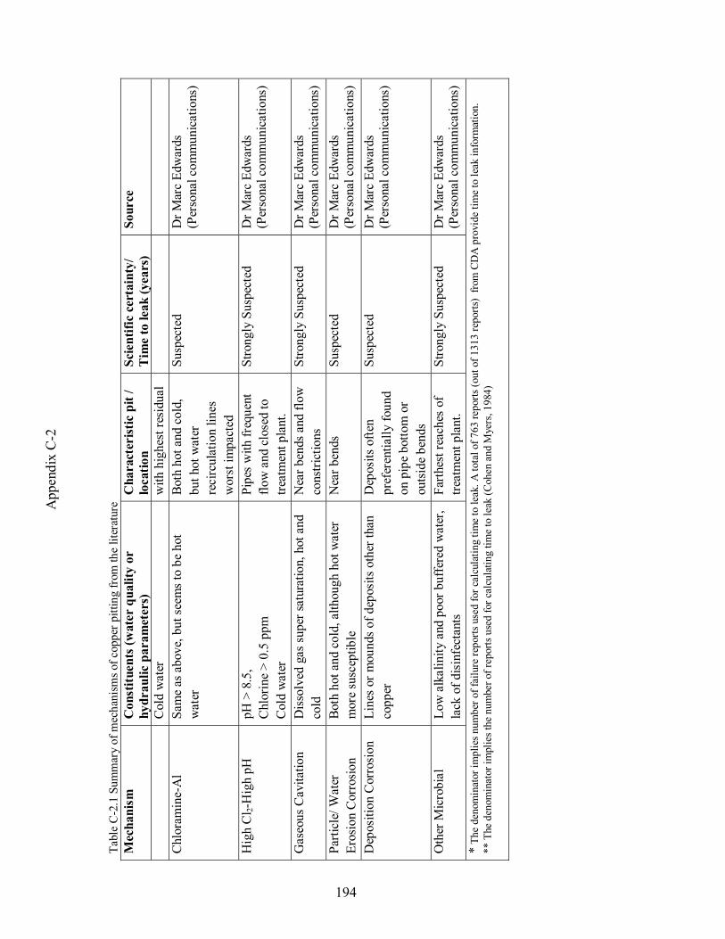
App
endi
x C
-2
Tabl
e C
-2.1
Sum
mar
y of
mec
hani
sms o
f cop
per p
ittin
g fr
om th
e lit
erat
ure
Mec
hani
sm
Con
stitu
ents
(wat
er q
ualit
y or
hy
drau
lic p
aram
eter
s)
Cha
ract
erist
ic p
it /
loca
tion
Scie
ntifi
c ce
rtai
nty/
T
ime
to le
ak (y
ears
) So
urce
Col
d w
ater
w
ith h
ighe
st re
sidu
al
Chl
oram
ine-
Al
Sam
e as
abo
ve, b
ut se
ems t
o be
hot
w
ater
Bo
th h
ot a
nd c
old,
bu
t hot
wat
er
reci
rcul
atio
n lin
es
wor
st im
pact
ed
Susp
ecte
d D
r Mar
c Ed
war
ds
(Per
sona
l com
mun
icat
ions
)
Hig
h C
l 2-H
igh
pH
pH >
8.5
, C
hlor
ine
> 0.
5 pp
m
Col
d w
ater
Pipe
s w
ith fr
eque
nt
flow
and
clo
sed
to
treat
men
t pla
nt.
Stro
ngly
Sus
pect
ed
Dr M
arc
Edw
ards
(P
erso
nal c
omm
unic
atio
ns)
Gas
eous
Cav
itatio
n D
issol
ved
gas s
uper
satu
ratio
n, h
ot a
nd
cold
N
ear b
ends
and
flow
co
nstri
ctio
ns
Stro
ngly
Sus
pect
ed
Dr M
arc
Edw
ards
(P
erso
nal c
omm
unic
atio
ns)
Parti
cle/
Wat
er
Eros
ion
Cor
rosio
n Bo
th h
ot a
nd c
old,
alth
ough
hot
wat
er
mor
e su
scep
tible
N
ear b
ends
Su
spec
ted
Dr M
arc
Edw
ards
(P
erso
nal c
omm
unic
atio
ns)
Dep
ositi
on C
orro
sion
Li
nes o
r mou
nds o
f dep
osits
oth
er th
an
copp
er
Dep
osits
ofte
n pr
efer
entia
lly fo
und
on p
ipe
botto
m o
r ou
tsid
e be
nds
Susp
ecte
d D
r Mar
c Ed
war
ds
(Per
sona
l com
mun
icat
ions
)
Oth
er M
icro
bial
Lo
w a
lkal
inity
and
poo
r buf
fere
d w
ater
, la
ck o
f dis
infe
ctan
ts
Farth
est r
each
es o
f tre
atm
ent p
lant
. St
rong
ly S
uspe
cted
D
r Mar
c Ed
war
ds
(Per
sona
l com
mun
icat
ions
) *
The
deno
min
ator
impl
ies n
umbe
r of f
ailu
re re
ports
use
d fo
r cal
cula
ting
time
to le
ak. A
tota
l of 7
63 re
ports
(out
of 1
313
repo
rts)
from
CD
A p
rovi
de ti
me
to le
ak in
form
atio
n.
** T
he d
enom
inat
or im
plie
s the
num
ber o
f rep
orts
use
d fo
r cal
cula
ting
time
to le
ak (C
ohen
and
Mye
rs, 1
984)
194

Appendix D-2
195
APPENDIX D-2
Formulation of Goal Program

Appendix D-2
196
Formulation
The formulation of linear program is presented in the following section, based on the mechanism
enlisted in Table 6.
For 1=i
The mechanism has “100 %” scientific certainty, hence 11 bS ≥
14,13,12,11,1 bXXXX ≥+++
1114,13,12,11,1 bddXXXX =+−+++ −+ (D1)
For 2=i
The mechanism has “Strongly Suspected” scientific certainty, hence 324 bSb ≤≤
33,22,21,24 bXXXb ≤++≤ (D2)
4223,22,21,2 bddXXX =+−++ −+ (D3)
3333,22,21,2 bddXXX =−+++ −+ (D4)
For 3=i
The mechanism is classified as “Strongly Suspected”, hence 334 bSb ≤≤
34,33,32,31,34 bXXXXb ≤+++≤ (D5)

Appendix D-2
197
4444,33,32,31,3 bddXXXX =+−+++ −+ (D6)
3554,33,32,31,3 bddXXXX =−++++ −+ (D7)
For 4=i
The mechanism is classified as “Suspected”, hence 546 bSb ≤≤
54,43,42,41,46 bXXXXb ≤+++≤ (D8)
6664,43,42,41,4 bddXXXX =+−+++ −+ (D9)
5774,43,42,41,4 bddXXXX =−++++ −+ (D10)
For 5=i
The mechanism is classified as “Suspected”, hence 556 bSb ≤≤
54,53,52,51,56 bXXXXb ≤+++≤ (D11)
6884,53,52,51,5 bddXXXX =+−+++ −+ (D12)
5994,53,52,51,5 bddXXXX =−++++ −+ (D13)
For 6=i
The mechanism is classified as “Suspected”, hence 566 bSb ≤≤
53,62,61,66 bXXXb ≤++≤ (D14)

Appendix D-2
198
510103,62,61,6 bddXXX =−+++ −+ (D15)
611113,62,61,6 bddXXX =+−++ −+ (D16)
For 7=i
The mechanism is classified as “Below Suspected”, hence 77 bS ≤
74,73,72,71,7 bXXXX ≤+++ (D17)
712124,73,72,71,7 bddXXXX =−++++ −+ (D18)
For 8=i
The mechanism is classified as “Below Suspected”, hence 78 bS ≤
74,83,82,81,8 bXXXX ≤+++ (D19)
713134,83,82,81,8 bddXXXX =−++++ −+ (D20)
For 9=i
The mechanism has “Strongly Suspected” scientific certainty, hence 394 bSb ≤≤
34,93,92,91,94 bXXXXb ≤+++≤ (D21)
314144,93,92,91,9 bddXXXX =−++++ −+ (D22)
415154,93,92,91,9 bddXXXX =+−+++ −+ (D23)

Appendix D-2
199
For 10=i
The mechanism is classified as “Suspected”, hence 5106 bSb ≤≤
54,103,102,101,106 bXXXXb ≤+++≤ (D24)
616164,103,102,101,10 bddXXXX =+−+++ −+ (D25)
517174,103,102,101,10 bddXXXX =−++++ −+ (D26)
For 11=i
The mechanism has “Strongly Suspected” scientific certainty, hence 3114 bSb ≤≤
34,113,112,111,114 bXXXXb ≤+++≤ (D27)
318184,113,112,111,11 bddXXXX =−++++ −+ (D28)
419194,113,112,111,11 bddXXXX =+−+++ −+ (D29)
For 12=i
The mechanism is classified as “Suspected”, hence 5126 bSb ≤≤
54,123,122,121,126 bXXXXb ≤+++≤ (D30)
521214,123,122,121,12 bddXXXX =−++++ −+ (D31)
621214,123,122,121,12 bddXXXX =+−+++ −+ (D32)
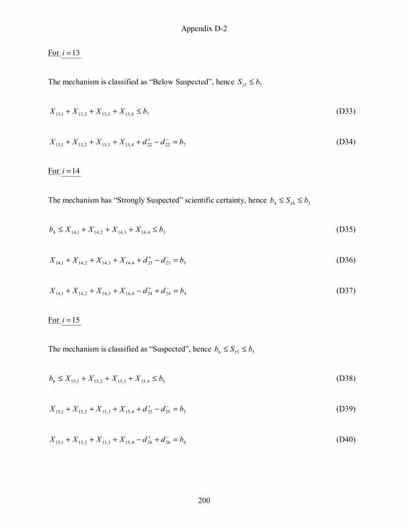
Appendix D-2
200
For 13=i
The mechanism is classified as “Below Suspected”, hence 713 bS ≤
74,133,132,131,13 bXXXX ≤+++ (D33)
722224,133,132,131,13 bddXXXX =−++++ −+ (D34)
For 14=i
The mechanism has “Strongly Suspected” scientific certainty, hence 3144 bSb ≤≤
34,143,142,141,144 bXXXXb ≤+++≤ (D35)
323234,143,142,141,14 bddXXXX =−++++ −+ (D36)
424244,143,142,141,14 bddXXXX =+−+++ −+ (D37)
For 15=i
The mechanism is classified as “Suspected”, hence 5156 bSb ≤≤
54,153,152,151,156 bXXXXb ≤+++≤ (D38)
525254,153,152,151,15 bddXXXX =−++++ −+ (D39)
626264,153,152,151,15 bddXXXX =+−+++ −+ (D40)

Appendix D-2
201
For 16=i
The mechanism is classified as “Below Suspected”, hence 716 bS ≤
73,162,161,16 bXXX ≤++ (D41)
727273,162,161,16 bddXXX =−+++ −+ (D42)
For 17=i
The mechanism is classified as “Suspected”, hence 5176 bSb ≤≤
54,173,172,171,176 bXXXXb ≤+++≤ (D43)
528284,173,172,171,17 bddXXXX =−++++ −+ (D44)
629294,173,172,171,17 bddXXXX =+−+++ −+ (D45)
For 18=i
The mechanism is classified as “Suspected”, hence 5186 bSb ≤≤
54,183,182,181,186 bXXXXb ≤+++≤ (D46)
530304,183,182,181,18 bddXXXX =−++++ −+ (D47)
631314,183,182,181,18 bddXXXX =+−+++ −+ (D48)

Appendix D-2
202
For 19=i
The mechanism is classified as “Almost 100%”, hence 11 1193 −≤≤+ bSb
11 11,193 −≤≤+ bXb (D49)
1332321,19 +=+− −+ bddX (D50)
1133331,19 −=−+ −+ bddX (D51)
For 20=i
The mechanism has “Strongly Suspected” scientific certainty, hence 3204 bSb ≤≤
34,203,202,201,204 bXXXXb ≤+++≤ (D52)
334344,203,202,201,20 bddXXXX =−++++ −+ (D53)
435354,203,202,201,20 bddXXXX =+−+++ −+ (D54)
For 21=i
The mechanism is classified as “Strongly Suspected”, hence 3214 bSb ≤≤
34,213,212,211,214 bXXXXb ≤+++≤ (D55)
336364,213,212,211,21 bddXXXX =−++++ −+ (D56)
437374,213,212,211,21 bddXXXX =+−+++ −+ (D57)

Appendix D-2
203
For 22=i
The mechanism is classified as “Suspected”, hence 5226 bSb ≤≤
54,223,222,221,226 bXXXXb ≤+++≤ (D58)
538384,223,222,221,22 bddXXXX =−++++ −+ (D59)
639394,223,222,221,22 bddXXXX =+−+++ −+ (D60)
For 23=i
The mechanism is classified as “Suspected”, hence 5236 bSb ≤≤
53,232,231,236 bXXXb ≤++≤ (D61)
540403,232,231,23 bddXXX =−+++ −+ (D62)
641413,232,231,23 bddXXX =+−++ −+ (D63)
For 24=i
The mechanism is classified as “Suspected”, hence 5246 bSb ≤≤
53,242,241,246 bXXXb ≤++≤ (D64)
542423,242,241,24 bddXXX =−+++ −+ (D65)
643433,242,241,24 bddXXX =+−++ −+ (D66)
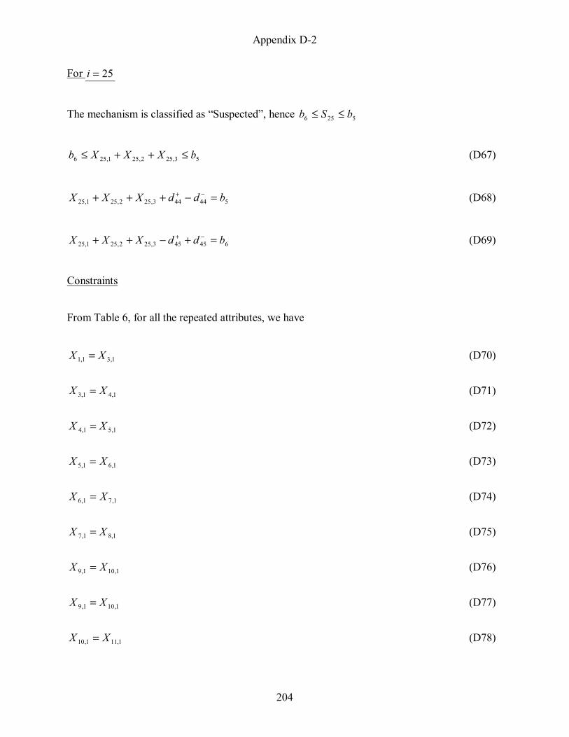
Appendix D-2
204
For 25=i
The mechanism is classified as “Suspected”, hence 5256 bSb ≤≤
53,252,251,256 bXXXb ≤++≤ (D67)
544443,252,251,25 bddXXX =−+++ −+ (D68)
645453,252,251,25 bddXXX =+−++ −+ (D69)
Constraints
From Table 6, for all the repeated attributes, we have
1,31,1 XX = (D70)
1,41,3 XX = (D71)
1,51,4 XX = (D72)
1,61,5 XX = (D73)
1,71,6 XX = (D74)
1,81,7 XX = (D75)
1,101,9 XX = (D76)
1,101,9 XX = (D77)
1,111,10 XX = (D78)

Appendix D-2
205
1,121,11 XX = (D79)
1,131,12 XX = (D80)
1,141,13 XX = (D81)
1,151,14 XX = (D82)
1,161,15 XX = (D83)
1,181,17 XX = (D84)
1,251,24 XX = (D85)
2,22,1 XX = (D86)
2,52,2 XX = (D87)
2,62,5 XX = (D88)
2,72,6 XX = (D89)
2,82,7 XX = (D90)
2,92,8 XX = (D91)
2,102,9 XX = (D92)
2,112,10 XX = (D93)
2,132,11 XX = (D94)
2,142,13 XX = (D95)

Appendix D-2
206
2,152,14 XX = (D96)
2,162,15 XX = (D97)
2,182,16 XX = (D98)
2,212,18 XX = (D99)
2,222,21 XX = (D100)
2,232,22 XX = (D101)
2,202,3 XX = (D102)
2,242,20 XX = (D103)
2,252,24 XX = (D104)
2,122,4 XX = (D105)
2,172,12 XX = (D106)
3,43,3 XX = (D107)
3,53,4 XX = (D108)
3,103,9 XX = (D109)
3,123,11 XX = (D110)
3,133,12 XX = (D111)
3,143,13 XX = (D112)
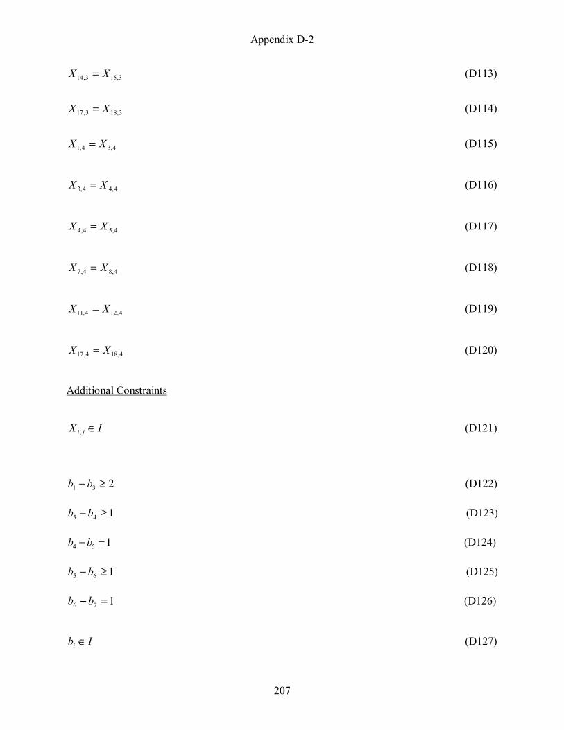
Appendix D-2
207
3,153,14 XX = (D113)
3,183,17 XX = (D114)
4,34,1 XX = (D115)
4,44,3 XX = (D116)
4,54,4 XX = (D117)
4,84,7 XX = (D118)
4,124,11 XX = (D119)
4,184,17 XX = (D120)
Additional Constraints
IX ji ∈, (D121)
231 ≥− bb (D122)
143 ≥− bb (D123)
154 =− bb (D124)
165 ≥− bb (D125)
176 =− bb (D126)
Ibi ∈ (D127)
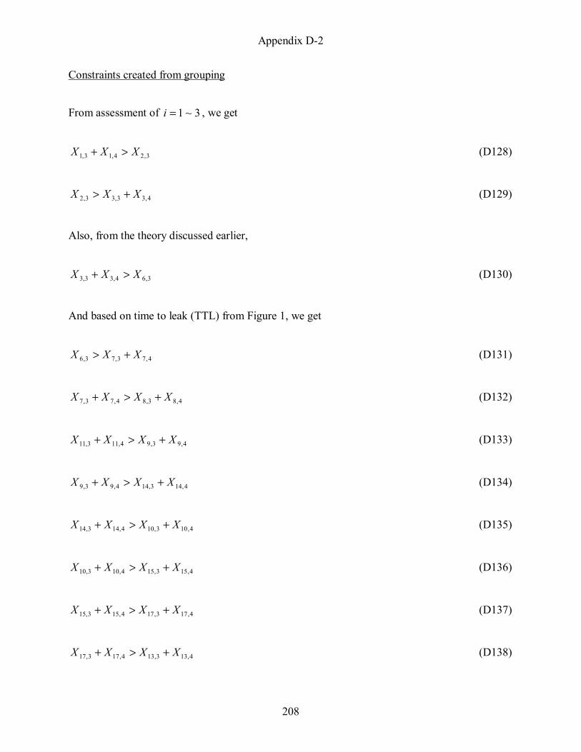
Appendix D-2
208
Constraints created from grouping
From assessment of 3~1=i , we get
3,24,13,1 XXX >+ (D128)
4,33,33,2 XXX +> (D129)
Also, from the theory discussed earlier,
3,64,33,3 XXX >+ (D130)
And based on time to leak (TTL) from Figure 1, we get
4,73,73,6 XXX +> (D131)
4,83,84,73,7 XXXX +>+ (D132)
4,93,94,113,11 XXXX +>+ (D133)
4,143,144,93,9 XXXX +>+ (D134)
4,103,104,143,14 XXXX +>+ (D135)
4,153,154,103,10 XXXX +>+ (D136)
4,173,174,153,15 XXXX +>+ (D137)
4,133,134,173,17 XXXX +>+ (D138)
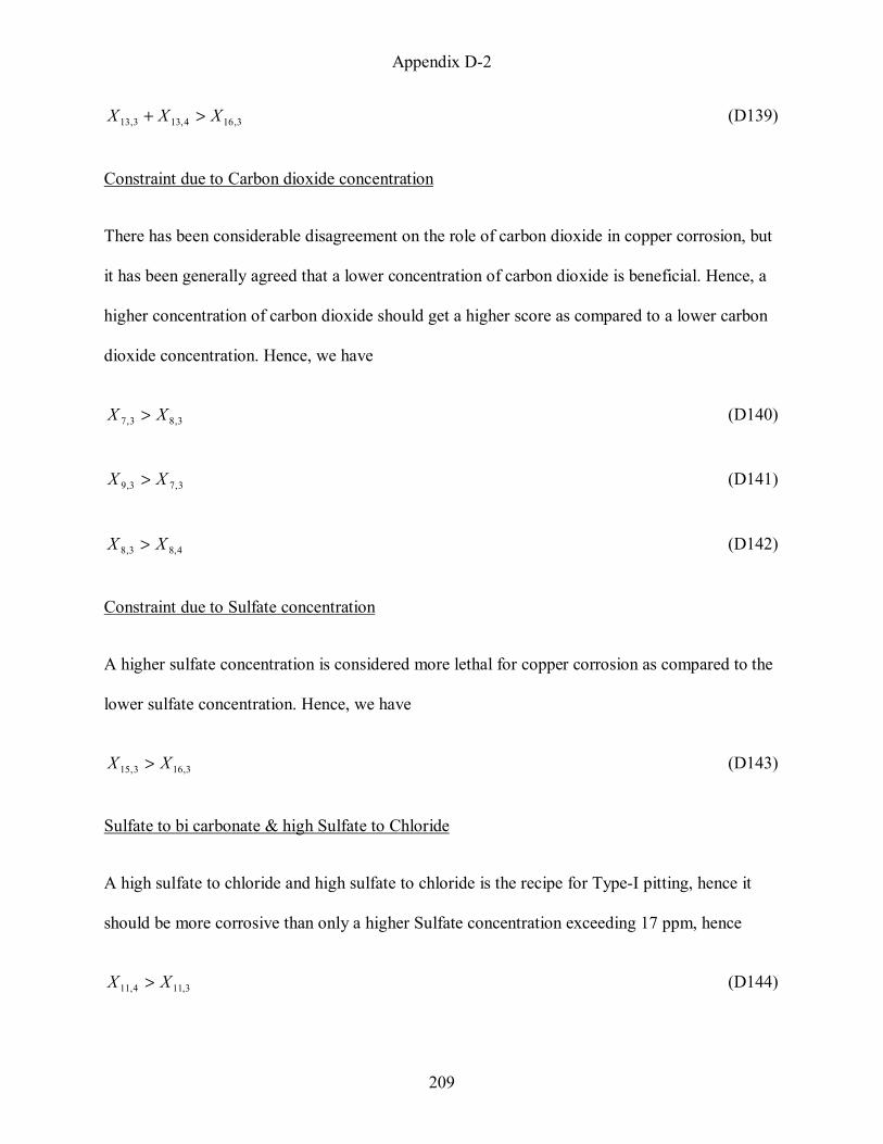
Appendix D-2
209
3,164,133,13 XXX >+ (D139)
Constraint due to Carbon dioxide concentration
There has been considerable disagreement on the role of carbon dioxide in copper corrosion, but
it has been generally agreed that a lower concentration of carbon dioxide is beneficial. Hence, a
higher concentration of carbon dioxide should get a higher score as compared to a lower carbon
dioxide concentration. Hence, we have
3,83,7 XX > (D140)
3,73,9 XX > (D141)
4,83,8 XX > (D142)
Constraint due to Sulfate concentration
A higher sulfate concentration is considered more lethal for copper corrosion as compared to the
lower sulfate concentration. Hence, we have
3,163,15 XX > (D143)
Sulfate to bi carbonate & high Sulfate to Chloride
A high sulfate to chloride and high sulfate to chloride is the recipe for Type-I pitting, hence it
should be more corrosive than only a higher Sulfate concentration exceeding 17 ppm, hence
3,114,11 XX > (D144)

Appendix D-2
210
4,143,14 XX > (D145)
4,153,15 XX > (D146)
4,173,17 XX > (D147)
Constraint due to Chlorine concentration
Higher chlorine should be more corrosive, hence
3,23,1 XX > (D148)
Also the Aluminum is suppose to act in synergy with chlorine and chloramines, and by itself
Aluminum does not have any deleterious effects. Hence,
4,13,1 XX > (D149)
4,33,3 XX > (D150)
Constraint due to DO concentration
Dissolved oxygen plays an important role in pitting initiation and propagation. A higher DO
concentration should get a higher score than a lower DO concentration. Hence, we have
3,233,21 XX > (D151)

Appendix D-2
211
Constraint due to Stagnation of water
Stagnation of water causes many problems including microbial growth, cuprosolvency etc,
however, the initial period of stagnation (between installation and usage) is considered as more
crucial with respect to corrosion (Rossum, 1985). Hence, we get
4,204,22 XX > (D152)
Other Constraints (hierarchy in attributes not pH dependant)
Excessive Soldering Flux > Low alkalinity > Pressure drop below V.P. >
> Pressure above 80 psi > Deposits of aluminum / iron
Hence
1,201,22 XX > (D153)
1,211,20 XX > (D154)
1,241,21 XX > (D155)
1,231,24 XX > (D156)
0, >jiX (D157)

212
CHAPTER-3
PROBABILISTIC MODEL FOR REPLACEMENT OF PLUMBING PIPES
As discussed in the previous chapter, the occurrence of pinhole leaks in the home
plumbing systems is dependent on synergy between physical, chemical, biological and
anthropogenic parameters. The synergy between these parameters is not completely understood
due to absence of a unified mechanistic theory, and hence to date any preventive measure for
pitting corrosion could not be ascertained. It is perceived that once pinhole leaks arrive in a
particular plumbing system, the system becomes prone to more leaks in future (WSSC data). The
decision of the homeowner to repair or replace is dependent on leak frequency, cost, previous
experience, personal perception of leak pattern willingness to pay, willingness to take risk and
personal comfort.
Figure 1 Variation of failure rate with age- a typical bath tub curve
Burn-in- period Useful life period Wear out period
Age of the system
Lea
k r
ate

213
The home plumbing systems are repairable systems; hence the variation in the failure rate
with age of these systems can be approximated using a bath tub curve, shown in Figure 1. The
life span of a typical home plumbing system can be divided into three phases based on the bath
tub curve. The three phases are distinguished based on the rate of occurrence of failure
(ROCOF), which is same as the leak rate or the failure rate.
The leak rate in the first phase or the burn in phase decreases from a higher value, the
higher value in the initial stages of the life span can be due to the poor workmanship or small
manufacturing defects in the pipes. Once these defects are rectified the leak rates in the system
should stabilize to a lower value. The second phase or the useful life period is marked by a slow
increase in the leak rates. In the event of pinhole leaks, it is perceived that the system deviates
from the normal behavior and hence the useful life period is shortened considerably. The third
phase or the wear out period is marked by a sudden increase in the leak rates, which keeps
increasing with time; this is due to the wear and tear in the system because of its aging. Since the
rate of failure is large in the third phase, it is generally beneficial to opt for a replacement during
this phase. However, the point of optimal replacement should be based on some threshold value
of the rate of failure or the leak rate.
The leak rate is a function of the inter event time and the number of leaks over a given
period of time. If consecutive leaks are considered then the leak rate shall only be a function of
the inter event time. Hence, from a home owners perspective the replacement of the system
should be dependent on the inter event time of the consecutive leaks. This is a valid assumption,
as in the event of a decreased inter event time or frequent leaks the homeowner would

214
necessarily opt for an early replacement, similarly if the inter event time is large, the decision of
the homeowner would be more inclined towards a repair rather than replacing the whole
plumbing system. Hence, the threshold value of the inter event time is essential for a homeowner
to decide the course of action in the event of a leak.
Interestingly, the information about the threshold leak rates is necessary but not a
sufficient condition from decision making perspective. For instance, in the event of a nth leak, the
homeowner would know the inter event time between the nth and (n-1)th leak, however this inter
event time when compared to the threshold inter event time, will only validate the homeowner’s
decision that was taken at the time of (n-1)th leak, thus making the decision a post facto event.
Hence, it is imperative that the inter event time between the nth and the (n+1)th leak should be
known ahead of time, specifically at the time of nth failure or before. This necessitates the need
of the probabilistic model that can pinpoint the nth leak after which the system should be
replaced.
It follows from the above discussion that from decision making perspective, the two
essential parameters are the threshold value of the inter event time and the point on the time line
at which this threshold value is reached. In order to account for the above requirements, the
model should capture the variability of the leak rate with time. Assuming, the bath tub curve to
be valid, the leak rates in the plumbing systems are expected to increase with age of the
plumbing system. Thus the leak rate curve (as called from now on) becomes the essence of the
probabilistic model.

215
The sections are organized as follows. First the available databases are discussed. Second
the model building approach is discussed along with the assumptions, methodology and
simulations. Third the simulation results are used to obtain optimal replacement criterion for
plumbing systems.
Available Data
The databases that provide information about the temporal distribution of leaks are
discussed. The data obtained from these sources is presented and the strength and the weaknesses
of each database are discussed.
CDA database
The description and analysis protocol followed by Copper Development Association
(CDA) was presented in chapter-1. The CDA failure reports typically provide information about
the installation year of the plumbing system from which the failure specimen was withdrawn.
Many of the CDA reports also furnish information about the year and month of the first leak.
A total of 763 CDA reports analyzed for this study contain the information about the
installation year and the year of the first leak. The database does not provide any specific
information about the inter event time of the subsequent leaks. The information provided in the
CDA database is used to obtain the time to first leak distribution. Any other inference related to
the leak rate curve could not be obtained from the database.

216
The time to first leak data for cold and hot water pipes is presented in the following
section. The time to first leak was calculated by taking the difference between the first leak year
and the installation year. The distribution of time to first leak for cold water and hot pipes are
shown in Figure 2. The descriptive statistics are presented in Table 1. On an average, the cold
water pipes have a smaller time to first leak as compared to hot water pipes, this is supported by
the fact that hot water pipes are protected by formation of calcium carbonate scale, which does
not form in cold water pipes unless the water is lime softened and saturated with carbonate ions.
0
10
20
30
40
50
60
70
80
90
100
0 3 6 9 12 15 18 21 24 27 30 33 36 39 42 45 48
Time to first leak (years)
Freq
uenc
y
Figure 2 Frequency distribution for time to first leak in hot water and cold water pipes from CDA data
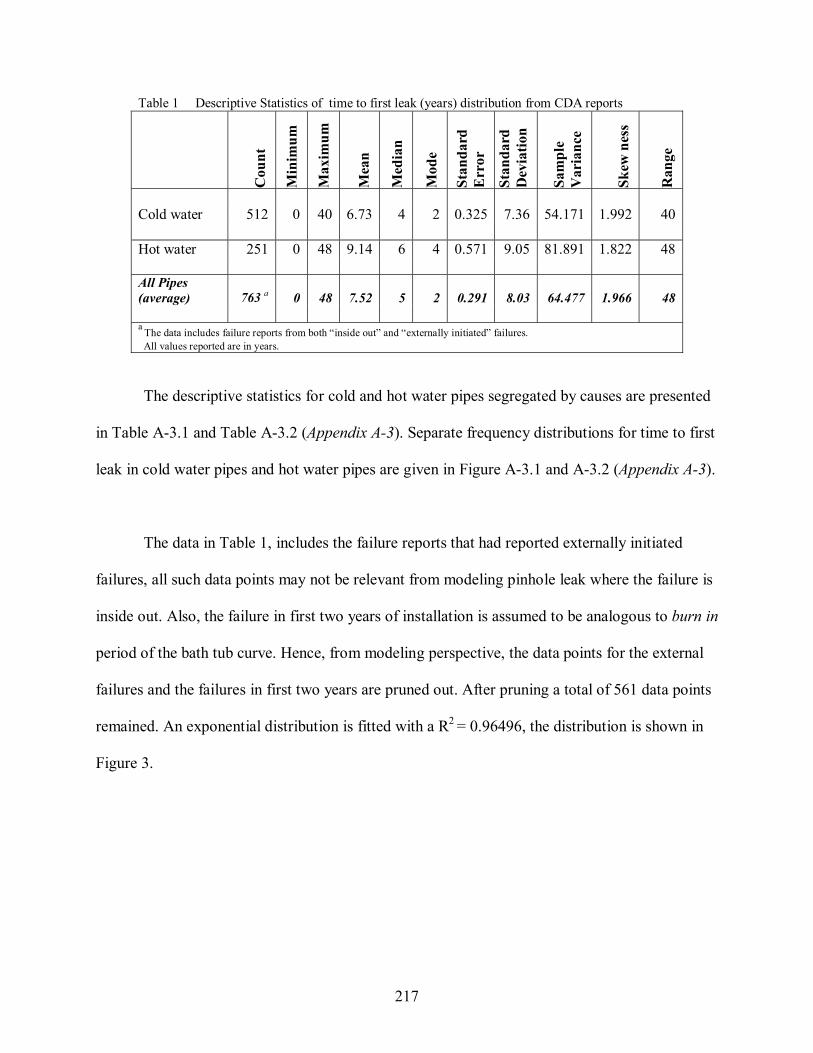
217
Table 1 Descriptive Statistics of time to first leak (years) distribution from CDA reports
Cou
nt
Min
imum
Max
imum
Mea
n
Med
ian
Mod
e
Stan
dard
E
rror
Stan
dard
D
evia
tion
Sam
ple
Var
ianc
e
Skew
nes
s
Ran
ge
Cold water 512 0 40 6.73 4 2 0.325 7.36 54.171 1.992 40 Hot water 251 0 48 9.14 6 4 0.571 9.05 81.891 1.822 48 All Pipes (average) 763 a 0 48 7.52 5 2 0.291 8.03 64.477 1.966 48 a The data includes failure reports from both “inside out” and “externally initiated” failures. All values reported are in years.
The descriptive statistics for cold and hot water pipes segregated by causes are presented
in Table A-3.1 and Table A-3.2 (Appendix A-3). Separate frequency distributions for time to first
leak in cold water pipes and hot water pipes are given in Figure A-3.1 and A-3.2 (Appendix A-3).
The data in Table 1, includes the failure reports that had reported externally initiated
failures, all such data points may not be relevant from modeling pinhole leak where the failure is
inside out. Also, the failure in first two years of installation is assumed to be analogous to burn in
period of the bath tub curve. Hence, from modeling perspective, the data points for the external
failures and the failures in first two years are pruned out. After pruning a total of 561 data points
remained. An exponential distribution is fitted with a R2 = 0.96496, the distribution is shown in
Figure 3.

218
0
0.02
0.04
0.06
0.08
0.1
0.12
0.14
0.16
0 4 8 12 16 20 24 28 32 36 40 44 48
Time (Years)
Rela
tive
Freq
uenc
y De
nsity
Relative Frequency Density Fitted Exponential (Mean=9.06)
Figure 3 Fitted Exponential distribution for time to first leak.
The exponential distribution is not a strong fit, but due to significant noise in the middle
portion of the data, the fit did not improve with truncation of data or even with other
distributions. Due to this reason, the standard deviation of the fitted exponential distribution
( 06.7=fitσ ) does not match very well with the standard deviation of the data set ( 16.8=dataσ ).
The descriptive statistics of the data after pruning is given in Table A-3.3. The curve fitting
calculations are shown in Table A-3.4.
Since the data is based on failures that were reported from different parts across the
nation it closely represents the pattern of first leak time throughout the nation. The data is not
location specific; hence the variability of the leak patterns due to change in climatic conditions,
water quality, usage patterns, and other demographic aspects is well knitted within the data. The

219
CDA database does not provide any information about the subsequent leaks or their temporal
distribution; hence from model building perspective the information is incomplete.
WSSC database
The Washington Suburban Sanitary Commission (WSSC) advises its costumers to report
the pinhole incidents on http://www.wssc.dst.md.us/copperpipe/pipeleakhomepage.cfm . The
homeowners are required to answer a questionnaire for reporting pinhole leaks. This web based
data accumulation technique keeps the data continuously updated in a dynamic fashion. For the
present study the data obtained in the year 2003 is discussed. The data is based on the pinhole
failures in about 4500 homes in the area serviced by WSSC. The data provides information about
the year of installation, year and month of first leak, total number of leaks and the year of last
leak reported for these 4500 homes. There were some errors in the original data set; the errors
included the inconsistency in reporting the years of installation and first leak in proper
chronology, missing digits of year of installation etc. After omitting these errors and
inconsistencies a total of 3786 data points remained for analysis.
The time of first leak was obtained by taking the difference between the year of first leak
and the year of installation. The distribution for time to first leak from WSSC data is presented in
Figure 4.
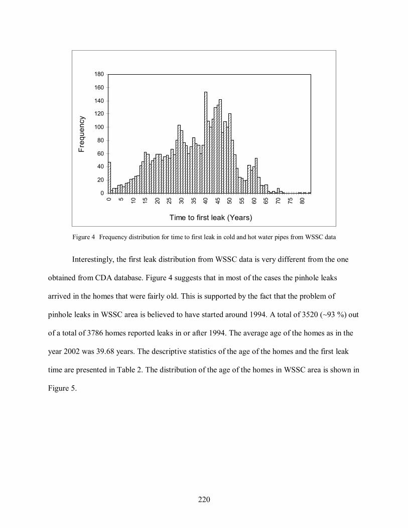
220
0
20
40
60
80
100
120
140
160
180
0 5 10 15 20 25 30 35 40 45 50 55 60 65 70 75 80
Time to first leak (Years)
Freq
uenc
y
Figure 4 Frequency distribution for time to first leak in cold and hot water pipes from WSSC data
Interestingly, the first leak distribution from WSSC data is very different from the one
obtained from CDA database. Figure 4 suggests that in most of the cases the pinhole leaks
arrived in the homes that were fairly old. This is supported by the fact that the problem of
pinhole leaks in WSSC area is believed to have started around 1994. A total of 3520 (~93 %) out
of a total of 3786 homes reported leaks in or after 1994. The average age of the homes as in the
year 2002 was 39.68 years. The descriptive statistics of the age of the homes and the first leak
time are presented in Table 2. The distribution of the age of the homes in WSSC area is shown in
Figure 5.

221
0
0.01
0.02
0.03
0.04
0.05
0.06
0.07
0.08
0 4 8 12 16 20 24 28 32 36 40 44 48 52 56 60 64 68 72
Age
Rel
ativ
e Fr
eque
ncy
Figure 5 Relative Frequency distribution for the age of homes in WSSC area.
Table 2 Descriptive Statistics of the time to first leak and age of homes distribution from WSSC data
Cou
nt
Min
imum
Max
imum
Mea
n
Med
ian
Mod
e
Stan
dard
E
rror
Stan
dard
D
evia
tion
Sam
ple
Var
ianc
e
Skew
nes
s
Ran
ge
Age of homes 3786 1 97 39.68 42 52 0.231 14.18 201.2 -0.26 96 Time to first leak 3786 0 95 36.05 38 40 0.236 14.57 212.2 -0.28 95 All values reported are in years.
From the analysis of the age of the homes in WSSC area, it becomes clear that
around 1994 there was a sudden increase in the pinhole leak incidents in the WSSC area, due to
which the first leak arrived in majority of older homes that were leak free before that period. Due
to this reason the first leak distribution is skewed to the left (Figure 4). The WSSC data captures
the period of maximum intensity of pinhole leaks for a specific location or region, and hence a
comparison with CDA data is not very justified.

222
The WSSC data also provides information about total number of leaks in the homes and
the date of the occurrence of the last leak. Based on this information, the average leak rate was
calculated. Following expression was used for the average leak rate calculation
Average leak rate
= Total number of leaks ÷ Last leak year – First leak year + 1 (1)
The homes were grouped by age in a ten year interval and the averaged value for each group was
calculated. The variation of leak rates with age of the homes is shown in Figure 6.
0.00
0.50
1.00
1.50
2.00
2.50
Age (Yrs)
Aver
age
num
ber o
f lea
ks
per y
ear p
er h
ouse
1.87 1.78 1.56 1.47 1.54 1.55 1.57 2.15 2.05
5 15 25 35 45 55 65 75 85
Figure 6 Average leak rates distribution with age of homes in WSSC area.
It may be concluded that the pinhole incidents struck the WSSC area when the houses in
the region were fairly old. It is possible that most of these houses would have already entered in
the wear out period, considering the bath tub curve. Hence, the leak incidents became severe
within a small time period. Due to this reason, the first leak time and the leak rates obtained are

223
much higher. Hence, the data from WSSC area represents the failures that would occur under the
most severe combination. Additionally, the WSSC data is not a true representative of the nation
wide pinhole leak occurrence, as it pertains to a specific location in comparison to CDA data.
From model building perspective, the data may not be used directly and may require additional
pruning or alterations in leak rates. Any model based on the WSSC data may not be very useful
for other areas, as the leak rates obtained from WSSC data are high.
Homeowner Survey
The homeowner survey, conducted by Virgina Tech Survey Research Center, consists of
leak time information from 83 respondents, who reported to have experienced pinhole leaks in
their homes. However, out of 83 respondents, 45 reported to have copper pipes in their home
plumbing. There is a slight discrepancy in the survey data, as some of the respondents who
reported to have pipes other than copper in their plumbing, later reported copper as the material
in which the failure occurred, while some of the respondents who chose copper as the material in
their plumbing later chose other material in which the failure occurred. For the purpose of this
study, only the 45 respondents that reported copper as their plumbing material were considered.
Out of 45 data points available from the survey, 6 respondents did not provide the year of
installation or the year or first leak or both. Hence, a total of 39 data points remained for
analysis.
Out of these 39 respondents, 10 were from an unnamed community in Florida, 6 from an
unnamed community in Ohio, 5 from California and 18 were from rest of United States. The two

224
unnamed communities in Florida and Ohio were previously identified as hotspots. The time to
first leak distribution from the homeowner survey data is presented in Figure 7.
0
0.5
1
1.5
2
2.5
3
3.5
4
4.5
1 6 11 16 21 26 31 36 41 46 51 56 61 66
Time to first leak (years)
Freq
uenc
y
Figure 7 Frequency distribution for time to first leak from homeowner survey data
As such the time to first leak from the survey does not show any specific pattern and is
sparse. This may be because of lack of sufficient data points for the analysis. Hence, no
conclusion about the pattern of the first leak time could be made from the survey results.
Based on the information about the subsequent leaks, the leak rates were calculated from
the survey by grouping houses in different age groups. A 10 year time interval was adopted for
grouping the houses, the leak rates calculated were averaged for each group. The variation of
leak rates with the age is presented in Figure 8.

225
0.00
0.50
1.00
1.50
2.00
2.50
3.00
3.50
4.00
4.50
Age (yrs)
Ave
rage
num
ber o
f Lea
kspe
r yea
r per
hou
se
0.75 3.00 0.67 1.36 3.88 0.59 0.24
5 15 25 35 45 55 65
Figure 8 Average leak rates distribution with age of homes from homeowner survey.
It may be concluded that the information from the survey is limited, due to which no
inference about the leak rates or the first leak time could be made. The data however is obtained
from a nationwide survey and it contains information from some of the hotspots namely,
unnamed communities in Florida and Ohio and parts of California, but because of its limited
number of data points it may be assumed that it is partially representative of the pinhole leak
patterns across the nation.
The Model
The basis of the model development is the bath tub curve that assumes an increase in the
leak rate with age. From a model building perspective, the first two years of the plumbing are not
considered, as it is assumed that this period is the burn in period, wherein failures related to poor
workmanship or manufacturing defects in pipes may occur. The period of two years was chosen
based on the time to first leak distribution from CDA data base. Hence, it is assume that the first

226
two year of the plumbing system should be otherwise leak free, if the burn in effect does not
come in play.
Since the leak rate varies with age of the plumbing, the leak rate is non stationary with
time. In similar work a Non Homogeneous Poisson Process was used by Loganathan and Lee,
(2005). In the paper, the leak rate curve was obtained using neural networks based on WSSC
data. The methodology of building the model is quite similar to the one adopted by Loganathan
and Lee, (2005), however, instead of using the WSSC data, the data from homeowner survey and
the CDA database is used. The methodology used in the present study is explained in the
following section.
The WSSC data is not considered for model building, as it is perceived that the data
captures the extreme circumstances, wherein older homes where subjected to a sudden attack of
pinhole leaks. It is very likely that due to this reason Loganathan and Lee, (2005) used a neural
network approach with WSSC data. It follows that the situation in WSSC area was extreme and
limited to a particular region; hence it is felt that a model based on WSSC data may not be
suitable for use in other areas. In order to build a model that can be used on a nationwide basis,
the data for the model should be based on surveys or databases wherein it has some intrinsic
character of the leak patterns from different locations. Hence, the homeowner survey along with
CDA database is chosen for the model building purposes.
The homeowner survey provides the leak patterns based on the nationwide survey,
although due to lack of sufficient number of data points, the leak rate curve obtained from the

227
survey does not provide a pattern suitable for model building. In order to use the data for the
model, suitable pruning is required to obtain an increasing leak rate curve with the age. The
pruning of data necessarily requires chopping the higher leak rates for each age group. Due to
these exclusions, the number of data points would be reduced further. In order to obtain a
reasonable leak rate curve for the model a different approach is used.
The pruned leak rates obtain from homeowner survey are initially used for NHPP
simulations, the first leak distribution obtained from the simulations is then calibrated using the
CDA time to first leak distribution, in an iterative environment by allowing the leak rate curve to
change. This approach provides a leak rate curve at the end of calibration. The secondary
advantage with the approach is that it ties the CDA time to first leak with the model, thus adding
a nationwide flavor in the simulation results. The following steps are elaborated further.
Data pruning
The objective of data pruning is to obtain an increasing leak rate curve for the model.
However, since the data used in NHPP simulations will be later calibrated, the pruned data is
subjected to change with the calibration. For pruning the data, the upper limits for each age
group was considered. The upper limit for the age group is based upon the hypothesis that for a
particular age group the leak rates beyond a certain value will be unreasonable from
homeowner’s perspective.
For instance, in the event of a leak the worst sequence of event can be perceived as
follows. The homeowner would notice stains or water marks on walls, ceilings or floor that
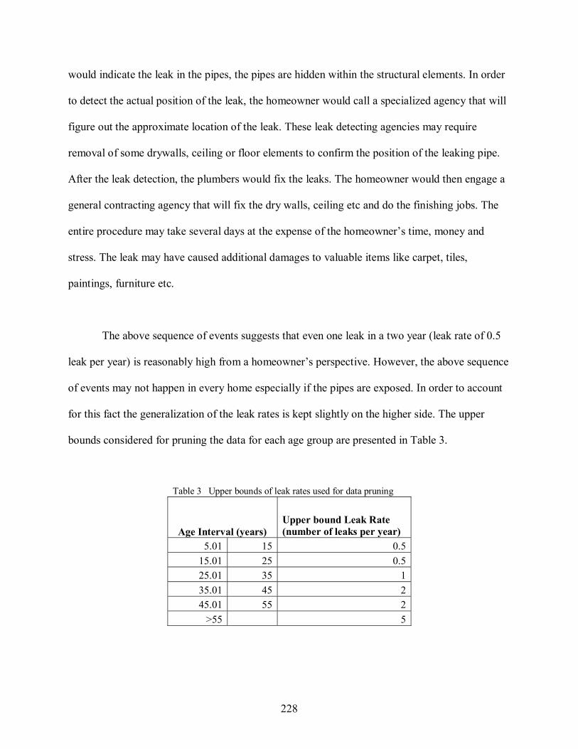
228
would indicate the leak in the pipes, the pipes are hidden within the structural elements. In order
to detect the actual position of the leak, the homeowner would call a specialized agency that will
figure out the approximate location of the leak. These leak detecting agencies may require
removal of some drywalls, ceiling or floor elements to confirm the position of the leaking pipe.
After the leak detection, the plumbers would fix the leaks. The homeowner would then engage a
general contracting agency that will fix the dry walls, ceiling etc and do the finishing jobs. The
entire procedure may take several days at the expense of the homeowner’s time, money and
stress. The leak may have caused additional damages to valuable items like carpet, tiles,
paintings, furniture etc.
The above sequence of events suggests that even one leak in a two year (leak rate of 0.5
leak per year) is reasonably high from a homeowner’s perspective. However, the above sequence
of events may not happen in every home especially if the pipes are exposed. In order to account
for this fact the generalization of the leak rates is kept slightly on the higher side. The upper
bounds considered for pruning the data for each age group are presented in Table 3.
Table 3 Upper bounds of leak rates used for data pruning
Age Interval (years) Upper bound Leak Rate (number of leaks per year)
5.01 15 0.5 15.01 25 0.5 25.01 35 1 35.01 45 2 45.01 55 2
>55 5
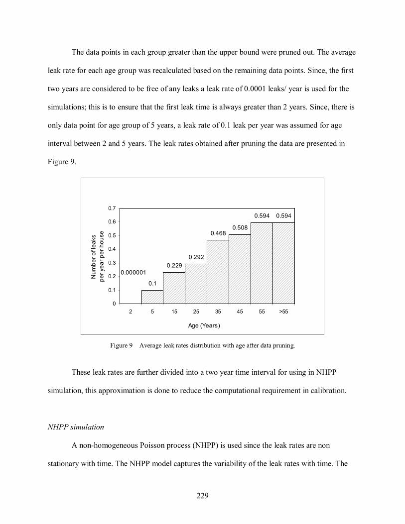
229
The data points in each group greater than the upper bound were pruned out. The average
leak rate for each age group was recalculated based on the remaining data points. Since, the first
two years are considered to be free of any leaks a leak rate of 0.0001 leaks/ year is used for the
simulations; this is to ensure that the first leak time is always greater than 2 years. Since, there is
only data point for age group of 5 years, a leak rate of 0.1 leak per year was assumed for age
interval between 2 and 5 years. The leak rates obtained after pruning the data are presented in
Figure 9.
0.1
0.2290.292
0.4680.508
0.594 0.594
0.000001
0
0.1
0.2
0.3
0.4
0.5
0.6
0.7
2 5 15 25 35 45 55 >55
Age (Years)
Num
ber o
f lea
ks
per y
ear p
er h
ouse
Figure 9 Average leak rates distribution with age after data pruning.
These leak rates are further divided into a two year time interval for using in NHPP
simulation, this approximation is done to reduce the computational requirement in calibration.
NHPP simulation
A non-homogeneous Poisson process (NHPP) is used since the leak rates are non
stationary with time. The NHPP model captures the variability of the leak rates with time. The

230
model was used for defining optimal replacement criteria based on minimum cost by Loganathan
and Lee, (2005). According to the NHPP process, if the counting of failure is started at 0=t ,
then the number of leaks ( )1TN in the time interval 10 Tt ≤≤ is defined by,
( ) ( )dttTNT
∫=1
01 λ (2)
The total number of leaks ( )2TN at the end of another time interval, such that 21 TtT ≤≤ , will be
the sum of the number of leaks in the time interval 10 Tt ≤≤ and the number of leaks in the
second time interval, hence,
( ) ( ) ( )dttTNTNT
T∫+=2
1
12 λ
Or
( ) ( ) ( )dttTNTNT
T∫=−2
1
12 λ (3)
The stepwise approach used to perform NHPP simulation is presented, a sample calculation for
the simulation is shown in Table 4. The approach for the simulation is same as used by
Loganathan and Lee, (2005).
The maximum leak rate is chosen for generation a time stationary Poisson process.
Hence, ( ) tλλ max= . The inter event time is assumed to be exponential, with the
parameter λ . Hence, for the exponentially distributed inter event time iy , for any leak to
arrive within x ,

231
( ) xx
y edyexF λλλ −− −== ∫ 10
. (4)
Since 1)(0 ≤≤ xF , it is substituted by a uniform random number ( )1,0U (refer Col. 1 of
Table 4). It follows from above,
( )Ux −
−= 1ln1
λ (5)
Since, x is the inter event time, it will be added to the previous time to get the leak time,
hence,
11 ++ += iii xtt (6)
Following Loganathan and Lee, (2005) and Ross, (2000), any event that occurs at any
time t as NHPP with parameter ( )tλ , shall be equivalent to the event that occurred as a
homogenous Poisson with a parameter λ and probability not exceeding ( )λ
λ t . Hence,
for each value of it the corresponding ( )tλ value is obtained from the leak rate curve
(Col. 5).
The leak ratio is calculated using the parameterλ , for each ( )tλ value (Col. 6). For the
probability comparison, a uniform random number is generated ( )1,0U (Col. 7).
The leak is counted if ( )λ
λ tU i ≤ , else the same is discarded for counting purposes
(Col. 8).

232
The simulation was repeated 600 times, the entire simulation was set up in a spread sheet
that enabled the calibration of the ( )tλ values in the next step. The leak times obtained from this
step are for un-calibrated values of the leak rates, these leak rates are the same as presented
earlier in Figure 9.
Table 4 Sample calculations for NHPP simulations Col. 1 Col. 2 Col. 3 Col. 4 Col. 5 Col. 6 Col. 7 Col.8
U(0,1) 1-U(0,1) X =
(1/ λ )Ln(1-U) Leak time
Leak rate Ratio U(0,1) NHPP
0.0212 0.9788 0.0361 0.0361 0.0000 0.0000 0.1667 -9999 0.2275 0.7725 0.4348 0.4709 0.0000 0.0000 0.6796 -9999 0.5402 0.4598 1.3085 1.7794 0.0000 0.0000 0.4467 -9999 0.3472 0.6528 0.7182 2.4977 0.1000 0.1684 0.0293 2.498 0.6016 0.3984 1.5499 4.0476 0.1000 0.1684 0.2217 -9999 0.2714 0.7286 0.5332 4.5808 0.1000 0.1684 0.1278 4.581 0.8355 0.1645 3.0395 7.6202 0.2292 0.3860 0.5043 -9999 0.7542 0.2458 2.3636 9.9838 0.2292 0.3860 0.8383 -9999 0.7754 0.2246 2.5156 12.4994 0.2292 0.3860 0.8231 -9999 0.3211 0.6789 0.6524 13.1518 0.2292 0.3860 0.7491 -9999 0.6632 0.3368 1.8330 14.9848 0.2292 0.3860 0.9338 -9999 0.7623 0.2377 2.4199 17.4047 0.2917 0.4912 0.8184 -9999 0.1384 0.8616 0.2509 17.6556 0.2917 0.4912 0.8753 -9999 0.5887 0.4113 1.4964 19.1521 0.2917 0.4912 0.1308 19.152 0.5940 0.4060 1.5181 20.6702 0.2917 0.4912 0.0277 20.670 0.4826 0.5174 1.1097 21.7798 0.2917 0.4912 0.6715 -9999 0.4791 0.5209 1.0984 22.8782 0.2917 0.4912 0.3291 22.878 0.2729 0.7271 0.5367 23.4148 0.2917 0.4912 0.5241 -9999 0.3306 0.6694 0.6760 24.0909 0.2917 0.4912 0.3060 24.091 0.4680 0.5320 1.0628 25.1537 0.4683 0.7886 0.3986 25.154 0.8141 0.1859 2.8341 27.9878 0.4683 0.7886 0.0756 27.988 0.8757 0.1243 3.5112 31.4991 0.4683 0.7886 0.8955 -9999 0.5562 0.4438 1.3683 32.8674 0.4683 0.7886 0.9736 -9999 0.3426 0.6574 0.7064 33.5738 0.4683 0.7886 0.4128 33.574 0.0486 0.9514 0.0840 33.6578 0.4683 0.7886 0.9662 -9999 0.1440 0.8560 0.2618 33.9196 0.4683 0.7886 0.1019 33.920

233
Calibration of leak rate curve
This step was introduced to obtain a leak rate curve. It is an alternative approach to
Loganathan and Lee, (2005), who obtained the leak rate curve using neural network. In the
following, the calibration of the first leak time is performed using the CDA time to first leak
distribution. As presented earlier, an exponential distribution was fitted to CDA time to first leak
data, although, the fit was not very good due to the statistical noise inherent in the dataset. For
the purpose of calibration, the parameters for the fitted exponential are assumed to be valid. The
parameters used for calibration are,
Mean = 9.06, and Standard deviation = 7.06.
The mean and standard deviation are the two parameters that govern the exponential
distribution. The mean and standard deviation were calculated in the NHPP spread sheet for the
600 first leak times generated in NHPP simulation. The Excel solver function was used for
calibration. Following steps define the calibration process,
The sum of squares of the difference in mean and the standard deviation with the
respective calibration values was minimized.
( ) ( ) ( ) ( ) 22)( NHPPncalibratioNHPPncalibratio MeanMeanzMin σσ −+−= (7)
Since, the ( )tλ values were broken in a two year interval; a constraint for increasing ( )tλ
values was imposed in the following manner
( ) ( ) ελλ +≥+ tt 2 (8)

234
The value of ε was varied in intervals of 0.001 in order to achieve the minimum value
for the sum of squares.
The changing functions were the ( )tλ values.
The above steps were repeated iteratively, with different values ofε , till the standard
deviation and the mean stabilized.
The calibration could not achieve a zero value for the sum of squared deviations; it is
possibly due to the computational limitations of the machine. The mean and standard
deviation of the NHPP stabilized at 9.488 and 6.063 years respectively. Beyond these values,
the calibration started giving bigger deviations with change inε . Hence, these values were
adopted as the final values. The leak rate curve obtained from calibration is presented in
Figure 10. The un-calibrated leak rate curve and the curve from Loganathan and Lee, (2005)
are presented for comparison.
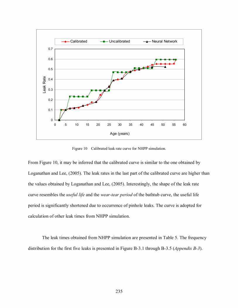
235
0
0.1
0.2
0.3
0.4
0.5
0.6
0.7
0 5 10 15 20 25 30 35 40 45 50 55 60
Age (years)
Leak
Rat
eCalibrated Uncalibrated Neural Network
Figure 10 Calibrated leak rate curve for NHPP simulation.
From Figure 10, it may be inferred that the calibrated curve is similar to the one obtained by
Loganathan and Lee, (2005). The leak rates in the last part of the calibrated curve are higher than
the values obtained by Loganathan and Lee, (2005). Interestingly, the shape of the leak rate
curve resembles the useful life and the wear-tear period of the bathtub curve, the useful life
period is significantly shortened due to occurrence of pinhole leaks. The curve is adopted for
calculation of other leak times from NHPP simulation.
The leak times obtained from NHPP simulation are presented in Table 5. The frequency
distribution for the first five leaks is presented in Figure B-3.1 through B-3.5 (Appendix B-3).

236
Table 5 Summary of results for various leak times from NHPP simulations.
Leak # Min. (year)
Max. (year)
Mean (year)
Mode (year)
Median (year)
Stand. Dev. (year)
Diff. in Mode
Diff. in Mean
1st Leak 2.019 31.051 9.488 3.793 7.862 6.067 2nd Leak 2.645 34.498 15.664 13.617 15.147 6.752 9.824 6.176 3rd Leak 3.618 42.630 20.197 24.328 20.860 6.504 10.711 4.533 4th Leak 5.845 44.888 23.659 26.260 23.935 6.082 1.932 3.462 5th Leak 8.475 44.985 26.622 33.830 26.314 5.884 7.570 2.963 6th Leak 8.833 46.799 29.313 36.243 29.014 5.802 2.412 2.691 7th Leak 13.962 50.650 31.719 38.702 31.406 6.002 2.459 2.406 8th Leak 16.926 54.418 33.885 41.056 33.323 6.014 2.354 2.165 9th Leak 18.059 59.010 36.089 43.611 35.322 6.196 2.556 2.205 10th Leak 19.816 62.470 38.084 44.912 37.430 6.241 1.301 1.995 11th Leak 20.561 63.765 40.107 46.601 39.466 6.324 1.689 2.022 12th Leak 23.944 65.000 41.960 49.759 41.379 6.529 3.158 1.853 13th Leak 24.133 66.905 43.730 50.272 43.277 6.569 0.512 1.770 14th Leak 26.891 67.749 45.604 50.329 45.107 6.702 0.058 1.875 15th Leak 29.284 69.802 47.411 51.067 46.913 6.876 0.737 1.806 16th Leak 30.774 75.835 49.160 52.466 48.840 7.079 1.399 1.749 17th Leak 33.980 76.690 51.010 52.905 50.692 7.105 0.439 1.850 18th Leak 34.852 78.822 52.802 53.695 52.656 7.329 0.790 1.792 19th Leak 35.565 80.412 54.474 57.018 54.160 7.562 3.323 1.671 20th Leak 36.149 83.437 56.307 57.806 56.042 7.596 0.788 1.833 21st Leak 39.076 83.560 58.106 59.965 57.959 7.823 2.159 1.799 22nd Leak 39.935 87.981 59.801 60.545 59.295 7.944 0.580 1.695 23rd Leak 39.949 88.374 61.462 62.090 60.762 8.132 1.545 1.661 24th Leak 40.027 93.641 63.262 62.576 62.338 8.333 0.485 1.800 25th Leak 40.532 95.935 64.824 62.637 63.973 8.520 0.061 1.562
The basis of the model building was to aid the decision process for replacement of the
plumbing system. The replacement criteria are discussed in the following section.
Replacement criteria
As discussed previously, the decision to replace the plumbing is subjective to one’s
choice. There may be several parameters that may govern the decision to opt for replacement.
Most of the time, cost considerations dominate the replacement criteria but there may be other
237
homeowners who may not like to consider the cost as a governing factor. This work presents the
replacement criteria based on cost. This criteria is based on the minimum cost, the optimal
replacement is determined so as to optimize the expenditure incurred by the homeowner
considering the useful life period of the plumbing system.
In order to arrive at the said criteria, first an assessment of the repair and replacement
cost is presented. The assessment of the cost is based on the Homeowner survey and the Plumber
Survey-II. Both these surveys were conducted by Virginia Tech Survey Research Center. The
surveys were conducted in 2005~2006 period, hence the cost data obtained from these surveys is
very valid for present.
Repair costs
From a homeowner’s perspective, the repair costs for the pinhole leak should not be
limited to the cost of repairing the leaks only. The cost should include the cost incurred in getting
the other damages repaired, cost of personal time spent, and cost of stress and any other cost
incurred in getting one’s life back to normal as it was before the leak. Unfortunately, such a data
is not only difficult to obtain but also it has a lot of variability associated with it, especially in the
cost of stress and cost of personal time. Hence, for estimation purposes the values that are
considered may be subjected to change under special circumstances. The following cost data is
based on 45 respondents from homeowner survey. These respondents had experienced pinhole
leaks in copper pipes in their homes. The cost data presented in the following section represents
the cost incurred by the respondents on all the leaks, the data does not provide costs incurred per
leak.

238
Amongst 45 respondents, 60 percent reported no other damage from the pinhole leak and
40 percent reported other damages (Figure 11). Thirty eight percent respondents paid less than $
100 for the repair of all the leak, about 29 percent paid between $ 101 ~ $ 500, fifteen percent
between $ 501 ~$ 1000, thirteen percent between $ 1001~ $ 3000 (Figure 12) . Hence, there is
considerable variability in the cost of repair.
0
0.1
0.2
0.3
0.4
0.5
0.6
0.7
Other damages-repaired No other damage Other damages- but notrepaired
Other damages due to pinhole leak
Rel
ativ
e Fr
eque
ncy
Figure 11 Analysis of damages due to pinhole leaks, based on 45 respondents from the survey.

239
0
0.05
0.1
0.15
0.2
0.25
0.3
0.35
0.4
< $100 $101~$500 $501~$1000 $1001~$3000 Don’t Know
Repair Cost for pinhole leak repair only
Rela
tive
Freq
uenc
y
Figure 12 Analysis of repair cost incurred to homeowners for repair of pinhole leaks.
About fifty percent of the homeowners found the experience very stressful or somewhat
stressful, twenty five percent found the experience not very stressful, while twenty percent did
not respond to the question (Figure 13).
0
0.05
0.1
0.15
0.2
0.25
0.3
0.35
Very Stressful Somew hatStressful
Not veryStressful
No response
Experience with pinhole leak
Rel
ativ
e Fr
eque
ncy
Figure 13 Analysis of stress experienced by homeowners in dealing with pinhole leaks.

240
Interestingly, majority of homeowners (50 percent) reported to have spent less than 10 hours
on the repairs, about 25 percent spent 11~ 20 hours, fifteen percent 21~ 40 hours, less than five
percent 41~ 80 hours and greater than 80 hrs respectively (Figure 14).
0
0.1
0.2
0.3
0.4
0.5
0.6
<10 hrs 11~20 hrs 21~40 hrs 41~80 hrs > 80 hrs
Personal time spent on pinhole leak
Rel
ativ
e Fr
eque
ncy
Figure 14 Analysis of personal time spent on repairs by homeowners in dealing with pinhole leaks.
Most of the homeowners could not provide any value for the total expenditure that was
incurred due to the leak incident. Hence, a comprehensive figure for the repair cost of the pinhole
leak cannot be obtained directly from the survey results. While majority of the homeowners
reported to have spent less than $ 100 as repair cost on all the leaks. The variability in the cost is
evident; the reason for the large variation in the cost may be due to small number of respondents
that have experienced leak.
Since, the data does not provide the repair cost data per leak, suitable assumption needs
to be made. If the cost of other damages, stress and personal time spent by the homeowner are

241
taken into account the total cost of repair including these can be assumed to be $ 500 per leak. A
repair cost of $ 500 per leak is used by Loganathan and Lee (2005).
Replacement cost
The modal value of the replacement cost or the cost of re-plumbing using copper pipes in
a two bedroom two bath, two-level home obtained from Plumber survey-II is $ 3000. Although,
there was a large variation in the cost of re-plumb but around 20 percent of the total 109
plumbers quoted the cost of re plumb between $ 2500 and $ 3000. Hence, the modal value of $
3000 (quoted by 12 plumbers) can be considered as a reasonable estimate. This estimate is in
agreement with the results of Plumber survey-I, where the quoted range was $ 2500 to $ 4000.
Hence, an estimate of $ 3000 for re-plumb is justifiable.
With the available estimates of repair and replacement cost, an optimal replacement
criteria is discussed. The other criteria based on the risk assessment, will be derived from the
threshold value of inter event time.
Cost Based Optimal Replacement
The cost based optimality is required to optimize the expenditures for repair or
replacement of the plumbing. Since, re-plumbing is about six times more expensive than
repairing it is not the best alternative to prevent a homeowner from pinhole leaks. However, after
certain leaks, the cost criteria may make the replacement viable from investment considerations.
Hence, an optimal criterion is required to determine the threshold stage at which the replacement
becomes viable.

242
Loganathan et al.(2002), derived the optimal replacement criterion based on the cost of
repairs, cost of replacement and the discount rate. The criterion is presented below,
( )RF
FF
C
tt n
n
n
n
nn +
+
<−
++
+ 1ln
ln 11
1 (9)
Where,
nn tt −+1 is the inter event time between the two successive failures.
1+nC is the cost of repair for the thn 1+ failure
nF is the cost of replacement at the time of the thn failure
1+nF is the cost of replacement at the time of the thn 1+ failure
The model was used by Loganathan and Lee, (2005), while determining the optimal
replacement. If it is assumed that the cost of repair and the cost of re-plumb do not change with
the failures, then it follows from above 3000$1 == +nn FF , 500$1 =+nC . Since, the cost of repair
and the cost of replacement is considered independent of inflation, the nominal discount rate
needs to be adjusted for inflation. A detailed discussion on the real rate, nominal rate and
inflation is presented in Appendix C-3. For nominal discount rate of 6 % and inflation rate of
3.39 % the real rate is 2.61 % (Appendix C-3)
From Eqn (9), we get

243
( )0261.01ln
13000500ln
1 +
+
<−+ nn tt ,
Or
yearstt nn 98.51 <−+ (10)
Hence, when the inter event time becomes less than 5.98 years, the option of replacement
become viable from cost considerations. This result can be used with the NHPP model to
determine the time of optimal replacement. From Table 5, if mean values for the leak times are
considered, then the inter event time between the second and the third leak is 4.533 years, hence
a replacement becomes viable at the second leak. The average age of the plumbing at the time of
third leak is 15.664 years (From Table 5). Hence, from replacement considerations, the second
leak or a fifteen year period after the installation, whichever is earlier should be used. The
criteria should be used only for the plumbing systems that have experienced at least one leak.
Conclusions
The analysis provides two different kinds of criteria that may help the homeowner in the
process of decision making. The leak rates are based on the CDA data and the homeowner
survey, hence, the results are applicable on a nationwide basis. Since, the exact synergy of the
causal factors that initiated the pinhole leaks are not understood, the model and the methodology
are very beneficial from a homeowner’s perspective.

244
The data and the criteria are applicable to the homes that have had at least one pinhole
leak, it should not be used to evaluate the homes where pinhole leaks have not been a problem.
In case, the plumbing system is replaced, the model should not be used for the new (replaced)
system till such time pinhole leaks incidents start in the new system.
References
1. Loganathan G.V and Lee J. (2005), Decision tool for optimal replacement of plumbing
systems, Civil Engineering and Environmental Systems 22, No. 4, 189-204.
2. Loganathan G.V., Park S. and Sherali H.D.,(2002), Threshold Break Rate for Pipeline
Replacement in Water Distribution Systems, Journal of Water Resources Planning and
Management, 128 (4), 271-279
3. Ross S.M. (2000), Introduction to Probability Models, edition 6th, Academic Press.
4. Sheikh A.K., Boah J.K., Hansen D.A.(1990), Statistical Modeling of Pitting Corrosion
and Pipeline Reliability, Corrosion Science, 46 (3), 190-197.
5. Gabrielli C., Huet F., Keddam M. and Oltra R.(1990), A Review of the Probabilistic
Aspects of Localized Corrosion, Corrosion Science, 46 (4), 266-278.
6. Rausand Marvin and Hoyland Arnljot (2004), System Reliability Theory, Models,
Statistical Models and Applications, edition 2nd , John Wiley and Sons Inc.
7. Rigdon Steven E. and Basu Asit P. (2000), Statistical Methods for the Reliability of
Repairable Systems, John Wiley and Sons Inc.
8. Copper Development Association (CDA), Failure reports 1975~2004.

245
9. Washington Suburban Sanitary Commission (WSSC), pinhole leak database.
10. Virginia Tech Survey Research Center, Homeowner Pinhole Leak and Drinking Water
Survey (2005).
11. Loganathan G.V., Lee Juneseok, Farooqi Owais, Plumber Survey-I (2005).
12. Virginia Tech Survey Research Center, Plumber Survey-II (2006).
Website References
13. http://www.wssc.dst.md.us
14. http://inflationdata.com
15. http://www.frbsf.org

Appendix A-3
246
APPENDIX A-3
Leak time Statistics and Distributions from CDA data base
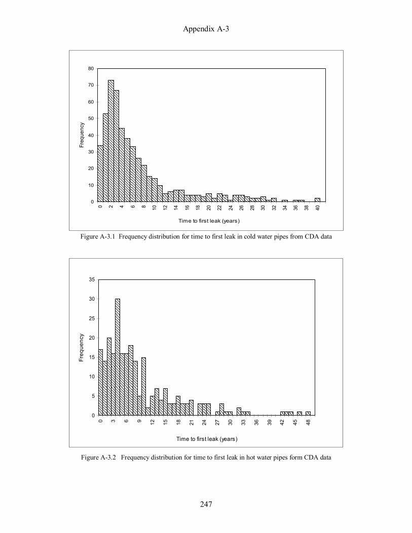
Appendix A-3
247
0
10
20
30
40
50
60
70
80
0 2 4 6 8 10 12 14 16 18 20 22 24 26 28 30 32 34 36 38 40
Time to first leak (years)
Freq
uenc
y
Figure A-3.1 Frequency distribution for time to first leak in cold water pipes from CDA data
0
5
10
15
20
25
30
35
0 3 6 9 12 15 18 21 24 27 30 33 36 39 42 45 48
Time to first leak (years)
Freq
uenc
y
Figure A-3.2 Frequency distribution for time to first leak in hot water pipes form CDA data

Appendix A-3
248
Table A-3.1 Descriptive Statistics for time to first leak in cold water pipes categorized by failure causes
Cause of failure Cou
nt
Min
imum
Max
imum
Mea
n
Med
ian
Mod
e
Stan
dard
E
rror
Stan
dard
D
evia
tion
Sam
ple
Var
ianc
e
Skew
nes
s
Ran
ge
Chloride/ Chlorine 236 0 37 6.26 4 3 0.410 6.29 39.64 2.146 37 Oxygen-differential 51 0 40 15.58 13 2 1.386 9.90 98.01 0.595 40 Failure initiated outside 67 0 40 4.87 3 0 0.838 6.86 47.06 3.329 40 Aggressive water 74 0 25 3.95 3 1 0.507 4.36 19.01 2.636 25 Erosion-Corrosion 43 0 32 6.60 4 1 1.098 7.20 51.86 1.760 32 Sulfide 16 1 34 9.25 8 8 1.762 7.04 49.67 3.135 33 Other minor 1 25 0 31 7.04 3 1 1.796 8.98 80.71 1.495 31Over All (average) 512 0 40 6.73 4 2 0.325 7.36 54.17 1.992 401 Minor Causes include poor workmanship, microbial, no cause ascertained or a combination of above reasons. All values reported are in years.
Table A-3.2 Descriptive Statistics for time to first leak in hot water pipes categorized by failure causes
Cause of failure Cou
nt
Min
imum
Max
imum
Mea
n
Med
ian
Mod
e
Stan
dard
E
rror
Stan
dard
D
evia
tion
Sam
ple
Var
ianc
e
Skew
nes
s
Ran
ge
Erosion-Corrosion 84 0 30 6.87 5.5 4 0.631 5.781 33.42 1.67 30 Excessive Heating of water 64 0 48 13.19 10 7 1.382 11.05 122.2 1.17 48 Failure initiated outside 40 0 43 6.85 4.5 4 1.234 7.804 60.9 3.01 43 Chloride/ Chlorine 24 0 29 7.5 5 4 1.556 7.621 58.09 1.72 29 Oxygen-differential 16 0 33 11.94 9 2 2.857 11.43 130.6 0.97 33 Other minor 2 23 0 46 9.96 7 7 2.19 10.52 110.8 1.99 46 Over All ( Average) 251 0 48 9.14 6 4 0.571 9.049 81.89 1.82 482 Minor Causes include poor workmanship, aggressive water, no cause ascertained or a combination of above reasons. All values reported are in years.
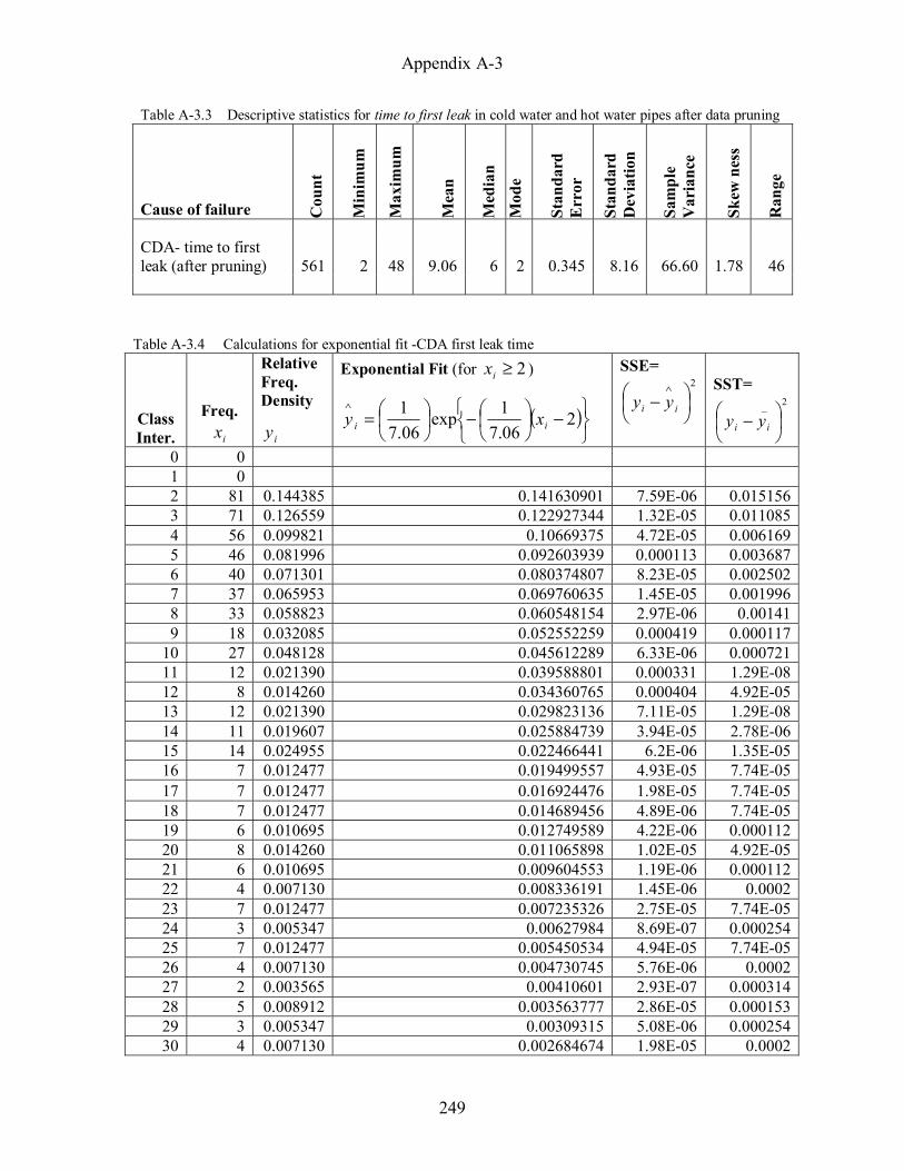
Appendix A-3
249
Table A-3.3 Descriptive statistics for time to first leak in cold water and hot water pipes after data pruning
Cause of failure Cou
nt
Min
imum
Max
imum
Mea
n
Med
ian
Mod
e
Stan
dard
E
rror
Stan
dard
D
evia
tion
Sam
ple
Var
ianc
e
Skew
nes
s
Ran
ge
CDA- time to first leak (after pruning) 561 2 48 9.06 6 2 0.345 8.16 66.60 1.78 46
Table A-3.4 Calculations for exponential fit -CDA first leak time
Class Inter.
Freq.ix
Relative Freq. Density
iy
Exponential Fit (for 2≥ix )
( )
−
−
=
∧2
06.71exp
06.71
ii xy
SSE= 2
−
∧
ii yy
SST=2_
− ii yy
0 0 1 0 2 81 0.144385 0.141630901 7.59E-06 0.0151563 71 0.126559 0.122927344 1.32E-05 0.0110854 56 0.099821 0.10669375 4.72E-05 0.0061695 46 0.081996 0.092603939 0.000113 0.0036876 40 0.071301 0.080374807 8.23E-05 0.0025027 37 0.065953 0.069760635 1.45E-05 0.0019968 33 0.058823 0.060548154 2.97E-06 0.001419 18 0.032085 0.052552259 0.000419 0.000117
10 27 0.048128 0.045612289 6.33E-06 0.00072111 12 0.021390 0.039588801 0.000331 1.29E-0812 8 0.014260 0.034360765 0.000404 4.92E-0513 12 0.021390 0.029823136 7.11E-05 1.29E-0814 11 0.019607 0.025884739 3.94E-05 2.78E-0615 14 0.024955 0.022466441 6.2E-06 1.35E-0516 7 0.012477 0.019499557 4.93E-05 7.74E-0517 7 0.012477 0.016924476 1.98E-05 7.74E-0518 7 0.012477 0.014689456 4.89E-06 7.74E-0519 6 0.010695 0.012749589 4.22E-06 0.00011220 8 0.014260 0.011065898 1.02E-05 4.92E-0521 6 0.010695 0.009604553 1.19E-06 0.00011222 4 0.007130 0.008336191 1.45E-06 0.000223 7 0.012477 0.007235326 2.75E-05 7.74E-0524 3 0.005347 0.00627984 8.69E-07 0.00025425 7 0.012477 0.005450534 4.94E-05 7.74E-0526 4 0.007130 0.004730745 5.76E-06 0.000227 2 0.003565 0.00410601 2.93E-07 0.00031428 5 0.008912 0.003563777 2.86E-05 0.00015329 3 0.005347 0.00309315 5.08E-06 0.00025430 4 0.007130 0.002684674 1.98E-05 0.0002

Appendix A-3
250
Table A-3.4 Calculations for exponential fit -CDA first leak time
Class Inter.
Freq.ix
Relative Freq. Density
iy
Exponential Fit (for 2≥ix )
( )
−
−
=
∧2
06.71exp
06.71
ii xy
SSE= 2
−
∧
ii yy
SST=2_
− ii yy
31 1 0.001782 0.00233014 3E-07 0.0003832 4 0.007130 0.002022425 2.61E-05 0.000233 1 0.001782 0.001755347 7.39E-10 0.0003834 2 0.003565 0.001523538 4.17E-06 0.00031435 0 0 0.001322342 1.75E-06 0.00045336 1 0.001782 0.001147716 4.03E-07 0.0003837 1 0.001782 0.00099615 6.18E-07 0.0003838 0 0 0.0008646 7.48E-07 0.00045339 0 0 0.000750422 5.63E-07 0.00045340 1 0.001782 0.000651323 1.28E-06 0.0003841 0 0 0.00056531 3.2E-07 0.00045342 1 0.001782 0.000490656 1.67E-06 0.0003843 0 0 0.000425861 1.81E-07 0.00045344 1 0.001782 0.000369622 2E-06 0.0003845 0 0 0.000320811 1.03E-07 0.00045346 1 0.001782 0.000278445 2.26E-06 0.0003847 0 0 0.000241674 5.84E-08 0.00045348 1 0.001782 0.000209759 2.47E-06 0.00038
=∑ ix 561
SSE= 0.001831
SST=0.052246
=_
iy 0.021276 =−=
SSTSSER 12 0.96496

Appendix B-3
251
APPENDIX B-3
Frequency distribution of leak times from Non-Homogenous Poisson
Process Simulations

Appendix B-3
252
0
10
20
30
40
50
60
70
80
0 2 4 6 8 10 12 14 16 18 20 22 24 26 28 30
Age (years)
Freq
uenc
y
Figure B-3.1 Frequency distribution for time to first leak from NHPP simulations.
.
0
5
10
15
20
25
30
35
40
0 2 4 6 8 10 12 14 16 18 20 22 24 26 28 30 32 34
Age (years)
Freq
uenc
y
Figure B-3.2 Frequency distribution for time to second leak from NHPP simulations.

Appendix B-3
253
0
5
10
15
20
25
30
35
40
45
50
0 2 4 6 8 10 12 14 16 18 20 22 24 26 28 30 32 34 36 38 40 42
Age (years)
Freq
uenc
y
Figure B-3.3 Frequency distribution for time to third leak from NHPP simulations.
0
10
20
30
40
50
60
0 2 4 6 8 10 12 14 16 18 20 22 24 26 28 30 32 34 36 38 40 42 44
Age (years)
Freq
uenc
y
Figure B-3.4 Frequency distribution for time to fourth leak from NHPP simulations.

Appendix B-3
254
0
10
20
30
40
50
60
0 2 4 6 8 10 12 14 16 18 20 22 24 26 28 30 32 34 36 38 40 42 44
Age (years)
Freq
uenc
y
Figure B-3.5 Frequency distribution for time to fifth leak from NHPP simulations.

Appendix C-3
255
APPENDIX C-3
Discussion on nominal and real interest rates

Appendix C-3
256
Interest Rate
The fee charged by the lender to the borrower is known as interest. It is generally
expressed as annual percentage of the principal amount. The principal amount is the amount
borrowed. For instance, if a person A borrows a sum of $ 100 from person B at an annual interest
rate of 10%, then the principal amount is $ 100 and at the end of one year period, person A needs
to pay $ 110 to person B to clear his debts. This method of calculation of interest is also known
as simple interest. In simple interest calculation, the interest is calculated only on the principal,
hence if the money is borrowed for 2 years, the amount that the person A needs to pay in order to
clear all the debts will be $ 120. No interest is charged on the amount accrued due to interest at
the end of the first year. The relationship between the simple interest and the principal amount is
given by,
100prtI = (C-1)
Where,
I is the interest in dollars
p is the principal amount in dollars
r is the rate of interest in annual percent
t is the time in years
Another method of calculating interest is the compound interest. In this method additional
interest is charged on the amount accrued due to interest at the end of every year. The total
amount payable by person A at compound interest is given by

Appendix C-3
257
nrpA
+=
1001 (C-2)
Where
A is the total amount to be paid by person A at the end of n years to clear all debts, in dollars
p is the principal amount in dollars
r is the rate of compound interest
Hence, if a person A borrows $ 100 from person B at a rate of 10% compound interest, then the
amount that the person A needs to pay at the end of one year in order to clear all his debts will be
From Eqn (C-2)
110100101100
1
=
+=A
Which is same as the amount to be paid by person A, had the money was borrowed on simple
interest. At the end of two year period, the amount to be paid by person A, will be
From Eqn (C-2)
121100101100
2
=
+=A
This is more than the amount that the person A would have paid, had he borrowed the money on
simple interest. The difference of $ 1 is due to added interest that is calculated on the interest
accrued at the end of the first year (i.e. $ 10).

Appendix C-3
258
Importantly, the rate of interest r does not account for inflation. Inflation is the measure of
increase in price of the goods or decrease in purchasing power of the currency with time, and is
expressed as annual percentage. Let us assume that the person A borrows $ 100 from person B
for a period of one year at 10% interest rate. For simplicity, let us assume a one year period as it
does not affect the method of calculation of interest (simple or compound). Hence, at the end of
one year period the person A returns $ 110 to person B to clear all his debts.
Apparently, the amount that the person B earned from the deal is $ 10 at the end of one
year, although during this 1 year period the prices of the good might have increased by some
percentage say 4% (assumed). Hence, the goods that were available at a price of $ 100 at the
time the money was lend are costing $ 104 at the time the money is returned, hence the net gain
to person B at the end of the deal should be $ 6 (= $10 - $ 4 or = interest – inflation). Thus, the
actual earning of person B from the deal is at 6% interest, if the inflation is accounted. By this
conclusion, we can define nominal and real interest rate. The nominal interest rate is the rate
stated on bond, it does not account for the inflation. The real interest rate is defined as the current
interest rate minus the current inflation rate. The nominal interest rate can be expressed in terms
of the real interest rate and the inflation, by Fisher equation, hence mathematically,
( ) ( )( )nrn irr ++=+ 111 (C-3)
Where
nr is the nominal rate of interest
rr is the real rate of interest
Appendix C-3
259
ni is the rate of inflation
By expanding Eqn (C-3) we get,
nrnrn irirr +++=+ 11
Or
nrnrn irirr ++= (C-4)
Since nrnr irir >+ , we can neglect nrir ,
Hence, Eqn (C-4) can be approximated by
nrn irr += (C-5)
The inflation rate varies depending upon the Consumer Price Index (CPI) and Producer Price
Index (PPI), these indices are generally calculated on a monthly basis. The averaged inflation
rate for the year 2005 is 3.39 %
http://inflationdata.com/Inflation/Inflation_Rate/HistoricalInflation.aspx
The current discount rate or the nominal rate is 6 %, based on Federal Reserve Bank of San
Francisco http://www.frbsf.org/banking/data/discount/index.html
Hence, using Eqn (C-5), the real rate will be
39.36 += rr
Appendix C-3
260
Or
=rr 2.61 %
Since, the cost of repair and cost of re-plumbing is assumed constant with time, real interest rate
should be used instead of the nominal rate.

261
CHAPTER-4
PINHOLE LEAKS- MECHANISTIC MODELLING
Corrosion Thermodynamics
Corrosion is the electrochemical degradation of a metal when exposed to the
environment. The phenomenon leading to corrosion is usually described using the laws of
thermodynamics and electrochemistry. The objective of most of the studies is to understand the
kinetics of the corrosion. Even during studying the kinetics, the rate of change must obey the
stoichiometric relationship. Much of the following description is based on Tretheway and
Chamberlain (1995). Most of the metals exist in impure (ore) state in nature. Thermodynamically
the natural state of any metal or element corresponds to its lowest energy state. The process of
extraction and refining of metals require a set of processes where substantial energy is
consumed. The energy consumed may vary in magnitude and form depending on the metal and
the extraction process itself.
This energy may be supplied to the process in the form of heat energy for blast furnaces,
electrical energy for electrochemical separation or any other form of energy such as nuclear
energy. A major part of the energy consumed in the purification process is stored in the metals in
the form of free energy. Hence the pure state of a metal corresponds to higher energy state, and
according to the laws of thermodynamics there exists an inherent tendency for substances at
higher energy state to transform to their lower energy states.

262
Thus pure metals are at higher energy states and are less stable, they are prone to
transformations to products that are at lower energy states and hence more stable. This tendency
of the metals is the driving force behind the corrosion phenomenon. The energy state of the
corrosion product is generally similar to the energy state of the metal ore, in some cases even
comparable. Figure 1, shows the relative difference in free energies of a metal and its lower
energy states on an arbitrary scale.
Corrosion Products
Pure Metal
Metal Ore
Activation Energy
CorrosionExtraction “Energy mounds”
Reaction Coordinates
Free
Ene
rgy
Figure 1 Schematic diagram showing Energy profile of metal and its corrosion products
The above definition of corrosion may altogether question the stability and hence the
existence of pure metals but in reality metals exists in pure form. The existence of metals in pure
state can be supported by the fact that there exists an energy barrier between any of the three
states (i.e. the metal ore, pure metal and the corrosion products).

263
Figure 1, shows the energy barrier in form of “energy mound”, which helps the metals to stay in
the pure states even though there is a strong tendency to corrode. Thus, for a metal in pure state
the energy barrier is the minimum activation energy that is needed to trigger a reaction, which
can take it to a lower energy state. According to the laws of thermodynamics, for the reaction to
occur spontaneously, the change in free energy for the reaction ( )reactionG∆ should be negative.
The change in free energy for a reaction is defined as the difference between the free energies of
the products and reactants. Mathematically, it can be written as
tsreacproductsreaction GGG tan∆−∆=∆ (1)
Figure 1, shows a negative free energy change for the corrosion process, hence corrosion
is a spontaneous process. Most of the metals exist in thermodynamically stable states, hence are
already corroded, this can be explained by the presence of a thin oxide film on the surface of the
metals, the presence of this film offers resistance to corrosion by protecting the metal from its
environment. The film is known as passivating film and the phenomenon is known as
passivation.
However, if the surface of metal is scratched with a sharp edged object, the film will get
damaged and the surface of the metal will be exposed to the environment. Upon exposure to
environment the damaged film can reinstate itself and hinder corrosion or it may get destroyed
and corrosion may propagate, the behavior of the passivating films in metals is extremely
complex and is very often dependent on the environmental conditions.
264
Corrosion and Electrochemistry
From electrochemical perspective, corrosion may be defined as a phenomenon where the
metal loses electrons (oxidized) to its environment. For conservation of charge, the environment
should accept the same number of electrons (reduced). The corrosion reactions are characterized
by the presence of two oppositely charged electrodes, the oxidation takes place at anode while
the reduction takes place at cathode. At anode the corroding metal loses electron and hence
moves to higher oxidation states, thermodynamically these oxidation states should correspond to
lower energy. It implies a direct correlation between the thermodynamics and the
electrochemical reaction involved in the corrosion phenomenon. The electrochemical behavior of
the corrosion reactions may be best described by using the electrochemical series. The concepts
to develop and arrive at electrochemical series are presented below.
Consider a rod of metal A dipped into an aqueous alkaline solution, since the metal has a
tendency to corrode, it will tend to lose electrons and move to higher oxidation state,
mathematically the reaction may be expressed as,
−+ +→ zeAA z
Where
z is the number of electrons involved in the reaction (also equal to the change in oxidation state
or is the number of electrons given up by the atom)

265
The metal ions tend to enter the electrolyte leaving behind a negatively charged metal
surface, thus by bringing the electrode to a negative potential. A setup of electrode and the
electrolyte put together is often named as a half cell and the reaction at the electrode is referred
as the half cell reaction. In order to overcome the difficulties associated with the measurement of
absolute value of the potential, hydrogen electrode is universally accepted as a reference
electrode. The electrode potential for hydrogen is arbitrarily accepted as zero at 298 K (25oC)
and 1 atmospheric pressure. Hence the electrode potentials for all the electrodes are expressed
either above (positive) or below (negative) of the hydrogen electrode under standard conditions.
These are also known as standard electrode potentials. As a conventional practice, the electrode
potentials may either be expressed for oxidation or reduction reactions. For example,
−+ +→ zeAA z BE +=0 Volts.
The above equation shows oxidation of metal A, hence the electrode potential when
measured under standard condition with reference to hydrogen electrode, will be known as
Standard Oxidation Potential. If the same equation is expressed as a reduction equation, then the
electrode potential when measured under standard condition with reference to the hydrogen
electrode is known as Standard Reduction Potential. The corresponding reduction equation may
be expressed as
AzeAz →+ −+ BE −=0 volts.
Both the conventions are equally acceptable, however the present work will follow the
Standard Reduction Potentials. The Standard Reduction Potentials are standard values, which are
constant for a metal under standard conditions; these values may be tabulated in a descending

266
order to obtain a series. The series is known as the electrochemical series and is considered as a
benchmark for all the corrosion reactions. The electrochemical series is presented below in Table
1.
Table 1 Electrochemical series Standard Reduction Potential (Source: http://en.wikipedia.org/wiki/Standard_electrode_potential_%28data_page%29 ).
Electrode reaction ( )VoltsE 0 AueAu =+ −+ +1.83
HgeHg =+ −+ 22 +0.85
AgeAg =+ −+ +0.80
sCueCu =+ −+ +0.52
CueCu =+ −+ 22 +0.34 +−+ =+ CueCu 2 +0.16
222 HeH =+ −+ 0.00
PbePb =+ −+ 22 -0.13
SneSn =+ −+ 22 -0.13
NieNi =+ −+ 22 -0.26
CdeCd =+ −+ 22 -0.40
FeeFe =+ −+ 22 -0.44
CreCr =+ −+ 33 -0.74
ZneZn =+ −+ 22 -0.76
AleAl =+ −+ 33 -1.68
MgeMg =+ −+ 22 -2.38
NaeNa =+ −+ -2.71
CaeCa =+ −+ 22 -2.76
KeK =+ −+ -2.93 The table is an abbreviated version of the table available on http://en.wikipedia.org. The information related to
copyright permission is available on http://en.wikipedia.org/wiki/Wikipedia:Copyrights.
An electrochemical cell necessarily consists of four elements, an anode, a cathode, an
electrolyte and a physical connection for passage of current. The Standard Reduction Potential
or the relative placement of a metal in the electrochemical series determines whether it will act as
an anode or as a cathode for that particular pair of electrodes. For example, let us consider iron
and zinc, since zinc is more noble to copper it shall act as anode, hence in a cell consisting of
267
zinc and iron electrodes, corrosion will occur at zinc while deposition will occur at iron. This is
the reason why zinc is used for galvanizing iron.
The total electrochemical cell potential is defined as the difference of cathodic and anodic
reduction potential, we may express cell potential as
000
anodecathodecell EEE −= (2)
Faradays related the change in free energy with the electrochemical cell potential by following
expression
( ) 00cellEzFG −=∆ (3)
Where
0G∆ is the change is free energy under standard conditions.
z is the number of electrons involved in the reaction (also equal to the change in oxidation state)
0cellE is the standard cell potential.
For reaction to be spontaneous the net change in free energy should be negative, it follows from
Eqn(3)
00 <∆G
Hence,

268
( ) 00 <− cellEzF
Or 00 >cellE (4)
Or 000 >− anodecathode EE (5)
The above inequality states that the electrode with lesser reduction potential in the
electrochemical series will act as anode for the reaction to be spontaneous. Since, the potential of
the half cell depends upon number of physical parameters like temperature, pressure,
concentration of electrolyte etc, and most of the reactions encountered in real life do not take
place under standard conditions, it is important to evaluate and arrive at an expression that can
take into account for all these parameters. Consider a reaction under non-standard conditions
++ +→+ zz YXYX
Using thermodynamics, the free energy change under non standard conditions, G∆ may be
expressed as
[ ][ ][ ][ ]+
+
+∆=∆ z
z
XYYXRTGG ln0 (6)
Where
G∆ is the change in free energy under non standard conditions
0G∆ is the change in free energy under standard conditions

269
R is the universal gas constant.
T is the absolute temperature in Kelvin
[ ]X & [ ]Y are the concentrations of solid X and Y respectively. (Generally taken as unity,
because it is assumed that the reaction is not limited by the concentration of these species)
[ ]+zX is the concentration of ion from metal X under non-equilibrium conditions.
[ ]+zY is the concentration of ion from metal Y under non-equilibrium conditions.
It follows from Faradays law stated above in Eqn(3),
( ) cellEzFG −=∆
and
( ) 00cellEzFG −=∆
Substituting the values for change in free energy in Eqn(6), we get
[ ][ ]+
+
+−=− z
z
YXRTzFEzFE ln0
Or
[ ][ ]+
+
−= z
z
YX
zFRTEE ln0 (7)
Eqn(7) is called the Nerst equation and has great theoretical and practical significance.

270
Corrosion Kinetics
Electrochemical reactions involve flow of electron from a negatively charged site (anode)
to a more positively charged site (cathode). As the current flow in the external circuit, the metal
ions flow from anode to cathode in the electrolyte. The flow of electrons can be measured as
electrical current, where 1 ampere is equal to 1 coulomb charge (6.2 x 10¹⁸ electrons) per second.
Faradays’ law relates the corrosion current and the mass reacted, by following expression
zFItam = (8)
Where
m is the mass transferred from anode in g
I is the current measured in coulombs per second
a is the molar mass of the metal in g per mol
z is the number of electrons participating in the reaction (also equal to the change in oxidation
state)
F is the Faraday’s constant in coulombs per mol-electrons
t is the time in seconds
Defining rate of reaction as r , then we may write
tAmr = (9)
271
Where
A is the surface area
Substituting the value of m from Eqn(9), we have
AzFIa
Itmr ==
Defining iAI = (current density) and substituting in the above expression we get,
zFiar = (10)
Since a , z and F are constants for a metal in a particular cell reaction, it follows that
ir ∝
The dimensional units of r in Eqn(10) are [ ]12 −− TML . The units may be converted to units
of penetration [ ]1−LT . The conversion of the units to r to mili-inches per year )(mpy reduces the
Eqn(10) to
zDair 129.0= (11)

272
Where,
r is the rate of corrosion measured in )(mpy
a is the molar mass of the metal g per mol
D is the density of the metal 3/ cmgm
i is the corrosion current density 2/ cmAµ
z is the number of electrons participating in the reaction (also equal to the change in oxidation
state)
Hence, the kinetics of the corrosion is solely dependent on the nature and variation of the
corrosion current density. The corrosion current density is defined as the difference between the
anodic and the cathodic current densities. Hence,
cameas iii −=
Where
ai is the anodic current density , and
ci is the cathodic current density.
iimeas = is the corrosion current density that is equal to the difference in anodic and cathodic
current densities.

273
At equilibrium the magnitude of the net corrosion current density becomes zero, although
there exists a current that flows in both the direction but it cannot be measured. This is called the
exchange current density and is denoted by 0i . Hence at equilibrium,
0iii ca ==
Due to surface defects, a metal can behave as its own anode and cathode when placed in
an electrolyte. Thus a single piece of metal may have anodic and cathodic sites that are
connected with the metal surface. When such a metal piece is dipped in an electrolyte it forms an
electrochemical cell. The anodic sites on the surface of the metal tend to lose electron, as the
current flows through the metal surface; there is a loss of positive metal ions at anode. Let us
analyze the process in terms of the corrosion current density and the change in free energy.
Consider a metal A placed in some electrolyte, Figure 2 shows the energy profile, at the
start of the reaction *G∆ is the energy barrier for the metal to undergo corrosion. Please note that
Figure 2 shows only the corrosion process from Figure 1, the other half that shows the metal
extraction is not shown. Initially the difference in the energy states of the metal and the corrosion
products is large. As the reaction proceeds the two states approach each other and hence *G∆
increases, while G∆ decreases. Thermodynamically, the rate of the anodic (forward) reaction
can be expressed in terms of the energy barrier *G∆ .
∆−=RTGra
*
expλ (12)

274
Where
*G∆ is the activation free energy for the forward reaction.
λ is a proportionality constant
R is the universal gas constant
T is the absolute temperature in Kelvin
Analysis of Eqn(12) suggests that as *G∆ increases the rate of the anodic reaction
decreases. Since the current density is directly proportional to the rate of the reaction, it would
imply that the anodic current density decreases as the reaction proceeds.
Corrosion Products
Pure Metal
Activation Energy = *G∆
Reaction Coordinates
Free
Ene
rgy
Difference in Free Energy = G∆
Figure 2 Schematic diagram showing activation energy of corrosion mechanism

275
Similarly the activation free energy for the backward reaction in the beginning of the
process is ( )GG ∆+∆ * , as the reaction proceeds G∆ decreases and *G∆ increases, and as both
the energy states of the metal becomes closer to each other the magnitude of ( )GG ∆+∆ *
decreases. Thermodynamically, the rate of cathodic reaction may be written as
( )
∆+∆−=RT
GGrc
*
expλ (13)
Where
( )GG ∆+∆ * is the activation free energy for the reverse reaction.
Since the rate of reaction is related to the current density, by analogy the rate of the
anodic and cathodic reactions should be related to anodic and cathodic current densities. It is
evident from Eqn(13) that the magnitude of ( )GG ∆+∆ * decreases as the reaction proceeds and
hence the magnitude of cathodic current density increases. Hence, during the initial stages of the
reaction ca ii > , as the reaction proceeds the magnitude of ai decreases and the magnitude of
ci increases, hence the corrosion current i decreases with the progress of the reaction.
Eventually a condition of thermodynamic equilibrium is achieved, under equilibrium
conditions, the activation free energies for forward and reverse reactions are equal; hence the
anodic and cathodic current densities will be equal. The magnitude of the anodic and cathodic
densities under such condition is equal to the exchange current density 0i . The values of 0i are
determined experimentally.
276
From the above analysis it is clear that the pure metal and the corrosion products
themselves do not remain in the same energy state, as the reaction proceeds the pure metal
moves into lower energy state while the corrosion products moves into higher energy state.
Hence the equilibrium between the metal and its corrosion product is disturbed, due to which the
electrode potential differs from the equilibrium potential, this difference is known as over
potential or the polarization ( )η . Polarization is a useful parameter in determining the kinetics of
the corrosion phenomenon. We further define α as the polarization proportionality, the
parameter α ranges between 0 and 1, it defines the extent of polarization of anode and cathode.
If the total polarization isη , then we can define ( )αη as the anodic polarization and ( )ηα−1 as
the cathodic polarization. At equilibrium the rate of the reaction and hence the exchange current
density may be expressed as
∆−=RTGi
*
00 expλ (14)
Where
0λ is a constant of proportionality and undetermined.
We can convert the anodic and cathodic overpotential into activation free energy using Faradays
law and hence
New activation energy for anodic reaction = ( )zFG αη−∆ *
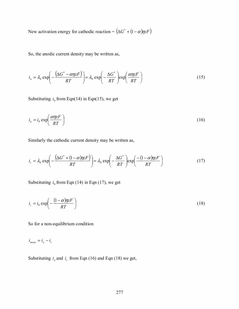
277
New activation energy for cathodic reaction = ( )( )zFG ηα−+∆ 1*
So, the anodic current density may be written as,
( )
∆−=
−∆−=RT
zFRTG
RTzFGia
αηλαηλ expexpexp*
0
*
0 (15)
Substituting 0i from Eqn(14) in Eqn(15), we get
=
RTzFiia
αηexp0 (16)
Similarly the cathodic current density may be written as,
( )( ) ( )
−−
∆−=
−+∆−=RT
zFRTG
RTzFGic
ηαληαλ 1expexp1exp*
0
*
0 (17)
Substituting 0i from Eqn (14) in Eqn (17), we get
( )
−−=
RTzFiic
ηα1exp0 (18)
So for a non-equilibrium condition
cameas iii −=
Substituting ai and ci from Eqn (16) and Eqn (18) we get,

278
( )
−−−
=
RTzF
RTzFiimeas
ηααη 1expexp0 (19)
Eqn (19) is known as Butler-Volmer Equation. This equation can be used to determine
the corrosion current and hence the rate of corrosion. The equation has two unknown parameters
η and 0i that needs to be determined experimentally. Both these parameters are specific function
of particular redox reaction and are dependent on many physical parameters such as
concentration of electrolyte, temperature, ratio of the oxidized and reduced species which makes
it impossible to determine them theoretically. However, if these two parameters are available
then Eqn (16) may be considered as a strong approach for calculating the corrosion rates.
Corrosion kinetics: Linear Polarization Approach
In order to arrive at an expression that is useful from analytical perspective, a simplified
approach is presented. The approach is based on the correlation between polarization and the
corrosion current density. In the previous section it was demonstrated that the activation free
energies change with the progress of the corrosion reaction. The anodic and the cathodic current
densities also change as the activation free energy changes. Since the rate of anodic and cathodic
current densities are related to the anodic and cathodic polarization (refer Eqn (15 & Eqn (17)),
the polarization should also vary with the corrosion current density. A plot of polarization vs the
current density, is known as polarization curve. Figure, 3 shows a typical polarization curve. For
small magnitudes current density, the polarization curve is almost linear (shown in dotted
rectangle).

279
Anodic Current Density
Cathodic Current Density
Ano
dic
pola
rizat
ion
Cat
hodi
c po
lariz
atio
n
Linear part of polarization curve
Figure 3 Typical polarization curve, showing linear zone between polarization and current density
In order to arrive at a simplified expression for calculating the current density, it is
assumed that the corrosion takes place in the linear part of the polarization curve. Hence, a new
parameter polarization resistance pR is defined as the slope of the polarization curve in this
region. We may write,
did
iRp
ηη =∆∆= (20)
The quantity didη can be obtained from Butler-Volmer equation (Eqn (19)).
We have,

280
( )
−−−
=
RTzF
RTzFiimeas
ηααη 1expexp0 (Butler-Volmer Equation)
Differentiating Eqn (19) with respect toη , we get
( ) ( )
−−
−−−
=
RTzFi
RTzF
RTzFi
RTzF
ddimeas ηαααηα
η1exp1exp 00 (21)
From Eqn (16) and Eqn (18), we have,
=
RTzFiia
αηexp0
( )
−−=
RTzFiic
ηα1exp0
By reverse substitution of ai and ci , in Eqn (21) we get
( )
−−−
= ca
meas iRT
zFiRTzF
ddi αα
η1 (22)
Let us define two more parameters, aβ and cβ as the anodic and cathodic Tafel coefficients. We
define,
zFRT
a αβ 303.2= (23)

281
( )zFRT
c αβ
−=
1303.2 (24)
Substituting the values of pR , aβ and cβ in Eqn (22) we get,
c
c
a
a
p
iiR ββ
303.2303.21 += (25)
For linear behavior of Tafel equation at both anode and cathode, the anodic and the
cathodic current densities should be approximately equal to the corrosion current density
(independently).
Hence,
measa ii ~ (26)
And
measc ii ~ (27)
Substituting measi from Eqn (26) & Eqn (27) in Eqn (25) we get,
( )cap
ca
cap
meascorr RR
iiββ
ββ
ββ+
=
+
==303.211303.2
1 (28)

282
Or
pcorr R
Ki = , where ( )ca
caKββ
ββ+
=303.2
Eqn (28) is known as the Linear Polarization equation, notice that the Tafel constants
aβ and cβ are fixed parameters for a reaction at a particular temperature, hence, the corrosion
current becomes the function of one variable pR .
Examples
Example1
A single family residential home is located in an area that is prone to pinhole leaks.
Knowing that pinhole leak is inevitable, the homeowner wants to know when he should expect
the first leak in his house. The homeowner knows that the pipes used in his plumbing system are
( )"2/1 & ( )"4/3 nominal diameter, M-type copper.
With this information he approaches a consultant, who is doing research on the pinhole leaks in
single family homes; the consultant has some historical data collected from a nationwide survey.
However, due to busy schedule, the consultant could not offer his services to the homeowner, but
as a gesture of goodwill he handed over some valuable information that can be used to calculate
the time to first leak. The information given by the consultant is presented in the Table 2.
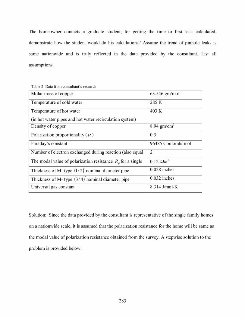
283
The homeowner contacts a graduate student, for getting the time to first leak calculated,
demonstrate how the student would do his calculations? Assume the trend of pinhole leaks is
same nationwide and is truly reflected in the data provided by the consultant. List all
assumptions.
Table 2 Data from consultant’s research
Molar mass of copper 63.546 gm/mol
Temperature of cold water 285 K
Temperature of hot water
(in hot water pipes and hot water recirculation system)
403 K
Density of copper 8.94 gm/cm3
Polarization proportionality (α ) 0.3
Faraday’s constant 96485 Coulomb/ mol
Number of electron exchanged during reaction (also equal 2
The modal value of polarization resistance pR for a single 0.12 2mΩ
Thickness of M- type ( )"2/1 nominal diameter pipe 0.028 inches
Thickness of M- type ( )"4/3 nominal diameter pipe 0.032 inches
Universal gas constant 8.314 J/mol-K
Solution: Since the data provided by the consultant is representative of the single family homes
on a nationwide scale, it is assumed that the polarization resistance for the home will be same as
the modal value of polarization resistance obtained from the survey. A stepwise solution to the
problem is provided below:

284
Step 1: Calculating the Tafel coefficients from given data
The anodic and the cathodic Tafel coefficients aβ and cβ are given by,
( )zF
RTa α
β 303.2= (E1-1)
And
( )( )zF
RTc α
β−
=1303.2 (E1-2)
Where,
R = universal gas constant in J/mol-k
α = polarization proportionality
T = absolute temperature in Kelvin
z = number of electron participation or the change in oxidation state.
F = Faradays’ constant in Coulomb/ mol
From the consultant’s data we have,
R = 8.314 J/mol-k
α = 0.3
T = 285 K (cold water)
T = 403 K (hot water)
z = 2
F = 96485 Coulomb/ mol

285
For cold water pipes
Substituting the values in Eqn (E1-1) & Eqn (E1-2), we get
( )( )( )( )( ) 094262.0
9648523.0285314.8303.2 ==aβ
And
( )( )( )( )( ) 040398.0
9648523.01285314.8303.2 =
−=cβ
For hot water pipes
Substituting the values in Eqn (E1-1) & Eqn (E1-2), we get
( )( )( )( )( ) 13329.0
9648523.0403314.8303.2 ==aβ
And
( )( )( )( )( ) 057124.0
9648523.01403314.8303.2 =
−=cβ
Step 2: Calculating the corrosion current density using Linear polarization equation
The linear polarization equation relates the corrosion current density and the polarization
resistance by following expression:
( )( ) )(303.2 cap
ca
Ri
ββββ
+= (E1-3)
Where,
i is the corrosion current density in 2/ mA

286
aβ is the anodic Tafel coefficient
cβ is the cathodic Tafel coefficient
pR is the polarization resistance in 2m−Ω
For cold water pipes
We have,
094262.0=aβ (from Step-1)
040398.0=cβ (from Step-1) and
212.0 mRp Ω= (from consultants’ data)
Substituting aβ , cβ and pR in Eqn (E1-3), we get
( )( )( ) ( ) ( )( )
2/10232.0040398.0094262.012.0303.2
040398.0094262.0 mAi =+
=
For hot water pipes
We have,
13329.0=aβ (from Step-1)
057124.0=cβ (from Step-1) and
212.0 mRp Ω= (from consultants’ data)
Substituting aβ , cβ and pR in Eqn (E1-3), we get
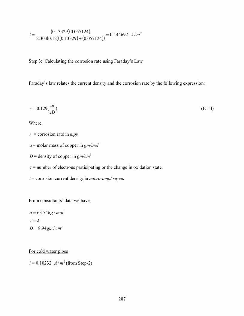
287
( )( )( ) ( ) ( )( )
2/144692.0057124.013329.012.0303.2
057124.013329.0 mAi =+
=
Step 3: Calculating the corrosion rate using Faraday’s Law
Faraday’s law relates the current density and the corrosion rate by the following expression:
)(129.0zDair = (E1-4)
Where,
r = corrosion rate in mpy
a = molar mass of copper in gm/mol
D = density of copper in gm/cm3
z = number of electrons participating or the change in oxidation state.
i = corrosion current density in micro-amp/ sq-cm
From consultants’ data we have,
3/94.82
/546.63
cmgmDz
molga
==
=
For cold water pipes
2/10232.0 mAi = (from Step-2)

288
For hot water pipes
2/144692.0 mAi = (from Step-2)
Converting i in 2/ cmAµ
For cold water pipes
224
62 /232.10/
101010232.0/10232.0 cmAcmAmAi µµ =
==
For hot water pipes
224
62 /469.14/
1010144692.0/144692.0 cmAcmAmAi µµ =
==
Substituting a , i , D and z in Eqn (E1-4), we get
For cold water pipes
( ) ( )( )( )( ) mpyr 691.4
94.82232.10546.63129.0 ==
For hot water pipes
( ) ( )( )( )( ) mpyr 6336.6
94.82469.14546.63129.0 ==
Step 4: Calculating the time to first leak from the corrosion rate
Assuming the rate of corrosion is same for both the pipe sizes. The rate may be expressed
as the thickness of incision through the pipe wall, divided by the time. If t is the pipe wall

289
thickness in inches and T is the time to first leak in years, and r be the rate of corrosion in mili-
inches per year (mpy), then
Ttr 1000= (E1-5)
Solving for T, we have
rtT 1000= (E1-6)
The rate in Eqn (E1-6) is equal to the one calculated in Step-3, hence the time to first leak will
depend on the thickness of the pipe. For thick walled pipes, the time to first leak will be more as
compared to thin walled pipes.
We define
1t as the thickness (in inches) of ( )"2/1 nominal diameter
2t as the thickness of (in inches) ( )"4/3 nominal diameter
1T as the time to first leak (in years) for ( )"2/1 nominal diameter
2T as the time to first leak (in years) for ( )"4/3 nominal diameter
Then from Eqn (E1-6) we have,
rt
T 11
1000= (E1-7)
And

290
rt
T 22
1000= (E1-8)
We have
1t = 0.028 inches (from consultant’s data)
2t = 0.032 inches (from consultant’s data)
For cold water pipes
mpyr 691.4=
Substituting 1t and r in Eqn (E1-7) we have,
( )( ) .968.5
691.4028.01000
1 yearsT ==
Similarly, substituting 2t and r in Eqn (E1-8) we have,
( )( ) .821.6
691.4032.01000
2 yearsT ==
For hot water pipes
mpyr 6336.6=
Substituting 1t and r in Eqn (E1-7) we have,
( )( ) .220.4
6336.6028.01000
1 yearsT ==
Similarly, substituting 2t and r in Eqn (E1-8) we have,
( )( ) .824.4
6336.6032.01000
2 yearsT ==

291
Hence, in cold water pipes, the first leak in ( )"2/1 pipe will occur after 5.97 years and the first
leak in ( )"4/3 inch pipe will occur after 6.82 years. For hot water pipes, the first leak in ( )"2/1
pipe will occur after 4.22 years and the first leak in ( )"4/3 inch pipe will occur after 4.824 years.
The results from the above approach suggest that an increase in temperature increases the
corrosion rate however this is highly subjective to water chemistry. As discussed previously in
chapter 2, the effect of temperature can be deleterious specially if the water has low alkalinity
and low DIC (dissolved inorganic carbon).
Example 2
You are a corrosion scientist and you live in a community that is developing very fast.
Unfortunately, the community had several incidences of pinhole leaks in the recent past. A real
estate builder, who has got major contracts for building new homes, is interested in knowing the
time to first leak for M-type copper pipes, so that he may give an option of other plumbing
materials to his new clients. He has set up a laboratory to run experiments and obtain information
that may be utilized to calculate the time to first leak. The builder has accumulated some data
which is shown in Table 3.
The builder approaches you with a set of parameters and requests your services as a consultant.
He also requests you to show all the calculations and assumptions as a part of the consultancy
report. Calculate the time to first leak for ( )"2/1 and ( )"4/3 nominal diameter pipes and show
what calculations you shall be putting in your report?

292
Table 3 Corrosion data provided by the builder Temperature of water 285 K
Polarization proportionality (α ) 0.3
Faraday’s constant 96485 Coulomb/ mol
Over- potential ( )η 0.16 Volts
Exchange current density ( )0i for Cu electrode in 0.1 N
HCL solution (Fontana, 1986)
0.2 2/ cmAµ
Thickness of M- type ( )"2/1 nominal diameter pipe 0.028 inches
Thickness of M- type ( )"4/3 nominal diameter pipe 0.032 inches
Universal gas constant 8.314 J/mol-K
Molar mass of copper 63.546 gm/mol
Density of copper 8.94 gm/cm3
Solution: Since the builder has provided the values for exchange current density ( )0i and the
over- potential ( )η , we may use the Butler-Volmer equation for calculating the corrosion current
density. Once the corrosion current density is obtained, Faradays’ law can be used to get the
corrosion rate. A step wise approach is presented below:
Step-1: Calculating corrosion current density from Butler-Volmer Equation
The Butler-Volmer equation may be written as
=measi ( )
−−−
RTzF
RTzFi ηααη 1expexp0 (E2-1)
Where
measi is the corrosion current density
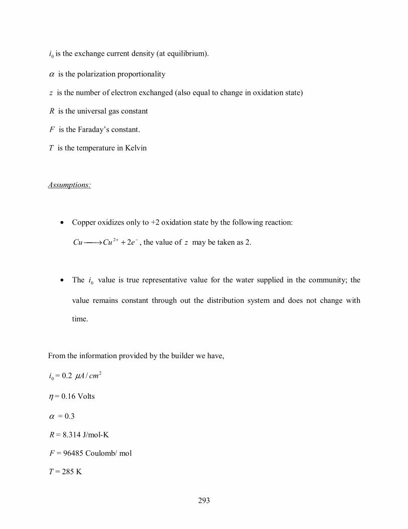
293
0i is the exchange current density (at equilibrium).
α is the polarization proportionality
z is the number of electron exchanged (also equal to change in oxidation state)
R is the universal gas constant
F is the Faraday’s constant.
T is the temperature in Kelvin
Assumptions:
• Copper oxidizes only to +2 oxidation state by the following reaction:
−+ +→ eCuCu 22 , the value of z may be taken as 2.
• The 0i value is true representative value for the water supplied in the community; the
value remains constant through out the distribution system and does not change with
time.
From the information provided by the builder we have,
0i = 0.2 2/ cmAµ
η = 0.16 Volts
α = 0.3
R = 8.314 J/mol-K
F = 96485 Coulomb/ mol
T = 285 K

294
z =2 (from our assumption)
Substituting in Eqn (E2-1) we get,
=measi ( ) ( )( )( )( )( )( )
( )( )( )( )( )( )
−−−
285314.8
96485216.03.01exp285314.8
96485216.03.0exp2.0
( ) == sayiimeas 9.9707 2/ cmAµ
Step-2: Calculating corrosion rate using Faraday’s Law
Faraday’s law relates the current density and the corrosion rate by the following expression:
)(129.0zDair = (E2-2)
Where,
r = corrosion rate in mpy
a = molar mass of copper in gm/mol
D = density of copper in gm/cm3
z = number of electrons participating or the change in oxidation state.
i = corrosion current density in micro-amp/ sq-cm
From the builders’ data we have,

295
3/94.8/546.63cmgmDmolga
==
And
2/9707.9 cmAi µ= (from Step-1)
z =2 (from our assumption)
Substituting the values in Eqn (E2-2), we get,
( ) ( )( )( )( ) mpyr 571.4
94.829707.9546.63129.0 ==
Step 3: Calculating the time to first leak from the corrosion rate
Assuming the rate of corrosion is same for both the pipe sizes. The rate may be expressed as the
thickness of incision through the pipe wall, divided by the time. If t is the pipe wall thickness in
inches and T is the time to first leak in years, and r be the rate of corrosion in mili-inches per
year (mpy), then
Ttr 1000= (E2-3)
Solving for T, we have
rtT 1000= (E2-4)

296
The rate in Eqn (E2-4) is equal to the one calculated in Step-2, hence the time to first leak will
depend on the thickness of the pipe. For thick walled pipes, the time to first leak will be more as
compared to thin walled pipes.
We define
1t as the thickness (in inches) of ( )"2/1 nominal diameter
2t as the thickness of (in inches) ( )"4/3 nominal diameter
1T as the time to first leak (in years) for ( )"2/1 nominal diameter
2T as the time to first leak (in years) for ( )"4/3 nominal diameter
Then from Eqn (E2-4) we have,
rt
T 11
1000= (E2-5)
And
rt
T 22
1000= (E2-6)
We have
1t = 0.028 inches (from consultant’s data)
2t = 0.032 inches (from consultant’s data)
mpyr 571.4= (from Step-2)

297
Substituting 1t and r in Eqn (E2-5) we have,
( )( ) .125.6
571.4028.01000
1 yearsT ==
Similarly, substituting 2t and r in Eqn (E2-6) we have,
( )( ) .00.7
571.4032.01000
2 yearsT ==
Hence, the first leak in ( )"2/1 pipe will occur after 6.125 years and the first leak in ( )"4/3 inch
pipe will occur after 7.0 years.
Further discussion on linear polarization
The equation has been used by various scientists to evaluate corrosion rates of different
metals. Zhang et al. (2002) used the linear polarization approach to study the instantaneous
corrosion rates of naturally patinated copper during continuous rain using the electrochemical
impedance spectroscopy. Abhijit and Pehkonen (2000) used the linear polarization approach to
assess the performance of corrosion scales in corrosion inhibition in copper pipes in water
distribution system. Hiromoto et al. (2000) used the approach in studying the effect of pH on the
polarization behavior of 5.17105.765 CuNiAlZr , as amorphous alloy due to presence of chloride ion.
The strength of the polarization approach is that the corrosion rates can be obtained by
knowing just a single parameter ( pR ). Hence, if the distribution of pR is known with age of the
plumbing, the corrosion rates and time to failures can be obtained using Eqn (28) and Eqn (11).
In all of the above cited works, the laboratory setups were used to establish the pR values. Hence,

298
the linear polarization approach though reduces the number of variables as compared to Butler-
Volmer equation, but it needs some experimental support to establish the pattern of pR with
variation of age of the metal and water chemistry.
The following section demonstrates a possible method of analysis based on linear
polarization method. The pitting phenomenon necessarily involves two steps, the pit initiation
and the pit propagation. The initiation of the pit may be immediate upon exposure or may be
delayed (Melchers, (2005)). Also, the rate of propagation of the pits vary, some of the pits
propagate faster and cause early failure, some pits propagate at a slower rate and cause a
relatively delayed failure, while some other pits stop propagating after certain time, the
phenomenon is often known as meta- stable pitting (Melchers,(2005)). The meta- stable pits may
reactivate after some time and propagate to cause failure. Thus the exact modeling of pit growth
based on corrosion current is fairly complex and it requires experimental data under different
hydraulic and water quality conditions. From modeling perspective, the variation of corrosion
current with age of the plumbing is of interest. Considering the complexity in calculation of
corrosion rates due to varied initiation and propagation, the corrosion current distribution based
on only the first leak time is presented. The distribution is obtained using the time to first failure
distribution from chapter-3.
If the time to first failure is known, then the corrosion rate equation can be used to obtain
corrosion current using Eqn (11), for a given pipe thickness. Once the corrosion current is
known, the polarization resistance ( pR ) can be calculated in terms of corrosion current and the

299
Tafel slopes. Hence, if the pipe of thickness 1t (inches) is considered that developed the first leak
after jT years of installation, then the rate of corrosion can be expressed as
jTtr 11000= mili-inches per year (29)
From Eqn (11) we have,
zDai
r 129.0=
Where,
r is the rate of corrosion for the first leak, measured in )(mpy
a is the molar mass of the metal gm per mol
D is the density of the metal 3/ cmgm
i is the corrosion current density 2/ cmAµ
z is the number of electrons participating in the reaction (also equal to the change in oxidation
state)
By substituting the value of r in Eqn (29) we get,
jTt
zDai 11000129.0 =

300
Or
)129.0())(1000( 1
aTzDti
j
= (30)
Eqn (30) provides the corrosion current in terms of pipe thickness; age of plumbing, molar mass
of copper, density of copper and the number of electrons lost by copper during the corrosion
reaction. The corrosion current can be used to obtain the polarization resistance pR , using Eqn
(28),
From Eqn (28) we have
pcorr R
Kii == , where ( )ca
caKββ
ββ+
=303.2
However, the units of i in Eqn (28) are 2/ mA , hence by changing the units of i to 2/ cmAµ
using the conversion, 1 2/ cmAµ = 22 /10 mA− and substituting i in Eqn (30) we get,
)129.0())(1000)(10( 1
2
aTzDt
RK
jp
−
=
Or
))(10()129.0(
1 zDtaKT
R jp =
546.63=a gm/ mol (the molar mass of copper)

301
94.8=D 3/ cmgm (density of copper)
2=z (number of electrons lost, as copper changes from 0 to +2 oxidation state)
Hence,
1
)(0459.0
tTK
R jp = (31)
where ( )ca
caKββ
ββ+
=303.2
zFRT
a αβ 303.2=
( )zFRT
c αβ
−=
1303.2
Hence, ifα , T and 1t is assumed, then using the distribution for first leak time (chapter 3), the
distribution for pR can be calculated.
For a M-type ½- inch copper pipe, the thickness 028.01 =t inches,
for 3.0=α
285=T K,
314.8=R J/mol-K
F = Faraday’s constant= 96485 Coulomb/ mol
1T = 3.79 years, modal time to first leak from chapter-3, we have

302
)96485)(2)(3.0()285)(314.8(303.2=aβ = 0.0942
( )( )( )( )( ) 040398.0
9648523.01285314.8303.2 =
−=cβ
K = 0.01227
From Eqn (31),
076.0028.0
)79.3)(01227.0(0459.0 ==pR 2mΩ
The distribution of corrosion current and polarization resistance for the first leak is shown in
Figure 4 and 5.

303
0
5
10
15
20
25
30
35
0 5 10 15 20 25 30 35
Time to f irst leak (years)
Cor
rosi
on C
urre
nt (M
icro
Am
p/ S
q-cm
)
Figure 4 Distribution of corrosion current with age of the plumbing for first leak.
0
0.1
0.2
0.3
0.4
0.5
0.6
0.7
0 5 10 15 20 25 30 35
Time to first leak (years)
Pol
ariz
atio
n R
esis
tanc
e (O
hm-S
qm)
Figure 5 Distribution of polarization resistance with age of the plumbing for first leak.

304
The distributions in Figure 4 and 5 are based on the first leak time distribution from
chapter-3. The corrosion rate decreases hyperbolically with age for the first leak distribution; the
corresponding polarization resistance shows a linear increase with age. Due to complexities
associated with delayed initiation and meta-stable pitting, the other leak times cannot be used
directly to obtain similar distributions of corrosion rate with age. For simulating conditions
similar to home plumbing systems, the variation of corrosion current and the polarization
resistance with age is needed for different hydraulic and water quality conditions. This needs
experimental support and can be useful for further research.
Conclusions
The two approaches namely Butler-Volmer equation and linear polarization approach
can be used for mechanistic modeling of copper corrosion. Both the approaches require
experimental data based on anion chemistry, pH and temperature for obtaining parameters that
are needed to model copper corrosion. The linear polarization approach requires lesser
parameters than the Butler-Volmer equations, however, the former is derived based on certain
assumptions and hence the results from the former would be less accurate.
From modeling perspective, the distribution of corrosion parameters with age of the
plumbing is needed. The distribution of polarization resistance and corrosion current is
presented based on first leak distribution; however the distribution of other leak times could not
be used directly due to complexities associated with delayed initiation and meta-stable pitting.
The approach needs experimental support for obtaining distribution of corrosion current with
age, under different hydraulic and water quality conditions.
305
References
1. Corrosion for science and engineering, Kenneth R. Trethewey, John Chamberlain, 2nd
edition, Longman, (1995), Chapter 4- The theory of aqueous corrosion, 69-129.
2. Corrosion Engineering Fontana, 3rd edition, McGraw Hill, 1986.
3. Zhang X., He W.,Wallinder I.O., Pan J., Leygraf C.(2002), Determination of
Instantaneous corrosion rates and runoff rates of copper from naturally patinated copper
during continuous rain events, Corrosion Science 44, 2131-2151.
4. Sun E.X., Nowak W.B.(2001), Electrochemical characteristics of Ti-6Al-4V alloy in 0.2
N NaCl solution I. Tafel slopes in quassi-passive state, Corrosion Science, 43, 1801-
1816.
5. Palit A., Pehkonen S.O.(2000), Copper corrosion in distribution systems: evaluation of a
homogenous Cu2O film and a natural corrosion scale as corrosion inhibitors, Corrosion
Science 42, 1801-1822.
6. Hiromoto S., Tsai A.-P., Sumita M.,Hanawa T.(2000), Effect of chloride ion on the
anodic polarization behavior of the 5.17105.765 CuNiAlZr amorphous alloy in phosphate
buffered solution, Corrosion Science 42, 1651-1660.
7. Hiromoto S., Tsai A.-P., Sumita M.,Hanawa T.(2000), Effect of pH on the polarization
behavior of 5.17105.765 CuNiAlZr amorphous alloy in a phosphate buffered solution,
Corrosion Science 42, 2193-2200.
8. El-Feki A.A., Walter G.W. (2000), Corrosion rate measurements under condtions of
mixed charge transfer plus diffusion control including the cathodic metal ion deposition
partial reaction, Corrosion Science, 42, 1055-1070.
306
9. Melchers R.E. (2005), Statistical Characterization of Pitting Corrosion- Part 1: Data
Analysis, Corrosion Science 61 (7), 655- 664.
10. Melchers R.E. (2005), Statistical Characterization of Pitting Corrosion- Part 1:
Probabilistic Modeling for Maximum Pit Depth, Corrosion Science 61 (8), 766- 777.
Website References
11. http://en.wikipedia.org

307
OWAIS E. FAROOQI
Owais was born on June 4th, 1975 in India. It was his interest in mechanics that led him to
University of Roorkee (now IIT-Roorkee) to pursue Engineering. He completed his Bachelors
degree in Civil Engineering in 1998 and joined Maruti-Suzuki as an engineering trainee. His
career in Maruti-Suzuki was marked by achievements and accolades. He designed and
implemented rainwater harvesting system in Maruti-Suzuki, the project was a pioneering effort
by the organization towards the arrest of the depleting ground water table. The success of the
project and his noble motives to serve the human kind brought him to United States to pursue
Masters Degree in Civil Engineering (Water Resources). His interests include studying and
designing BMPs, optimizing BMPs and forecasting. After completing his degree he will move to
Maryland to join a leading consulting firm in water industry. He intends to start a non-profit
organization at a later part of his career. He firmly believes in “think big- achieve big”
philosophy. He is a big fan of English and Urdu poetry.