AN ARCHITECTURAL DIMENSIONS BASED

SOFTWARE FUNCTIONAL SIZE MEASUREMENT METHOD

A THESIS SUBMITTED TO

THE GRADUATE SCHOOL OF INFORMATICS

OF

THE MIDDLE EAST TECHNICAL UNIVERSITY

BY

ÇİĞDEM GENCEL

IN PARTIAL FULFILLMENT OF THE REQUIREMENTS FOR THE DEGREE OF

DOCTOR OF PHILOSOPHY

IN

THE DEPARTMENT OF INFORMATION SYSTEMS

JULY 2005

PLAGIARISM

I hereby declare that all information in this document has been obtained and

presented in accordance with academic rules and ethical conduct. I also

declare that, as required by these rules and conduct, I have fully cited and

referenced all material and results that are not original to this work.

Name, Surname: Çiğdem Gencel Signature: _________________

Approval of the Graduate School of Informatics _________________________ Assoc.Prof.Dr. Nazife BAYKAL

Director

I certify that this thesis satisfies all the requirements as a thesis for the degree of Doctor of Philosophy. __________________________ Assoc.Prof.Dr. Onur DEMİRÖRS

Head of Department

This is to certify that we have read this thesis and that in our opinion it is fully adequate, in scope and quality, as a thesis for the degree of Doctor of Philosophy. _________________________ Assoc.Prof.Dr. Onur DEMİRÖRS

Supervisor

Examining Committee Members Prof.Dr. Semih BİLGEN (METU, EEE) __________________________

Assoc.Prof.Dr. Onur DEMİRÖRS (METU, IS) __________________________

Assoc.Prof.Dr. Ali DOĞRU (METU, CENG) __________________________

Assist.Prof.Dr. Kayhan İMRE (HU, CENG) __________________________

Dr. Altan KOÇYİĞİT (METU, IS) __________________________

iv

ABSTRACT

AN ARCHITECTURAL DIMENSIONS BASED SOFTWARE FUNCTIONAL SIZE MEASUREMENT METHOD

Gencel, Çiğdem

Ph.D., Department of Information Systems

Supervisor: Assoc.Prof.Dr. Onur Demirörs

July 2005, 300 pages

This thesis study aims to examine the conceptual and theoretical differences of Functional

Size Measurement (FSM) methods, to identify the improvement opportunities of these

methods and to develop a new FSM method. A comprehensive literature review is

performed and two multiple-case studies are conducted as a research strategy. In the light

of the results obtained, some improvement suggestions on two of the most challenging

improvement opportunities identified for FSM methods are made – improvement

opportunities which are related to the conceptual and theoretical basis of FSM and the

extension of the applicability of these methods to different software functional domain

types. The work behind these suggestions involves the critical examination of the concepts

“functionality” and “functional size” and the depiction of “types of functionality”

considering the components of software architecture and the forms of information

processing logic performed in different software functional domain types. Based on the

suggestions made, a new FSM method, called ARCHItectural DIMensions Based FSM (ARCHI-

DIM) is developed conforming to the ISO/IEC 14143-1 standard. A third multiple-case study

is conducted in order to evaluate the new method and to identify future directions for FSM

methods.

Keywords: Software size measurement, Functional size measurement, Functionality

v

ÖZ

MİMARİ BOYUTLARA DAYANAN YENİ BİR YAZILIM FONKSİYONEL BÜYÜKLÜK ÖLÇME YÖNTEMİ

Gencel, Çiğdem

Doktora, Bilişim Sistemleri Bölümü

Tez Yöneticisi: Doç.Dr. Onur Demirörs

Temmuz 2005, 300 sayfa

Bu çalışma Fonksiyonel Büyüklük Ölçme (FBÖ) yöntemlerinin kavramsal ve kuramsal

farkılıklarını araştırmayı, bu yöntemler için iyileştirme fırsatlarını belirlemeyi ve yeni bir

FBÖ yöntemi geliştirmeyi amaçlamaktadır. Kapsamlı bir literatür taraması yapılmış ve

araştırma stratejisi olarak iki çok-örnekli olay incelemesi yürütülmüştür. Bulgular ışığında,

FBÖ için belirlenmiş iyileştirme fırsatlarından önemli iki iyileştirme fırsatı olan FBÖ

yöntemlerinin kavramsal ve teorik bazlarının iyileştirilmesi ve uygulanabilirliklerinin farklı

yazılım fonksiyonel alan türleri için genişletilmesi ile ilgili öneriler getirilmiştir. Bu

önerilerin arkasında yatan çalışma; “fonksiyonellik” ve “fonksiyonel büyüklük”

kavramlarının eleştirel olarak incelenmesini ve yazılım mimari ögeleri ile farklı yazılım

fonksiyonel alan tiplerindeki bilgi işleme mantığı biçimlerini dikkate alarak “fonksiyonellik

tipleri” nin belirlenmesini içermektedir. Getirilen öneriler baz alınarak ISO/IEC 14143-1

standardına uyumlu Mimari Boyutlara Dayanan FBÖ (ARCHI-DIM) olarak adlandırılmış yeni

bir yöntem geliştirilmiştir. Bu yöntemi değerlendirmek ve gelecek araştırma doğrultularını

belirlemek için üçüncü bir çoklu-örnek olay incelemesi yürütülmüştür.

Anahtar kelimeler: Yazılım büyüklük ölçme, Fonkiyonel büyüklük ölçme, Fonksiyonellik

vi

DEDICATION

To Hatice, Kemal and Özgür Gencel

vii

ACKNOWLEDGMENTS

I express my sincere appreciation to my supervisor Onur Demirörs, not only for

accepting me to study with him, but also for his guidance, his stimulating suggestions and

insightful comments throughout my research. I am grateful to him for his friendship, his

faith in me and for letting me to study in a friendly and relaxing atmosphere.

I also want to thank my committee members Semih Bilgen, Altan Koçyiğit, Ali

Doğru and Kayhan İmre for their valuable suggestions and comments. I am grateful to Altan

Koçyiğit also for his physical and moral support, which helped me a lot during my hard

times. His support, at a very critical time during my PhD study, is invaluable.

The technical assistance, close collaboration and moral support of Erhan Yüceer is

gratefully acknowledged. His friendship is one of the most valuable gains of this research. I

also want to thank his wife Ahu and their little son Can for their infinite patience.

I want to express my appreciation to Oktay Türetken for the valuable discussions

we made on this thesis study during the coffee breaks. His contribution to this research is

significant.

Thanks go to Pınar Efe for her close collaboration and for providing me the data in

conducting the case study part of this research.

I wish to express my gratitude to Neşe Yalabık who continuously supported me

throughout my PhD study.

Many thanks to Ayça Tarhan, Onur Su, Meltem Sönmez and Burcu Akkan for their

valuable suggestions and moral support.

I want to thank Nil Korkut for her assistance in reviewing and proofreading some of

the work related to this research and for offering me valuable suggestions.

viii

Special thanks to Cihan Yıldırım, Seçil Canbaz Hüseyinoğlu, Umut Hüseyinoğlu and

Yasemin Salihoğlu. Their continous support and encouragement have been a source of

strength. I will never forget the special gift of Umut Hüseyinoğlu - a poem of Cavafy -

which he thought that resembles my road of PhD.

Heartfelt thanks to Cüneyt Sevgi for his continual encouragement, his tireless

assistance, helpful suggestions and critical comments. I am deeply indebted to him for his

enthusiasm for what I do and his endless physical and moral support through all the stages

of my PhD study.

Finally, I would like to thank my family - my brother, my mom and my dad - for

being there for me whenever I needed them, and for their love, understanding, patience,

and unshakable faith in me. They are my inspiration to find the power in my heart for

doing what I want in my life*.

My thanks and apologies to others whom I may have inadvertently forgotton to

mention.

* Son olarak aileme – kardeşime, anneme ve babama - ihtiyaç duyduğum her zaman yanımda oldukları için ve sevgileri, anlayışları, sabırları ve bana olan sarsılmaz güvenleri için teşekkür etmek istiyorum. Onlar benim hayatta istediğim her şeyi yapabilmem için kalbimdeki gücü bulmamda ilham kaynaklarım.

ix

Ithaca When you set out on your journey to Ithaca, pray that the road is long, full of adventure, full of knowledge. The Lestrygonians and the Cyclops, the angry Poseidon -- do not fear them: You will never find such as these on your path, if your thoughts remain lofty, if a fine emotion touches your spirit and your body. The Lestrygonians and the Cyclops, the fierce Poseidon you will never encounter, if you do not carry them within your soul, if your soul does not set them up before you. Pray that the road is long. That the summer mornings are many, when, with such pleasure, with such joy you will enter ports seen for the first time; stop at Phoenician markets, and purchase fine merchandise, mother-of-pearl and coral, amber and ebony, and sensual perfumes of all kinds, as many sensual perfumes as you can; visit many Egyptian cities, to learn and learn from scholars. Always keep Ithaca in your mind. To arrive there is your ultimate goal. But do not hurry the voyage at all. It is better to let it last for many years; and to anchor at the island when you are old, rich with all you have gained on the way, not expecting that Ithaca will offer you riches. Ithaca has given you the beautiful voyage. Without her you would have never set out on the road. She has nothing more to give you. And if you find her poor, Ithaca has not deceived you. Wise as you have become, with so much experience, you must already have understood what Ithacas mean. Constantine P. Cavafy (1911)

x

TABLE OF CONTENTS

PLAGIARISM .............................................................................................. ii

ABSTRACT............................................................................................... iv

ÖZ......................................................................................................... v

DEDICATION............................................................................................. vi

ACKNOWLEDGMENTS ................................................................................. vii

TABLE OF CONTENTS ................................................................................... x

LIST OF TABLES ....................................................................................... xii

LIST OF FIGURES .......................................................................................xv

LIST OF ACRONYMS / ABBREVIATIONS ............................................................. xvi

CHAPTER ................................................................................................. 1

1 INTRODUCTION .................................................................................... 1 1.1 Scope of the Thesis Study ............................................................. 3 1.2 Research Strategy ...................................................................... 3 1.3 Road Map ................................................................................ 4

2 RELATED RESEARCH............................................................................... 6 2.1 Software Size Metrics .................................................................. 6 2.2 Software Size Estimation / Measurement Methods ................................ 8

2.2.1 Derived Measurement / Estimation Methods .................................... 9 2.2.2 Classification of Software Size Measurement Methods........................22

2.3 The Differences between FSM Methods ............................................27 2.4 Discussion of the Literature Survey Results........................................36

xi

3 A NEW FSM METHOD: ARCHI-DIM FSM..........................................................40 3.1 Overview................................................................................40 3.2 The Need for a New Approach for Counting Software Functional Size.........41 3.3 ARCHI-DIM FSM Method and the Measurement Guidelines .......................48

3.3.1 Introduction .........................................................................48 3.3.2 ARCHI-DIM Measurement Process - The Method and the Rules ..............52

4 CASE STUDIES ON FUNCTIONAL SIZE MEASUREMENT.........................................65 4.1 Research Methodology ................................................................65 4.2 Case Studies on the Implementation of FSM Methods ............................69

4.2.1 Case Study 1: Utilizing Size Estimation Methods Early in the Life Cycle ...70 4.2.2 Case Study 2: Implementation of FSM Methods to Different Application

Domains .......................................................................................84 4.2.3 Case Study 3: Implementation of ARCHI-DIM FSM ........................... 107

5 CONCLUSIONS ................................................................................... 131 5.1 Contributions to the Field of Software Engineering ............................ 132

5.1.1 Improvement Opportunities of FSM Methods ................................. 132 5.1.2 Development of a New FSM Method: ARCHI-DIM FSM........................ 149

5.2 Suggestions for Future Research .................................................. 151

6 BIBLIOGRAPHY .................................................................................. 153

APPENDICES........................................................................................... 159

A .................................................................................................... 160

B .................................................................................................... 164

C .................................................................................................... 177

VITA.................................................................................................... 300

xii

LIST OF TABLES

Table 1 Software Size Measurement Methods Based on “Functionality” Metric ..............12 Table 2 Parts of ISO/IEC 14143: Information Technology - Software Measurement -

Functional Size ..................................................................................13 Table 3 Criteria for the Classification of Software Size Measurement Methods ..............22 Table 4 BFC Types of Methods Based on “Functionality” Metrics...............................25 Table 5 Main Differences between IFPUG FPA, Mk II FPA and COSMIC FFP Methods .........32 Table 6 Forms of Processing Logic Performed by BFC Types of FSM Methods.................44 Table 7 Characteristics by Field of Application ...................................................46 Table 8 Forms of Processing Logic and Software Functionality Types .........................47 Table 9 The Naming Convention used in Case Study 2 and Case Study 3 ......................70 Table 10 Size Estimates of the Subsystems of the Case Project by Mk II FPA.................74 Table 11 Size Estimation of Module A1 by COSMIC FFP...........................................76 Table 12 Size Estimation of Module A1 by IFPUG FPA ............................................76 Table 13 Taxonomy for Defining Software Projects ..............................................77 Table 14 Elements of the EFPA Method ............................................................78 Table 15 EFPA Size Estimates for Consecutive Stages............................................79 Table 16 Size Estimates by EFPA at Consecutive Stages and the Relative Errors with respect

to Mk II FPA Estimate ...........................................................................81 Table 17 Efforts Utilized for the Life Cycle Processes of Project-1 ............................87 Table 18 Case Study 2.1 Mk II FPA Size Measurement Details ...................................88 Table 19 Case Study 2.1 COSMIC FFP Size Measurement Details................................88 Table 20 The Productivity Rates (Code & Unit Test Effort / Functional Size) of the

Subsystems of Case Study 2.1 .................................................................89 Table 21 The Productivity Rates (Development Effort/Functional Size) of Case Study2.1..89 Table 22 The Productivity Rates (Code & Unit Test Effort / SLOC) of Case Study 2.1.......89 Table 23 The Productivity (Development Effort / SLOC) Values of Case Study 2.1 ..........90 Table 24 The Ratio of Functional Size (Mk II FP & Cfsu) to SLOC Values of Case Study2.1..90 Table 25 Efforts Utilized for the Life Cycle Processes of Case Study 2.2......................92 Table 26 Case Study 2.2 Mk II FPA Size Measurement Details ...................................93 Table 27 Case Study 2.2 COSMIC FFP Size Measurement Details ................................93

xiii

Table 28 The Productivity Rates (Code & Unit Test Effort/Funct. Size) of Case Study 2.2 .94 Table 29 The Productivity Rates (Development Effort/Functional Size) of Case Study2.2..94 Table 30 The Productivity (Code & Unit Test Effort / SLOC) Values of Case Study 2.2 .....94 Table 31 The Productivity (Development Effort / SLOC) Values of Case Study 2.2 ..........95 Table 32 The Ratio of Functional Size (Mk II FP & Cfsu) to SLOC Values of Case Study2.2..95 Table 33 Efforts Utilized for the Life Cycle Processes of Case Study 2.3......................96 Table 34 Case Study 2.3 Mk II FPA Size Measurement Details ...................................97 Table 35 Case Study 2.3 COSMIC FFP Size Measurement Details ................................98 Table 36 The Productivity (Code & Unit Test Effort / Functional Size) Rates of Project-3.98 Table 37 The Productivity (Effort / Functional Size) Values of Case Study 2.3...............98 Table 38 SLOC Values of Case Study 2.3 ...........................................................99 Table 39 Case Study-2 Mk II FPA Size Measurement Details ................................... 100 Table 40 Case Study-2 COSMIC FFP Size Measurement Details ................................ 101 Table 41 The Efforts Utilized for Functional Size Measurement in Case Study 2 ........... 107 Table 42 Case Study 3.1 ARCHI-DIM FSM Size Measurement Details .......................... 109 Table 43 SLOC Values of Project-1 ................................................................ 111 Table 44 Case Study 3.2 ARCHI-DIM FSM Size Measurement Details .......................... 113 Table 45 SLOC Values of Project-3 ................................................................ 114 Table 46 The Code and Unit Test Effort Values of Project-3.................................. 114 Table 47 Case Study 3.3 ARCHI-DIM FSM Size Measurement Details .......................... 115 Table 48 The Productivity (Code & Unit Test Effort / Functional Size) Rates of Project-3116 Table 49 Mapping BFC Types of Mk II FPA and COSMIC FFP to the Constituent Parts of

ARCHI-DIM FSM BFCs .......................................................................... 118 Table 50 Summary of the Base Counts obtained by Mk II FPA, COSMIC FFP and ARCHI-DIM

FSM .............................................................................................. 119 Table 51 The Functional Sizes (Mk II FP, Cfsu and ADfsu) and SLOC Values of the

Subsystems of Project-1...................................................................... 122 Table 52 The Ratios of the Functional Sizes and SLOC Values of the Subsystems of Project-1

................................................................................................... 123 Table 53 The Ratio of SLOC to Functional Size of the Subsystems of Project-1 ............ 124 Table 54 The Functional Sizes of the Subsystems of Project-1 Obtained by Mk II FPA,

COSMIC FFP with respect to ARCHI-DIM FSM Dimensions ................................ 125 Table 55 The Ratios of SLOC to Functional Size (Mk II FP and Cfsu) of the Subsystems of

Project-1 ....................................................................................... 126

xiv

Table 56 Efforts Utilized for Functional Size Measurement by MkII FPA, COSMIC FFP and

ARCHI-DIM FSM................................................................................. 129 Table 57 The Correlation between Functional Size and Effort................................ 143 Table 58 The Ratio of SLOC to Functional Size (Cfsu) .......................................... 144 Table 59 The Ratio of SLOC (SmallTalk) to Functional Size (IFPUG FP)...................... 145 Table 60 The Ratio of SLOC (C++) to Functional Size (IFPUG FP) ............................. 146 Table 61 The Ratio of SLOC (Cobol) to Functional Size (IFPUG FP)........................... 147 Table 62 The Ratio of SLOC (C) to Functional Size (IFPUG FP)................................ 148

xv

LIST OF FIGURES

Figure 1 FSM Process of IFPUG FPA, Mk II FPA and COSMIC FFP.................................29 Figure 2. ARCHI-DIM Measurement Process ........................................................50 Figure 3. ARCHI-DIM Software Model................................................................57 Figure 4 Case Study Method..........................................................................68 Figure 5 Requirements Analysis Life Cycle.........................................................72

xvi

LIST OF ACRONYMS / ABBREVIATIONS 3-D : Three-Dimensional ADfsu : ARCHI-DIM FSM functional size unit ARCHI-DIM FSM : Architectural Dimensions Based FSM Method ASSET- R : Analytical Software Size Estimation Technique – Real-Time BFC : Base Functional Component BPM : Business Process Modeling CAS : Collision Avoidance Subsystem Cfsu : Cosmic Functional Size Unit CLOC : Commented Lines of Code COCOMO : Constructive Cost Model COP : Component Object Points COSMIC : Common Software Measurement International Consortium COTS : Commercial Off-The Shelf DET : Data Element Type DF : Data Function DFD : Data Flow Diagram DSI : Delivered Source Instructions E : Entry E&Q : Early and Quick eEPC : Extended Event Driven Process Chain EFP : Early Function Points EFPA : Early Function Point Analysis EI : External Input EIF : External Interface File EO : External Output EP : Elementary Process EQ : External Inquiry E-R : Entity - Relationship ES : Executable Statements F : Functions FBÖ : Fonksiyonel Büyüklük Ölçme FFP : Full Function Points FiSMA : The Finnish Software Metrics Association fP : Functional Primitive FP : Function Point FPA : Function Point Analysis FSM : Functional Size Measurement FUR : Functional User Requirement GL : Granularity Level GUI : Graphical User Interface HTML : Hyper Text Markup Language I : Input ICASE : Integrated Computer Aided Software Engineering IDEF : Integrated Computer Aided Manufacturing (I-CAM) Definition IFPUG : International Function Point Users Group IIU : Instance Interaction Unit

xvii

ILF : Internal Logical File ISBSG : International Software Benchmarking Standards Group ISO : International Standards Organization LD : Logical Data Group LOC : Lines of Code LT : Logical Transaction m : meter MDIU : Master Detail Interaction Unit MF : Macrofunction mF : Microfunction MIS : Management Information System MK II FPA : Mark II Function Point Analysis NCLOC : Non-Commented Lines of Code NEFPUG : The Netherlands Function Point Users Group NESMA : The Netherlands Software Metrics Users Association NOC : Average Number of Children per Base Class O : Output OO : Object Oriented OOmFP : Object Oriented Method Function Points OOFP : Object Oriented Function Points OP : Object Points PE : Processing Entity PIU : Population Interaction Unit POPs : Predictive Object Points R : Read RA : Resolution Advisory RET : Record Element Type RFP : Request for Proposal SELAM : Software Engineering Laboratory in Applied Metrics SGML : Standard Generalized Markup Language SLOC : Source Lines of Code SOM : Statistical Object Model SPR : Software Productivity Research SRS : Software Requirements Specification SSM : Software Sizing Model Std.Dev. : Standard Deviation SW-CMM : Software Capability Maturity Model TCAS : Traffic Collision Avoidance Subsystem TF : Transactional Function UAW : Unadjusted Actor Weight UKSMA : United Kingdom Software Metrics Association UML : Unified Modeling Language UUCP : Unadjusted Use Case Points UUCW : Unadjusted Use Case Weights VAF : Value Adjustment Factor W : Write X : Exit XML : Extensible Markup Language

1

CHAPTER

CHAPTER I

1 INTRODUCTION

Software Engineering requires measuring the attributes of software to be able to

describe, prescribe, and predict. Tom De Marco states, “If you can’t measure it, you can’t

manage it”. That is, we need to estimate how much software to build, just as we need to

determine the weight and volume of an engineering product as part of the planning

process.

Estimation errors are essential cause of poor management which usually results in

runaway projects that spiral out of control (Glass, 2002). Whatever these projects produce

is frequently behind schedule and over budget, and most often they fail to produce any

product at all. According to the Standish Group CHAOS report of 2003:

- 5% of software projects are terminated before they produce anything,

- 66% are considered to have failed,

- Of those that do complete the average cost blowout is 43%,

- The lost dollar value for USA projects in 2002 is estimated at US$38 billion with

another US$17 billion in cost overruns.

The question of what causes runaway projects arises frequently in the software

engineering field. One of the major causes of runaway projects is considered to be

immature measurement / estimation.

All prior software effort and cost estimation research is based on the supposition

that size is a primary predictor. One of the significant challenges of software engineering

remains to be reliable sizing of software. By estimating software size, it is possible to

estimate development effort, which enables to estimate cost. Therefore, the primary

metric that must be identified is the one that infers size attribute.

2

Various approaches to software size estimation are developed and applied in

different phases of the development life cycle during the last 3 decades. The size of

software can be estimated by classifying different types of externally observable features,

and then by counting the occurrences of those features. Examples for these features may

be inputs and outputs from a software component. Each estimation method counts

different types of features in a different way. There might also be differences in the

methods due to different application domains (MIS, real-time, control, etc.) which have

different features that should be considered.

Among the various size estimation methods, the ones based on “functionality” are

widely-used due to their earlier applicability during the software life cycle. After the

description of the original method based on “functionality to be delivered to the users” by

Albrecht (1979), variations of these methods have been developed. During the 1980s and

1990s, several authors have suggested new Function Point counting techniques that

intended to improve the original Function Point Analysis (FPA) or extend its field of

application from business application software to real-time and algorithmic software

(Symons, 2001).

In 1996, the International Standards Organization (ISO) started a working group

(ISO/IEC JTC1 SC7 WG12) to establish common principles of the methods based on

“functionality”. They first published the first part of this standard (ISO/IEC 14143-1,

1998), which defines the fundamental concepts of Functional Size Measurement (FSM) such

as “Functional Size”, “Base Functional Components (BFC)”, “BFC Types”, the FSM method

characteristics and requirements that should be met by a candidate method to be

conformant to this standard. The standard promoted the consistent interpretation of FSM

principles. After that, IEEE Std. 14143.1 (2000), which is an adoption of ISO/IEC 14143-

1:1998, was published.

Four more parts of ISO/IEC 14143, which are ISO/IEC 14143-2 (2002) - Conformity

evaluation of software size measurement methods to ISO/IEC 14143-1:1998; ISO/IEC TR

14143-3 (2003) - Verification of FSM methods; ISO/IEC TR 14143-4 (2002) - FSM Reference

model and ISO/IEC TR 14143-5 (2004) - Determination of functional domains for use with

FSM, were published in the following years.

Being conformant to ISO/IEC 14143-1 (1998), detailed descriptions of four FSM

methods which are IFPUG Function Point Analysis (ISO/IEC 20926, 2003), Mark II Function

Point Analysis (ISO/IEC 20968, 2002), COSMIC Full Function Points (ISO/IEC 19761, 2003)

3

and NESMA Function Point Analysis (ISO/IEC 24570, 2003) have been recently published as

ISO standards.

Although it has gone a long way, FSM is still considered as “immature” and

criticized because of the general difficulty of the measurement process and the

immaturity of the measurement science for software engineering (Hughes, 2000; Fenton,

1994; Fenton, 1996). The results of the literature review showed that there still exist

significant improvement opportunities for the existing FSM methods related to their

conceptual and theoretical basis, convertibility of functional sizes obtained by different

methods, estimation early in the life cycle, suitability of methods for different application

domains, and validation and rigor which are available in other engineering disciplines.

1.1 Scope of the Thesis Study

This thesis study aims to explore the improvement opportunities of FSM methods

and based on the findings, suggest some improvements and develop a new FSM method by

making improvements on two of the most challenging improvement opportunities, which

are on the conceptual and theoretical basis of FSM and extension of the application

domain suitability.

The research objectives of this thesis study are:

- to examine the conceptual and theoretical differences between FSM methods,

- to explore the applicability of FSM methods to measure the size of the projects

of different functional domain types,

- to explore the applicability of size estimation methods at different phases of

the software development life cycle,

- to bring into light the improvement opportunities related to FSM methods,

- to make some improvement suggestions and

- to develop a new FSM method based on the improvement suggestions.

1.2 Research Strategy

In order to assist to meet the research objectives of this thesis study, we

performed empirical studies on FSM methods. There are several ways of doing empirical

research in software engineering, which may include formal experiments, surveys and case

4

studies. We used case study as a research strategy in this thesis study, as we have no

control over behavioral events and we are examining contemporary events.

Three case studies are conducted as part of this thesis study. The first case study

is a single-case study which was conducted to explore the applicability of four estimation

methods at different phases of the software development life cycle.

The second case study is a multiple-case study which involves three different

cases. In this multiple case study, our objective is to explore the applicability of FSM

methods to measure the size of the projects of different functional domain types, examine

the differences between these methods and by evaluating the methods bring into light the

improvement opportunities related to FSM methods.

The third case study is also a multiple-case study. In this case-study our aim is to

explore the applicability of the new FSM method we introduced in Chapter 3: ARCHI-DIM

FSM. We applied ARCHI-DIM FSM to the same applications as in the second case study in

order to evaluate the improvement suggestions that motivate us to design this new

method.

1.3 Road Map

In Chapter II, the results of the literature review on software size metrics and

measurement / estimation methods are presented. The classification criteria we defined

for software size measurement methods are given. At the end of this chapter, the

differences between the conceptual and theoretical basis of FSM methods are analyzed

and discussed considering the concepts defined in ISO/IEC 14143-1 (1998) standard on FSM.

In Chapter III, in the light of the results we obtained by reviewing the literature

and conducting case studies, we make some improvement suggestions on the conceptual

and theoretical basis of FSM and application domain applicability. The work behind this

approach involve critical examination of the concepts “functionality” and “functional

size”, depicting “types of functionality” regarding the components of software

architecture and forms of processing logic. At the end of this chapter, we introduce a new

FSM method, called ARCHItectural DIMensions Based FSM (ARCHI-DIM).

In Chapter IV, the three multiple-case studies we conducted in this thesis study are

discussed.

5

In Chapter V, the lessons which are drawn from this research are presented. The

contributions of this research to the field of software engineering - the improvement

opportunities identified by making inferences with the case study results and development

of a new FSM method - and other suggestions for future work are discussed in this chapter.

6

CHAPTER II

2 RELATED RESEARCH

This chapter presents the results of the literature review on software size

measurement / estimation methods and metrics.

2.1 Software Size Metrics

With the new development methodologies, understanding of software product size

has become a concept which is related to other attributes such as; the length of the code,

functionality delivered to the users, amount of reuse and complexity of the development

(Fenton, 1996; Poel, 1998). Accordingly, software size measurement process has involved a

wide range of metrics and methods from the traditional to the new ones.

Length Metrics. The metrics to measure “code length” are easiest to measure. They can be

expressed in terms of Lines of Code (LOC), number of characters and so on. LOC is the

oldest and most widely used traditional size metric which is the key input to most software

cost/effort, productivity and quality measurements. It has also been used for

normalization of other metrics (Fenton, 1996). Although the oldest one, it is still the most

popular size metric since it is objective, easy to understand and measure. However, since

LOC is language-dependent, programs written in different languages cannot be directly

compared. Accurate measurement of LOC is possible only at the later stages of a project

when the code is written. Measurement in the early phases of a project when no code is

available can only be done by expert measurement.

LOC has been used in various ways (Fenton, 1996). Sometimes the blank lines and

comments are not counted while counting LOC; called “Non-commented Lines of Code

(NCLOC)”. In other cases, not only NCLOC but also the “Comment Lines of Code (CLOC)”

are counted. The total size is calculated by their addition. In some situations, the number

7

of “Executable Statements (ES)” is counted distinctly, whereas comment lines, data

declarations and headings are ignored. “Delivered Source Instructions (DSI)” can also be

used to measure the amount of delivered code rather than the written code. “Bytes of

computer storage required for the text”, or “Number of characters in the program text”

can be used to measure the length of a program rather than LOC. These length metrics can

be easily converted to each other. Due to these variations in using LOC metric, and since

there exists no established standard for counting; it is difficult to compare such measures

and confusion may appear in estimates using LOC as an input. In addition, in 1970s, almost

every algorithmic software cost measurement model was requiring an estimate of the

number of LOC although it can be determined only after the code is available.

To solve some of the problems of LOC metric, Halstead (1977) defined other

metrics of size. He defined an algorithm (or computer program) as a collection of tokens;

which can be either operators or operands. The basic metrics for these tokens are the

following:

n1: number of unique or distinct operators appearing in that algorithm

n2: number of unique or distinct operands appearing in that algorithm

N1: total usage of all the operators appearing in that algorithm

N2: total usage of all the operands appearing in that algorithm

From these metrics, the vocabulary, n is defined as:

n = n1+ n2 (1) the implementation length of a program, N as:

N = N1+ N2 (2) and a metric for the size of any implementation of any algorithm, called the volume of a

program, V as:

V = N log2n (3)

Although often cited in the literature, Halstead's "Software science" has been the

subject of many criticisms (Henderson-Sellers, 2000). These are:

8

- The variations in counting and classifying operators and operands,

- Having no general agreement among researchers of what is the most

meaningful way to classify and count operators and operands,

- Counting scheme being language dependent,

- Ambiguity in the counting of statement labels,

- Difficulty in applying these metrics to more powerful programming languages

that support advanced powerful concepts such as data abstraction, classes,

hierarchy, etc.

Fenton (1996) also stated that Halstead’s Software Science metrics provided an

example of confused and inadequate measurement. However, from the perspective of

measurement theory, he argued that the metrics Halstead defined for the attributes

vocabulary, length, and, volume are reasonable and reflect different views of size. He

added that Halstead approach becomes problematic for his remaining metrics.

Functionality Metrics. The second most frequently used metrics are “Functionality”

metrics. These metrics estimate the size of software in terms of functionality from the

users’ viewpoint in contrast to “length” metrics, which are from the developer’s

viewpoint. There have been several serious attempts to measure functionality of software

products. Three famous approaches are Albrecht’s Function Points (Albrecht, 1979) and its

variants, DeMarco’s bang metrics (DeMarco, 1982), and the Object Points (Banker et al.,

1994). Various size measurement methods based on “functionality” metrics are

summarized in the following sections.

In the literature, other metrics such as “Use case points”, “Web Points”, etc. are

defined. Although not widely used, these metrics and the methods that use them are also

briefly discussed in the following section.

2.2 Software Size Estimation / Measurement Methods

Before discussing methods on software size measurement, we should distinguish

measurement for assessment from measurement for prediction. Measurement for

assessment is very helpful to understand what exists now or what happened in the past.

On the other hand, measurement for prediction is used to predict the size of a future

entity (Fenton, 1996). Therefore, size measurement systems for assessment involve

characterizing the size numerically whereas prediction systems involve a mathematical

model with associated prediction procedures (Fenton, 1996). In this thesis study, we use

9

“measurement” to express “measurement for assessment” and “estimation” to express

“measurement for prediction”.

Until today, many size measurement / estimation methods have been developed.

Meli and Santillo (1999) represented an estimation method as an input-processing-output

system. The input is the information on the software application, size of which is to be

measured. The output is the measured size. By using consistent metrics, both the input

and the intermediate variables are measured. The measurement methods are classified in

two main categories according to their nature: Direct Estimation Methods and Derived

Measurement / Estimation) Methods (Meli and Santillo, 1999).

Direct estimation methods based on expert opinions are subjective methods. One

or more experts, who will provide a direct guess of the size required, are consulted (Meli

and Santillo, 1999). Experts make predictions based on their past experience from industry

observations or based on their intuition. Some techniques were defined to improve the

estimate such as; Wideband-Delphi method (Boehm, 1981), (Fenton, 1996); the Analogy

method (Shepperd, 1996) and some statistical sizing methods such as Standard Component

Method (Putnam and Fitzsimmons, 1979); Software Sizing Model (Bozoki, 1993), (Fairley,

1992); and Paired Comparison (Miranda, 1999), (Miranda, 2001).

In the literature, there exist a few methods which have been developed especially

for size estimation prior to software requirements phase is completed. One group of these

methods (also called as “Rules of Thumb”) makes estimation based on experience or on a

speculative basis. “Jones Very Early Size Predictor” was developed by Capers Jones to

create a very rough approximation of Function Point totals long before requirements are

complete (Jones, 1998). Project characteristics and complexity were considered by

including software development environment factors that adjusted a preliminary size-

based estimate. However, these methods are stated to be very inaccurate for serious cost-

estimating purposes (Jones, 1998).

In this thesis study, we focus on the derived methods. The methods in the

literature are summarized in the following section.

2.2.1 Derived Measurement / Estimation Methods

These methods are also known as “Algorithmic Model Methods”. Software size is

measured (or estimated) as “a function of a number of variables which relate to some

10

software attributes by providing one or more transformation algorithms” (Meli and

Santillo, 1999). The derived measurement methods are discussed in the following sections.

Methods Based on “Functionality” Metric. Initially, in 1979, Allan Albrecht of IBM

designed “Function Points” (FP) metric and Function Points Analysis (FPA) method for

measuring software size as an alternative to LOC (Albrecht, 1979). Later Allan Albrecht

and John Gaffney improved this method (Albrecht and Gaffney, 1983). It is based on the

idea of measuring the amount of functionality delivered to the users in terms of “Function

Points”. It was designed to measure data-strong systems such as Management Information

Systems (MIS). Albrecht believed that Function Points offered the following advantages

over LOC (Kemerer, 1987):

- Earlier measurement; at the time of software requirements analysis and

preliminary design,

- Measurement by non-technical project members,

- Independent from implementation language and developer experience.

Conversion from LOC to functional size or vice-versa has become necessary due to

the fact that different cost measurement models need different size measurement metrics

as input parameters. Thus, conversion ratios from IFPUG FP to LOC have been defined

(Arifoğlu, 1993; Jones, 1998).

After the original FPA method, variants of the method have been developed.

During the 1980s and 1990s, several authors have suggested new functional size measuring

techniques that intended to improve the original FPA or extend its field of application

(Symons, 2001). The methods, which we found in the literature that use “functionality”

metric, are given in Table 1 and summarized in the following paragraphs.

Due to these variations of methods that are based on “functionality” metric

without common agreement of the fundamental concepts, it was natural that

inconsistencies amongst the methods would develop (ISO/IEC 14143-1, 1998). Thus, in

1996, the International Standards Organization started a working group (ISO/IEC JTC1 SC7

WG12) on Functional Size Measurement (FSM) to establish common principles of those

methods. They first published the first part of ISO/IEC 14143 in 1998, which defines the

fundamental concepts of FSM such as “Functional Size”, “Base Functional Components”,

“Base Functional Component Types” and the FSM method characteristics requirements

that should be met by a candidate method to be conformant to this standard (Symons,

11

2001). The standard promoted the consistent interpretation of FSM principles. Table 2

shows the parts of this standard.

Currently, four methods have been approved by ISO to become an international

standard; COSMIC Full Function Points (ISO/IEC 19761, 2003), IFPUG Function Point

Analysis (ISO/IEC 20926, 2003), Mark II Function Point Analysis (ISO/IEC 20968, 2002) and

NESMA Function Point Analysis (ISO/IEC 24570, 2003).

Albrecht / IFPUG Function Point Analysis. The initial model of Function Point Analysis

method proposed in 1979 was relatively simple. It included four types of functions which

are Input, Output, Inquiry, and File, and a single weight for each function as well as an

adjustment factor. In 1983, Albrecht and Gaffney presented a modified version of the

method (Albrecht and Gaffney, 1983). This new version brought three levels of function

complexity, the rules for evaluating complexity by function type and a table of

corresponding weights to be used in the rules. The previous “type of file” was decomposed

into two subtypes; “the internal logical file” and “the external interface file”. The

function types in this version are named as External Input, External Output, External

Inquiry, Internal Logical File and External Interface File.

In 1985, IBM users group (GUIDE) revised Albrecht's basic definitions in order to

establish, clarify and make more precise the rules of FPA by setting of rules for the

functional complexity rating (low, average, and high) of the five function types. They built

three two-dimensional matrices – one for the logical files and two for the transactions with

predetermined interval values to be used for rating purposes. This allowed consistent

measurements among experts (Abran, 1994).

In 1986, an International Function Point Users’ Group (IFPUG) was set up as the

design authority for the direct descendent of this approach. Since then, IFPUG has been

clarifying FP counting rules and expanded the original description of Albrecht. The official

IFPUG Counting Practices Manual versions are IFPUG 1986, 1988, 1990, 1994, and 1999.

12

Table 1 Software Size Measurement Methods Based on “Functionality” Metric

Year Method ISO Certification Developer

1979 Albrecht/IFPUG FPA √ Albrecht, IBM (Albrecht et al. 1983; IFPUG, 1999) 1982 DeMarco’s Bang Metrics DeMarco (DeMarco, 1982) 1986 Feature Points Jones, SPR (Jones, 1987) 1988 Mark II FPA √ Symons (Symons, 1988; UKSMA, 1998)

1990 NESMA FPA √ The Netherlands Software Metrics Users Association (NESMA, 1997)

1990 ASSET- R Reifer (Reifer, 1990) 1992 3-D Function Points Boeing (Whitmire, 1992)

1994 Object Points Banker, Kauffman, and Kumar (Banker et al., 1994; Kauffman and Kumar, 1997)

1994 FP by Matson, Barret and Mellichamp Matson, Barret and Mellichamp (Matson et al., 1994)

1997 Full Function Points University of Quebec in coop. with the Software Eng. Laboratory in Applied Metrics (Abran et al., 1998)

1997 Early FPA Meli (Meli, 1997a; 1997b; Conte et al., 2004)

1998 Object Oriented Function Points Caldiera, Antoniol, Fiutem, and Lokan (Caldiera et al.,1998)

1999 Predictive Object Points Teologlou (Teologlou, 1999) 1999 COSMIC Full FP √ COSMIC (Abran, 1999)

2000 Early&Quick COSMIC FFP Meli, Abran, Ho, Oligny (Meli et al., 2000; Conte et al., 2004)

2001 Object Oriented Method FP Pastor and his colleagues (Pastor and Abrahão, 2001)

2000 Kammelar’s Component Object Points. Kammelar (Kammelar, 2000)

2004 FiSMA FSM The Finnish Software Metrics Association (Forselius, 2004)

Table 1 Software Size M

easurement M

ethods Based on “Functionality” Metric

13

Table 2 Parts of ISO/IEC 14143: Information Technology - Software Measurement - Functional Size

Part Name Year of Publication Title ISO/IEC TR 14143-1 1998 Definition of concepts IEEE Std. 14143- 1 2000 Adoption of ISO/IEC 14143-1:1998

ISO/IEC TR 14143-2 2002 Conformity evaluation of software size measurement methods to ISO/IEC 14143-1:1998

ISO/IEC TR 14143-3 2003 Verification of functional size measurement methods

ISO/IEC TR 14143-4 2002 Functional size measurement - Reference model

ISO/IEC TR 14143-5 2004 Determination of functional domains for use with functional size measurement

In IFPUG FPA, the base functional components are classified from the end-users

view as external inputs, external outputs, external inquiries, external interface files and

logical internal files. Then, they are counted and weights are assigned for each of these

counts depending on the number of Data Element Types and Record Element Types they

contain and the number of files modified. Then, these weights are summed up and the

resulting value is adjusted by using the Value Adjustment Factor (VAF) to produce an

adjusted size in FP. VAF is based on 14 general system characteristics (IFPUG, 1999) that

rate the general functionality of the application being counted.

IFPUG Function Points was approved as being conformant to ISO/IEC 14143 and

become an international ISO standard in 2003 (ISO/IEC 20926, 2003).

DeMarco's Bang Metrics. In 1982, Tom DeMarco proposed an independent form of a

“functionality” metric, based on his structured analysis and design notation (DeMarco,

1982). This metric has some features similar to Albrecht’s FPA method (Jones, 1998). He

suggested that the product size could be derived from the components of a structured

analysis description during the software requirements specification phase. DeMarco

classified the systems into three groups: function-strong, data-strong and hybrid systems

and defines the bang metrics according to this classification. The function bang metric for

function-strong systems is based on the number of functional primitives in a data flow

diagram. The basic functional-primitive count is weighted according to the type of

functional primitive and the number of data tokens used by the primitive. In defining the

weights, DeMarco suggested 16 pre-weighted categories in which each functional primitive

14

should be assigned. As for data-strong systems, DeMarco suggested the data bang measure

which is based on the number of entities in the entity-relationship model. Correction is

required to account for the fact that some objects cost more to implement than others.

The basic entity count is weighted according to the number of relationships involving each

entity. For the hybrid case, DeMarco has no other suggestion than to calculate both

Function Bang and Data Bang separately. Unlike FP, bang may be defined formally, and its

computation can be automated within CASE tools that support the methodology (Fenton,

1996).

Feature Points. “Feature Points” method is an adaptation of Albrecht’s FPA introduced by

Software Productivity Research, Inc. (SPR) in 1986 (Jones, 1987). This technique has an

additional sixth type called “algorithms” and slightly modifies some of the weights of the

traditional function point components. This was done so that functional size concept could

be used on projects that were not data strong but function (algorithm) strong or both;

such as MIS, real time systems, mathematical optimization systems, embedded systems,

CAD, AI, etc. Here an algorithm is defined as “the set of rules, which must be completely

expressed to solve a significant computational problem”. Today, because of the inherent

difficulty of standard ways to assign weights to algorithms of increasing size and

complexity, the method has been loosing its popularity (Symons, 2001) and not longer

being supported by SPR (Lother and Dumke, 2001).

Mark II Function Point Analysis (Mk II FPA). The British “Mk II FPA” method is developed by

Charles Symons in 1988 to solve the shortcomings of the regular FPA method (Symons,

1988). Now the Metrics Practices Committee (MPC) of the UK Software Metrics Association

is the design authority of the method (UKSMA, 1998). Mark II Function Point Analysis

approved as being conformant to ISO/IEC 14143 and become an international ISO standard

in 2002 (ISO/IEC 20968:2002).

Since its introduction, Mk II FPA has been increasingly used in many places. Mk II

FPA aims to measure the information processing. This method views the system as a set of

logical transactions and calculates the Functional Size of software by counting Input Data

Element Types, Data Entity Types Referenced and Output Data Element Types for each

logical transaction. It was designed to measure the business information systems as

Albrecht/IFPUG FPA. Application of the method to other domains such as scientific and

real-time software can be possible, but may require some modifications of the method

(UKSMA, 1998).

15

Data Points. In 1989, “Data Points” method was developed by Harry Sneed to adapt

Function Points to the needs of object-oriented software development. The procedure of

this method is similar to Function Points (Lother and Dumke, 2001). The difference is that

data objects instead of transactions are focused. Thus, the Data Points Method can be

applied for the measurement of software on the basis of a data model and graphical user

interface, rather than a functional model. Data points are derived from the weighted

quantities of information objects, attributes, communication objects, input data, output

data and views. The measured elements are weighted by using eight quality factors and

ten project conditions.

NESMA Function Points Analysis. In 1989, the Netherlands Software Metrics Users

Association (NESMA) was founded as the Netherlands Function Point Users Group

(NEFPUG). It is the largest FPA user group in Europe. The first version of Definitions and

Counting Guidelines for the Application of Function Point Analysis (NESMA CPM 1.0) manual

was published in 1990. This method is also based on the principles of the IFPUG FPA

method. The function types used for sizing the functionality are the same as IFPUG FPA;

External Input, External Output, External Inquiry, Internal Logical File and External

Interface File. The difference is that NESMA FPA counting practices manual gives more

concrete guidelines, hints and examples (NESMA, 1997).

NESMA Function Point Analysis approved as being conformant to ISO/IEC 14143 and

become an international ISO standard in 2003 (ISO/IEC 24570:2003).

Analytical Software Size Estimation Technique-Real-Time (ASSET-R). Another method

designed for measuring the size of data processing, real-time, and scientific software

systems is ASSET-R (Reifer, 1990). It extends the theory of FPA and takes into account

real-time-oriented influence factors like process interfaces and operating modes.

3D Function Points. Whitmire (1992) introduced “3-D Function Points” method in 1992. It is

a technology independent method especially suitable for real time and scientific systems.

The method is similar to Albrecht’s FPA. However, Whitmire also added control

components to the functional and data components (Symons, 2001). The data components

are calculated as in FPA. Number and complexity of functions and the set of semantic

statements are taken into account for the functional components. And for the control

components, system states and transitions are taken into account. Thus, the method

brings two new concepts to FPA: transformations and transitions. 3-D FP counting is

difficult in the early phases of a project since it requires detailed system knowledge. In

addition, its application to OO software requires well documentation of imported software

16

(Card et al., 2001). It has been used in Boeing. Unfortunately no details of the method

have been published outside Boeing. Therefore, too little is known about its validity

(Symons, 2001).

FP by Matson, Barret and Mellichamp. This method is an alteration of Albrecht’s FPA,

which was developed by Matson, Barret and Mellichamp (Matson et al., 1994). In this

method, raw function counts are arrived by considering a linear combination of five basic

software components; inputs, outputs, master files, interfaces, and inquiries. The

interfaces are not counted separately, but counted as part of master files. Only one

complexity level is used and the adjustment factors have a range of ± 25%.

Full Function Points. “Full Function Points (FFP)” method was developed in 1997 (St-Pierre

et al., 1997). It was a research project by the University of Quebec in cooperation with the

Software Engineering Laboratory in Applied Metrics (SELAM). The aim of FFP is to cover the

area of real-time and embedded systems in addition to data strong systems. It uses five

base components of FPA to measure the management function types and adds six more

components to measure control function types (Maya et al., 1998; Abran et al., 1998).

These are data function types (Updated Control Group, Read-only control Group) and

transactional function types (External Control Entry, External Control Exit, Internal Control

Read, Internal Control Write) (Oligny and Abran, 1999). Many field tests have been

conducted for FFP (Maya et al., 1998; Abran et al., 1998; Oligny and Desharnais, 1999).

The results showed that this method has been extensively and successfully used in many

organizations. Its development ceased after the introduction of COSMIC FFP in 1999.

COSMIC Full Function Points. The second version of FFP Method, “COSMIC FFP” method was

published by Common Software Measurement International Consortium (COSMIC) in

November 1999 (Abran, 1999). This group has been established to develop this new

method as a standardized one which would measure the functional size of software for

both “business application” (or MIS or ‘data -rich’) software and “real-time” software and

hybrids of these (COSMIC, 2003). Many field tests were held and their results have been

published in 2001 (Abran et al., 2001). COSMIC Full Function Points approved as being

conformant to ISO/IEC 14143 and become an international ISO standard in 2003 (ISO/IEC

19761:2003). The COSMIC FFP method was designed to measure a functional size of

software based on its Functional User Requirements (‘FURs’) (Abran et al, 2002). FURs

exclude Quality and Technical Requirements. Whether the software exists only as a

statement of FUR, or by inferring its FUR from a piece of software that has already been

implemented, or at any stage in between; the functional size of a ‘piece of software’ can

17

be measured. The functional size of the software is measured based on the count of four

Base Functional Component types (BFCs); the Entry, Exit, Read, and Write.

Early Function Point Analysis (EFPA). The importance of being able to estimate size of

software earlier in the development life cycle has long been realized. In this context, an

early estimation method; Early Function Point Analysis (EFPA) technique was developed in

1997 (Meli, 1997), and subsequently refined (Meli, 1997 (2); Santillo and Meli, 1998) to

estimate the functional size to be developed or maintained in the early stages of the

software project life cycle. In 2004, release 2.0 of this technique; Early & Quick IFPUG

Function Point (E&QFP 2.0), which is an evolution of this technique, was published (Conte

et al., 2004). The designers of this method stated that “This method is not a measurement

alternative to FPA method, but only a fast and early estimate of them, obtained by

applying a different body of rules” (Santillo and Meli, 1998). This method makes use of

both analogical and analytical classification of functionalities. In addition, it lets the

estimator identify software objects at different levels of detail (Meli and Santillo, 1999).

Since IFPUG FPA method is applicable to MIS software, so is E&QFP. The base components

of E&QFP are Functional Primitives, Macrofunctions, Functions, Microfunctions, and Logical

Data Groups.

Early & Quick COSMIC-Full Function Points (E&Q COSMIC FFP). Since IFPUG FPA method is

applicable to MIS software, so is EFPA. Therefore, there was a need to extend it to a larger

array of software types. After that, in 2000, a new size estimation technique, Early &

Quick COSMIC FFP (E&QCFFP) was designed by the same research group which designed

E&QFP (Meli at al., 2000). Release 2.0 of E&QCFFP is published as a new proposal of the

first version (Conte at al., 2004). This early method is based on the present COSMIC FFP

design (COSMIC, 2003) to help estimate functional size of a wide range of software at early

stages of the development life cycle. In the early stages, it is not possible to distinguish

the single data movements due to lack of detailed level of information. Thus, forecasts of

average process size, at the intermediate and top levels are assigned. The final result will

be obtained by the aggregation of the intermediate results. The types of processes in

E&QCFFP are classified, in the order of increasing magnitude, as a Functional Process, a

General Process, or a Macro-Process.

Object Points. Another widely referenced metric is Object Points (OP). OP Method was

developed at the Leonard N. Stern School of Business, New York University (Banker et al.,

1994) based on an earlier work by Kauffman and Kumar (1993). The concepts underlying

this method are very similar to that of FPA, except that objects, instead of functions, are

being counted (Kauffman and Kumar, 1997). The software objects may be a Rule Set, a

18

3GL Module, a Screen Definition, or a Report. While using this method, it is assumed that

these objects are defined in a standard way as part of an Integrated Computer-Assisted

Software Engineering Environment (ICASE) (Fenton, 1996). Object Points have attracted

interest as Object Oriented Analysis and Design methodologies became more popular.

Later a well known cost measurement model, COCOMO II (Constructive Cost Model), has

recommended Object Points as a way of getting an early estimate of the development

effort for business oriented information systems (Hughes, 2000). Moreover, it can be easily

understood by the estimators and the automation of this method is possible. However,

there is no standard or user manual established for counting.

Object Oriented Function Points. Caldiera et al. (1998) presented “Object Oriented

Function Points” (OOFP) method for estimating the size of object oriented software

development projects. It is an adaptation of the classical FPA method to object oriented

software. The central concept in FPA are logical files and transactions whereas in OOFPs

the classes and their methods (Morisio et al., 1999). This method (Caldiera et al., 1998)

maps logical files of FPA to classes based on the fact that a logical file in FPA is a

collection of related user identifiable data whereas a class in an object model

encapsulates a collection of data items. OOPS maps transactions of FPA (inputs, outputs,

queries) to class methods. Those three categories of transactions are not distinguished in

OOFP, instead they are treated as Service Requests, issued by objects to other objects to

delegate to them some operations. OOFPs enable the counting of “Reuse Level” due to the

fact that a clear distinction can be made between developed and reused classes. The

measurement of size of an application can be made at the OO design phase (Morisio et al.,

1999). In a study (Morisio et al., 1999), the functional size and the code size of software,

which was produced during an experiment involving the development of web-based

applications using an object-oriented framework, is measured. Three different methods

were used; LOC, IFPUG FP and OOFP. Finally, it is found that LOC and OOFPs are equally

suitable for measuring these kinds of projects. The authors stated that they prefer the

OOFPs due to its earlier availability in the software development cycle.

Predictive Object Points. “Predictive Object Points (POPs)” method was developed

especially for OO systems in 1999 (Teologlou, 1999). Later, this method is embedded in

Price Systems tool which is a commercial product (Minkiewicz, 2000). This method

(Minkiewicz, 2000) is based on a collection of existing OO metrics in the literature which

measure the important OO aspects of projects. These are; the classes developed; the

behaviors of these classes and the effects of these behaviors on the rest of the system.

Measures of the breadth and depth of the intended class structure are also incorporated.

POPs metrics are based on the three dimensions of OO size i.e. functionality, complexity

19

and reuse. The metrics involved in POPs count are; Number of top-level classes, Weighted

Methods per Class, Average depth of inheritance tree, and Average number of children per

base class. It may be difficult to find some of the information for these calculations in the

early phases of a project. However, Teologlou (1999) presented some ways to use the

available project information and make measurements in the early phases of the life

cycle.

Kammelar’s Component Object Points. Another approach was described by Kammelar

(Kammelar, 2000), which applies the idea behind FPA to the OO concepts with new

counting rules rather then mapping the OO concepts to FPA. In this approach, the

functional size is defined in terms of Component Object Points (COPs). In the counting

process, first the counting elements are determined. There are two kinds of counting

elements; User Domain Elements (Functional User Requirements) which include the use

cases and business objects and System Domain Elements (BFC’S) which include services,

classes, operations and transformations. Then three different measurements are

conducted. These are domain model count, analysis count and design count. Kammelar’s

size measure takes into account reusability and takes use cases as a base in its

calculations. However, for each count type a minimal set of specifications is required

(Kammelar, 2000). In addition, like FPA, the weights being used in calculations were

determined by trial. In spite of its limitations, this approach can be a base for component-

based measurements.

Object Oriented Method Function Points. “OO-Method Function Points” (OOmFP) is a new

FSM method designed by Pastor and his colleagues in 2001 for object-oriented systems

(Pastor and Abrahão, 2001; Abrahão and Pastor, 2001). OOmFP is designed to conform to

the IFPUG FPA counting rules. However, the IFPUG counting rules are redefined in terms of

the concepts used in OO-Method. As in IFPUG-FPA, the data and transactional functions

are taken into account (Abrahão et al., 2004). The classes are considered as Internal

Logical Files (ILF) and legacy views as External Interface Files (EIFs). The services defined

in a class or legacy view are classified as External Inputs (EIs). The presentation patterns -

Instance Interaction Unit (IIU), Population Interaction Unit (PIU) and Master-detail

Interaction Unit (MDIU)- defined in the Presentation Model for visualizing the object

society of a class are considered as External Outputs (EOs) or External Inquiries (EQs). The

functional size measurement is done at the conceptual schema level, i.e. measurement is

performed in the problem space and is independent of any implementation choices. All

information that exists in the OO-Method conceptual model views is used for

measurement. Object-oriented concepts such as inheritance and aggregation are also

explicitly dealt with (Abrahão et al., 2004).

20

FiSMA Functional Size Measurement FSM Method. This method is developed by a working

group of Finnish Software Measurement Association (FiSMA) (Forselius, 2004). It is a

general parameterized size measurement method that is designed to be applied to all

types of software. It was stated to be developed instead of the previous FSM method

Experience 2.0 Function Point Analysis. Similar to other methods based on “functionality”,

FiSMA FSM is also based on functional user needs. The difference is that, FiSMA FSM is

service-oriented instead of process-oriented. In process oriented methods, all functional

processes supported by the software need to be identified. In this method, being a service

oriented method, all different services provided by the software need to be identified.

The services defined by this method are; Interactive end-user navigation and query

services, Interactive end-user input services, Non-interactive end-user output services,

Interface services to other application, Interface services from other applications, Data

storage services, Algorithmic and manipulation services. After identifying each service, the

counting rules are applied to find the size of each service. After that, a total functional

size is calculated by summing up the sizes of all services.

Other Derived Methods Based on Different Metrics. There are other software size

measurement methods which make use of metrics other than “functionality”. These are

summarized in the following paragraphs.

Laranjeira’s Statistical Object Model (SOM). This is one of the studies done to measure

software size for OO systems (Laranjeira, 1990). It is especially suitable for OO systems,

since functional specifications are represented by objects. SOM tries to provide the

estimators more accurate size estimates by using statistical theory. Nonfunctional

requirements and low biasing are taken into consideration in the model. In addition,

various cost measurement models (e.g. COCOMO) uses the results of SOM as an input.

Statistical Object Model is a statistical approach to estimate the size of software within a

specified confidence interval. Its logic comes from Boehm’s previous cost measurement

studies. SOM is based on graphs called “learning curves” on which the measurements

converge to the actual size with the increasing details of object decomposition. One

disadvantage of the model is its subjectivity. In addition, in (Henderson-Sellers, 1997), it is

claimed that SOM has some mathematical errors related to statistics, exponential

functions, and the nature of discrete versus continuous data. In that study, more

appropriate-correct procedures are also outlined.

Use Case Points (UCP) Method. This method was developed by Gustav Karner as a diploma

thesis at the University of Linköping in 1993 (Karner, 1993). Now it is the copyright of

Rational Software. The idea behind “Use Case Points” method is similar to the FPA method

21

(Anda et al., 2001). First, the actors of the use case model are categorized depending on

their properties and assigned weights. Then, the number of actors in each category is

counted. Each of these counts is multiplied with the corresponding weight factors, and

then summed to get the Unadjusted Actor Weight (UAW). Depending on the number of

transactions included, the use cases are categorized and assigned weights. The number of

use cases in each category is counted. Each of these counts is multiplied with the

corresponding weight factors, and then summed to get the Unadjusted Use Case Weights

(UUCW). From UAW and UUCW, the Unadjusted Use Case Points (UUCP) is obtained. By

using technical complexity factors and environmental factors, UUCP are adjusted. The

results of some studies (Arnold and Pedross, 1998; Anda et al., 2001; Sırakaya, 2003)

showed that in order to increase the accuracy of Use Case Points Method, more research is

needed. Especially the modeling processes should be improved. Moreover, the use case

descriptions should be standardized to get the correct level of detailing in use case

definitions and thus, reduce the inconsistencies in size measurements (Sırakaya, 2003).

Shepperd and Cartwright Size Prediction System. This prediction system was developed by

Shepperd and Cartwright (1997). By using the data from the empirical investigation of an

industrial object-oriented real time C++ system, they found that the count of states per

class in the state model could be a good predictor of size in SLOC. States can be easily

counted in the early analysis and design phases. Also, CASE tools can be used to automate

the states’ counts. However, this study is based on the local data of only one project of an

organization. Therefore, this prediction system may not be directly applicable to other

systems.

Web Objects. Reifer (2000) proposed a new metric to estimate Web applications, called

“Web Objects” claiming that the traditional size measurement approaches do not seem to

address the challenges facing the field. This method takes into account all the predictors

(elements) that form the web applications. Web object predictors are; the number of

building blocks, Commercial Off-The Shelf (COTS) software components, multimedia files,

application or object points, number of web components, number of XML, SGML, HTML &

query lines, graphics files, and scripts. In this approach, initially operators and operands of

these predictors are identified, and then, Halstead-like formula is used to calculate a

volume quantity from these values. After identifying the elements, they are multiplied by

complexity factors and summed up to find a final number of web objects.

22

2.2.2 Classification of Software Size Measurement Methods

In this thesis study, we defined criteria for the 7 properties of size measurement

methods in order to classify software size measurement methods. Basic criteria are again

subdivided onto one or more levels (see Table 3). We discuss each of the criteria in more

detail in the following sections.

Table 3 Criteria for the Classification of Software Size Measurement Methods

I. Nature of measurement

- Direct (expert opinion)

- Derived (algorithmic)

II. Application functional domain type

- Data strong systems

- Control strong systems

- Function strong systems

- Hybrid systems

III. Metrics used

- Length metrics

- Functionality metrics

- Others

IV. Type of measures used

- Direct

- Indirect

V. Software entity types used to measure size attribute

VI. Suitability for the software development methodology

- Traditional (Structured) Product Development

- Object Oriented Product Development

- Web Development

Nature of Measurement. The subjectivity level of size measurement methods changes. A

structured measurement process and a standard guideline is required if the method is to

give consistent size measurement results which do not change according to one estimator

to another. On the other hand, if a software company develops similar type of software

23

and have a historical database of estimation and measurement results, then subjective

expert opinion would give consistent and accurate results as well. These two viewpoints

have brought two broad categories of measurement / estimation methods:

- Direct (expert opinion) Measurement Methods

- Derived (algorithmic) Measurement / Estimation Methods

Direct Measurement also known as expert opinion methods are the subjective

methods. One or more experts provide a direct guess of the size of the software. Experts

make predictions based on their past experience from industry observations or based on

their intuition. Some statistical or analogical techniques were defined to improve the

estimates by reducing the subjectivity level. Derived Measurement Methods are based on

algorithmic models. Software size is estimated as “a function of a number of variables

which relate to some software attributes by providing one or more transformation

algorithms” (Meli and Santillo, 1999). In this thesis study, Section 2.2, which summarizes

the related research on software size measurement methods, is organized according to

this classification.

Application Functional Domain Type. For any sizing method to be conformant to ISO/IEC

14143-1, this standard puts a requirement that “An FSM method shall describe the

functional domain(s) to which the FSM Method can be applied”. In ISO/IEC 14143-1,

functional domain is defined as “a class of software based on the characteristics of

Functional User Requirements”.

Lother and Dumke (2001) suggested that one sizing method be established as an

international standard which can measure software in a domain independent fashion.

However, until today, not all types of systems can be measured by a specific size

measurement method. Each method has one or more target domains. Those functional

domain types are classified as:

a) Data strong systems: Often characterized by the need to manage large

amounts of data. Financial transaction process/accounting and banking

software are some examples.

b) Control strong systems: Often characterized by the need to control events

that changes the behaviour of a system. Telecommunications software and

embedded software for machine control (such as lifts) are some examples.

24

c) Function strong systems: Characterized by complex mathematical

algorithms and rules. Scientific software and expert systems are some

examples.

d) Hybrid systems: These systems are hybrids of two or more of the above

systems. Defense related systems or real-time reservation systems for

hotels are some examples.

Therefore, the software domain applicability of the sizing methods should be

considered while selecting which method to use.

Metrics Used. As discussed in Section 2, understanding of software size has become a

concept which is mentioned to be related to other attributes such as; the length of the

code, functionality delivered to the users, amount of reuse and complexity of the

development (Fenton, 1996; Poel, 1998). Accordingly, software size measurement process

has involved a wide range of metrics and methods from the traditional to the new ones.

a) Length Metrics: These metrics are easiest to measure. It can be expressed

in terms of “Lines of Code (LOC)”, “Bytes of computer storage required for

the text”, or “Number of characters in the program text”. All of these

“length” metrics can be easily converted to each other. Other well-known

“length” metrics are Halstead’s length, vocabulary, and volume metrics.

b) Functionality Metrics: These metrics estimate the size of software in terms

of functionality delivered to the users. Therefore, the users’ viewpoint is

important rather in contrast to length metrics, which are from the

developer’s viewpoint. Three famous metrics are Albrecht’s FP (Albrecht,

1983), DeMarco’s bang metrics (DeMarco, 1982), and the Object Points

(Banker et al., 1994). A number of Albrecht’s FP variants have been

developed so far. The methods based on “functionality” metric uses

different components for measurement. ISO 14143-1 names these

components as Base Functional Components (BFCs) and defines them as

“an elementary unit of FURs defined by and used by a FSM Method for

measurement purposes”. A defined category of BFCs are called as BFC

Types. In Table 4, the methods based on “functionality” metrics and their

related BFC types are presented.

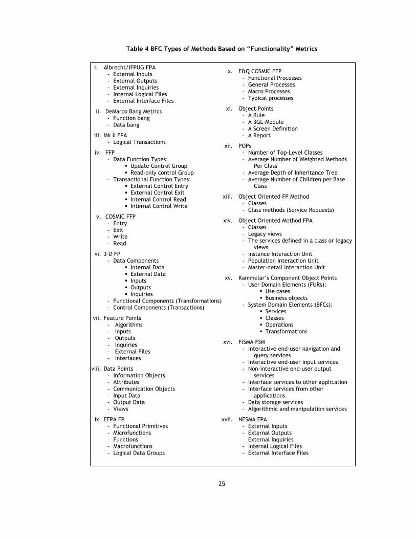
25

Table 4 BFC Types of Methods Based on “Functionality” Metrics

i. Albrecht/IFPUG FPA - External Inputs - External Outputs - External Inquiries - Internal Logical Files - External Interface Files

ii. DeMarco Bang Metrics - Function bang - Data bang

iii. Mk II FPA - Logical Transactions

iv. FFP - Data Function Types:

Update Control Group Read-only control Group

- Transactional Function Types: External Control Entry External Control Exit Internal Control Read Internal Control Write

v. COSMIC FFP - Entry - Exit - Write - Read

vi. 3-D FP - Data Components

Internal Data External Data Inputs Outputs Inquiries

- Functional Components (Transformations) - Control Components (Transactions)

vii. Feature Points - Algorithms - Inputs - Outputs - Inquiries - External Files - Interfaces

viii. Data Points - Information Objects - Attributes - Communication Objects - Input Data - Output Data - Views

ix. EFPA FP - Functional Primitives - Microfunctions - Functions - Macrofunctions - Logical Data Groups

x. E&Q COSMIC FFP - Functional Processes - General Processes - Macro Processes - Typical processes

xi. Object Points - A Rule - A 3GL-Module - A Screen Definition - A Report

xii. POPs - Number of Top-Level Classes - Average Number of Weighted Methods

Per Class - Average Depth of Inheritance Tree - Average Number of Children per Base

Class

xiii. Object Oriented FP Method - Classes - Class methods (Service Requests)

xiv. Object Oriented Method FPA - Classes - Legacy views - The services defined in a class or legacy

views - Instance Interaction Unit - Population Interaction Unit - Master-detail Interaction Unit

xv. Kammelar’s Component Object Points - User Domain Elements (FURs):

Use cases Business objects

- System Domain Elements (BFCs): Services Classes Operations Transformations

xvi. FiSMA FSM - Interactive end-user navigation and

query services - Interactive end-user input services - Non-interactive end-user output

services - Interface services to other application - Interface services from other

applications - Data storage services - Algorithmic and manipulation services

xvii. NESMA FPA - External Inputs - External Outputs - External Inquiries - Internal Logical Files - External Interface Files

26

Since each method has different BFC types, the functional size calculated

by each are expressed in different units; such as “IFPUG FP” in IFPUG FPA,

“Cfsu” in COSMIC FFP, and “MkII FP” in MkII FPA method. EFPA expresses

the size in the same unit as Albrecht FPA and E&Q COSMIC FFP expresses

the size in the same unit as COSMIC FFP. The others -although named also

as FP- are different units, and thus can not be directly compared.

c) Other metrics: These are the other kinds of metrics defined in the

literature. They include, but are not limited to, Web Points, Use Case

Points, etc.

Type of Measures Used. Today there are many metrics being used for software

management activities such as project control and resource allocation during the

development process. Software measurements based on these metrics can be (Hughes,

2000):

a) Direct measures

b) Indirect measures

Direct measurements are taken from a single attribute of an item. For example,

direct measure of size of software code includes LOC. Indirect measurements associate a

measure to an attribute of the object being measured. Functionality is an example of an

indirect measure. The key issue here is that if a measurement is indirect, we need to

examine it more carefully to see if it does genuinely measure some attribute of some

entity (Hughes, 2000).

Software Entity Types Used to Measure “Size” Attribute. Fenton (1996) stated that the

“first obligation of any software measurement activity is identifying the entities and

attributes we wish to measure”, and accordingly he classified them as processes, products,

and resources. Processes are software-related activities. Products are artifacts,

deliverables or documents produced during a software process activity. Resources are the

personnel, materials, tools, and methods required by a process activity. Being a product

attribute, “size” can be measured by using the following entities:

a) Feasibility study document (e.g. number of entities in context diagrams,

etc.)

b) Software Requirements Identification Document (e.g. number of business

process models, data flow diagrams, flow charts, IDEF models, number of

entities in E-R diagrams, etc.)

27

c) Software Requirements Specification Document (e.g. number of pages,

amount of functionality to be delivered to the users, number of

requirements, number of DFDs, etc.)

d) Design Documents (e.g. number of modules, number of bubbles in each

DFD representing module design, number of classes, etc.)

e) Code (e.g. SLOC, Halstead length, Halstead volume, etc.)

Different size measurement methods use different products to measure size of

software. The selected products and thus the measurement methods are strongly related

to measurement timing need (e.g. after software requirements specification is completed,

or after preliminary design) when developing size measurement models.

Suitability for the Software Development Methodology. As the new technologies such as

internet and intranet software, graphical user interfaces, distributed software (e.g. client-

server), and object-oriented systems emerge, new size measurements methods have been

developed and introduced to address the issues related to traditional measurement

methods when applied to those systems. Thus the software size measurement methods can

be classified according to their suitability for the software system development

methodology:

a) Traditional (Structured) Product Development

b) Object Oriented Product Development

c) Web Development

2.3 The Differences between FSM Methods

Among the other size measurement / estimation methods, FSM methods have

become widely used. Currently, four methods have been certified by ISO as international

standards. These are COSMIC FFP (ISO/IEC 19761:2003), IFPUG FPA (ISO/IEC 20926:2003),

Mk II FPA (ISO/IEC 20968:2002) and NESMA FSM (ISO/IEC 24570:2003).

Although all FSM methods measure size by means of the “functionality” delivered

to the users, the main differences between these techniques arise from what they count

and how they do it.

There are a number of studies on the evaluation and comparison of the FSM

methods in the literature. Lother and Dumke (2001) evaluated FSM methods with respect

28

to their suitability for certain functional domains and their maturity as well as discussed

the issues of FSM. In (Demirörs and Gencel, 2004), we evaluated three estimation

methods; Mk II FPA, Jones Very Early Size Predictor, and Early FPA applied early in the life

cycle to a case project (see Section 4.2.1). Rule (1999) discussed the similarities and

differences between IFPUG FPA and Mk II FPA in his study. In another study, Rollo (2000)

discussed the problems associated with sizing web applications and evaluated IFPUG FPA,

Mk II FPA and COSMIC FFP by applying them to a sample e-commerce application.

In this section, we evaluated Mk II FPA, IFPUG FPA and COSMIC FFP being

international ISO standards and depict the differences between these methods. Although

being another FSM method approved by ISO, we have not included NESMA FSM method in

our comparison being very similar to IFPUG FPA.

Figure 1 illustrates the generic measurement process of FSM methods and shows

the differences as well. The main principles of measurement are briefly discussed in the

following paragraphs.

In IFPUG 4.1, the Base Functional Components (BFCs), which are Elementary

Processes (EP), are classified from the end-users view as the Transactional Function Types

and Data Function Types. The Transactional Function Types are also categorized into

External Inputs, External Outputs, and External Inquiries, whereas the Data Functions as;

External Interface Files and Internal Logical Files. Depending on the number of Data

Element Types (DETs) and Record Element Types (RETs) each BFC type contains, these

components are classified as ‘simple’, ‘average’ or ‘complex’. After that weights are

assigned for each BFC. These values are summed up to compute the overall functional

size.

Mk II FPA 1.3.1 aims to measure the information processing amount and uses the

Functional User Requirements (FURs) to measure the functional size. The Base Functional

Components (BFCs) of this method are the Logical Transactions (LTs). A LT is defined as

“the lowest level business processes supported by a software application … triggered by a

unique event of interest in the external world, or a request for information and, when

wholly complete, leaves the application in a self consistent state in relation to the unique

event”. There are no categories of BFCs, i.e. there is only one type of BFC; the LT. The

LTs are identified by decomposing each FUR into its elementary components. Each LT has

three constituents; input, process and output components. The base counts are derived by

counting Input Data Element Types (DETs) for the input component, by counting the Data

Entity Types Referenced for the process component, and by counting the Output DETs for

the output component.

29

Functional UserRequirements

Defined

Identify ElementaryComponents of FURs

Data Movement Types(COSMIC)

E,X,R,W(COSMIC)

Identify BaseFunctional Components

(BFCs)

Classify BFCsinto BFC Types

Determine theBase Counts

Apply MeasurementFunction and Calculate

Functional Size

Functional SizeMeasured

Functional Processes(COSMIC)

Logical Transactions(MkII)

Functional UserRequirements

(FURs)

(# of DETs in the I,# of DETs in the O,

# of referenced PEs )(MkII)

(# of E,# of X,# of R,# of W)

(COSMIC)

FunctionalSize(MkII FP)

FunctionalSize(COSMIC FP)

(Industrial Weightfor I, O, PE)

(MkII)

DeterminePurpose, Scope,Viewpoint & Type

of Count

IdentifyApplication

Boundary of Count

Purpose, Scope,Viewpoint & Type

of Count

ApplicationBoundary of Count

Mk II FPA v.1.3.1

Logical Transactions(MkII)

DetermineContribution

to Functional Size

COSMIC FFP v.2.1

IdentifyData Groups (COSMIC) /Data Entity Types (Mk II)

Data Entity Types(Mk II)

Data Groups(COSMIC)

Data/TransactionFunctions(IFPUG)

TF (EI/EO/EI),DF (EIF/ILF)

(IFPUG)

DetermineComplexity

Elementary Processes(IFPUG)

(#of DETs, #of FTRs) for (EI,EO,EQ),(#of DETs, #of RETs) for (EIF,ILF)

(IFPUG)

FunctionalSize(IFPUG FP)

(Small/Ave./Large)for TFs, DFs

(IFPUG)

Weight for TFs, DFsaccording to complexity

(IFPUG)

IFPUG FPA v.4.1

Data Functions(Files)

Figure 1 FSM Process of IFPUG FPA, Mk II FPA and COSMIC FFP

TF: Transactional Function, DF: Data Function, I: Input, O: Output, PE: Processing Entity, EI: External Input, EO: External Output, EQ: External Query, ILF: Internal Logical File, EIF: External

Interface File, E: Entry, X: Exit, R: Read, W: Write

30

The functionality involved in providing each of these three distinct kinds of

information processing is different. Therefore, the functional size of each LT is computed

by multiplying the size of each component by a weight factor which are calibrated to

industry-average relative effort to analyze, design, program, test and implement these

components in order to enable these three kinds of functionality to be combined into a

single value for a Functional Size. Then, the functional size of each LT is summed up to

compute the functional size of the whole system.

COSMIC FFP Method is designed to measure the functional size of software based

on its FURs as well. In this method, each FUR is decomposed into its elementary

components, called Functional Processes. A Functional Process is defined as “an

elementary component of a set of FURs comprising a unique cohesive and independently

executable set of data movements. Each of these Functional Processes comprises a set of

sub-processes which perform either a data movement or a data manipulation. Since this

method is not designed to measure application domain types which are data manipulation

rich, such as scientific software, the BFCs of this method are assumed to be “Data

Movement Types” only. There are four kinds of data movement types, which are BFC

Types; Entry, Exit, Read, and Write. The functional size of each Functional Process is

determined by counting the Entries, Exits, Reads and Writes in each Functional Process.

Then, the functional sizes of all Functional processes are aggregated to compute the

overall size of the system.

The differences between FSM methods are summarized in Table 5 considering the

following criteria:

- Functional domain applicability. In ISO/IEC 14143-1 (ISO/IEC, 1998), functional

domain is defined as “a class of software based on the characteristics of

Functional User Requirements”. This standard requires that an FSM method

shall describe the functional domain(s) to which the FSM Method can be

applied.

- Unit of measure. ISO/IEC 14143-1 requires that the units in which Functional

Size is expressed shall be defined (ISO/IEC, 1998). “Functional size refers to the

unique size obtained by applying a specific FSM method to a specific set of

software”, meaning that a piece of software has several functional sizes when

measured with different methods. This is due to different types of Base

Functional Components used by different methods.

- Measurement Viewpoint. A viewpoint of Functional User Requirements (FUR) of

software defined when measuring the amount of functionality.

31

- Base Functional Components (BFCs). ISO/IEC 14143-1 requires that an FSM

method shall describe how to identify BFCs within the Functional User

Requirements. BFC is “an elementary unit of FUR defined by and used by an

FSM Method for measurement purposes” (ISO/IEC, 1998).

- BFC Types. “A defined category of BFCs. A BFC is classified as one and only one

BFC Type” (ISO/IEC, 1998). ISO/IEC 14143-1 requires that an FSM method shall

define each BFC type.

- Constituent parts of BFC types. In order to assign numeric values to each BFC,

some of the FSM methods identify and evaluate the constituent parts from

which the BFC types are composed (ISO/IEC, 1998).

- Functionality served by each constituent part. The definitions are taken from

the measurement manuals of IFPUG FPA, Mk II FPA and COSMIC FFP methods.

- Base count derivation. The features that may be counted by each method to

derive functional size.

- Functional complexity weight.

- Relative contribution of base counts to the functional size. Whether the FSM

method give weight to base counts or not when calculating functional size.

32

Table 5 Main Differences between IFPUG FPA, Mk II FPA and COSMIC FFP Methods

IFPUG 4.1

Funct. Domain Applic.

Unit of Measur.

Meas. Viewpoint BFC BFC

Types

Const. Parts of BFC Types

Functionality served by each constituent part

Base Count Deriv.

Funct. Complex. Weight

Relat. Contr.

Small 3

Medium 4 EI Input Message

“An elementary process that processes data or control information that comes from outside the application’s boundary. The primary intent is to maintain one or more ILFs and/or to alter the behavior of the system.”

Count of the number of EIs

Large 6

Small 4

Medium 5 EO Output Message

“An elementary process that sends data or control information outside the application’s boundary. The primary intent is to present information to a user through processing logic (at least one mathematical formula or calculation, or create derived data) other than or in addition to the retrieval of data or control information.”

Count of the number of EOs

Large 7

Small 3

Medium 4

Any domain

IFPUG FP End User EP TF

EQ An Input/ Output Pair

“An elementary process that sends data or control information outside the application boundary. The primary intent of an external inquiry is to present information to a user through the retrieval of data or control information. “

Count of the number of EQs

Large 6

Table 5 Main D

ifferences between IFPU

G FPA

, Mk II FPA

and COSM

IC FFP Methods

33

Table 5 Main Differences between IFPUG FPA, Mk II FPA and COSMIC FFP Methods (continued)

IFPUG 4.1

Funct. Domain Applic.

Unit of Measur.

Meas. Viewpoint BFC BFC

Types

Const. Parts of BFC Types

Functionality served by each constituent part

Base Count Deriv.

Funct. Complex. Weight

Relative Contr.

Small 7

Medium 10

ILF

Retained Data maintained by the application

“A user identifiable group of logically related data or control information maintained within the boundary of the application. The primary intent is to hold data maintained through one or more elementary processes of the application being counted.”

Count of the number of ILFs

Large 15

Small 5

Medium 7

Any domain

IFPUG FP

End User EP DF

EIF

Retained Data maintained by some other application

“A user identifiable group of logically related data or control information referenced by the application, but maintained within the boundary of another application. The primary intent is to hold data referenced through one or more elementary processes within the boundary of the application counted.”

Count of the number of EIFs

Large 10

Table 5 Main D

ifferences between IFPU

G FPA

, Mk II FPA

and COSM

IC FFP Methods

(cont.)

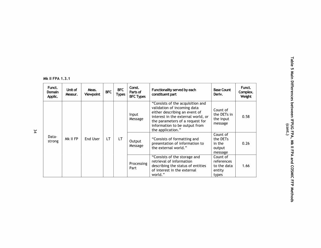
34

Table 5 Main Differences between IFPUG FPA, Mk II FPA and COSMIC FFP Methods (continued)

Mk II FPA 1.3.1

Funct. Domain Applic.

Unit of Measur.

Meas. Viewpoint BFC BFC

Types

Const. Parts of BFC Types

Functionality served by each constituent part

Base Count Deriv.

Funct. Complex. Weight

Input Message

“Consists of the acquisition and validation of incoming data either describing an event of interest in the external world, or the parameters of a request for information to be output from the application.”

Count of the DETs in the input message

0.58

Output Message

“Consists of formatting and presentation of information to the external world.”

Count of the DETs in the output message

0.26

Data- strong Mk II FP End User LT LT

Processing Part

“Consists of the storage and retrieval of information describing the status of entities of interest in the external world.”

Count of references to the data entity types

1.66

Table 5 Main D

ifferences between IFPU

G FPA

, Mk II FPA

and COSM

IC FFP Methods

(cont.)

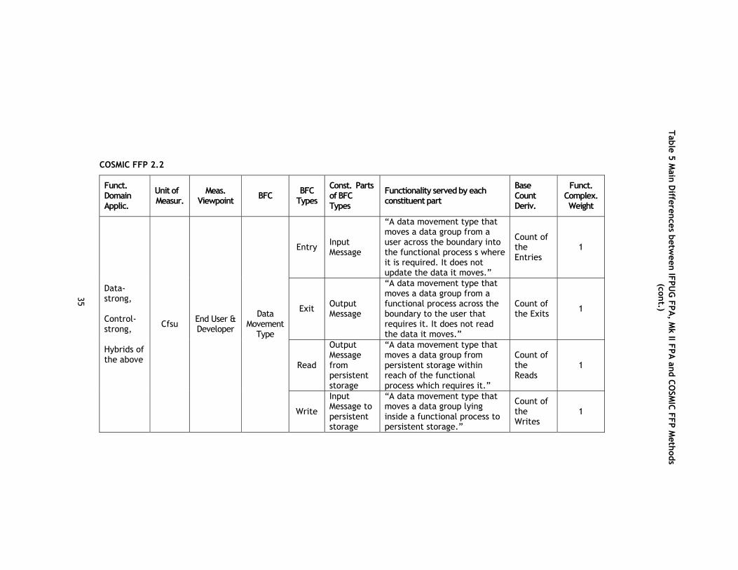
35

Table 5 Main Differences between IFPUG FPA, Mk II FPA and COSMIC FFP Methods (continued)

COSMIC FFP 2.2

Funct. Domain Applic.

Unit of Measur.

Meas. Viewpoint BFC BFC

Types

Const. Parts of BFC Types

Functionality served by each constituent part

Base Count Deriv.

Funct. Complex. Weight

Entry Input Message

“A data movement type that moves a data group from a user across the boundary into the functional process s where it is required. It does not update the data it moves.”

Count of the Entries

1

Exit Output Message

“A data movement type that moves a data group from a functional process across the boundary to the user that requires it. It does not read the data it moves.”

Count of the Exits 1

Read

Output Message from persistent storage

“A data movement type that moves a data group from persistent storage within reach of the functional process which requires it.”

Count of the Reads

1

Data-strong, Control-strong, Hybrids of the above

Cfsu End User & Developer

Data Movement

Type

Write

Input Message to persistent storage

“A data movement type that moves a data group lying inside a functional process to persistent storage.”

Count of the Writes

1

Table 5 Main D

ifferences between IFPU

G FPA

, Mk II FPA

and COSM

IC FFP Methods

(cont.)

36

2.4 Discussion of the Literature Survey Results

Software measurement and estimation are among the important practical

problems in software engineering. Poor management usually results in runaway projects

that spiral out of control. In many cases, projects become runaways, and as a result the

measurement targets to which they are being managed were largely unreal to begin with.

It seems like numerous size measurement methods are still considered as “immature” by

many people in the industry. Size measurement metrics and methods that have been

defined have not been able to solve the problem. The problem partially lies in the fact

that, despite the various approaches to software size measurement, there are still many

issues of existing metrics and methods.

First, global standards on procedures and methods for metric definitions and usage

are lacking or do not exist at all. Experts disagree on what should be counted and how the

counting should happen (Glass, 2002). A structured measurement process should be

defined and a standard guideline, such as a measurement manual, must be produced. This

will ensure that for all projects, consistent and reliable size estimates can be made by

different users.

The details of some measurement methods and metrics; such as Object Points

(Banker et al., 1994), 3-D Function Points (Whitmire, 1992), Predictive Object Points

(Teologlou, 1999) have not been published. Therefore too little is known about their

validity. Another example is LOC; with this metric, the size of a final software product can

be defined in no less than eleven different ways (Bennet, 1996).

Second issue which is related to counting standards and procedures arises from the

differences between the versions of the same method. For example, IFPUG FPA practices

have different versions (Release 3.0 vs. 4.1). These differences are stated to reduce a

project’s FP point count by an average of 26%, and thus, limit the size comparisons

between recent projects and past projects (Bennet, 1996).

Thirdly, validation of many metrics and measurement models is also insufficient. In

the past, validation has been a relaxed process, sometimes relying on the credibility of the

proposer, rather than on rigorous validation procedures (Fenton, 1996). However, both the

metric and the measurement model should be valid. That is, the defined metric should

accurately characterize the “size” attribute it claims to measure and the measurement

37

model should make accurate predictions by comparing model performance with known

data. The method should obey the principles and rules of the measurement theory so that

correct arithmetic operations and statistical analysis can be done on the results obtained

(Fenton, 1994; 1996).

Due to these reasons most of the existing metrics defined lack necessary

measurement properties and the rigor, which is available in other engineering disciplines.

The estimators in other engineering disciplines use construction standards and

architectural drawings to assess the size of the final product and to aid in developing

initial project size very early in the development process. However, the software

engineering field lacks such architectural form to assist estimators.

Another important factor of “immaturity of measurement” is measurement timing.

The software estimates should be performed at the beginning of the life cycle to be able

to respond to contracts and plan in advance. This is the time when we do not yet know the

sufficient details of the problem. Meli et al. (2000) described this situation as a paradox:

Size estimation would be necessary when we do not have enough information and early

measurement methods to obtain it. When we can measure with the greatest accuracy, we

do not need that information for effort and duration prediction purposes any more. In

fact, most of the recent researches have concentrated on the later phases of software

development (at least a software requirements specification document and in many cases

a preliminary design) when developing size measurement models. There are few size

estimation methods which are developed especially for early estimation. EFPA (Meli,

1997a; Meli, 1997b; Conte et. al., 2004) and E&Q COSMIC FFP (Meli et al., 2000; Conte et.

al., 2004) are the examples of such methods.

One of the most significant issues of software size measurement is that the

measurement methods have unclear conceptual and theoretical basis. Software

development practitioners do not have socially accepted basic size measures or on what

constitutes product size. There is a lack of good empirical relational systems and the

software attributes (Hughes, 2000). In addition, the mappings from the real world domain

to the metric models are usually not well defined. Therefore, Fenton (1994; 1996) called

for a rigor in software engineering through measurement theory. The problems of function

points related to scale types defined in measurement theory were also summarized by

Kitchenham (1997). Xia (1998) suggested that clear definition of basic software concepts

before developing any serious measures was a basic requirement for any scientific

theories. As for software size, understanding of this attribute of software has become a

concept which is related to other attributes such as; the length of the code, functionality

38

delivered to the users, amount of reuse and complexity of the development (Fenton, 1996;

Poel, 1998). However, there are still arguments on the meaning of the terms “size”,

“length”, “complexity, and “functionality”.

Some studies have been started on the conceptual and theoretical basis of

measurement methods. Lokan (1999) studied the correlations between the BFC types in

FPA. A large data set - International Software Benchmarking Standard Group (ISBSG)

dataset was analyzed in this study to gain further insight into the correlations. ISBSG is one

of several opportunities that currently exist for gathering, retrieving, and sharing industry

data (Garmus, 2002). These kinds of data sets give opportunity to study not only the

conceptual and theoretical basis but the validations of both the existing methods and the

ones to be developed.

Another study on this issue was initiated by ISO. ISO started to work on FSM to

establish common principles of the methods based on “functionality” metric and brought a

consistent terminology for the concepts related to size. ISO/IEC 14143 standard will also

provide a framework for verifying repeatability and reproducibility as well as for accuracy

for the methods based on “functionality” (Lother and Dumke, 2001).

Kitchenham and Kansala (1993); Jeffery and Stathis (1996); and Lokan (1999)

studied the correlations between the BFC types in FPA. Although some of their findings

agree, they found out different correlations in others. The outcomes of these studies

showed that the presence of these correlations cause to count the same things more than

once in FPA. Moreover, Kitchenham (1997) stated that the different results of studies on

correlations showed that, any predictive model based on the sum of the elements would

not be stable for different datasets.

Another important issue of size measurement is the convertibility of the measures

obtained by different methods and metrics to each other. There are various size

measurement methods addressing different software domains. Thus, for the comparison

purposes of one or more methods, convertibility of the results has to be considered

(Lother and Dumke, 2001, Symons, 2001).

There are some studies to define the convertibility of functional size, measured by

different FSM methods. Symons (1999) studied on the convertibility of Mk II FP and IFPUG

FP to each other, and gave a formula by examining the relationships between the BFC

types in Mk II FPA and IFPUG FPA. In (COSMIC, 2003), it is stated that there are practical

and theoretical reasons why convertibility of size is difficult; these are the lack of enough

39

data to develop statistically-based conversion formulae and having no definite conceptual

mapping between the BFC’s of one method and of the other to develop an exact

mathematically-based conversion formula.

This chapter presented a survey of literature concerning size measurement metrics

and methods and a discussion on them. So, what trends can be observed from the current

literature? Still a lot of research is necessary to deal with the conceptual and theoretical

basis of measurement methods, convertibility of size estimates made by different methods

and the automation of the existing methods. In addition, although there designed a

number of methods to measure algorithmic and scientific software such as De Marco’s

Bang Metrics (DeMarco, 1982), Feature Points (Jones, 1987), ASSET-R (Reifer, 1990) and 3-

D Function Points (Whitmire, 1992), none of them have been certified by ISO as an

international standard. And it is for sure that early size estimation is an area demanding

further research. New methods, metrics and guidelines are required to make accurate size

estimations early in the life cycle as well as studies to validate the suggested metrics and

models.

40

CHAPTER III

3 A NEW FSM METHOD: ARCHI-DIM FSM

“Everything should be made as simple as possible, but not simpler” Albert Einstein

3.1 Overview

Based on the findings of the literature review and the results of the case studies

we performed, we identified a number of improvement opportunities for FSM methods

(see Section 5.1.1). This chapter does not attempt to analyze all of them in depth and

make suggestions for all, but rather we focus on two of the significant improvement

opportunities, which are related to the conceptual and theoretical basis of FSM and

extension of the applicability of these methods to different software functional domain

types.

The existing FSM methods have been used for more than twenty years. In spite of

the fact that there still exist some improvement opportunities, they give satisfactory

results most of the time. Therefore, while suggesting improvements for FSM, we take this

fact into account and make use of the concepts defined by the methods which we find

valuable.

After discussing our approach on how to improve the conceptual and theoretical

basis of FSM methods, we present a new FSM method, called ARCHItectural DIMensions

Based FSM (ARCHI-DIM). The Measurement Guidelines of this new method is prepared to be

conformant to ISO/IEC 14143-1, the International Standard for FSM, and is given in Section

3.3.2 of this chapter.

41

3.2 The Need for a New Approach for Counting Software Functional Size

In this thesis study, we focus on the “additivity” of the functional sizes of different

BFC Types. In FSM, we want to measure the “functional size” attribute of software.

Traditionally, this is a single value obtained by a specific FSM method. Abran (1994) stated

the problem for IFPUG FPA as “The additivity of functions poses a question, namely the

relevance of adding elements which are of different types and mean different things”.

Thus, he suggested that it would be more appropriate to call the final result an index

rather than a measurement of the size of an application and the FP count could be used as

a measurement or measurements of size able to reflect various points of view with

different units. These dimensions in one or several subsets could be used to define and

measure functional size of software.

While discussing indirect measures, Fenton suggested “using vectors of measures

with rules for combining the vector elements into a larger, indirect measure” (Fenton,

1997). Kitchenham (1997) also mentioned the problem of additivity and suggested not

adding or combining the resulting counts together, instead using basic counts that are not

weighted as a vector of measures that describe the system”; such as a person’s clothing

size is defined as “chest size”, “waist size”, and “hip size”.

In fact, if we look at other engineering disciplines, the sizes of products are

pronounced as a vector of measures most of the time. This is analogous to estimating

effort and cost of a construction in civil engineering. An example from Civil Engineering

Standard Method of Measurement (CESMM, 1991) is Motorway Construction. The related

processes (work items) performed to build a motorway are categorized as:

- Outfall (excavation (m3), filling (m3), concrete (m3), pipe work (m))

- Sewers (pipelines (m), manholes number))

Therefore, when we talk about the size of a motorway, we are talking about the

size of constituent parts of it in different units. The effort and cost related to the sizes of

each item used and the related effort to perform each process to construct that part are

given in this manual.

Similarly, the size of a building is a vector of measures of the number of floors and

square foot base area of the building, the number of rooms in a house, etc. rather than a

42

single value. When finding the size of a building, we do not add or multiply the base area

of the building with the number of floors.

However, that is exactly what we do in software engineering practice. If vectors of

measures for functional size could be defined by identifying the different types of

functionality, another contribution might be that the effort and cost associated with each

could be estimated separately as in civil engineering practice. Experimental studies can

be conducted to find the correlation between the size of each functionality type and the

effort needed to develop that type of functionality which can pioneer new effort

measurement methods.

Since effort and cost for each component can be estimated in the same units, say

person-hours / dollars, respectively; after effort and cost estimation, adding these values

to estimate the overall effort and cost required will not cause any problem with respect to

measurement theory which is a significant issue in software FSM.

Clear definition of basic concepts is a basic requirement for any scientific theory

before developing any serious measure (Xia, 1998). Therefore, first we should clarify the

definition of the functionality concept before defining vectors of measures for functional

size. Some of the definitions related to functionality we found in the literature are as

follows:

- “Functionality: Waffle for "features" or "function". The capabilities or behaviors

of a program, part of a program, or system, seen as the sum of its features"

(Computing Dictionary, 2005).

- “Functionality captures an intuitive notion of the amount of function contained

in a delivered product or in a description of how the product is supposed to be”

(Fenton, 1996).

- “Functional size is a measure of the quantity of information processing

functionality the customer requires of the software independent of the

technology used” (Rule, 2001).

By the introduction of ISO/IEC 14143-1 standard on FSM, the “size” and “functional

size” concepts are differentiated. In ISO/IEC 14143-1 (1998), the definitions of concepts

related to functionality are given as:

- Functional Size: “a size of the software derived by quantifying the Functional

User Requirements”.

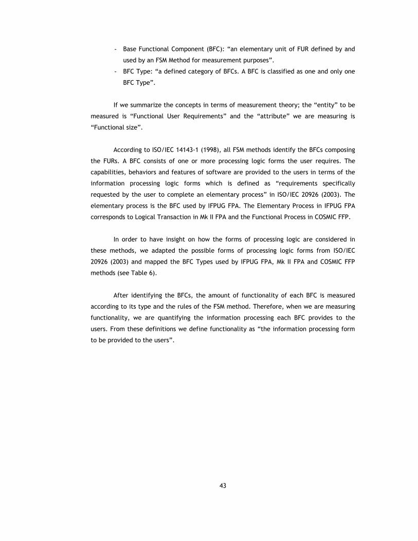
43

- Base Functional Component (BFC): “an elementary unit of FUR defined by and

used by an FSM Method for measurement purposes”.

- BFC Type: “a defined category of BFCs. A BFC is classified as one and only one

BFC Type”.

If we summarize the concepts in terms of measurement theory; the “entity” to be

measured is “Functional User Requirements” and the “attribute” we are measuring is

“Functional size”.

According to ISO/IEC 14143-1 (1998), all FSM methods identify the BFCs composing

the FURs. A BFC consists of one or more processing logic forms the user requires. The

capabilities, behaviors and features of software are provided to the users in terms of the

information processing logic forms which is defined as “requirements specifically

requested by the user to complete an elementary process” in ISO/IEC 20926 (2003). The

elementary process is the BFC used by IFPUG FPA. The Elementary Process in IFPUG FPA

corresponds to Logical Transaction in Mk II FPA and the Functional Process in COSMIC FFP.

In order to have insight on how the forms of processing logic are considered in

these methods, we adapted the possible forms of processing logic forms from ISO/IEC

20926 (2003) and mapped the BFC Types used by IFPUG FPA, Mk II FPA and COSMIC FFP

methods (see Table 6).

After identifying the BFCs, the amount of functionality of each BFC is measured

according to its type and the rules of the FSM method. Therefore, when we are measuring

functionality, we are quantifying the information processing each BFC provides to the

users. From these definitions we define functionality as “the information processing form

to be provided to the users”.

44

Table 6 Forms of Processing Logic Performed by BFC Types of FSM Methods

IFPUG BFCs MkII BFCs COSMIC BFCs LT Data Movement Forms of Processing Logic** EI EO EQ I PE O E X R W

Acquisition of data or control information that enters the application boundary m c c X X Validation of acquired data or control information entered from outside of the application boundary to the inside of the boundary

c c c X X

Preparation and formatting information to be presented outside the application boundary to the Interfacing Entities.

c m m X X

Presenting information outside the application boundary to the Interfacing Entities.

c m m X X

Maintaining “groups or collections of related and self-contained data“ (Entity Types/Data Groups/Data Classes/Objects of interest) in permanent storage

m* m* n X X

Retrieving data from “one or more groups or, collections of related and self-contained data” from permanent storage which may be internal or external to the application.

c c m X X

Creating derived data c m* n X X Resorting or rearranging a set of data read from or to be written to permanent storage

c c c X X

Filtering and selecting of data by using specific criteria to compare multiple sets of data read from to or to be written to permanent storage

c c c X X

Controlling the behavior of the system (alter, read) m* m* n X X Conversions of equivalent values c c c X X X X Analyzing conditions to determine which are applicable c c c X X X Performing mathematical operations and calculations c m* n X X X

** : adapted from (ISO/IEC 20926, 2003) m: it is mandatory that the BFC type perform the form of processing logic ; m*: it is mandatory that the BFC type perform at least one of these (m) c: the BFC type can perform the form of processing logic, but it is not mandatory; n: BFC type cannot perform the form of processing logic X: The constituent part of BFC type performs the form of processing logic; EI: External Input; EO: External Output; EQ: External Inquiry; I: Input; PE: Processing Entity; O: Output;E: Entry; X: Exit; R: Read; W: Write.

Table 6 Forms of Processing Logic Perform

ed by BFC Types of FSM M

ethods

45

After clarifying the definition of “functionality”, we can define vectors of

measures for functional size. Different BFC Types means that we want to measure

different types of functionalities software provides to its users. If the related forms of

processing logic are grouped into functionality types, then it is possible to define vectors

of measures and BFC Types for each.

Therefore, we take the list of all forms of processing logic that can be requested

by the users given in the manual of IFPUG FPA 4.1, and then we mapped BFC types of Mk II

FPA and COSMIC FPA methods to this list in order to understand better the BFC types and

their constituent parts in relation to the kinds of processing logic met by each of them

(see Table 6). This gives us insight on the forms of processing logic and which of them can

not be sized by the existing FSM methods. In fact, this is a bottom-up approach for

identifying different types of functionality.

We also approached this problem in a top-down fashion considering the software

functional domain types and the components of the software architecture.

We took into account the software functional domain types when categorizing the

functionality types since different forms of processing logic are utilized in different

software functional domain types. The software functional domain types are classified as

data strong systems (e.g. MIS), control strong systems (e.g. telecommunications software),

function strong systems (e.g. scientific software) and hybrids of these three types (see

Section 2.2.2).

A number of studies, which depict the differences between the forms of processing

logic in different functional domain types, exist in the literature.

DeMarco (1982) classified the systems into three groups: function-strong, data-

strong and hybrid systems and defined his bang metrics according to this classification.

Reifer (1991) took into account the characteristics of different types of functional

domain types such as the scientific field and the real time field in addition to MIS field

while constructing his method ASSET-R. He classified the characteristics by field of

application as given in Table 7 (Abran, 1994b).

Maya et.al. (1998) discussed the differences between the forms of processing logic

in data-strong and real-time systems and developed their FFP method considering these

differences. One major difference is found to be the variation in the number of sub-

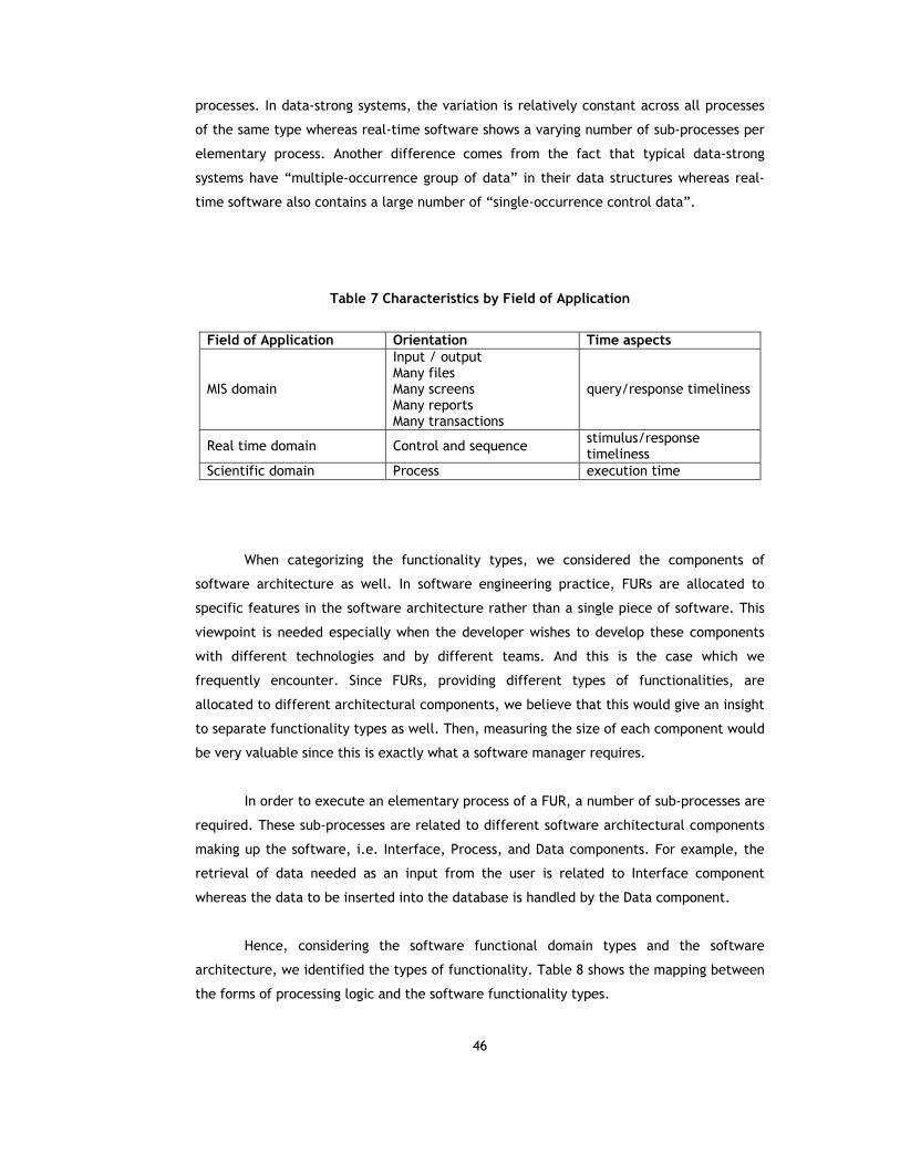
46

processes. In data-strong systems, the variation is relatively constant across all processes

of the same type whereas real-time software shows a varying number of sub-processes per

elementary process. Another difference comes from the fact that typical data-strong

systems have “multiple-occurrence group of data” in their data structures whereas real-

time software also contains a large number of “single-occurrence control data”.

Table 7 Characteristics by Field of Application

Field of Application Orientation Time aspects

MIS domain

Input / output Many files Many screens Many reports Many transactions

query/response timeliness

Real time domain Control and sequence stimulus/response timeliness

Scientific domain Process execution time

When categorizing the functionality types, we considered the components of

software architecture as well. In software engineering practice, FURs are allocated to

specific features in the software architecture rather than a single piece of software. This

viewpoint is needed especially when the developer wishes to develop these components

with different technologies and by different teams. And this is the case which we

frequently encounter. Since FURs, providing different types of functionalities, are

allocated to different architectural components, we believe that this would give an insight

to separate functionality types as well. Then, measuring the size of each component would

be very valuable since this is exactly what a software manager requires.

In order to execute an elementary process of a FUR, a number of sub-processes are

required. These sub-processes are related to different software architectural components

making up the software, i.e. Interface, Process, and Data components. For example, the

retrieval of data needed as an input from the user is related to Interface component

whereas the data to be inserted into the database is handled by the Data component.

Hence, considering the software functional domain types and the software

architecture, we identified the types of functionality. Table 8 shows the mapping between

the forms of processing logic and the software functionality types.

47

Table 8 Forms of Processing Logic and Software Functionality Types

Forms of Processing Logic Software Functionality Types Acquisition of data or control information that enters the application boundary Interface Functionality Validation of acquired data or control information entered from outside of the application boundary to the inside of the boundary Interface Functionality

Preparation and formatting information to be presented outside the application boundary to the Interfacing Entities. Interface Functionality

Presenting information outside the application boundary to the Interfacing Entities. Interface Functionality

Maintaining “groups or collections of related and self-contained data“ (Entity Types/Data Groups/Data Classes/Objects of interest) in permanent storage

Permanent Data Access/Storage Functionality

Retrieving data from “one or more groups or, collections of related and self-contained data” from permanent storage which may be internal or external to the application.

Permanent Data Access/Storage Functionality

Creating derived data Permanent Data Access/Storage Functionality

Resorting or rearranging a set of data read from or to be written to permanent storage

Permanent Data Access/Storage Functionality

Filtering and selecting of data by using specific criteria to compare multiple sets of data read from to or to be written to permanent storage

Permanent Data Access/Storage Functionality

Control the behavior of the system (alter, read) Control Process Functionality

Conversions of equivalent values Algorithmic / Data Manipulation Process Functionality

Analyzing conditions to determine which are applicable Algorithmic / Data Manipulation Process Functionality

Performing mathematical operations and calculations Algorithmic / Data Manipulation Process Functionality

Table 8 Forms of Processing Logic and Softw

are Functionality Types

48

The types of software functionalities identified are the following;

- Interface Functionality: Involves the functionalities provided to an interfacing

entity – a person who enters and receives output or automated user (another

software or automatic data collection device) that move data in/out of a

process via an interface.

- Business Process Functionality: may be of two types depending on the software

functional domain. A hybrid software system may have more than one of these

process functionality types:

- Control Process Functionality: Involves the functionalities provided to an

interfacing entity to control the behaviour of a system.

- Algorithmic / Data Manipulation Process Functionality: Involves the

functionalities provided to transform data item to create another one by means

of mathematical and/or logical operations.

- Permanent Data Access/Storage Functionality: Involves the functionalities

provided to an interfacing entity to access (read, write) Permanent group or

collection of related and self-contained data in the real world. These “groups

or collections of related and self-contained data” are often called as entity

types, data groups, data classes or objects of interest, depending on the

terminology of the development environment.

3.3 ARCHI-DIM FSM Method and the Measurement Guidelines

3.3.1 Introduction

ARCHItectural DIMensions Based Functional Size Measurement (ARCHI-DIM FSM)

Method is developed to measure the functional size of software systems. It measures the

Functional User Requirements (FURs) and quantifies different types of functionalities

delivered to the users. This section explains the rules of ARCHI-DIM FSM Method and gives

the measurement guidelines.

ARCHI-DIM FSM Method is intended to comply with ISO/IEC 14143-1 - the

International Standard for Functional Size Measurement. The measurement guidelines are

prepared according to the concepts and rules of this standard.

49

3.3.1.1 Uses of Functional Size Measurement

ARCHI-DIM FSM Method can be used for project management activities such as

tracking the progress of a project, and managing scope change or estimation and

performance management.

3.3.1.2 Functional Domain Applicability

ARCHI-DIM is designed to be applicable to measure application software from the

domain of data-strong, control-strong, function-strong and hybrid systems.

- Data strong systems: Often characterized by the need to manage large amounts

of data. Financial transaction process/accounting and banking software are

some examples.

- Control strong systems: Often characterized by the need to control events that

changes the behavior of a system. Telecommunications software and embedded

software for machine control (such as lifts) are some examples.

- Function strong systems: Characterized by complex mathematical algorithms

and rules. Scientific software and expert systems are some examples.

- Hybrid systems: These systems are hybrids of two or more of the above

systems. Defense related systems or real-time reservation systems for hotels

are some examples.

3.3.1.3 ARCHI-DIM Measurement Process

ARCHI-DIM Measurement process is shown in Figure 2. The activities of the

measurement process are given in detail in Section 3.3.1.5.

3.3.1.4 Estimation Timing

ARCHI-DIM can be applied as soon as the Functional User Requirements (FURs) are

defined.

50

Identify ElementaryProcesses within FURs

Identify BFC Types ofthe Constituent Parts

of Elementary Processes

Determine theBase Counts

CalculateFunctional Size by

Applying MeasurementFunction

Functional SizeMeasured

Functional UserRequirements

(FURs)Determine

Purpose, Type, Scope,and Viewpoint

of Count

Identify ApplicationBoundary of

Measurement

Purpose, Scope,Viewpoint & Type

of Count

ApplicationBoundary of Measurement

Elementary Processes(ARCHI DIM)

InterfaceFunctionalities(ARCHI DIM)

Process (Algorithmic)Functionalities

(ARCHI DIM)

Pers. Data Acc./Strg.Functionalities

(ARCHI DIM)

Int. Funct.(RI/O, WI/O, RVS, WVS)

(ARCHI DIM)

Process(Control) Funct.

(RVS, WVS)(ARCHI DIM)

Pers. DataAcc./Strg. Funct.

(RPS, WPS, RVS, WVS)(ARCHI DIM)

Process(Algorithmic) Funct.

(RVS, WVS)(ARCHI DIM)

Int. Funct.(# of DETs in

RI/O, WI/O, RVS, WVS)(ARCHI DIM)

Pers. Data Acc/Str.Func.(# of DETs in

RPS, WPS, RVS, WVS)(ARCHI DIM)

Process(Algorithmic) Funct.

(# of DETs inRVS, WVS)

(ARCHI DIM)

Process(Control) Funct.

(# of DETs inRVS, WVS)

(ARCHI DIM)

InterfaceFunctionalSize(ARCHI DIM)

Process (Control)FunctionalSize(ARCHI DIM)

Process (Alg.)FunctionalSize

(ARCHI DIM)

Pers. DataAcc./Strg.

FunctionalSize(ARCHI DIM)

Process (Control)Functionalities(ARCHI DIM)

Functional UserRequirements

Defined

Identify the FURswithin the Scope ofthe Measurement

FURs withinthe Scope of

the Measurement

Identify Data Groups Identify DataElement Types (DETs)

DETsData Groups

Identify Constituent Partsof Elementary Processes

Figure 2. ARCHI-DIM Measurement Process

RI/O: Read from I/O Device, WI/O: Write to I/O Device, RVS: Read from Volatile Storage, WVS: Write to Volatile Storage, RPS: Read from Permanent Storage, WPS: Write to Permanent Storage

51

3.3.1.5 Degree of Convertibility

The convertibility of functional sizes obtained by ARCHI-DIM to the functional sizes

obtained by other FSM methods has not been studied yet. However, in Section 4.2.3.4,

the relationship of the BFC Types of ARCHI-DIM FSM with the BFC Types of Mk II FPA and

COSMIC FFP methods are discussed. The measurement results of a case study by these

methods are compared. This study would be helpful in finding a conversion formula

between these methods. More case studies shall be conducted in order to find the degree

of convertibility of the functional sizes obtained by this method in the future.

3.3.1.6 Glossary

This thesis study makes use of the definitions of ISO/IEC 14143-1 (1998). Therefore, the

glossary is prepared according to the definitions of this standard.

Application Boundary: a conceptual interface between the software under study and its

Interfacing Entities.

Base Functional Component (BFC): an elementary unit of Functional User Requirements

defined by and used by an FSM Method for measurement purposes.

BFC Type: a defined category of BFCs. Examples of BFC Types are 'External Inputs',

'External Outputs' and 'Logical Transactions', 'Internal Logical Files', etc.

FSM Method: a specific implementation of FSM defined by a set of rules, which conforms to

the mandatory features of ISO/IEC 14143-1 (1998).

Functional Domain: a class of software based on the characteristics of Functional User

Requirements which are pertinent to FSM.

Functional Size: a size of the software derived by quantifying the Functional User

Requirements.

Functional Size Measurement: the process of measuring Functional Size.

52

Functional User Requirements: a sub-set of the user requirements. The Functional User

Requirements represent the user practices and procedures that the software must perform

to fulfill the users’ needs. They exclude Quality Requirements and any Technical

Requirements.

Interfacing Entity: a person or automated user (another software or automatic data

collection device) that move data in/out of a process via an Interface.

Quality Requirements: any requirements relating to software quality as defined in ISO 9126

(1991).

Technical Requirements: requirements relating to the technology and environment, for the

development, maintenance, support and execution of the software.

User: any person that specifies Functional User Requirements and/or any person or thing

that communicates or interacts with the software at any time.

3.3.2 ARCHI-DIM Measurement Process - The Method and the Rules

The steps of ARCHI-DIM FSM Method measurement process are discussed in the

following sub-sections.

3.3.2.1 Determining the Purpose of Measurement

At the beginning of measurement process, it is essential that the purpose of

measurement is defined, i.e. why the measurement is being done and where the

measurement results would be used. The application boundary of software is determined

according to the purpose of the measurement.

The example purposes of measurement may be:

- to provide functional size as an input to effort and cost estimation models, or

productivity analysis,

- to help project tracking and control,

- to compare the amount of functionality delivered by different software,

- to learn an organization’s software portfolio etc.

53

3.3.2.2 Determining the Type of Measurement

There are three types of measurement:

- Measurement of development projects: measures the amount of functionality

to be provided to the users when the project is complete.

- Measurement of enhancement projects: measures the amount of functionality

in the modifications (add, change, or delete) to the existing application when

the project is complete.

These two types of measurement may have the purposes of project management,

project forecasting and control.

Measurement of applications: measures the amount of current functionality an

application provides to the users. This type of measurement may have the purposes of

comparing the amount of functionality delivered by different software or learning an

organization’s software portfolio for the purpose of asset valuation, etc.

3.3.2.3 Determining the Scope of Measurement

After determining the purpose of measurement, the measurement scope shall be

determined in order to identify which FURs will be included in the measurement process.

For example, if an organization needs to know the size of its software portfolio,

then the scope of the measurement will include all the FURs currently utilized. However,

if a project manager is seeking to determine the work-output of a particular group of

developers, the scope includes the FURs that this group has developed. Therefore, the

scope of measurement is closely related with the purpose and type of measurement.

3.3.2.4 Identifying Application Boundary of Count

After determining the purpose, type and scope of measurement, the application

boundary of count shall be identified. The application boundary defines the conceptual

border between the software and the ‘Interfacing Entities’. Therefore, it determines what

functionality is included and what is excluded in the measurement.

54

‘Input data’ from the interfacing entities crosses the boundary and enters the

application. ‘Output data’ leaves the application and crosses the boundary to reach the

interfacing entity. The functionality types, the sizes of which are to be measured, lies

within the application boundary.

3.3.2.5 Mapping of Functional User Requirements (FURs) to ARCHI-DIM Model

Representation condition of Measurement Theory requires that every measure

should be associated with a model of how the measure maps the entities and attributes in

the real world to the elements of a numerical system (Fenton, 1996). After determining

the purpose, type, scope, viewpoint of measurement and boundary of count, the FURs are

mapped to ARCHI-DIM model for measuring the functional size of each FUR.

The construction of ARCHI-DIM model includes:

- Identifying the FURs within the boundary of count

- Identifying BFCs within FURs

- Identifying Data Groups

- Identifying Data Element Types (DETs)

- Identifying the Constituent Parts of BFCs

- Identifying the BFC Types of the Constituent Parts of BFCs

These activities are explained in the following sub-sections.

Identifying FURs within the Scope of the Measurement

The FURs to be included in the FSM process includes the ones that are inside the

application boundary of count. The FURs that are outside of the application boundary of

count are excluded.

Identifying Base Functional Components (BFCs) within FURs

In this step, the BFCs within the FURs are identified. The BFCs of ARCHI-DIM are

“Elementary Processes”. An Elementary Process is an elementary unit of Functional User

Requirements supported by the application and that is meaningful to the user(s). It is

triggered by a unique event that is of interest to the user. It is complete when it has

executed all that is required to be done in response to the triggering event.

55

Identifying Data Groups

Next step is to identify the data groups which are “the groups or collections of

related and self-contained data about which the user wants to hold information”. These

may be called as data entity types, data classes or objects of interest, depending on the

terminology used in the development environment. Data groups may have different forms

in a piece of software:

- Data groups on I/O device (display screen, printed report, control panel

display, keyboard, mouse, printer, interface with other applications or driver

of other devices)

- Data group in volatile storage (data structure allocated dynamically or through

a pre-allocated block of memory space)

- Data group in permanent storage (file, database table, ROM memory, etc.)

Identifying Data Element Types (DETs)

After determining the data groups, the DETs which hold information about data

groups (or the attributes of data groups) shall be identified. (e.g., ‘Employee name’ is a

DET which holds information about the employee data group). The reason of identifying

DETs is that the number of DETs would be used as base counts when measuring the size of

BFC Types.

Identifying the Constituent Parts of BFCs

In ARCHI-DIM FSM, three constituent parts of BFCs, which serve different

functionalities, are defined. These are:

- Interface: Involves the functionalities provided to an interfacing entity – a

person who enters and receives output or automated user (another software or

automatic data collection device) that move data in/out of a process via an

interface.

- Business Process: may be of two types depending on the software functional

domain. A hybrid software system may have more than one of these process

functionality types:

o Control Process: Involves the functionalities provided to an interfacing

entity to control the behavior of a system.

56

o Algorithmic / Data Manipulation Process: Involves the functionalities

provided to transform data item to create another one by means of

mathematical and/or logical operations.

- Permanent Data Access/Storage: Involves the functionalities provided to an

interfacing entity to access (read, write) permanent group or collection of

related and self-contained data in the real world. These “groups or collections

of related and self-contained data” are often called as entity types, data

groups, data classes or objects of interest, depending on the terminology of the

development environment. In ARCHI-DIM, it is called as Data Group.

An Elementary Process may involve one or more constituent parts. For example, if

an Elementary Process is “Adding customer information to the database”, this Elementary

Process involves Interface functionalities and Permanent Storage Data Access/Storage

functionalities. In data-strong systems, most of the Elementary Processes involve these

kinds of functionalities. In real-time systems, Control Process functionalities are also

present. If the software system is a scientific one, Algorithmic / Data Manipulation

functionalities would be dominant.

Identifying the BFC Types of the Constituent Parts of BFCs

Since the constituent parts of Elementary Processes provide different types of

functionalities to the users, we defined different BFC types for each type of functionality

type in ARCHI-DIM (see Figure 3).

ARCHI DIM FSM method was developed based on the suggestions for some of the

improvement opportunities of FSM methods identified in this research. While suggesting

improvements for FSM, many of the strengths of the other FSM methods are incorporated

into this method.

The BFC Types of IFPUG FPA method and its variants have been used for a long

time for measuring the amount of functionality of management function types. Most of the

time, the results have been satisfactory. Albrecht (1979) developed his method to

estimate the amount of function the software is to perform in terms of the “data it is to

use (absorb) and to generate (produce)”. He based his method on the work of Cristiansen

et al. (1981), who observed that the size of a program is determined by the data that must

be processed by that program.

57

Figure 3. ARCHI-DIM Software Model

Figure 3. A

RCHI-D

IM Softw

are Model

58

In 1983, Albrecht and Gaffney demonstrated the equivalence between Albrecht’s

external input/output data flow representation of a program and Halstead’s “software

science” model of a program. In this study, they found that both the development effort

and SLOC are strong functions of “FP” and “input/output data item count”.

Therefore, in ARCHI DIM FSM method, for measuring the functional size of the

Interface and Permanent Storage Data Access/Storage functionalities, we defined the BFC

Types so that they reflect the idea of IFPUG FPA, MkII FPA and COSMIC FFP.

The management function types correspond to two types of functionalities defined

in ARCHI DIM FSM; Interface and Permanent Storage Data Access/Storage functionalities.

Accordingly, four BFC Types for measuring the Interface Functionalites, which are “Read

from I/O Device”, “Write to I/O Device”, “Read from Volatile Storage” and “Write to

Volatile Storage” are defined. For measuring the Permanent Storage Data Access/Storage

functionalities, four BFC Types which are “Read from Permanent Storage”, “Write to

Volatile Storage”, “Read from Volatile Storage”, “Write to Permanent Storage” are

defined.

For measuring the functional size of real-time systems, FFP method uses five BFC

Types of IFPUG FPA to measure the management function types and adds six more BFC

Types to measure control function types (Maya et al., 1998; Abran et al., 1998). These

new BFC Types are “Read-only Control Group” and “Updated Control Group” for the data

function types and “Entry”, “Exit”, “Read” and “Write” for the transactional function

types (see Section 2.2.1). The second version of FFP Method, “COSMIC FFP” method was

refined to use only four BFC Types which are “Entry”, “Exit”, “Read” and “Write” in order

to measure the functional size of both the management function types and the control

function types.

ARCHI DIM FSM also uses the idea behind the definition of BFC Types of these

methods for measuring the functional size of the control processes of software by detailing

the granularity level of them at DET level as Mk II FPA. Accordingly, we defined two BFC

Types for measuring the Control Process functionalities, which are “Read from Volatile

Storage” and “Write to Volatile Storage”.

In the literature, there exist few methods for measuring the functional size of

algorithmic / data manipulation processes of software (see Section 2.2.1). None of them

have been certified by ISO as being an international standard as well. Therefore, the

59

definition of BFC Types for measuring this kind of functionality is one of the significant

contributions of this research.

Algorithmic / Data Manipulation Process functionalities are provided to transform

data item to create another one by means of mathematical and/or logical operations. In

ARCHI DIM FSM, we defined algorithmic / data manipulation processes as the independent

mathematical operations, calculations, processing steps and semantic statements inside

the system. Each has inputs - parameters (constants or variables) which are to be used in

an algorithmic operation, and outputs - intermediate results in a calculation or the return

parameters of an algorithmic operation.

Thus, we defined two BFC Types for the Algorithmic / Data Manipulation parts in

ARCHI DIM FSM method; “Read from Volatile Storage” and “Write to Volatile Storage”.

The definitions of BFC types for measuring the functional size of the constituent

parts of BFCs are as follows:

BFC Types for the Interface Part:

- Read from I/O Device: includes the acquisition of entered data by Interfacing

Entities either describing an event of interest in the external world, or the

parameters of a request for information.

- Write to Volatile Storage: includes the validation manipulations and movement

of entered data by Interfacing Entities to the volatile storage.

- Read from Volatile Storage: includes the retrieval of data to be presented to

the Interfacing Entities from volatile storage and processing required for

routing the data to the Interfacing Entities.

- Write to I/O Device: includes the formatting and presentation manipulations of

data to be presented to the Interfacing Entities.

BFC Types for Permanent Storage Data Access/Storage Part:

- Read from Permanent Storage: includes all mathematical computation and

logical processing required to retrieve a data group or a number of DETs from

Permanent storage.

- Write to Volatile Storage: includes the manipulation of the data after retrieved

from the permanent storage and movement of these data to the volatile

storage.

60

- Read from Volatile Storage: includes the movement of data, which is to be

written to the Permanent Storage or the query parameters which involves the

data to be read from the Permanent Storage, from the volatile storage.

- Write to Permanent Storage: includes all mathematical computation and logical

processing required to update a data group in Permanent Storage.

BFC Types for the Control Process Part:

- Read from Volatile Storage: includes retrieval of data used to control, directly

or indirectly the behavior of an application or a mechanical device.

- Write to Volatile Storage: includes the update of data used to control, directly

or indirectly the behavior of an application or a mechanical device.

BFC Types for the Algorithmic / Data Manipulation Part: Algorithms are user-

defined data manipulation routines. Algorithmic manipulation may consist of arithmetic

and/or logical operations.

- Read from Volatile Storage: includes the retrieval of parameters (constants or

variables), which are to be used in an algorithmic operation, from the volatile

storage.

- Write to Volatile Storage: includes the movement of parameters, which are

intermediate results in a calculation or the return parameters of an algorithmic

operation to the volatile storage.

3.3.2.6 Applying Functional Size Measurement Function to ARCHI-DIM Model

By identifying the Elementary Processes, the Data Groups, the DETs and

constituent parts of each Elementary Process, the ARCHI-DIM Model is constructed. In the

following sections, the steps of applying ARCHI-DIM functional size measurement process

to this model are discussed.

Determining Base Counts

The rules for determining the base counts for the constituent parts of each

Elementary Processes are given below. When measuring the functional size of the BFC

Types, we kept the granularity of measurement at the same level for all BFC Types, i.e.

the number of DETs is counted for each BFC Type.

61

1. Size of Interface Part Functionalities:

- Read from I/O Device: The size is proportional to the number of uniquely

processed DETs entered by the Interfacing Entities from the I/O device (display

screen, printed report, control panel display, etc.)

- Write to Volatile Storage: The size is proportional to the number of uniquely

processed DETs written to the Volatile Storage.

- Read from Volatile Storage: The size is proportional to the number of uniquely

processed DETs read from Volatile Storage.

- Write to I/O Device: The size is proportional to the number of uniquely

processed DETs written by the application to an I/O device (display screen,

printed report, control panel display, etc.) to be provided to Interfacing

Entities.

2. Size of Permanent Data Access/Storage Part Functionalities:

- Read from Permanent Storage: The size is proportional to the number of DETs

read from the Permanent Storage, the number of unique Data Groups (or ‘Data

Entity Types’ or ERs) accessed to retrieve DETs.

- Write to Volatile Storage: The size is proportional to the number of uniquely

processed DETs written to the volatile storage.

- Read from Volatile Storage: The size is proportional to the number of uniquely

processed DETs read from volatile storage.

- Write to Permanent Storage: The size is proportional to the number of DETs

written to the Permanent Storage, the number of unique Data Groups (or ‘Data

Entity Types’ or ERs) accessed to write DETs.

3. Business Process Functionalities:

Size of Control Process Part Functionalities:

- Read from Volatile Storage: The size is proportional to the number of uniquely

processed DETs read from volatile storage to control directly or indirectly the

behavior of an application or a mechanical device.

- Write to Volatile Storage: The size is proportional to the number of uniquely

processed DETs updated in the volatile storage to control directly or indirectly

the behavior of an application or a mechanical device.

62

Size of Algorithm / Data Manipulation Part Functionalities:

- Read from Volatile Storage: The size is proportional to the number of uniquely

processed DETs that are read from the volatile storage. The DETs include

parameters (constants or variables) to be used in an algorithmic operation.

- Write to Volatile Storage: The size is proportional to the number of uniquely

processed DETs moved into the volatile storage. The DETs include parameters

(intermediate results in a calculation or the return parameters) of an

algorithmic operation.

Calculating Functional Size by Applying the Measurement Function

The unit of measure for each type of functionality is different, i.e.;

- 1 Interface ADfsu (ARCHI-DIM Functional Size Unit), is defined as equivalent to

a single DET movement. DET movement may be via I/O Device or Volatile

Storage.

- 1 Control Process ADfsu, is defined as equivalent to a single DET movement

from or into the Volatile Storage.

- 1 Algorithmic / Data Manipulation Process ADfsu, is defined as equivalent to a

single DET movement from or into the Volatile Storage.

- 1 Permanent Data Access/Storage ADfsu, is defined as equivalent to a single

DET movement. DET movement may be via Permanent Storage or Volatile

Storage.

The functional size of an Elementary Process is defined as a vector of size

measures of its constituent parts (For example, the functional size of System ABC, which is

measured by ARCHI-DIM, is reported as; 320 Interface ADfsu, 25 Control Process ADfsu, 27

Algorithm/Data Manipulation ADfsu, 100 Permanent Data Access/Storage ADfsu).

The functional size of each constituent part of an Elementary process is the

arithmetic sum of the values of the measurement function, as applied to each of its BFC

Types. The measurement functions for the functionality types provided by each

constituent part are as follows:

Functional Size of Interface Part = ( )∑ +++ WVSRVSOWIORI NNNN //

where,

63

ORIN / : Count of DETs read from the I/O Device

OWIN / : Count of DETs written to the I/O Device

RVSN : Count of DETs read from the Volatile Storage

WVSN : Count of DETs written to the Volatile Storage

Functional Size of Control Process Part = ( )∑ + WVSRVS NN

where,

RVSN : Count of DETs read from the Volatile Storage

WVSN : Count of DETs written to the Volatile Storage

Functional Size of Algorithmic / Data Manipulation Process Part = ( )∑ + WVSRVS NN

where,

RVSN : Count of DETs read from the Volatile Storage

WVSN : Count of DETs written to the Volatile Storage

Functional Size of Permanent Data Access/Storage Part = ( )∑ +++ WVSRVSWPSRPS NNNN

where,

RPSN : Count of DETs read from the Permanent Storage

WPSN : Count of DETs written to the Permanent Storage

RVSN : Count of DETs read from the Volatile Storage

WVSN : Count of DETs written to the Volatile Storage

The functional size of any piece of software is the arithmetic sum of the functional

sizes of the Elementary Processes of that piece of software.

64

3.3.2.7 ARCHI-DIM - Designation of Functional Size

The unit of functional size measured by ARCHI-DIM is ADfsu (ARCHI-DIM Functional

Size Unit).

The name of the method is ARCHItectural DIMensions Based Functional Size

Measurement (ARCHI-DIM FSM) Method. The functional size of XYZ application measured

by ARCHI-DIM is designated in four dimensions.

For example: Functional Size of Interface Part = 300 ADfsu; Functional Size of Data

Access/Storage Part = 500 ADfsu; Functional Size of Control Process Part = 50 ADfsu;

Functional Size of Algorithm / Data Manipulation Process Part = 10 ADfsu (ARCHI-DIM v1.0).

65

CHAPTER IV

4 CASE STUDIES ON FUNCTIONAL SIZE MEASUREMENT

Among various approaches to software size measurement, the metrics and

methods based on “functionality” have been widely used. After the original FPA method

was introduced by Albrecht in 1979, variations of these methods have been developed in

order to improve the preceding ones. These methods have been called as Functional Size

Measurement (FSM) methods since the introduction of an international standard on FSM by

the International Standards Organization (ISO) in 1998 (ISO/IEC 14143-1, 1998).

In this chapter, we first briefly discuss the case study as an empirical research

strategy and then we present the three case studies we conducted on ISO certified FSM

methods and the new method proposed as part of this thesis study in order to explore and

evaluate their applicability. The details of Case Study 1, Case Study 2 and Case Study 3 are

given in sections 4.2.1, 4.2.2 and 4.2.3, respectively.

4.1 Research Methodology

There are several ways of doing empirical research in software engineering. These

include formal experiments, surveys and case studies.

Fenton (1996) describes a survey as “a retrospective study of a situation to try to

document relationships and outcomes”. A case study is a technique where key factors that

may affect the outcome of an activity are identified and documented with its inputs,

constraints, resources and outputs. A formal experiment is a rigorous controlled

investigation of an activity, where the key factors are identified and manipulated to

document their effects on the outcome.

66

There are some situations in which all strategies might be relevant, and others in

which two strategies might be equally attractive. Sometimes more than one strategy can

be used in a given study such as a survey within a case study, or a case study within a

survey. Therefore, the strategies are not mutually exclusive, but we can identify some

situations in which one of the strategies is more advantageous to use than others. The

following conditions distinguish when to use each strategy (Yin, 1994):

- the type of research question posed,

- the extent of control an investigator has over actual behavioral events,

- the degree of focus on contemporary as opposed to historical events.

Both case studies and experiments can be used in examining contemporary events.

However, in case studies, the relevant behavioral events can not be manipulated whereas

in experiments, they can be manipulated directly, precisely and systematically by an

investigator.

In this thesis study, we are examining contemporary events. Since we have no

control over the behavioral events, we used case studies as a research strategy. We

consider the guidelines defined by Yin (1994), Fenton (1996) and Kitchenham et al. (2002)

while conducting our case studies.

Yin (1994) defined two types of case study design strategy as;

- single-case design strategy

- multiple-case design strategy

Single-cases are a common design for doing case studies. We used single-case

design strategy for the first case study since we conducted it as a prelude and an

exploratory device for further study.

Multiple- case design strategy involves more than one case. The evidence from

them is often considered more compelling and the overall study is regarded as being more

robust.

A major insight is to consider multiple-cases as one would consider multiple-

experiments, and not consider them to be similar to the multiple respondents in a survey

(or to the multiple subjects within an experiment), that is to follow a “sampling logic”.

Each case is selected so that it either predicts similar results (a literal replication) or

produces contrasting results but for predictable reasons (a theoretical replication). An

67

important step in all of these replication procedures is the development of a rich

theoretical framework. The framework needs to state the conditions under which a

particular phenomenon is likely to be found (a literal replication) as well as the conditions

when it is not likely to be found (a theoretical replication).

In this thesis study, we used multiple case design strategy for the second and third

case studies both of which involve three different cases. For both of the case studies, we

followed the replication approach to multiple-case studies demonstrated in Figure 4 (Yin,

1994).

When using a multiple-case design, a further question is to decide whether the

number of cases is sufficient for our study. However, because a sampling logic should not

be used in case studies, the typical criteria regarding sample size is also irrelevant (Yin,

1994). We should think of this decision as a reflection of the number of case replications

that we would like to have in our study.

Yin (1994) stated that two to three literal replications may be sufficient when the

rival theories are grossly different and the issue at hand does not demand an excessive

degree of certainty. If high degree of certainty is needed; five, six or more case

replications can be conducted. The decision on number of theoretical replications depends

on our certainty on whether external conditions will produce different case study results.

For this thesis study, we selected our case studies and the number of replications

according to these criteria. Both of the second and third multiple-case studies involve

three cases.

68

Figure 4 Case dy Method

Figure 4 Case Study M

ethod

conduct 1st case study

conduct 2nd case study

conduct remaining case studies

write individual case report

draw cross-caseconclusions

modify theory

develop policy implications

write cross-case report

write individual case report

write individual case report

develop theory

select cases

design data collection protocol

DEFINE & DESIGN PREPARE, COLLECT, & ANALYZE ANALYZE & CONCLUDE

69

4.2 Case Studies on the Implementation of FSM Methods

In this section we present the case studies we conducted on the implementation of

FSM methods. Three case studies are described and discussed in this chapter.

The first case study is a single-case study which was conducted to explore the

applicability of four estimation methods at different phases of the software development

life cycle.

The second case study is a multiple-case study which involves three different

cases. In this multiple case study, our objective was to explore the applicability of FSM

methods to measure the size of the projects of different functional domain types, examine

the differences between these methods and by evaluating the methods bring into light the

improvement opportunities related to FSM methods. The functional domain type suitability

of software measurement methods are classified as data-strong, control-strong, function-

strong and hybrid (see Section 2.2.2). Therefore, we selected the applications, the

functional sizes of which are to be measured, so that each is of different functional

domain type.

The third case study is also a multiple-case study which involves the same

applications as the second case study. In this case study our aim is to explore the

applicability of the new FSM method we introduced in Chapter 3: ARCHI-DIM FSM. We

applied ARCHI-DIM FSM to the same applications in order to evaluate the improvement

suggestions that motivate us to design this new method. According to the findings of this

case study, some gradual improvements have been made. In addition, a number of

improvement suggestions for ARCHI-DIM FSM are discussed in Section 5.2.

In Case Study 2 and Case Study 3, we used the naming convention to describe the

cases as shown in Table 9.

The size measurement catalogue templates used in these case studies are given in

Appendix A.

70

Table 9 The Naming Convention used in Case Study 2 and Case Study 3

Projects to which FSM methods are implemented FSM Method Project-1 Project-2 Project-3 Mk II FPA Case Study 2.1 Case Study 2.2 Case Study 2.3 COSMIC FFP Case Study 2.1 Case Study 2.2 Case Study 2.3 ARCHI-DIM FSM Case Study 3.1 Case Study 3.2 Case Study 3.3

4.2.1 Case Study 1: Utilizing Size Estimation Methods Early in the Life Cycle

Timing is one of the most critical factors of software size measurement. We need

to know quite a bit about the software project to make a meaningful size estimate.

However, most of the software estimates should be performed at the beginning of the life

cycle, when we do not yet know the problem we are going to solve. As discussed in the

literature review part of this thesis study, there exist few early size estimation methods in

the literature. In addition, there are not many research studies which show the

applicability of these methods other than their developers.

For the thesis study, we defined some significant research questions about early

estimation such as:

- “How applicable are the methods for early estimation?”

- “How much error might be introduced as we make estimation earlier with each

of these methods?”

To answer these questions, we performed a single-case study. The goal of this case

study is to explore the applicability of three different size estimation / measurement

methods to estimate the functional size of an application at different phases of the life

cycle.

Description of the Case

FSM methods are designed to be reliably measure functional size after the

functional user requirements are defined, that is after the Software Requirements

Specification is complete. Our goal is to bring into light the improvement opportunities of

early size estimation methods. Therefore, we selected a case for which we have the

information at different phases of the software development life cycle; starting from the

71

feasibility phase until the system requirements phase is completed. In addition, we want

it to be large enough and have different types of components.

Thus, we selected a project which targeted the requirements elicitation for a

model Command, Control, Communications, Computers, Intelligence, Surveillance, and

Reconnaissance - C4ISR sub-system for the Turkish Land Forces Command. The project

outcomes formed the major parts of the Request for Proposal (RFP) currently issued by the

Turkish Armed Forces.

In this project we applied the requirements elicitation approach that we defined

in an earlier study (Demirörs et al., 2003). The approach emphasizes business process

modeling to elicitate requirements. The life cycle we utilized is depicted in Figure 5.

While modeling the business processes organizational charts, function trees, and Extended

Event Driven-Process Chain (eEPC) diagrams were used as basic process modeling

notations. Each lowest level sub-process was modeled in terms of its processes, process

flow, inputs, outputs, and the responsible bodies. Totally, 295 distinct diagrams consisting

of 1270 functions were created to model existing business processes of different levels of

organization units by using the eEPC notation.

The project was started in October 2002 and completed in 13 months. The project

staff consisted of 11 part-time persons. The total effort spent during the project was 26.5

person-months. The project outcomes formed the major parts of the Request for Proposal

currently issued by the Turkish Armed Forces. The project staff included a project

manager, and software and hardware/telecommunication analysis teams, externally

involved domain experts, executives, and current representatives of the organization who

would use the system to be acquired.

By using the business process models generated in this project, we used Mk II FPA

(Symons, 1988; ISO/IEC 20968, 2002), COSMIC FFP (Abran, 1999; ISO/IEC 19761, 2003),

IFPUG FPA (Albrecht, 1979; ISO/IEC 20926, 2003), Jones Very Early Size Predictor (Jones,

1998) and Early Function Point Analysis (EFPA) (Meli, 1997a; 1997b) methods to estimate

size of the project. Among those, Jones Very Early Size Predictor is used to estimate the

size of the whole development project at the feasibility study phase. Mk II FPA is used to

estimate the size of the whole project and COSMIC FFP and IFPUG FPA are used to

estimate a module of the project after the detailed system-level functional requirements

are identified. Lastly, EFPA is used to estimate a module of that project at five

consecutive stages of the requirements analysis phase starting after the feasibility study

until the system level requirements are generated (see Figure 5).

72

Figure 5 Requirements Analysis Life Cycle

We selected Mk II FPA and COSMIC FFP for being international ISO standards and

having detailed measurement manuals, which are required in order to make reliable

measurement. In addition, we have experience in using this method.

73

EFPA is an early estimation method of IFPUG FPA by applying different body of

rules. Since IFPUG FPA is another ISO standard, by selecting this method, we have the

chance to evaluate both EFPA and IFPUG FPA.

In the literature, there exist a few methods which have been developed especially

for size estimation at the very early phases of the project. One group of these methods

(also called as “Rules of Thumb”) makes estimation based on experience or on a

speculative basis. “Jones Very Early Size Predictor” is developed by Capers Jones to create

a very rough approximation of FP totals long before requirements are complete (Jones,

1998). We selected this method due to broad coverage of various application domains and

usage of a large dataset to derive the metric.

Case Study Conduct and Data Collection

The RFP preparation project team performed the Mk II FPA estimation. The staff

involved in this process consisted of 4 estimators who are software analysts of the project

and have the domain knowledge. One of the estimators, who is also the author of this

thesis study performed IFPUG FPA, COSMIC FFP, EFPA and Jones Very Early Size Predictor

measurements alone. Although the estimators are experienced in using the methods, they

are not certified by UKSMA, IFPUG or COSMIC.

Implementation of Mk II FPA

Mk II FPA method is developed by Symons (1988). This method aims to measure the

amount of information processing and views the system as a set of Logical Transactions

(LTs) and calculates the functional size of software based on these transactions (see

Section 2.3 - Figure 1). The counting guidelines of Mk II FPA method is discussed in detail

in the Mk II FPA Counting Practices Manual (ISO/IEC 20968, 2002). We followed these

guidelines when estimating the functional size of the case project.

In this project, the software requirements are generated from business process

models with respect to 9 different subsystems as shown in Table 10. The estimation

catalogue for Module A1 is given in Appendix B.

While making the measurement by Mk II FPA, the size of each subsystem is

estimated and then summed up to compute the size of the whole development project.

The size of the software to be contracted for the whole development project is estimated

74

as 25,454.04 Mk II FP by the project team. The effort needed to make Mk II FP

measurement for the whole project is found to be 131 person-hours.

Table 10 Size Estimates of the Subsystems of the Case Project by Mk II FPA

Subsystem Module Mk II FP A1 2,886.64 A2 4,882.10 A A3 9,281.55

B 8.48 C 185.34 D 3,344.96 E 878.31 F 386.66 G 3,000.00 H 200.00 I 400.00

Total Project Size 25,454.04

The difficulties faced and how we remedy those situations during Mk II FP

measurement, are discussed in the following paragraphs.

Since, the logical transactions can be correctly identified only after the

completion of the software requirements specification phase, and we are in an earlier

stage where each requirement might involve of more than one transaction; we classified

the requirements into three categories according to the kind of transactions it may

involve. These categories are “Copying”, “Preparation”, and “Determination”. “Copying”

involves the following transactions: viewing input(s), inserting these input(s) into the

database, CRUD operations (Create, Read, Update, Delete) on these data in the database,

and viewing the output(s). “Preparing” differs from “Copying” in that the user(s) may add

other input data by means of input form(s). For the requirements which end up with the

verb “Determine”, more transactions are involved in addition to “Preparing” category. In

fact, for most of the requirements, the type of these transactions could not be determined

definitely due to their high abstraction levels.

For each Logical Transaction, Input Data Element Types, Data Entity Types

Referenced and Output Data Element Types are determined. However, for some of the

Logical Transactions, we have insufficient information about the number of Data Element

75

Types (DETs) in the input and output parts. Therefore, we made assumptions about the

number of DETs of these Logical Transactions based on the comments of the domain

experts. The percentage of such transactions is about 60% of the overall.

The software requirements are generated from the business process models with

respect to 9 different subsystem types. However; for three of the subsystems, i.e.

Subsystem G, H and I (see Table 10), we could not make size estimation using Mk II FP

method since the functional user requirements of these subsystems could only be

determined at a very high abstraction level. Thus, we had to use expert opinion to

estimate their sizes. Most of these requirements fall into the “Determining” category that

we have just described. However, for those requirements, not only the DETs, but also the

type of transactions could not be determined. The percentage of the number of such

requirements to overall is 2.2%. The percentage size of the subsystems involving these

requirements to the whole project is found to be 14.1%.

Implementation of COSMIC FFP

COSMIC FFP Method is designed to measure the functional size of software based

on its FURs as well. In this method, each FUR is decomposed into its elementary

components, called Functional Processes. And each of these Functional Processes

comprises a set of sub-processes called data movements. There are four kinds of data

movement types; Entry, Exit, Read, and Write. The functional size of each Functional

Process is determined by counting the Entries, Exits, Reads and Writes in each Functional

Process. Then, the functional sizes of all Functional processes are aggregated to compute

the overall size of the system (see Section 2.3 - Figure 1). The counting guidelines of

COSMIC FFP method is discussed in detail in the COSMIC FFP Measurement Manual (ISO/IEC

19761, 2003). We followed these guidelines when estimating the functional size of the

case project.

In this study, we selected one of the modules of a subsystem of the whole

development project module (Subsystem A - Module A1) and estimated the size of this

Module by applying COSMIC FFP (see Table 11). The estimation catalogue is given in

Appendix B.

The size of Module A1 of the development project is estimated as 2,563.0 Cfsu.

The effort utilized to make COSMIC FFP estimation for Module A1 is 15 person-hours.

76

Table 11 Size Estimation of Module A1 by COSMIC FFP

No of Entries No of Exits No of Reads No of Writes Functional Size (Cfsu)

652 723 882 306 2,563.0

Implementation of IFPUG FPA

In this method, the BFCs, which are Elementary Processes (EP), are classified from

the end-users view as the Transactional Function Types and Data Function Types. The

Transactional Function Types are also categorized into External Inputs, External Outputs,

and External Inquiries, whereas the Data Functions as; External Interface Files and Internal

Logical Files. Depending on the number of Data Element Types (DETs) and Record Element

Types (RETs) each BFC type contains, these components are classified as ‘simple’,

‘average’ or ‘complex’. After that weights are assigned for each BFC. These values are

summed up to compute the overall functional size (see Section 2.3 - Figure 1).

The counting guidelines IFPUG FPA method is discussed in detail in the IFPUG FPA

Counting Practices Manual (ISO/IEC 20926, 2003). We followed these guidelines when

estimating the functional size of the case project.

In this study, we estimated the size of Module A1 of the development project by

applying IFPUG FPA (see Table 12). The estimation catalogue is given in Appendix B.

Table 12 Size Estimation of Module A1 by IFPUG FPA

No of External Inputs

No of External Outputs

No of External Inquiries

No of Internal

Logical Files

No of External Interface Files

Functional Size (IFPUG FP)

159 22 102 66 29 2,305.0

The size of Module A1 of the development project is estimated as 2,305.0 IFPUG

FP. The effort utilized to make estimation by IFPUG FPA is 24 person-hours.

77

Implementation of Jones Very Early Size Predictor

This is an estimation method developed by Capers Jones to be used for very early

size approximation (Jones, 1998).

The method utilizes taxonomy (see Table 13) for defining software projects in

terms of “Scope”, “Class”, and “Type” in order to identify a project when entering

information into the software cost measurement tools (Jones, 1998).

Table 13 Taxonomy for Defining Software Projects

Scope: 1) all that needs to be written is a function 2) module 3) reusable module 4) disposable prototype 5) evolutionary prototype 6) standalone program 7) component of a system 8) release of system 9) new system 10) compound system

Class: 1) individual software 2) shareware 3) academic software 4) single location – internal 5) multi location – internal 6) contract project – civilian 7) time sharing system 8) military services 9) internet 10) leased software 11) bundled software 12) marketed commercially 13) outsourced contract 14) government contract 15) military contract

Type: 1) nonprocedural 2) web applet 3) batch (not database) 4) interactive 5) interactive GUI 6) batch database 7) interactive database 8) client/server 9) mathematical 10) systems 11) communications 12) process control 13) trusted system 14) embedded 15) image processing 16) multimedia 17) robotics 18) artificial intelligence 19) neural net 20) hybrid: mixed

The taxonomy is then used for predicting the size of the software by means of the

following formula:

Size = (Scope + Class + Type)2.35 (1)

78

In this study, by choosing the scope as “compound system”, class as “military

contract”, and type as “process control”, the size of the whole development project is

estimated as 4,542.67 FP.

Implementation of Early Function Point Analysis (EFPA)

Early FPA technique (Meli, 1997a; 1997b) uses both analogical and analytical

classification of functionalities. This provides estimating a software system size better.

The estimator may have knowledge at various levels of detail about different branches of

the application; from almost nothing to very detailed. In EFPA, the estimator can identify

software objects at different detail levels, which makes it possible to make use of all the

information the estimator has on a particular application (Meli and Santillo, 1999). The

software objects in EFPA are defined as follows (see Table 14 ):

- Functional Primitives: The elementary processes of the standard FP Analysis

(External Input, External Output, External Inquiry).

- Macrofunctions (MF), Functions (F), and Microfunctions (mF): Different

aggregation of more than one Functional Primitive (fP) at different detail level.

- Logical Data Groups (LD): Standard Logical Files with levels suitable for

aggregation of more than one logical file. There is no differentiation between

"external" and "internal" data.

Table 14 Elements of the EFPA Method

LD Min. Avg. Max. mF Min. Avg. Max.

Simple 5 6 7 mF 16 18 20

Ave. 8 9 10 F Min. Avg. Max.

Complex 13 14 15 Small 45 56 67

Low Multiplicity 14 18 22 Med. 73 91 109

High Multiplicity 27 39 51 Large 106 133 160

fP Min. Avg. Max. MF Min. Avg. Max.

PI 4 5 7 Small 151 215 280

PO 5 6 8 Med. 302 431 560

PQ 4 5 7 Large 603 861 1119

79

EFPA entails a certain degree of subjectivity due to the fact that “its reliability is

directly proportional to the estimator's ability to recognize the components of the system

as part of one of the proposed classes” (Santillo and Meli, 1998). Thus, the developers of

this method suggested that the expression of user requirements should be formalized as

much as possible (Santillo and Meli, 1998). Therefore, at the beginning of this study, we

believed that business process models may help this formalization.

In this study, we selected one of the modules of a subsystem of the whole

development project module (Subsystem A-Module A1) and estimated the size of this

module by applying EFPA.

Since the business process models becomes more detailed as the requirements

elicitation process proceeds, we applied EFPA to five different stages of the requirements

analysis process, starting after the feasibility study until the system level requirements are

generated. Thus, the estimates provided by this method are denoted as "Stage-0", "Stage-

1", "Stage-2", "Stage-3", and "Stage-4" depending on when the measurement is made during

the requirements analysis phase (see Figure 5).

The size estimates for each stage by EFPA are summarized in Table 15. The

estimation catalogue is given in Appendix B.

Table 15 EFPA Size Estimates for Consecutive Stages

Unadjusted EFPs

Stage Minimum Average Maximum

Stage 0 658 940 1,222

Stage 1 780 1,048 1,318

Stage 2 1,204 1,461 1,796

Stage 3 1,454 1,793 2,155

Stage 4 1,707 2,089 2,554

80

Data Analysis

Various benchmarking models, which take into account a set of quality criteria,

exist for comparing the size measurement methods (Meli and Santillo, 1999). Depending on

the needs of the organization as well as the circumstances, an estimation method can be

evaluated as optimal or not so good. In this study, our aim is not to select one of the

methods as being better than others, but to evaluate those methods’ applicability for

early size measurement.

Mk II FPA is used to estimate the size of the whole project after the detailed

system-level functional requirements are identified. The size of the software to be

contracted for the whole development project is estimated as 25,454 FP. The effort

utilized to make Mk II FPA measurement for the whole project is found to be 131 person-

hours.

Jones Very Early Size Predictor is used to estimate the size of the whole

development project at the feasibility study phase. The size of the whole development

project is predicted as 4,542.67 FP. Although the time needed to make this measurement

is in the order of minutes, the estimate is found to be very rough with respect to Mk II FP

estimate.

Mk II FPA, COSMIC FFP and IFPUG FPA are used to estimate a module of the project

after the detailed system-level functional requirements are identified. The functional size

of the module estimated as 2,886.64 MkII FP, 2,563.00 Cfsu and 2,305.00 IFPUG FP. The

effort utilized to make Mk II FPA estimation is 35 person-hours, COSMIC FFP estimation is

15 person-hours ands 24 person-hours by IFPUG FPA.

EFPA is used to estimate the same module of that project at five consecutive

stages of the requirements analysis phase starting after the feasibility study until the

system level requirements are generated (see Table 15). The effort utilized to make EFPA

estimation for this module is 24 person-hours. The timing of Mk II FPA, COSMIC FFP and

IFPUG FPA estimation of the module corresponds to Stage 4 of EFPA.

The results of EFPA, Mk II FPA and COSMIC FFP measurements are not directly

comparable with each other since different metrics were used. EFPA uses the same metric

as IFPUG FP’s. Therefore, in order to compare EFPA and Mk II FPA estimates, a conversion

of Mk II FPA size estimate to IFPUG FP size estimate is performed.

81

Symons (1999) defined the average size relationship between Mk II FPA and IFPUG

FP. For the projects, sizes of which are above 1500 IFPUG FP’s or 2500 Mk II FP, the ratio

can be found by the following formula:

esEntity Typof No ReferencesEntity of No

16.0__

×=FPIFPUGFPMarkII (1)

For the whole system; the average number of references of each entity type is

found to be 9. Thus, by using the above formula, the ratio of Mk II FP size to IFPUG FP size

is calculated as 1.44. Accordingly, the size of Module A1 is found as 2004.61 IFPUG FPs. In

fact, by applying IFPUG FPA, we estimated the size of the same module as 2,305.0. This

shows that although this formula is very valuable, the decision on the average number of

references may result in error, in this case which is about -13 %.

The size estimates by EFPA are compared with the estimates by Mk II FPA method

(converted to IFPUG FPs), and the relative percentage errors are calculated. The results

are given in Table 16.

As depicted in the table, the relative error of the EFPA estimate with respect to

Mk II FP decreases as we proceed. If we compare EFPA and Mk II FPA estimates at Stage 4,

during which the same system level requirements and business process models are used for

both methods, the relative error is between -14.85 % and +27.41 %.

Table 16 Size Estimates by EFPA at Consecutive Stages and the Relative Errors with respect to Mk II FPA Estimate

Relative Error (%)

Stage Min. Avg. Max.

Stage 0 -67.18 -53.11 -39.04

Stage 1 -61.09 -47.72 -34.25

Stage 2 -39.94 -27.12 -10.41

Stage 3 -27.47 -10.56 7.50

Stage 4 -14.85 4.21 27.41

82

Since the conversion formulas between Mk II FPA and COSMIC or IFPUG FPA have

not been defined yet, we could not compare the results of Mk II FPA and EFPA with the

result obtained by COSMIC FFP in this case study.

One of the results of EFPA measurement showed that, while applying the method,

business process models are very useful to identify software objects at different detail

levels. Five stages involve five different groups of business process models from which the

software objects are identified and according to which the size of Module A1 is estimated.

Another result is that, for Module A1; the efforts utilized to make estimation by Mk

II FPA, IFPUG FPA, and COSMIC FFP was 35 person-hours, 24 person-hours, and 15 person-

hours, respectively. The reason of lower effort by COSMIC FFP is that this method does not

require the number of DETs when making estimation. Therefore, we did not utilize effort

for determining and making assumptions for DETs as we did for Mk II FPA.

In addition, we observed that a structured measurement process should be defined

and a standard guideline, such as a measurement manual, must be produced for EFPA. This

will ensure that for all projects, consistent and reliable size estimates can be made by

different users.

4.2.1.1 Discussion of the Results of Case Study 1

According to the results of this study, it can be concluded that the size

measurement by Jones Very Early Size Predictor is very rough. If we had used the highest

assignments for Scope, Class, and Type, the maximum size a project can have would be

approximately 7,675 FP. This means that this method can not be used to estimate the size

of larger projects.

MkII FPA was used to estimate the size of the whole project after the detailed

system level functional requirements are defined. While making estimation, some

difficulties were faced as this method is designed to estimate size after the software

requirements specification is complete. The abstraction levels of system level functional

user requirements differ. Therefore, some assumptions on the number of DETs should be

made while making MkII FPA estimation. The accuracy of the method decreases as the

abstraction level of the requirements gets higher. In addition, for some requirements, the

method could not be used at all. Thus, if used earlier in the life cycle, MkII FPA method

83

can be used by making some assumptions. However, this may result in under or over

estimation of the project size.

COSMIC FFP and IFPUG FPA methods were used to estimate a module of the

project after the detailed system-level functional use requirements are identified. These

methods are also designed to be applicable after the Software Requirements Specification

is available. Therefore, we faced similar difficulties while implementing these methods as

Mk II FPA. However, in COSMIC FFP, we did not require to make assumptions on the

number of DETs while making estimation. Because, the designers of COSMIC FFP fixed the

unit of measurement, 1 Cfsu, at the level of one data movement assuming that the

average number of DETs per data movement did not vary much across the four types of

data movement. Similarly, in IFPUG FPA method, by determining which interval the

number of DETs falls into when rating the complexity weight is sufficient. The exact

numbers of DETs were not required. Therefore, IFPUG FPA and COSMIC FFP methods can

be used easier early in the development life cycle due their higher granularity level.

Lastly, EFPA, which is designed especially for early size measurement, was used to

estimate a module of the project at five consecutive stages of the requirements analysis

phase starting after the feasibility study until the system level requirements are

generated. The results showed that at the earlier stages, the relative error of this method

increases from 4.21% to -53.11% on the average. In their study, Santillo and Meli (1998)

presented data gathered by a number of EFPA forecasts for projects in which the actual

values were then made available. In that study, the project sizes vary between 154 FP to

1,434 FP and the tendency by which the average deviation between the forecast and the

actual value is found to be below 10%. The greater deviations in our study may be due to

inappropriateness of the FP assignments to software objects shown in Table 14 for large

projects. We suggest that these factors can be subject to improvement.

In addition, since the reliability of the EFPA is directly proportional to the

estimator's ability to “recognize” the components of the system as part of one of the

proposed classes, EFPA method entails a large degree of subjectivity. Therefore, the

developers of this method suggested that the expression of the user requirements should

be formalized as much as possible in order to simplify and optimize the forecast of the

project’s size (Santillo and Meli, 1998). In this case study we used business process

models. We suggest that more research shall be done in order to judge whether the use of

the business process models help the formalization of user requirements.

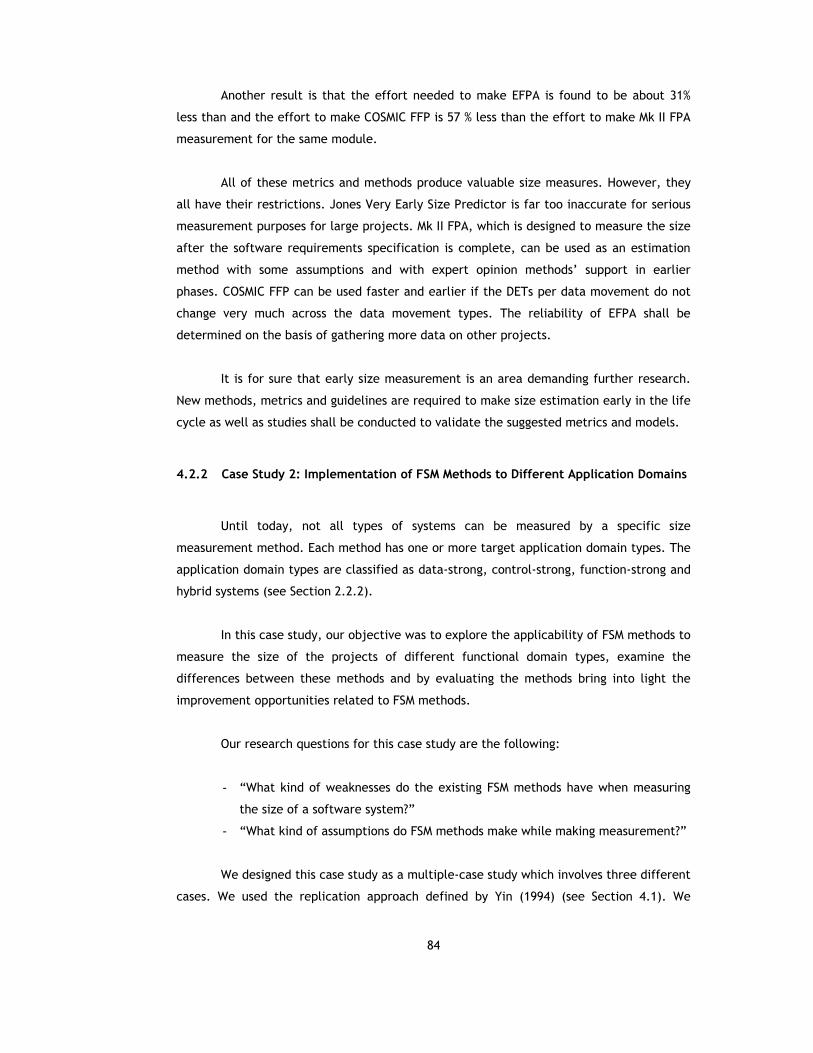
84

Another result is that the effort needed to make EFPA is found to be about 31%

less than and the effort to make COSMIC FFP is 57 % less than the effort to make Mk II FPA

measurement for the same module.

All of these metrics and methods produce valuable size measures. However, they

all have their restrictions. Jones Very Early Size Predictor is far too inaccurate for serious

measurement purposes for large projects. Mk II FPA, which is designed to measure the size

after the software requirements specification is complete, can be used as an estimation

method with some assumptions and with expert opinion methods’ support in earlier

phases. COSMIC FFP can be used faster and earlier if the DETs per data movement do not

change very much across the data movement types. The reliability of EFPA shall be

determined on the basis of gathering more data on other projects.

It is for sure that early size measurement is an area demanding further research.

New methods, metrics and guidelines are required to make size estimation early in the life

cycle as well as studies shall be conducted to validate the suggested metrics and models.

4.2.2 Case Study 2: Implementation of FSM Methods to Different Application Domains

Until today, not all types of systems can be measured by a specific size

measurement method. Each method has one or more target application domain types. The

application domain types are classified as data-strong, control-strong, function-strong and

hybrid systems (see Section 2.2.2).

In this case study, our objective was to explore the applicability of FSM methods to

measure the size of the projects of different functional domain types, examine the

differences between these methods and by evaluating the methods bring into light the

improvement opportunities related to FSM methods.

Our research questions for this case study are the following:

- “What kind of weaknesses do the existing FSM methods have when measuring

the size of a software system?”

- “What kind of assumptions do FSM methods make while making measurement?”

We designed this case study as a multiple-case study which involves three different

cases. We used the replication approach defined by Yin (1994) (see Section 4.1). We

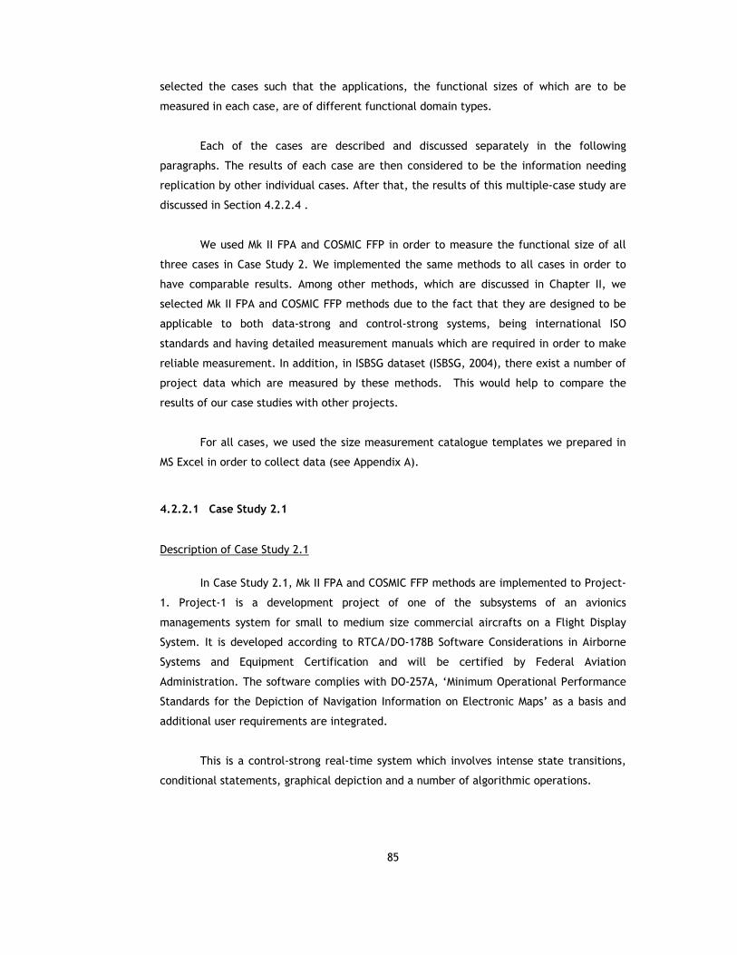
85

selected the cases such that the applications, the functional sizes of which are to be

measured in each case, are of different functional domain types.

Each of the cases are described and discussed separately in the following

paragraphs. The results of each case are then considered to be the information needing

replication by other individual cases. After that, the results of this multiple-case study are

discussed in Section 4.2.2.4 .

We used Mk II FPA and COSMIC FFP in order to measure the functional size of all

three cases in Case Study 2. We implemented the same methods to all cases in order to

have comparable results. Among other methods, which are discussed in Chapter II, we

selected Mk II FPA and COSMIC FFP methods due to the fact that they are designed to be

applicable to both data-strong and control-strong systems, being international ISO

standards and having detailed measurement manuals which are required in order to make

reliable measurement. In addition, in ISBSG dataset (ISBSG, 2004), there exist a number of

project data which are measured by these methods. This would help to compare the

results of our case studies with other projects.

For all cases, we used the size measurement catalogue templates we prepared in

MS Excel in order to collect data (see Appendix A).

4.2.2.1 Case Study 2.1

Description of Case Study 2.1

In Case Study 2.1, Mk II FPA and COSMIC FFP methods are implemented to Project-

1. Project-1 is a development project of one of the subsystems of an avionics

managements system for small to medium size commercial aircrafts on a Flight Display

System. It is developed according to RTCA/DO-178B Software Considerations in Airborne

Systems and Equipment Certification and will be certified by Federal Aviation

Administration. The software complies with DO-257A, ‘Minimum Operational Performance

Standards for the Depiction of Navigation Information on Electronic Maps’ as a basis and

additional user requirements are integrated.

This is a control-strong real-time system which involves intense state transitions,

conditional statements, graphical depiction and a number of algorithmic operations.

86

The software development organization is a SW-CMM Level 3 (Paulk et al., 1993)

company. The project was started in November 2003 and expected to be completed in

September 2005. The coding phase was completed and the testing phase has been

continuing. This case study was conducted in April 2005.

The project staff consisted of;

- 1 project manager: 13 years of experience; 6 years experience as a project

manager,

- 1 senior software engineer (development team leader): 7 years experience in

C, C++ software development for real-time systems, design of OO software with

UML,

- 6 software engineers (development team): 4 junior engineers less than 1 year

experience, 2 junior engineers experience between 2-3 years,

- 1 senior software test engineer (test team leader): 13 years experience, 5 years

experience as a test team leader on DO-178B verification projects,

- 2 junior software test engineer (test team): less than 1 year experience,

- 1 software quality engineer: 6 year experience as a software quality engineer,

4 years experience in DO-178B projects,

- 1 software configuration management specialist: 10 years experience in

software configuration management area.

The efforts of the project were collected on a daily basis in 0.25 hour intervals for

each work breakdown structure (WBS) task. The efforts utilized for the life cycle processes

of the project are given in Table 17.

The types of software products and programming language(s) used for the project

are:

- Software Requirements Analysis - Telelogic DOORS

- Software Design (Object Oriented) – Rhapsody

- Software Coding - Visual Studio C++

87

Table 17 Efforts Utilized for the Life Cycle Processes of Project-1

Software Development Life Cycle Phase Effort (person-hours) Development 18,003.12

Software Requirements Analysis 2,979.00 Software Design (Architectural-Detailed) 3,801.50 Software Coding & Unit Testing 5,960.12 Test Preparation (continuing) 5,104.50 Test Execution (continuing) 158.00

Management 2,316.25 Planning 855.75 Tracking & Oversight 794.75 Inter-group Coordination 665.75

Training 1,437.50 Supporting 2,351.00

Requirements Management 271.50 Software Quality Assurance activities (audits, reviews, inspections, walkthroughs) 1,120.00

Configuration Management 205.00 Customer Support 754.50

Total 24,107.87

Case Study Conduct and Data Collection

Implementation of the MkII FPA and COSMIC FFP Methods. For size measurement, we used

the Software Requirements Specification (SRS) document of Project-1, which involves 835

FURs. It is developed according to RTCA/DO-178B Software Considerations in Airborne

Systems and Equipment Certification and will be certified by Federal Aviation

Administration. Therefore, the abstraction level of FURs complies with this standard and is

very detailed. An example FUR might give an idea on the level of FURs:

IF (“Map Option” selected AND State 1 AND

((‘ActivePage’ is “X” AND ‘X_Place’ is “A”) OR

(‘ActivePage’ is “Y” AND ‘X_Place’ is “A”) OR

(‘ActivePage’ is “M” AND ‘X_Place’ is “A”) AND

(Data “ABC” valid)

THEN (State 2 AND Output_1 (attributes) AND Output_2 (attributes) AND Output_3

(attribute))

Two persons involved in the size measurement process. One of them is one of the

project managers of the project in the development organization. The other is the author

88

of this thesis study. Although both of them are experienced in using the methods, they are

not certified by UKSMA and COSMIC.

By Mk II FPA, the functional size of the project is measured as 5,160.16 Mk II FP

(see Table 18). Since Project-1 involves three subsystems, the measurement details are

given according to these subsystems. The effort utilized to make the measurement is 71.38

person-hours. The measurement catalogue is given in Appendix C.

Table 18 Case Study 2.1 Mk II FPA Size Measurement Details

Subsystem Number of

Logical Transactions

Number of

Input DETs

Number of

Output DETs

Number of Data Entity

Types Referenced

Functional Size

(Mk II FP)

A 443 661 2,344 2,037 4,374.24 B 33 112 160 198 435.24 C 45 51 156 169 350.68

Total 521 824 2,660 2,404 5,160.16

By applying COSMIC FFP, the functional size of the project is estimated as 4,036.0

Cfsu. The details are given in Table 19. The effort utilized to make COSMIC FFP

measurement is 56.50 person-hours. The measurement catalogue is given in Appendix C.

Table 19 Case Study 2.1 COSMIC FFP Size Measurement Details

Subsystem Number of Functional Processes

Number of

Entries

Number of

Exits

Number of

Reads

Number of

Writes

Functional Size (Cfsu)

A 443 521 729 1,946 309 3,505.0 B 33 49 32 198 0 279.0 C 45 45 40 159 8 252.0

Total 521 615 801 2,303 317 4,036.0

In Table 20, the productivity rates (Code & Unit Test Effort / Functional size) for

the subsystems of Case Study 2.1 are given.

89

Table 20 The Productivity Rates (Code & Unit Test Effort / Functional Size) of the Subsystems of Case Study 2.1

Subsystem Code & Unit Test Effort

(man- hours)

Functional Size

(Mk II FP)

Functional Size

(Cfsu)

Productivity (man-hours/

Mk II FP)

Productivity (man-hours/

Cfsu) A 5,410.50 4,374.24 3,505.00 1.24 1.54

B 329.77 435.24 279.00 0.76 1.18

C 219.85 350.68 252.00 0.63 0.87

Total 5,960.12 5,160.16 4,036.00 1.16 1.48

In Table 21, the productivity rates (Development Effort / Functional Size) of Case

Study 2.1 are given. Since the development efforts of each subsystem were not collected

by the project team, we give these values with respect to the whole project.

In Table 22, the productivity rates (Code & Unit Test Effort / SLOC) for the

subsystems of Case Study 2.1 are given.

Table 21 The Productivity Rates (Development Effort/Functional Size) of Case Study2.1

Development Effort

(man- hours)

Functional Size (Mk II FP)

Functional Size (Cfsu)

Productivity (man-hours/

Mk II FP)

Productivity (man-hours/

Cfsu) 18,003.12 5,160.16 4,036.00 3.49 4.46

Table 22 The Productivity Rates (Code & Unit Test Effort / SLOC) of Case Study 2.1

Subsystem Code & Unit Test Effort

(man- hours)

SLOC (Physical,Un-commented)

SLOC (Logical,Un-commented)

Productivity (man-hours/

Physical SLOC)

Productivity (man-hours/

Logical SLOC)

A 5,410.50 20,196 12,143 0.27 0.45

B 329.77 6,115 3,449 0.05 0.10

C 219.85 6,698 3,914 0.03 0.06

Total 5,960.12 33,009 19,506 0.18 0.31

90

Table 23 shows the productivity rates (Development Effort / SLOC) of Case Study

2.1. The SLOC values for all three subsystems are obtained by using Understand for C++

which is a source code analyzer. Both logical and physical un-commented SLOC values are

measured.

Table 23 The Productivity (Development Effort / SLOC) Values of Case Study 2.1

Development Effort

(man- hours)

SLOC (Physical,

Un-commented)

SLOC (Logical,

Un-commented)

Productivity (man-hours/

Physical SLOC)

Productivity (man-hours/

Logical SLOC)

18,003.12 33,009 19,506 0.55 0.92

In Table 24, the ratios of Functional Size to Un-commented Logical SLOC values for

each subsystem of Case Study 2.1 are given.

Table 24 The Ratio of Functional Size (Mk II FP & Cfsu) to SLOC Values of Case Study2.1

Subsystem Functional Size (Mk II FP)

Functional Size (Cfsu)

SLOC (Logical)

SLOC / Mk II FP

SLOC / Cfsu

A 4,374.24 3,505.0 12,143 2.78 3.46

B 435.24 279.0 3,449 7.92 12.36

C 350.68 252.0 3,914 11.16 15.53

Total 5,160.16 4,036.0 19,506 3.78 4.83

4.2.2.2 Case Study 2.2

Description of Case Study 2.2

In Case Study 2.2, Mk II FPA and COSMIC FFP methods are implemented to Project-

2. Project-2 is a Collision Avoidance Subsystem (CAS) which provides the collision

avoidance functionality for the TCAS (Traffic Collision Avoidance System) system. It is

91

developed according to RTCA/DO-178B Software Considerations in Airborne Systems and

Equipment Certification and will be certified by Federal Aviation Administration. CAS

functionality is specified in detail in the CAS Requirements Specification (DO-185A, Vol. 2).

In this study, we measured the size of CAS-Own Aircraft Algorithm. Own Aircraft

function determines the TCAS operational mode, effective sensitivity level and other

operation parameters used by the collision avoidance logic. This function also is

responsible for tracking of own aircraft altitude, determination of the Resolution Advisory

(RA) outputs, transmission of Resolution Coordination interrogations, RA Broadcast

messages and update of own collision avoidance capabilities to the Mode S transponder.

This case is a hybrid real-time system which involves intense state transitions, algorithmic

calculations and conditional statements.

The software development organization is the same company as Project-1 in Case

Study 2.1, which is a SW-CMM Level 3 (Paulk et al., 1993) company. The project was

started in September 2004 and expected to be completed in July 2005. This case study was

conducted in May 2005.

The project staff consisted of;

- 1 project manager: 11 years experience, 4 years experience as a project

manager,

- 1 senior software engineer (development team leader): 5 years experience in

C, C++ software development for real-time systems,

- 3 software engineers (development team): junior engineers less than 1 year

experience,

- 1 software test engineer (test team leader): 5 years experience as a test

engineer on DO-178B verification projects,

- 1 junior software test engineer (test team): junior engineer less than 1 year

experience,

- 1 software quality engineer: 2 year experience as a software quality engineer,

first experience in a DO-178B project,

- 1 software configuration management specialist: 6 years experience in software

configuration management area.

The efforts were collected on a daily basis in 0.25 hour intervals for each work

breakdown structure (WBS) task. The efforts utilized for the life cycle processes of the

project are given in Table 25.

92

Table 25 Efforts Utilized for the Life Cycle Processes of Case Study 2.2

Software Development Life Cycle Phase Effort (person-hours) Development 2,199.75

Software Requirements Analysis 138.50 Software Design (Architectural-Detailed) 336.50 Software Coding & Unit Testing 1,676.25 Test Preparation(continuing) 48.50

Management 1,418.00 Planning 280.25 Tracking & Oversight 958.25 Inter-group Coordination 179.50

Training 179.50 Supporting 1,986.00

Software Quality Assurance activities (audits, reviews, inspections, walkthroughs) 1,676.75

Configuration Management 309.25 Total 5,783.25

CAS functionality is specified in detail in the CAS Requirements Specification (DO-

185A, volume 2). Therefore, since the software functional requirements were written

according to this standard, the utilized effort for the Software Requirements Analysis

phase is low.

The types of software products and programming language(s) used during

development:

- Software Requirements Analysis - Telelogic Doors

- Software Design (Structural) - Rhapsody

- Software Coding - Visual Studio C

Case Study Conduct and Data Collection

Implementation of the MkII FPA and COSMIC FFP Methods. In Case Study 2.2, we used the

SRS document of Project-2 for size measurement. The number of FURs is 158. Since the

system will be certified by Federal Aviation Administration, it is developed according to

RTCA/DO-178B as Case Study 2.1. Therefore, the level of FURs is very similar to Case Study

2.1.

Two persons involved in the size measurement process. One of the persons works

for the development organization of the project. Although he is not involved in the

93

development process of this project, he has the domain knowledge about these kinds of

applications. The other one is the author of this thesis study. Although both of them are

experienced in using the methods, they are not certified by UKSMA and COSMIC.

By Mk II FPA, the functional size of the project is measured as 1,179.62 Mk II FP.

The details of the size measurement are given in Table 26. The effort utilized is 54.50

person-hours. The measurement catalogue is given in Appendix C.

Table 26 Case Study 2.2 Mk II FPA Size Measurement Details

Number of Logical

Transactions

Number of Input DETs

Number of Output DETs

Number of Data Entity Types Referenced

Functional Size (Mk II FP)

99 283 126 592 1,179.62

By applying COSMIC FFP, the functional size of the project is measured as 945 Cfsu

(see Table 27). The effort utilized to make COSMIC FFP measurement is 12.50 person-

hours. The measurement catalogue is given in Appendix C

Table 27 Case Study 2.2 COSMIC FFP Size Measurement Details

Number of Functional Processes

Number of Entries

Number of Exits

Number of Reads

Number of Writes

Functional Size (Cfsu)

99 206 51 588 100 945

In Table 28, the productivity rates (Code & Unit Test Effort / Functional size) of

Case Study 2.2 are given.

94

Table 28 The Productivity Rates (Code & Unit Test Effort/Funct. Size) of Case Study 2.2

Code & Unit Test Effort

(man- hours)

Functional Size

(Mk II FP)

Functional Size

(Cfsu)

Productivity (man-hours/

Mk II FP)

Productivity (man-hours/

Cfsu) 1,676.25 1,179.62 945.00 1.42 1.77

In Table 29, the productivity rates (Development Effort / Functional size) of Case

Study 2.2 are given.

Table 29 The Productivity Rates (Development Effort/Functional Size) of Case Study2.2

Development Effort (man- hours)

Functional Size

(Mk II FP)

Functional Size

(Cfsu)

Productivity (man-hours/

Mk II FP)

Productivity (man-hours/

Cfsu) 2,199.75 1,179.62 945.0 1.86 2.33

In Table 30, the productivity rates (Code & Unit Test Effort / SLOC) for Case Study

2.2 are given.

Table 30 The Productivity (Code & Unit Test Effort / SLOC) Values of Case Study 2.2

Code & Unit Test Effort

(man- hours)

SLOC (Physical, Un-commented)

SLOC (Logical, Un-commented)

Productivity (man-hours/

Physical SLOC)

Productivity (man-hours/ Logical SLOC)

1,676.25 937 289 1.79 5.80

Table 31 shows the productivity rates (Development Effort / SLOC) of Case Study

2.2. The SLOC values for Case Study 2.2 are obtained by using Understand for C++ which is

a source code analyzer. By this tool, both the logical and physical un-commented SLOC

values are measured.

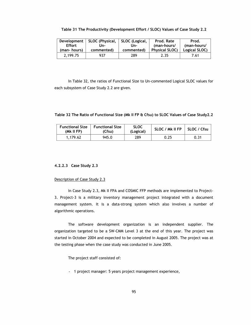
95

Table 31 The Productivity (Development Effort / SLOC) Values of Case Study 2.2

Development Effort

(man- hours)

SLOC (Physical, Un-

commented)

SLOC (Logical, Un-

commented)

Prod. Rate (man-hours/

Physical SLOC)

Prod. (man-hours/ Logical SLOC)

2,199.75 937 289 2.35 7.61

In Table 32, the ratios of Functional Size to Un-commented Logical SLOC values for

each subsystem of Case Study 2.2 are given.

Table 32 The Ratio of Functional Size (Mk II FP & Cfsu) to SLOC Values of Case Study2.2

Functional Size (Mk II FP)

Functional Size (Cfsu)

SLOC (Logical) SLOC / Mk II FP SLOC / Cfsu

1,179.62 945.0 289 0.25 0.31

4.2.2.3 Case Study 2.3

Description of Case Study 2.3

In Case Study 2.3, Mk II FPA and COSMIC FFP methods are implemented to Project-

3. Project-3 is a military inventory management project integrated with a document

management system. It is a data-strong system which also involves a number of

algorithmic operations.

The software development organization is an independent supplier. The

organization targeted to be a SW-CMM Level 3 at the end of this year. The project was

started in October 2004 and expected to be completed in August 2005. The project was at

the testing phase when the case study was conducted in June 2005.

The project staff consisted of:

- 1 project manager: 5 years project management experience,

96

- 1 senior software engineer (development team – full time): 5 years software

development experience, expert in object oriented analysis, design with UML,

development with Java, database design, familiar with Internal Development

Framework, good at Oracle,

- 1 software engineer (development team – full time): 3 years software

development experience; expert in object oriented analysis, design with UML,

development with Java, database design, familiar with Internal Development

Framework, good at Oracle,

- 1 software engineer (development team - part time): 2 year software

development experience; expert in object oriented analysis, design with UML,

development with Java, familiar with Internal Development Framework, good

at Oracle,

- 1 software engineer (development team - part time): familiar with Java,

Internal Development Framework and Oracle,

- 1 software engineer (test team – part time).

The efforts utilized for the development and management activities of the project

are given in Table 33. Support and training activities are planned but at the time of the

conduct of this case study, these were not completed. Therefore, the efforts for these

activities are not given.

Table 33 Efforts Utilized for the Life Cycle Processes of Case Study 2.3

Software Development Life Cycle Phase Effort (person-hours) Development 3,908.00

Software Requirements Analysis 911.00 Software Design (Architectural-Detailed) 698.00 Software Coding & Unit Testing 2,151.00 Test Preparation(continuing) 148.00

Management 225.00 Total 4,133.00

The types of software products and programming language(s) used for the project

are:

- Analysis and Design tool; Rational Rose

- Development: IBM WebSphere Application Developer

97

- Tomcat application server

- Oracle 9i database management system

- Internal Development Framework

Case Study Conduct and Data Collection

Implementation of the Mk II FPA and COSMIC FFP Methods. In Case Study 2.3, we used the

SRS document of Project-3, which involves 127 Use Cases. The company uses an SRS

standard developed by the company itself. The levels of the FURs are detailed. Most of the

Use Cases correspond to a Logical Transaction (or Functional Process) of the FSM methods.

Two persons made the size measurement. One of the persons works for the

development organization and involved in this project. The other one is the author of this

thesis study. Although both of them are experienced in using the methods, they are not

certified by UKSMA and COSMIC.

By Mk II FPA, the functional size of the project is measured as 1,338.00 Mk II FP.

The details of the size measurement are given in Table 34. The effort utilized is 23.33

person-hours. The measurement catalogue is given in Appendix C.

Table 34 Case Study 2.3 Mk II FPA Size Measurement Details

Number of Logical

Transactions

Number of Input DETs

Number of Output DETs

Number of Data Entity Types Referenced

Functional Size (Mk II FP)

127 560 1,707 343 1,338.00

By applying COSMIC FFP, the functional size of the project is measured as 1,020.0

Cfsu (see Table 35). The effort utilized to make COSMIC FFP measurement is 12.58 person-

hours. The measurement catalogue is given in Appendix C.

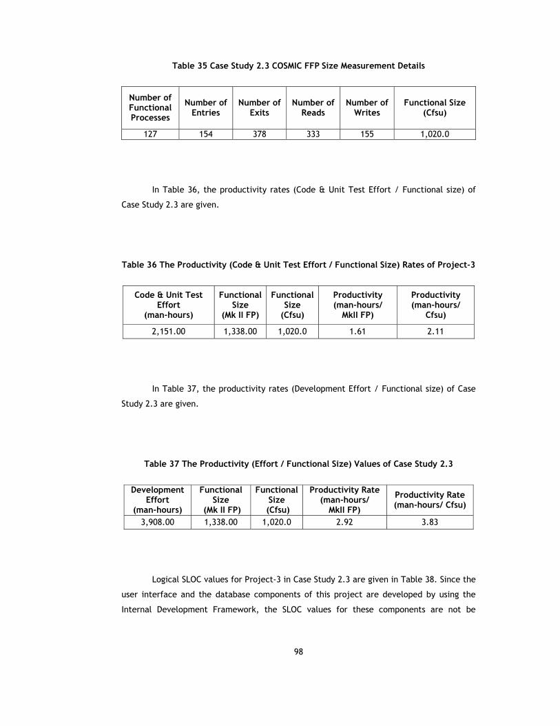
98

Table 35 Case Study 2.3 COSMIC FFP Size Measurement Details

Number of Functional Processes

Number of Entries

Number of Exits

Number of Reads

Number of Writes

Functional Size (Cfsu)

127 154 378 333 155 1,020.0

In Table 36, the productivity rates (Code & Unit Test Effort / Functional size) of

Case Study 2.3 are given.

Table 36 The Productivity (Code & Unit Test Effort / Functional Size) Rates of Project-3

Code & Unit Test Effort

(man-hours)

Functional Size

(Mk II FP)

Functional Size

(Cfsu)

Productivity (man-hours/

MkII FP)

Productivity (man-hours/

Cfsu)

2,151.00 1,338.00 1,020.0 1.61 2.11

In Table 37, the productivity rates (Development Effort / Functional size) of Case

Study 2.3 are given.

Table 37 The Productivity (Effort / Functional Size) Values of Case Study 2.3

Development Effort

(man-hours)

Functional Size

(Mk II FP)

Functional Size

(Cfsu)

Productivity Rate (man-hours/

MkII FP)

Productivity Rate (man-hours/ Cfsu)

3,908.00 1,338.00 1,020.0 2.92 3.83

Logical SLOC values for Project-3 in Case Study 2.3 are given in Table 38. Since the

user interface and the database components of this project are developed by using the

Internal Development Framework, the SLOC values for these components are not be

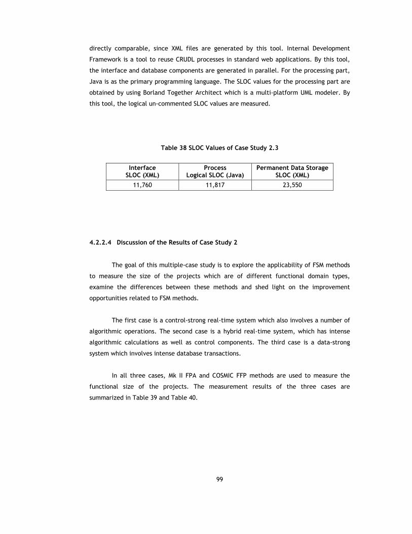
99

directly comparable, since XML files are generated by this tool. Internal Development

Framework is a tool to reuse CRUDL processes in standard web applications. By this tool,

the interface and database components are generated in parallel. For the processing part,

Java is as the primary programming language. The SLOC values for the processing part are

obtained by using Borland Together Architect which is a multi-platform UML modeler. By

this tool, the logical un-commented SLOC values are measured.

Table 38 SLOC Values of Case Study 2.3

Interface SLOC (XML)

Process Logical SLOC (Java)

Permanent Data Storage SLOC (XML)

11,760 11,817 23,550

4.2.2.4 Discussion of the Results of Case Study 2

The goal of this multiple-case study is to explore the applicability of FSM methods

to measure the size of the projects which are of different functional domain types,

examine the differences between these methods and shed light on the improvement

opportunities related to FSM methods.

The first case is a control-strong real-time system which also involves a number of

algorithmic operations. The second case is a hybrid real-time system, which has intense

algorithmic calculations as well as control components. The third case is a data-strong

system which involves intense database transactions.

In all three cases, Mk II FPA and COSMIC FFP methods are used to measure the

functional size of the projects. The measurement results of the three cases are

summarized in Table 39 and Table 40.

100

Table 39 Case Study-2 Mk II FPA Size Measurement Details

Case Study

Project Name Subsystem Number

of FURs

Number of Logical

Transactions

Number of Input DETs

Number of Output DETs

Number of Data Entity Types Referenced

Functional Size

(Mk II FP) A 758 443 661 2,344 2,037 4,374.24 B 37 33 112 160 198 435.24 C 40 45 51 156 169 350.68

2.1 Project-1

Total 835 521 824 2,660 2,404 5,160.16 2.2 Project-2 158 99 283 126 592 1,179.62 2.3 Project-3 127 127 560 1,707 343 1,338.00

Table 39 Case Study-2 Mk II FPA

Size Measurem

ent Details

101

Table 40 Case Study-2 COSMIC FFP Size Measurement Details

Case Study

Project Name Subsystem Number

of FURs

Number of Functional Processes

Number of Entries

Number of Exits

Number of Reads

Number of Writes

Functional Size (Cfsu)

A 758 443 521 729 1,946 309 3,505.00 B 37 33 49 32 198 0 279.00 C 40 45 45 40 159 8 252.00

2.1 Project-1

Total 835 521 615 801 2,303 317 4,036.00 2.2 Project-2 158 99 206 51 588 100 945.00 2.3 Project-3 127 127 154 378 333 155 1,020.00

Table 40 Case Study-2 COSM

IC FFP Size Measurem

ent Details

102

We could not compare the functional sizes obtained by Mk II FPA and COSMIC FFP

since these methods use different metrics. In order to compare Mk II FPA and COSMIC FFP

measures, we need to convert these values to each other. However, there exists no such

conversion formula in the literature yet. The differences between the rules and

assumptions of Mk II FPA and COSMIC FFP on measuring the BFCs make it difficult to define

a conversion formula. Therefore, we compared the results of both methods according to

the base counts in order to depict what kind of factors might give rise to obtain different

functional sizes.

By MkII FPA, the number of references to Data Entity Types is 2,404, 592, and 343

in Case Study 2.1, Case Study 2.2, and Case Study 2.3, respectively. By COSMIC FFP, the

total number of data groups that are read or written is 2,620 in Case Study 2.1, 688 in

Case Study 2.2 and 488 in Case Study 2.3.

In Mk II FPA, the size of the processing component of a LT is defined to be

proportional to the number of referenced Data Entity Types. A Data Entity Reference in Mk

II FPA is generally equivalent to a Read or Write in COSMIC FFP. Therefore, the sizes of the

processing component are roughly equivalent on both scales (ISO/IEC 19761, 2003).

However, one of the distinctions of these two methods is the assumptions of the methods

when measuring the size of the processing component. Mk II FPA assumes that each LT

must have at least 1 input DET, must make 1 reference to a Data Entity Type and must

have 1 output DET as a minimum. On the other hand, COSMIC FFP principles say that “A

Functional Process comprises at least two data movements, an entry plus either an exit or

a write”.

Therefore, in Mk II FPA, for a specific LT, we should count at least 1 entity

reference for the processing component in case a Data Entity Type is not accessed. In

COSMIC FFP, we do not count anything related to the processing components if there is no

Read or Write to a data group.

In all three cases, the numbers of processing components are higher in COSMIC FFP

than in Mk II FPA. This means that there exist Data Entity Types which are both read and

written in a LT (or a Functional Process). These are counted only once in Mk II FPA

whereas they are counted separately as Entries and Exits in COSMIC FFP.

By Mk II FPA, the functional sizes of the processing component of Case Study 2.1,

Case Study 2.2, and Case Study 2.3 are 3,990.64, 982.72, 569.38 Mk II FP, respectively. By

COSMIC FFP, the functional sizes of the processing component of Case Study 2.1 are 2,620

103

Cfsu, Case Study 2.2 is 688 Cfsu and Case Study 2.3 is 488 Cfsu. Although we expect higher

functional size by COSMIC FFP, the weight factor used in Mk II FPA changes the result. That

is, when calculating the functional size of the processing component, we multiply the

number of references by 1.66 in Mk II FPA whereas there is no weight factor in COSMIC

FFP.

As a result, we may find varying correlation values between the number of

references to the processing entities and the total number of Reads and Writes for

different kinds of software which makes it difficult to find a conversion formula.

The second distinction between Mk II FPA and COSMIC FFP causes the functional

sizes of input and output components obtained by these two methods to be different. This

is the level of granularity in each method’s size measurement process. COSMIC FFP method

estimates functional size at a higher level of granularity than Mk II FPA. The COSMIC FFP

unit of measurement, 1 Cfsu, has been fixed at the level of one data movement. On the

other hand, in Mk II FPA method, the size of the input and output components of a LT is

defined to be proportional to the number of DETs in the input and output components. The

users of COSMIC FFP are warned to be careful when comparing the sizes of two different

pieces of software where the average number of DETs per data movement differs sharply

across the two pieces of software (ISO/IEC 19761, 2003).

In Case Study 2.1, the number of input DETs is 824, the number of output DETs is

2,660 in Mk II FPA measurement and the functional size of input and output components

are found to be 477.92 Mk II FP and 691.60 Mk II FP, respectively. By implementing COSMIC

FFP, the number of Entries and the number of Exits are found to be 615 and 801,

respectively. The functional size of Entries is 615 Cfsu and Exits is 801 Cfsu.

In Case Study 2.2, by implementing Mk II FPA, the number of input DETs is found to

be 283 and the number of output DETs as 126. The functional size of input and output

components are 164.14 Mk II FP and 32.76 Mk II FP, respectively. In COSMIC FFP

measurement, the number of Entries is 206 and the number of Exits is 51. The functional

sizes of Entries and Exits are 206 Cfsu and 51 Cfsu, respectively.

In Case Study 2.3, the number of input DETs is 560, the number of output DETs is

1,707 in Mk II FPA measurement and the functional size of input and output components

are 324.80 Mk II FP and 443.82 Mk II FP, respectively. By COSMIC FFP, the number of

Entries is 154 and the number of Exits is 378. The functional sizes of Entries and Exits are

calculated as 154 Cfsu and 378 Cfsu, respectively.

104

The third distinction between Mk II FPA and COSMIC FFP is related to the

relationship between the functional sizes of different BFC Types and constituent parts of

BFC Types. Mk II FPA makes use of weight factors which are calibrated to industry-average

relative effort to develop each component. This enables these three kinds of functionality

to be combined into a single value for a functional size. On the other hand, COSMIC FFP

assumes that the average number of DETs per data movement does not vary much across

the four BFC Types, i.e. Entry, Exit, Read, Write. Thus, the contribution of each to

functional size is assumed to be the same.

The distinctions of MkII FPA and COSMIC FFP discussed above resulted in higher

sizes by Mk II FPA than by COSMIC FFP with a difference of 22 % in Case Study 2.1, 20 % in

Case Study 2.2, and 24 % in Case Study 2.3. Therefore, the practitioners should consider

their variance when making effort estimation from functional size figures of different FSM

methods.

One of the issues of the measurement process of Case Study 2.1 and Case Study

2.2 by both methods was identifying the elementary components of FURs, which are LTs in

Mk II FPA and Functional Processes in COSMIC FFP. Generally, a FUR consists of one or

more LTs or Functional Process(es). In the measurement manual of COSMIC FFP, it is

stated that “A Functional Process is derived from at least one identifiable FUR” (ISO/IEC

19761, 2003). In order to identify LTs or Functional Processes, FURs are decomposed into

their elementary components. However, in our case, we needed to gather and group two

or more FURs in order to form one LT or one Functional Process.

In Case Study 2.1 and Case Study 2.2, the total number of FURs is 835 and 158

whereas the total number of LTs (or FPs) is 521 and 99, respectively. This is due to the

fact that the level of FURs in the SRS document is very detailed, i.e. functional

transactions are specified and the related requirements which would form one LT (or FPs)

were organized such that each is specified in different parts of the document. As a result

one quarter of the total effort on measurement was utilized for this purpose in Case Study

2.1.

In the SRS document of Case Study 2.2, the FURs are organized such that the

functionality is specified with respect to a standard (DO-185A, volume 2). The algorithmic

operations (functions and macros) are specified in separate sections and the FURs give

reference to the macros and functions they make use of. In addition, each macro and

function gives reference to others as well. Therefore, we had to trace these paths in order

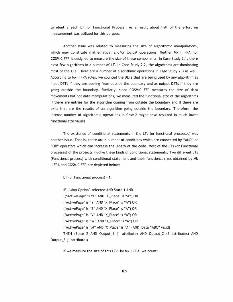
105

to identify each LT (or Functional Process). As a result about half of the effort on

measurement was utilized for this purpose.

Another issue was related to measuring the size of algorithmic manipulations,

which may constitute mathematical and/or logical operations. Neither Mk II FPA nor

COSMIC FFP is designed to measure the size of these components. In Case Study 2.1, there

exist few algorithms in a number of LT. In Case Study 2.2, the algorithms are dominating

most of the LTs. There are a number of algorithmic operations in Case Study 2.3 as well.

According to Mk II FPA rules, we counted the DETs that are being used by any algorithm as

input DETs if they are coming from outside the boundary and as output DETs if they are

going outside the boundary. Similarly, since COSMIC FFP measures the size of data

movements but not data manipulations, we measured the functional size of the algorithms

if there are entries for the algorithm coming from outside the boundary and if there are

exits that are the results of an algorithm going outside the boundary. Therefore, the

intense number of algorithmic operations in Case-2 might have resulted in much lower

functional size values.

The existence of conditional statements in the LTs (or functional processes) was

another issue. That is, there are a number of conditions which are connected by “AND” or

“OR” operators which can increase the length of the code. Most of the LTs (or Functional

processes) of the projects involve these kinds of conditional statements. Two different LTs

(Functional process) with conditional statement and their functional sizes obtained by Mk

II FPA and COSMIC FFP are depicted below:

LT (or Functional process) - 1:

IF (“Map Option” selected AND State 1 AND

((‘ActivePage’ is “X” AND ‘X_Place’ is “A”) OR

(‘ActivePage’ is “Y” AND ‘X_Place’ is “A”) OR

(‘ActivePage’ is “Z” AND ‘X_Place’ is “A”) OR

(‘ActivePage’ is “V” AND ‘X_Place’ is “A”) OR

(‘ActivePage’ is “W” AND ‘X_Place’ is “A”) OR

(‘ActivePage’ is “M” AND ‘X_Place’ is “A”) AND Data “ABC” valid)

THEN (State 2 AND Output_1 (1 attribute) AND Output_2 (2 attributes) AND

Output_3 (1 attribute))

If we measure the size of this LT-1 by Mk II FPA, we count:

106

- 1 DET for the input component (1 DET for “Map Option”)

- 4 DETs for the output (1 DET for Output_1, 2 DETs for Output_2, 1 DET for

Output_3)

- 4 references to Data Entity Types (value of ‘ActivePage’ is read from Entity-1,

value of ‘X_Place’ is read from Entity-2, the value of data “ABC” is read from

Entity – 3, State-1 is read from Entity -4 and State 2 is written to Entity - 4),

The size of this LT is 8.26 Mk II FP.

If we measure the size of this Functional Process by COSMIC FFP, we count:

- 1 Entry (“Map Option”),

- 3 Exits (Output_ 1, Output_ 2, Output_ 3)

- 4 Reads (value of ‘ActivePage’ is read from Entity-1, value of ‘X_Place’ is read

from Entity-2, the value of data “ABC” is read from Entity – 3, State-1 is read

from Entity -4)

- 1 Write (State 2 is written to Entity – 4)

The size of this Functional Process is 9 Cfsu.

LT (or Functional process) - 2:

IF (“Map Option” selected AND State 1 AND

((‘ActivePage’ is “X” AND ‘X_Place’ is “A”) AND Data “ABC” valid)

THEN (State 2 AND Output_1 (1 attribute) AND Output_2 (2 attributes) AND

Output_3 (1 attribute))

If we measure the size of this LT (or Functional Process)-2 by Mk II FPA and COSMIC

FFP, the results would be the same as LT (or Functional Process)-1 in spite of the fact that

the length of the codes of these two LTs would be different.

Table 41 summarizes the efforts utilized for functional size measurement in Case

Study 2.

In Case Study 2.1, the effort utilized to make the measurement by Mk II FPA is

71.38 person-hours whereas it took 56.50 person-hours to make COSMIC FFP measurement.

In Case Study 2.2; the effort utilized for Mk II FPA measurement is 54.50 person-hours and

it is 12.50 person-hours for COSMIC FFP measurement. In Case Study 2.3, the effort

107

utilized to make the measurement by Mk II FPA is 23.33 person-hours whereas it took 12.58

person-hours to make COSMIC FFP measurement.

Table 41 The Efforts Utilized for Functional Size Measurement in Case Study 2

Case Study No Effort Utilized By Mk II FPA (person-hours)

Effort Utilized by COSMIC FFP (person-hours)

Case Study 2.1 71.38 56.50 Case Study 2.2 54.50 12.50 Case Study 2.3 23.33 12.58

Although it seems that we utilized greater effort for Mk II FPA measurement in all

of the cases, we can not conclude that COSMIC FFP requires less effort to count

functionality of the same product. We measured the size of the projects by implementing

Mk II FPA first. Therefore, we did not utilize extra effort to identify Functional Processes

in COSMIC FFP since we had already identified LTs in Mk II FPA.

From the results of Case Study 2, we concluded that both methods can be used for

measuring the size of real-time systems, but with some restrictions when algorithmic

components and conditional statements exist. Another result is that COSMIC FFP can be

applied earlier in the development life cycle than Mk II FPA, since COSMIC FFP does not

need the number of DETs in the input and output components. However, this requires that

the average number of DETs does not vary across the BFC Types.

4.2.3 Case Study 3: Implementation of ARCHI-DIM FSM

In this case-study our aim is to explore the applicability of the new FSM method we

introduced in Chapter 3: ARCHI-DIM FSM to software systems which are of different

functional domain types. We applied ARCHI-DIM FSM to the same software systems as in

Case Study 2 in order to evaluate the improvement suggestions of this new method.

According to the findings of this case study, some gradual improvements have been made.

In addition, a number of improvement suggestions for ARCHI-DIM FSM are discussed in the

future research section (see Section 6.2).

108

Our research questions for this case study are the following:

- “Does ARCHI-DIM FSM bring advantages over the existing FSM methods by its

improvement suggestions?”

- “What kind of new improvement points can be identified?”

We designed this case study as a multiple-case study which involves three different

cases. Each individual case is described and discussed separately in the following sections.

After that, the results of this multiple-case study are discussed in Section 4.2.3.4.

4.2.3.1 Case Study 3.1

Description of Case Study 3.1

Since the project to which ARCHI-DIM FSM was implemented is Project-1 as in the

first case of Case Study 2, we do not repeat the description of the project in this section

(see Section 4.2.2.1 for the description of Project-1).

Case Study Conduct and Data Collection

Implementation of ARCHI-DIM FSM Method. For size measurement, we used the Software

Requirements Specification (SRS) document of Project-1, which involves 835 FURs. Two

persons were involved in the size measurement process. One of them is one of the project

managers of the project in the development organization. The other one is the author of

this thesis study.

The functional size of the case is measured by ARCHI-DIM FSM after the COSMIC

FFP and Mk II FPA based measurements are completed.

The details of the measurement are given in Table 42. The measurement catalogue

is given in Appendix C. The effort utilized to make the measurement is 99.50 person-hours.

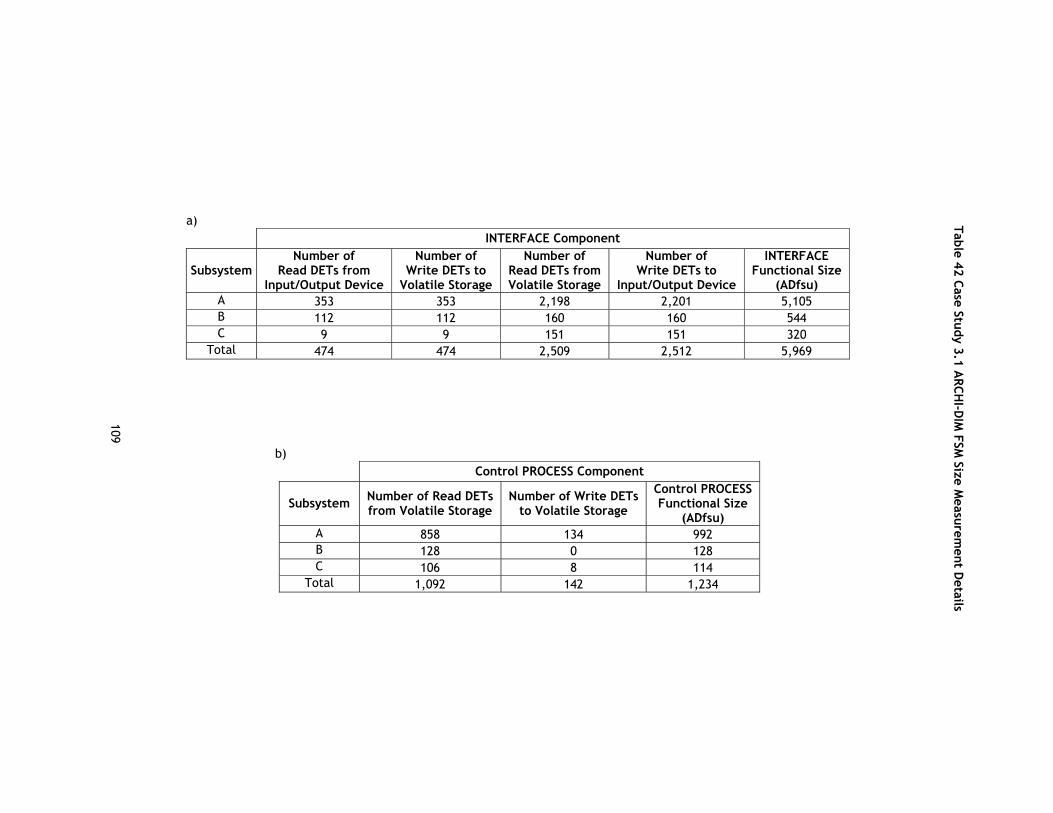
109

Table 42 Case Study 3.1 ARCHI-DIM FSM Size Measurement Details

a) INTERFACE Component

Subsystem Number of

Read DETs from Input/Output Device

Number of Write DETs to

Volatile Storage

Number of Read DETs from Volatile Storage

Number of Write DETs to

Input/Output Device

INTERFACE Functional Size

(ADfsu) A 353 353 2,198 2,201 5,105 B 112 112 160 160 544 C 9 9 151 151 320

Total 474 474 2,509 2,512 5,969

b) Control PROCESS Component

Subsystem Number of Read DETs from Volatile Storage

Number of Write DETs to Volatile Storage

Control PROCESS Functional Size

(ADfsu) A 858 134 992 B 128 0 128 C 106 8 114

Total 1,092 142 1,234

Table 42 Case Study 3.1 ARCH

I-DIM

FSM Size M

easurement D

etails

110

Table 42 Case Study 3.1 ARCHI-DIM FSM Size Measurement Details (cont.)

c) Algorithmic/Data Manipulation PROCESS Component

Subsystem Number of

Read DETs from Volatile Storage

Number of Write DETs to

Volatile Storage

Algorithmic / Data Manipulation PROCESS Functional Size

(ADfsu) A 687 941 1,628 B 216 120 336 C 99 80 179

Total 1,002 1,141 2,143 d)

PERMANENT STORAGE Data Access / Storage Component

Subsystem Number of

Read DETs from Permanent Storage

Number of Write DETs to

Permanent Storage

Number of Read DETs from Volatile Storage

Number o Write DETs to

Volatile Storage

PERMANENT STORAGE Data Access/Storage

Functional Size (ADfsu)

A 2,983 334 734 3,007 7,058 B 200 0 0 200 400 C 150 0 32 150 332

Total 3,333 334 766 3,357 7,790

Table 42 Case Study 3.1 ARCH

I-DIM

FSM Size M

easurement D

etails (cont.)

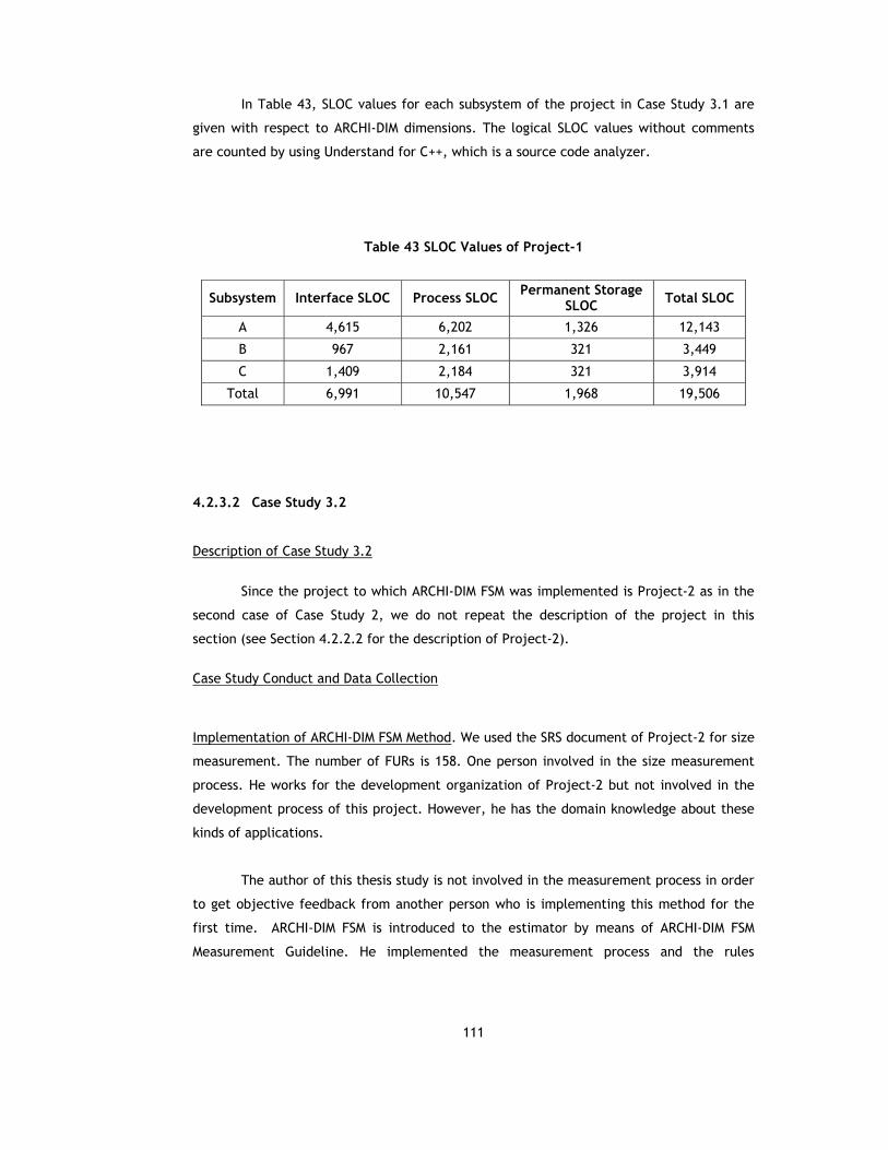
111

In Table 43, SLOC values for each subsystem of the project in Case Study 3.1 are

given with respect to ARCHI-DIM dimensions. The logical SLOC values without comments

are counted by using Understand for C++, which is a source code analyzer.

Table 43 SLOC Values of Project-1

Subsystem Interface SLOC Process SLOC Permanent Storage SLOC Total SLOC

A 4,615 6,202 1,326 12,143

B 967 2,161 321 3,449

C 1,409 2,184 321 3,914

Total 6,991 10,547 1,968 19,506

4.2.3.2 Case Study 3.2

Description of Case Study 3.2

Since the project to which ARCHI-DIM FSM was implemented is Project-2 as in the

second case of Case Study 2, we do not repeat the description of the project in this

section (see Section 4.2.2.2 for the description of Project-2).

Case Study Conduct and Data Collection

Implementation of ARCHI-DIM FSM Method. We used the SRS document of Project-2 for size

measurement. The number of FURs is 158. One person involved in the size measurement

process. He works for the development organization of Project-2 but not involved in the

development process of this project. However, he has the domain knowledge about these

kinds of applications.

The author of this thesis study is not involved in the measurement process in order

to get objective feedback from another person who is implementing this method for the

first time. ARCHI-DIM FSM is introduced to the estimator by means of ARCHI-DIM FSM

Measurement Guideline. He implemented the measurement process and the rules

112

discussed in the manual. The feedback provided by the estimator during an interview

session, are given in Section 4.2.3.4.

The functional size of the Project-2 was measured by ARCHI-DIM FSM after the

COSMIC FFP and Mk II FPA based measurements are completed.

The details of the measurement are given in Table 44. The measurement catalogue

is given in Appendix C. The effort utilized is 44.50 person-hours.

In Project-2, since three-tier architecture was not used, the codes can not be

separated with respect to ARCHI-DIM dimensions. Therefore, the SLOC values of the

project with respect to ARCHI-DIM FSM dimensions could not be obtained. Accordingly, we

could not obtain the ratios of functional size to SLOC values for this case.

4.2.3.3 Case Study 3.3

Description of Case Study 3.3

Since the project to which ARCHI-DIM FSM was implemented is Project-3 as in the

third case of Case Study 2, we do not repeat the description of the project in this section

(see Section 4.2.2.3 for the description of Project-3).

Case Study Conduct and Data Collection

Implementation of the MkII FPA and COSMIC FFP Methods. We used the SRS

document of the project, which involves 127 Use Cases. The person who made the

measurement is the author of this thesis study.

SLOC values of Project-3 are given in Table 45. For the Interface and Permanent

Data Storage part, the lines of XML files are counted. The SLOC values for the processing

part are obtained by using Borland Together Architect which is a multi-platform UML

modeler. By this tool, the logical SLOC (without comments) values are measured. The code

and unit test effort values of Project-3 are given in Table 46.

113

Table 44 Case Study 3.2 ARCHI-DIM FSM Size Measurement Details

a) INTERFACE Component

Number of Read DETs

from Input/Output Device

Number of Write DETs to Volatile Storage

Number of Read DETs from Volatile Storage

Number of Write DETs to Input/Output

Device

INTERFACE Functional Size (ADfsu)

227 221 51 51 550

b) Control PROCESS Component

Number of Read DETs from Volatile Storage

Number of Write DETs to Volatile Storage

Control PROCESS Functional Size (ADfsu)

705 272 977

c) Algorithmic / Data Manipulation PROCESS Component

Number of Read DETs from Volatile Storage

Number of Write DETs to Volatile Storage

Algorithmic / Data Manipulation PROCESS Functional Size (ADfsu)

298 3,179 3,477 d)

PERMANENT STORAGE Data Access / Storage Component

Number of Read DETs from Permanent

Storage

Number of Write DETs to Permanent Storage

Number of Read DETs from Volatile Storage

Number of Write DETs to Volatile Storage

PERMANENT STORAGE Data Access/Storage

Functional Size (ADfsu)

1 0 0 1 2

Table 44 Case Study 3.2 ARCH

I-DIM

FSM Size M

easurement D

etails

114

Table 45 SLOC Values of Project-3

Interface SLOC (XML)

Process Logical SLOC (Java)

Permanent Data Access/Storage

SLOC (XML) 11,760 11,817 23,550

Table 46 The Code and Unit Test Effort Values of Project-3

Interface Effort

(man-hours)

Process Effort

(man-hours)

Permanent Data Access/Storage

Effort (man-hours)

Total Effort (man-hours)

351.0 1,154.0 646.0 2,151.0

The functional size of the project is measured by ARCHI-DIM FSM after the COSMIC

FFP and Mk II FPA based counts are completed. The details of the measurement are given

in Table 47. The measurement catalogue is given in Appendix C. The effort utilized is

34.25 person-hours.

In Table 48, the productivity rates for Project-3, size of which is measured in Case

Study 3.3, are given.

115

Table 47 Case Study 3.3 ARCHI-DIM FSM Size Measurement Details

a) INTERFACE Component

Number of Read DETs

from Input/Output Device

Number of Write DETs to Volatile Storage

Number of Read DETs from Volatile Storage

Number of Write DETs to Input/Output

Device

INTERFACE Functional Size (ADfsu)

558 558 1,705 1,705 4,526

b) Control PROCESS Component

Number of Read DETs from Volatile Storage

Number of Write DETs to Volatile Storage

Control PROCESS Functional Size

(ADfsu) 1 0 1

c)

Algorithmic / Data Manipulation PROCESS Component

Number of Read DETs from Volatile Storage

Number of Write DETs to Volatile Storage

Algorithmic / Data Manipulation PROCESS Functional Size (ADfsu)

160 137 297 d)

PERMANENT STORAGE Data Access / Storage Component

Number of Read DETs from Permanent

Storage

Number of Write DETs to Permanent Storage

Number of Read DETs from Volatile Storage

Number of Write DETs to Volatile Storage

PERMANENT STORAGE Data Access/Storage

Functional Size (ADfsu)

1,884 627 627 1,884 5,022

Table 47 Case Study 3.3 A

RCHI-D

IM FSM

Size Measurem

ent Details

116

Table 48 The Productivity (Code & Unit Test Effort / Functional Size) Rates of Project-3

Productivity for the Interface part

(man-hours/ADfsu)

Productivity for the Process part

(man-hours/ADfsu)

Productivity for the Permanent Storage/Access part

(man-hours/ ADfsu) 0.08 3.87 0.13

4.2.3.4 Discussion of the Results of Case Study 3

The goal of this case-study is to explore the applicability of ARCHI-DIM FSM method

to software systems which are of different functional domain types. We applied ARCHI-DIM

FSM to the same software systems as in Case Study 2 in order to evaluate the improvement

suggestions of this new method.

The first project is a control-strong real-time system which also involves a number

of algorithmic operations. The second project is a hybrid real-time system, which has

intense algorithmic calculations as well as control components. The third project is a data-

strong system which involves intense database transactions.

Since ARCHI-DIM FSM designates functional size as a vector of measures and uses

different metrics for each dimension, that is Interface ADfsu, Algorithmic/Data

Manipulation Process ADfsu, Control Process ADfsu and Permanent Storage ADfsu, the

functional sizes obtained by Mk II FPA and COSMIC FFP for each of the cases are not

directly comparable with these. In order to compare the functional size results with Mk II

FPA or COSMIC FFP results, a conversion need to be performed. However, designing a

conversion formula of the functional sizes obtained by these methods to each other is not

in the scope of this thesis study.

In (COSMIC, 2003), it is stated that there are practical and theoretical reasons why

convertibility of size is difficult; these are the lack of enough data to develop statistically-

based conversion formulae and having no definite conceptual mapping between the BFC’s

of one method and of the other to develop an exact mathematically-based conversion

formula.

Therefore, in this thesis study, we conceptually mapped the BFC types of these

FSM methods to the types of each constituent part of the BFCs of ARCHI-DIM FSM, which

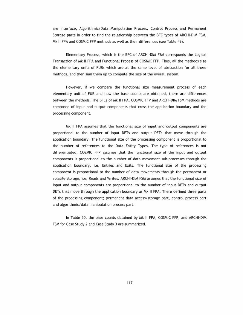
117

are Interface, Algorithmic/Data Manipulation Process, Control Process and Permanent

Storage parts in order to find the relationship between the BFC types of ARCHI-DIM FSM,

Mk II FPA and COSMIC FFP methods as well as their differences (see Table 49).

Elementary Process, which is the BFC of ARCHI-DIM FSM corresponds the Logical

Transaction of Mk II FPA and Functional Process of COSMIC FFP. Thus, all the methods size

the elementary units of FURs which are at the same level of abstraction for all these

methods, and then sum them up to compute the size of the overall system.

However, if we compare the functional size measurement process of each

elementary unit of FUR and how the base counts are obtained, there are differences

between the methods. The BFCs of Mk II FPA, COSMIC FFP and ARCHI-DIM FSM methods are

composed of input and output components that cross the application boundary and the

processing component.

Mk II FPA assumes that the functional size of input and output components are

proportional to the number of input DETs and output DETs that move through the

application boundary. The functional size of the processing component is proportional to

the number of references to the Data Entity Types. The type of references is not

differentiated. COSMIC FFP assumes that the functional size of the input and output

components is proportional to the number of data movement sub-processes through the

application boundary, i.e. Entries and Exits. The functional size of the processing

component is proportional to the number of data movements through the permanent or

volatile storage, i.e. Reads and Writes. ARCHI-DIM FSM assumes that the functional size of

input and output components are proportional to the number of input DETs and output

DETs that move through the application boundary as Mk II FPA. There defined three parts

of the processing component; permanent data access/storage part, control process part

and algorithmic/data manipulation process part.

In Table 50, the base counts obtained by Mk II FPA, COSMIC FFP, and ARCHI-DIM

FSM for Case Study 2 and Case Study 3 are summarized.

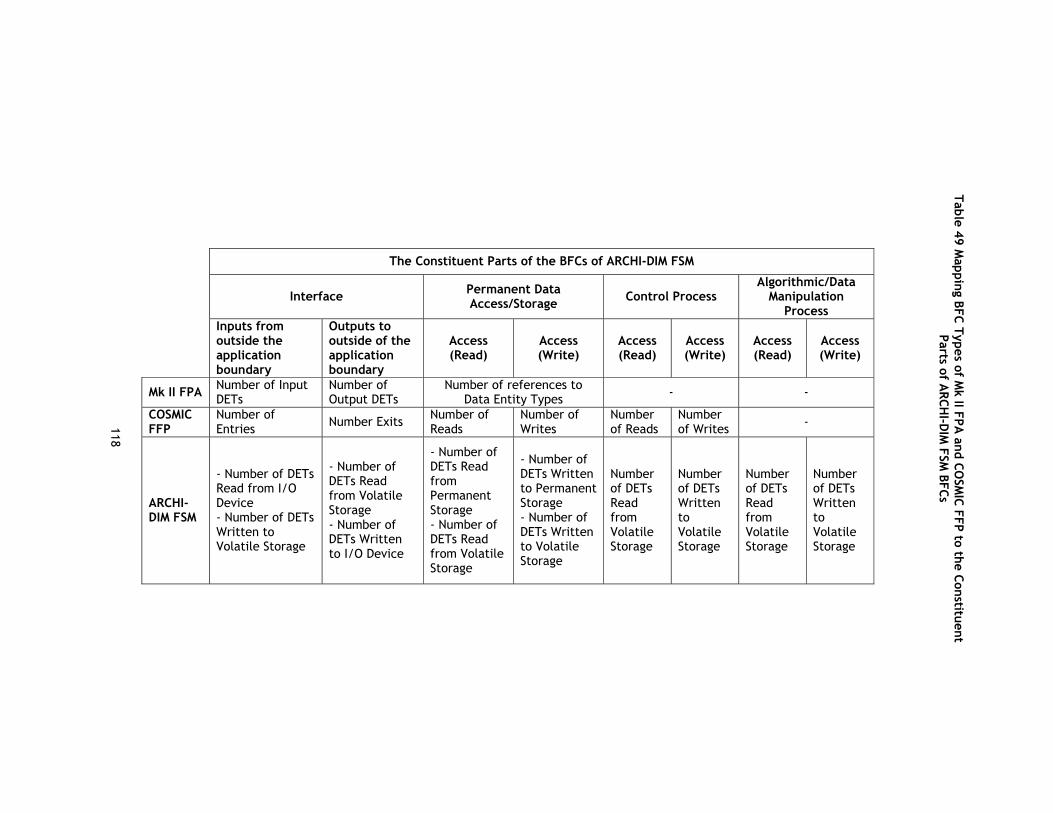
118

Table 49 Mapping BFC Types of Mk II FPA and COSMIC FFP to the Constituent Parts of ARCHI-DIM FSM BFCs

The Constituent Parts of the BFCs of ARCHI-DIM FSM

Interface Permanent Data Access/Storage Control Process

Algorithmic/Data Manipulation

Process Inputs from

outside the application boundary

Outputs to outside of the application boundary

Access (Read)

Access (Write)

Access (Read)

Access (Write)

Access (Read)

Access (Write)

Mk II FPA Number of Input DETs

Number of Output DETs

Number of references to Data Entity Types - -

COSMIC FFP

Number of Entries Number Exits Number of

Reads Number of Writes

Number of Reads

Number of Writes -

ARCHI-DIM FSM

- Number of DETs Read from I/O Device - Number of DETs Written to Volatile Storage

- Number of DETs Read from Volatile Storage - Number of DETs Written to I/O Device

- Number of DETs Read from Permanent Storage - Number of DETs Read from Volatile Storage

- Number of DETs Written to Permanent Storage - Number of DETs Written to Volatile Storage

Number of DETs Read from Volatile Storage

Number of DETs Written to Volatile Storage

Number of DETs Read from Volatile Storage

Number of DETs Written to Volatile Storage

Table 49 Mapping BFC Types of M

k II FPA and CO

SMIC FFP to the Constituent

Parts of ARCH

I-DIM

FSM BFCs

119

Table 50 Summary of the Base Counts obtained by Mk II FPA, COSMIC FFP and ARCHI-DIM FSM

ARCHI-DIM FSM Constituent Parts

Interface Permanent Data Access/Storage

Control Process

Algorithmic/ Data

Manipulation Process Project

No FSM Method

Read I/O

Write VS

Write I/O

Read VS

Read PS

Write VS

Write PS

Read VS

Read VS

Write VS

Read VS

Write VS

Mk II FPA 824 2,660 2,404 - - - -

COSMIC FFP 615 801 2,303 317 * * - - Project-

1 ARCHI-DIM FSM 474 474 2,512 2,509 3,333 3,357 334 766 1,092 142 1,002 1,141

Mk II FPA 283 126 592 - - - -

COSMIC FFP 206 51 588 100 * * - - Project-

2 ARCHI-DIM FSM 227 221 51 51 1 1 0 0 705 272 298 3,179

Mk II FPA 560 1,707 343 - - - -

COSMIC FFP 154 378 333 155 * * - - Project-

3 ARCHI-DIM FSM 558 558 1,705 1,705 1,884 1,884 627 627 1 0 160 137

* Since COSMIC FFP does not differentiate the functional size of control processes from permanent data access/storage part, in this table these figures shall be considered as part of the functional size of permanent data access/storage part.

Table 50 Summ

ary of the Base Counts obtained by Mk II FPA

, COSM

IC FFP and A

RCHI-D

IM FSM

120

The factors that cause the difference between the functional sizes of input and

output components of the BFCs, obtained by Mk II FPA and COSMIC FFP are discussed in

Section 4.2.2.4. If we compare how the base counts are obtained for the input and output

components of the BFCs of ARCHI-DIM FSM and Mk II FPA, the number of Read DETs from

I/O Device corresponds to the input DETs of Mk II FPA. The number of Write DETs to I/O

Device corresponds to Output DETs of Mk II FPA. The differences between these figures

(see Table 50) result from the assumption of Mk II FPA, which says that at least 1 input

DET and 1 output DET is present for a LT. In ARCHI-DIM FSM, there is no such assumption.

For the processing component of the BFCs, we compared the functional sizes of

the constituent parts of ARCHI-DIM FSM BFCs, i.e. algorithmic/data manipulation process,

control process and permanent data access/storage with Mk II FPA and COSMIC FFP.

Mk II FPA and COSMIC FFP are not designed to size Algorithmic / data manipulation

processes. Therefore, the functional sizes of these components could not be measured by

these methods (see Table 50). Although, COSMIC FFP takes into account Control processes

which are used to control the behavior of real-time systems in its functional size

measurement process, this method does not differentiate the size of these components

from the Permanent storage access / storage component. Therefore, the functional size of

this part is within the Permanent storage access / storage component and shall not be

considered as ‘0’.

The functional size of the Permanent data access/storage part of the BFCs of Mk II

FPA and COSMIC FFP are discussed in Section 4.2.2.4. COSMIC FFP measures the functional

sizes of the Permanent data access/storage part and Control process part by counting the

number of Read data movements and Write data movements. These parts are

differentiated in ARCHI-DIM FSM and the base counts are obtained at the level of DETs.

In Table 51, the ratio of the functional sizes and logical SLOC values of the

subsystems of Project-1 are given. The ratios of the functional sizes and SLOC Values of

the subsystems of Project-1 are given in Table 52. In Table 53, the ratios of logical SLOC

values to the functional sizes of the subsystems of Project-1 are given. We found these

ratios for the subsystems of Project-1, all of which were developed by the same group in

the same organization and coded in C++, so that the results could be compared. Project-2

and Project-3 were coded in different programming languages and were developed by

different teams.

121

In Table 54, the functional sizes of the subsystems of Project-1 obtained by Mk II

FPA and COSMIC FFP in Case Study 2.1 with respect to ARCHI-DIM FSM dimensions are

presented. In Table 55, the ratios of SLOC to Functional Size (Mk II FP and Cfsu) of the

Subsystems of Project-1 are given.

The variation of SLOC/Functional size (Mk II FP and Cfsu) ratio for the projects in

ISBSG dataset is discussed in Section 5.1.1.7. If we compare the values of these ratios with

the ratios obtained by ARCHI-DIM FSM, although the variation is smaller, we could not

conclude that separating the functionality types improved the ratio between SLOC and

functional size values.

Traditionally, we assume that these two metrics can be converted to each other by

multiplying one with an average ratio figure derived from numbers of projects. In other

words, we assumed that there is a linear relationship between these two metrics.

However, one of the reasons of this variation may be is that the relationship between

these two metrics being not linear. Another reason may be that there still exist some

issues on how the functionality is measured. In all FSM methods, we first identify the

elementary components of FURs, measure the functionality amount of each and then sum

them up them to compute the overall size of the system. Therefore, we measure the

amount of functionality at a fixed level of abstraction which is defined from the user’s

point of view. However, SLOC represents the size from the designer’s point of view. Based

on the type of functionality, a user might correspond to different sizes of software.

122

Table 51 The Functional Sizes (Mk II FP, Cfsu and ADfsu) and SLOC Values of the Subsystems of Project-1

Subsystem Interface

Functional Size (ADfsu)

Process Functional

Size (ADfsu)

Permanent Storage

Functional Size (ADfsu)

Functional Size

(Mk II FP)

Functional Size

(Cfsu)

Interface SLOC

Process SLOC

Permanent Storage SLOC

Total SLOC

A 5,105 2,620 7,082 4,374.24 3,505 4,615 6,202 1,326 12,143

B 544 464 400 435.24 279 967 2,161 321 3,449

C 320 293 332 350.68 252 1,409 2,184 321 3,914

Table 51 The Functional Sizes (Mk II FP, Cfsu and A

Dfsu) and SLO

C Values of the Subsystem

s of Project-1

123

Table 52 The Ratios of the Functional Sizes and SLOC Values of the Subsystems of Project-1

Subsystem

The Ratios of Interface

Functional Size (ADfsu)

The Ratios of Process

Functional Size (ADfsu)

The Ratios of

Permanent Storage

Functional Size (ADfsu)

The Ratios of Mk II FP

The Ratios of Cfsu

The Ratios of Interface

SLOC

The Ratios of Process SLOC

The Ratios of

Permanent Storage SLOC

The Ratios of

Total SLOC

A / B 9.38 5.65 17.71 10.05 12.56 4.77 2.87 4.13 3.52

A / C 15.95 8.94 21.33 12.47 13.91 3.28 2.84 4.13 3.10

B / C 1.70 1.58 1.20 1.24 1.11 0.69 0.99 1.00 0.88

Table 52 The Ratios of the Functional Size and SLOC Values of Subsystem

s of Project-1

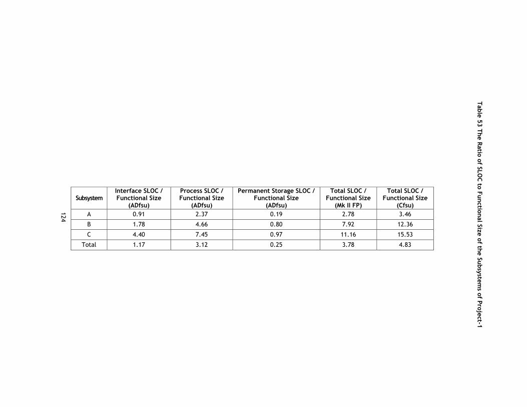
124

Table 53 The Ratio of SLOC to Functional Size of the Subsystems of Project-1

Subsystem Interface SLOC / Functional Size

(ADfsu)

Process SLOC / Functional Size

(ADfsu)

Permanent Storage SLOC / Functional Size

(ADfsu)

Total SLOC / Functional Size

(Mk II FP)

Total SLOC / Functional Size

(Cfsu) A 0.91 2.37 0.19 2.78 3.46

B 1.78 4.66 0.80 7.92 12.36

C 4.40 7.45 0.97 11.16 15.53

Total 1.17 3.12 0.25 3.78 4.83

Table 53 The Ratio of SLOC to Functional Size of the Subsystem

s of Project-1

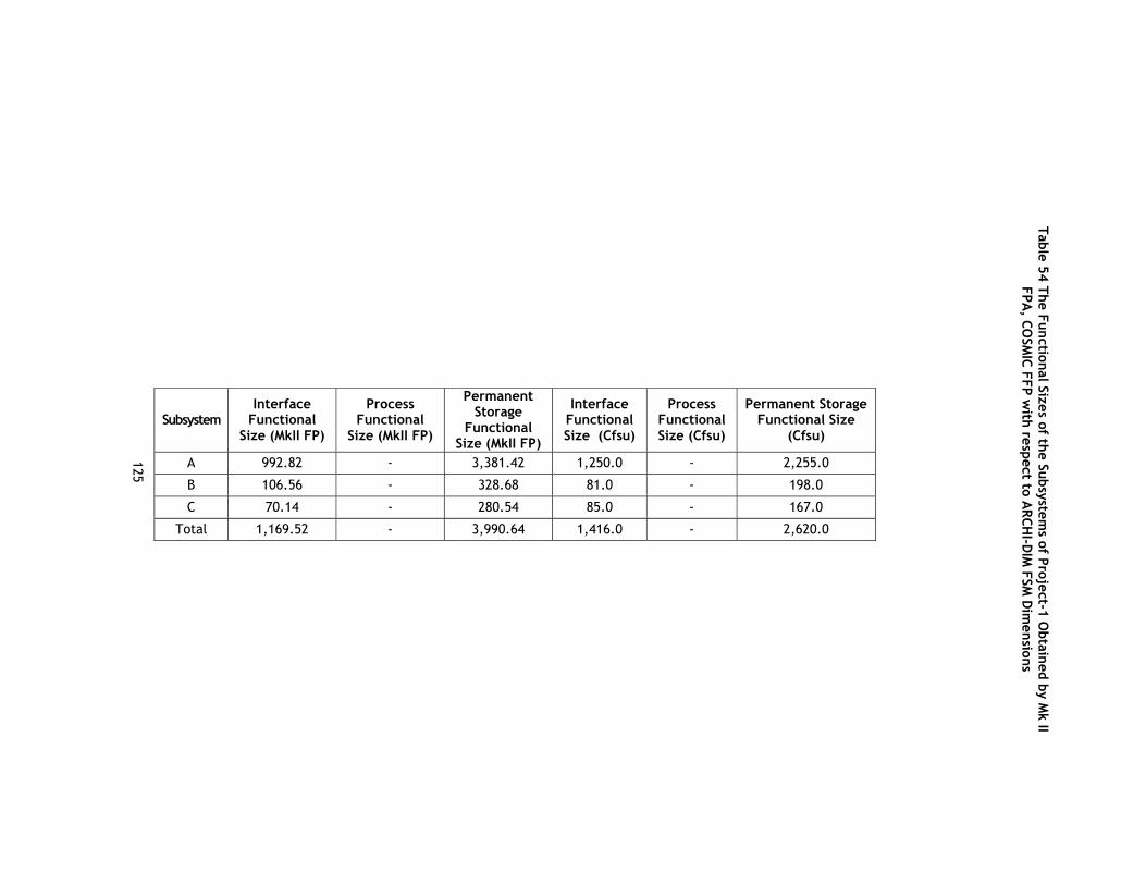
125

Table 54 The Functional Sizes of the Subsystems of Project-1 Obtained by Mk II FPA, COSMIC FFP with respect to ARCHI-DIM FSM Dimensions

Subsystem Interface

Functional Size (MkII FP)

Process Functional

Size (MkII FP)

Permanent Storage

Functional Size (MkII FP)

Interface Functional Size (Cfsu)

Process Functional Size (Cfsu)

Permanent Storage Functional Size

(Cfsu)

A 992.82 - 3,381.42 1,250.0 - 2,255.0

B 106.56 - 328.68 81.0 - 198.0

C 70.14 - 280.54 85.0 - 167.0

Total 1,169.52 - 3,990.64 1,416.0 - 2,620.0

Table 54 The Functional Sizes of the Subsystems of Project-1 O

btained by Mk II

FPA, CO

SMIC FFP w

ith respect to ARCH

I-DIM

FSM D

imensions

126

Table 55 The Ratios of SLOC to Functional Size (Mk II FP and Cfsu) of the Subsystems of Project-1

Subsystem Interface SLOC/ Functional Size

(MkII FP)

Process SLOC/ Functional Size

(MkII FP)

Permanent Storage SLOC/ Functional Size

(MkII FP)

Interface SLOC/ Functional Size

(Cfsu)

Process SLOC/ Functional Size

(Cfsu)

Permanent Storage SLOC/ Functional Size

(Cfsu) A 4.65 - 0.39 3.69 - 0.59

B 9.07 - 0.98 11.94 - 1.62

C 20.08 - 1.14 16.58 - 1.92

Total 5.98 - 0.49 4.94 - 0.75

Table 55 The Ratios of SLOC to Functional Size (M

k II FP and Cfsu) of the Subsystem

s of Project-1

127

If we analyze an example Elementary Processes, the reasons of this discussion

would be clearer:

BFC- 1 (Elementary Process or LT or Functional Process):

IF (“Map Option” selected AND State 1 AND

((‘ActivePage’ is “X” AND ‘X_Place’ is “A”) OR

(‘ActivePage’ is “Y” AND ‘X_Place’ is “A”) OR

(‘ActivePage’ is “Z” AND ‘X_Place’ is “A”) OR

(‘ActivePage’ is “V” AND ‘X_Place’ is “A”) OR

(‘ActivePage’ is “W” AND ‘X_Place’ is “A”) OR

(‘ActivePage’ is “M” AND ‘X_Place’ is “A”) AND

(Data “ABC” valid)

THEN (State 2 AND Output_1 (1 attribute) AND Output_2 (2 attributes) AND

Output_3 (1 attribute))

BFC- 2 (Elementary Process or LT or Functional Process):

IF (“Map Option” selected AND State 1 AND

((‘ActivePage’ is “X” AND ‘X_Place’ is “A”) OR

(‘ActivePage’ is “Y” AND ‘X_Place’ is “A”) OR

(‘ActivePage’ is “Z” AND ‘X_Place’ is “A”) OR

(‘ActivePage’ is “V” AND ‘X_Place’ is “A”) OR

(‘ActivePage’ is “W” AND ‘X_Place’ is “A”) OR

(‘ActivePage’ is “M” AND ‘X_Place’ is “A”) AND

(Data “ABC” valid) AND

(Data “KLM” valid)

THEN (State 2 AND Output_1 (1 attribute) AND Output_2 (2 attributes) AND

Output_3 (1 attribute), Output_4 (2 attribute))

According to the rules of all FSM methods as well as ARCHI-DIM FSM, these two

BFCs should be measured separately since these are regarded as being different with

respect to the user. Therefore, for these kinds of BFCs, which we encounter especially in

real-time systems, we measure very similar BFCs many times. This may increase the

functional size considerably. However, the SLOC corresponding to these BFCs does not

necessarily increase at the same rate. In addition, the design of the software may change

the SLOC amount considerably.

128

This is also true for ARCHI-DIM FSM. Although we separated the functionality types

in each Elementary Process, we measure the functionality amount of each after identifying

Elementary processes as in other FSM methods. Therefore, we suggest this as a future

improvement opportunity of ARCHI-DIM FSM.

One of the improvement suggestions of this thesis study, which is designating

functional size as a vector of measures for different types of functionality, motivated the

development of ARCHI-DIM FSM (see Section 3.2). The contribution of this classification

could be that the effort for each functionality type could also be estimated separately due

to the fact that the development effort for each might be different. High correlation

between functional size and effort is highly desired in order to define the relationship

between these attributes and estimate effort from the functional size. We determined the

correlation between the functional size measured by Mk II FPA, IFPUG FPA and COSMIC FFP

and the related efforts utilized for a number of projects in ISBSG dataset (see Section

5.1.1.6). Unfortunately, the correlation values are not high for IFPUG FPA and COSMIC

FFP. Although Mk II FPA shows high correlation results, the number of projects estimated

by Mk II FPA that exist in ISBSG dataset are not significant.

The low correlation values between a single functional size value, which is the sum

of the sizes of different types of functionalities, and the total effort is not surprising. The

effort required to develop different types of functionalities which have the same

functional sizes might be different. This is analogous to motorway construction in civil

engineering. The effort needed for 100 m outfall pipe work is different than the effort

needed for 100 m sewer pipelines. Therefore, combining the functional sizes of different

types of functionalities, for which the efforts required to develop each are very different,

to an average single value might have resulted in lower correlation between these

attributes.

In this thesis study, we suggest conducting experimental studies in order to find

the correlation between the size of each functionality type and the effort needed to

develop that type of functionality. This can pioneer new effort measurement methods.

However, this needs conducting case studies for projects the development effort values of

which are collected with respect to Interface, Process (Control and Algorithmic/Data

Manipulation) and Permanent Data Access/Storage parts. For most of the projects, this is

not available. Although, most of the time, the FURs are allocated to a three-tier

architecture consisting of these parts, the effort utilized to develop these components are

not collected on this basis.

129

We have this information only for Project-3 in Case Study 3.3 (see Table 46). The

user interface and the database components of this project are developed by using the

Internal Development Framework developed by the organization. Internal Development

Framework is a tool to reuse CRUDL processes in standard web applications. By this tool,

the interface and database components are generated in parallel. For the processing part,

Java is as the primary programming language. These parts are developed not only by

different teams but also using different technologies. Therefore, the productivity rates

for developing these different functionalities are different (see Table 48). By Mk II FPA,

the productivity rate is 1.61 whereas it is 2.12 for COSMIC FFP. By ARCHI-DIM FSM, the

productivity rates are 0.08 for the Interface part, 3.87 for the Process part and 0.13 for

the Permanent Data Access/Storage part.

This case study also showed that the designation of the functional size with

respect to these constituent parts also has an advantage of representing the application

domain of the software. As can be seen from Table 42, Table 44 and Table 47, the

functional size of the Interface and Permanent Data Access / Storage part is greater for

data-strong systems. For control-strong systems, the size of the Control Process part is

greater whereas for algorithm-strong systems, the Algorithmic Process part is greater.

Therefore, one can have an idea on the type of the software when the functional size

obtained by ARCHI-DIM FSM. The single index value obtained by other methods does not

give much information about the software application domain.

Another result of this case study is that ARCHI-DIM FSM method requires more

effort to measure the same system than by Mk II FPA and COSMIC FFP (see Table 56) and,

therefore, it is more time consuming. This is due to the fact that, among ARCHI-DIM FSM,

COSMIC FFP and MkII FPA methods, the level of granularity of ARCHI-DIM FSM is the lowest

one. Therefore, it requires much more information on the FURs than the other two

methods in order to be implemented.

Table 56 Efforts Utilized for Functional Size Measurement by MkII FPA, COSMIC FFP and ARCHI-DIM FSM

Case Study Name Effort Utilized by

Mk II FPA (person-hours)

Effort Utilized by COSMIC FFP

(person-hours)

Effort Utilized by ARCHI-DIM FSM (person-hours)

Case Study 2.1 71.38 56.50 99.50 Case Study 2.2 54.50 12.50 44.50 Case Study 2.3 23.33 12.58 34.25

130

The author of this thesis study is not involved in the measurement process of

ARCHI-DIM FSM for Case Study 3.3 in order to get objective feedback from another person

who is implementing this method for the first time. ARCHI-DIM FSM method is introduced

to this person by means of a measurement guideline (see Section 0). He implemented the

measurement process and the rules discussed in this guideline. The feedback provided by

the estimator is as follows (Yüceer, 2005):

- “ARCHI-DIM FSM puts more emphasis on control strong and function strong

systems as well as data strong systems.”

- “ARCHI-DIM FSM provides more freedom to measure different constituent parts

of the software independently.”

- “ARCHI-DIM FSM is much more flexible in identifying entities.”

- “By ARCHI-DIM FSM, it is possible to measure a software by parts (layers).”

- “Though ARCHI-DIM is more flexible in algorithmic statements, there is an

improvement opportunity to handle conditional statements in a more defined

way.”

- “ARCHI-DIM FSM is more time consuming than Mk II FPA and COSMIC FFP.”

- “The measurement guideline of ARCHI-DIM FSM method needs support by

examples.”

131

CHAPTER V

5 CONCLUSIONS

This chapter summarizes the contributions of this research and suggests future

research directions derived from the results and discovered during this research studies.

This research has dealt with the improvement opportunities of FSM methods and

development of a new FSM method. A comprehensive literature review is performed, the

data in ISBSG database are analyzed, and two case studies are conducted in order to

examine the conceptual and theoretical differences between FSM methods and to explore

the applicability of FSM methods to applications of different functional domains and at

different phases of the software development life cycle.

The first case study is a single-case study which was conducted to explore the

applicability of four estimation methods at different phases of the software development

life cycle. The second case study is a multiple-case study which involves three different

cases. The aim of this study was to explore the applicability of FSM methods to measure

the size of the projects of different functional domain types.

According to the findings of the literature review and the case studies, a number

of improvement opportunities are brought into light which are discussed in detail in the

following section. Based on these findings, some improvement suggestions are made on

the conceptual and theoretical basis of FSM and application domain applicability of FSM

methods. Accordingly, a new FSM method, called ARCHI-DIM FSM, is introduced.

A third multiple-case study is conducted and ARCHI-DIM FSM is implemented for

the same software products as in the second case study, sizes of which are measured by

Mk II FPA and COSMIC FFP methods. The improvement suggestions based on the new

method are evaluated and suggestions are made as future work.

132

5.1 Contributions to the Field of Software Engineering

This research has two significant contributions to the field of software

engineering; the identification of the improvement opportunities of FSM methods and the

development of a new FSM method, called ARCHI DIM FSM.

5.1.1 Improvement Opportunities of FSM Methods

The improvement opportunities of FSM methods are identified in the light of the

literature review and results of the three multiple-case studies conducted (see Section 4).

These improvement opportunities are discussed in the following sections.

5.1.1.1 Effects of Different Scales of FSM Methods on the Functional Size and Convertibility

In this thesis study, the effects of scales of different FSM methods on the

functional size and convertibility are explored due to the fact that the functional sizes of a

specific software product measured by different methods are different.

Although the FSM methods give roughly similar sizes on average, they have not in

general been designed to give similar sizes. In order to compare the measurement results

of one or more methods, convertibility of different measures has to be considered (Lother

and Dumke, 2001, Symons, 2001). In IEEE Std. 14143.1 (2000) it is stated that an FSM

Method should state its degree of convertibility to other sizing methods, which may be

full, or restricted by using an algorithm or mathematical model, or can not be converted

at all.

In this section, the effects of different scales of IFPUG FPA, Mk II FPA and COSMIC

FFP methods on the functional size based on the theoretical work discussed in Section 2.3

and the results of the case studies (see Sections 4.2.1.1 and 4.2.2.4) are explored.

Accordingly, the improvement opportunities on convertibility, which might guide to define

formulae for the conversion of functional sizes obtained by these methods to each other,

are discussed.

The reasons of the difference between the functional sizes arise from the

differences in BFC types of each method as well as how each FSM method measures these

components.

133

Symons (1999) studied the convertibility of Mk II FP and IFPUG FP to each other.

He stated that especially for large projects, the functional size of a software system

measured by Mk II FPA method would be greater than the one measured by IFPUG FPA

(Symons, 1999). Mk II FPA counts the number of references to each entity-type whereas

IFPUG counts entity types only once for an item of software. Although, for IFPUG FPA,

there is a second-order effect on the size of the External Input and Output processes

which reference them, this can not cope with the increasing difference between these two

methods as the project becomes larger. Accordingly, Symons (1999) defined the average

size relationships between Mk II FPA scale and IFPUG FPA scale in order to make it possible

to convert the sizes obtained by these two methods to each other.

In Case Study 1 (see 4.2.1), the functional size of a module of a subsystem

measured by IFPUG FPA is found to be 20.2 % smaller than the one by Mk II FPA. By using

the Symons’ conversion formula, the functional size of the module obtained by Mk II FPA is

converted from to IFPUG FPA scale. The difference between the functional sizes obtained

by the formula and the measured one is found to be about 13 %. This shows that although

this formula is very valuable, the assumptions used in this formula might result in error.

Symons (1999) stated that an ‘average conversion’ formula to convert COSMIC FFP

size to an IFPUG FPA size would be grossly misleading. Two main factors might give rise to

divergences between IFPUG and COSMIC FFP sizes. First one is that if the software being

measured has a high proportion of files which are not much referenced by the processes,

measurements made by IFPUG scale tend to result in higher sizes than by the COSMIC FFP

scale. The second factor arises from allocating size to each BFC whether within limited

ranges or with no upper limit. In IFPUG FPA, an External Input can have a size in the range

3 to 6 FP. In COSMIC FFP, there is no upper limit to the size of a functional process. If the

number of sub-processes in a Functional Process is high, the functional size obtained by

COSMIC FFP would be much higher. In Case Study 1 (see 4.2.1), the functional size

obtained by COSMIC FFP is 10.1 % greater than the one by IFPUG FPA.

In Mk II FP, the size of the processing component of an LT is defined to be

proportional to the number of Data Entity Types referenced. An entity reference in Mk II

FPA is generally equivalent to a Read or Write in COSMIC FFP (ISO/IEC 19761, 2003).

Therefore, the sizes of the processing component are roughly equivalent on both scales.

However, in Mk II FPA method, the size of the input and output components of a Logical

Transaction in Mk II FPA is defined to be proportional to the number of DETs in the input

and output components. In COSMIC FFP, the size of these components is defined to be

proportional to the number of Entries and Exits, but the number of DETs manipulated by

134

each sub-process is not taken into account. Therefore, for a specific software project with

exceptionally low proportion of DETs per Logical Transaction, the size estimated by Mk II

FPA would be lower than COSMIC FFP. On the other hand, if the Logical Transactions of a

project have exceptionally high proportion of DETs, this would result in higher sizes by Mk

II FP than by COSMIC FFP.

In Case Study 1, the functional size obtained by Mk II FPA is 11.2 % greater than

the one by COSMIC FFP. In Case Study 2, the functional sizes obtained by Mk II FPA are

greater than by COSMIC FFP for all three cases with a difference of 22 % in Case Study 2.1,

20 % in Case Study 2.2, and 24 % in Case Study 2.3.

The designers of COSMIC FFP stated that an ‘average conversion’ formula would

result a project to be under-sized or over-sized. We agree this statement by adding that

an average conversion formula of Mk II FPA measurement to COSMIC FFP is possible, but

the reverse is not true. If the system is estimated by Mk II FPA and the result is to be

converted to COSMIC FFP, we have detailed information on the number of data groups and

data movement types. However, when we want to convert COSMIC FFP size to Mk II FPA,

we do not have information on the number of DETs, i.e. we do not know if the system has

high or low number of DETs to decide on a formula.

The designers of COSMIC FFP states that there are practical and theoretical

reasons why convertibility of size is difficult (COSMIC, 2003). These are the lack of enough

data to develop statistically-based conversion formulae and having no definite conceptual

mapping between the BFC’s of one method and of the other to develop an exact

mathematically-based conversion formula.

Our concern about the reason why conversion of one size measure to another is

difficult is due to measuring the same attribute in different scales. Traditional activities

involved in measuring the functional size of software are stated to be; a) identifying BFCs

within the software, and b) assigning size units to each of these components in (Abran et

al., 2000). If the empirical relations about the “functional size” attribute were defined,

the different mappings of these relations to mathematical relations would not cause any

problem since the measures would be using the same scale types. Moreover, the problems

related to scale types used in FSM methods (Kitchenham, 1997) make conversion very

difficult or impossible, because the admissible transformation can not be defined based on

measures which do not obey the principles of measurement theory.

135

5.1.1.2 Effects of the Granularity Level on the FSM Process

Another improvement opportunity identified is related to the effects of the

granularity levels of the FSM methods on their FSM processes. The importance of the

granularity level comes from the fact that the software development projects that are not

providing any change in functionality but are changing how the functionality works can not

be measured by all methods. In addition, granularity level largely determines the required

effort for measurement and the timing of measurement during the software development

life cycle.

All ISO certified FSM methods are designed to be applicable after the FURs are

identified since the BFCs of all these methods are identified within FURs. However, the

abstraction levels of FURs may differ with respect to different projects. How the base

counts are obtained changes with respect to different methods. The granularity level of a

method depends on the measurement process of the method and at what detail level the

FURs shall be defined in order to make reliable measurement. Thus, the lower the

granularity level of the method, the more detailed the FURs shall be in order to obtain the

base counts. Since the FURs becomes more detailed in the later stages during the life

cycle, the applicability of the methods which are of low granularity are later in the life

cycle. And more effort is needed in order to pick that detailed information from FURs for

measurement.

In this thesis study, the granularity levels (GL) of Mk II FPA, COSMIC FFP, IFPUG

FPA and ARCHI-DIM FSM methods are analyzed with respect to their measurement

processes.

Mk II FPA method derives functional size by counting the input DETs, output DETs

and entity references whereas IFPUG FPA gives functional size value to each elementary

process depending on the complexity weight. This complexity weight depends on the

predetermined interval values of DETs. Therefore, the exact number of DETs is not

required in IFPUG FPA, i.e. determining the interval in which the number of DETs falls is

sufficient.

Thus, the granularity level of Mk II FPA measurement is lower than IFPUG FPA.

Therefore, the software development projects that are not providing any change in

functionality but are changing how the functionality works can be measured by Mk II FPA

but not by IFPUG FPA. With the IFPUG FPA method, the functional size of this kind of a

136

change would be “0” since no logical process-level functionality is being added, changed

or deleted.

COSMIC FFP method estimates functional size at a finer level of granularity than

IFPUG FPA, and a higher level of granularity than Mk II FPA. COSMIC FFP do not take into

account the number of DETs manipulated by each sub-process. It is stated that although

the movement of a single data attribute could be used as a sub-unit of measure,

measurements on a small sample of software in the field trials of COSMIC FFP indicated

that the average number of DETs per data movement did not vary much across the four

types of data movement (ISO/IEC 19761, 2003). Therefore, the COSMIC FFP unit of

measurement, 1 Cfsu, has been fixed at the level of one data movement. The users of this

method are warned to be careful when comparing the sizes of two different pieces of

software where the average number of DETs per data movement differs sharply across the

two pieces of software (ISO/IEC 19761, 2003). The granularity levels of these methods are

concluded as follows;

GL(IFPUG FPA) > GLCOSMIC FFP > GLMk II FPA

The granularity level affects the required effort for measurement. In Case Study 1,

the effort required to make measurement by Mk II FPA, IFPUG FPA, and COSMIC FFP was 35

person-hours, 24 person-hours, and 15 person-hours, respectively. In our implementation,

we utilized the greatest effort for Mk II FPA measurement since finding the number of

DETs takes longer. Since IFPUG FPA uses ranges for DETs and RETs while giving weights,

the effort needed to count the exact number of DETs and RETs decreased. Measurement

by COSMIC FFP took the shortest time. These differences are not only due to level of

granularity but also due to the order of measurement. We made measurement by Mk II

FPA, IFPUG FPA, and COSMIC FFP, consecutively. Therefore, we had more experience after

Mk II FPA measurement in finding the data groups and DETs while making measurement by

IFPUG FPA and COSMIC FFP. So, the efforts spent should not be directly compared to

determine the counting productivity.

In Case Study 2, for Case Study 2.1, the effort utilized to make the measurement

by Mk II FPA is 71.38 person-hours whereas it took 56.50 person-hours to make COSMIC FFP

measurement. For Case Study 2.2; the effort utilized for Mk II FPA measurement is 54.50

person-hours and it is 12.50 person-hours for COSMIC FFP measurement. For Case Study

2.3, the effort utilized to make the measurement by Mk II FPA is 23.33 person-hours and

by COSMIC FFP is 12.58 person-hours. Although it seems that we utilized greater effort for

Mk II FPA measurement in all of the cases of Case Study 2, we can not make such judgment

137

since we measured the projects by Mk II FPA and COSMIC FFP consecutively. Therefore, we

did not utilize extra effort to identify Functional Processes in COSMIC FFP since we had

already identified LTs in Mk II FPA.

The granularity level largely determines the timing of measurement during the

software development life cycle. Making measurement by the methods which have lower

granularity requires more information.

Thus, one of the conclusions of this study is that IFPUG FPA can be applied earlier

than COSMIC FFP and COSMIC FFP can be applied earlier than Mk II FPA during the life

cycle.

5.1.1.3 Estimation Timing

In order to be able to respond to contracts and plan in advance, the software

estimates should be performed early in the life cycle when we do not yet know the

sufficient details of the problem we are going to solve. In fact, when developing size

estimation models most of the recent researches have concentrated on the later phases of

software development, i.e. after the software requirements specification or preliminary

design phases. However, we require an estimation model that is reliable before the

detailed requirements are elicited.

Meli et al. (2000) pronounces this as a paradox: Size estimation would be necessary

when we do not have enough information and early estimation methods to obtain it. When

we can measure with the greatest accuracy, we do not need that information for effort

and duration prediction purposes any more.

In order to develop a model that can estimate size very early in the life-cycle,

process products available in the very early phases need to contain indicators of size. The

estimators in other engineering disciplines use construction standards and architectural

drawings to assess the size of the final product and to aid in developing initial project size

very early in the development process. However, the software engineering field lacks such

architectural form to assist estimators.

There are few size estimation methods in the literature. EFPA (Meli, 1997a; 1997b;

Conte et al., 2004) and E&Q COSMIC FFP (Meli et al., 2000; Conte et al., 2004) are the

examples of such methods.

138

In this thesis study, we applied EFPA, Mk II FPA and Jones Very Early Size Estimator

methods to estimate the size of a large software intensive military application, Request

for Proposal of which was also prepared by an approach we defined in an earlier study (see

Section 4.2.1). Among those, Jones Very Early Size Predictor is used to estimate the size of

the whole development project at the feasibility study phase. Mk II FPA is used to estimate

the size of the whole project after the detailed system-level functional requirements are

identified. Lastly, EFPA is used to estimate a module of that project at five consecutive

stages of the requirements analysis phase starting after the feasibility study until the

system level requirements are generated. The results of this study showed that all of the

three methods can be used for early size estimation considering their restrictions.

However, they all have their restrictions and early size estimation is an area demanding

further research. Therefore, developing early metrics and methods to make size

estimation early in the life cycle is an improvement opportunity.

5.1.1.4 Effects of Application Domain Types on the FSM Process

Another improvement opportunity identified is being related to the effects of the

application domain type on FSM process. Four kinds of software application domains are

defined in the literature; data-strong systems, control-strong systems, function-strong and

hybrid systems (see Section 2.2.2).

Unfortunately, there is not a single size measurement method which is designed to

measure all types of software. Each method has one or more target domains. The types of

application domains affect defining a method’s FSM process. The differences in the forms

of processing logic performed by each application type cause defining different BFC Types

to measure different components of software. Hybrid software systems (e.g. military

applications), which involves components of different application types such as real-time,

algorithmic and MIS components, requires an FSM method which can measure all types of

its components.

Maya et. al. (1998) discussed the differences between the software processes of

data-strong and real-time systems. A software process that generates data to be sent to

the user may have more than one sub-process. In data-strong systems (such as MIS), the

number of sub-processes does not add any important information to the functional size of

a given process since it is relatively constant across all processes of the same type.

Therefore, in IFPUG FPA, the number and nature of the sub-processes required to execute

an elementary process are not taken into account. However, control-strong systems such

139

as real-time systems shows a varying numbers of sub-processes per elementary process. In

addition, in data-strong systems, the data structure of logical files involves multiple

occurrences of a record, each of which has one or more fields. However, control-strong

systems involve a large number of single-occurrence control data as well as multiple

occurrence data. Therefore the developers of the COSMIC FFP method defined an

elementary unit of a FUR as a Functional Process, which is composed of data movement

sub-processes; Entry, Exit, Read, and Write (Maya et. al., 1998). This makes COSMIC FFP

method to be at a finer level of granularity than IFPUG FPA.

Function-strong systems are characterized by complex mathematical algorithms

and rules. They also involve conditional statements as control-strong systems. None of the

existing ISO certified FSM methods have been designed to measure the functionality of

these kinds of software processes.

In Case Study 2.1, there exist few mathematical algorithms and many conditional

statements. In Case Study 2.2, the mathematical algorithms and conditional statements

are dominating most of the LTs. And, there are a number of algorithmic operations in

Case Study 2.3, as well. We could not measure the functional size of mathematical

algorithms and conditional statements by Mk II FPA and COSMIC FFP in Case Study 2 since

these methods are not designed to measure the functional size of such components.

5.1.1.5 Conceptual and Theoretical Basis of FSM Methods

Other challenging improvement opportunities identified is related to improving the

conceptual and theoretical basis of FSM methods. Software development practitioners do

not have socially accepted basic size measures or on what constitutes product size. There

is a lack of good empirical relational systems and the software attributes (Hughes, 2000).

In addition, the mappings from the real world domain to the metric models are usually not

well defined.

Therefore, Fenton (1994; 1996) called for a rigor in software engineering through

measurement theory. The problems of function points related to scale types defined in

measurement theory were also summarized by Kitchenham (1997).

Xia (1998) suggested that clear definition of basic software concepts before

developing any serious measures was a basic requirement for any scientific theories. As for

software size, understanding of this attribute of software has become a concept which is

140

related to other attributes such as; the length of the code, functionality delivered to the

users, amount of reuse and complexity of the development (Fenton, 1996; Poel, 1998).

However, there are still arguments on the meaning of the terms “size”, “length”,

“complexity, and “functionality”.

Significant work has been carried out on the conceptual and theoretical basis of

measurement methods. Lokan (1999) studied the correlations between the BFC types in

FPA. Lokan (1999) analyzed a large data set - International Software Benchmarking

Standard Group (ISBSG) dataset to gain further insight into the correlations. ISBSG is one of

several opportunities that currently exist for gathering, retrieving, and sharing industry

data (Garmus, 2002). These kinds of data sets give opportunity to study not only the

conceptual and theoretical basis but the validations of both the existing methods and the

ones to be developed.

Kitchenham and Kansala (1993) and Jeffery and Stathis also studied the

correlations between the BFC types in FPA. Although some of their findings agree, they

found out different correlations in others. The outcomes of these studies showed that the

presence of these correlations cause to count the same things more than once in FPA.

Moreover, Kitchenham (1997) stated that the different results of studies on correlations

showed that, any predictive model based on the sum of the elements would not be stable

for different datasets.

Another study on the conceptual basis of FSM was initiated by the International

Standards Organization (ISO). ISO started a working group (ISO/IEC JTC1 SC7 WG12) on FSM

to establish common principles of the methods based on “functionality” metric and

brought a consistent terminology for the concepts related to size (ISO/IEC 14143-1, 1998).

In the first part of this standard (IEEE Std. 14143.1, 2000), “functional size” is

defined as “a size of the software derived by quantifying the Functional User

Requirements (FUR)”, “Base Functional Component (BFC)” is defined as “an elementary

unit of FUR defined by and used by an FSM Method for measurement purposes”, and “BFC

Type” is defined as “a defined category of BFCs”. It is also noted that there is some

controversy in the FSM community regarding the nature of “functional size” and cleared

that it “refers to the unique size obtained by applying a specific FSM method to a specific

set of software”, meaning that a piece of software has several functional sizes when

measured with different methods. This is due to different types of BFCs used by different

methods.

141

Therefore, in this thesis study, we based our work on the conceptual and

theoretical basis of these methods on the concepts defined in this standard. We compared

the three FSM methods; IFPUG FPA 4.1, Mk II FPA 1.3.1 and COSMIC FFP v.2.2 methods

according to ISO/IEC 14143-1 definitions (see Section 2.3). This standard requires that an

FSM method shall define its measurement process. A software product might have several

functional sizes when measured with different methods due to different types of BFCs

utilized by different methods. When applying an FSM method, we know what we are

counting and the differences between the FSM methods with respect to each other. What

we do not know is the relationship between BFC types of a method as well as between

different methods. This is especially important for the conversion of functional size

obtained by an FSM method to one another (see Section 5.1.1.1).

All three methods are widely-used and their theoretical bases are well published.

Among these, Abran (1994), Abran and Robillard (1994), Fenton (1996), and Kitchenham

(1997) discussed the fundamental flaws in the construction of these methods with respect

to measurement theory; especially issues related to scale types.

In this thesis study, we do not want to repeat the discussion on the scale types;

instead we discuss the improvement opportunities related to additivity of functional sizes

of different BFC Types. This is significant because although some methods improved issues

related to scale types, the addition of the resulting functional sizes of different BFC Types

is still problematic with respect to measurement theory.

For all three methods, the measurement function involves adding together the

functional sizes of different BFC types to obtain a total functional size. This is possible if

the assignment of weights to the various types of functions has transformed these

different BFC types into a single type. This problem of “additivity of the functional sizes of

different BFC Types” was mentioned by several authors. Abran stated the problem for

IFPUG FPA as “The additivity of functions poses a question, namely the relevance of

adding elements which are of different types and mean different things” (Abran, 1994).

Thus, he suggested that it would be more appropriate to call the final result an index

rather than a measurement of the size of an application and the FP count could be used as

a measurement or measurements of size able to reflect various points of view with

different units. All these dimensions in one or several subsets could be used to define and

measure a functional structure of software.

While discussing indirect measures, Fenton suggested “using vectors of measures

with rules for combining the vector elements into a larger, indirect measure” (Fenton,

142

1997). Kitchenham (1997) also mentioned this problem and suggested not adding or

combining the resulting counts together, instead using basic counts that are not weighted

as a vector of measures that describe the system”; such as a person’s clothing size is

defined as “chest size”, “waist size”, and “hip size”. Defining a vector of measures

instead of combining the resulting counts together to a single value is another

improvement opportunity.

5.1.1.6 Functional Size-Effort Correlation

Finding the relationship between the functional size and effort is another

improvement opportunity. Since one of the purposes of size measurement is to estimate

effort and cost, correlation between size and effort is highly desired for developing effort

and cost estimation methods.

During the measurement process of IFPUG FPA and Mk II FPA; after determining

the base counts, the complexity and contribution to functional size are determined. For

Mk II FPA, the weights turn counts of Input DETs, Output DETs, and Data Entity Type

references into equivalent measures. Unfortunately, there are no standard conversion

factors to equate inputs, outputs, and data entity type accesses; instead industry-average

weights are being used (Kitchenham, 1997). Another point stated by Symons that in Mk II

FPA the system size scale is taken to be related to the effort to analyze, design, and

develop the functions of the system (Symons, 1988). Therefore, these weights reflect the

effort rather than size.

The weights in IFPUG FPA reflects “the relative value of the function to the user

and determined by debate and trial”. In fact, the weights reflect the effort needed to

develop the corresponding functionality type.

COSMIC FFP method does not use weights for BFC types while calculating

functional size. Therefore, this method intended to separate functional size from effort.

Since one of the purposes of size measurement is to estimate effort, correlation

between size and effort is highly desired for developing estimation methods. In this thesis

study, we determined the correlation between the functional size measured by Mk II FPA,

IFPUG FPA and COSMIC FFP and the related efforts utilized for a number of projects in

ISBSG dataset (see Table 57).

143

Table 57 The Correlation between Functional Size and Effort

FSM Method Development Type

No of Projects

Correlation between size and effort

COSMIC FFP New 60 0.5560 IFPUG FPA New 720 0.4464 Mk II FPA New 15 0.9147

More work is needed to identify what kind of factors cause low correlation results

for these projects and to improve the functional size metrics accordingly. Although Mk II

FPA shows high correlation results, it should be noted that the number of projects

estimated by Mk II FPA that exist in ISBSG dataset are not significant.

5.1.1.7 Functional Size-SLOC Correlation

Another improvement opportunity identified is related to SLOC/Functional size

ratio, which have been the main driver of software project monitoring. Traditionally, we

assume that these two metrics can be converted to each other by multiplying one with an

average ratio figure derived from numbers of projects. In other words, we assume that

there is a linear relationship between these two metrics.

The size unit of measure is significant when using average ratios of SLOC to

functional size. In this thesis study, we analyzed SLOC to functional size ratios with the

data in the International Software Benchmarking Standard Group (ISBSG) dataset, which is

a large data set that exist for gathering, retrieving, and sharing industry data. Our aim

here is not to generalize these results statistically and to identify the relationship between

these two attributes, but rather to identify improvement opportunities related to

SLOC/functional size ratio, which have been the main driver of software project

monitoring. Therefore, we have not performed comprehensive statistical analyses.

Instead, we made analysis on the correlation between these attributes in order to identify

whether there is relationship between them or not and find the confidence interval for the

SLOC/functional size ratio in order to explore this ratio.

For the SLOC / functional size ratios, we calculated the confidence interval by the

following formula;

144

nzICσµ ±=. (1)

where, C.I. is the confidence interval, µ is the mean of the distribution of means,

σ is the standard deviation, n is the number of samples and z is the z-score for the

particular confidence interval of interest. For this analysis, we selected the desired

confidence interval as 90%. For the 90% confidence interval, the value of z is 1.64.

In ISBSG dataset, there are 15 new development projects, which are measured by

COSMIC FFP and SLOC of which also exist (see Table 58).

Table 58 The Ratio of SLOC to Functional Size (Cfsu)

Project ID SLOC Functional Size (Cfsu) SLOC / Cfsu Correlation SLOC –

Functional Size

1 1425 172 8.28 2 1350 470 2.87 3 1300 379 3.43 4 1250 183 6.83 5 1000 224 4.46 6 927 190 4.88 7 820 157 5.22 8 770 111 6.94 9 600 202 2.97 10 520 115 4.52 11 260 39 6.67 12 150 32 4.69 13 150 8 18.75 14 100 69 1.45

0.735

SLOC / Cfsu Min 1.05 Median 4.69 Max 18.75 Average 5.53 Std.Dev. 4.19

The application types of all these projects are Management Information Systems.

Unfortunately, the primary programming languages used for coding for these projects do

not exist in the dataset.

145

The correlation between SLOC and functional size is found as 0.735. The average

SLOC value is 722.8 with a minimum 100 and a maximum 1425. The average SLOC/size

ratio is 5.53 with a minimum value 1.04 and a maximum 18.75. The standard deviation is

4.19. These results show that, for any given project SLOC to functional size ratio would be

5.53 ± 1.77 within % 90 confidence interval. It should be noted that the size of these

projects are small and these results might not represent SLOC to Cfsu ratios for bigger

projects.

In ISBSG dataset, there are 1827 projects the functional sizes of which are

measured by IFPUG FPA. However, not all of these projects have the associated SLOC

values. For the projects having both functional size values and SLOC values, the ratios of

SLOC to functional size are given with respect to the primary programming languages

(SmallTalk, C++, Cobol, C) used for coding in Table 59, Table 60, Table 61 and Table 62.

Table 59 The Ratio of SLOC (SmallTalk) to Functional Size (IFPUG FP)

Project ID SLOC Functional Size (IFPUG FP) SLOC / IFPUG FP Correlation SLOC –

Functional Size 1 18700 320 58.44 2 7800 180 43.33 3 35089 700 50.13 4 111600 2600 42.92 5 82800 840 98.57 6 45100 1000 45.10 7 19800 800 24.75 8 30044 879 34.18 9 24700 990 24.95 10 19100 770 24.81 11 26800 1340 20.00 12 12800 320 40.00 13 31800 250 127.20 14 37000 350 105.71 15 11417 182 62.73

0.767

SLOC / IFPUG FP Min 20.00 Median 43.33 Max 127.20 Average 53.52 Std.Dev. 32.45

146

For 15 projects which are coded with SmallTalk, the correlation between SLOC and

functional size is found as 0.767. The average SLOC/size ratio is 53.52 with a minimum

value 20.00 and a maximum 127.20. The standard deviation is 32.45. These results show

that, for any given project coded with SmallTalk SLOC to functional size ratio would be

53.52 ± 13.74 within % 90 confidence interval.

Table 60 The Ratio of SLOC (C++) to Functional Size (IFPUG FP)

Project ID SLOC Functional Size (IFPUG FP) SLOC / IFPUG FP Correlation SLOC –

Functional Size 1 2800 106 26.42 2 6982 188 37.14 3 16000 238 67.23 4 36700 148 247.97 5 36700 200 183.50 6 36982 969 38.17 7 47000 250 188.00 8 47583 1291 36.86 9 48600 1305 37.24 10 49200 470 104.68 11 81800 320 255.63 12 82902 1658 50.00 13 229900 2010 114.38

0.726

SLOC / IFPUG FP Min 26.42 Median 67.23 Max 255.63 Average 106.71 Std.Dev. 84.24

For 13 projects which are coded with C++, the correlation between SLOC and

functional size is found as 0.726. The average SLOC/size ratio is 106.71 with a minimum

value 26.42 and a maximum 255.63. The standard deviation is 84.24. These results show

that, for any given project coded with C++, SLOC to functional size ratio would be 106.71

± 38.32 within % 90 confidence interval.

147

Table 61 The Ratio of SLOC (Cobol) to Functional Size (IFPUG FP)

Project ID SLOC Functional Size (IFPUG FP) SLOC / IFPUG FP Correlation SLOC –

Functional Size 1 1110 27 41.11 2 2354 22 107.00 3 3441 55 62.56 4 6328 171 37.01 5 6381 106 60.20 6 8404 367 22.90 7 11474 122 94.05 8 12428 404 30.76 9 16751 557 30.07 10 20569 342 60.14 11 24543 344 71.35 12 25072 319 78.60 13 26142 364 71.82 14 47136 1468 32.11 15 81095 760 106.70 16 83000 781 106.27 17 134216 1117 120.16

0.764

SLOC / IFPUG FP Min 22.90 Median 62.56 Max 120.16 Average 66.64 Std.Dev. 32.22

For 17 projects which are coded with Cobol, the correlation between SLOC and

functional size is found as 0.764. The average SLOC/size ratio is 66.64 with a minimum

value 22.90 and a maximum 120.16. The standard deviation is 32.22. These results show

that, for any given project coded with COBOL, SLOC to functional size ratio would be

66.64 ± 12.82 within % 90 confidence interval.

148

Table 62 The Ratio of SLOC (C) to Functional Size (IFPUG FP)

Project ID SLOC Functional Size (IFPUG FP) SLOC / IFPUG FP Correlation SLOC –

Functional Size 1 400 25 16.00 2 2000 300 6.67 3 2200 39 56.41 4 3200 79 40.51 5 4000 474 8.44 6 6000 168 35.71 7 6400 263 24.33 8 6500 194 33.51 9 10400 118 88.14 10 11300 257 43.97 11 12060 113 106.73 12 13990 335 41.76 13 14600 703 20.77 14 15000 777 19.31 15 16000 101 158.42 16 21900 170 128.82 17 26000 459 56.64 18 32000 213 150.23 19 58000 786 73.79 20 59000 118 500.00 21 60000 747 80.32 22 63000 551 114.34 23 63100 551 114.52 24 130000 202 643.56 25 300000 254 1181.10 26 334800 3354 99.82

0.665

SLOC / IFPUG FP Min 6.67 Median 65.22 Max 1181.10 Average 147.84 Std.Dev. 255.99

For 26 projects which are coded with C, the correlation between SLOC and

functional size is found as 0.665. The average SLOC/size ratio is 147.84 with a minimum

value 6.67 and a maximum 1181.10. The standard deviation is 255.99. These results show

that, for any given project coded with C, SLOC to functional size ratio would be 147.84 ±

82.33 within % 90 confidence interval.

149

We could not find the SLOC to Mk II FP ratios since the projects which are

measured by Mk II FPA have no associated SLOC values in the ISBSG dataset.

We found that the values of this ratio have high variation. ISBSG has a Comparative

Estimating Tool which is used to generate estimates of software project effort, delivery

rate, duration and speed of delivery. These estimates are determined from the projects

taken from the ISBSG repository that are deemed to be similar to the project for which the

estimate is required. The tool takes IFPUG FP as an input parameter. SLOC is not being

used for effort estimation which is expected due to the high variation between the ratios.

5.1.2 Development of a New FSM Method: ARCHI-DIM FSM

Another contribution of this research is making suggestions for some of the

significant improvement opportunities identified during this thesis work and accordingly

developing a new FSM method.

One of the improvement suggestions made is to use vectors of measures instead of

combining counts of different types of elements into a single value as also proposed by

Abran (1994), Fenton (1997) and Kitchenham (1997). By clarifying the concepts related to

functionality and by considering the software functional domain types and the software

architecture, we categorized functionality into four types; Interface, Control Process,

Algorithmic Process and Permanent Data Access/Storage functionalities.

Accordingly, a new FSM method, called ARCHI-DIM FSM, is introduced. Different

BFC Types and counting rules are defined for the Interface, Control Process, Algorithmic

Process and Permanent Data Access/Storage functionalities. ARCHI-DIM FSM method is an

initiative method for measuring different components of software which are of different

application domains.

One of the contributions of ARCHI DIM FSM method is that the effort for each

functionality type can be estimated separately since development effort for each might be

different. This is the case which we usually encounter especially if the developer wishes to

develop these “different” types of functionalities with different technologies and by

different teams. This is analogous to estimating effort and cost of a construction in civil

engineering. An example from Civil Engineering Standard Method of Measurement (CESMM,

1991) is Motorway Construction. The effort and cost related to the sizes of each item used

150

and the related effort to perform each process to construct that part are given in this

manual.

Case studies shall be conducted to find the correlation between the size of each

functionality type and the effort needed to develop it. This will pioneer new effort

estimation methods.

Defining guidelines in ARCHI-DIM FSM method to measure the size of algorithmic

operations and conditional statements is another contribution. The conditions on inputs to

produce different outputs have been considered to be related to functional complexity

(Tran-Cao, et al., 2004). However, the number of conditional statements increases the

number of SLOC as well as the effort needed to develop the software.

In Case Study 3, the size of the algorithmic operations and the conditional

statements, which can not be measured by Mk II FPA and COSMIC FFP, could be measured

by ARCHI-DIM FSM. The functional sizes of these components are found as 2,143 ADfsu,

3,477 ADfsu, and 297 ADfsu for Project-1, Project-2 and Project-3, respectively.

In addition, by ARCHI-DIM FSM, the functional size of the control components

which are used to control the behavior of real-time systems could be measured.

Accordingly, the functional size of these components is differentiated from the size of

permanent storage access/ storage component, for which the development efforts

required, might be different.

The designation of the functional size with respect to different types of

functionality also has an advantage of representing the application domain of the

software, i.e. data-strong, control-strong, algorithm-strong or hybrid system.

The variation of SLOC/Functional size (Mk II FP and Cfsu) ratio for the projects in

ISBSG dataset is discussed in Section 5.1.1.7. We compared the values of these ratios with

the ratios obtained by ARCHI-DIM FSM (see Table 53). Although the variation is smaller, we

could not conclude that separating the functionality types improved the ratio between

SLOC and functional size values. Therefore, this is identified as an improvement

opportunity.

151

5.2 Suggestions for Future Research

The following future research suggestions are derived and discovered during the

course of this research:

ARCHI-DIM FSM can be refined based on future case studies to be conducted to

explore the improvement opportunities of ARCHI-DIM FSM.

Future case studies shall be conducted to find the relation between the size of

each functionality type and the effort needed to develop that type of functionality. This

can pioneer new effort estimation methods.

The relationship between SLOC and functional size shall be analyzed in order to

identify new improvement opportunities for both metrics. One of the reasons of the

variation of SLOC/functional size may be is that the relationship between these two

metrics being not linear. Another reason may be that there are still some issues on how

the functionality is measured. During the measurement process of all FSM methods, the

elementary components of FURs identified first, then the functionality amount of each is

measured and then summed up to compute the overall size of the system. Therefore, the

amount of functionality is measured at a fixed level of abstraction which is defined from

the user’s point of view. However, SLOC represents the size from the designer’s point of

view. The functionality of very similar BFCs are measured separately although the

corresponding SLOC might not reflect this small change in functionality at the same rate.

These are the improvement opportunities identified related to the relationship between

SLOC and functional size.

An early estimation model for ARCHI-DIM FSM shall be developed. One of the

difficulties of software size estimation is the “Estimation Timing”. In order to develop a

model that can estimate size very early in the life-cycle, process products available in the

very early phases need to contain indicators related to “functional size” attribute. ARCHI-

DIM FSM shall be refined so that it can be used at different phases of the life cycle starting

from when high-level functional user requirements definition is available until the code is

available. We believe that an early representation model of a software system could be an

artifact that infers software system size. The Business Process Models (BPM) might serve as

architectural models from which some metrics that can predict software size early in the

life-cycle can be defined.

152

The abstraction levels of BFC definitions for FSM methods shall be explored and

new rules and definitions shall be defined. In ARCHI-DIM FSM, the highest level of

abstraction is defined in terms of the user's point of view, the second level in terms of the

segmentation of the functionality into parts and third level by identifying BFC Types of

each functionality type. Some issues are identified during the implementation of this

method (see Section 4.2.3.4). The same issues exist for the other FSM methods as well.

The level of abstraction of the BFCs, which are the elementary unit of FURs, affects

measuring the amount of functionality software provides to the user. Because, as the first

step, the BFCs are identified from the FURs in order to have a standard level of

abstraction regardless of the level of abstraction of the FURs. After that the functionality

of each BFC is measured and then summed up to compute the overall functionality.

Especially for real-time systems, same functionalities are being measured more than once

if required by the user in different BFCs. Defining new rules for identifying BFCs is another

improvement opportunity of FSM.

The amount of functionality to be provided to the user is measured by measuring

the SRS document as the entity which is an entity of the problem domain. When the design

document is the entity to be measured, new rules might be defined in order to reflect the

amount of functionality of the solution. Determining the relationship between the SLOC

values and design functional size, which are metrics related to solution domain, might be

more realistic.

Automation of ARCHI-DIM FSM shall be performed so that the effort required to

perform measurement would be decreased and the mistakes on counting could be avoided.

One of the most time consuming parts of the measurement process is the preparation of

the measurement catalogue due to the fact that for every Elementary Process, every BFC

Type and the counts of each should be recorded. Entering these values is not only time

consuming but also may result in making mistakes especially during counting.

153

6 BIBLIOGRAPHY

Abrahão, S. and Pastor, O. (2001). Estimating the Applications Functional Size from

Object-Oriented Conceptual Models, In International Function Points Users Group Annual Conference (IFPUG'01), Las Vegas, USA.

Abrahão, S., Poels, G., Pastor, O. (2004). Functional Size Measurement Method for Object-Oriented Conceptual Schemas: Design and Evaluation Issues, Working Paper, Faculty of Economics and Business Administration, Ghent University.

Abran, A. and Robillard, P.N.: Function Points (1994). A Study of Their Measurement Processes and Scale Transformations, Journal of Systems Software, No.25, pp.171-184.

Abran, A. (1994b). Analysis of the Measurement Process of Function Point Analysis, a PhD Thesis Submitted to Department of Electrical Engineering and Software Engineering, École Polytechnique De Montréal.

Abran, A., St-Pierre, D., Maya, M., Desharnais, J.M. (1998). Full Function Points for Embedded and Real-Time Software, UKSMA Fall Conference, London (UK), October 30-31.

Abran, A. (1999). COSMIC FFP 2.0: An Implementation of COSMIC Functional Size Measurement Concepts, FESMA’99, Amsterdam, 7 October.

Abran, A., Oligny, S., Symons, C., St-Pierre, D., Desharnais, J.M. (2000). Functional Size Measurement Methods – COSMIC FFP: Design and Field Trials, in FESMA-AEMES Software Measurement Conference 2000, Madrid, Spain.

Abran, A., Symons, C., Oligny, S. (2001). An Overview of COSMIC FFP Field Trial Results, ESCOM 2001, London, England, 2-4 April.

Abran, A., Fagg, P., Meli, R., Symons, C. (2002). ISO Transposition and Clarification of the COSMIC FFP Method of Functional Sizing, In Proceedings of the 12th International Workshop on Software Measurement (IWSM), October 7-9, 2002, Magdeburg, Shaker Publ., Aachen, pp. 33-42.

Albrecht, A. J. (1979). Measuring application development productivity, in Proceedings IBM Applications Development Symposium, Monterey, California, 14-17 October.

Albrecht, A.J. and Gaffney J. E. (1983). Software Function, Source Lines of Code, and Development Effort Prediction: A Software Science Validation, IEEE Transactions on Software Engineering, vol. SE-9, no. 6, November

Anda, B., Dreiem, H., Sjoberg, D. I. K., Jorgensen, M. (2001). Estimating Software Development Effort based on Use Cases-Experiences from Industry, 4th International Conference on the Unified Modeling Language (UML2001) Toronto, Canada, October 1-5, 2001, pp. 487-502, LNCS 2185, Springer-Verlag.

Arifoğlu, A. (1993). A Methodology for Software Cost Estimation, ACM SIGSOFT Software Engineering Notes, Vol. 18 , No.2, pp. 96-105.

154

Arnold, M. and Pedross, P. (1998). Software Size Measurement and Productivity Rating in a Large- Scale Software Development Department, Proceedings of the 1998 International Conference on Software Engineering. IEEE Computer Society, Los Alamitos, CA, USA.

Banker, R., Kauffman, R.J. , Wright, C , Zweig, D. (1994). Automating Output Size and Reuse Metrics in a Repository Based Computer Aided Software Engineering (CASE) Environment, IEEE Transactions on Software Engineering, Vol.20, No.3.

Bennett, W. R. (1996). Predicting Software System Development Effort very early in the Life-Cycle Using IDEF0 and IDEF1X Models, A PhD Dissertation Submitted to the Faculty of Mississippi State University.

Boehm, B.W. (1981). Software Engineering Economics, Prentice Hall, Englewood Cliffs, NJ.

Bozoki, G. J. (1993). An Expert Judgment Based Software Sizing Model, Journal of Parametrics, Vol. XIII, No 1.

Caldiera, G., Antoniol, G., Fiutem, R., Lokan, C. (1998). Definition and Experimental Evaluation for Object Oriented Systems, Proceedings of the 5th International Symposium on Software Metrics, Bethesda.

Card, D. N., El Emam, K., Scalzo, B. (2001). Measurement of Object Oriented Software Development Projects, Technical Report, Software Productivity Consortium, January.

Chidamber, S. R. and Kemerer, C. F. (1994). A Metric Suite for Object-Oriented Design, IEEE Transactions on Software Engineering, Vol. 20, No.6, pp. 476-493.

Computing Dictionary.(2005).http://computingdictionary.thefreedictionary.com/functionality,

CESMM - Civil Engineering Standard Method of Measurement. (1991). Thomas Telford Ltd., 3rd ed.

Conte, M. Iorio, T. Meli, R. Santillo, L. (2004). E&Q: An Early & Quick Approach to Functional Size Measurement Methods, in Software Measurement European Forum (SMEF), Rome, Italy.

Cristiansen, K., Fitsos, G.P., Smith, C.P. (1981). A Perspective on Software Science. IBM Systems Journal, Vol.20, No.4, pp.372-287.

DeMarco, T. (1982). Controlling Software Projects, Yourdon press, New York.

Demirörs, O., Gencel, Ç. Tarhan, A. (2003). Utilizing Business Process Models for Requirements Elicitation, 29th Euromicro Conference (EUROMICRO 2003), IEEE CS Press; pp. 409-412.

Demirörs, O. and Gencel, Ç. (2004). A Comparison of Size Estimation Techniques Applied Early in the Life Cycle, European Software Process Improvement Conference (EurSPI 2004), Springer Verlag Springer Lecture Notes in Computer Science (LNCS), pp.184-194.

Fairley, R. E. (1992). Recent Advances in Software Estimation Techniques, Proceedings of the 14th International Conference on Software Engineering, Melbourne, Australia, May 11-15, pp. 382-391.

Fenton, N. (1994). Software Measurement: A Necessary Scientific Basis, IEEE Transactions on Software Engineering, Vol.20, No.3, March

Fenton, N.E. and Pfleeger, S.L. (1996). Software Metrics: A Rigorous and Practical Approach, Second Edition, International Thomson Computer Press.

Forselius, P. (2004). Finnish Software Measurement Association (FiSMA), FSM Working Group: FiSMA Functional Size Measurement Method v. 1.1.

155

Garmus, D. and Herron, D. (2002). Estimating Software Earlier and More Accurately, CrossTalk, the Journal of Defense Software Engineering.

Glass, R.L. (2002). Facts and Fallacies of Software Engineering, Addison Wesley.

Halstead, M.H. (1977). Elements of Software Science, New York, Elsevier.

Henderson-Sellers, B. (1997). Corrigenda: Software Size Estimation of Object Oriented Systems, IEEE Transactions on Software Engineering, Vol. 23, No. 4., pp. 260-161.

Hughes, B. (2000). Practical Software Measurement, McGraw-Hill.

IFPUG: Counting Practices Manual - Release. 4.1.(1999). International Function Point Users Group, Westerville, OH.

IEEE Std. 14143.1-2000, Implementation Note for IEEE Adoption of ISO/IEC 14143-1:1998 - Information Technology- Software Measurement- Functional Size Measurement -Part 1: Definition of Concepts. (2000).

IEEE Std. 14143.1-2000, Implementation Note for IEEE Adoption of ISO/IEC 14143-1:1998 - Information Technology- Software Measurement- Functional Size Measurement -Part 1: Definition of Concepts. (2000).

ISBSG (International Software Benchmarking Standard Group) Dataset. (2004). http:// www.isbsg.org,

ISO/IEC 14143-1:1998 Information technology -- Software measurement -- Functional size measurement -- Part 1: Definition of concepts. (1998).

ISO/IEC 14143-2:2002 Information technology -- Software measurement -- Functional size measurement -- Part 2: Conformity evaluation of software size measurement methods to ISO/IEC 14143-1:1998. (2002).

ISO/IEC TR 14143-3:2003 Information technology -- Software measurement -- Functional size measurement -- Part 3: Verification of functional size measurement methods. (2003).

ISO/IEC TR 14143-4:2002 Information technology -- Software measurement -- Functional size measurement -- Part 4: Reference model. (2002).

ISO/IEC TR 14143-5:2004 Information technology -- Software measurement -- Functional size measurement -- Part 5: Determination of functional domains for use with functional size measurement. (2004).

ISO/IEC 20968, Software engineering - Mk II Function Point Analysis - Counting Practices Manual. (2002).

ISO/IEC 20926, Software engineering - IFPUG 4.1 Unadjusted FSM Method - Counting Practices Manual. (2003).

ISO/IEC 19761:2003: COSMIC Full Function Points Measurement Manual v. 2.2. (2003).

ISO/IEC 24570: Software engineering - NESMA Functional Size Measurement Method v.2.1 - Definitions and counting guidelines for the application of Function Point Analysis. (2005).

Jeffery, D.R. and Stathis, J. (1996). Function Point Sizing: Structure, Validity and Applicability, Journal of Empirical Software Engineering, Vol.1, No.1, pp.11-30.

Jones, T. C. (1987). A Short History of Function Points and Feature Points, Software Productivity Research Inc., USA.

Jones, T. C. (1998). Estimating Software Costs, McGraw-Hill.

Kammelar, J. (2000). A Sizing Approach for OO-environments, 4th International ECOOP Workshop on Quantitative Approaches in Object-Oriented Software Engineering.

156

Karner, G. (1993). Metrics for Objectory. Diploma thesis, University of Linköping, Sweden. No. LiTHIDA-Ex-9344:21.

Kauffman, R. and Kumar, R. (1997). Investigating Object-Based Metrics for Representing Software Output Size, Conference on Information Systems and Technology (CIST), in the INFORMS 1997 Annual Conference, San Diego.

Kauffman, R. and Kumar, R. (1993). Modeling Estimation Expertise in Object-Based CASE Environments, Stern School of Business Report, New York University.

Kemerer, C.F. (1987). An Empirical Validation of Software Cost Estimation Models, Communications of the ACM, Vol. 30, No.5, pp. 406-429.

Kitchenham, B. and Kansala, K. (1993). Inter-item Correlations among Function Points, In Proc. of the First International Metrics Symposium, May 21-22, IEEE Computer Society, pp. 11-14.

Kitchenham, B. (1997). The Problem with Function Points, IEEE Software, Vol. 14, Issue: 2, pp. 29-31.

Kitchenham, B, Pfleeger,S.L., Pickard, L.M., Jones, P.W., Hoaglin, D.C., El Emam, K., Rosenberg, J. (2002). Preliminary Guidelines for Empirical Research in Software Engineering, IEEE Transactions on Software Engineering, Vol. 28, No.8, pp. 721- 734.

Lewis, J. P. (2001). Large Limits to Software Estimation, ACM Software Engineering Notes, Vol. 26, No. 4, pp. 54-59.

Laranjeira, L. (1990). Software Size Estimation of Object Oriented Systems, IEEE Transactions on Software Engineering, Vol. 16, No. 5. pp.510-522.

Lokan, C.J. (1999). An Empirical Study of the Correlations Between Function Point Elements, Sixth IEEE International Symposium on Software Metrics, Boca Raton, Florida, November 04 – 06.

Lother, M. and Dumke, R.R. (2001). Points Metrics - Comparison and Analysis, In Proceedings of the International Workshop on Software Measurement (IWSM'01), Montréal, Québec, pp. 155-172.

Matson, J. E., Barret, B. E., Mellichamp, J. M. (1994). Software Development Cost Estimation Using Function Points, IEEE Transactions on Software Engineering, Vol. 20, No. 4, pp. 275-287.

Maya, M., Abran, A., Oligny, S., St-Pierre, D., Desharnais, J. M. (1998). Measuring the Functional Size of Real-Time Software, Proceedings of 1998 European Software Control and Metrics Conference, Maastricht, The Netherlands, pp. 191–199.

Meli, R. (1997a). Early and Extended Function Point: A New Method for Function Points Estimation, IFPUG-Fall Conference, September 15-19, Scottsdale, Arizona, USA.

Meli, R. (1997b). Early Function Points: a new estimation method for software projects, ESCOM 97, Berlin.

Meli, R. and Santillo L. (1999). Function Point Estimation Methods: A Comparative overview, FESMA 98-The European Software Measurement Conference, Amsterdam, October 6-8.

Meli, R., Abran, A., Ho, V.T., Oligny, S. (2000). On the Applicability of COSMIC FFP for Measuring Software Throughout Its Life Cycle, Proc. of the ESCOM-SCOPE 2000, April 2000, Munich, Germany, Shaker Publ., pp. 289-297.

Minkiewicz, A. F.: (2000). In Measuring Object Oriented Software with Predictive Object Points, PRICE Systems, L.L.C.

157

Miranda, E. (1999). Establishing Software Size Using the Paired Comparisons Method, Ericsson Research.

Miranda, E. (2001). Improving Subjective Estimates Using Paired Comparisons, IEEE Software, January / February, Vol.18, No.1, pp. 87-91.

Morisio, M., Stamelos, I., Spahos, V., Romano, D. (1999). Measuring Functionality and Productivity in Web-based Applications: A Case Study”, Proceedings of the sixth IEEE International Symposium on Software Metrics, November 04 – 06, pp. 111-118.

Netherlands Software Metrics Association (NESMA). (1997). Definitions and Counting Guidelines for the Application of Function Point Analysis, Version 2.0.

Oligny, S. and Abran, A. (1999). On the Compatibility Between Full Function Points and IFPUG Function Points , in Proceedings of the 10th European Software Control and Metric Conference (ESCOM SCOPE 99) , Herstmonceux Castle, England, pp. 10.

Oligny, S., Desharnais, J. M., Abran, A. (1999). A Method for Measuring the Functional Size of Embedded Software, 3rd International Conference on Industrial Automation, Montreal, Canada, June 7-9.

Pastor, O., Abrahão, S.M., Molina, J.C. and Torres, I. (2001). A FPA-like Measure for Object Oriented Systems from Conceptual Models, In Proceedings of the 11th International Workshop on Software Measurement - IWSM'01, Montréal, Canada, Shaker Verlag, pp. 51-69.

Paulk, M.C., Curtis, B., Chrissis, M.B., Weber, C. (1993). Capability Maturity Model for Software, version 1.1, Software Engineering Institute, CMU/SEI-93-TR-24, DTIC Number ADA263403.

Poel, G. (1998). Towards a Size Measurement Framework for Object Oriented Specifications, In Proceedings of the FESMA’98, Antwerp, Belgium, May 6-8, pp. 379-394.

Pressman, R.S. (1992). Software Engineering, A Practitioner’s Approach, Third Edition, McGraw Hill.

Putnam, L. H. And Fitzsimmons, A. (1979). Estimating Software Costs, Datamation, pp. 137-140.

Reifer, D.J. (1990). Asset-R: A Function Point Sizing Tool for Scientific and Real-time Systems, Journal of Systems and Software, Vol.11, No.3, pp.159-171.

Reifer, D.J. (2000). Web development: estimating quick-to-market software, IEEE Software, Vol.17, No.6, pp.57-64.

Ribu, K. (2001). Estimating Object Oriented Software Projects with Use Cases, Master of Science Thesis, University of Oslo.

Rollo, T. (2000). Sizing e-commerce, In Proceedings of the ACOSM 2000 – Australian Conference on Software Measurement, Sydney.

Rule, G. (1999). A Comparison of the Mark II and IFPUG Variants of Function Point Analysis [Online], http://www.gifpa.co.uk/library/Papers/Rule MK2IFPUG.html.

Rule, P. G. (2001). Using measures to understand requirements. In Proceedings of the ESCOM 2001, London, pp. 327-335.

Santillo, L. and Meli, R. (1998). Early Function Points: some practical experiences of use, ESCOM-ENCRESS 98, May 18, Roma, Italy.

Shepperd, M. and Cartwright, M. (1997). An Empirical Investigation of Object Oriented Software System, Technical Report No. TR 97/01, Dept. of Computing, Bournemouth University, UK.

158

Shepperd, M., Schofield, C., Kitchenham, B. (1996). Effort Estimation Using Analogy, In Proceedings of the 18th international conference on Software engineering (ICSE18), March 25-29, Berlin, Germany, pp.170-178.

Sırakaya, H.S. (2003). A Comparison of Object Oriented Size Evaluation Techniques, A MSc Thesis, Informatics Institute of the Middle East Technical University, Ankara, Turkey.

St-Pierre D., Maya M., Abran A., Desharnais J.-M., Bourque P. (1997). Full Function Points: Counting Practices Manual, Technical Report, Université du Québec à Montréal, Montréal, Canada.

Stutzke, R. D. (1998). Software Estimating Technology: A Survey, Science Applications International Corporation, Software Engineering 5th edition, pp.204-215.

Symons, C. R. (1988). Function Point Analysis: Difficulties and Improvements, IEEE Transactions on Software Engineering, Vol. 14, No. 1, pp.2-10.

Symons, C. (1999). Conversion between IFPUG 4.0 and MkII Function Points, Software Measurement Services Ltd., Version 3.0.

Symons, C. (2001). Come Back Function Point Analysis (Modernized) – All is Forgiven!), In Proceedings of the 4th European Conference on Software Measurement and ICT Control, FESMA-DASMA 2001, Germany pp. 413-426.

Tran-Cao, D., Lévesque, G., Meunier, J. (2004). Software Functional Complexity Measurement with the Task Complexity Approach, Intl. Conf. RIVF’04, February 2-5, Hanoi, Vietnam.

Teologlou, G. (1999). Measuring Object Oriented Software with Predictive Object Points, Shaker Publishing, ISBN 90-423-0075-2.

The Common Software Measurement International Consortium (COSMIC). (2003). FFP, version 2.2, Measurement Manual.

United Kingdom Software Metrics Association (UKSMA) (1998). MK II Function Point Analysis Counting Practices Manual Version 1.3.1.

Whitmire, S.A. (1992). 3D Function Points: Scientific and Real-time Extensions to Function Points, Pacific Northwest Software Quality Conference.

Whitten, J.L., Bentley, L.D., Dittman, K.C. (2001). System Analysis and Design Methods, McGraw-Hill, fifth edition.

Xia, F. (1998). On the Danger of Developing Measures Without Clarifying Concepts, Asia Pacific Software Engineering Conference, Taipei, Taiwan, December 02 – 04.

Yin, R.K. (1994). Case Study Research: Design and Methods, Applied Social Research Methods Series, Vol.5, 2nd ed., Sage Publications, Inc.

Yüceer, E. (2005). An Experimental Study on Software Size Measurement for Real-Time Safety Critical Software Systems, Technical Report-METU/II-TR-2005-35, Middle East Technical University, Informatics Institute, Ankara, Turkey.

159

APPENDICES

160

A

Template Measurement Catalogue Used for Mk II FPA Measurement

Logical Transaction

No

Logical Transaction

Input DET Explanation Output

DET Explanation Referenced Entity Number Explanation Mk II FP

A

PPEND

IX A

Tem

plate Measurem

ent Catalogue Used for M

k II FPA M

easurement

161

Template Measurement Catalogue Used for COSMIC FFP Measurement

Functional Process

No

Number Of Entries Explanation Number

Of Exits Explanation Number Of Reads Explanation Number

Of Writes Explanation Cfsu

Template M

easurement Catalogue U

sed for COSM

IC FFP Measurem

ent

162

a)

INTERFACE

Elementary Process

No

Number of Read DETs

(I/O) Explan.

Number of Write DETs (Volt.Strg.)

Explan. Number of Read DETs (Volt.Strg.)

Explan. Number of Write DETs

(I/O) Explan. INTERFACE

Functional Size

b)

Control PROCESS Component

Elementary Process

No

Number of Read DETs (Volt.Strg.)

Explan. Number of Write DETs (Volt.Strg.)

Explan. Control

PROCESS Functional Size

Template M

easurement Catalogue U

sed for ARCH

I-DIM

FSM M

easurement

163

c)

Algorithmic PROCESS Component

Elementary Process

No

Number of Read DETs (Volt.Strg.)

Explan. Number of Write DETs (Volt.Strg.)

Explan. Algorithmic

PROCESS Functional Size

d)

DB STORAGE / ACCESS Component

Elementary Process

No

Number of Read DETs

(Permanent Storage)

Explan. Number of Write DETs (Volt.Strg.)

Explan. Number of Read DETs (Volt.Strg.)

Explan.

Number of Write DETs (Permanent

Storage)

Explan.

Permanent Data Storage/ Access

Functional Size

Template M

easurement Catalogue U

sed for ARCH

I-DIM

FSM M

easurement (Cont.)

164

B

Case Study 1 – Module A1 - EFPA Estimation Catalogue (Stage 0 and Stage 1)

LD Comment F Comment MF Comment

1 1 LD (High Multiplicity) for BS (D/M) 1 1 MF (Medium) for BS (D/M'nin Yapılması) Level

0

1 1 LD (High Multiplicity) for CBS (D/M) 1 1 MF (Medium) for CBS (D/M'nin Yapılması)

1 1 LD (Simple) for BS (Md.1) 1 1 F (Small) for BS (Md.1) 1 1 MF (Small) for BS (Md. 2 (a,b,c,ç))

1 1 LD (High Multiplicity) for BS (Md.2 (a,b,c,ç,1 fonk.) 1

1 F (Medium) for BS (Md.2.d) 1

1 MF (Small) for CBS (Md. 2 (a,b,c,ç))

1 1 LD (High Multiplicity) for CBS (Md.2 (a,b,c,ç) 1

1 F (Medium) for CBS (Md.2.d)

1 1 LD (Low Multiplicity) for BS (Md.2.d) 1 1 F (Medium) for BS (Md.3,4,5)

1 1 LD (Low Multiplicity) for CBS (Md.2.d) 1 1 F (Medium) for CBS (Md.3,4,5)

1 1 LD (High Multiplicity) for BS (Md. 3,4,5)

Level 1

1 1 LD (High Multiplicity) for CBS (Md.3,4,5)

APPEN

DIX B

Case Study 1 – M

odule A1 - EFPA

Estimation Catalogue (Stage 0 and Stage 1)

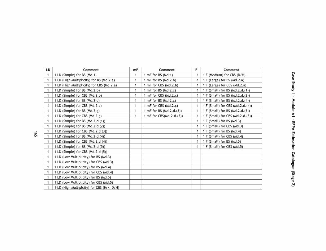
165

Case Study 1 – Module A1 - EFPA Estimation Catalogue (Stage 2)

LD Comment mF Comment F Comment 1 1 LD (Simple) for BS (Md.1) 1 1 mF for BS (Md.1) 1 1 F (Medium) for CBS (D/H) 1 1 LD (High Multiplicity) for BS (Md.2.a) 1 1 mF for BS (Md.2.b) 1 1 F (Large) for BS (Md.2.a) 1 1 LD (High Multiplicity) for CBS (Md.2.a) 1 1 mF for CBS (Md.2.b) 1 1 F (Large) for CBS (Md.2.a) 1 1 LD (Simple) for BS (Md.2.b) 1 1 mF for BS (Md.2.c) 1 1 F (Small) for BS (Md.2.d.(1)) 1 1 LD (Simple) for CBS (Md.2.b) 1 1 mF for CBS (Md.2.c) 1 1 F (Small) for BS (Md.2.d.(2)) 1 1 LD (Simple) for BS (Md.2.c) 1 1 mF for BS (Md.2.ç) 1 1 F (Small) for BS (Md.2.d.(4)) 1 1 LD (Simple) for CBS (Md.2.c) 1 1 mF for CBS (Md.2.ç) 1 1 F (Small) for CBS (Md.2.d.(4)) 1 1 LD (Simple) for BS (Md.2.ç) 1 1 mF for BS (Md.2.d.(3)) 1 1 F (Small) for BS (Md.2.d.(5)) 1 1 LD (Simple) for CBS (Md.2.ç) 1 1 mF for CBS(Md.2.d.(3)) 1 1 F (Small) for CBS (Md.2.d.(5)) 1 1 LD (Simple) for BS (Md.2.d (1)) 1 1 F (Small) for BS (Md.3) 1 1 LD (Simple) for BS (Md.2.d (2)) 1 1 F (Small) for CBS (Md.3) 1 1 LD (Simple) for CBS (Md.2.d (3)) 1 1 F (Small) for BS (Md.4) 1 1 LD (Simple) for BS (Md.2.d (4)) 1 1 F (Small) for CBS (Md.4) 1 1 LD (Simple) for CBS (Md.2.d (4)) 1 1 F (Small) for BS (Md.5) 1 1 LD (Simple) for BS (Md.2.d (5)) 1 1 F (Small) for CBS (Md.5) 1 1 LD (Simple) for CBS (Md.2.d (5)) 1 1 LD (Low Multiplicity) for BS (Md.3) 1 1 LD (Low Multiplicity) for CBS (Md.3) 1 1 LD (Low Multiplicity) for BS (Md.4) 1 1 LD (Low Multiplicity) for CBS (Md.4) 1 1 LD (Low Multiplicity) for BS (Md.5) 1 1 LD (Low Multiplicity) for CBS (Md.5) 1 1 LD (High Multiplcity) for CBS (Hrk. D/H)

Case Study 1 – Module A

1 - EFPA Estim

ation Catalogue (Stage 2)

166

LD Comment mF Comment fP Comment F Comment

1 1 LD (Simple) for BS (Md.1) 1 1 mF for BS (Md.1) 3 3 PI for BS (Md.3.(4) 1 1 F (Medium) for CBS (Hrk D/H'sı)

1 1 LD (Simple) for BS (Md.2.a.1) 1 1 mF for BS (Md.2.a.1) 1 1 PO for BS (Md.3.(4) 1 1 F (Medium) for BS (Md.2.a.3)

1 1 LD (Simple) for CBS (Md.2.a.1) 1 1 mF for CBS (Md.2.a.1) 1 1 PQ for BS (Md.3.(4) 1 1 F (Medium) for CBS (Md.2.a.3)

1 1 LD (Simple) for BS (Md.2.a.2) 1 1 mF for BS (Md.2.a.2) 16 16 PI for BS (Md.4.(2)) 1 1 F (Medium) for BS (Md.2.a.4)

1 1 LD (Simple) for CBS (Md.2.a.2) 1 1 mF for CBS (Md.2.a.2) 1 1 PO for BS (Md.4.(2)) 1 1 F (Medium) for CBS (Md.2.a.4)

1 1 LD (High Multiplicity) for BS (Md.2.a.3) 1 1 mF for BS (Md.2.b) 1

1 PQ for BS (Md.4.(2)) 1 1 F (Small) for BS (Md.2.d.(1))

1 1 LD (Low Multiplicity) for CBS (Md.2.a.3) 1 1 mF for CBS (Md.2.b) 1 1 F (Small) for BS (Md.2.d.(2))

1 1 LD (Low Multiplicity) for BS (Md.2.a.4) 1 1 mF for BS (Md.2.c) 1 1 F (Small) for BS (Md.2.d.(4))

1 1 LD (Low Multiplicity) for CBS (Md.2.a.4) 1 1 mF for CBS (Md.2.c) 1 1 F (Small) for CBS (Md.2.d.(4))

1 1 LD (Simple) for BS (Md.2.b) 1 1 mF for BS (Md.2.ç) 1 1 F (Small) for BS (Md.2.d.(5)) 1 1 LD (Simple) for CBS (Md.2.b) 1 1 mF for CBS (Md.2.ç) 1 1 F (Small) for CBS (Md.2.d.(5)) 1 1 LD (Simple) for BS (Md.2.c) 1 1 mF for BS (Md.2.d.(3)) 1 1 F (Small) for CBS (Md.3.(1))

1 1 LD (Simple) for CBS (Md.2.c) 1 1 mF for CBS (Md.2.d.(3)) 1 1 F (Small) for CBS (Md.3.(2))

1 1 LD (Simple) for BS (Md.2.ç) 1 1 F (Small) for CBS (Md.3.(3)) 1 1 LD (Simple) for CBS (Md.2.ç) 1 1 F (Medium) for BS (Md.4.(1)) 1 1 LD (Simple) for BS (Md.2.d (1)) 1 1 F (Small) for CBS (Md.4.(1)) 1 1 LD (Simple) for BS (Md.2.d (2)) 1 1 LD (Simple) for CBS (Md.2.d (3)) 1 1 LD (Simple) for CBS (Md.2.d (4)) 1 1 LD (Simple) for BS (Md.2.d (5))

Case Study 1 – Module A

1 - EFPA Estim

ation Catalogue (Stage 3)

167

LD Comment mF Comment fP Comment F Comment 1 1 LD (Simple) for CBS (Md.2.d (5)) 1 1 LD (Simple) for CBS (Md.3.(1)) 1 1 LD (Simple) for CBS (Md.3.(2)) 1 1 LD (Simple) for CBS (Md.3.(3)) 1 1 LD (Simple) for BS (Md.3.(4)) 1 1 LD (Low Multiplicity) for BS (Md.4) 1 1 LD (Low Multiplicity) for CBS (Md.4) 1 1 LD (Simple) for BS (Md.5.(1)) 1 1 LD (Simple) for CBS (Md.5.(1)) 1 1 LD (Simple) for CBS (Md.5.(2)) 1 1 LD (Simple) for BS (Md.5.(3)) 1 1 LD (Simple) for CBS (Md.5.(4)) 1 1 LD (Simple) for BS (Md.5.(5))

1 1 LD (High Multiplcity) for CBS (Hrk. D/H)

Case Study 1 – Module A

1 - EFPA Estim

ation Catalogue (Stage 3)

168

Case Study 1 – Module A1 - EFPA Estimation Catalogue (Stage 4) LD Comment mF Comment fP Comment F Comment

1 1 LD (Simple) for BS (Md.1) 1 1 mF for BS (Md.1) 3 3 PI for BS (Md.3.(4) 1 1 F (Medium) for CBS (Hrk D/H'sı)

1 1 LD (Simple) for BS (Md.2.a.1) 1 1 mF for BS (Md.2.a.1) 1 1 PO for BS (Md.3.(4) 1 1 F (Medium) for BS (Md.2.a.3)

1 1 LD (Simple) for CBS (Md.2.a.1) 1 1 mF for CBS (Md.2.a.1) 1 1 PQ for BS (Md.3.(4) 1

1 F (Medium) for CBS (Md.2.a.3)

1 1 LD (Simple) for BS (Md.2.a.2) 1 1 mF for BS (Md.2.a.2) 16 16 PI for BS (Md.4.(1)) 1 1 F (Medium) for BS (Md.2.a.4)

1 1 LD (Simple) for CBS (Md.2.a.2) 1 1 mF for CBS (Md.2.a.2) 16 16 PO for BS (Md.4.(1)) 1

1 F (Medium) for CBS (Md.2.a.4)

13 1 LD (Simple) for BS (Md.2.a.3 (a-j) 1 1 mF for BS (Md.2.b) 16 16 PQ for BS (Md.4.(1)) 1 1 F (Small) for BS (Md.2.d.(1))

3 1 LD (Simple) for CBS (Md.2.a.3 (a,b,c) 1 1 mF for CBS (Md.2.b) 4 4 PI for CBS (Md.4.(1)) 1 1 F (Small) for BS (Md.2.d.(2))

1 1 LD (Low Multiplicity) for BS (Md.2.a.4) 1 1 mF for BS (Md.2.c) 4 4 PO for CBS (Md.4.(1)) 1 1 F (Small) for BS (Md.2.d.(4))

1 1 LD (Low Multiplicity) for CBS (Md.2.a.4) 1 1 mF for CBS (Md.2.c) 4 4 PQ for CBS (Md.4.(1)) 1

1 F (Small) for CBS (Md.2.d.(4))

1 1 LD (Simple) for BS (Md.2.b) 1 1 mF for BS (Md.2.ç) 16 16 PI for BS (Md.4.(2)) 1 1 F (Small) for BS (Md.2.d.(5))

1 1 LD (Simple) for CBS (Md.2.b) 1 1 mF for CBS (Md.2.ç) 1 1 PO for BS (Md.4.(2)) 1 1 F (Small) for CBS (Md.2.d.(5))

1 1 LD (Simple) for BS (Md.2.c) 1 1 mF for BS (Md.2.d.(3)) 1 1 PQ for BS (Md.4.(2)) 1 1 F (Small) for CBS (Md.3.(1))

1 1 LD (Simple) for CBS (Md.2.c) 1 1 mF for CBS (Md.2.d.(3)) 1 1 F (Small) for CBS (Md.3.(2))

1 1 LD (Simple) for BS (Md.2.ç) 1 1 F (Small) for CBS (Md.3.(3)) 1 1 LD (Simple) for CBS (Md.2.ç)

1 1 LD (Simple) for BS (Md.2.d (1))

1 1 LD (Simple) for BS (Md.2.d (2))

1 1 LD (Simple) for CBS (Md.2.d (3))

1 1 LD (Simple) for BS (Md.2.d (4))

Case Study 1 – Module A

1 - EFPA Estim

ation Catalogue (Stage 4)

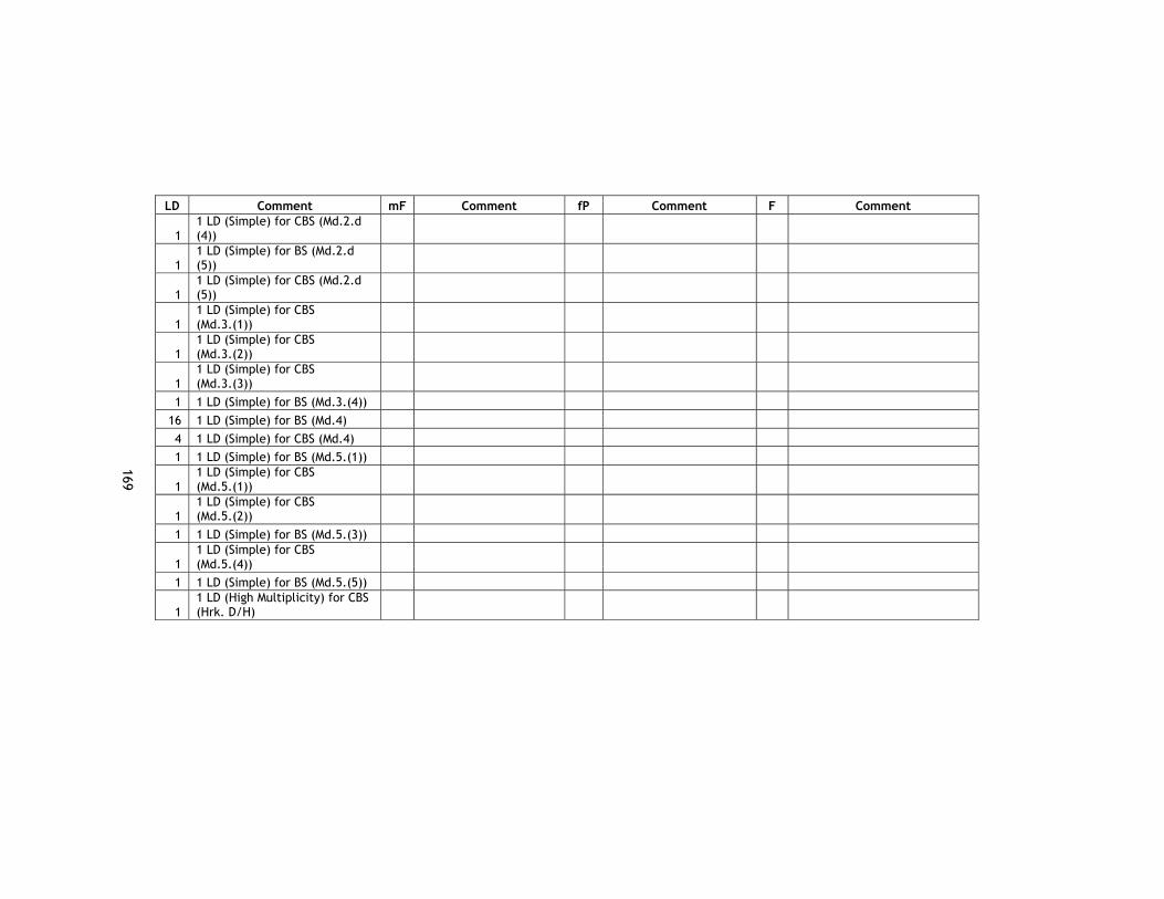
169

LD Comment mF Comment fP Comment F Comment

1 1 LD (Simple) for CBS (Md.2.d (4))

1 1 LD (Simple) for BS (Md.2.d (5))

1 1 LD (Simple) for CBS (Md.2.d (5))

1 1 LD (Simple) for CBS (Md.3.(1))

1 1 LD (Simple) for CBS (Md.3.(2))

1 1 LD (Simple) for CBS (Md.3.(3))

1 1 LD (Simple) for BS (Md.3.(4)) 16 1 LD (Simple) for BS (Md.4) 4 1 LD (Simple) for CBS (Md.4) 1 1 LD (Simple) for BS (Md.5.(1))

1 1 LD (Simple) for CBS (Md.5.(1))

1 1 LD (Simple) for CBS (Md.5.(2))

1 1 LD (Simple) for BS (Md.5.(3))

1 1 LD (Simple) for CBS (Md.5.(4))

1 1 LD (Simple) for BS (Md.5.(5))

1 1 LD (High Multiplicity) for CBS (Hrk. D/H)

170

Case Study 1 – Module A1 - EFPA Estimation Summary Results

Unadjusted EFP

Stage No Minimum Average Maximum

Stage 0 658 940 1,222

Stage 1 780 1,048 1,318

Stage 2 1,204 1,461 1,796

Stage 3 1,454 1,793 2,155

Stage 4 1,707 2,089 2,554

171

Case Study 1 – Module A1 – Mk II FPA & COSMIC FFP Estimation Catalogue Mk II FPA estimation catalogue COSMIC FFP estimation catalogue

LT No

No of Input DETs

No of Output DETs

Number of Data Element Types

Referenced MkII FP No of

Entries Number of Exits

Number of Reads

Number of Writes CFSU

203 1 1 2 4.16 1 1 1 1 4 205 53 16 32 88.02 16 32 0 16 64 205-1 56 56 64 153.28 34 19 32 32 117 206 20 1 21 46.72 20 1 20 1 42 206-1 23 23 1 20.98 4 4 2 2 12 209 39 6 12 44.10 6 12 0 6 24 209-1 42 42 24 75.12 9 9 12 12 42 210 6 1 11 22.00 1 1 10 1 13 210-1 9 9 4 14.20 4 4 2 2 12 211 4 1 22 39.10 1 1 21 1 24 211-1 7 7 4 12.52 4 4 2 2 12 212 2 1 51 86.08 1 1 50 1 53 212-1 1 1 51 85.50 1 1 50 1 53 212-2 5 5 4 10.84 4 4 2 2 12 212-3 4 4 4 10.00 4 4 2 2 12 213 4 1 12 22.50 1 1 11 1 14 213-1 7 7 4 12.52 4 4 2 2 12 213-2 2 1 9 16.36 2 2 8 2 14 213-3 5 5 4 10.84 6 5 4 4 19 215 4 1 12 22.50 1 1 11 1 14 215-1 7 7 4 12.52 4 4 2 2 12 221 5 1 22 39.68 1 17 21 1 40 221-1 8 8 4 13.36 4 4 2 2 12 222 6 1 9 18.68 1 9 8 1 19 222-1 9 9 4 14.20 4 4 2 2 12 223 5 1 11 21.42 1 11 10 1 23

Case Study 1 – Module A

1 – Mk II FPA

& CO

SMIC FFP Estim

ation Catalogue

172

Mk II FPA estimation catalogue COSMIC FFP estimation catalogue

LT No

No of Input DETs

No of Output DETs

Number of Data Element Types

Referenced MkII FP No of

Entries Number of Exits

Number of Reads

Number of Writes CFSU

223-1 8 8 4 13.36 4 4 2 2 12 224 1 1 12 20.76 1 10 11 1 23 224-1 4 4 4 10.00 4 4 2 2 12 225 1 1 1 2.50 1 1 0 1 3 225-1 4 4 4 10.00 4 4 2 2 12 226 2 1 5 9.72 1 1 4 1 7 226-1 5 5 4 10.84 4 4 2 2 12 227 1 1 1 2.50 1 1 0 1 3 227-1 4 4 4 10.00 4 4 2 2 12 228 9 2 4 12.38 2 4 0 2 8 228-1 12 12 8 23.36 6 5 4 4 19 231 9 2 4 12.38 2 4 0 2 8 231-1 12 12 8 23.36 6 5 4 4 19 232 3 1 2 5.32 1 2 0 1 4 232-1 6 6 4 11.68 4 4 2 2 12 234 6 1 22 40.26 1 2 20 1 24 234-1 9 9 4 14.20 4 4 2 2 12 234-2 9 2 23 43.92 2 2 21 2 27 234-3 12 12 8 23.36 6 5 4 4 19 240 1 1 10 17.44 1 1 9 1 12 240-1 1 1 10 17.44 1 1 9 1 12 240-2 4 4 4 10.00 4 4 2 2 12 240-3 4 4 4 10.00 4 4 2 2 12 240-4 8 2 20 38.36 2 25 20 2 49 240-5 11 11 8 22.52 6 5 4 4 19 247 3 1 12 21.92 1 8 8 1 18 247-1 6 6 4 11.68 4 4 2 2 12

173

Mk II FPA estimation catalogue COSMIC FFP estimation catalogue

LT No

No of Input DETs

No of Output DETs

Number of Data Element Types

Referenced MkII FP No of

Entries Number of Exits

Number of Reads

Number of Writes CFSU

248 3 1 21 36.86 1 18 12 1 32 248-1 6 6 4 11.68 4 4 2 2 12 248-2 5 5 36 63.96 18 18 36 18 90 248-3 5 1 3.16 1 1 18 1 21 248-4 8 8 4 13.36 4 4 2 2 12 270 9 2 4 12.38 2 2 2 2 8 270-1 12 12 8 23.36 6 5 4 4 19 271 64 1 3 42.36 1 2 2 1 6 271-1 67 67 8 69.56 4 4 2 2 12 278 177 1 59 200.86 58 58 58 58 232 TOTAL 845 438 747 1,844.00 319 398 563 245 1,525

174

Case Study 1 – Module A1 – IFPUG FPA Estimation Catalogue No of Data Functions Comment IFPUG

FP

No of Transactional

Functions Comment IFPUG FP

1 1 ILF (Simple) for BS (Md.1) 7 3 3 EI for BS (Md.3.(4) 18 1 1 ILF (Simple) for BS (Md.2.a.1) 7 1 1 EO for BS (Md.3.(4) 6 1 1 ILF (Simple) for CBS (Md.2.a.1) 7 1 1 EQ for BS (Md.3.(4) 6 1 1 ILF (Simple) for BS (Md.2.a.2) 7 16 16 EI for BS (Md.4.(1)) 96 1 1 ILF (Simple) for CBS (Md.2.a.2) 7 16 16 EO for BS (Md.4.(1)) 96 13 1 ILF (Simple) for BS (Md.2.a.3 (a-j) 91 16 16 EQ for BS (Md.4.(1)) 96 3 1 ILF (Simple) for CBS (Md.2.a.3 (a,b,c) 21 4 4 EI for CBS (Md.4.(1)) 24 1 1 ILF (Simple) for BS (Md.2.a.4) 7 4 4 EO for CBS (Md.4.(1)) 24 1 1 ILF (Simple) for CBS (Md.2.a.4) 7 4 4 EQ for CBS (Md.4.(1)) 24 1 1 ILF (Simple) for BS (Md.2.b) 7 16 16 EI for BS (Md.4.(2)) 96 1 1 ILF (Simple) for CBS (Md.2.b) 7 1 1 EO for BS (Md.4.(2)) 6 1 1 ILF (Simple) for BS (Md.2.c) 7 1 1 EQ for BS (Md.4.(2)) 6 1 1 ILF (Simple) for CBS (Md.2.c) 7 3 3 EI for BS (Md.1) 18 1 1 ILF (Simple) for BS (Md.2.ç) 7 2 2 EQ for BS (Md.1) 12 1 1 ILF (Simple) for CBS (Md.2.ç) 7 3 3 EI for BS (Md.2.a.1) 18 1 1 ILF (Simple) for BS (Md.2.d (1)) 7 2 2 EQ for BS (Md.2.a.1) 12 1 1 ILF (Simple) for BS (Md.2.d (2)) 7 3 3 EI for CBS (Md.2.a.1) 18 1 1 ILF (Simple) for CBS (Md.2.d (3)) 7 2 2 EQ for CBS (Md.2.a.1) 12 1 1 ILF (Simple) for BS (Md.2.d (4)) 7 3 3 EI for BS (Md.2.a.2) 18 1 1 ILF (Simple) for CBS (Md.2.d (4)) 7 2 2 EQ for BS (Md.2.a.2) 12 1 1 ILF (Simple) for BS (Md.2.d (5)) 7 3 3 EI for CBS (Md.2.a.2) 18 1 1 ILF (Simple) for CBS (Md.2.d (5)) 7 2 2 EQ for CBS (Md.2.a.2) 12 1 1 ILF (Simple) for CBS (Md.3.(1)) 7 3 3 EI for BS (Md.2.b) 18 1 1 ILF (Simple) for CBS (Md.3.(2)) 7 2 2 EQ for BS (Md.2.b) 12 1 1 ILF (Simple) for CBS (Md.3.(3)) 7 3 3 EI for CBS (Md.2.b) 18 1 1 ILF (Simple) for BS (Md.3.(4)) 7 2 2 EQ for CBS (Md.2.b) 12

Case Study 1 – Module A

1 – IFPUG

FPA Estimation Catalogue

175

No of Data Functions Comment IFPUG

FP

No of Transactional

Functions Comment IFPUG FP

16 1 ILF (Simple) for BS (Md.4) 112 3 3 EI for BS (Md.2.c) 18 4 1 ILF (Simple) for CBS (Md.4) 28 2 2 EQ for BS (Md.2.c) 12 1 1 ILF (Simple) for BS (Md.5.(1)) 7 3 3 EI for CBS (Md.2.c) 18 1 1 ILF (Simple) for CBS (Md.5.(1)) 7 2 2 EQ for CBS (Md.2.c) 12 1 1 ILF (Simple) for CBS (Md.5.(2)) 7 3 3 EI for BS (Md.2.ç) 18 1 1 ILF (Simple) for BS (Md.5.(3)) 7 2 2 EQ for BS (Md.2.ç) 12 1 1 ILF (Simple) for CBS (Md.5.(4)) 7 3 3 EI for CBS (Md.2.ç) 18 1 1 ILF (Simple) for BS (Md.5.(5)) 7 2 2 EQ for CBS (Md.2.ç) 12 29 EIF (external interface files) 145 3 3 EI for BS (Md.2.d.(3)) 18 2 2 EQ for BS (Md.2.d.(3)) 12 3 3 EI for CBS (Md.2.d.(3)) 18 2 2 EQ for CBS (Md.2.d.(3)) 12 3 3 EI for BS (Md.2.d.(1) 18 2 2 EQ for BS (Md.2.d.(1) 12 3 3 EI for BS (Md.2.d.(2) 18 2 2 EQ for BS (Md.2.d.(2) 12 3 3 EI or BS (Md.2.d.(4) 18 2 2 EQ or BS (Md.2.d.(4) 12 3 3 EI for CBS (Md.2.d.(4) 18 2 2 EQ for CBS (Md.2.d.(4) 12 3 3 EI for BS (Md.2.d.(5) 18 2 2 EQ for BS (Md.2.d.(5) 12 3 3 EI for CBS (Md.2.d.(5) 18 2 2 EQ for CBS (Md.2.d.(5) 12 3 3 EI for CBS (Md.3.(1) 18 2 2 EQ for CBS (Md.3.(1) 12 3 3 EI for CBS (Md.3.(2) 18

176

No of Data Functions Comment IFPUG

FP

No of Transactional

Functions Comment IFPUG FP

2 2 EQ for CBS (Md.3.(2) 12 3 3 EI for CBS (Md.3.(3) 18 2 2 EQ for CBS (Md.3.(3) 12 39 39 EI for BS (Md.2.a.3) 234 26 26 EQ for BS (Md.2.a.3) 156 9 9 EI for CBS (Md.2.a.3) 54 6 6 EQ for CBS (Md.2.a.3) 36 3 3 EI for BS (Md.2.a.4) 18 2 2 EQ for BS (Md.2.a.4) 12 3 3 EI for CBS (Md.2.a.4) 18 2 2 EQ for CBS (Md.2.a.4) 12

Total functional size 2,305 FP

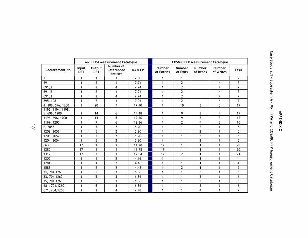
177

C

Mk II FPA Measurement Catalogue COSMIC FFP Measurement Catalogue

Requirement No Input DET

Output DET

Number of Referenced

Entities Mk II FP Number

of Entries Number of Exits

Number of Reads

Number of Writes Cfsu

3 1 1 1 2.50 1 1 2 691 1 2 4 7.74 1 2 4 7 691_1 1 2 4 7.74 1 2 4 7 691_2 1 2 4 7.74 1 2 4 7 691_3 1 2 4 7.74 1 2 4 7 695, 108 1 7 4 9.04 1 2 4 7 4, 108, 696, 1200 1 20 7 17.40 1 10 3 5 19 1195, 1194, 1198, 5, 696, 1200 1 14 6 14.18 1 9 3 4 17 1196, 696, 1200 1 13 5 12.26 1 9 3 3 16 1199, 1200 1 7 6 12.36 1 2 4 3 10 6, 2055 1 5 2 5.20 1 1 2 1 5 1202, 2056 1 5 2 5.20 1 1 2 1 5 1203, 2057 1 5 2 5.20 1 1 2 1 5 1204, 2054 1 5 2 5.20 1 1 2 1 5 663 17 1 1 11.78 17 1 1 1 20 1280 17 1 1 11.78 17 1 1 1 20 1317 17 2 1 12.04 17 2 1 1 21 1205 1 1 2 4.16 1 1 1 1 4 1281 1 1 2 4.16 1 1 1 1 4 1588 1 2 2 4.42 1 2 1 1 5 31, 704,1260 1 5 3 6.86 1 1 3 1 6 33, 704,1260 1 5 3 6.86 1 1 3 1 6 35, 704,1260 1 5 3 6.86 1 1 3 1 6 681, 704,1260 1 5 3 6.86 1 1 3 1 6 671, 704,1260 1 1 4 7.48 1 1 4 1 7

APPEN

DIX C

Case Study 2.1 - Subsystem

A - M

k II FPA and CO

SMIC FFP M

easurement Catalogue

178

Mk II FPA Measurement Catalogue COSMIC FFP Measurement Catalogue

Requirement No Input DET

Output DET

Number of Referenced

Entities Mk II FP Number

of Entries Number of Exits

Number of Reads

Number of Writes Cfsu

673, 704,1260 1 1 4 7.48 1 1 4 1 7 675, 704,1260 1 1 4 7.48 1 1 4 1 7 678, 704,1260 1 1 4 7.48 1 1 4 1 7 1250 1 1 1 2.50 1 1 1 3 25, 698 1 2 3 6.08 1 1 3 1 6 27, 699 1 2 3 6.08 1 1 3 1 6 1941, 1747 1 2 3 6.08 1 1 3 1 6 29, 699 1 2 3 6.08 1 1 3 1 6 677, 697 1 2 3 6.08 1 1 3 1 6 1261, 697 1 2 3 6.08 1 1 3 1 6 711, 1633 1 2 3 6.08 1 1 3 1 6 714, 692 1 2 3 6.08 1 1 3 1 6 1942 1 2 3 6.08 1 1 3 1 6 713, 692 1 2 3 6.08 1 1 3 1 6 712, 1747 1 2 3 6.08 1 1 3 1 6 37, 1747 1 2 3 6.08 1 1 3 1 6 38, 1206 1 2 3 6.08 1 1 3 1 6 39, 1207 1 2 3 6.08 1 1 3 1 6 1943 1 2 3 6.08 1 1 3 1 6 683, 1207 1 2 3 6.08 1 1 3 1 6 1262, 1244 1 2 3 6.08 1 1 3 1 6 1263, 1244 1 2 3 6.08 1 1 3 1 6 1264, 1245 1 2 3 6.08 1 1 3 1 6 1265, 702 1 2 3 6.08 1 1 3 1 6 1944 1 2 3 6.08 1 1 3 1 6 40, 702 1 2 3 6.08 1 1 3 1 6 1266, 701 1 2 3 6.08 1 1 3 1 6

179

Mk II FPA Measurement Catalogue COSMIC FFP Measurement Catalogue

Requirement No Input DET

Output DET

Number of Referenced

Entities Mk II FP Number

of Entries Number of Exits

Number of Reads

Number of Writes Cfsu

1267, 701 1 2 3 6.08 1 1 3 1 6 1295 1 1 3 5.82 1 3 1 5 1980 1 1 3 5.82 1 3 1 5 1296 1 1 3 5.82 1 3 1 5 1297 1 1 3 5.82 1 3 1 5 1981 1 1 3 5.82 1 3 1 5 1298 1 1 3 5.82 1 3 1 5 1299 1 1 3 5.82 1 3 1 5 1982 1 1 3 5.82 1 3 1 5 1300 1 1 3 5.82 1 3 1 5 1301 1 1 3 5.82 1 3 1 5 1983 1 1 3 5.82 1 3 1 5 1302 1 1 3 5.82 1 3 1 5 52 1 1 6 10.80 1 2 2 5 54 1 1 6 10.80 1 2 2 5 56 1 1 6 10.80 1 2 2 5 689 1 1 6 10.80 1 2 2 5 1663 1 1 5 9.14 1 1 4 6 1318, 1251 1 1 4 7.48 1 1 4 2 8 1319, 664 1 1 4 7.48 1 1 4 2 8 1320, 15 1 1 4 7.48 1 1 4 2 8 1321,13 1 1 4 7.48 1 1 4 2 8 1322, 666 1 1 4 7.48 1 1 4 2 8 1323, 17 1 1 4 7.48 1 1 4 2 8 1324, 1252 1 1 4 7.48 1 1 4 2 8 1325, 19 1 1 4 7.48 1 1 4 2 8 75 1 3 2 4.68 1 3 2 6

180

Mk II FPA Measurement Catalogue COSMIC FFP Measurement Catalogue

Requirement No Input DET

Output DET

Number of Referenced

Entities Mk II FP Number

of Entries Number of Exits

Number of Reads

Number of Writes Cfsu

76 1 3 2 4.68 1 3 2 6 78 1 3 2 4.68 1 3 2 6 892 1 9 3 7.90 1 8 3 12 80, 741 1 31 2 11.96 1 23 2 26 81, 741 1 16 2 8.06 1 8 2 11 742, 741 1 16 2 8.06 1 8 2 11 715, 741 1 16 2 8.06 1 8 2 11 165 1 2 1 2.76 1 2 1 4 167 1 2 1 2.76 1 2 1 4 92 2 1 3 6.40 1 1 3 5 1083 1 1 3 5.82 1 1 3 1 6 1933 1 1 3 5.82 1 1 3 1 6 85, 87 1 3 13 22.94 1 1 12 2 16 85, 88 1 3 13 22.94 1 1 12 2 16 86, 696 1 7 3 7.38 1 7 2 2 12 740, 696 1 7 4 9.04 1 7 3 2 13 89, 2166, 2163 1 20 5 14.08 1 1 4 1 7 91, 87 1 3 12 21.28 1 1 11 2 15 91, 88 1 3 12 21.28 1 1 11 2 15 100 1 8 9 17.60 1 1 9 11 101 1 5 9 16.82 1 1 9 11 102 1 8 9 17.60 1 1 9 11 103 1 5 9 16.82 1 1 9 11 104 1 8 4 9.30 1 1 4 6 105 1 5 4 8.52 1 1 4 6 109, 583, 584 1 12 3 8.68 1 1 3 5 1152, 583, 584 1 7 3 7.38 1 1 3 5

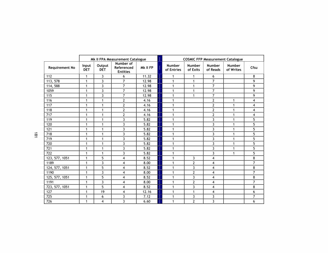
181

Mk II FPA Measurement Catalogue COSMIC FFP Measurement Catalogue

Requirement No Input DET

Output DET

Number of Referenced

Entities Mk II FP Number

of Entries Number of Exits

Number of Reads

Number of Writes Cfsu

112 1 3 6 11.32 1 1 6 8 113, 578 1 3 7 12.98 1 1 7 9 114, 588 1 3 7 12.98 1 1 7 9 1059 1 3 7 12.98 1 1 7 9 115 1 3 7 12.98 1 1 7 9 116 1 1 2 4.16 1 2 1 4 117 1 1 2 4.16 1 2 1 4 118 1 1 2 4.16 1 2 1 4 717 1 1 2 4.16 1 2 1 4 119 1 1 3 5.82 1 3 1 5 120 1 1 3 5.82 1 3 1 5 121 1 1 3 5.82 1 3 1 5 718 1 1 3 5.82 1 3 1 5 719 1 1 3 5.82 1 3 1 5 720 1 1 3 5.82 1 3 1 5 721 1 1 3 5.82 1 3 1 5 722 1 1 3 5.82 1 3 1 5 123, 577, 1051 1 5 4 8.52 1 3 4 8 1189 1 3 4 8.00 1 2 4 7 124, 577, 1051 1 5 4 8.52 1 3 4 8 1190 1 3 4 8.00 1 2 4 7 125, 577, 1051 1 5 4 8.52 1 3 4 8 1191 1 3 4 8.00 1 2 4 7 723, 577, 1051 1 5 4 8.52 1 3 4 8 127 1 19 4 12.16 1 1 4 6 725 1 6 3 7.12 1 3 3 7 726 1 4 3 6.60 1 2 3 6

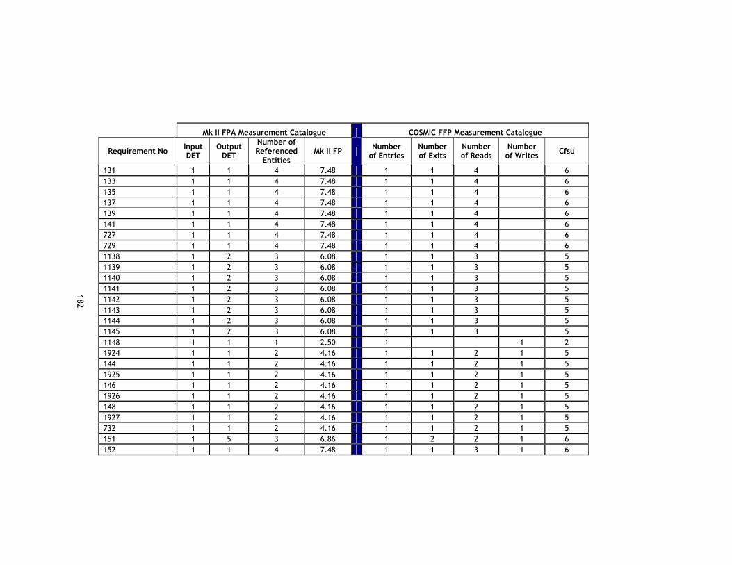
182

Mk II FPA Measurement Catalogue COSMIC FFP Measurement Catalogue

Requirement No Input DET

Output DET

Number of Referenced

Entities Mk II FP Number

of Entries Number of Exits

Number of Reads

Number of Writes Cfsu

131 1 1 4 7.48 1 1 4 6 133 1 1 4 7.48 1 1 4 6 135 1 1 4 7.48 1 1 4 6 137 1 1 4 7.48 1 1 4 6 139 1 1 4 7.48 1 1 4 6 141 1 1 4 7.48 1 1 4 6 727 1 1 4 7.48 1 1 4 6 729 1 1 4 7.48 1 1 4 6 1138 1 2 3 6.08 1 1 3 5 1139 1 2 3 6.08 1 1 3 5 1140 1 2 3 6.08 1 1 3 5 1141 1 2 3 6.08 1 1 3 5 1142 1 2 3 6.08 1 1 3 5 1143 1 2 3 6.08 1 1 3 5 1144 1 2 3 6.08 1 1 3 5 1145 1 2 3 6.08 1 1 3 5 1148 1 1 1 2.50 1 1 2 1924 1 1 2 4.16 1 1 2 1 5 144 1 1 2 4.16 1 1 2 1 5 1925 1 1 2 4.16 1 1 2 1 5 146 1 1 2 4.16 1 1 2 1 5 1926 1 1 2 4.16 1 1 2 1 5 148 1 1 2 4.16 1 1 2 1 5 1927 1 1 2 4.16 1 1 2 1 5 732 1 1 2 4.16 1 1 2 1 5 151 1 5 3 6.86 1 2 2 1 6 152 1 1 4 7.48 1 1 3 1 6

183

Mk II FPA Measurement Catalogue COSMIC FFP Measurement Catalogue

Requirement No Input DET

Output DET

Number of Referenced

Entities Mk II FP Number

of Entries Number of Exits

Number of Reads

Number of Writes Cfsu

153 1 1 4 7.48 1 1 3 1 6 154 1 1 4 7.48 1 1 3 1 6 155 1 1 4 7.48 1 1 3 1 6 156 1 4 4 8.26 1 1 4 6 157 1 4 4 8.26 1 1 4 6 736 1 3 4 8.00 1 1 4 6 737 1 3 4 8.00 1 1 4 6 1113 1 3 4 8.00 1 1 4 6 1114 1 3 4 8.00 1 1 4 6 1115 1 3 4 8.00 1 1 4 6 738 1 3 4 8.00 1 1 4 6 739 1 3 4 8.00 1 1 4 6 158 1 2 4 7.74 1 1 3 1 6 159 1 2 4 7.74 1 1 3 1 6 160 1 2 4 7.74 1 1 3 1 6 161 1 2 4 7.74 1 1 3 1 6 953, 59, 748 2 1 4 8.06 1 1 4 1 7 953, 58, 747 2 1 4 8.06 1 1 4 1 7 171, 172 2 1 4 8.06 1 1 4 1 7 175, 176 2 1 4 8.06 1 1 4 1 7 179, 180 2 1 4 8.06 1 1 4 1 7 183, 184 2 1 4 8.06 1 1 4 1 7 187, 188 2 1 4 8.06 1 1 4 1 7 191, 192 2 1 4 8.06 1 1 4 1 7 202, 205, 560, 561 2 1 4 8.06 1 1 4 1 7 203, 204 2 1 4 8.06 1 1 4 1 7 206, 209 2 1 4 8.06 1 1 4 1 7

184

Mk II FPA Measurement Catalogue COSMIC FFP Measurement Catalogue

Requirement No Input DET

Output DET

Number of Referenced

Entities Mk II FP Number

of Entries Number of Exits

Number of Reads

Number of Writes Cfsu

207, 208 2 1 4 8.06 1 1 4 1 7 211, 212 2 1 4 8.06 1 1 4 1 7 210, 213 2 1 4 8.06 1 1 4 1 7 214, 217 2 1 4 8.06 1 1 4 1 7 215, 216 2 1 4 8.06 1 1 4 1 7 750, 751 2 1 4 8.06 1 1 4 1 7 754, 755 2 1 4 8.06 1 1 4 1 7 758, 761, 562, 1042 2 1 4 8.06 1 1 4 1 7 759, 760 2 1 4 8.06 1 1 4 1 7 762, 765, 557 2 1 4 8.06 1 1 4 1 7 763, 764 2 1 4 8.06 1 1 4 1 7 900 1 9 3 7.90 1 8 3 12 779, 61 2 1 4 8.06 1 1 4 1 7 226, 227 2 1 4 8.06 1 1 4 1 7 786, 787 2 1 4 8.06 1 1 4 1 7 234, 235 2 1 4 8.06 1 1 4 1 7 238, 239 2 1 4 8.06 1 1 4 1 7 242 2 1 4 8.06 1 1 4 1 7 246, 247 2 1 4 8.06 1 1 4 1 7 250, 251 2 1 4 8.06 1 1 4 1 7 253, 256, 555, 556 2 1 4 8.06 1 1 4 1 7 254, 255 2 1 4 8.06 1 1 4 1 7 257, 260 2 1 4 8.06 1 1 4 1 7 258, 259 2 1 4 8.06 1 1 4 1 7 261, 264 2 1 4 8.06 1 1 4 1 7 262, 263 2 1 4 8.06 1 1 4 1 7

185

Mk II FPA Measurement Catalogue COSMIC FFP Measurement Catalogue

Requirement No Input DET

Output DET

Number of Referenced

Entities Mk II FP Number

of Entries Number of Exits

Number of Reads

Number of Writes Cfsu

265, 268 2 1 4 8.06 1 1 4 1 7 266, 267 2 1 4 8.06 1 1 4 1 7 790, 791 2 1 4 8.06 1 1 4 1 7 793, 796, 562, 1042 2 1 4 8.06 1 1 4 1 7 794, 795 2 1 4 8.06 1 1 4 1 7 806, 807 2 1 4 8.06 1 1 4 1 7 810, 811 2 1 4 8.06 1 1 4 1 7 814, 815 2 1 4 8.06 1 1 4 1 7 819, 745 2 1 4 8.06 1 1 4 1 7 276, 277 2 1 4 8.06 1 1 4 1 7 280, 281 2 1 4 8.06 1 1 4 1 7 284, 285 2 1 4 8.06 1 1 4 1 7 288, 289 2 1 4 8.06 1 1 4 1 7 292, 293 2 1 4 8.06 1 1 4 1 7 300, 301 2 1 4 8.06 1 1 4 1 7 304, 305 2 1 4 8.06 1 1 4 1 7 303, 306 2 1 4 8.06 1 1 4 1 7 308, 309 2 1 4 8.06 1 1 4 1 7 307, 310 2 1 4 8.06 1 1 4 1 7 311, 314 2 1 4 8.06 1 1 4 1 7 312, 313 2 1 4 8.06 1 1 4 1 7 316, 317 2 1 4 8.06 1 1 4 1 7 825, 826 2 1 4 8.06 1 1 4 1 7 829, 830 2 1 4 8.06 1 1 4 1 7 833, 834 2 1 4 8.06 1 1 4 1 7 837, 838 2 1 4 8.06 1 1 4 1 7

186

Mk II FPA Measurement Catalogue COSMIC FFP Measurement Catalogue

Requirement No Input DET

Output DET

Number of Referenced

Entities Mk II FP Number

of Entries Number of Exits

Number of Reads

Number of Writes Cfsu

841, 842 2 1 4 8.06 1 1 4 1 7 844, 847 2 1 4 8.06 1 1 4 1 7 845, 846 2 1 4 8.06 1 1 4 1 7 849, 850 2 1 4 8.06 1 1 4 1 7 853, 854 2 1 4 8.06 1 1 4 1 7 856, 859 2 1 4 8.06 1 1 4 1 7 857, 858 2 1 4 8.06 1 1 4 1 7 860, 863 2 1 4 8.06 1 1 4 1 7 861, 862 2 1 4 8.06 1 1 4 1 7 865, 866 2 1 4 8.06 1 1 4 1 7 869, 870 2 1 4 8.06 1 1 4 1 7 884 1 9 3 7.90 1 8 3 12 878, 63 2 1 4 8.06 1 1 4 1 7 879, 882 2 1 4 8.06 1 1 4 1 7 880, 881 2 1 4 8.06 1 1 4 1 7 1120, 1122 2 1 4 8.06 1 1 4 1 7 1121, 1123 2 1 4 8.06 1 1 4 1 7 1125, 1127 2 1 4 8.06 1 1 4 1 7 905, 907 2 1 4 8.06 1 1 4 1 7 911, 913 2 1 4 8.06 1 1 4 1 7 912, 914 2 1 4 8.06 1 1 4 1 7 1117, 1119 2 1 4 8.06 1 1 4 1 7 915, 917 2 1 4 8.06 1 1 4 1 7 916, 918 2 1 4 8.06 1 1 4 1 7 928, 930 2 1 4 8.06 1 1 4 1 7 929, 931 2 1 4 8.06 1 1 4 1 7 934, 936 2 1 4 8.06 1 1 4 1 7

187

Mk II FPA Measurement Catalogue COSMIC FFP Measurement Catalogue

Requirement No Input DET

Output DET

Number of Referenced

Entities Mk II FP Number

of Entries Number of Exits

Number of Reads

Number of Writes Cfsu

1940 1 31 5 16.94 1 1 5 7 90 1 31 5 16.94 1 1 5 7 321 1 16 2 8.06 1 12 2 15 941 13 10 2 13.46 13 10 2 25 942 13 10 2 13.46 13 10 2 25 943 13 10 2 13.46 13 10 2 25 333 1 2 3 6.08 1 2 3 6 334 1 2 3 6.08 1 2 3 6 322 1 3 4 8.00 1 1 4 6 323 1 3 4 8.00 1 1 4 6 324 1 3 4 8.00 1 1 4 6 325 1 3 4 8.00 1 1 4 6 326 1 3 4 8.00 1 1 4 6 327 1 3 4 8.00 1 1 4 6 328 1 3 4 8.00 1 1 4 6 329 1 3 4 8.00 1 1 4 6 330 1 3 4 8.00 1 1 4 6 335 1 1 2 4.16 1 1 2 1 5 372 1 5 4 8.52 1 3 4 8 373 1 5 4 8.52 1 3 4 8 341 1 8 4 9.30 1 3 4 8 342 1 9 4 9.56 1 3 4 8 343 1 8 4 9.30 1 2 4 7 344 1 13 4 10.60 1 4 4 9 1061 1 8 4 9.30 1 3 4 8 345 1 4 4 8.26 1 1 4 6 346 1 9 4 9.56 1 3 4 8

188

Mk II FPA Measurement Catalogue COSMIC FFP Measurement Catalogue

Requirement No Input DET

Output DET

Number of Referenced

Entities Mk II FP Number

of Entries Number of Exits

Number of Reads

Number of Writes Cfsu

1068 1 8 4 9.30 1 3 4 8 2113,..,2122, 2040, 2162, 378, 178, 181, 541, 549 2 15 11 23.32 1 3 11 1 16 2113,..,2122, 376, 2162, 378, 178, 181, 541, 549 2 15 11 23.32 1 3 11 1 16 2113,..,2122, 944, 2162, 378, 178, 181, 541, 549 2 15 11 23.32 1 3 11 1 16 2113,..,2122, 945, 2162, 378, 178, 181, 541, 549 2 15 11 23.32 1 3 11 1 16 383, 385,2123,.., 2126, 170, 173, 177, 174 2 13 10 21.14 1 4 10 15 946, 949, 2123,.., 2126, 170, 173, 177, 174 2 13 10 21.14 1 4 10 15 2131, 387, 749, 752, 545 2 8 9 18.18 1 2 9 12 2127, 406, 249, 252, 543 2 8 9 18.18 1 2 9 12 2128, 2130, 408, 249, 252, 544 2 8 9 18.18 1 2 9 12 2150, 411, 233, 236, 547 2 8 10 19.84 1 2 10 13 2150, 961, 233, 236, 547 2 8 10 19.84 1 2 10 13 2150, 413, 233, 236, 547 2 8 9 18.18 1 2 9 12

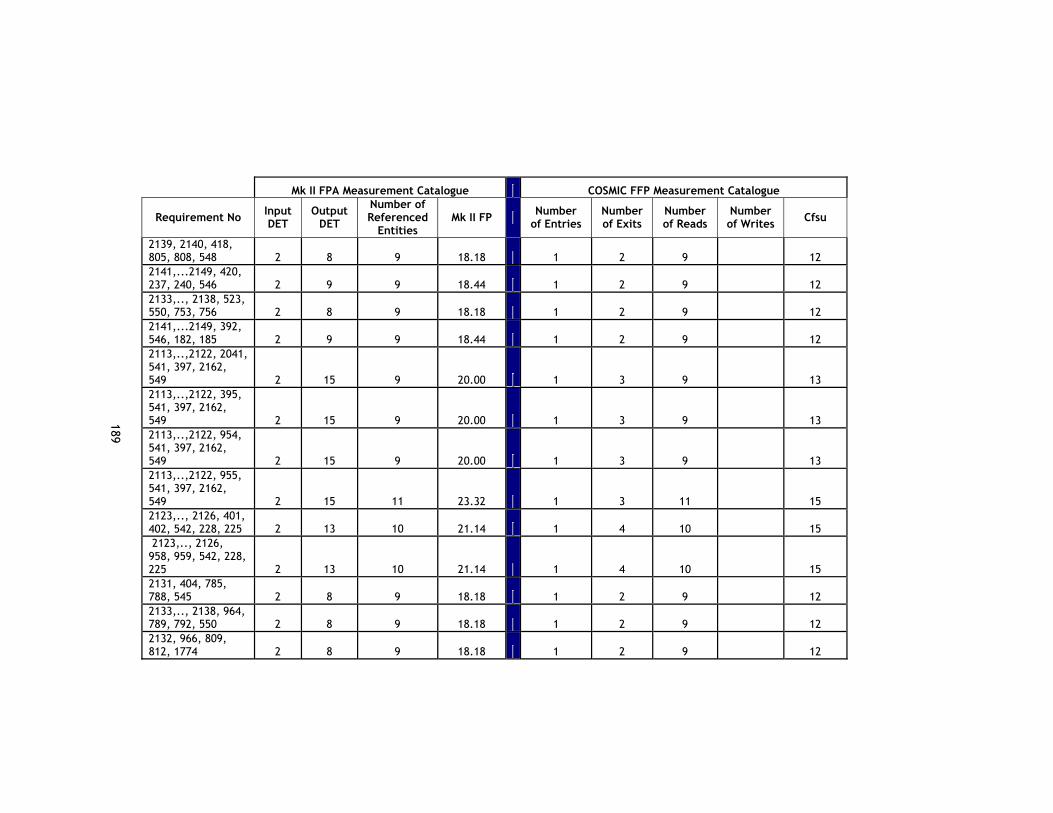
189

Mk II FPA Measurement Catalogue COSMIC FFP Measurement Catalogue

Requirement No Input DET

Output DET

Number of Referenced

Entities Mk II FP Number

of Entries Number of Exits

Number of Reads

Number of Writes Cfsu

2139, 2140, 418, 805, 808, 548 2 8 9 18.18 1 2 9 12 2141,...2149, 420, 237, 240, 546 2 9 9 18.44 1 2 9 12 2133,.., 2138, 523, 550, 753, 756 2 8 9 18.18 1 2 9 12 2141,...2149, 392, 546, 182, 185 2 9 9 18.44 1 2 9 12 2113,..,2122, 2041, 541, 397, 2162, 549 2 15 9 20.00 1 3 9 13 2113,..,2122, 395, 541, 397, 2162, 549 2 15 9 20.00 1 3 9 13 2113,..,2122, 954, 541, 397, 2162, 549 2 15 9 20.00 1 3 9 13 2113,..,2122, 955, 541, 397, 2162, 549 2 15 11 23.32 1 3 11 15 2123,.., 2126, 401, 402, 542, 228, 225 2 13 10 21.14 1 4 10 15 2123,.., 2126, 958, 959, 542, 228, 225 2 13 10 21.14 1 4 10 15 2131, 404, 785, 788, 545 2 8 9 18.18 1 2 9 12 2133,.., 2138, 964, 789, 792, 550 2 8 9 18.18 1 2 9 12 2132, 966, 809, 812, 1774 2 8 9 18.18 1 2 9 12

190

Mk II FPA Measurement Catalogue COSMIC FFP Measurement Catalogue

Requirement No Input DET

Output DET

Number of Referenced

Entities Mk II FP Number

of Entries Number of Exits

Number of Reads

Number of Writes Cfsu

965, 778, 60 2 2 7 13.30 1 2 7 10 424 1 10 3 8.16 1 1 3 5 2113,..,2122, 2042, 286, 283, 541, 428, 2162, 549 2 15 11 23.32 1 3 11 1 16 2113,..,2122,426, 286, 283, 541, 428, 2162, 549 2 15 11 23.32 1 3 11 1 16 2113,..,2122, 967, 286, 283, 541, 428, 2162, 549 2 15 11 23.32 1 3 11 1 16 2113,..,2122, 968, 286, 283, 541, 428, 2162, 549 2 15 11 23.32 1 3 11 1 16 2123,.., 2126, 432, 275, 278, 542, 433, 282, 279, 549 2 13 10 21.14 1 4 10 15 2123,.., 2126, 971, 275, 278, 542,, 972, 282, 279 2 13 10 21.14 1 4 10 15 2131, 435, 315, 318, 545 2 8 9 18.18 1 2 9 12 2127, 437, 827, 824, 543 2 8 9 18.18 1 2 9 12 2128, 2130, 441, 827, 824, 544 2 8 9 18.18 1 2 9 12 2150, 443, 290, 287, 547 2 8 10 19.84 1 2 10 13 2150, 974, 290, 287, 547 2 8 10 19.84 1 2 10 13 2150, 976, 290, 2 8 9 18.18 1 2 9 12

191

Mk II FPA Measurement Catalogue COSMIC FFP Measurement Catalogue

Requirement No Input DET

Output DET

Number of Referenced

Entities Mk II FP Number

of Entries Number of Exits

Number of Reads

Number of Writes Cfsu

287, 547 2139, 2140, 445, 848, 851, 548 2 8 9 18.18 1 2 9 12 2141,...2149, 980, 828, 831, 546 2 9 9 18.44 1 2 9 12 2132, 983, 852, 855, 1774 2 8 9 18.18 1 2 9 12 984, 818, 62 2 2 7 13.30 1 2 7 10 2133,.., 2138, 987, 832, 835, 550 2 8 9 18.18 1 2 9 12 2113,..,2122, 2043, 1122,1120, 541, 1131, 549, 2162 2 15 11 23.32 1 3 11 1 16 2113,..,2122, 1128, 1122,1120, 541, 1131, 549, 2162 2 15 11 23.32 1 3 11 1 16 2113,..,2122, 1129, 1122,1120, 541, 1131, 549, 2162 2 15 11 23.32 1 3 11 1 16 2113,..,2122, 1130, 1122,1120, 541, 1131, 549, 2162 2 15 11 23.32 1 3 11 1 16 2133,.., 2138, 1156, 904, 906, 550 2 8 9 18.18 1 2 9 12 1157, 877, 746 2 2 7 13.30 1 2 7 10 521 1 6 4 8.78 1 1 4 6 1011 1 3 1 3.02 1 1 1 3 1013 1 6 4 8.78 1 1 4 6 1012 1 3 1 3.02 1 1 1 3

192

Mk II FPA Measurement Catalogue COSMIC FFP Measurement Catalogue

Requirement No Input DET

Output DET

Number of Referenced

Entities Mk II FP Number

of Entries Number of Exits

Number of Reads

Number of Writes Cfsu

1135 1 6 4 8.78 1 1 4 6 1136 1 3 1 3.02 1 1 1 3 524.555.556 1 15 6 14.44 1 2 6 9 525 1 3 8 14.64 1 1 8 10 527 1 3 8 14.64 1 1 8 10 529 1 3 8 14.64 1 1 8 10 990 1 3 8 14.64 1 1 8 10 531 1 16 7 16.36 1 2 7 10 533 1 16 7 16.36 1 2 7 10 535, 253, 256, 555, 556 1 15 8 17.76 1 2 8 11 536 1 16 7 16.36 1 2 7 10 992 1 3 8 14.64 1 1 8 10 994, 813, 816, 557 1 3 8 14.64 1 1 8 10 996, 813, 816, 557 1 3 8 14.64 1 1 8 10 998, 813, 816, 557 1 3 8 14.64 1 1 8 10 1000, 299, 302, 555,556 1 15 8 17.76 1 2 8 11 1001, 864, 867, 557 1 3 9 16.30 1 1 9 11 1003, 864, 867, 557 1 3 9 16.30 1 1 9 11 1005, 864, 867, 557 1 3 9 16.30 1 1 9 11 1007, 864, 867, 557 1 3 9 16.30 1 1 9 11 1009, 836, 839, 560, 561 1 16 9 19.68 1 2 9 12 1010, 840, 843, 1 16 9 19.68 1 2 9 12

193

Mk II FPA Measurement Catalogue COSMIC FFP Measurement Catalogue

Requirement No Input DET

Output DET

Number of Referenced

Entities Mk II FP Number

of Entries Number of Exits

Number of Reads

Number of Writes Cfsu

562, 1042 1137, 1116, 1118, 555, 556 1 15 9 19.42 1 2 9 12 1099, 597 2 1 2 4.74 1 1 2 4 1100, 1192 2 1 2 4.74 1 1 2 4 1246 1 1 3 5.82 1 1 3 5 700 1 1 3 5.82 1 1 3 5 1247 1 1 3 5.82 1 1 3 5 7 1 1 3 5.82 1 1 3 5 1248 1 1 3 5.82 1 1 3 5 9 1 1 3 5.82 1 1 3 5 1291 1 1 3 5.82 1 1 3 5 1292 1 1 3 5.82 1 1 3 5 1293 1 1 3 5.82 1 1 3 5 1282 1 1 2 4.16 1 1 2 4 1283 1 3 1 3.02 1 2 1 4 1284 1 1 3 5.82 1 1 3 5 1285 1 1 3 5.82 1 1 3 5 1286 1 1 3 5.82 1 1 3 5 1287 1 1 3 5.82 1 1 3 5 46 1 1 3 5.82 1 1 3 5 1288 1 1 3 5.82 1 1 3 5 1289 1 1 3 5.82 1 1 3 5 1290 1 1 3 5.82 1 1 3 5 75 1 3 2 4.68 1 3 2 6 76 1 3 2 4.68 1 3 2 6 78 1 3 1 3.02 1 3 1 5

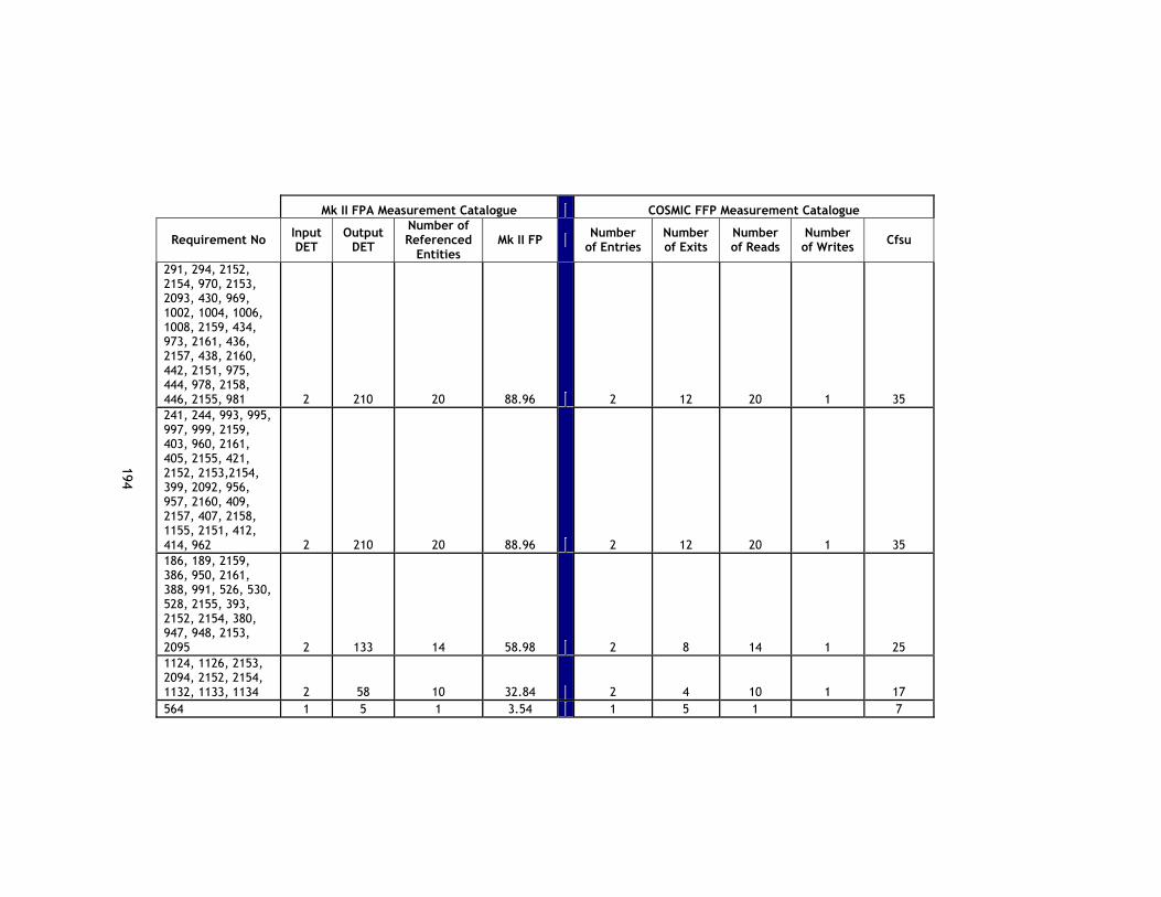
194

Mk II FPA Measurement Catalogue COSMIC FFP Measurement Catalogue

Requirement No Input DET

Output DET

Number of Referenced

Entities Mk II FP Number

of Entries Number of Exits

Number of Reads

Number of Writes Cfsu

291, 294, 2152, 2154, 970, 2153, 2093, 430, 969, 1002, 1004, 1006, 1008, 2159, 434, 973, 2161, 436, 2157, 438, 2160, 442, 2151, 975, 444, 978, 2158, 446, 2155, 981 2 210 20 88.96 2 12 20 1 35 241, 244, 993, 995, 997, 999, 2159, 403, 960, 2161, 405, 2155, 421, 2152, 2153,2154, 399, 2092, 956, 957, 2160, 409, 2157, 407, 2158, 1155, 2151, 412, 414, 962 2 210 20 88.96 2 12 20 1 35 186, 189, 2159, 386, 950, 2161, 388, 991, 526, 530, 528, 2155, 393, 2152, 2154, 380, 947, 948, 2153, 2095 2 133 14 58.98 2 8 14 1 25 1124, 1126, 2153, 2094, 2152, 2154, 1132, 1133, 1134 2 58 10 32.84 2 4 10 1 17 564 1 5 1 3.54 1 5 1 7

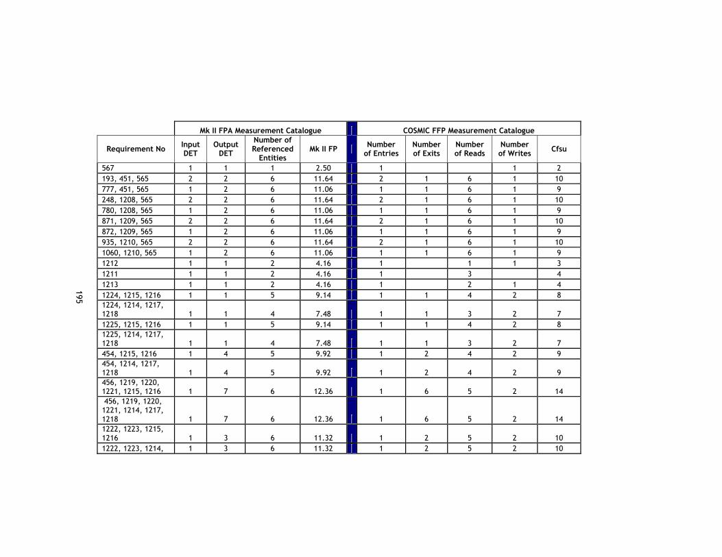
195

Mk II FPA Measurement Catalogue COSMIC FFP Measurement Catalogue

Requirement No Input DET

Output DET

Number of Referenced

Entities Mk II FP Number

of Entries Number of Exits

Number of Reads

Number of Writes Cfsu

567 1 1 1 2.50 1 1 2 193, 451, 565 2 2 6 11.64 2 1 6 1 10 777, 451, 565 1 2 6 11.06 1 1 6 1 9 248, 1208, 565 2 2 6 11.64 2 1 6 1 10 780, 1208, 565 1 2 6 11.06 1 1 6 1 9 871, 1209, 565 2 2 6 11.64 2 1 6 1 10 872, 1209, 565 1 2 6 11.06 1 1 6 1 9 935, 1210, 565 2 2 6 11.64 2 1 6 1 10 1060, 1210, 565 1 2 6 11.06 1 1 6 1 9 1212 1 1 2 4.16 1 1 1 3 1211 1 1 2 4.16 1 3 4 1213 1 1 2 4.16 1 2 1 4 1224, 1215, 1216 1 1 5 9.14 1 1 4 2 8 1224, 1214, 1217, 1218 1 1 4 7.48 1 1 3 2 7 1225, 1215, 1216 1 1 5 9.14 1 1 4 2 8 1225, 1214, 1217, 1218 1 1 4 7.48 1 1 3 2 7 454, 1215, 1216 1 4 5 9.92 1 2 4 2 9 454, 1214, 1217, 1218 1 4 5 9.92 1 2 4 2 9 456, 1219, 1220, 1221, 1215, 1216 1 7 6 12.36 1 6 5 2 14 456, 1219, 1220, 1221, 1214, 1217, 1218 1 7 6 12.36 1 6 5 2 14 1222, 1223, 1215, 1216 1 3 6 11.32 1 2 5 2 10 1222, 1223, 1214, 1 3 6 11.32 1 2 5 2 10

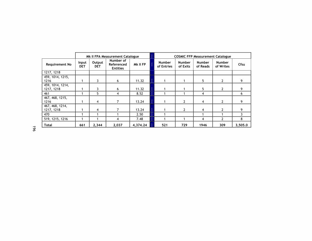
196

Mk II FPA Measurement Catalogue COSMIC FFP Measurement Catalogue

Requirement No Input DET

Output DET

Number of Referenced

Entities Mk II FP Number

of Entries Number of Exits

Number of Reads

Number of Writes Cfsu

1217, 1218 459, 1014, 1215, 1216 1 3 6 11.32 1 1 5 2 9 459, 1014, 1214, 1217, 1218 1 3 6 11.32 1 1 5 2 9 461 1 5 4 8.52 1 1 4 6 467, 468, 1215, 1216 1 4 7 13.24 1 2 4 2 9 467, 468, 1214, 1217, 1218 1 4 7 13.24 1 2 4 2 9 470 1 1 1 2.50 1 1 1 3 519, 1215, 1216 1 1 4 7.48 1 1 4 2 8

Total 661 2,344 2,037 4,374.24 521 729 1946 309 3,505.0

197

Case Study 2.1 - Subsystem B - Mk II FPA and COSMIC FFP Measurement Catalogue Requirement No Input

DET Output

DET Referenced Entity

Number Mk II FP Number of Entries

Number of Exits

Number of Reads

Number of Writes Cfsu

1640, 2170, 1632 3 5 6 13,00 1 1 6 8

2064, 2170, 1632 4 5 6 13,58 2 1 6 9

1641, 2169, 1632 3 5 6 13,00 1 1 6 8

2065, 2169, 1632 4 5 6 13,58 2 1 6 9

1642, 2167, 1632 3 5 6 13,00 1 1 6 8

2066, 2167, 1632 4 5 6 13,58 2 1 6 9

1643, 2168, 1632 3 5 6 13,00 1 1 6 8

2067, 2168, 1632 4 5 6 13,58 2 1 6 9

2068, 2170, 1632 3 5 6 13,00 1 1 6 8

2069, 2170, 1632 4 5 6 13,58 2 1 6 9

2070, 2169, 1632 3 5 6 13,00 1 1 6 8

2071, 2169, 1632 4 5 6 13,58 2 1 6 9

2072, 2167, 1632 3 5 6 13,00 1 1 6 8

2073, 2167, 1632 4 5 6 13,58 2 1 6 9

2074, 2168, 1632 3 5 6 13,00 1 1 6 8

2075, 2168, 1632 4 5 6 13,58 2 1 6 9

2076, 2170, 1632 3 5 6 13,00 1 1 6 8

2077, 2170, 1632 4 5 6 13,58 2 1 6 9

2078, 2169, 1632 3 5 6 13,00 1 1 6 8

2079, 2169, 1632 4 5 6 13,58 2 1 6 9

2080, 2167, 1632 3 5 6 13,00 1 1 6 8

2081, 2167, 1632 4 5 6 13,58 2 1 6 9

2082, 2168, 1632 3 5 6 13,00 1 1 6 8

2083, 2168, 1632 4 5 6 13,58 2 1 6 9

Case Study 2.1 - Subsystem B - M

k II FPA and CO

SMIC FFP M

easurement

Catalogue

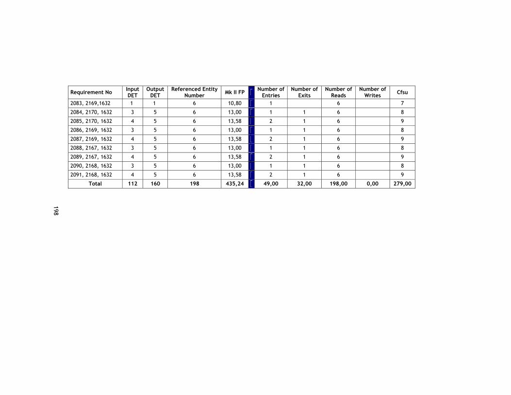
198

Requirement No Input DET

Output DET

Referenced Entity Number Mk II FP Number of

Entries Number of

Exits Number of

Reads Number of

Writes Cfsu

2083, 2169,1632 1 1 6 10,80 1 6 7

2084, 2170, 1632 3 5 6 13,00 1 1 6 8

2085, 2170, 1632 4 5 6 13,58 2 1 6 9

2086, 2169, 1632 3 5 6 13,00 1 1 6 8

2087, 2169, 1632 4 5 6 13,58 2 1 6 9

2088, 2167, 1632 3 5 6 13,00 1 1 6 8

2089, 2167, 1632 4 5 6 13,58 2 1 6 9

2090, 2168, 1632 3 5 6 13,00 1 1 6 8

2091, 2168, 1632 4 5 6 13,58 2 1 6 9

Total 112 160 198 435,24 49,00 32,00 198,00 0,00 279,00

199

Case Study 2.1 - Subsystem C - Mk II FPA and COSMIC FFP Measurement Catalogue

Requirement No Input DET

Output DET

Referenced Entity

Number Mk II FP Number of

Entries Number of

Exits Number of

Reads Number of

Writes Cfsu

2001, 1629, 1627 1 12 5 12 1 5 4 1 11

2001, 1630, 1627 1 12 5 12 1 5 4 1 11

2004, 1629, 1627 1 12 5 12 1 5 4 1 11

2004, 1630, 1627 1 12 5 12 1 5 4 1 11

2002, 1629, 1627 1 12 5 12 1 5 4 1 11

2002, 1630, 1627 1 12 5 12 1 5 4 1 11

2003, 1629, 1627 1 12 5 12 1 5 4 1 11

2003, 1630, 1627 1 12 5 12 1 5 4 1 11

1623 1 1 2 4.16 1 2 3

2021 1 1 3 5.82 1 3 4

1624 1 2 3 6.08 1 3 4

1627 1 11 1 5.1 1 1 2

1628 1 1 1 2.5 1 1 2

1629 1 1 2 4.16 1 2 3

1630 1 1 2 4.16 1 2 3

1609 1 1 3 5.82 1 3 4

2005 1 1 3 5.82 1 3 4

1610 1 1 3 5.82 1 3 4

2006 1 1 3 5.82 1 3 4

2007 1 1 3 5.82 1 3 4

1611 1 1 3 5.82 1 3 4

2008 1 1 3 5.82 1 3 4

2009 1 1 3 5.82 1 3 4

Case Study 2.1 - Subsystem C - M

k II FPA and CO

SMIC FFP M

easurement Catalogue

200

1338 1 1 3 5.82 1 3 4

2011 1 1 3 5.82 1 3 4

1339 1 1 3 5.82 1 3 4

2012 1 1 3 5.82 1 3 4

1337 1 1 4 7.48 1 4 5

2010 1 1 4 7.48 1 4 5

2010.1 1 1 1 2.5 1 1 2

2013 1 1 4 7.48 1 4 5

2014 1 1 4 7.48 1 4 5

2015 1 1 4 7.48 1 4 5

2016 1 1 4 7.48 1 4 5

2017 1 1 4 7.48 1 4 5

2018 1 1 4 7.48 1 4 5

2019 1 1 4 7.48 1 4 5

2020 1 1 4 7.48 1 4 5

1587 3 1 1 3.66 1 1 2

1615 3 5 5 11.34 1 5 6

1989 3 5 5 11.34 1 5 6

1991 1 2 7 12.72 1 7 8

1993 1 2 6 11.06 1 6 7

1992 1 2 7 12.72 1 7 8

1994 1 2 7 12.72 1 7 8

Total 51.00 156.00 169.00 350.68 45.00 40,00 159,00 8,00 252.00

201

Case Study 2.2 - Mk II FPA and COSMIC FFP Measurement Catalogue

Requirement No. Input DET

Output DET

Referenced Entity Number Mk II FP Number of

Entries Number of

Exits Number of

Reads Number of

Writes Cfsu

[000023] 1 1 1 2.50 1 1 1 3

[000024] 4 1 8 15.86 3 7 1 11

[000034] 1 1 1 2.50 1 1 1 3

[000035] 5 1 8 16.44 4 7 1 12

[000038] 1 1 1 2.50 1 1 1 3

[000039] 5 1 9 18.10 4 8 1 13

[000040] 0.00 0

[000041] 6 1 8 17.02 5 8 1 14

[000041_2] 2 1 1 3.08 1 1 1 3

[000042] 3 1 1 3.66 2 1 1 4

[000042_2] 6 1 8 17.02 5 8 1 14

[000043] 5 1 9 18.10 5 9 1 15

[000043_2] 2 1 2 4.74 1 2 1 4

[000044] 6 1 9 18.68 5 9 1 15 [000044_2] 3 1 2 5.32 2 2 1 5

[000045] 1 1 1 2.50 1 1 1 3

[000046] 2 1 1 3.08 1 1 1 3

[000047] 2 1 4 8.06 1 4 1 6

[000048] 1 1 1 2.50 1 1 2

[000049]_T1 2 1 2 4.74 1 2 1 4

T2 2 1 7 13.04 1 7 1 9

Case Study 2.2 - Mk II FPA

and COSM

IC FFP Measurem

ent Catalogue

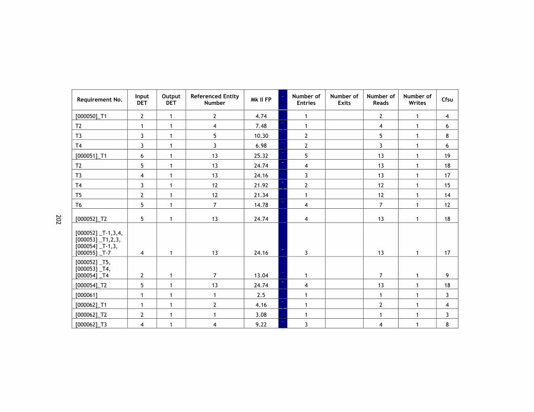
202

Requirement No. Input DET

Output DET

Referenced Entity Number Mk II FP Number of

Entries Number of

Exits Number of

Reads Number of

Writes Cfsu

[000050]_T1 2 1 2 4.74 1 2 1 4

T2 1 1 4 7.48 1 4 1 6

T3 3 1 5 10.30 2 5 1 8

T4 3 1 3 6.98 2 3 1 6

[000051]_T1 6 1 13 25.32 5 13 1 19

T2 5 1 13 24.74 4 13 1 18

T3 4 1 13 24.16 3 13 1 17

T4 3 1 12 21.92 2 12 1 15

T5 2 1 12 21.34 1 12 1 14

T6 5 1 7 14.78 4 7 1 12

[000052]_T2 5 1 13 24.74 4 13 1 18

[000052] _T-1,3,4, [000053] _T1,2,3, [000054] _T-1,3, [000055] _T-7 4 1 13 24.16 3 13 1 17

[000052] _T5, [000053] _T4, [000054] _T4 2 1 7 13.04 1 7 1 9

[000054]_T2 5 1 13 24.74 4 13 1 18

[000061] 1 1 1 2.5 1 1 1 3

[000062]_T1 1 1 2 4.16 1 2 1 4

[000062]_T2 2 1 1 3.08 1 1 1 3

[000062]_T3 4 1 4 9.22 3 4 1 8

203

Requirement No. Input DET

Output DET

Referenced Entity Number Mk II FP Number of

Entries Number of

Exits Number of

Reads Number of

Writes Cfsu

[000063] 4 1 4 9.22 3 4 1 8

[000064]_T2,T3, [000065]_T1,3,4,5, [000066]_T1,3,4,5, [000067]_1,3,4,5, [000068]_T1,3 4 1 4 9.22 3 4 1 8

[000064]_T1, [000065]_T2, [000066]_T2, [000067]_T2, [000068]_T2 3 1 2 5.32 2 2 1 5

[000072] 1 1 1 2.50 1 1 1 3

[000073] 5 1 4 9.80 4 4 1 9

[000074]_T1 3 1 4 8.64 2 4 1 7

T2 2 1 1 3.08 1 1 1 3

T3 2 1 1 3.08 1 1 1 3

[000076] 2 1 1 3.08 2 2

[000078] 1 1 1 2.50 1 1 1 3

[000079] 3 1 1 3.66 2 1 1 4

[000080] 0.00 0

[000080]_T2 2 1 1 3.08 1 1 1 3

[000081] 1 1 1 2.50 1 1 1 3

[000082] 3 1 2 5.32 2 2 1 5 [0000832] 2 1 1 3.08 1 1 1 3

204

Requirement No. Input DET

Output DET

Referenced Entity Number Mk II FP Number of

Entries Number of

Exits Number of

Reads Number of

Writes Cfsu

[000086] 2 1 1 3.08 1 1 1 3

[000088] 2 1 2 4.74 1 2 1 4

[000095] 1 1 1 2.50 1 1 1 3

[000096] 6 1 11 22.00 5 11 1 17

[000097] 2 1 2 4.74 1 2 1 4

[000098] 1 1 1 2.50 1 1 1 3

[000099] 1 1 3 5.82 1 3 1 5

[000100] 4 1 7 14.20 3 7 1 11

[000101] 4 1 8 15.86 3 8 1 12 [000101]_T2 4 1 8 15.86 3 8 1 12

[000106]_T1 1 1 1 2.50 1 1 1 3

T2 1 1 2 4.16 1 2 1 4

T3 1 1 1 2.50 1 1 1 3

[000108] 3 3 8 15.8 2 3 8 1 14

[000109] 3 3 9 17.46 2 3 9 1 15

[000110] 3 3 10 19.12 2 3 11 1 17

[000110]_T2 3 3 9 17.46 2 3 9 14

[000111]_T1 3 3 10 19.12 2 3 10 1 16

T2 1 1 3 5.82 1 3 1 5

[000112]_T1,2 1 1 5 9.14 1 5 1 7

T3 1 1 6 10.80 1 6 1 8

T4 1 1 5 9.14 1 5 1 7

[000114] 3 3 9 17.46 2 3 9 1 15

205

Requirement No. Input DET

Output DET

Referenced Entity Number Mk II FP Number of

Entries Number of

Exits Number of

Reads Number of

Writes Cfsu

[000115], [000116], [000117], [000118] 3 3 9 17.46 2 3 9 1 15

T2 3 3 10 19.12 2 3 10 1 16

[000119] 3 3 9 17.46 2 3 9 1 15

[000120], [000121], [000122], [000123] 3 3 9 17.46 2 3 9 1 15

[000124] 1 1 1 2.50 1 1 1 3

[000125] 0.00 0

[000125_T21] 1 1 2 4.16 1 2 1 4

[000125_T22] 3 1 11 20.26 2 11 1 14

[000126] 3 1 11 20.26 2 11 1 14

T2 3 1 10 18.60 2 10 1 13

[000131] 1 1 10 17.44 1 10 1 12

[000132] 1 1 10 17.44 1 10 1 12

T2 3 1 15 26.90 2 1 15 1 19

[000133] 3 1 15 26.90 2 1 15 1 19

T2 3 1 14 25.24 2 1 14 1 18

[000138] 1 1 1 2.50 1 1 1 3

[000139] 5 1 7 14.78 4 1 7 1 13

T2 7 1 6 14.28 6 1 6 1 14

T3 3 1 3 6.98 2 1 3 1 7

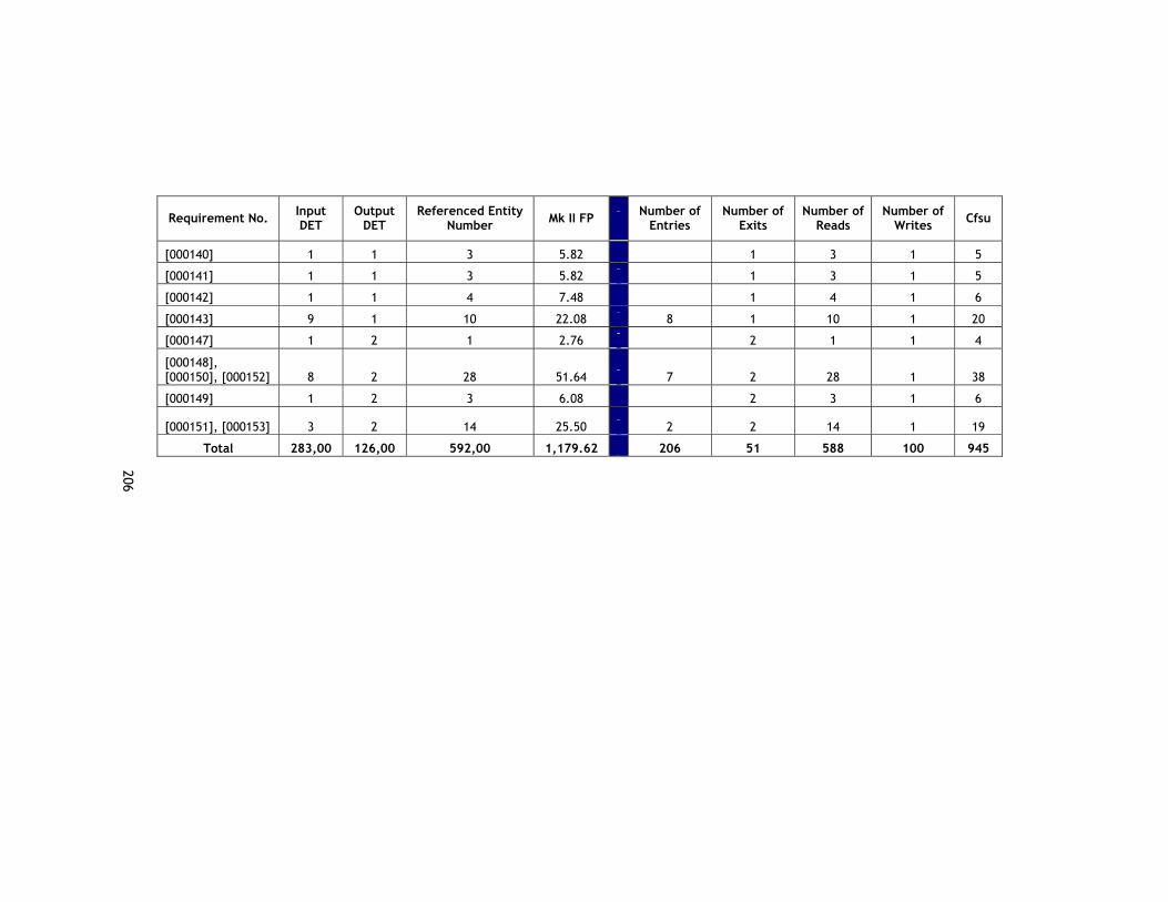
206

Requirement No. Input DET

Output DET

Referenced Entity Number Mk II FP Number of

Entries Number of

Exits Number of

Reads Number of

Writes Cfsu

[000140] 1 1 3 5.82 1 3 1 5

[000141] 1 1 3 5.82 1 3 1 5

[000142] 1 1 4 7.48 1 4 1 6

[000143] 9 1 10 22.08 8 1 10 1 20

[000147] 1 2 1 2.76 2 1 1 4

[000148], [000150], [000152] 8 2 28 51.64 7 2 28 1 38

[000149] 1 2 3 6.08 2 3 1 6

[000151], [000153] 3 2 14 25.50 2 2 14 1 19

Total 283,00 126,00 592,00 1,179.62 206 51 588 100 945

207

Case Study 2.3 - Mk II FPA and COSMIC FFP Measurement Catalogue Requirement

No Input DET

Output DET

Referenced Entity Number Mk II FP Number of

Entries Number of

Exits Number of

Reads Number of

Writes Cfsu

3.3.1.1.0, 3.3.1.1.5

1 35 7 21,30

1 8 7 16

3.3.1.1.1 31 36 7 38,96 5 8 7 5 25

3.3.1.1.2, 3.3.1.1.5

32 36 7 39,54

5 8 7 5 25

3.3.1.1.3 2 2 7 13,30 2 2 7 1 12

3.3.1.1.4, 3.3.1.1.5

2 36 7 22,14

2 8 7 1 18

3.3.1.1.6 1 1 10 17,44 1 5 5 11

3.3.1.2.2 6 10 1 7,74 1 2 1 1 5

3.3.1.3.1 10 10 1 10,06 1 2 1 1 5

3.3.1.3.2 8 10 1 8,90 1 2 1 1 5

3.3.1.3.3 2 11 1 5,68 2 3 1 1 7

3.3.1.4.1 12 13 1 12,00 1 2 1 1 5

3.3.1.4.2 13 13 1 12,58 1 2 1 1 5

3.3.1.4.3 2 14 1 6,46 2 3 1 1 7

3.3.1.5.1 0,00 0

T1 2 3 1 3,60 1 2 1 1 5

T2 2 3 1 3,60 1 2 1 1 5

T3 2 3 1 3,60 1 2 1 1 5

3.3.1.5.2 0,00 0

T1 2 3 1 3,60 1 2 1 1 5

Case Study 2.3 - Mk II FPA

and COSM

IC FFP Measurem

ent Catalogue

208

Requirement No

Input DET

Output DET

Referenced Entity Number Mk II FP Number of

Entries Number of

Exits Number of

Reads Number of

Writes Cfsu

T2 2 3 1 3,60 1 2 1 1 5

T3 2 3 1 3,60 1 2 1 1 5

3.3.1.5.3 0,00 0

T1 1 3 1 3,02 1 2 1 1 5

T2 1 3 1 3,02 1 2 1 1 5

T3 1 3 1 3,02 1 2 1 1 5

3.3.2.2.1 25 31 5 30,86 1 4 5 3 13

3.3.2.2.2 8 30 3 17,42 1 3 3 1 8

3.3.2.2.3 2 13 2 7,86 2 3 2 3 10

3.3.2.1.1- T1 2 30 3 13,94 1 3 3 7

T2 2 30 3 13,94 1 3 3 1 8

3.3.2.2.4.1 5 6 3 9,44 1 2 3 1 7

3.3.2.2.4.2 6 6 3 10,02 1 2 3 1 7

3.3.2.2.4.3 2 7 1 4,64 1 3 1 1 6

3.3.2.3.1 26 32 5 31,70 1 4 5 3 13

3.3.2.3.2 9 31 3 18,26 1 3 3 1 8

3.3.2.3.3 2 14 3 9,78 2 3 3 3 11

3.3.2.1.1-T1 2 31 2 12,54 1 3 2 6

T2 2 31 2 12,54 1 3 2 1 7

3.3.2.4.1 14 19 5 21,36 1 3 5 3 12

3.3.2.4.2 8 19 3 14,56 1 3 3 1 8

209

Requirement No

Input DET

Output DET

Referenced Entity Number Mk II FP Number of

Entries Number of

Exits Number of

Reads Number of

Writes Cfsu

3.3.2.4.3_T1 2 14 4 11,44 2 3 2 3 10

T2 2 19 2 9,42 1 3 2 6

T3 2 19 2 9,42 1 3 2 1 7

3.3.2.5.1 16 23 5 23,56 1 5 5 3 14

3.3.2.5.2 4 21 3 12,76 1 3 3 1 8

3.3.2.5.3_T1 2 20 3 11,34 2 4 3 2 11

T2 1 1 2 4,16 1 1 2 4

3.3.2.5.4 _T1 2 20 1 8,02 1 2 1 4

T2 1 1 1 2,50 1 1 2

T3 2 21 2 9,94 1 3 2 6

3.3.2.6.1, 3.3.1.2.1

19 25 5 25,82

1 5 5 2 13

3.3.2.6.2, 3.3.1.2.1

6 25 4 16,62

1 5 3 2 11

3.3.2.6.3, 3.3.1.2.1

2 10 2 7,08

2 3 2 3 10

T2 2 24 2 10,72 1 4 2 7

T3 2 24 2 10,72 1 4 2 1 8

3.3.2.7.1 16 22 7 26,62 3 6 7 5 21

3.3.2.7.2 8 21 5 18,40 3 5 5 4 17

3.3.2.7.3_T1 2 14 4 11,44 2 3 4 4 13

T2 2 21 3 11,60 1 5 3 9

T3 2 21 3 11,60 1 5 3 1 10

210

Requirement No

Input DET

Output DET

Referenced Entity Number Mk II FP Number of

Entries Number of

Exits Number of

Reads Number of

Writes Cfsu

3.3.2.8.1 1 22 6 16,26 1 5 4 2 12

3.3.2.8.2 2 15 3 10,04 2 4 3 2 11

3.3.2.8.3_T1 2 5 3 7,44 2 3 3 3 11

T2 2 15 3 10,04 1 4 3 8

T3 2 15 3 10,04 1 4 3 1 9

3.3.2.9.1 1 22 5 14,60 1 5 5 2 13

3.3.2.9.2 6 16 3 12,62 2 4 3 2 11

3.3.2.9.3_T1 2 5 3 7,44 2 3 3 3 11

T2 2 16 3 10,30 1 4 3 8

T3 2 16 3 10,30 1 4 3 1 9

3.3.2.10.1 11 18 7 22,68 2 5 7 4 18

3.3.2.10.2_T1 3 17 5 14,46 1 4 5 1 11

T2 2 17 4 12,22 2 4 4 3 13

T3 2 17 3 10,56 1 4 3 8

T4 2 15 3 10,04 1 4 3 1 9

3.3.2.11.1_T1 7 10 4 13,30 1 3 4 2 10

T2 2 13 2 7,86 1 3 2 6

T3 2 13 2 7,86 1 3 2 1 7

3.3.2.12.1_T1 1 6 3 7,12 1 1 3 5

T2 2 11 2 7,34 1 3 2 6

T3 2 11 2 7,34 1 3 2 1 7

211

Requirement No

Input DET

Output DET

Referenced Entity Number Mk II FP Number of

Entries Number of

Exits Number of

Reads Number of

Writes Cfsu

3.3.2.12.2_T1 1 6 3 7,12 1 1 3 5

T2 2 11 2 7,34 1 3 2 6

T3 2 11 2 7,34 1 3 2 1 7

3.3.2.12.3 0,00 0

3.3.2.12.4_T1 1 3 4 8,00 1 1 4 6

T2 2 8 2 6,56 1 3 2 6

T3 2 8 2 6,56 1 3 2 1 7

3.3.3.1.1 13 18 5 20,52 3 5 5 4 17

3.3.3.1.2 14 18 4 19,44 3 5 4 3 15

3.3.3.1.3_T1 3 14 4 12,02 2 5 4 2 13

T2 2 18 4 12,48 1 5 4 10

T3 2 18 4 12,48 1 5 4 1 11

3.3.3.2.1 14 19 3 18,04 1 3 3 2 9

3.3.3.2.2 15 19 2 16,96 1 3 2 1 7

3.3.3.2.3_T1 3 15 2 8,96 2 2 2 2 8

T2 2 19 2 9,42 1 3 2 6

T3 2 19 2 9,42 1 3 2 1 7

3.3.3.3.1 12 17 4 18,02 1 3 4 2 10

3.3.3.3.2 6 17 2 11,22 1 3 2 2 8

3.3.3.3.3_T1 3 13 3 10,10 2 2 2 3 9

T2 2 17 2 8,90 1 3 2 6

212

Requirement No

Input DET

Output DET

Referenced Entity Number Mk II FP Number of

Entries Number of

Exits Number of

Reads Number of

Writes Cfsu

T3 2 17 2 8,90 1 3 2 1 7

3.3.3.4.1 10 15 3 14,68 1 3 3 2 9

3.3.3.4.2 4 15 2 9,54 1 3 2 1 7

3.3.3.4.3_T1 3 11 2 7,92 2 2 2 2 8

T2 2 15 2 8,38 1 3 2 6

T3 2 15 2 8,38 1 3 2 1 7

3.3.3.5.1 9 14 3 13,84 1 3 3 2 9

3.3.3.5.2 5 14 2 9,86 1 3 2 1 7

3.3.3.5.3_T1 3 10 2 7,66 2 2 2 2 8

T2 2 14 2 8,12 1 3 2 6

T3 2 14 2 8,12 1 3 2 1 7

3.3.4.1 1 3 2 4,68 1 3 2 6

3.3.4.2_T1 1 3 3 6,34 1 3 3 7

T2 1 3 3 6,34 1 3 5 9

3.3.4.3 1 3 2 4,68 1 3 2 6

3.3.4.4_T1 1 3 3 6,34 1 3 3 7

T2 1 3 3 6,34 1 3 4 8

3.3.5_T1 0,00 0

T2 1 1 3 5,82 1 1 3 5

T3 1 1 1 2,50 1 1 2

Total 560,00 1,707,00 343,00 1,338,00 154,00 378,00 333,00 155,00 1,020,00

213

Case Study 3.1 - Subsystem A – ARCHI-DIM FSM measurement catalogue

INTERFACE Component Control PROCESS Component

Requirement No Number of Read DETs

(I/O Device)

Number of Write DETs (Volatile Storage)

Number of Read DETs (Volatile Storage)

Number of Write DETs (I/O Device)

INTERFACE Functional

Size (ADfsu)

Number of Read DETs (Volatile Storage)

Number of Write DETs (Volatile Storage)

Control PROCESS

Functional Size (ADfsu)

3 1 1 1 1 4 0 691 1 1 2 2 6 4 4 691_1 1 1 2 2 6 4 4 691_2 1 1 2 2 6 4 4 691_3 1 1 2 2 6 4 4 695, 108 1 1 6 6 14 4 4 4, 108, 696, 1200 1 1 18 18 38 1 5 6 1195, 1194, 1198, 5, 696, 1200

1 1 13 13 28 1 4 5

1196, 696, 1200 1 1 13 13 28 1 3 4 1199, 1200 1 1 6 6 14 2 3 5 6, 2055 1 1 4 4 10 1 1 1202, 2056 1 1 4 4 10 1 1 1203, 2057 1 1 4 4 10 1 1 1204, 2054 1 1 4 4 10 1 1 663 17 17 1 1 36 1 1 2 1280 17 17 1 1 36 1 1 2 1317 17 17 2 2 38 1 1 2 1205 1 1 2 1 1 2 1281 1 1 2 1 1 2 1588 2 2 4 1 1 2 31, 704,1260 5 5 10 3 1 4

Case Study 3.1 - Subsystem A

– ARCH

I-DIM

FSM M

easurement Catalogue

214

INTERFACE Component Control PROCESS Component

Requirement No Number of Read DETs

(I/O Device)

Number of Write DETs (Volatile Storage)

Number of Read DETs (Volatile Storage)

Number of Write DETs (I/O Device)

INTERFACE Functional

Size (ADfsu)

Number of Read DETs (Volatile Storage)

Number of Write DETs (Volatile Storage)

Control PROCESS

Functional Size (ADfsu)

33, 704,1260 5 5 10 3 1 4 35, 704,1260 5 5 10 3 1 4 681, 704,1260 5 5 10 3 1 4 671, 704,1260 1 1 2 2 1 3 673, 704,1260 1 1 2 2 1 3 675, 704,1260 1 1 2 2 1 3 678, 704,1260 1 1 2 2 1 3 1250 1 1 1 1 25, 698 1 1 1 1 4 1 1 27, 699 1 1 1 1 4 1 1 1941, 1747 1 1 1 1 4 1 1 29, 699 1 1 1 1 4 1 1 677, 697 1 1 1 1 4 1 1 1261, 697 1 1 1 1 4 1 1 711, 1633 1 1 1 1 4 1 1 714, 692 1 1 1 1 4 1 1 1942 1 1 1 1 4 1 1 713, 692 1 1 1 1 4 1 1 712, 1747 1 1 1 1 4 1 1 37, 1747 1 1 1 1 4 1 1 38, 1206 1 1 1 1 4 1 1 39, 1207 1 1 1 1 4 1 1 1943 1 1 1 1 4 1 1

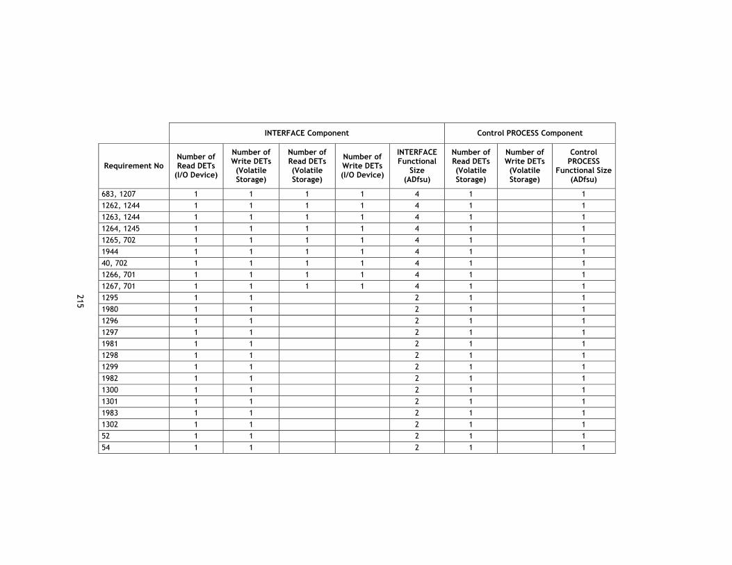
215

INTERFACE Component Control PROCESS Component

Requirement No Number of Read DETs

(I/O Device)

Number of Write DETs (Volatile Storage)

Number of Read DETs (Volatile Storage)

Number of Write DETs (I/O Device)

INTERFACE Functional

Size (ADfsu)

Number of Read DETs (Volatile Storage)

Number of Write DETs (Volatile Storage)

Control PROCESS

Functional Size (ADfsu)

683, 1207 1 1 1 1 4 1 1 1262, 1244 1 1 1 1 4 1 1 1263, 1244 1 1 1 1 4 1 1 1264, 1245 1 1 1 1 4 1 1 1265, 702 1 1 1 1 4 1 1 1944 1 1 1 1 4 1 1 40, 702 1 1 1 1 4 1 1 1266, 701 1 1 1 1 4 1 1 1267, 701 1 1 1 1 4 1 1 1295 1 1 2 1 1 1980 1 1 2 1 1 1296 1 1 2 1 1 1297 1 1 2 1 1 1981 1 1 2 1 1 1298 1 1 2 1 1 1299 1 1 2 1 1 1982 1 1 2 1 1 1300 1 1 2 1 1 1301 1 1 2 1 1 1983 1 1 2 1 1 1302 1 1 2 1 1 52 1 1 2 1 1 54 1 1 2 1 1

216

INTERFACE Component Control PROCESS Component

Requirement No Number of Read DETs

(I/O Device)

Number of Write DETs (Volatile Storage)

Number of Read DETs (Volatile Storage)

Number of Write DETs (I/O Device)

INTERFACE Functional

Size (ADfsu)

Number of Read DETs (Volatile Storage)

Number of Write DETs (Volatile Storage)

Control PROCESS

Functional Size (ADfsu)

56 1 1 2 1 1 689 1 1 2 1 1 1663 0 1 1 1318, 1251 1 1 1 1 4 2 1 3 1319, 664 1 1 1 1 4 2 1 3 1320, 15 1 1 1 1 4 2 1 3 1321,13 1 1 1 1 4 2 1 3 1322, 666 1 1 1 1 4 2 1 3 1323, 17 1 1 1 1 4 2 1 3 1324, 1252 1 1 1 1 4 2 1 3 1325, 19 1 1 1 1 4 2 1 3 75 3 3 6 2 2 76 3 3 6 2 2 78 3 3 6 2 2 892 1 1 8 8 18 1 1 80, 741 1 1 30 30 62 2 2 81, 741 1 1 15 15 32 2 2 742, 741 1 1 15 15 32 2 2 715, 741 1 1 15 15 32 2 2 165 1 1 2 1 1 2 167 1 1 2 1 1 2 92 1 1 2 3 1 4 1083 1 1 1 1 4 3 1 4

217

INTERFACE Component Control PROCESS Component

Requirement No Number of Read DETs

(I/O Device)

Number of Write DETs (Volatile Storage)

Number of Read DETs (Volatile Storage)

Number of Write DETs (I/O Device)

INTERFACE Functional

Size (ADfsu)

Number of Read DETs (Volatile Storage)

Number of Write DETs (Volatile Storage)

Control PROCESS

Functional Size (ADfsu)

1933 1 1 1 1 4 3 1 4 85, 87 1 1 3 3 8 2 2 4 85, 88 1 1 3 3 8 2 2 4 86, 696 1 1 7 7 16 2 2 4 740, 696 7 7 14 2 2 4 89, 2166, 2163 1 1 20 20 42 2 1 3 91, 87 1 1 3 3 8 1 2 3 91, 88 1 1 3 3 8 1 2 3 100 8 8 16 5 5 101 5 5 10 3 3 102 8 8 16 5 5 103 5 5 10 3 3 104 8 8 16 6 6 105 5 5 10 3 3 109, 583, 584 12 12 24 3 3 1152, 583, 584 7 7 14 3 3 112 3 3 6 1 1 113, 578 3 3 6 4 4 114, 588 3 3 6 4 4 1059 3 3 6 4 4 115 3 3 6 5 5 116 0 1 1 117 0 1 1

218

INTERFACE Component Control PROCESS Component

Requirement No Number of Read DETs

(I/O Device)

Number of Write DETs (Volatile Storage)

Number of Read DETs (Volatile Storage)

Number of Write DETs (I/O Device)

INTERFACE Functional

Size (ADfsu)

Number of Read DETs (Volatile Storage)

Number of Write DETs (Volatile Storage)

Control PROCESS

Functional Size (ADfsu)

118 0 1 1 717 0 1 1 119 0 2 2 120 0 2 2 121 0 2 2 718 0 2 2 719 0 2 2 720 0 2 2 721 0 2 2 722 0 2 2 123, 577, 1051 5 5 10 4 4 1189 3 3 6 2 2 124, 577, 1051 5 5 10 4 4 1190 3 3 6 2 2 125, 577, 1051 5 5 10 4 4 1191 3 3 6 2 2 723, 577, 1051 5 5 10 4 4 127 19 19 38 3 3 725 6 6 12 3 3 726 4 4 8 3 3 131 1 1 1 1 4 2 2 133 1 1 1 1 4 2 2 135 1 1 1 1 4 2 2

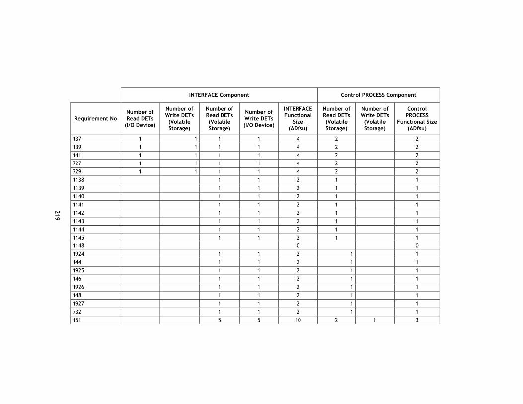
219

INTERFACE Component Control PROCESS Component

Requirement No Number of Read DETs

(I/O Device)

Number of Write DETs (Volatile Storage)

Number of Read DETs (Volatile Storage)

Number of Write DETs (I/O Device)

INTERFACE Functional

Size (ADfsu)

Number of Read DETs (Volatile Storage)

Number of Write DETs (Volatile Storage)

Control PROCESS

Functional Size (ADfsu)

137 1 1 1 1 4 2 2 139 1 1 1 1 4 2 2 141 1 1 1 1 4 2 2 727 1 1 1 1 4 2 2 729 1 1 1 1 4 2 2 1138 1 1 2 1 1 1139 1 1 2 1 1 1140 1 1 2 1 1 1141 1 1 2 1 1 1142 1 1 2 1 1 1143 1 1 2 1 1 1144 1 1 2 1 1 1145 1 1 2 1 1 1148 0 0 1924 1 1 2 1 1 144 1 1 2 1 1 1925 1 1 2 1 1 146 1 1 2 1 1 1926 1 1 2 1 1 148 1 1 2 1 1 1927 1 1 2 1 1 732 1 1 2 1 1 151 5 5 10 2 1 3

220

INTERFACE Component Control PROCESS Component

Requirement No Number of Read DETs

(I/O Device)

Number of Write DETs (Volatile Storage)

Number of Read DETs (Volatile Storage)

Number of Write DETs (I/O Device)

INTERFACE Functional

Size (ADfsu)

Number of Read DETs (Volatile Storage)

Number of Write DETs (Volatile Storage)

Control PROCESS

Functional Size (ADfsu)

152 1 1 1 1 4 2 1 3 153 1 1 1 1 4 2 1 3 154 1 1 1 1 4 2 1 3 155 1 1 1 1 4 2 1 3 156 3 4 7 2 2 157 3 4 7 2 2 736 3 3 6 2 2 737 3 3 6 2 2 1113 3 3 6 2 2 1114 3 3 6 2 2 1115 3 3 6 2 2 738 3 3 6 2 2 739 3 3 6 2 2 158 1 1 2 2 6 2 1 3 159 1 1 2 2 6 2 1 3 160 1 1 2 2 6 2 1 3 161 1 1 2 2 6 2 1 3 953, 59, 748 1 1 1 1 4 1 1 953, 58, 747 1 1 1 1 4 1 1 171, 172 1 1 1 1 4 1 1 175, 176 1 1 1 1 4 1 1 179, 180 1 1 1 1 4 1 1 183, 184 1 1 1 1 4 1 1

221

INTERFACE Component Control PROCESS Component

Requirement No Number of Read DETs

(I/O Device)

Number of Write DETs (Volatile Storage)

Number of Read DETs (Volatile Storage)

Number of Write DETs (I/O Device)

INTERFACE Functional

Size (ADfsu)

Number of Read DETs (Volatile Storage)

Number of Write DETs (Volatile Storage)

Control PROCESS

Functional Size (ADfsu)

187, 188 1 1 1 1 4 1 1 191, 192 1 1 1 1 4 1 1 202, 205, 560, 561 1 1 1 1 4 1 1

203, 204 1 1 1 1 4 1 1 206, 209 1 1 1 1 4 1 1 207, 208 1 1 1 1 4 1 1 211, 212 1 1 1 1 4 1 1 210, 213 1 1 1 1 4 1 1 214, 217 1 1 1 1 4 1 1 215, 216 1 1 1 1 4 1 1 750, 751 1 1 1 1 4 1 1 754, 755 1 1 1 1 4 1 1 758, 761, 562, 1042 1 1 1 1 4 1 1

759, 760 1 1 1 1 4 1 1 762, 765, 557 1 1 1 1 4 1 1 763, 764 1 1 1 1 4 1 1 900 1 1 8 8 18 1 1 779, 61 1 1 1 1 4 1 1 226, 227 1 1 1 1 4 1 1 786, 787 1 1 1 1 4 1 1 234, 235 1 1 1 1 4 1 1 238, 239 1 1 1 1 4 1 1

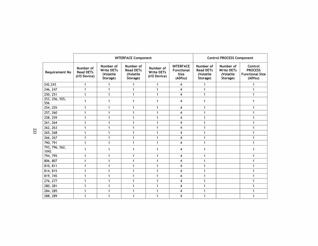
222

INTERFACE Component Control PROCESS Component

Requirement No Number of Read DETs

(I/O Device)

Number of Write DETs (Volatile Storage)

Number of Read DETs (Volatile Storage)

Number of Write DETs (I/O Device)

INTERFACE Functional

Size (ADfsu)

Number of Read DETs (Volatile Storage)

Number of Write DETs (Volatile Storage)

Control PROCESS

Functional Size (ADfsu)

242.243 1 1 1 1 4 1 1 246, 247 1 1 1 1 4 1 1 250, 251 1 1 1 1 4 1 1 253, 256, 555, 556 1 1 1 1 4 1 1

254, 255 1 1 1 1 4 1 1 257, 260 1 1 1 1 4 1 1 258, 259 1 1 1 1 4 1 1 261, 264 1 1 1 1 4 1 1 262, 263 1 1 1 1 4 1 1 265, 268 1 1 1 1 4 1 1 266, 267 1 1 1 1 4 1 1 790, 791 1 1 1 1 4 1 1 793, 796, 562, 1042 1 1 1 1 4 1 1

794, 795 1 1 1 1 4 1 1 806, 807 1 1 1 1 4 1 1 810, 811 1 1 1 1 4 1 1 814, 815 1 1 1 1 4 1 1 819, 745 1 1 1 1 4 1 1 276, 277 1 1 1 1 4 1 1 280, 281 1 1 1 1 4 1 1 284, 285 1 1 1 1 4 1 1 288, 289 1 1 1 1 4 1 1

223

INTERFACE Component Control PROCESS Component

Requirement No Number of Read DETs

(I/O Device)

Number of Write DETs (Volatile Storage)

Number of Read DETs (Volatile Storage)

Number of Write DETs (I/O Device)

INTERFACE Functional

Size (ADfsu)

Number of Read DETs (Volatile Storage)

Number of Write DETs (Volatile Storage)

Control PROCESS

Functional Size (ADfsu)

292, 293 1 1 1 1 4 1 1 300, 301 1 1 1 1 4 1 1 304, 305 1 1 1 1 4 1 1 303, 306 1 1 1 1 4 1 1 308, 309 1 1 1 1 4 1 1 307, 310 1 1 1 1 4 1 1 311, 314 1 1 1 1 4 1 1 312, 313 1 1 1 1 4 1 1 316, 317 1 1 1 1 4 1 1 825, 826 1 1 1 1 4 1 1 829, 830 1 1 1 1 4 1 1 833, 834 1 1 1 1 4 1 1 837, 838 1 1 1 1 4 1 1 841, 842 1 1 1 1 4 1 1 844, 847 1 1 1 1 4 1 1 845, 846 1 1 1 1 4 1 1 849, 850 1 1 1 1 4 1 1 853, 854 1 1 1 1 4 1 1 856, 859 1 1 1 1 4 1 1 857, 858 1 1 1 1 4 1 1 860, 863 1 1 1 1 4 1 1 861, 862 1 1 1 1 4 1 1 865, 866 1 1 1 1 4 1 1

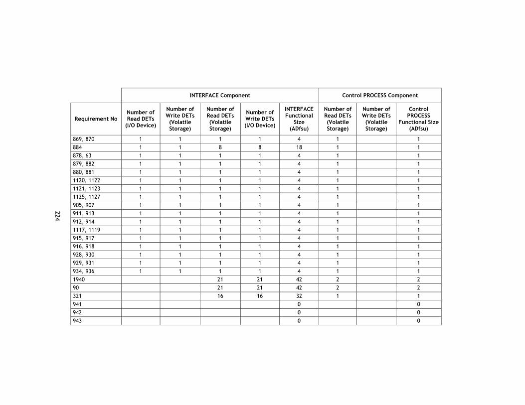
224

INTERFACE Component Control PROCESS Component

Requirement No Number of Read DETs

(I/O Device)

Number of Write DETs (Volatile Storage)

Number of Read DETs (Volatile Storage)

Number of Write DETs (I/O Device)

INTERFACE Functional

Size (ADfsu)

Number of Read DETs (Volatile Storage)

Number of Write DETs (Volatile Storage)

Control PROCESS

Functional Size (ADfsu)

869, 870 1 1 1 1 4 1 1 884 1 1 8 8 18 1 1 878, 63 1 1 1 1 4 1 1 879, 882 1 1 1 1 4 1 1 880, 881 1 1 1 1 4 1 1 1120, 1122 1 1 1 1 4 1 1 1121, 1123 1 1 1 1 4 1 1 1125, 1127 1 1 1 1 4 1 1 905, 907 1 1 1 1 4 1 1 911, 913 1 1 1 1 4 1 1 912, 914 1 1 1 1 4 1 1 1117, 1119 1 1 1 1 4 1 1 915, 917 1 1 1 1 4 1 1 916, 918 1 1 1 1 4 1 1 928, 930 1 1 1 1 4 1 1 929, 931 1 1 1 1 4 1 1 934, 936 1 1 1 1 4 1 1 1940 21 21 42 2 2 90 21 21 42 2 2 321 16 16 32 1 1 941 0 0 942 0 0 943 0 0

225

INTERFACE Component Control PROCESS Component

Requirement No Number of Read DETs

(I/O Device)

Number of Write DETs (Volatile Storage)

Number of Read DETs (Volatile Storage)

Number of Write DETs (I/O Device)

INTERFACE Functional

Size (ADfsu)

Number of Read DETs (Volatile Storage)

Number of Write DETs (Volatile Storage)

Control PROCESS

Functional Size (ADfsu)

333 1 1 2 2 6 2 2 334 1 1 2 2 6 2 2 322 3 3 6 4 4 323 3 3 6 4 4 324 3 3 6 4 4 325 3 3 6 4 4 326 3 3 6 4 4 327 3 3 6 4 4 328 3 3 6 4 4 329 3 3 6 4 4 330 3 3 6 4 4 335 1 1 2 2 1 3 372 5 5 10 8 8 373 5 5 10 8 8 341 7 7 14 10 10 342 9 9 18 12 12 343 8 8 16 11 11 344 13 13 26 16 16 1061 8 8 16 11 11 345 4 4 8 7 7 346 9 9 18 12 12 1068 8 8 16 11 11

226

INTERFACE Component Control PROCESS Component

Requirement No Number of Read DETs

(I/O Device)

Number of Write DETs (Volatile Storage)

Number of Read DETs (Volatile Storage)

Number of Write DETs (I/O Device)

INTERFACE Functional

Size (ADfsu)

Number of Read DETs (Volatile Storage)

Number of Write DETs (Volatile Storage)

Control PROCESS

Functional Size (ADfsu)

2113,..,2122, 2040, 2162, 378, 178, 181, 541, 549

2 2 15 15 34 2 2

2113,..,2122, 376, 2162, 378, 178, 181, 541, 549

2 2 15 15 34 2 2

2113,..,2122, 944, 2162, 378, 178, 181, 541, 549

2 2 15 15 34 2 2

2113,..,2122, 945, 2162, 378, 178, 181, 541, 549

2 2 15 15 34 2 2

383, 385,2123,.., 2126, 170, 173, 177, 174

2 2 13 13 30 2 2

946, 949, 2123,.., 2126, 170, 173, 177, 174

2 2 13 13 30 2 2

2131, 387, 749, 752, 545 2 2 8 8 20 2 2

2127, 406, 249, 252, 543 2 2 8 8 20 2 2

2128, 2130, 408, 249, 252, 544 2 2 8 8 20 2 2

2150, 411, 233, 2 2 8 8 20 3 3

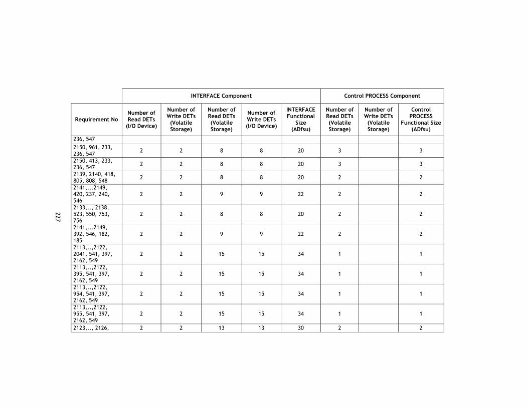
227

INTERFACE Component Control PROCESS Component

Requirement No Number of Read DETs

(I/O Device)

Number of Write DETs (Volatile Storage)

Number of Read DETs (Volatile Storage)

Number of Write DETs (I/O Device)

INTERFACE Functional

Size (ADfsu)

Number of Read DETs (Volatile Storage)

Number of Write DETs (Volatile Storage)

Control PROCESS

Functional Size (ADfsu)

236, 547 2150, 961, 233, 236, 547 2 2 8 8 20 3 3

2150, 413, 233, 236, 547 2 2 8 8 20 3 3

2139, 2140, 418, 805, 808, 548 2 2 8 8 20 2 2

2141,...2149, 420, 237, 240, 546

2 2 9 9 22 2 2

2133,.., 2138, 523, 550, 753, 756

2 2 8 8 20 2 2

2141,...2149, 392, 546, 182, 185

2 2 9 9 22 2 2

2113,..,2122, 2041, 541, 397, 2162, 549

2 2 15 15 34 1 1

2113,..,2122, 395, 541, 397, 2162, 549

2 2 15 15 34 1 1

2113,..,2122, 954, 541, 397, 2162, 549

2 2 15 15 34 1 1

2113,..,2122, 955, 541, 397, 2162, 549

2 2 15 15 34 1 1

2123,.., 2126, 2 2 13 13 30 2 2

228

INTERFACE Component Control PROCESS Component

Requirement No Number of Read DETs

(I/O Device)

Number of Write DETs (Volatile Storage)

Number of Read DETs (Volatile Storage)

Number of Write DETs (I/O Device)

INTERFACE Functional

Size (ADfsu)

Number of Read DETs (Volatile Storage)

Number of Write DETs (Volatile Storage)

Control PROCESS

Functional Size (ADfsu)

401, 402, 542, 228, 225 2123,.., 2126, 958, 959, 542, 228, 225

2 2 13 13 30 2 2

2131, 404, 785, 788, 545 2 2 8 8 20 2 2

2133,.., 2138, 964, 789, 792, 550

2 2 8 8 20 2 2

2132, 966, 809, 812, 1774 2 2 8 8 20 2 2

965, 778, 60 2 2 2 2 8 2 2 424 10 10 20 9 9 2113,..,2122, 2042, 286, 283, 541, 428, 2162, 549

2 2 15 15 34 2 2

2113,..,2122,426, 286, 283, 541, 428, 2162, 549

2 2 15 15 34 2 2

2113,..,2122, 967, 286, 283, 541, 428, 2162, 549

2 2 15 15 34 2 2

2113,..,2122, 968, 286, 283, 541, 428, 2162, 549

2 2 15 15 34 2 2

229

INTERFACE Component Control PROCESS Component

Requirement No Number of Read DETs

(I/O Device)

Number of Write DETs (Volatile Storage)

Number of Read DETs (Volatile Storage)

Number of Write DETs (I/O Device)

INTERFACE Functional

Size (ADfsu)

Number of Read DETs (Volatile Storage)

Number of Write DETs (Volatile Storage)

Control PROCESS

Functional Size (ADfsu)

2123,.., 2126, 432, 275, 278, 542, 433, 282, 279, 549

2 2 13 13 30 2 2

2123,.., 2126, 971, 275, 278, 542,, 972, 282, 279

2 2 13 13 30 2 2

2131, 435, 315, 318, 545 2 2 8 8 20 2 2

2127, 437, 827, 824, 543 2 2 8 8 20 2 2

2128, 2130, 441, 827, 824, 544 2 2 8 8 20 2 2

2150, 443, 290, 287, 547 2 2 8 8 20 3 3

2150, 974, 290, 287, 547 2 2 8 8 20 3 3

2150, 976, 290, 287, 547 2 2 8 8 20 3 3

2139, 2140, 445, 848, 851, 548 2 2 8 8 20 2 2

2141,...2149, 980, 828, 831, 546

2 2 9 9 22 2 2

2132, 983, 852, 855, 1774 2 2 8 8 20 2 2

984, 818, 62 2 2 2 2 8 2 2 2133,.., 2138, 2 2 8 8 20 2 2

230

INTERFACE Component Control PROCESS Component

Requirement No Number of Read DETs

(I/O Device)

Number of Write DETs (Volatile Storage)

Number of Read DETs (Volatile Storage)

Number of Write DETs (I/O Device)

INTERFACE Functional

Size (ADfsu)

Number of Read DETs (Volatile Storage)

Number of Write DETs (Volatile Storage)

Control PROCESS

Functional Size (ADfsu)

987, 832, 835, 550 2113,..,2122, 2043, 1122,1120, 541, 1131, 549, 2162

2 2 15 15 34 2 2

2113,..,2122, 1128, 1122,1120, 541, 1131, 549, 2162

2 2 15 15 34 2 2

2113,..,2122, 1129, 1122,1120, 541, 1131, 549, 2162

2 2 15 15 34 2 2

2113,..,2122, 1130, 1122,1120, 541, 1131, 549, 2162

2 2 15 15 34 2 2

2133,.., 2138, 1156, 904, 906, 550

2 2 8 8 20 2 2

1157, 877, 746 2 2 2 2 8 2 2 521 6 6 12 1 1 1011 3 3 6 1 1 1013 6 6 12 1 1 1012 3 3 6 1 1 1135 6 6 12 1 1

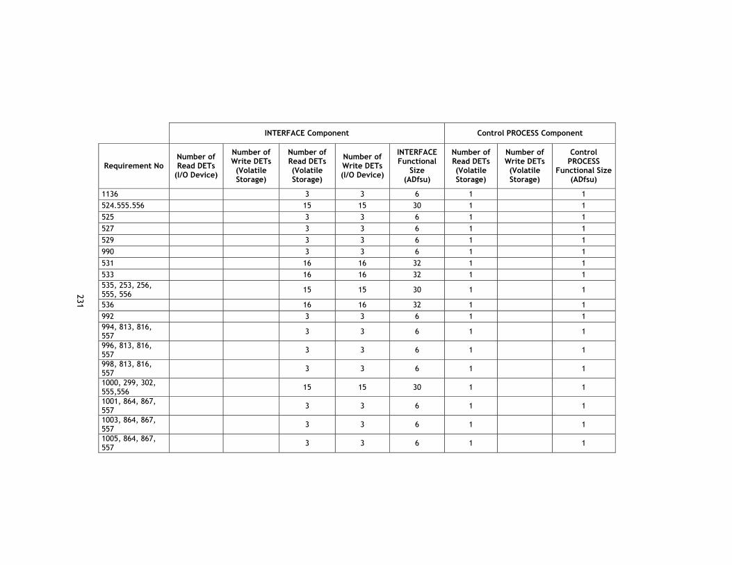
231

INTERFACE Component Control PROCESS Component

Requirement No Number of Read DETs

(I/O Device)

Number of Write DETs (Volatile Storage)

Number of Read DETs (Volatile Storage)

Number of Write DETs (I/O Device)

INTERFACE Functional

Size (ADfsu)

Number of Read DETs (Volatile Storage)

Number of Write DETs (Volatile Storage)

Control PROCESS

Functional Size (ADfsu)

1136 3 3 6 1 1 524.555.556 15 15 30 1 1 525 3 3 6 1 1 527 3 3 6 1 1 529 3 3 6 1 1 990 3 3 6 1 1 531 16 16 32 1 1 533 16 16 32 1 1 535, 253, 256, 555, 556 15 15 30 1 1

536 16 16 32 1 1 992 3 3 6 1 1 994, 813, 816, 557 3 3 6 1 1

996, 813, 816, 557 3 3 6 1 1

998, 813, 816, 557 3 3 6 1 1

1000, 299, 302, 555,556 15 15 30 1 1

1001, 864, 867, 557 3 3 6 1 1

1003, 864, 867, 557 3 3 6 1 1

1005, 864, 867, 557 3 3 6 1 1

232

INTERFACE Component Control PROCESS Component

Requirement No Number of Read DETs

(I/O Device)

Number of Write DETs (Volatile Storage)

Number of Read DETs (Volatile Storage)

Number of Write DETs (I/O Device)

INTERFACE Functional

Size (ADfsu)

Number of Read DETs (Volatile Storage)

Number of Write DETs (Volatile Storage)

Control PROCESS

Functional Size (ADfsu)

1007, 864, 867, 557 3 3 6 1 1

1009, 836, 839, 560, 561 16 16 32 2 2

1010, 840, 843, 562, 1042 16 16 32 2 2

1137, 1116, 1118, 555, 556 15 15 30 2 2

1099, 597 1 1 1 1 4 1 1 1100, 1192 1 1 1 1 4 1 1 1246 1 1 2 1 1 700 1 1 2 1 1 1247 1 1 2 1 1 7 1 1 2 1 1 1248 1 1 2 1 1 9 1 1 2 1 1 1291 1 1 2 1 1 1292 1 1 2 1 1 1293 1 1 2 1 1 1282 1 1 1 1 4 2 2 1283 2 2 4 1 1 1284 1 1 2 1 1 1285 1 1 2 1 1 1286 1 1 2 1 1 1287 1 1 2 1 1

233

INTERFACE Component Control PROCESS Component

Requirement No Number of Read DETs

(I/O Device)

Number of Write DETs (Volatile Storage)

Number of Read DETs (Volatile Storage)

Number of Write DETs (I/O Device)

INTERFACE Functional

Size (ADfsu)

Number of Read DETs (Volatile Storage)

Number of Write DETs (Volatile Storage)

Control PROCESS

Functional Size (ADfsu)

46 1 1 2 1 1 1288 1 1 2 1 1 1289 1 1 2 1 1 1290 1 1 2 1 1 75 3 3 6 2 2 76 3 3 6 2 2 78 3 3 6 1 1 CUSTOM -291, 294, 2152, 2154, 970, 2153, 2093, 430, 969, 1002, 1004, 1006, 1008, 2159, 434, 973, 2161, 436, 2157, 438, 2160, 442, 2151, 975, 444, 978, 2158, 446, 2155, 981

2 2 210 210 424 3 3

IFR-241, 244, 993, 995, 997, 999, 2159, 403, 960, 2161, 405, 2155, 421, 2152, 2153,2154, 399, 2092, 956, 957, 2160, 409, 2157, 407, 2158, 1155, 2151, 412, 414,

2 2 210 210 424 3 3

234

INTERFACE Component Control PROCESS Component

Requirement No Number of Read DETs

(I/O Device)

Number of Write DETs (Volatile Storage)

Number of Read DETs (Volatile Storage)

Number of Write DETs (I/O Device)

INTERFACE Functional

Size (ADfsu)

Number of Read DETs (Volatile Storage)

Number of Write DETs (Volatile Storage)

Control PROCESS

Functional Size (ADfsu)

962

VFR-186, 189, 2159, 386, 950, 2161, 388, 991, 526, 530, 528, 2155, 393, 2152, 2154, 380, 947, 948, 2153, 2095

2 2 133 133 270 2 2

WSI - 1124, 1126, 2153, 2094, 2152, 2154, 1132, 1133, 1134

2 2 58 58 120 2 2

564 0 0 567 0 0 193, 451, 565 2 2 2 2 8 4 1 5 777, 451, 565 2 2 4 4 1 5 248, 1208, 565 2 2 2 2 8 4 1 5 780, 1208, 565 2 2 4 4 1 5 871, 1209, 565 2 2 2 2 8 4 1 5 872, 1209, 565 2 2 4 4 1 5 935, 1210, 565 2 2 2 2 8 4 1 5 1060, 1210, 565 2 2 4 4 1 5

235

INTERFACE Component Control PROCESS Component

Requirement No Number of Read DETs

(I/O Device)

Number of Write DETs (Volatile Storage)

Number of Read DETs (Volatile Storage)

Number of Write DETs (I/O Device)

INTERFACE Functional

Size (ADfsu)

Number of Read DETs (Volatile Storage)

Number of Write DETs (Volatile Storage)

Control PROCESS

Functional Size (ADfsu)

1212 0 1 1 2 1211 1 1 2 3 3 1213 0 3 1 4 1224, 1215, 1216 1 1 2 6 2 8 1224, 1214, 1217, 1218 1 1 2 6 2 8

1225, 1215, 1216 1 1 2 6 2 8 1225, 1214, 1217, 1218 1 1 2 6 2 8

454, 1215, 1216 4 4 8 5 2 7 454, 1214, 1217, 1218 4 4 8 7 2 9

456, 1219, 1220, 1221, 1215, 1216 7 7 14 8 2 10

456, 1219, 1220, 1221, 1214, 1217, 1218

7 7 14 8 2 10

1222, 1223, 1215, 1216 3 3 6 7 2 9

1222, 1223, 1214, 1217, 1218 3 3 6 10 2 12

459, 1014, 1215, 1216 3 3 6 7 2 9

459, 1014, 1214, 1217, 1218 3 3 6 8 2 10

461 5 5 10 4 4 467, 468, 1215, 4 4 8 7 2 9

236

INTERFACE Component Control PROCESS Component

Requirement No Number of Read DETs

(I/O Device)

Number of Write DETs (Volatile Storage)

Number of Read DETs (Volatile Storage)

Number of Write DETs (I/O Device)

INTERFACE Functional

Size (ADfsu)

Number of Read DETs (Volatile Storage)

Number of Write DETs (Volatile Storage)

Control PROCESS

Functional Size (ADfsu)

1216 467, 468, 1214, 1217, 1218 4 4 8 6 2 8

470 0 1 1 2 519, 1215, 1216 1 1 2 7 2 9

Total 353 353 2,198 2,201 5,105 858 134 992

237

Algorithmic/Data Manipulation PROCESS Component PERMANENT STORAGE Data Access / Storage Component

Requirement No

Number of Read DETs (Volatile Storage)

Number of Write DETs (Volatile Storage)

Algorithmic / Data Manipulation

PROCESS Functional Size

(ADfsu)

Number of Read DETs

(Permanent Storage)

Number of Write DETs (Volatile Storage)

Number of Read DETs (Volatile Storage)

Number of Write DETs (Permanent

Storage)

PERMANENT STORAGE Data Access/Storage

Functional Size (ADfsu)

3 0 0 691 0 0 691_1 0 0 691_2 0 0 691_3 0 0 695, 108 0 0 4, 108, 696, 1200 0 2 2 4 1195, 1194, 1198, 5, 696, 1200

0 2 2 4

1196, 696, 1200 0 2 2 4 1199, 1200 0 2 2 4 6, 2055 0 1 1 1 1 4 1202, 2056 0 1 1 1 1 4 1203, 2057 0 1 1 1 1 4 1204, 2054 0 1 1 1 1 4 663 0 0 1280 0 0 1317 0 0 1205 0 1 1 2 1281 0 1 1 2 1588 0 1 1 2 31, 704,1260 1 1 0 33, 704,1260 1 1 0

238

Algorithmic/Data Manipulation PROCESS Component PERMANENT STORAGE Data Access / Storage Component

Requirement No

Number of Read DETs (Volatile Storage)

Number of Write DETs (Volatile Storage)

Algorithmic / Data Manipulation

PROCESS Functional Size

(ADfsu)

Number of Read DETs

(Permanent Storage)

Number of Write DETs (Volatile Storage)

Number of Read DETs (Volatile Storage)

Number of Write DETs (Permanent

Storage)

PERMANENT STORAGE Data Access/Storage

Functional Size (ADfsu)

35, 704,1260 1 1 0 681, 704,1260 1 1 0 671, 704,1260 0 2 2 4 673, 704,1260 0 2 2 4 675, 704,1260 0 2 2 4 678, 704,1260 0 2 2 4 1250 0 0 25, 698 0 2 2 1 1 6 27, 699 0 2 2 1 1 6 1941, 1747 0 2 2 1 1 6 29, 699 0 2 2 1 1 6 677, 697 0 2 2 1 1 6 1261, 697 0 2 2 1 1 6 711, 1633 0 2 2 1 1 6 714, 692 0 2 2 1 1 6 1942 0 2 2 1 1 6 713, 692 0 2 2 1 1 6 712, 1747 0 2 2 1 1 6 37, 1747 0 2 2 1 1 6 38, 1206 0 2 2 1 1 6 39, 1207 0 2 2 1 1 6 1943 0 2 2 1 1 6 683, 1207 0 2 2 1 1 6 1262, 1244 0 2 2 1 1 6

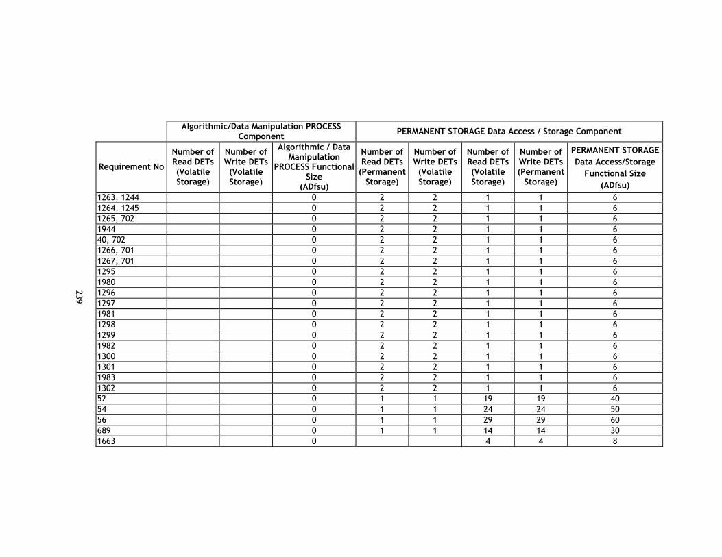
239

Algorithmic/Data Manipulation PROCESS Component PERMANENT STORAGE Data Access / Storage Component

Requirement No

Number of Read DETs (Volatile Storage)

Number of Write DETs (Volatile Storage)

Algorithmic / Data Manipulation

PROCESS Functional Size

(ADfsu)

Number of Read DETs

(Permanent Storage)

Number of Write DETs (Volatile Storage)

Number of Read DETs (Volatile Storage)

Number of Write DETs (Permanent

Storage)

PERMANENT STORAGE Data Access/Storage

Functional Size (ADfsu)

1263, 1244 0 2 2 1 1 6 1264, 1245 0 2 2 1 1 6 1265, 702 0 2 2 1 1 6 1944 0 2 2 1 1 6 40, 702 0 2 2 1 1 6 1266, 701 0 2 2 1 1 6 1267, 701 0 2 2 1 1 6 1295 0 2 2 1 1 6 1980 0 2 2 1 1 6 1296 0 2 2 1 1 6 1297 0 2 2 1 1 6 1981 0 2 2 1 1 6 1298 0 2 2 1 1 6 1299 0 2 2 1 1 6 1982 0 2 2 1 1 6 1300 0 2 2 1 1 6 1301 0 2 2 1 1 6 1983 0 2 2 1 1 6 1302 0 2 2 1 1 6 52 0 1 1 19 19 40 54 0 1 1 24 24 50 56 0 1 1 29 29 60 689 0 1 1 14 14 30 1663 0 4 4 8

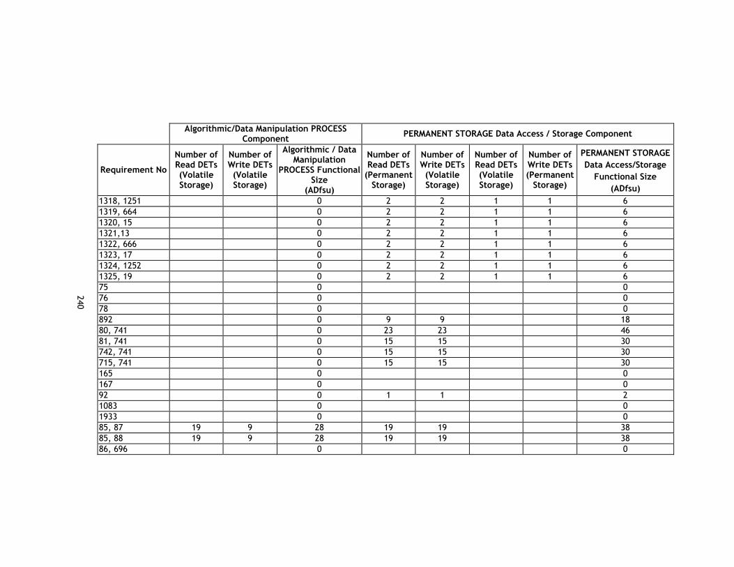
240

Algorithmic/Data Manipulation PROCESS Component PERMANENT STORAGE Data Access / Storage Component

Requirement No

Number of Read DETs (Volatile Storage)

Number of Write DETs (Volatile Storage)

Algorithmic / Data Manipulation

PROCESS Functional Size

(ADfsu)

Number of Read DETs

(Permanent Storage)

Number of Write DETs (Volatile Storage)

Number of Read DETs (Volatile Storage)

Number of Write DETs (Permanent

Storage)

PERMANENT STORAGE Data Access/Storage

Functional Size (ADfsu)

1318, 1251 0 2 2 1 1 6 1319, 664 0 2 2 1 1 6 1320, 15 0 2 2 1 1 6 1321,13 0 2 2 1 1 6 1322, 666 0 2 2 1 1 6 1323, 17 0 2 2 1 1 6 1324, 1252 0 2 2 1 1 6 1325, 19 0 2 2 1 1 6 75 0 0 76 0 0 78 0 0 892 0 9 9 18 80, 741 0 23 23 46 81, 741 0 15 15 30 742, 741 0 15 15 30 715, 741 0 15 15 30 165 0 0 167 0 0 92 0 1 1 2 1083 0 0 1933 0 0 85, 87 19 9 28 19 19 38 85, 88 19 9 28 19 19 38 86, 696 0 0

241

Algorithmic/Data Manipulation PROCESS Component PERMANENT STORAGE Data Access / Storage Component

Requirement No

Number of Read DETs (Volatile Storage)

Number of Write DETs (Volatile Storage)

Algorithmic / Data Manipulation

PROCESS Functional Size

(ADfsu)

Number of Read DETs

(Permanent Storage)

Number of Write DETs (Volatile Storage)

Number of Read DETs (Volatile Storage)

Number of Write DETs (Permanent

Storage)

PERMANENT STORAGE Data Access/Storage

Functional Size (ADfsu)

740, 696 1 2 3 1 1 2 89, 2166, 2163 0 2 2 4 91, 87 19 9 28 19 19 38 91, 88 19 9 28 19 19 38 100 0 6 6 12 101 0 6 6 12 102 0 6 6 12 103 0 6 6 12 104 0 1 1 2 105 0 1 1 2 109, 583, 584 0 7 7 14 1152, 583, 584 0 3 3 6 112 0 5 5 10 113, 578 0 5 5 10 114, 588 0 5 5 10 1059 0 5 5 10 115 0 5 5 10 116 0 1 1 2 2 6 117 0 1 1 2 2 6 118 0 1 1 2 2 6 717 0 1 1 2 2 6 119 0 1 1 1 1 4 120 0 1 1 1 1 4 121 0 1 1 1 1 4

242

Algorithmic/Data Manipulation PROCESS Component PERMANENT STORAGE Data Access / Storage Component

Requirement No

Number of Read DETs (Volatile Storage)

Number of Write DETs (Volatile Storage)

Algorithmic / Data Manipulation

PROCESS Functional Size

(ADfsu)

Number of Read DETs

(Permanent Storage)

Number of Write DETs (Volatile Storage)

Number of Read DETs (Volatile Storage)

Number of Write DETs (Permanent

Storage)

PERMANENT STORAGE Data Access/Storage

Functional Size (ADfsu)

718 0 1 1 1 1 4 719 0 1 1 2 2 6 720 0 1 1 2 2 6 721 0 1 1 2 2 6 722 0 1 1 2 2 6 123, 577, 1051 0 3 3 6 1189 0 3 3 6 124, 577, 1051 0 3 3 6 1190 0 3 3 6 125, 577, 1051 0 3 3 6 1191 0 3 3 6 723, 577, 1051 0 3 3 6 127 0 1 1 2 725 0 0 726 0 0 131 2 1 3 3 3 1 1 8 133 2 1 3 3 3 1 1 8 135 2 1 3 3 3 1 1 8 137 2 1 3 3 3 1 1 8 139 2 1 3 3 3 1 1 8 141 2 1 3 3 3 1 1 8 727 2 1 3 3 3 1 1 8 729 2 1 3 3 3 1 1 8 1138 2 1 3 3 3 6

243

Algorithmic/Data Manipulation PROCESS Component PERMANENT STORAGE Data Access / Storage Component

Requirement No

Number of Read DETs (Volatile Storage)

Number of Write DETs (Volatile Storage)

Algorithmic / Data Manipulation

PROCESS Functional Size

(ADfsu)

Number of Read DETs

(Permanent Storage)

Number of Write DETs (Volatile Storage)

Number of Read DETs (Volatile Storage)

Number of Write DETs (Permanent

Storage)

PERMANENT STORAGE Data Access/Storage

Functional Size (ADfsu)

1139 2 1 3 3 3 6 1140 2 1 3 3 3 6 1141 2 1 3 3 3 6 1142 2 1 3 3 3 6 1143 2 1 3 3 3 6 1144 2 1 3 3 3 6 1145 2 1 3 3 3 6 1148 0 1 1 2 1924 0 1 1 1 1 4 144 0 1 1 1 1 4 1925 0 1 1 1 1 4 146 0 1 1 1 1 4 1926 0 1 1 1 1 4 148 0 1 1 1 1 4 1927 0 1 1 1 1 4 732 0 1 1 1 1 4 151 0 0 152 2 1 3 2 2 4 153 2 1 3 2 2 4 154 2 1 3 2 2 4 155 2 1 3 2 2 4 156 5 1 6 2 2 4 157 5 1 6 2 2 4 736 5 1 6 2 2 4

244

Algorithmic/Data Manipulation PROCESS Component PERMANENT STORAGE Data Access / Storage Component

Requirement No

Number of Read DETs (Volatile Storage)

Number of Write DETs (Volatile Storage)

Algorithmic / Data Manipulation

PROCESS Functional Size

(ADfsu)

Number of Read DETs

(Permanent Storage)

Number of Write DETs (Volatile Storage)

Number of Read DETs (Volatile Storage)

Number of Write DETs (Permanent

Storage)

PERMANENT STORAGE Data Access/Storage

Functional Size (ADfsu)

737 5 1 6 2 2 4 1113 5 1 6 2 2 4 1114 5 1 6 2 2 4 1115 5 1 6 2 2 4 738 5 1 6 2 2 4 739 5 1 6 2 2 4 158 2 1 3 2 2 4 159 2 1 3 2 2 4 160 2 1 3 2 2 4 161 2 1 3 2 2 4 953, 59, 748 0 3 3 1 1 8 953, 58, 747 0 3 3 1 1 8 171, 172 0 3 3 1 1 8 175, 176 0 3 3 1 1 8 179, 180 0 3 3 1 1 8 183, 184 0 3 3 1 1 8 187, 188 0 3 3 1 1 8 191, 192 0 3 3 1 1 8 202, 205, 560, 561

0 3 3 1 1 8

203, 204 0 3 3 1 1 8 206, 209 0 3 3 1 1 8 207, 208 0 3 3 1 1 8 211, 212 0 3 3 1 1 8

245

Algorithmic/Data Manipulation PROCESS Component PERMANENT STORAGE Data Access / Storage Component

Requirement No

Number of Read DETs (Volatile Storage)

Number of Write DETs (Volatile Storage)

Algorithmic / Data Manipulation

PROCESS Functional Size

(ADfsu)

Number of Read DETs

(Permanent Storage)

Number of Write DETs (Volatile Storage)

Number of Read DETs (Volatile Storage)

Number of Write DETs (Permanent

Storage)

PERMANENT STORAGE Data Access/Storage

Functional Size (ADfsu)

210, 213 0 3 3 1 1 8 214, 217 0 3 3 1 1 8 215, 216 0 3 3 1 1 8 750, 751 0 3 3 1 1 8 754, 755 0 3 3 1 1 8 758, 761, 562, 1042

0 3 3 1 1 8

759, 760 0 3 3 1 1 8 762, 765, 557 0 3 3 1 1 8 763, 764 0 3 3 1 1 8 900 0 9 9 18 779, 61 0 3 3 1 1 8 226, 227 0 3 3 1 1 8 786, 787 0 3 3 1 1 8 234, 235 0 3 3 1 1 8 238, 239 0 3 3 1 1 8 242.243 0 3 3 1 1 8 246, 247 0 3 3 1 1 8 250, 251 0 3 3 1 1 8 253, 256, 555, 556

0 3 3 1 1 8

254, 255 0 3 3 1 1 8 257, 260 0 3 3 1 1 8 258, 259 0 3 3 1 1 8

246

Algorithmic/Data Manipulation PROCESS Component PERMANENT STORAGE Data Access / Storage Component

Requirement No

Number of Read DETs (Volatile Storage)

Number of Write DETs (Volatile Storage)

Algorithmic / Data Manipulation

PROCESS Functional Size

(ADfsu)

Number of Read DETs

(Permanent Storage)

Number of Write DETs (Volatile Storage)

Number of Read DETs (Volatile Storage)

Number of Write DETs (Permanent

Storage)

PERMANENT STORAGE Data Access/Storage

Functional Size (ADfsu)

261, 264 0 3 3 1 1 8 262, 263 0 3 3 1 1 8 265, 268 0 3 3 1 1 8 266, 267 0 3 3 1 1 8 790, 791 0 3 3 1 1 8 793, 796, 562, 1042

0 3 3 1 1 8

794, 795 0 3 3 1 1 8 806, 807 0 3 3 1 1 8 810, 811 0 3 3 1 1 8 814, 815 0 3 3 1 1 8 819, 745 0 3 3 1 1 8 276, 277 0 3 3 1 1 8 280, 281 0 3 3 1 1 8 284, 285 0 3 3 1 1 8 288, 289 0 3 3 1 1 8 292, 293 0 3 3 1 1 8 300, 301 0 3 3 1 1 8 304, 305 0 3 3 1 1 8 303, 306 0 3 3 1 1 8 308, 309 0 3 3 1 1 8 307, 310 0 3 3 1 1 8 311, 314 0 3 3 1 1 8 312, 313 0 3 3 1 1 8

247

Algorithmic/Data Manipulation PROCESS Component PERMANENT STORAGE Data Access / Storage Component

Requirement No

Number of Read DETs (Volatile Storage)

Number of Write DETs (Volatile Storage)

Algorithmic / Data Manipulation

PROCESS Functional Size

(ADfsu)

Number of Read DETs

(Permanent Storage)

Number of Write DETs (Volatile Storage)

Number of Read DETs (Volatile Storage)

Number of Write DETs (Permanent

Storage)

PERMANENT STORAGE Data Access/Storage

Functional Size (ADfsu)

316, 317 0 3 3 1 1 8 825, 826 0 3 3 1 1 8 829, 830 0 3 3 1 1 8 833, 834 0 3 3 1 1 8 837, 838 0 3 3 1 1 8 841, 842 0 3 3 1 1 8 844, 847 0 3 3 1 1 8 845, 846 0 3 3 1 1 8 849, 850 0 3 3 1 1 8 853, 854 0 3 3 1 1 8 856, 859 0 3 3 1 1 8 857, 858 0 3 3 1 1 8 860, 863 0 3 3 1 1 8 861, 862 0 3 3 1 1 8 865, 866 0 3 3 1 1 8 869, 870 0 3 3 1 1 8 884 0 9 9 18 878, 63 0 3 3 1 1 8 879, 882 0 3 3 1 1 8 880, 881 0 3 3 1 1 8 1120, 1122 0 3 3 1 1 8 1121, 1123 0 3 3 1 1 8 1125, 1127 0 3 3 1 1 8 905, 907 0 3 3 1 1 8

248

Algorithmic/Data Manipulation PROCESS Component PERMANENT STORAGE Data Access / Storage Component

Requirement No

Number of Read DETs (Volatile Storage)

Number of Write DETs (Volatile Storage)

Algorithmic / Data Manipulation

PROCESS Functional Size

(ADfsu)

Number of Read DETs

(Permanent Storage)

Number of Write DETs (Volatile Storage)

Number of Read DETs (Volatile Storage)

Number of Write DETs (Permanent

Storage)

PERMANENT STORAGE Data Access/Storage

Functional Size (ADfsu)

911, 913 0 3 3 1 1 8 912, 914 0 3 3 1 1 8 1117, 1119 0 3 3 1 1 8 915, 917 0 3 3 1 1 8 916, 918 0 3 3 1 1 8 928, 930 0 3 3 1 1 8 929, 931 0 3 3 1 1 8 934, 936 0 3 3 1 1 8 1940 0 0 90 0 0 321 4 1 5 2 2 4 941 0 0 942 0 0 943 0 0 333 2 2 4 1 1 2 334 2 2 4 1 1 2 322 5 1 6 5 5 10 323 5 1 6 5 5 10 324 5 1 6 5 5 10 325 5 1 6 5 5 10 326 5 1 6 5 5 10 327 5 1 6 5 5 10 328 5 1 6 5 5 10 329 5 1 6 5 5 10

249

Algorithmic/Data Manipulation PROCESS Component PERMANENT STORAGE Data Access / Storage Component

Requirement No

Number of Read DETs (Volatile Storage)

Number of Write DETs (Volatile Storage)

Algorithmic / Data Manipulation

PROCESS Functional Size

(ADfsu)

Number of Read DETs

(Permanent Storage)

Number of Write DETs (Volatile Storage)

Number of Read DETs (Volatile Storage)

Number of Write DETs (Permanent

Storage)

PERMANENT STORAGE Data Access/Storage

Functional Size (ADfsu)

330 5 1 6 5 5 10 335 0 0 372 0 2 2 4 373 0 2 2 4 341 0 2 2 4 342 0 2 2 4 343 0 2 2 4 344 0 2 2 4 1061 0 2 2 4 345 0 2 2 4 346 0 2 2 4 1068 0 2 2 4 2113,..,2122, 2040, 2162, 378, 178, 181, 541, 549

6 11 17 43 43 9 1 96

2113,..,2122, 376, 2162, 378, 178, 181, 541, 549

6 11 17 44 44 9 1 98

2113,..,2122, 944, 2162, 378, 178, 181, 541, 549

7 12 19 49 49 9 1 108

2113,..,2122, 6 11 17 48 48 9 1 106

250

Algorithmic/Data Manipulation PROCESS Component PERMANENT STORAGE Data Access / Storage Component

Requirement No

Number of Read DETs (Volatile Storage)

Number of Write DETs (Volatile Storage)

Algorithmic / Data Manipulation

PROCESS Functional Size

(ADfsu)

Number of Read DETs

(Permanent Storage)

Number of Write DETs (Volatile Storage)

Number of Read DETs (Volatile Storage)

Number of Write DETs (Permanent

Storage)

PERMANENT STORAGE Data Access/Storage

Functional Size (ADfsu)

945, 2162, 378, 178, 181, 541, 549 383, 385,2123,.., 2126, 170, 173, 177, 174

6 11 17 21 21 10 2 54

946, 949, 2123,.., 2126, 170, 173, 177, 174

6 11 17 22 22 10 2 56

2131, 387, 749, 752, 545

4 9 13 13 13 9 1 36

2127, 406, 249, 252, 543

4 9 13 13 13 9 1 36

2128, 2130, 408, 249, 252, 544

4 9 13 13 13 9 1 36

2150, 411, 233, 236, 547

6 11 17 20 20 9 1 50

2150, 961, 233, 236, 547

6 11 17 21 21 9 1 52

2150, 413, 233, 236, 547

5 10 15 20 20 9 1 50

2139, 2140, 418, 805, 808, 548

4 9 13 15 15 9 1 40

2141,...2149, 4 9 13 39 39 9 1 88

251

Algorithmic/Data Manipulation PROCESS Component PERMANENT STORAGE Data Access / Storage Component

Requirement No

Number of Read DETs (Volatile Storage)

Number of Write DETs (Volatile Storage)

Algorithmic / Data Manipulation

PROCESS Functional Size

(ADfsu)

Number of Read DETs

(Permanent Storage)

Number of Write DETs (Volatile Storage)

Number of Read DETs (Volatile Storage)

Number of Write DETs (Permanent

Storage)

PERMANENT STORAGE Data Access/Storage

Functional Size (ADfsu)

420, 237, 240, 546 2133,.., 2138, 523, 550, 753, 756

4 9 13 25 25 9 1 60

2141,...2149, 392, 546, 182, 185

4 9 13 39 39 9 1 88

2113,..,2122, 2041, 541, 397, 2162, 549

5 11 16 41 41 8 90

2113,..,2122, 395, 541, 397, 2162, 549

6 11 17 42 42 8 92

2113,..,2122, 954, 541, 397, 2162, 549

7 12 19 47 47 8 102

2113,..,2122, 955, 541, 397, 2162, 549

6 11 17 46 46 8 100

2123,.., 2126, 401, 402, 542, 228, 225

6 11 17 21 21 10 2 54

2123,.., 2126, 958, 959, 542,

6 11 17 22 22 10 2 56

252

Algorithmic/Data Manipulation PROCESS Component PERMANENT STORAGE Data Access / Storage Component

Requirement No

Number of Read DETs (Volatile Storage)

Number of Write DETs (Volatile Storage)

Algorithmic / Data Manipulation

PROCESS Functional Size

(ADfsu)

Number of Read DETs

(Permanent Storage)

Number of Write DETs (Volatile Storage)

Number of Read DETs (Volatile Storage)

Number of Write DETs (Permanent

Storage)

PERMANENT STORAGE Data Access/Storage

Functional Size (ADfsu)

228, 225 2131, 404, 785, 788, 545

4 9 13 13 13 9 1 36

2133,.., 2138, 964, 789, 792, 550

4 9 13 25 25 9 1 60

2132, 966, 809, 812, 1774

4 9 13 13 13 9 1 36

965, 778, 60 0 5 5 1 1 12 424 0 1 1 2 2113,..,2122, 2042, 286, 283, 541, 428, 2162, 549

6 11 17 43 43 9 1 96

2113,..,2122,426, 286, 283, 541, 428, 2162, 549

6 11 17 44 44 9 1 98

2113,..,2122, 967, 286, 283, 541, 428, 2162, 549

7 12 19 49 49 9 1 108

2113,..,2122, 968, 286, 283, 541, 428, 2162, 549

6 11 17 48 48 9 1 106

253

Algorithmic/Data Manipulation PROCESS Component PERMANENT STORAGE Data Access / Storage Component

Requirement No

Number of Read DETs (Volatile Storage)

Number of Write DETs (Volatile Storage)

Algorithmic / Data Manipulation

PROCESS Functional Size

(ADfsu)

Number of Read DETs

(Permanent Storage)

Number of Write DETs (Volatile Storage)

Number of Read DETs (Volatile Storage)

Number of Write DETs (Permanent

Storage)

PERMANENT STORAGE Data Access/Storage

Functional Size (ADfsu)

2123,.., 2126, 432, 275, 278, 542, 433, 282, 279, 549

6 11 17 21 21 10 2 54

2123,.., 2126, 971, 275, 278, 542,, 972, 282, 279

6 11 17 22 22 10 2 56

2131, 435, 315, 318, 545

4 9 13 13 13 9 1 36

2127, 437, 827, 824, 543

4 9 13 13 13 9 1 36

2128, 2130, 441, 827, 824, 544

4 9 13 13 13 9 1 36

2150, 443, 290, 287, 547

6 11 17 20 20 9 1 50

2150, 974, 290, 287, 547

6 11 17 21 21 9 1 52

2150, 976, 290, 287, 547

5 10 15 20 20 9 1 50

2139, 2140, 445, 848, 851, 548

4 9 13 15 15 9 1 40

2141,...2149, 980, 828, 831, 546

4 9 13 39 39 9 1 88

254

Algorithmic/Data Manipulation PROCESS Component PERMANENT STORAGE Data Access / Storage Component

Requirement No

Number of Read DETs (Volatile Storage)

Number of Write DETs (Volatile Storage)

Algorithmic / Data Manipulation

PROCESS Functional Size

(ADfsu)

Number of Read DETs

(Permanent Storage)

Number of Write DETs (Volatile Storage)

Number of Read DETs (Volatile Storage)

Number of Write DETs (Permanent

Storage)

PERMANENT STORAGE Data Access/Storage

Functional Size (ADfsu)

2132, 983, 852, 855, 1774

4 9 13 13 13 9 1 36

984, 818, 62 0 5 5 1 1 12 2133,.., 2138, 987, 832, 835, 550

4 9 13 25 25 9 1 60

2113,..,2122, 2043, 1122,1120, 541, 1131, 549, 2162

5 11 16 43 43 9 1 96

2113,..,2122, 1128, 1122,1120, 541, 1131, 549, 2162

6 11 17 44 44 9 1 98

2113,..,2122, 1129, 1122,1120, 541, 1131, 549, 2162

7 12 19 49 49 9 1 108

2113,..,2122, 1130, 1122,1120, 541, 1131, 549, 2162

6 11 17 48 48 9 1 106

2133,.., 2138, 1156, 904, 906, 550

4 9 13 25 25 9 1 60

255

Algorithmic/Data Manipulation PROCESS Component PERMANENT STORAGE Data Access / Storage Component

Requirement No

Number of Read DETs (Volatile Storage)

Number of Write DETs (Volatile Storage)

Algorithmic / Data Manipulation

PROCESS Functional Size

(ADfsu)

Number of Read DETs

(Permanent Storage)

Number of Write DETs (Volatile Storage)

Number of Read DETs (Volatile Storage)

Number of Write DETs (Permanent

Storage)

PERMANENT STORAGE Data Access/Storage

Functional Size (ADfsu)

1157, 877, 746 0 5 5 1 1 12 521 15 15 3 4 7 1011 9 9 3 3 6 1013 15 15 3 4 7 1012 9 9 3 3 6 1135 15 15 3 4 7 1136 9 9 3 3 6 524.555.556 4 9 13 18 19 37 525 5 10 15 16 17 33 527 6 11 17 16 17 33 529 6 11 17 14 15 29 990 5 10 15 11 12 23 531 4 9 13 20 21 41 533 4 9 13 20 21 41 535, 253, 256, 555, 556

4 9 13 20 21 41

536 4 9 13 20 21 41 992 5 10 15 16 17 33 994, 813, 816, 557

6 11 17 16 17 33

996, 813, 816, 557

6 11 17 14 15 29

998, 813, 816, 557

5 10 15 11 12 23

1000, 299, 302, 4 9 13 20 21 1 1 43

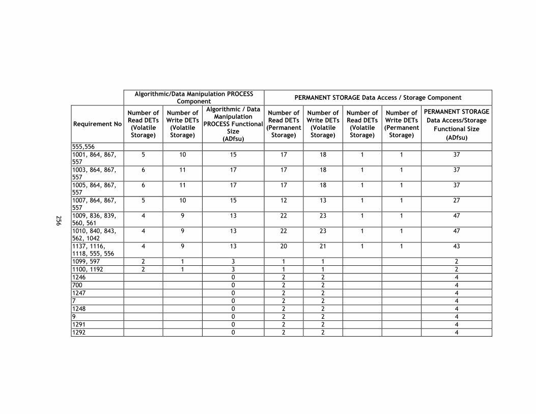
256

Algorithmic/Data Manipulation PROCESS Component PERMANENT STORAGE Data Access / Storage Component

Requirement No

Number of Read DETs (Volatile Storage)

Number of Write DETs (Volatile Storage)

Algorithmic / Data Manipulation

PROCESS Functional Size

(ADfsu)

Number of Read DETs

(Permanent Storage)

Number of Write DETs (Volatile Storage)

Number of Read DETs (Volatile Storage)

Number of Write DETs (Permanent

Storage)

PERMANENT STORAGE Data Access/Storage

Functional Size (ADfsu)

555,556 1001, 864, 867, 557

5 10 15 17 18 1 1 37

1003, 864, 867, 557

6 11 17 17 18 1 1 37

1005, 864, 867, 557

6 11 17 17 18 1 1 37

1007, 864, 867, 557

5 10 15 12 13 1 1 27

1009, 836, 839, 560, 561

4 9 13 22 23 1 1 47

1010, 840, 843, 562, 1042

4 9 13 22 23 1 1 47

1137, 1116, 1118, 555, 556

4 9 13 20 21 1 1 43

1099, 597 2 1 3 1 1 2 1100, 1192 2 1 3 1 1 2 1246 0 2 2 4 700 0 2 2 4 1247 0 2 2 4 7 0 2 2 4 1248 0 2 2 4 9 0 2 2 4 1291 0 2 2 4 1292 0 2 2 4

257

Algorithmic/Data Manipulation PROCESS Component PERMANENT STORAGE Data Access / Storage Component

Requirement No

Number of Read DETs (Volatile Storage)

Number of Write DETs (Volatile Storage)

Algorithmic / Data Manipulation

PROCESS Functional Size

(ADfsu)

Number of Read DETs

(Permanent Storage)

Number of Write DETs (Volatile Storage)

Number of Read DETs (Volatile Storage)

Number of Write DETs (Permanent

Storage)

PERMANENT STORAGE Data Access/Storage

Functional Size (ADfsu)

1293 0 2 2 4 1282 0 0 1283 0 0 1284 0 2 2 4 1285 0 2 2 4 1286 0 2 2 4 1287 0 2 2 4 46 0 2 2 4 1288 0 2 2 4 1289 0 2 2 4 1290 0 2 2 4 75 0 0 76 0 0 78 0 0 CUSTOM -291, 294, 2152, 2154, 970, 2153, 2093, 430, 969, 1002, 1004, 1006, 1008, 2159, 434, 973, 2161, 436, 2157, 438, 2160, 442, 2151, 975, 444, 978, 2158, 446, 2155, 981

17 23 40 112 112 9 1 234

258

Algorithmic/Data Manipulation PROCESS Component PERMANENT STORAGE Data Access / Storage Component

Requirement No

Number of Read DETs (Volatile Storage)

Number of Write DETs (Volatile Storage)

Algorithmic / Data Manipulation

PROCESS Functional Size

(ADfsu)

Number of Read DETs

(Permanent Storage)

Number of Write DETs (Volatile Storage)

Number of Read DETs (Volatile Storage)

Number of Write DETs (Permanent

Storage)

PERMANENT STORAGE Data Access/Storage

Functional Size (ADfsu)

IFR-241, 244, 993, 995, 997, 999, 2159, 403, 960, 2161, 405, 2155, 421, 2152, 2153,2154, 399, 2092, 956, 957, 2160, 409, 2157, 407, 2158, 1155, 2151, 412, 414, 962

17 23 40 112 112 9 1 234

VFR-186, 189, 2159, 386, 950, 2161, 388, 991, 526, 530, 528, 2155, 393, 2152, 2154, 380, 947, 948, 2153, 2095

13 15 28 56 56 9 1 122

WSI - 1124, 1126, 2153, 2094, 2152, 2154, 1132, 1133, 1134

7 7 14 41 41 9 1 92

564 0 0 567 0 0 193, 451, 565 2 1 3 5 5 1 1 12

259

Algorithmic/Data Manipulation PROCESS Component PERMANENT STORAGE Data Access / Storage Component

Requirement No

Number of Read DETs (Volatile Storage)

Number of Write DETs (Volatile Storage)

Algorithmic / Data Manipulation

PROCESS Functional Size

(ADfsu)

Number of Read DETs

(Permanent Storage)

Number of Write DETs (Volatile Storage)

Number of Read DETs (Volatile Storage)

Number of Write DETs (Permanent

Storage)

PERMANENT STORAGE Data Access/Storage

Functional Size (ADfsu)

777, 451, 565 2 1 3 5 5 1 1 12 248, 1208, 565 2 1 3 5 5 1 1 12 780, 1208, 565 2 1 3 5 5 1 1 12 871, 1209, 565 2 1 3 5 5 1 1 12 872, 1209, 565 2 1 3 5 5 1 1 12 935, 1210, 565 2 1 3 5 5 1 1 12 1060, 1210, 565 2 1 3 5 5 1 1 12 1212 0 0 1211 0 0 1213 0 0 1224, 1215, 1216 2 1 3 1 1 2 1224, 1214, 1217, 1218

2 1 3 1 1 2

1225, 1215, 1216 2 1 3 1 1 2 1225, 1214, 1217, 1218

2 1 3 1 1 2

454, 1215, 1216 4 3 7 4 4 8 454, 1214, 1217, 1218

4 3 7 4 4 8

456, 1219, 1220, 1221, 1215, 1216

5 3 8 5 5 10

456, 1219, 1220, 1221, 1214, 1217, 1218

5 3 8 5 5 10

1222, 1223, 2 1 3 1 1 2

260

Algorithmic/Data Manipulation PROCESS Component PERMANENT STORAGE Data Access / Storage Component

Requirement No

Number of Read DETs (Volatile Storage)

Number of Write DETs (Volatile Storage)

Algorithmic / Data Manipulation

PROCESS Functional Size

(ADfsu)

Number of Read DETs

(Permanent Storage)

Number of Write DETs (Volatile Storage)

Number of Read DETs (Volatile Storage)

Number of Write DETs (Permanent

Storage)

PERMANENT STORAGE Data Access/Storage

Functional Size (ADfsu)

1215, 1216 1222, 1223, 1214, 1217, 1218

2 1 3 1 1 2

459, 1014, 1215, 1216

2 1 3 2 2 4

459, 1014, 1214, 1217, 1218

2 1 3 2 2 4

461 2 2 4 0 467, 468, 1215, 1216

2 1 3 6 6 12

467, 468, 1214, 1217, 1218

2 1 3 5 5 10

470 0 1 1 2 519, 1215, 1216 4 3 7 2 2 4

Total 687 941 1,628 2,983 3,007 734 334 7,058

261

INTERFACE Component Control PROCESS Component

Requirement No Number of Read DETs

(I/O Device)

Number of Write DETs (Volatile Storage)

Number of Read DETs (Volatile Storage)

Number of Write DETs (I/O Device)

INTERFACE Functional

Size (ADfsu)

Number of Read DETs (Volatile Storage)

Number of Write DETs (Volatile Storage)

Control PROCESS Functional Size

(ADfsu)

1640, 2170, 1632 3 3 5 5 16 4 4

2064, 2170, 1632 4 4 5 5 18 4 4

1641, 2169, 1632 3 3 5 5 16 4 4

2065, 2169, 1632 4 4 5 5 18 4 4

1642, 2167, 1632 3 3 5 5 16 4 4

2066, 2167, 1632 4 4 5 5 18 4 4

1643, 2168, 1632 3 3 5 5 16 4 4

2067, 2168, 1632 4 4 5 5 18 4 4

2068, 2170, 1632 3 3 5 5 16 4 4

2069, 2170, 1632 4 4 5 5 18 4 4

2070, 2169, 1632 3 3 5 5 16 4 4

2071, 2169, 1632 4 4 5 5 18 4 4

2072, 2167, 1632 3 3 5 5 16 4 4

2073, 2167, 1632 4 4 5 5 18 4 4

2074, 2168, 1632 3 3 5 5 16 4 4

2075, 2168, 1632 4 4 5 5 18 4 4

2076, 2170, 1632 3 3 5 5 16 4 4

2077, 2170, 1632 4 4 5 5 18 4 4

2078, 2169, 1632 3 3 5 5 16 4 4

Case Study 3.1 - Subsystem B – A

RCHI-D

IM FSM

Measurem

ent Catalogue

262

INTERFACE Component Control PROCESS Component

Requirement No Number of Read DETs

(I/O Device)

Number of Write DETs (Volatile Storage)

Number of Read DETs (Volatile Storage)

Number of Write DETs (I/O Device)

INTERFACE Functional

Size (ADfsu)

Number of Read DETs (Volatile Storage)

Number of Write DETs (Volatile Storage)

Control PROCESS Functional Size

(ADfsu)

2079, 2169, 1632 4 4 5 5 18 4 4

2080, 2167, 1632 3 3 5 5 16 4 4

2081, 2167, 1632 4 4 5 5 18 4 4

2082, 2168, 1632 3 3 5 5 16 4 4

2083, 2168, 1632 4 4 5 5 18 4 4

2083, 2169,1632

2084, 2170, 1632 3 3 5 5 16 4 4

2085, 2170, 1632 4 4 5 5 18 4 4

2086, 2169, 1632 3 3 5 5 16 4 4

2087, 2169, 1632 4 4 5 5 18 4 4

2088, 2167, 1632 3 3 5 5 16 4 4

2089, 2167, 1632 4 4 5 5 18 4 4

2090, 2168, 1632 3 3 5 5 16 4 4

2091, 2168, 1632 4 4 5 5 18 4 4

Total 112,00 112,00 160,00 160,00 544,00 128,00 0,00 128,00

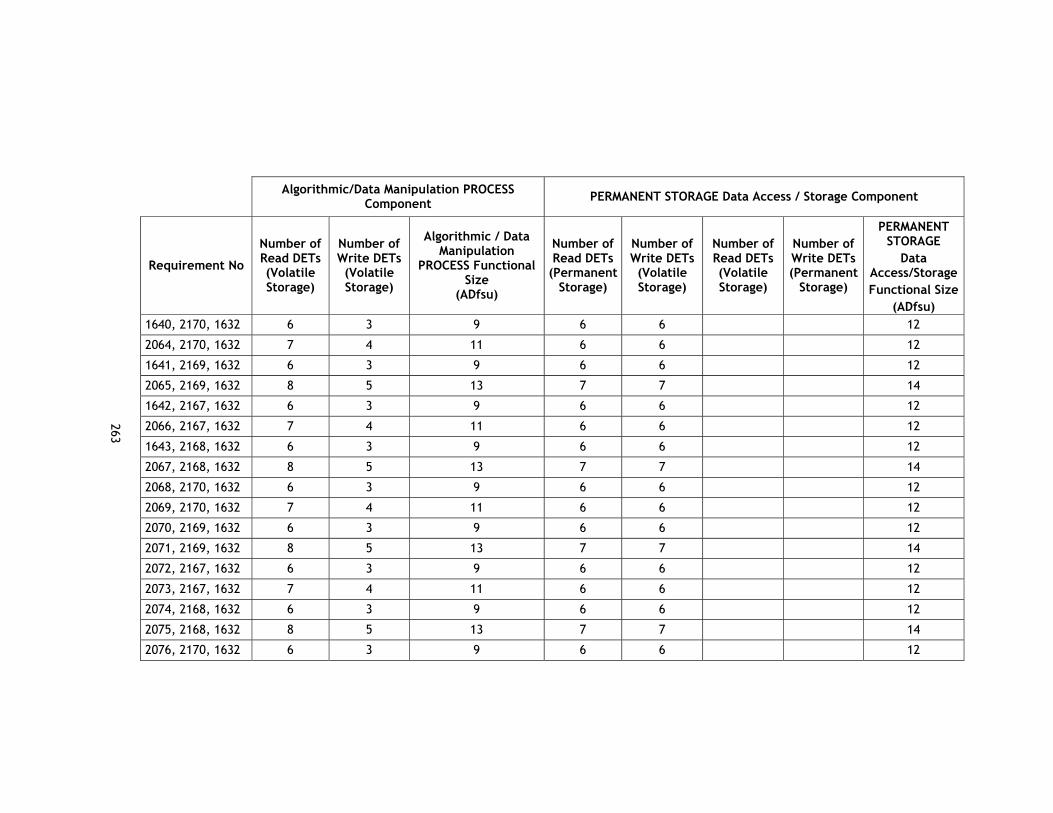
263

Algorithmic/Data Manipulation PROCESS Component PERMANENT STORAGE Data Access / Storage Component

Requirement No

Number of Read DETs (Volatile Storage)

Number of Write DETs (Volatile Storage)

Algorithmic / Data Manipulation

PROCESS Functional Size

(ADfsu)

Number of Read DETs

(Permanent Storage)

Number of Write DETs (Volatile Storage)

Number of Read DETs (Volatile Storage)

Number of Write DETs (Permanent

Storage)

PERMANENT STORAGE

Data Access/Storage Functional Size

(ADfsu) 1640, 2170, 1632 6 3 9 6 6 12

2064, 2170, 1632 7 4 11 6 6 12

1641, 2169, 1632 6 3 9 6 6 12

2065, 2169, 1632 8 5 13 7 7 14

1642, 2167, 1632 6 3 9 6 6 12

2066, 2167, 1632 7 4 11 6 6 12

1643, 2168, 1632 6 3 9 6 6 12

2067, 2168, 1632 8 5 13 7 7 14

2068, 2170, 1632 6 3 9 6 6 12

2069, 2170, 1632 7 4 11 6 6 12

2070, 2169, 1632 6 3 9 6 6 12

2071, 2169, 1632 8 5 13 7 7 14

2072, 2167, 1632 6 3 9 6 6 12

2073, 2167, 1632 7 4 11 6 6 12

2074, 2168, 1632 6 3 9 6 6 12

2075, 2168, 1632 8 5 13 7 7 14

2076, 2170, 1632 6 3 9 6 6 12

264

Algorithmic/Data Manipulation PROCESS Component PERMANENT STORAGE Data Access / Storage Component

Requirement No

Number of Read DETs (Volatile Storage)

Number of Write DETs (Volatile Storage)

Algorithmic / Data Manipulation

PROCESS Functional Size

(ADfsu)

Number of Read DETs

(Permanent Storage)

Number of Write DETs (Volatile Storage)

Number of Read DETs (Volatile Storage)

Number of Write DETs (Permanent

Storage)

PERMANENT STORAGE

Data Access/Storage Functional Size

(ADfsu) 2077, 2170, 1632 7 4 11 6 6 12

2078, 2169, 1632 6 3 9 6 6 12

2079, 2169, 1632 8 5 13 7 7 14

2080, 2167, 1632 6 3 9 6 6 12

2081, 2167, 1632 7 4 11 6 6 12

2082, 2168, 1632 6 3 9 6 6 12

2083, 2168, 1632 8 5 13 7 7 14

2083, 2169,1632

2084, 2170, 1632 6 3 9 6 6 12

2085, 2170, 1632 7 4 11 6 6 12

2086, 2169, 1632 6 3 9 6 6 12

2087, 2169, 1632 8 5 13 7 7 14

2088, 2167, 1632 6 3 9 6 6 12

2089, 2167, 1632 7 4 11 6 6 12

2090, 2168, 1632 6 3 9 6 6 12

2091, 2168, 1632 8 5 13 7 7 14

Total 216,00 120,00 336,00 200,00 200,00 0,00 0,00 400,00

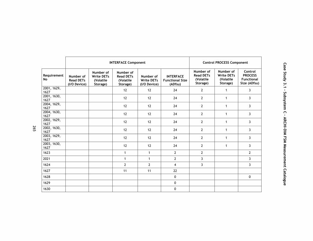
265

INTERFACE Component Control PROCESS Component

Requirement No

Number of Read DETs

(I/O Device)

Number of Write DETs (Volatile Storage)

Number of Read DETs (Volatile Storage)

Number of Write DETs (I/O Device)

INTERFACE Functional Size

(ADfsu)

Number of Read DETs (Volatile Storage)

Number of Write DETs (Volatile Storage)

Control PROCESS

Functional Size (ADfsu)

2001, 1629, 1627 12 12 24 2 1 3

2001, 1630, 1627 12 12 24 2 1 3

2004, 1629, 1627 12 12 24 2 1 3

2004, 1630, 1627 12 12 24 2 1 3

2002, 1629, 1627 12 12 24 2 1 3

2002, 1630, 1627 12 12 24 2 1 3

2003, 1629, 1627 12 12 24 2 1 3

2003, 1630, 1627 12 12 24 2 1 3

1623 1 1 2 2 2

2021 1 1 2 3 3

1624 2 2 4 3 3

1627 11 11 22

1628 0 0

1629 0

1630 0

Case Study 3.1 - Subsystem C – A

RCHI-D

IM FSM

Measurem

ent Catalogue

266

INTERFACE Component Control PROCESS Component

Requirement No

Number of Read DETs

(I/O Device)

Number of Write DETs (Volatile Storage)

Number of Read DETs (Volatile Storage)

Number of Write DETs (I/O Device)

INTERFACE Functional Size

(ADfsu)

Number of Read DETs (Volatile Storage)

Number of Write DETs (Volatile Storage)

Control PROCESS

Functional Size (ADfsu)

1609 1 1 2 2 2

2005 1 1 2 2 2

1610 1 1 2 2 2

2006 1 1 2 2 2

2007 1 1 2 2 2

1611 1 1 2 2 2

2008 1 1 2 2 2

2009 1 1 2 2 2

1338 1 1 2 2 2

2011 1 1 2 2 2

1339 1 1 2 2 2

2012 1 1 2 2 2

1337 1 1 2 3 3

2010 1 1 2 3 3

2010.1 0 0

2013 1 1 2 3 3

2014 1 1 2 3 3

2015 1 1 2 3 3

2016 1 1 2 3 3

267

INTERFACE Component Control PROCESS Component

Requirement No

Number of Read DETs

(I/O Device)

Number of Write DETs (Volatile Storage)

Number of Read DETs (Volatile Storage)

Number of Write DETs (I/O Device)

INTERFACE Functional Size

(ADfsu)

Number of Read DETs (Volatile Storage)

Number of Write DETs (Volatile Storage)

Control PROCESS

Functional Size (ADfsu)

2017 1 1 2 3 3

2018 1 1 2 3 3

2019 1 1 2 3 3

2020 1 1 2 3 3

1587 3 3 6 0

1615 3 3 5 5 16 2 2

1989 3 3 5 5 16 2 2

1991 2 2 4 6 6

1993 2 2 4 6 6

1992 2 2 4 6 6

1994 2 2 4 6 6

Total 9 9 151 151 320.0 106 8 114.0

268

Algorithmic/Data Manipulation PROCESS Component PERMANENT STORAGE Data Access / Storage Component

Requirement No

Number of Read DETs (Volatile Storage)

Number of Write DETs (Volatile Storage)

Algorithmic / Data Manipulation

PROCESS Functional Size

(ADfsu)

Number of Read DETs

(Permanent Storage)

Number of Write DETs (Volatile Storage)

Number of Read DETs (Volatile Storage)

Number of Write DETs (Permanent

Storage)

PERMANENT STORAGE

Data Access/Storage Functional Size

(ADfsu) 2001, 1629, 1627 3 3 6 7 7 14

2001, 1630, 1627 3 3 6 7 7 14

2004, 1629, 1627 6 5 11 8 8 16

2004, 1630, 1627 6 5 11 8 8 16

2002, 1629, 1627 3 3 6 7 7 14

2002, 1630, 1627 3 3 6 7 7 14

2003, 1629, 1627 6 5 11 8 8 16

2003, 1630, 1627 6 5 11 8 8 16

1623 0 0

2021 0 0

1624 0 0

1627 0 3 3 6

1628 0 0

1629 3 3 6 3 3 6

1630 3 3 6 3 3 6

1609 0 2 2 4

2005 3 2 5 3 3 6

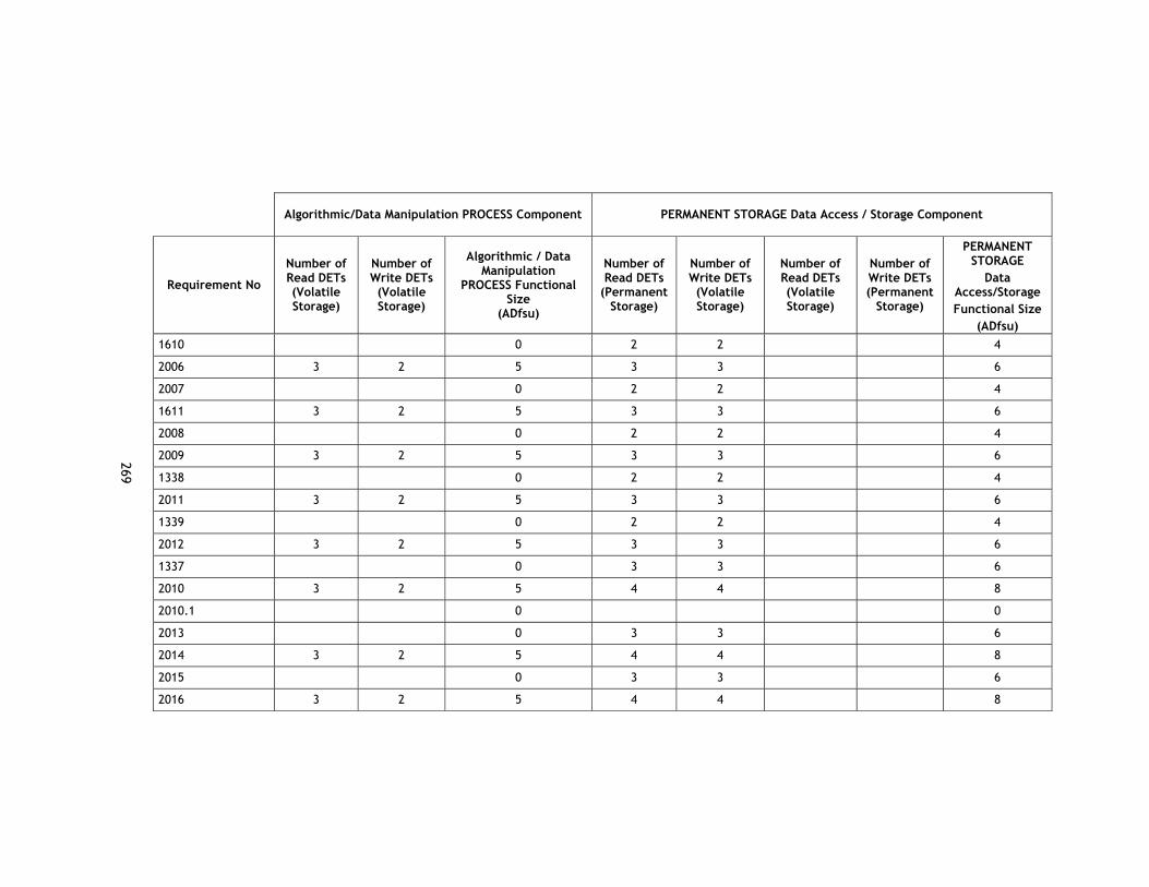
269

Algorithmic/Data Manipulation PROCESS Component PERMANENT STORAGE Data Access / Storage Component

Requirement No

Number of Read DETs (Volatile Storage)

Number of Write DETs (Volatile Storage)

Algorithmic / Data Manipulation

PROCESS Functional Size

(ADfsu)

Number of Read DETs

(Permanent Storage)

Number of Write DETs (Volatile Storage)

Number of Read DETs (Volatile Storage)

Number of Write DETs (Permanent

Storage)

PERMANENT STORAGE

Data Access/Storage Functional Size

(ADfsu) 1610 0 2 2 4

2006 3 2 5 3 3 6

2007 0 2 2 4

1611 3 2 5 3 3 6

2008 0 2 2 4

2009 3 2 5 3 3 6

1338 0 2 2 4

2011 3 2 5 3 3 6

1339 0 2 2 4

2012 3 2 5 3 3 6

1337 0 3 3 6

2010 3 2 5 4 4 8

2010.1 0 0

2013 0 3 3 6

2014 3 2 5 4 4 8

2015 0 3 3 6

2016 3 2 5 4 4 8

270

Algorithmic/Data Manipulation PROCESS Component PERMANENT STORAGE Data Access / Storage Component

Requirement No

Number of Read DETs (Volatile Storage)

Number of Write DETs (Volatile Storage)

Algorithmic / Data Manipulation

PROCESS Functional Size

(ADfsu)

Number of Read DETs

(Permanent Storage)

Number of Write DETs (Volatile Storage)

Number of Read DETs (Volatile Storage)

Number of Write DETs (Permanent

Storage)

PERMANENT STORAGE

Data Access/Storage Functional Size

(ADfsu) 2017 0 3 3 6

2018 3 2 5 4 4 8

2019 0 3 3 6

2020 3 2 5 4 4 8

1587 0 0

1615 5 4 9 3 3 6

1989 5 4 9 3 3 6

1991 2 2 4 2 2 8 12

1993 2 2 4 2 2 8 12

1992 5 4 9 3 3 8 14

1994 5 4 9 3 3 8 14

Total 99 80 179 150 150 32 0 332

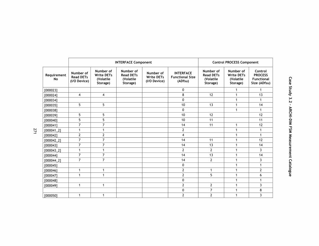
271

Case Study 3.2 – ARCHI-DIM FSM Measurement Catalogue

INTERFACE Component Control PROCESS Component

Requirement No

Number of Read DETs

(I/O Device)

Number of Write DETs (Volatile Storage)

Number of Read DETs (Volatile Storage)

Number of Write DETs (I/O Device)

INTERFACE Functional Size

(ADfsu)

Number of Read DETs (Volatile Storage)

Number of Write DETs (Volatile Storage)

Control PROCESS

Functional Size (ADfsu)

[000023] 0 1 1

[000024] 4 4 8 12 1 13

[000034] 0 1 1

[000035] 5 5 10 13 1 14

[000038] 0 1 1

[000039] 5 5 10 12 12

[000040] 5 5 10 11 11

[000041] 7 7 14 11 1 12

[000041_2] 1 1 2 1 1

[000042] 2 2 4 1 1

[000042_2] 7 7 14 11 1 12

[000043] 7 7 14 13 1 14

[000043_2] 1 1 2 2 1 3

[000044] 7 7 14 13 1 14

[000044_2] 7 7 14 2 1 3

[000045] 0 1 1

[000046] 1 1 2 1 1 2

[000047] 1 1 2 5 1 6

[000048] 0 1 1

[000049] 1 1 2 2 1 3

0 7 1 8

[000050] 1 1 2 2 1 3

Case Study 3.2 – ARCH

I-DIM

FSM M

easurement Catalogue

272

INTERFACE Component Control PROCESS Component

Requirement No

Number of Read DETs

(I/O Device)

Number of Write DETs (Volatile Storage)

Number of Read DETs (Volatile Storage)

Number of Write DETs (I/O Device)

INTERFACE Functional Size

(ADfsu)

Number of Read DETs (Volatile Storage)

Number of Write DETs (Volatile Storage)

Control PROCESS

Functional Size (ADfsu)

0 4 1 5

2 2 4 5 1 6

2 2 4 3 1 4

[000051] T1 5 5 10 17 1 18

T2 5 5 10 15 1 16

T3 5 5 10 15 1 16

T4 5 5 10 15 1 16

T5 5 5 10 15 1 16

T6 1 1 2 7 1 8

[000052] T2 5 5 10 17 1 18

52_T-1,3,4, 53_T1,2,3, 54_T-1,3, 55_T-7

5 5 10 17 1 18

52_T-5, 53_T-4, 54_T-4

1 1 2 7 1 8

54, T-2 4 4 8 15 1 16

[000061] 0 1 1

[000062] 0 0

0 2 1 3

1 1 2 1 1 2

4 4 8 4 1 5

273

INTERFACE Component Control PROCESS Component

Requirement No

Number of Read DETs

(I/O Device)

Number of Write DETs (Volatile Storage)

Number of Read DETs (Volatile Storage)

Number of Write DETs (I/O Device)

INTERFACE Functional Size

(ADfsu)

Number of Read DETs (Volatile Storage)

Number of Write DETs (Volatile Storage)

Control PROCESS

Functional Size (ADfsu)

[000063] 4 1 5 3 1 4

[000064] 0 0

64_T2,3, 65_T1,3,4,5, 66_T1,3,4,5, 67_T1,3,4,5, 68_T1,3

3 3 6 3 1 4

64_T1, 65_T2, 66_T2, 67_T2, 68_T2

4 1 5 3 1 4

[000072] 0 1 1

[000073] 4 4 8 1 1 2

[000074] 2 2 4 1 1 2

1 1 2 1 1 2

1 1 2 1 1 2

[000076] 0 0

[000077] 0 0

[000078] 0 1 1

[000079] 2 2 4 1 1

[000080] 2 2 4 1 1

[0000802] 3 3 6 1 1

[000081] 0 1 1

274

INTERFACE Component Control PROCESS Component

Requirement No

Number of Read DETs

(I/O Device)

Number of Write DETs (Volatile Storage)

Number of Read DETs (Volatile Storage)

Number of Write DETs (I/O Device)

INTERFACE Functional Size

(ADfsu)

Number of Read DETs (Volatile Storage)

Number of Write DETs (Volatile Storage)

Control PROCESS

Functional Size (ADfsu)

[000082] 3 3 6 2 1 3

[000083] 3 3 6 2 1 3

[0000832] 1 1 2 1 1 2

[000084] 0 0

[000085] 0 0

[000086] 1 1 2 1 1

[000087] 0 0

[000088] 1 1 2 2 1 3

[000095] 0 1 1

[000096] 5 5 10 10 1 11

[000097] 1 1 2 2 1 3

[000098] 0 1 1

[000099] 0 3 1 4

[000100] 4 4 8 10 1 11

[000101] 4 4 8 11 1 12

[000101_2] 4 4 8 12 1 13

[000106] 0 1 1

0 2 1 3

0 1 1 2

[000108] 3 3 6 1 1

[000109] 3 3 6 4 1 5

[000110] 3 3 6 5 1 6

[000110_2] 3 3 6 2 1 3

275

INTERFACE Component Control PROCESS Component

Requirement No

Number of Read DETs

(I/O Device)

Number of Write DETs (Volatile Storage)

Number of Read DETs (Volatile Storage)

Number of Write DETs (I/O Device)

INTERFACE Functional Size

(ADfsu)

Number of Read DETs (Volatile Storage)

Number of Write DETs (Volatile Storage)

Control PROCESS

Functional Size (ADfsu)

[000111] 3 3 6 5 1 6

0 6 1 7

[000112] 1-2 0 4 1 5

3 0 6 1 7

4 0 5 1 6

[000113] 0 0

0 0

[000114] 3 3 6 3 1 4

[000115], [000116], [000117], [000118]

3 3 6 4 1 5

3 3 6 5 1 6

[000119] 3 3 6 3 1 4

[000120], [000121], [000122], [000123]

3 3 6 4 1 5

[000124] 0 1 1

[000125] 0 0

[000125_21] 0 2 1 3

[000125_22] 3 3 6 12 78 90

[000126] 3 3 6 13 1 14

276

INTERFACE Component Control PROCESS Component

Requirement No

Number of Read DETs

(I/O Device)

Number of Write DETs (Volatile Storage)

Number of Read DETs (Volatile Storage)

Number of Write DETs (I/O Device)

INTERFACE Functional Size

(ADfsu)

Number of Read DETs (Volatile Storage)

Number of Write DETs (Volatile Storage)

Control PROCESS

Functional Size (ADfsu)

3 3 6 12 1 13

[000127] 0 0

[000128] 0 0

[000129] 0 0

[000130] 0 0

[000131] 1 1 2 1 1

[000132] 1 1 2 2 1 3

3 3 1 1 8 12 1 13

[000133] 3 3 1 1 8 13 1 14

3 3 1 1 8 12 78 90

[000134] 0 0

[000135] 0 0

[000136] 0 0

[000137] 0 0

0 0

[000138] 1 1 2 1 1

[000139] 5 5 1 1 12 6 1 7

1 1 2 5 1 6

2 2 1 1 6 2 1 3

[000140] 1 1 2 3 1 4

[000141] 1 1 2 3 1 4

[000142] 1 1 2 4 1 5

[000143] 5 5 1 1 12 7 1 8

277

INTERFACE Component Control PROCESS Component

Requirement No

Number of Read DETs

(I/O Device)

Number of Write DETs (Volatile Storage)

Number of Read DETs (Volatile Storage)

Number of Write DETs (I/O Device)

INTERFACE Functional Size

(ADfsu)

Number of Read DETs (Volatile Storage)

Number of Write DETs (Volatile Storage)

Control PROCESS

Functional Size (ADfsu)

[000144] 0 0

[000145] 0 0

[000146] 0 0

[000147] 2 2 4 1 1

[000148], [000150], [000152]

4 4 2 2 12 24 1 25

[000149] 2 2 4 10 1 11

[000150] 4 4 8 24 1 25

[000151], [000153]

4 4 2 2 12 19 1 20

[000152] 0 19 1 20

[000153] 4 4 8 19 1 20

[000154] 0 0

[000155] 0 0

[000156] 0 0

[000157] 0 0

[000158] 0 0

Total 227 221 51 51 550 705 272 977

278

Algorithmic/Data Manipulation PROCESS Component PERMANENT STORAGE Data Access / Storage Component

Requirement No

Number of Read DETs (Volatile Storage)

Number of Write DETs (Volatile Storage)

Algorithmic / Data Manipulation

PROCESS Functional Size

(ADfsu)

Number of Read DETs

(Permanent Storage)

Number of Write DETs (Volatile Storage)

Number of Read DETs (Volatile Storage)

Number of Write DETs (Permanent

Storage)

PERMANENT STORAGE

Data Access/Storage Functional Size

(ADfsu) [000023] 0 0

[000024] 6 95 101 1 1 2

[000034] 0 0

[000035] 7 96 103 0

[000038] 0 0

[000039] 7 96 103 0

[000040] 7 95 102 0

[000041] 9 2 11 0

[000041_2] 1 1 2 0

[000042] 2 2 4 0

[000042_2] 7 96 103 0

[000043] 9 98 107 0

[000043_2] 1 1 2 0

[000044] 9 98 107 0

[000044_2] 9 98 107 0

[000045] 0 0

[000046] 1 1 2 0

[000047] 1 2 3 0

[000048] 0 0

[000049] 1 1 2 0

[000049_2] 2 6 8 0

279

Algorithmic/Data Manipulation PROCESS Component PERMANENT STORAGE Data Access / Storage Component

Requirement No

Number of Read DETs (Volatile Storage)

Number of Write DETs (Volatile Storage)

Algorithmic / Data Manipulation

PROCESS Functional Size

(ADfsu)

Number of Read DETs

(Permanent Storage)

Number of Write DETs (Volatile Storage)

Number of Read DETs (Volatile Storage)

Number of Write DETs (Permanent

Storage)

PERMANENT STORAGE

Data Access/Storage Functional Size

(ADfsu) [000050] 1 1 2 0

[000050_2] 2 2 4 0

[000050_3] 2 2 4 0

[000051] T1 6 90 96 0

T2 6 89 95 0

T3 6 86 92 0

T4 6 83 89 0

T5 6 82 88 0

T6 3 8 11 0

[000052] T2 6 92 98 0

52_T-1,3,4, 53_T1,2,3, 54_T-1,3, 55_T-7

6 91 97 0

52_T-5, 53_T-4, 54_T-4

3 9 12 0

54, T-2 6 89 95 0

[000061] 0 0

[000062] 0 0

0 0

1 1 2 0

280

Algorithmic/Data Manipulation PROCESS Component PERMANENT STORAGE Data Access / Storage Component

Requirement No

Number of Read DETs (Volatile Storage)

Number of Write DETs (Volatile Storage)

Algorithmic / Data Manipulation

PROCESS Functional Size

(ADfsu)

Number of Read DETs

(Permanent Storage)

Number of Write DETs (Volatile Storage)

Number of Read DETs (Volatile Storage)

Number of Write DETs (Permanent

Storage)

PERMANENT STORAGE

Data Access/Storage Functional Size

(ADfsu) 4 4 8 0

[000063] 4 5 9 0

[000064] 0 0

64_T2,3, 65_T1,3,4,5, 66_T1,3,4,5, 67_T1,3,4,5, 68_T1,3

4 9 13 0

64_T1, 65_T2, 66_T2, 67_T2, 68_T2

4 5 9 0

[000072] 0 0

[000073] 4 6 10 0

[000074] 2 4 6 0

1 1 2 0

1 1 2 0

[000076] 0 0

[000077] 0 0

[000078] 0 0

[000079] 2 2 4 0

[000080] 2 1 3 0

281

Algorithmic/Data Manipulation PROCESS Component PERMANENT STORAGE Data Access / Storage Component

Requirement No

Number of Read DETs (Volatile Storage)

Number of Write DETs (Volatile Storage)

Algorithmic / Data Manipulation

PROCESS Functional Size

(ADfsu)

Number of Read DETs

(Permanent Storage)

Number of Write DETs (Volatile Storage)

Number of Read DETs (Volatile Storage)

Number of Write DETs (Permanent

Storage)

PERMANENT STORAGE

Data Access/Storage Functional Size

(ADfsu) [0000802] 3 3 0

[000081] 0 0

[000082] 3 10 13 0

[000083] 3 6 9 0

[0000832] 1 1 2 0

[000084] 0 0

[000085] 0 0

[000086] 1 1 2 0

[000087] 1 1 2 0

[000088] 1 2 3 0

[000095] 0 0

[000096] 5 84 89 0

[000097] 1 2 3 0

[000098] 0 0

[000099] 0 0

[000100] 5 77 82 0

[000101] 5 77 82 0

[000101_2] 5 77 82 0

[000106] 0 0

0 0

0 0

[000108] 0 0

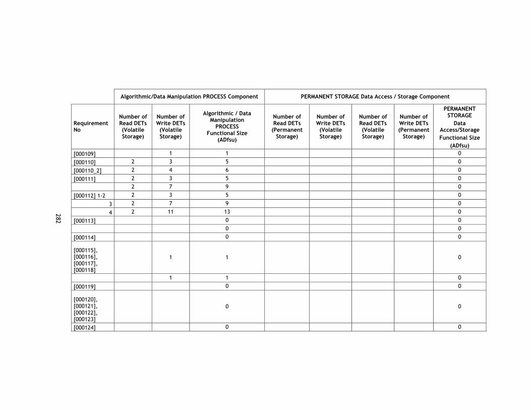
282

Algorithmic/Data Manipulation PROCESS Component PERMANENT STORAGE Data Access / Storage Component

Requirement No

Number of Read DETs (Volatile Storage)

Number of Write DETs (Volatile Storage)

Algorithmic / Data Manipulation

PROCESS Functional Size

(ADfsu)

Number of Read DETs

(Permanent Storage)

Number of Write DETs (Volatile Storage)

Number of Read DETs (Volatile Storage)

Number of Write DETs (Permanent

Storage)

PERMANENT STORAGE

Data Access/Storage Functional Size

(ADfsu) [000109] 1 1 0

[000110] 2 3 5 0

[000110_2] 2 4 6 0

[000111] 2 3 5 0

2 7 9 0

[000112] 1-2 2 3 5 0

3 2 7 9 0

4 2 11 13 0

[000113] 0 0

0 0

[000114] 0 0

[000115], [000116], [000117], [000118]

1 1 0

1 1 0

[000119] 0 0

[000120], [000121], [000122], [000123]

0 0

[000124] 0 0

283

Algorithmic/Data Manipulation PROCESS Component PERMANENT STORAGE Data Access / Storage Component

Requirement No

Number of Read DETs (Volatile Storage)

Number of Write DETs (Volatile Storage)

Algorithmic / Data Manipulation

PROCESS Functional Size

(ADfsu)

Number of Read DETs

(Permanent Storage)

Number of Write DETs (Volatile Storage)

Number of Read DETs (Volatile Storage)

Number of Write DETs (Permanent

Storage)

PERMANENT STORAGE

Data Access/Storage Functional Size

(ADfsu) [000125] 0 0

[000125_21] 0 0

[000125_22] 3 1 4 0

[000126] 3 80 83 0

3 78 81 0

[000127] 0 0

[000128] 0 0

[000129] 0 0

[000130] 0 0

[000131] 0 0

[000132] 0 0

3 78 81 0

[000133] 3 82 85 0

3 78 81 0

[000134] 0 0

[000135] 0 0

[000136] 0 0

[000137] 0 0

0 0

[000138] 0 0

[000139] 5 9 14 0

2 2 0

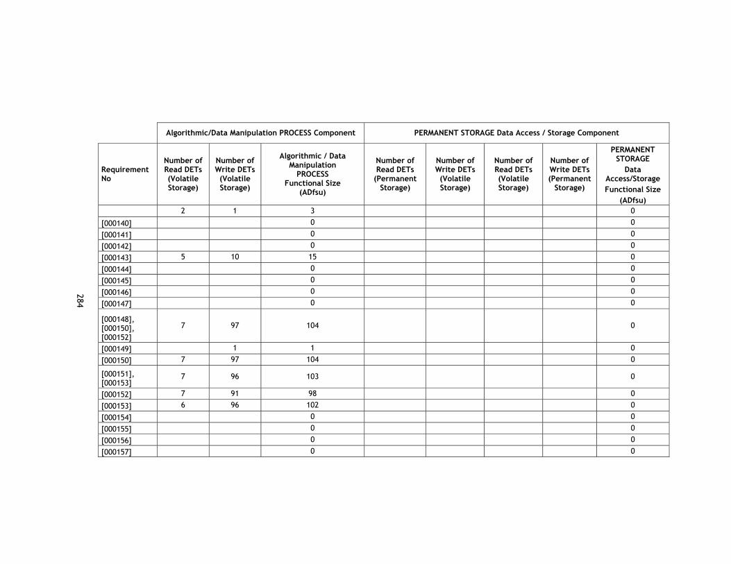
284

Algorithmic/Data Manipulation PROCESS Component PERMANENT STORAGE Data Access / Storage Component

Requirement No

Number of Read DETs (Volatile Storage)

Number of Write DETs (Volatile Storage)

Algorithmic / Data Manipulation

PROCESS Functional Size

(ADfsu)

Number of Read DETs

(Permanent Storage)

Number of Write DETs (Volatile Storage)

Number of Read DETs (Volatile Storage)

Number of Write DETs (Permanent

Storage)

PERMANENT STORAGE

Data Access/Storage Functional Size

(ADfsu) 2 1 3 0

[000140] 0 0

[000141] 0 0

[000142] 0 0

[000143] 5 10 15 0

[000144] 0 0

[000145] 0 0

[000146] 0 0

[000147] 0 0

[000148], [000150], [000152]

7 97 104 0

[000149] 1 1 0

[000150] 7 97 104 0

[000151], [000153]

7 96 103 0

[000152] 7 91 98 0

[000153] 6 96 102 0

[000154] 0 0

[000155] 0 0

[000156] 0 0

[000157] 0 0

285

Algorithmic/Data Manipulation PROCESS Component PERMANENT STORAGE Data Access / Storage Component

Requirement No

Number of Read DETs (Volatile Storage)

Number of Write DETs (Volatile Storage)

Algorithmic / Data Manipulation

PROCESS Functional Size

(ADfsu)

Number of Read DETs

(Permanent Storage)

Number of Write DETs (Volatile Storage)

Number of Read DETs (Volatile Storage)

Number of Write DETs (Permanent

Storage)

PERMANENT STORAGE

Data Access/Storage Functional Size

(ADfsu) 0 0

[000158] 0 0

Total 298 3,179 3,477 1 1 0 0 2

286

Case Study 3.3 – ARCHI-DIM FSM Measurement Catalogue

INTERFACE Component Control PROCESS Component

Requirement No

Number of Read DETs

(I/O Device)

Number of Write DETs (Volatile Storage)

Number of Read DETs (Volatile Storage)

Number of Write DETs (I/O Device)

INTERFACE Functional

Size (ADfsu)

Number of Read DETs (Volatile Storage)

Number of Write DETs (Volatile Storage)

Control PROCESS

Functional Size (ADfsu)

3.3.1.1.0, 3.3.1.1.5

1 1 35 35 72 0

3.3.1.1.1 31 31 36 36 134 0

3.3.1.1.2, 3.3.1.1.5

32 32 36 36 136 0

3.3.1.1.3 2 2 2 2 8 0

3.3.1.1.4, 3.3.1.1.5

2 2 36 36 76 0

3.3.1.1.5 0 0

3.3.1.1.6 0 0

3.3.1.2.2 6 6 10 10 32 0

3.3.1.3.1 10 10 10 10 40 0

3.3.1.3.2 8 8 10 10 36 0

3.3.1.3.3 2 2 11 11 26 0

3.3.1.4.1 12 12 13 13 50 0

3.3.1.4.2 13 13 13 13 52 0

3.3.1.4.3 2 2 14 14 32 0

3.3.1.5.1 0 0

2 2 3 3 10

Case Study 3.3 – ARCH

I-DIM

FSM M

easurement Catalogue

287

INTERFACE Component Control PROCESS Component

Requirement No

Number of Read DETs

(I/O Device)

Number of Write DETs (Volatile Storage)

Number of Read DETs (Volatile Storage)

Number of Write DETs (I/O Device)

INTERFACE Functional

Size (ADfsu)

Number of Read DETs (Volatile Storage)

Number of Write DETs (Volatile Storage)

Control PROCESS

Functional Size (ADfsu)

2 2 3 3 10

2 2 3 3 10

3.3.1.5.2 0 0

2 2 3 3 10

2 2 3 3 10

2 2 3 3 10

3.3.1.5.3 0 0

1 1 3 3 8

1 1 3 3 8

1 1 3 3 8

3.3.2.2.1 25 25 31 31 112 0

3.3.2.2.2 8 8 30 30 76 0

3.3.2.2.3 2 2 13 13 30 0

3.3.2.1.1 - 1 2 2 30 30 64 0

2 2 30 30 64

3.3.2.2.4.1 5 5 6 6 22 0

3.3.2.2.4.2 6 6 6 6 24 0

3.3.2.2.4.3 2 2 7 7 18 0

3.3.2.3.1 26 26 32 32 116 0

288

INTERFACE Component Control PROCESS Component

Requirement No

Number of Read DETs

(I/O Device)

Number of Write DETs (Volatile Storage)

Number of Read DETs (Volatile Storage)

Number of Write DETs (I/O Device)

INTERFACE Functional

Size (ADfsu)

Number of Read DETs (Volatile Storage)

Number of Write DETs (Volatile Storage)

Control PROCESS

Functional Size (ADfsu)

3.3.2.3.2 9 9 31 31 80 0

3.3.2.3.3 2 2 14 14 32 0

3.3.2.1.1-2 2 2 31 31 66 0

2 2 31 31 66

3.3.2.4.1 14 14 19 19 66 0

3.3.2.4.2 8 8 19 19 54 0

3.3.2.4.3 2 2 14 14 32 0

2 2 19 19 42 0

2 2 19 19 42

3.3.2.5.1 16 16 23 23 78 0

3.3.2.5.2 4 4 21 21 50 0

3.3.2.5.3 2 2 20 20 44 0

1 1 1 1 4

3.3.2.5.4 2 2 20 20 44

1 1 1 1 4

2 2 21 21 46 0

3.3.2.6.1, 3.3.1.2.1

19 19 25 25 88 0

3.3.2.6.2, 3.3.1.2.1

6 6 25 25 62 0

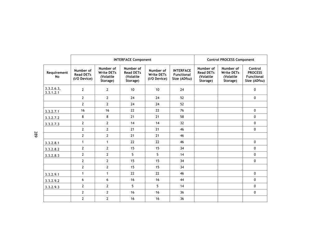
289

INTERFACE Component Control PROCESS Component

Requirement No

Number of Read DETs

(I/O Device)

Number of Write DETs (Volatile Storage)

Number of Read DETs (Volatile Storage)

Number of Write DETs (I/O Device)

INTERFACE Functional

Size (ADfsu)

Number of Read DETs (Volatile Storage)

Number of Write DETs (Volatile Storage)

Control PROCESS

Functional Size (ADfsu)

3.3.2.6.3, 3.3.1.2.1

2 2 10 10 24 0

2 2 24 24 52 0

2 2 24 24 52

3.3.2.7.1 16 16 22 22 76 0

3.3.2.7.2 8 8 21 21 58 0

3.3.2.7.3 2 2 14 14 32 0

2 2 21 21 46 0

2 2 21 21 46

3.3.2.8.1 1 1 22 22 46 0

3.3.2.8.2 2 2 15 15 34 0

3.3.2.8.3 2 2 5 5 14 0

2 2 15 15 34 0

2 2 15 15 34

3.3.2.9.1 1 1 22 22 46 0

3.3.2.9.2 6 6 16 16 44 0

3.3.2.9.3 2 2 5 5 14 0

2 2 16 16 36 0

2 2 16 16 36

290

INTERFACE Component Control PROCESS Component

Requirement No

Number of Read DETs

(I/O Device)

Number of Write DETs (Volatile Storage)

Number of Read DETs (Volatile Storage)

Number of Write DETs (I/O Device)

INTERFACE Functional

Size (ADfsu)

Number of Read DETs (Volatile Storage)

Number of Write DETs (Volatile Storage)

Control PROCESS

Functional Size (ADfsu)

3.3.2.10.1 11 11 18 18 58 0

3.3.2.10.2 3 3 17 17 40 0

2 2 17 17 38 0

2 2 17 17 38 0

2 2 15 15 34

3.3.2.11.1 7 7 10 10 34 0

2 2 13 13 30 0

2 2 13 13 30

3.3.2.12.1 1 1 6 6 14 0

2 2 11 11 26 0

2 2 11 11 26

3.3.2.12.2 1 1 6 6 14 0

2 2 11 11 26 0

2 2 11 11 26

3.3.2.12.3 0 0

3.3.2.12.4 1 1 3 3 8 0

2 2 8 8 20 0

2 2 8 8 20

3.3.3.1.1 13 13 18 18 62 0

291

INTERFACE Component Control PROCESS Component

Requirement No

Number of Read DETs

(I/O Device)

Number of Write DETs (Volatile Storage)

Number of Read DETs (Volatile Storage)

Number of Write DETs (I/O Device)

INTERFACE Functional

Size (ADfsu)

Number of Read DETs (Volatile Storage)

Number of Write DETs (Volatile Storage)

Control PROCESS

Functional Size (ADfsu)

3.3.3.1.2 14 14 18 18 64 0

3.3.3.1.3 3 3 14 14 34 0

2 2 18 18 40 0

2 2 18 18 40

3.3.3.2.1 14 14 19 19 66 0

3.3.3.2.2 15 15 19 19 68 0

3.3.3.2.3 3 3 15 15 36 0

2 2 19 19 42 0

2 2 19 19 42

3.3.3.3.1 12 12 17 17 58 0

3.3.3.3.2 6 6 17 17 46 0

3.3.3.3.3 3 3 13 13 32 0

2 2 17 17 38 0

2 2 17 17 38

3.3.3.4.1 10 10 15 15 50 0

3.3.3.4.2 4 4 15 15 38 0

3.3.3.4.3 3 3 11 11 28 0

2 2 15 15 34 0

2 2 15 15 34

292

INTERFACE Component Control PROCESS Component

Requirement No

Number of Read DETs

(I/O Device)

Number of Write DETs (Volatile Storage)

Number of Read DETs (Volatile Storage)

Number of Write DETs (I/O Device)

INTERFACE Functional

Size (ADfsu)

Number of Read DETs (Volatile Storage)

Number of Write DETs (Volatile Storage)

Control PROCESS

Functional Size (ADfsu)

3.3.3.5.1 9 9 14 14 46 0

3.3.3.5.2 5 5 14 14 38 0

3.3.3.5.3 3 3 10 10 26 0

2 2 14 14 32 0

2 2 14 14 32

3.3.4.1 1 1 3 3 8 0

3.3.4.2 1 1 3 3 8 0

1 1 3 3 8

3.3.4.3 1 1 3 3 8 0

3.3.4.4 1 1 3 3 8 0

1 1 3 3 8

3.3.5 0

1 1 2 1 1

1 1 2

Total 558,00 558,00 1,705.00 1,705.00 4,526.00 1,00 0,00 1,00

293

Algorithmic/Data Manipulation PROCESS Component PERMANENT STORAGE Data Access / Storage Component

Requirement No

Number of Read DETs (Volatile Storage)

Number of Write DETs (Volatile Storage)

Algorithmic / Data Manipulation

PROCESS Functional Size

(ADfsu)

Number of Read DETs

(Permanent Storage)

Number of Write DETs

(Volatile Storage)

Number of Read DETs (Volatile Storage)

Number of Write DETs (Permanent

Storage)

PERMANENT STORAGE

Data Access / Storage

Functional Size (ADfsu)

3.3.1.1.0, 3.3.1.1.5

0 34 34 68

3.3.1.1.1 0 34 34 33 33 134

3.3.1.1.2, 3.3.1.1.5

0 34 34 32 32 132

3.3.1.1.3 0 34 34 1 1 70

3.3.1.1.4, 3.3.1.1.5

0 34 34 1 1 70

3.3.1.1.5 0 0

3.3.1.1.6 0 31 31 31 31 124

3.3.1.2.2 0 9 9 6 6 30

3.3.1.3.1 0 9 9 10 10 38

3.3.1.3.2 0 9 9 7 7 32

3.3.1.3.3 0 9 9 1 1 20

3.3.1.4.1 0 12 12 13 13 50

3.3.1.4.2 0 12 12 12 12 48

3.3.1.4.3 0 12 12 1 1 26

3.3.1.5.1 0 0

0 2 2 2 2 8

294

Algorithmic/Data Manipulation PROCESS Component PERMANENT STORAGE Data Access / Storage Component

Requirement No

Number of Read DETs (Volatile Storage)

Number of Write DETs (Volatile Storage)

Algorithmic / Data Manipulation

PROCESS Functional Size

(ADfsu)

Number of Read DETs

(Permanent Storage)

Number of Write DETs

(Volatile Storage)

Number of Read DETs (Volatile Storage)

Number of Write DETs (Permanent

Storage)

PERMANENT STORAGE

Data Access / Storage

Functional Size (ADfsu)

0 2 2 2 2 8

0 2 2 2 2 8

3.3.1.5.2 0 0

0 2 2 1 1 6

0 2 2 1 1 6

0 2 2 1 1 6

3.3.1.5.3 0 0

0 2 2 1 1 6

0 2 2 1 1 6

0 2 2 1 1 6

3.3.2.2.1 8 3 11 39 39 30 30 138

3.3.2.2.2 0 31 31 8 8 78

3.3.2.2.3 2 2 4 14 14 5 5 38

3.3.2.1.1 - 1 0 31 31 62

0 31 31 1 1 64

3.3.2.2.4.1 0 7 7 5 5 24

3.3.2.2.4.2 0 7 7 5 5 24

3.3.2.2.4.3 0 5 5 1 1 12

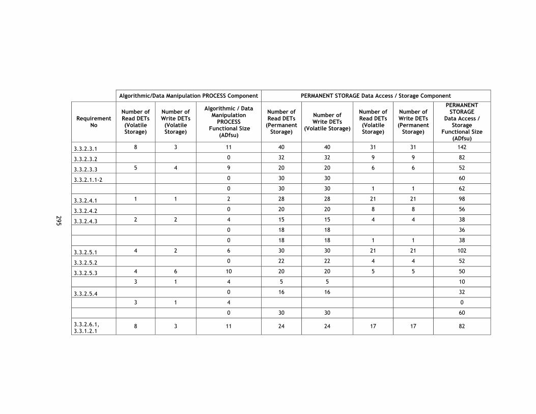
295

Algorithmic/Data Manipulation PROCESS Component PERMANENT STORAGE Data Access / Storage Component

Requirement No

Number of Read DETs (Volatile Storage)

Number of Write DETs (Volatile Storage)

Algorithmic / Data Manipulation

PROCESS Functional Size

(ADfsu)

Number of Read DETs

(Permanent Storage)

Number of Write DETs

(Volatile Storage)

Number of Read DETs (Volatile Storage)

Number of Write DETs (Permanent

Storage)

PERMANENT STORAGE

Data Access / Storage

Functional Size (ADfsu)

3.3.2.3.1 8 3 11 40 40 31 31 142

3.3.2.3.2 0 32 32 9 9 82

3.3.2.3.3 5 4 9 20 20 6 6 52

3.3.2.1.1-2 0 30 30 60

0 30 30 1 1 62

3.3.2.4.1 1 1 2 28 28 21 21 98

3.3.2.4.2 0 20 20 8 8 56

3.3.2.4.3 2 2 4 15 15 4 4 38

0 18 18 36

0 18 18 1 1 38

3.3.2.5.1 4 2 6 30 30 21 21 102

3.3.2.5.2 0 22 22 4 4 52

3.3.2.5.3 4 6 10 20 20 5 5 50

3 1 4 5 5 10

3.3.2.5.4 0 16 16 32

3 1 4 0

0 30 30 60

3.3.2.6.1, 3.3.1.2.1

8 3 11 24 24 17 17 82

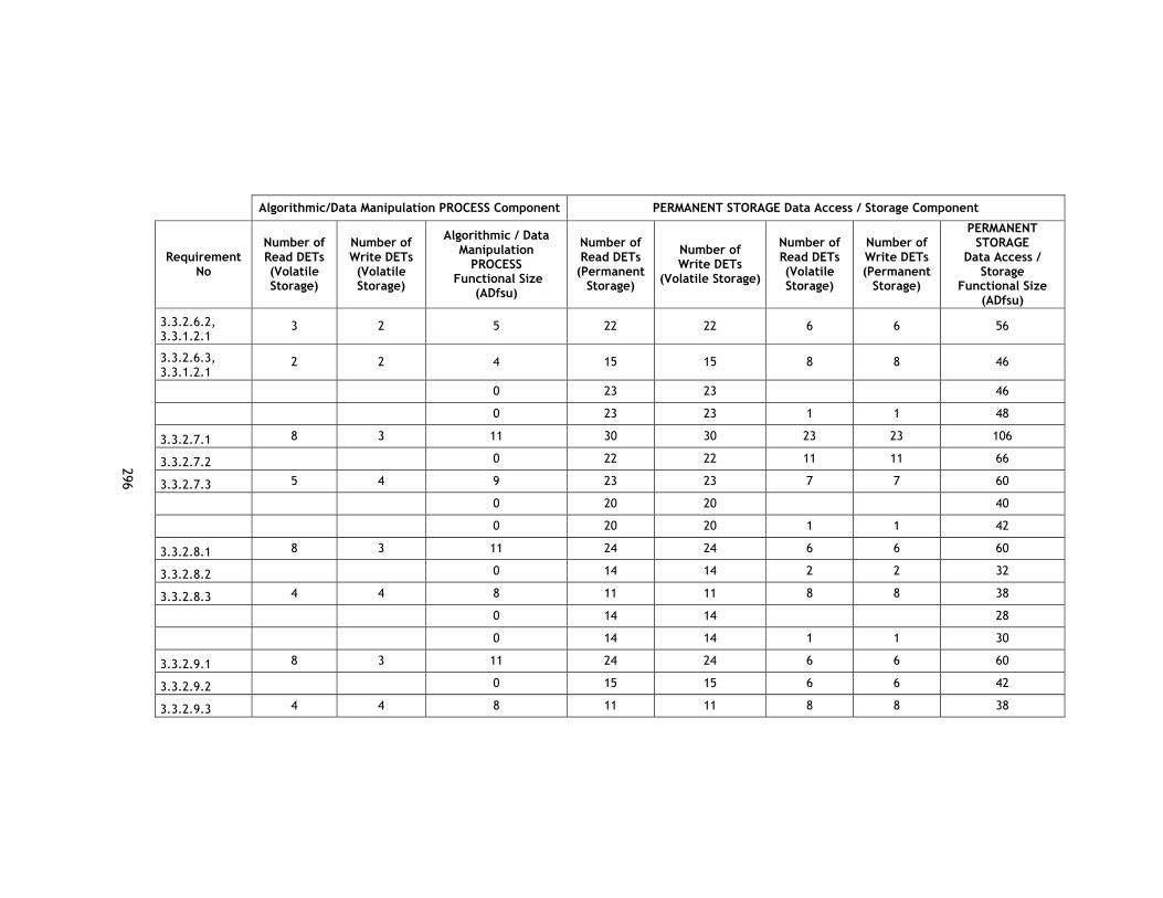
296

Algorithmic/Data Manipulation PROCESS Component PERMANENT STORAGE Data Access / Storage Component

Requirement No

Number of Read DETs (Volatile Storage)

Number of Write DETs (Volatile Storage)

Algorithmic / Data Manipulation

PROCESS Functional Size

(ADfsu)

Number of Read DETs

(Permanent Storage)

Number of Write DETs

(Volatile Storage)

Number of Read DETs (Volatile Storage)

Number of Write DETs (Permanent

Storage)

PERMANENT STORAGE

Data Access / Storage

Functional Size (ADfsu)

3.3.2.6.2, 3.3.1.2.1

3 2 5 22 22 6 6 56

3.3.2.6.3, 3.3.1.2.1

2 2 4 15 15 8 8 46

0 23 23 46

0 23 23 1 1 48

3.3.2.7.1 8 3 11 30 30 23 23 106

3.3.2.7.2 0 22 22 11 11 66

3.3.2.7.3 5 4 9 23 23 7 7 60

0 20 20 40

0 20 20 1 1 42

3.3.2.8.1 8 3 11 24 24 6 6 60

3.3.2.8.2 0 14 14 2 2 32

3.3.2.8.3 4 4 8 11 11 8 8 38

0 14 14 28

0 14 14 1 1 30

3.3.2.9.1 8 3 11 24 24 6 6 60

3.3.2.9.2 0 15 15 6 6 42

3.3.2.9.3 4 4 8 11 11 8 8 38

297

Algorithmic/Data Manipulation PROCESS Component PERMANENT STORAGE Data Access / Storage Component

Requirement No

Number of Read DETs (Volatile Storage)

Number of Write DETs (Volatile Storage)

Algorithmic / Data Manipulation

PROCESS Functional Size

(ADfsu)

Number of Read DETs

(Permanent Storage)

Number of Write DETs

(Volatile Storage)

Number of Read DETs (Volatile Storage)

Number of Write DETs (Permanent

Storage)

PERMANENT STORAGE

Data Access / Storage

Functional Size (ADfsu)

0 15 15 30

0 15 15 1 1 32

3.3.2.10.1 8 3 11 24 24 16 16 80

3.3.2.10.2 0 21 21 3 3 48

5 4 9 19 19 6 6 50

0 16 16 32

0 16 16 1 1 34

3.3.2.11.1 0 16 16 13 13 58

0 12 12 24

0 12 12 1 1 26

3.3.2.12.1 0 12 12 24

0 10 10 20

0 10 10 1 1 22

3.3.2.12.2 0 12 12 24

0 10 10 20

0 10 10 1 1 22

3.3.2.12.3 0 0

3.3.2.12.4 0 12 12 24

298

Algorithmic/Data Manipulation PROCESS Component PERMANENT STORAGE Data Access / Storage Component

Requirement No

Number of Read DETs (Volatile Storage)

Number of Write DETs (Volatile Storage)

Algorithmic / Data Manipulation

PROCESS Functional Size

(ADfsu)

Number of Read DETs

(Permanent Storage)

Number of Write DETs

(Volatile Storage)

Number of Read DETs (Volatile Storage)

Number of Write DETs (Permanent

Storage)

PERMANENT STORAGE

Data Access / Storage

Functional Size (ADfsu)

0 7 7 14

0 7 7 1 1 16

3.3.3.1.1 1 1 2 19 19 17 17 72

3.3.3.1.2 1 1 2 17 17 13 13 60

3.3.3.1.3 2 2 4 17 17 3 3 40

0 17 17 34

0 17 17 1 1 36

3.3.3.2.1 1 1 2 20 20 18 18 76

3.3.3.2.2 1 1 2 18 18 14 14 64

3.3.3.2.3 2 2 4 16 16 3 3 38

0 17 17 34

0 17 17 1 1 36

3.3.3.3.1 3 2 5 24 24 16 16 80

3.3.3.3.2 3 2 5 16 16 12 12 56

3.3.3.3.3 2 2 4 15 15 4 4 38

0 16 16 32

0 16 16 1 1 34

3.3.3.4.1 1 1 2 20 20 14 14 68

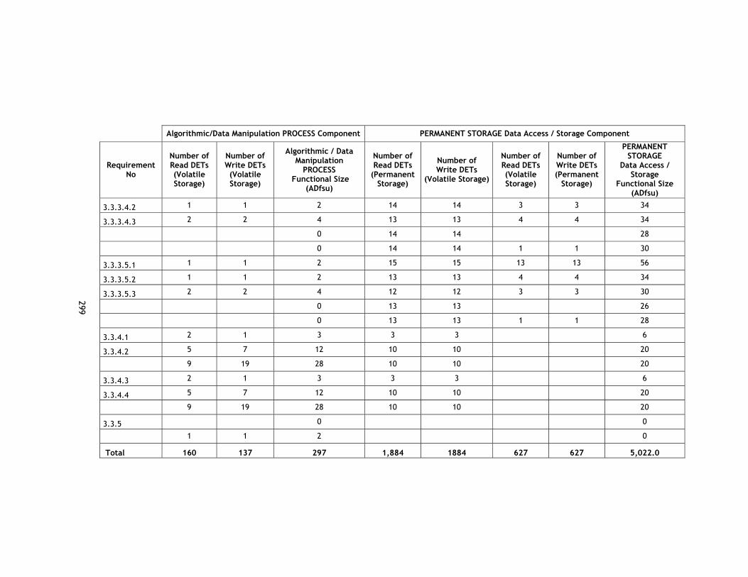
299

Algorithmic/Data Manipulation PROCESS Component PERMANENT STORAGE Data Access / Storage Component

Requirement No

Number of Read DETs (Volatile Storage)

Number of Write DETs (Volatile Storage)

Algorithmic / Data Manipulation

PROCESS Functional Size

(ADfsu)

Number of Read DETs

(Permanent Storage)

Number of Write DETs

(Volatile Storage)

Number of Read DETs (Volatile Storage)

Number of Write DETs (Permanent

Storage)

PERMANENT STORAGE

Data Access / Storage

Functional Size (ADfsu)

3.3.3.4.2 1 1 2 14 14 3 3 34

3.3.3.4.3 2 2 4 13 13 4 4 34

0 14 14 28

0 14 14 1 1 30

3.3.3.5.1 1 1 2 15 15 13 13 56

3.3.3.5.2 1 1 2 13 13 4 4 34

3.3.3.5.3 2 2 4 12 12 3 3 30

0 13 13 26

0 13 13 1 1 28

3.3.4.1 2 1 3 3 3 6

3.3.4.2 5 7 12 10 10 20

9 19 28 10 10 20

3.3.4.3 2 1 3 3 3 6

3.3.4.4 5 7 12 10 10 20

9 19 28 10 10 20

3.3.5 0 0

1 1 2 0

Total 160 137 297 1,884 1884 627 627 5,022.0

300

VITA Çiğdem Gencel was born in Ankara on April 17, 1973. She received the BSc and MSc degree

in environmental engineering from Middle East Technical University (METU), in 1995 and in

1998, respectively. She worked as a project assistant for MEDCOAST located in METU

between 1995 and 1998. She has been working as a teaching assistant in Informatics

Institute, METU since 1998.

Between 2001 and 2005, she worked on various projects, which involve a project on online

course content preparation for a course on information technologies and applications, a

research funds project on 3-D brain image processing, two projects on preparation of

Request for Proposals for C4ISR systems for Turkish Land Forces Command and a project on

the development of a conceptual modeling development tool for modeling and simulation

of C4ISR Systems for Undersecretariat for Defense Industries.

Her research interests involve software metrics, software size estimation and

measurement, software requirements elicitation, image processing and 3-D image

registration.