Int. J. Electron. Commun. (AEU) 58 (2004): 37–40http://www.elsevier-deutschland.de/aeue

Letter

An Approach to the Control ofPeriodically Cyclic Processes

Robert Bauer and Nicolaos Dourdoumas

Dedicated to Professor Klaus Meerkötter on the occasionof his 60th birthday

Abstract: Numerous solutions for the problem of controlling peri-odically cyclic processes (i.e. systems subject to periodic referencesignals) already exist. However, most of them are quite sophis-ticated, hence unfavourable in practice. The following method isvery simple, easily realisable, needs little prior knowledge of thesystem, works even with non-minimum-phase systems or systemswith large dead time and has proved to function by some industrialapplications.

Keywords: Periodically cyclic process, Nonparametric identifica-tion

1. Introduction

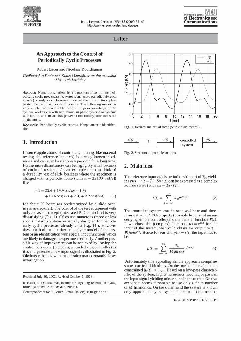
In some applications of control engineering, like materialtesting, the reference input r(t) is already known in ad-vance and can even be stationary periodic for a long time.Furthermore disturbances can be negligibly small becauseof enclosed testbeds. As an example one can think ofa durability test of slide bearings where the specimen ischarged with a periodic force (with ω = 2π100 [rad/s])like

r(t) = 23.6 +19.9 cos(ωt −1.9)

+10.6 cos(2ωt +2.9)+2.2 cos(3ωt) (1)

for about 50 hours (as predetermined by a slide bear-ing manufacturer). The control of the test equipment withonly a classic concept (integrated PID-controller) is verydissatisfying (Fig. 1). Of course numerous (more or lesssophisticated) solutions especially designed for periodi-cally cyclic processes already exist (e.g. [4]). Howeverthese methods need either an analytic model of the sys-tem or an identification with special input functions whichare likely to damage the specimen seriously. Another pos-sible way of improvement can be achieved by leaving thecontrolled system (including an underlying controller) asit is and generate a new input signal as illustrated in Fig. 2.Obviously the box with the question mark demands closerinvestigation.

Received July 30, 2003. Revised October 6, 2003.

R. Bauer, N. Dourdoumas, Institut für Regelungstechnik, TU Graz,Inffeldgasse 16c, A-8010 Graz, Austria.

Correspondence to: R. Bauer. E-mail: bauer@irt.tu-graz.ac.at

� � � � � � � � � � � � � � � � ��

� �

� �

� �

� �

� �

� �

� � �

����������

�

� � �� � �

� � � � � � � � � � � � � � � � ��

� �

� �

� �

� �

� �

� �

� � �

����������

�

� � �� � �

Fig. 1. Desired and actual force (with classic control).

�� � � � � � � � � � � � � � � � �

� � � � �

� � � �

Fig. 2. Structure of possible solution.

2. Main idea

The reference input r(t) is periodic with period T0, yield-ing r(t) = r(t + T0). So r(t) can be expressed as a complexFourier series (with ω0 = 2π/T0):

r(t) =∞∑

m=−∞Rme jmω0t (2)

The controlled system can be seen as linear and time-invariant with BIBO-property (possibly because of an un-derlying simple controller) and the transfer function P(s).If we chose the (complex) function u(t) = e jωt for theinput of the system, we would obtain the output y(t) =P( jω)e jωt. Hence for our aim y(t) = r(t) the input has tobe:

u(t) =∞∑

m=−∞

Rm

P( jmω0)e jmω0t (3)

Unfortunately this appealing simple approach comprisessome practical difficulties. On the one hand a real input isconstrained |u(t)| ≤ umax. Based on a low-pass character-istic of the system, higher harmonics need major parts inthe input signal yielding minor parts in the output. On thataccount it seems reasonable to use only a finite numberof M harmonics. On the other hand the system is knownonly approximately, so system identification is needed.

1434-8411/04/58/01-037 $ 30.00/0

38 R. Bauer, N. Dourdoumas: An Approach to the Control of Periodically Cyclic Processes

The system also may vary during operation, therefore theidentification has to be repetitive.

As a first step the necessary input signal

u(t) =M∑

m=−M

Rm

Pme jmω0t (4)

is calculated – based on the values Pm = P( jmω0) of anestimated transfer function P(s) – and sent to the realsystem. After decay of transients the estimated valuesPm of the frequency response can be improved using the(measured) output signal y(t). With these improved es-timates Pm a new necessary input function is obtained.The repetition of the above operation sequence will re-sult in an output y(t) becoming more and more simi-lar to the desired input r(t). For lack of better initialtransfer function estimations, P(s) = 1 would be a goodchoice.

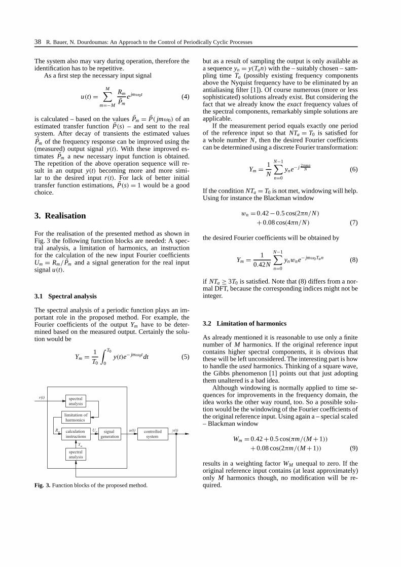
3. Realisation

For the realisation of the presented method as shown inFig. 3 the following function blocks are needed: A spec-tral analysis, a limitation of harmonics, an instructionfor the calculation of the new input Fourier coefficientsUm = Rm/Pm and a signal generation for the real inputsignal u(t).

3.1 Spectral analysis

The spectral analysis of a periodic function plays an im-portant role in the proposed method. For example, theFourier coefficients of the output Ym have to be deter-mined based on the measured output. Certainly the solu-tion would be

Ym = 1

T0

∫ T0

0y(t)e− jmω0tdt (5)

� � � � � � � � �

� � � � �

� � � � � � � � � � �

� � � � � � � � � � � �

� � � � � � � �

� � � � � � � �

� � � � � �

� � � � � � � � � �

� � � � � � � �

� � � � � � � �

� � � � � � � � � � �

� � � � � � � �

� �

�

� � � � � � � � �

� � � �

Fig. 3. Function blocks of the proposed method.

but as a result of sampling the output is only available asa sequence yn = y(Tan) with the – suitably chosen – sam-pling time Ta (possibly existing frequency componentsabove the Nyquist frequency have to be eliminated by anantialiasing filter [1]). Of course numerous (more or lesssophisticated) solutions already exist. But considering thefact that we already know the exact frequency values ofthe spectral components, remarkably simple solutions areapplicable.

If the measurement period equals exactly one periodof the reference input so that NTa = T0 is satisfied fora whole number N, then the desired Fourier coefficientscan be determined using a discrete Fourier transformation:

Ym = 1

N

N−1∑n=0

yne− j 2πmnN (6)

If the condition NTa = T0 is not met, windowing will help.Using for instance the Blackman window

wn = 0.42 −0.5 cos(2πn/N)

+0.08 cos(4πn/N) (7)

the desired Fourier coefficients will be obtained by

Ym = 1

0.42N

N−1∑n=0

ynwne− jmω0Tan (8)

if NTa ≥ 3T0 is satisfied. Note that (8) differs from a nor-mal DFT, because the corresponding indices might not beinteger.

3.2 Limitation of harmonics

As already mentioned it is reasonable to use only a finitenumber of M harmonics. If the original reference inputcontains higher spectral components, it is obvious thatthese will be left unconsidered. The interesting part is howto handle the used harmonics. Thinking of a square wave,the Gibbs phenomenon [1] points out that just adoptingthem unaltered is a bad idea.

Although windowing is normally applied to time se-quences for improvements in the frequency domain, theidea works the other way round, too. So a possible solu-tion would be the windowing of the Fourier coefficients ofthe original reference input. Using again a – special scaled– Blackman window

Wm = 0.42 +0.5 cos(πm/(M +1))

+0.08 cos(2πm/(M +1)) (9)

results in a weighting factor WM unequal to zero. If theoriginal reference input contains (at least approximately)only M harmonics though, no modification will be re-quired.

R. Bauer, N. Dourdoumas: An Approach to the Control of Periodically Cyclic Processes 39

3.3 Calculation instructions

Now we need a formula for improving the estimatedvalues Pm of the frequency response. Additional indicesindicate the iteration chronology. Based on the currentFourier coefficients of the input Um,i and the output Ym,i ,the next estimate

Pm,i+1 = Ym,i

Um,i(10)

seems to be a good choice, at least presuming ideal condi-tions. In reality the output coefficients are noisy, so addi-tional smoothing is required. A simple way of smoothingis obtained by a first-order discrete low-pass filter with thetransfer function

H(z) = qz

z − (1 −q)(11)

(with 0 < q ≤ 1), now applied as shown in Fig. 4. Thiswould result in a linear approach in the complex plane(as indicated in Fig. 5) with the disadvantage of temporarysmall absolute values exciting large input signals. A pos-sible solution is the application of the filter separately tomagnitude and phase yielding:

Pm,i+1 = [(1 −q)|Pm,i|+q|Ym,i/Um,i|

]· e j[(1−q) arg(Pm,i )+q arg(Ym,i/Um,i )] (12)

This results in the upper, clockwise and (above all) longerpath inside the grey annulus (again Fig. 5). The reason for

� � � � � � � � �

� � � � � �

�

Fig. 4. Low-pass filter applied to estimation.

� � � � � � � � � � � � � � � � � � � � � � � � � � � �� �

� � � �

� �

� � � �

�

� � �

�

� � �

�

� � � � � � � � � � � � � � � � � � � � � � � � � � � �� �

� � � �

� �

� � � �

�

� � �

�

� � �

�

� � � � � � �

� � � � � � � �

� � � �

�

� � � �

�

�

�

Fig. 5. Estimation paths in the complex plane of frequency re-sponse values.

� � � � � � � � � � � � � � � � ��

� �

� �

� �

� �

� �

� �

� � �

����������

�

� � �� � �

� � � � � � � � � � � � � � � � ��

� �

� �

� �

� �

� �

� �

� � �

����������

�

� � �� � �

Fig. 6. Desired and actual force (with the proposed method).

the longer path is the periodicity of the phase, hence

Pm,i+1 = [(1 −q)|Pm,i|+q|Ym,i/Um,i |

](13)

· e j[arg(Pm,i )+qwrap(arg(Ym,i/Um,i )−arg(Pm,i ))]

with wrap(ϕ) = arg(e jϕ) provides the correct path withinthe grey annulus. Finally

Um,i+1 = Rm

Pm,i+1(14)

yields the next input coefficients.

3.4 Signal generation

After determination of the input coefficients Um , the inputfunction

u(t) = U0 +M∑

m=1

2|Um| cos(mω0t + arg(Um)) (15)

has to be sent to the real system. Using a zero-orderhold as usual, a piecewise constant function is gener-ated containing unintended frequency components whichhave to be eliminated by a reconstruction filter [1]. How-ever an ideal reconstruction filter is not realisable, sothe generated signal u(t) differs slightly from the de-termined coefficients Um . But astonishingly this doesn’tmatter at all since the coefficients are altered just insuch a way that the output will have a desired be-haviour.

By choosing the sampling time Ta small enough, thelow-pass filter characteristic of the system itself corres-ponds to a reconstruction filter and additional hardwarecan be omitted.

40 R. Bauer, N. Dourdoumas: An Approach to the Control of Periodically Cyclic Processes

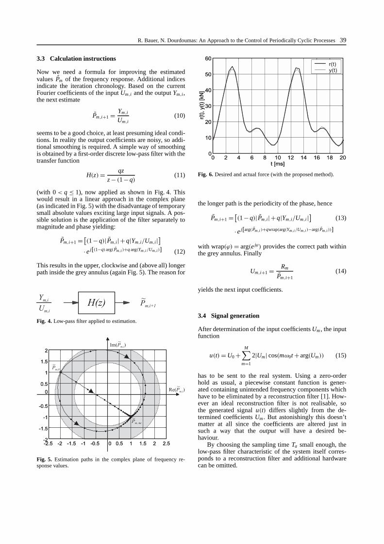
4. Results

The slide bearing testbed is controlled in a satisfactorymanner with the proposed method (as shown in Fig. 6)and already works successfully for a long period oftime.

Summarising, the proposed method is generally ap-plicable for slowly time-varying processes with periodicreferences and negligible disturbances. Without any an-alytic modelling and only little previous knowledge ityields an output signal almost identical to the refer-ence signal. Since it is not based on a classic inver-sion of a system, the concept works as well with non-

minimum-phase systems and systems with large deadtime.

References

[1] Oppenheim, A.V.; Schafer, R.W.: Discrete-time signal process-ing, Prentice Hall, New Jersey, 1999.

[2] Leonhard, W.: Digitale Signalverarbeitung in der Meß- undRegelungstechnik, Teubner, Stuttgart, 1989.

[3] Schüßler, H.W.: Digitale Signalverarbeitung 1, Springer Ver-lag, Berlin, 1994.

[4] Wagner, B.: Iterativ lernende Regelungen für periodisch zyk-lische Prozesse. Automatisierungstechnik 47 (1999), 89–93.