An application of the logistic curve to the modelingof CO2 emission reduction

Kazushi Hatase

Graduate School of Economics, Kobe University

2007/10/7 SEEPS Annual Meeting, Shiga University 2

The model and simulations of this study

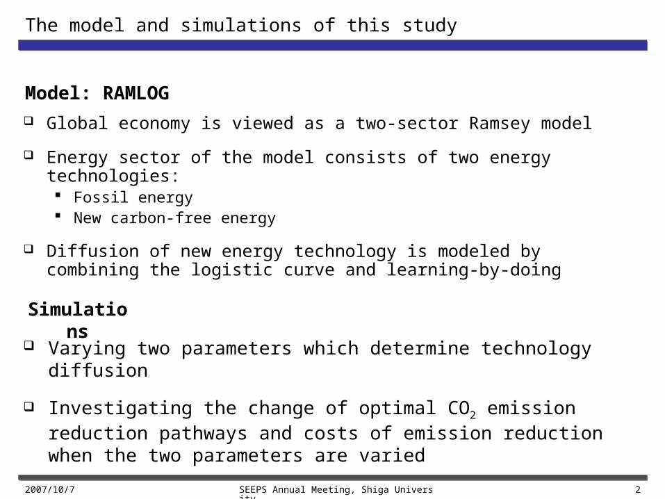
Model: RAMLOG

Global economy is viewed as a two-sector Ramsey model

Energy sector of the model consists of two energy technologies: Fossil energy New carbon-free energy

Diffusion of new energy technology is modeled by combining the logistic curve and learning-by-doing

Simulations

Varying two parameters which determine technology diffusion

Investigating the change of optimal CO2 emission reduction pathways and costs of emission reduction when the two parameters are varied

2007/10/7 SEEPS Annual Meeting, Shiga University 3

Preceding studies and significance of this study

Energy-economy models with substitutable two (fossil & new) energies

Goulder & Schneider (1999)

DEMETER

(2002)

ENTICE-BR

(2006)This study

Technological change

R&DLearning-by-

doingR&D

Learning-by- doing

Elasticity between two energies (σ)

σ=0.9 σ=2, 3, 4 σ=1.6, 2.2, 8.7Determined by logistic curve

Significance of this study

Diffusion of low CO2-emitting energy is crucial in climate change mitigation. This study proposes a model of long-term technology diffusion.

Logistic curve provides more realistic projection of future technology diffusion than the use of fixed elasticity between fossil and new energies.

Influence of technology-related parameters on CO2 emission reduction is examined.

2007/10/7 SEEPS Annual Meeting, Shiga University 4

Model of global economy (the Ramsey model)

1. Intertemporal utility maximization

2. Production function

　 　

3. Capital accumulation

4. Income accounts identity

　 　

0

max 1 logT

t

t t t tt

V L C L

1 11

1t t t t t tY K L E

1 1t t tK K I

, t t t t t t tY C I EC EC p E

t 0: labor inputs : pure time preference; exp t tL d t

: energy inputs , : parameterst t tE

: energy production coststEC

2007/10/7 SEEPS Annual Meeting, Shiga University 5

Logistic curve

Energy inputs consist of two energy technologies

Share of the new energy grows following the logistic curve

Modifying the equation above into the inequality form:

Finite difference form is used in the computer program:

1tt t

dSaS S

dt

1tt t

dSaS S

dt

1 1t t t tS S aS S t

1 1 1

1 1t t t t t t t t tY K L S E S E

1 : fossil energy inputs : new energy inputs : share of new energyt t t t tS E S E S

: coefficienta

2007/10/7 SEEPS Annual Meeting, Shiga University 6

Logistic curve (continued)

Coefficient determines the speed of diffusion in

It determines the “potential” speed of diffusion in

In the inequality form, diffusion trajectory can take any paths under the logistic curve

0%

20%

40%

60%

80%

100%

0 5 10 15 20 25 30 35 40

Shar

e of

new

ene

rgy

a 1t t tdS dt aS S

1t t tdS dt aS S

curve with small a

curve with large a

2007/10/7 SEEPS Annual Meeting, Shiga University 7

Learning-by-doing

Price of fossil energy is constant

　 　

Price of new energy declines as experience increases

Data of experience index （ source: McDonald & Schrattenholzer, 2001 ）

Technology Period Value of b

Nuclear (OECD) 1975 – 1993 0.09

GTCC （ OECD ） 1984 – 1994 0.60

Wind (OECD) 1981 – 1995 0.27

Photovoltaics (OECD) 1968 – 1998 0.32

Ethanol (Brazil) 1979 – 1995 0.32

,F t Fp p

, ,00

b

tN t N

Wp p

W

Fp

Np

: cumulative experience : experience indextW b

2007/10/7 SEEPS Annual Meeting, Shiga University 8

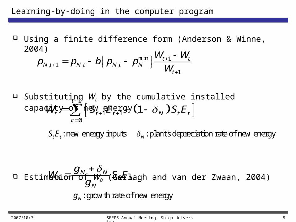
Learning-by-doing in the computer program

Using a finite difference form (Anderson & Winne, 2004)

Substituting Wt by the cumulative installed capacity of new energy

　

Estimation of W0 (Gerlagh and van der Zwaan, 2004)

0 0 0N N

N

gW S E

g

min 1, 1 , ,

1

t tN t N t N t N

t

W Wp p b p p

W

1

1 10

1t

t t t N t tW S E S E

: new energy inputs : plant's depreciation rate of new energyt t NS E

: growth rate of new energyNg

2007/10/7 SEEPS Annual Meeting, Shiga University 9

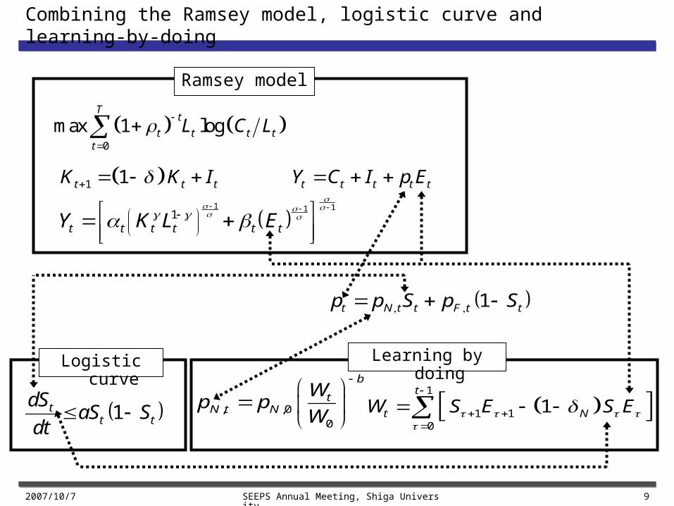
Combining the Ramsey model, logistic curve and learning-by-doing

0

max 1 logT

t

t t t tt

L C L

Ramsey model

1 11

1t t t t t tY K L E

1t N t t F t tp p S p S

1tt t

dSaS S

dt , ,0

0

b

tN t N

Wp p

W

1 1 t t t t t t t tK K I Y C I p E

1

1 10

1t

t NW S E S E

Logistic curve Learning by doing

2007/10/7 SEEPS Annual Meeting, Shiga University 10

Climate change model

Adopt a simple CO2 accumulation model (Grubb et al., 1995)

Anthropogenic CO2 emission

Natural CO2 emission (adopting DEMETER’s parameterization)

1Anth Nat

t t t t tM M Emis Emis M

maxtM M

max2: CO accumulation stabilization target (500ppm) : removal rateM M : 　

1Antht F t tEmis S E : emission intensity of fossil energyF

Nat NattEmis Emis : 1.33 /NatEmis GtC yr

2007/10/7 SEEPS Annual Meeting, Shiga University 11

Simulation scenarios

Simulation is lead to a time path of emissions that satisfies the stabilization target of 500ppm (cost-effectiveness simulation)

Investigating how Potential speed of technological change (coefficient a) Leaning rate (experience index:b)

affect CO2 emission reduction pathways and the costs of reduction

Run : coefficient of logistic curve b: experience index

(a) STC + LL 0.05 0.1

(b) STC + HL 0.05 0.5

(c) FTC + LL 0.15 0.1

(d) FTC + HL 0.15 0.5

STC: Slow Technological Change FTC: Fast Technological Change

LL: Low Learning HL: High Learning

Model runs and parameter settings

a

2007/10/7 SEEPS Annual Meeting, Shiga University 12

Common parameters (mainly adopted from DEMETER model)

Parameter Description Value

K(0) Capital in 2000 76.746 $trillion

Y(0) Gross output (GWP) in 2000 29.068 $trillion

E(0) Total energy input in 2000 6.628 GtC

δ Depreciation rate on capital 7%/year

γ Capital’s value share 0.31

σ Elasticity between K-L and E 0.40

S(0) Share of new energy in 2000 4.2%

pF Price of fossil energy 276.29 $/tC

pN (0) Price of new energy in 2000 1000 $/tC

pNmin

Lowest possible cost of new energy 250 $/tC

σN Plant’s depreciation rate of new energy 7%/year

gN Growth rate of new energy inputs 4.8%/year

M(0) Carbon accumulation in the atmosphere in 2000 786 GtC

μ Removal rate of CO2 from the atmosphere 0.6%/year

θF Emission intensity of fossil energy 1.0

EmisNat Natural CO2 emission in 2000 1.33 GtC/year

2007/10/7 SEEPS Annual Meeting, Shiga University 13

Calibration of the production function (based on MERGE model’s method)

1. Setting up the reference values of Y(t), K(t), E(t)

2. Differentiating and rearranging the production function to obtain α and β

00REF

A t L tY t Y

L

00REF

A t L tK t K

L

1

0 10

t

REF

A t L tE t E EEI

L

1

1

0 REF

REF

p Y tt

E t

1 1

11

REF REF

REF

Y t t E tt

K t L t

: labor productivity : energy efficiency improvementA t EEI t

2007/10/7 SEEPS Annual Meeting, Shiga University 14

Optimal CO2 emission pathways

Four emission pathways are not very different Learning-by-doing has almost no effect in STC (slow technological

change)

5

10

15

20

2000

2010

2020

2030

2040

2050

2060

2070

2080

2090

2100

2110

2120

2130

2140

2150

Em

issi

on (G

tC) BaU case

STC + LL

STC + HL

FTC + LL

FTC + HL

2007/10/7 SEEPS Annual Meeting, Shiga University 15

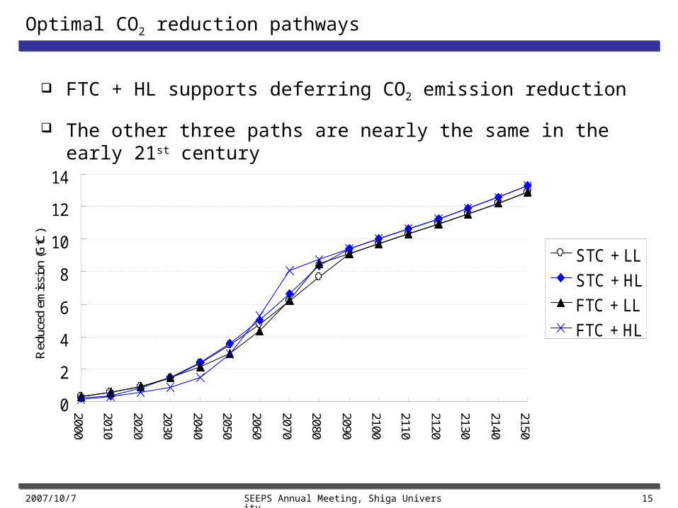
Optimal CO2 reduction pathways

0

2

4

6

8

10

12

14

2000

2010

2020

2030

2040

2050

2060

2070

2080

2090

2100

2110

2120

2130

2140

2150

Red

uced

em

issi

on (G

tC)

STC + LL

STC + HL

FTC + LL

FTC + HL

FTC + HL supports deferring CO2 emission reduction

The other three paths are nearly the same in the early 21st century

2007/10/7 SEEPS Annual Meeting, Shiga University 16

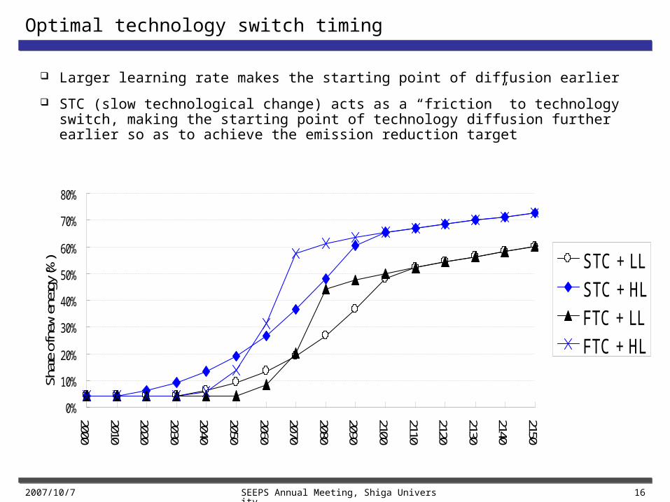
Optimal technology switch timing

Larger learning rate makes the starting point of diffusion earlier

STC (slow technological change) acts as a “friction” to technology switch, making the starting point of technology diffusion further earlier so as to achieve the emission reduction target

0%

10%

20%

30%

40%

50%

60%

70%

80%

2000

2010

2020

2030

2040

2050

2060

2070

2080

2090

2100

2110

2120

2130

2140

2150

Shar

e of

new

ene

rgy (

%) STC + LL

STC + HL

FTC + LL

FTC + HL

2007/10/7 SEEPS Annual Meeting, Shiga University 17

Emission reduction by reducing energy input and by new energy

0

2

4

6

8

10

12

14

2000

2010

2020

2030

2040

2050

2060

2070

2080

2090

2100

2110

2120

2130

2140

2150

Red

uced

em

issi

on (

GtC

)

0

2

4

6

8

10

12

14

2000

2010

2020

2030

2040

2050

2060

2070

2080

2090

2100

2110

2120

2130

2140

2150

Red

uced

em

issi

on (

GtC

)

0

2

4

6

8

10

12

14

2000

2010

2020

2030

2040

2050

2060

2070

2080

2090

2100

2110

2120

2130

2140

2150

Red

uced

em

issi

on (G

tC)

by reducing energy input

by new energy

0

2

4

6

8

10

12

14

2000

2010

2020

2030

2040

2050

2060

2070

2080

2090

2100

2110

2120

2130

2140

2150

Red

uced

em

issi

on (

GtC

)

(a) STC + LL

(c) FTC + LL

(b) STC + HL

(d) FTC + HL

2007/10/7 SEEPS Annual Meeting, Shiga University 18

Loss of GWP through CO2 emission reduction

0%

2%

4%

6%

8%

20

00

20

10

20

20

20

30

20

40

20

50

20

60

20

70

20

80

20

90

21

00

21

10

21

20

21

30

21

40

21

50

GW

P L

oss STC + LL

STC + HL

FTC + LL

FTC + HL

GWP loss largely depends on the learning rate

Pathways with the same learning rate are close or the same in the early and late period

2007/10/7 SEEPS Annual Meeting, Shiga University 19

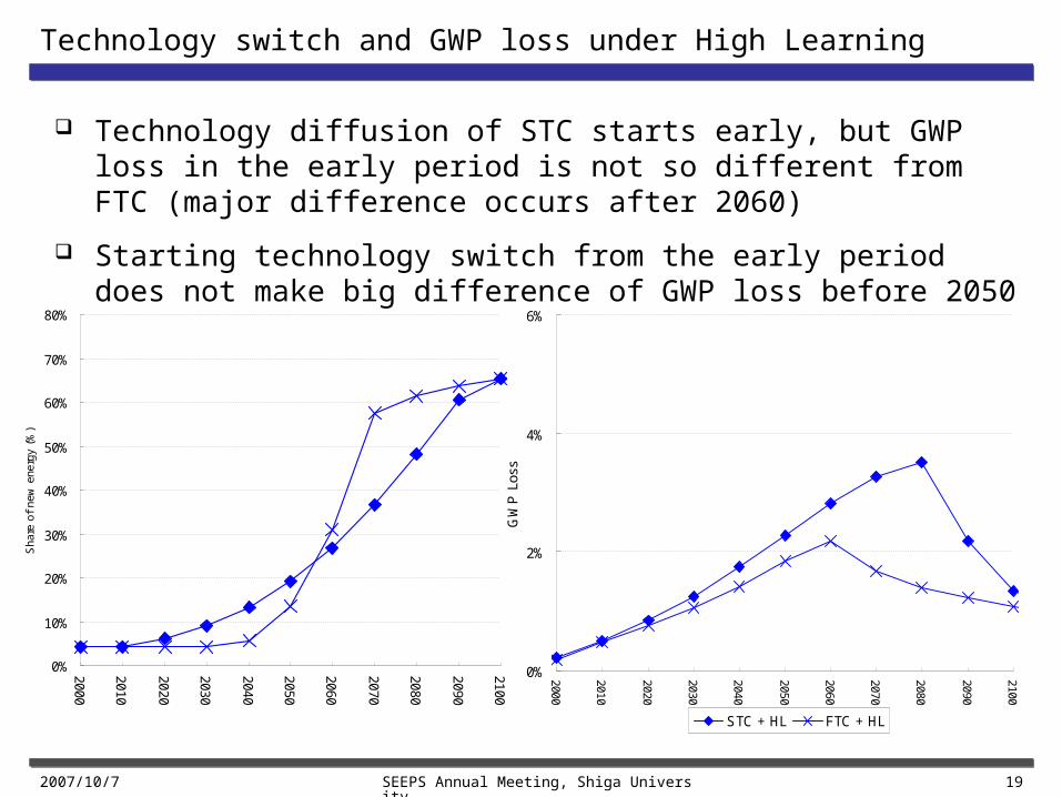
Technology switch and GWP loss under High Learning

0%

10%

20%

30%

40%

50%

60%

70%

80%

2000

2010

2020

2030

2040

2050

2060

2070

2080

2090

2100

Sha

re o

f ne

w e

nerg

y (%

)

0%

2%

4%

6%

2000

2010

2020

2030

2040

2050

2060

2070

2080

2090

2100

GW

P L

oss

STC + HL FTC + HL

Technology diffusion of STC starts early, but GWP loss in the early period is not so different from FTC (major difference occurs after 2060)

Starting technology switch from the early period does not make big difference of GWP loss before 2050

2007/10/7 SEEPS Annual Meeting, Shiga University 20

Carbon tax levels

0

20

40

60

80

100

120

2000

2010

2020

2030

2040

2050

2060

2070

2080

2090

2100

2110

2120

2130

2140

2150

Car

bon

tax

($/tC

)

STC + LL

STC + HL

FTC + LL

FTC + HL

Patterns are similar to those of GWP loss

Pathways of the same learning rate are the same in the early and late period

2007/10/7 SEEPS Annual Meeting, Shiga University 21

Conclusions

1. Progress of new carbon free technology justifies deferring CO2 emission reduction only in the case of FTC (fast technological change) + HL (high learning).

2. Optimal CO2 reduction paths are relatively similar between the 4 model runs, while the optimal technology diffusion paths diverge.

3. Larger learning rate makes the starting point of technology diffusion earlier.

4. Slow technological change acts as a “friction” to technology switch,

making the starting point of technology diffusion further earlier so as to achieve the emission reduction target.

5. GWP loss largely depends on the learning rate. Pathways of GWP loss with the same learning rate are close or the same in the early and late period.